When your Worker slows down or starts throwing errors, finding the root cause shouldn’t require hours of log analysis and trial-and-error debugging. You should have clear visibility into what’s happening at every step of your application’s request flow. This is feedback we’ve heard loud and clear from developers using Workers, and today we’re excited to announce an Open Beta for tracing on Cloudflare Workers! You can now:
Get automatic instrumentation for applications on the Workers platform: No manual setup, complex instrumentation, or code changes. It works out of the box.
Explore and investigate traces in the Cloudflare dashboard: Your traces are processed and available in the Workers Observability dashboard alongside your existing logs.
Export logs and traces to OpenTelemetry-compatible providers: Send OpenTelemetry traces (and correlated logs) to your observability provider of choice.
In 2024, we set out to build the best first-party observability of any cloud platform. We launched a new metrics dashboard to give better insights into how your Worker is performing, Workers Logs to automatically ingest and store logs for your Workers, a query builder to explore your data across any dimension and real-time logs to stream your logs in real time with advanced filtering capabilities. Starting today, you can get an even deeper understanding of your Workers applications by enabling automatic tracing!
What is Workers Tracing?
Workers traces capture and emit OpenTelemetry-compliant spans to show you detailed metadata and timing information on every operation your Worker performs.It helps you identify performance bottlenecks, resolve errors, and understand how your Worker interacts with other services on the Workers platform. You can now answer questions like:
Which calls are slowing down my application?
Which queries to my database take the longest?
What happened within a request that resulted in an error?
Tracing provides a visualization of each invocation’s journey through various operations. Each operation is captured as a span, a timed segment that shows what happened and how long it took. Child spans nest within parent spans to show sub-operations and dependencies, creating a hierarchical view of your invocation’s execution flow. Each span can include contextual metadata or attributes that provide details for debugging and filtering events.
Full automatic instrumentation, no code changes
Previously, instrumenting your application typically required an understanding of the OpenTelemetry spec, multiple OTel libraries, and how they related to each other. Implementation was tedious and bloated your codebase with instrumentation code that obfuscated your application logic.
Setting up tracing typically meant spending hours integrating third-party SDKs, wrapping every database call and API request with instrumentation code, and debugging complex config files before you saw a single trace. This implementation overhead often makes observability an afterthought, leaving you without full visibility in production when issues arise.
What makes Workers Tracing truly magical is it’s completely automatic – no set up, no code changes, no wasted time. We took the approach of automatically instrumenting every I/O operation in your Workers, through a deep integration in workerd, our runtime, enabling us to capture the full extent of data flows through every invocation of your Workers.
You focus on your application logic. We take care of the instrumentation.
What you can trace today
The operations covered today are:
Binding calls: Interactions with various Worker bindings. KV reads and writes, R2 object storage operations, Durable Object invocations, and many more binding calls are automatically traced. This gives you complete visibility into how your Worker uses other services.
Fetch calls: All outbound HTTP requests are automatically instrumented, capturing timing, status codes, and request metadata. This enables you to quickly identify which external dependencies are affecting your application’s performance.
Handler calls: Methods on a Worker that can receive and process external inputs, such as fetch handlers, scheduled handlers, and queue handlers. This gives you visibility into performance of how your Worker is being invoked.
Automatic attributes on every span
Our automated instrumentation captures each operation as a span. For example, a span generated by an R2 binding call (like a get or put operation) will automatically contain any available attributes, such as the operation type, the error if applicable, the object key, and duration. These detailed attributes provide the context you need to answer precise questions about your application without needing to manually log every detail.
We will continue to add more detailed attributes to spans and add the ability to trace an invocation across multiple Workers or external services. Our documentation contains a complete list of all instrumented spans and their attributes.
Investigate traces in the Workers dashboard
You can easily view traces directly within a specific Worker application in the Cloudflare dashboard, giving you immediate visibility into your application’s performance. You’ll find a list of all trace events within your desired time frame and a trace visualization of each invocation including duration of each call and any available attributes. You can also query across all Workers on your account, letting you pinpoint issues occurring on multiple applications.
To get started viewing traces on your Workers application, you can set:
Or if you already have observability.enabled=true configured, traces will be automatically emitted alongside your logs.
Export traces to OpenTelemetry compatible providers
However, we realize that some development teams need Workers data to live alongside other telemetry data in the tools they are already using. That’s why we’re also adding tracing exports, letting your team send, visualize and query data with your existing observability stack! Starting today, you can export traces directly to providers like Honeycomb, Grafana or any other OpenTelemetry Protocol (OTLP) provider with an available endpoint.
Correlated logs and traces
We also support exporting OTLP-formatted logs that share the same trace ID, enabling third-party platforms to automatically correlate log entries with their corresponding traces. This lets you easily jump between spans and related log messages.
Set up your destination, enable exports, and go!
To start sending events to your destination of choice, first, configure your OTLP endpoint destination in the Cloudflare dashboard. For every destination you can specify a custom name and set custom headers to include API keys or app configuration.
Once you have your destination set up (e.g. honeycomb-tracing), set the following in your wrangler.jsonc and deploy:
Coming up for Workers observability
This is just the beginning of Workers providing the workflows and tools to get you the telemetry data you want, where you want it. We’re improving our support both for native tracing in the dashboard and for exporting other types of telemetry to 3rd parties. In the upcoming months we’ll be launching:
Support for more spans and attributes: We are adding more automatic traces for every part of the Workers platform. While our first goal is to give you visibility into the duration of every operation within your request, we also want to add detailed attributes. Your feedback on what’s missing will be extremely valuable here.
Trace context propagation: When buildingdistributed applications, ensuring your traces connect across all of your services (even those outside of Cloudflare), automatically linking spans together to create complete, end-to-end visibility is critical. For example, a trace from Workers could be nested from a parent service or vice versa. When fully implemented, our automatic trace context propagation will follow W3C standards to ensure compatibility across your existing tools and services.
Support for custom spans and attributes: While automatic instrumentation gives you visibility into what’s happening within the Workers platform, we know you need visibility into your own application logic too. So, we’ll give you the ability to manually add your own spans as well.
Ability to export metrics: Today, metrics, logs and traces are available for you to monitor and view within the Workers dashboard. But the final missing piece is giving you the ability to export both infrastructure metrics (like request volume, error rates, and execution duration) and custom application metrics to your preferred observability provider.
What you can expect from tracing pricing
Today, at the start of beta, viewing traces in the Cloudflare dashboard and exporting traces to a 3rd party provider are both free. On January 15, 2026, tracing and log events will be charged the following pricing:
Viewing Workers traces in the Cloudflare dashboard
To view traces in the Cloudflare dashboard, you can do so on a Workers Free and Paid plan at the pricing shown below:
Workers Free
Workers Paid
Included Volume
200K events per day
20M events per month
Additional Events
N/A
$0.60 per million logs
Retention
3 days
7 days
Exporting traces and logs
To export traces to a 3rd-party OTLP-compatible destination, you will need a Workers Paid subscription. Pricing is based on total span or log events with the following inclusions:
Workers Free
Workers Paid
Events
Not available
10 million events per month
Additional events
$0.05 per million batched events
Enable tracing today
Ready to get started with tracing on your Workers application?
Check out our documentation: Learn how to get set up, read about current limitations and discover more about what’s coming up.
Join the chatter in our GitHub discussion: Your feedback will be extremely valuable in our beta period on our automatic instrumentation, tracing dashboard, and OpenTelemetry export flow. Head to our GitHub discussion to raise issues, put in feature requests and get in touch with us!
According to a survey done by W3Techs, as of October 2024, Cloudflare is used as an authoritative DNS provider by 14.5% of all websites. As an authoritative DNS provider, we are responsible for managing and serving all the DNS records for our clients’ domains. This means we have an enormous responsibility to provide the best service possible, starting at the data plane. As such, we are constantly investing in our infrastructure to ensure the reliability and performance of our systems.
DNS is often referred to as the phone book of the Internet, and is a key component of the Internet. If you have ever used a phone book, you know that they can become extremely large depending on the size of the physical area it covers. A zone file in DNS is no different from a phone book. It has a list of records that provide details about a domain, usually including critical information like what IP address(es) each hostname is associated with. For example:
example.com      59 IN A 198.51.100.0
blog.example.com 59 IN A 198.51.100.1
ask.example.com  59 IN A 198.51.100.2
It is not unusual for these zone files to reach millions of records in size, just for a single domain. The biggest single zone on Cloudflare holds roughly 4 million DNS records, but the vast majority of zones hold fewer than 100 DNS records. Given our scale according to W3Techs, you can imagine how much DNS data alone Cloudflare is responsible for. Given this volume of data, and all the complexities that come at that scale, there needs to be a very good reason to move it from one database cluster to another.
Why migrate
When initially measured in 2022, DNS data took up approximately 40% of the storage capacity in Cloudflare’s main database cluster (cfdb). This database cluster, consisting of a primary system and multiple replicas, is responsible for storing DNS zones, propagated to our data centers in over 330 cities via our distributed KV store Quicksilver. cfdb is accessed by most of Cloudflare’s APIs, including the DNS Records API. Today, the DNS Records API is the API most used by our customers, with each request resulting in a query to the database. As such, it’s always been important to optimize the DNS Records API and its surrounding infrastructure to ensure we can successfully serve every request that comes in.
As Cloudflare scaled, cfdb was becoming increasingly strained under the pressures of several services, many unrelated to DNS. During spikes of requests to our DNS systems, other Cloudflare services experienced degradation in the database performance. It was understood that in order to properly scale, we needed to optimize our database access and improve the systems that interact with it. However, it was evident that system level improvements could only be just so useful, and the growing pains were becoming unbearable. In late 2022, the DNS team decided, along with the help of 25 other teams, to detach itself from cfdb and move our DNS records data to another database cluster.
Pre-migration
From a DNS perspective, this migration to an improved database cluster was in the works for several years. Cloudflare initially relied on a single Postgres database cluster, cfdb. At Cloudflare’s inception, cfdb was responsible for storing information about zones and accounts and the majority of services on the Cloudflare control plane depended on it. Since around 2017, as Cloudflare grew, many services moved their data out of cfdb to be served by a microservice. Unfortunately, the difficulty of these migrations are directly proportional to the amount of services that depend on the data being migrated, and in this case, most services require knowledge of both zones and DNS records.
Although the term “zone” was born from the DNS point of view, it has since evolved into something more. Today, zones on Cloudflare store many different types of non-DNS related settings and help link several non-DNS related products to customers’ websites. Therefore, it didn’t make sense to move both zone data and DNS record data together. This separation of two historically tightly coupled DNS concepts proved to be an incredibly challenging problem, involving many engineers and systems. In addition, it was clear that if we were going to dedicate the resources to solving this problem, we should also remove some of the legacy issues that came along with the original solution.
One of the main issues with the legacy database was that the DNS team had little control over which systems accessed exactly what data and at what rate. Moving to a new database gave us the opportunity to create a more tightly controlled interface to the DNS data. This was manifested as an internal DNS Records gRPC API which allows us to make sweeping changes to our data while only requiring a single change to the API, rather than coordinating with other systems. For example, the DNS team can alter access logic and auditing procedures under the hood. In addition, it allows us to appropriately rate-limit and cache data depending on our needs. The move to this new API itself was no small feat, and with the help of several teams, we managed to migrate over 20 services, using 5 different programming languages, from direct database access to using our managed gRPC API. Many of these services touch very important areas such as DNSSEC, TLS, Email, Tunnels, Workers, Spectrum, and R2 storage. Therefore, it was important to get it right.
One of the last issues to tackle was the logical decoupling of common DNS database functions from zone data. Many of these functions expect to be able to access both DNS record data and DNS zone data at the same time. For example, at record creation time, our API needs to check that the zone is not over its maximum record allowance. Originally this check occurred at the SQL level by verifying that the record count was lower than the record limit for the zone. However, once you remove access to the zone itself, you are no longer able to confirm this. Our DNS Records API also made use of SQL functions to audit record changes, which requires access to both DNS record and zone data. Luckily, over the past several years, we have migrated this functionality out of our monolithic API and into separate microservices. This allowed us to move the auditing and zone setting logic to the application level rather than the database level. Ultimately, we are still taking advantage of SQL functions in the new database cluster, but they are fully independent of any other legacy systems, and are able to take advantage of the latest Postgres version.
Now that Cloudflare DNS was mostly decoupled from the zones database, it was time to proceed with the data migration. For this, we built what would become our Change Data Capture and Transfer Service (CDCTS).
Requirements for the Change Data Capture and Transfer Service
The Database team is responsible for all Postgres clusters within Cloudflare, and were tasked with executing the data migration of two tables that store DNS data: cf_rec and cf_archived_rec, from the original cfdb cluster to a new cluster we called dnsdb. We had several key requirements that drove our design:
Don’t lose data. This is the number one priority when handling any sort of data. Losing data means losing trust, and it is incredibly difficult to regain that trust once it’s lost. Important in this is the ability to prove no data had been lost. The migration process would, ideally, be easily auditable.
Minimize downtime. We wanted a solution with less than a minute of downtime during the migration, and ideally with just a few seconds of delay.
These two requirements meant that we had to be able to migrate data changes in near real-time, meaning we either needed to implement logical replication, or some custom method to capture changes, migrate them, and apply them in a table in a separate Postgres cluster.
We first looked at using Postgres logical replication using pgLogical, but had concerns about its performance and our ability to audit its correctness. Then some additional requirements emerged that made a pgLogical implementation of logical replication impossible:
The ability to move data must be bidirectional. We had to have the ability to switch back to cfdb without significant downtime in case of unforeseen problems with the new implementation.
Partition the cf_rec table in the new database. This was a long-desired improvement and since most access to cf_rec is by zone_id, it was decided that mod(zone_id, num_partitions) would be the partition key.
Transferred data accessible from original database. In case we had functionality that still needed access to data, a foreign table pointing to dnsdb would be available in cfdb. This could be used as emergency access to avoid needing to roll back the entire migration for a single missed process.
Only allow writes in one database. Applications should know where the primary database is, and should be blocked from writing to both databases at the same time.
Details about the tables being migrated
The primary table, cf_rec, stores DNS record information, and its rows are regularly inserted, updated, and deleted. At the time of the migration, this table had 1.7 billion records, and with several indexes took up 1.5 TB of disk. Typical daily usage would observe 3-5 million inserts, 1 million updates, and 3-5 million deletes.
The second table, cf_archived_rec, stores copies of cf_rec that are obsolete — this table generally only has records inserted and is never updated or deleted. As such, it would see roughly 3-5 million inserts per day, corresponding to the records deleted from cf_rec. At the time of the migration, this table had roughly 4.3 billion records.
Fortunately, neither table made use of database triggers or foreign keys, which meant that we could insert/update/delete records in this table without triggering changes or worrying about dependencies on other tables.
Ultimately, both of these tables are highly active and are the source of truth for many highly critical systems at Cloudflare.
Designing the Change Data Capture and Transfer Service
There were two main parts to this database migration:
Initial copy: Take all the data from cfdb and put it in dnsdb.
Change copy: Take all the changes in cfdb since the initial copy and update dnsdb to reflect them. This is the more involved part of the process.
Normally, logical replication replays every insert, update, and delete on a copy of the data in the same transaction order, making a single-threaded pipeline. We considered using a queue-based system but again, speed and auditability were both concerns as any queue would typically replay one change at a time. We wanted to be able to apply large sets of changes, so that after an initial dump and restore, we could quickly catch up with the changed data. For the rest of the blog, we will only speak about cf_rec for simplicity, but the process for cf_archived_rec is the same.
What we decided on was a simple change capture table. Rows from this capture table would be loaded in real-time by a database trigger, with a transfer service that could migrate and apply thousands of changed records to dnsdb in each batch. Lastly, we added some auditing logic on top to ensure that we could easily verify that all data was safely transferred without downtime.
Basic model of change data capture
For cf_rec to be migrated, we would create a change logging table, along with a trigger function and a table trigger to capture the new state of the record after any insert/update/delete.
The change logging table named log_cf_rec had the same columns as cf_rec, as well as four new columns:
change_id: a sequence generated unique identifier of the record
action: a single character indicating whether this record represents an [i]nsert, [u]pdate, or [d]elete
change_timestamp: the date/time when the change record was created
change_user: the database user that made the change.
A trigger was placed on the cf_rec table so that each insert/update would copy the new values of the record into the change table, and for deletes, create a ‘D’ record with the primary key value.
Here is an example of the change logging where we delete, re-insert, update, and finally select from the log_cf_rectable. Note that the actual cf_rec and log_cf_rec tables have many more columns, but have been edited for simplicity.
dns_records=# DELETE FROM  cf_rec WHERE rec_id = 13;

dns_records=# SELECT * from log_cf_rec;
Change_id | action | rec_id | zone_id | name
----------------------------------------------
1         | D      | 13     |         |

dns_records=# INSERT INTO cf_rec VALUES(13,299,'cloudflare.example.com');

dns_records=# UPDATE cf_rec SET name = 'test.example.com' WHERE rec_id = 13;

dns_records=# SELECT * from log_cf_rec;
Change_id | action | rec_id | zone_id | name
----------------------------------------------
1         | D      | 13     |         |
2         | I      | 13     | 299     | cloudflare.example.com
3         | U      | 13     | 299     | test.example.com
In addition to log_cf_rec, we also introduced 2 more tables in cfdb and 3 more tables in dnsdb:
cfdb
transferred_log_cf_rec: Responsible for auditing the batches transferred to dnsdb.
log_change_action:Responsible for summarizing the transfer size in order to compare with the log_change_action in dnsdb.
dnsdb
migrate_log_cf_rec:Responsible for collecting batch changes in dnsdb, which would later be applied to cf_rec in dnsdb.
applied_migrate_log_cf_rec:Responsible for auditing the batches that had been successfully applied to cf_rec in dnsdb.
log_change_action:Responsible for summarizing the transfer size in order to compare with the log_change_action in cfdb.
Initial copy
With change logging in place, we were now ready to do the initial copy of the tables from cfdb to dnsdb. Because we were changing the structure of the tables in the destination database and because of network timeouts, we wanted to bring the data over in small pieces and validate that it was brought over accurately, rather than doing a single multi-hour copy or pg_dump. We also wanted to ensure a long-running read could not impact production and that the process could be paused and resumed at any time. The basic model to transfer data was done with a simple psql copy statement piped into another psql copy statement. No intermediate files were used.
psql_cfdb -c "COPY (SELECT * FROM cf_rec WHERE id BETWEEN n and n+1000000 TO STDOUT)" |
psql_dnsdb -c "COPY cf_rec FROM STDIN"
Prior to a batch being moved, the count of records to be moved was recorded in cfdb, and after each batch was moved, a count was recorded in dnsdb and compared to the count in cfdb to ensure that a network interruption or other unforeseen error did not cause data to be lost. The bash script to copy data looked like this, where we included files that could be touched to pause or end the copy (if they cause load on production or there was an incident). Once again, this code below has been heavily simplified.
#!/bin/bash
for i in "$@"; do
   # Allow user to control whether this is paused or not via pause_copy file
   while [ -f pause_copy ]; do
      sleep 1
   done
   # Allow user to end migration by creating end_copy file
   if [ ! -f end_copy ]; then
      # Copy a batch of records from cfdb to dnsdb
      # Get count of records from cfdb
	# Get count of records from dnsdb
 	# Compare cfdb count with dnsdb count and alert if different
   fi
done
Bash copy script
Change copy
Once the initial copy was completed, we needed to update dnsdb with any changes that had occurred in cfdb since the start of the initial copy. To implement this change copy, we created a function fn_log_change_transfer_log_cf_rec that could be passed a batch_id and batch_size, and did 5 things, all of which were executed in a single database transaction:
Select a batch_size of records from log_cf_rec in cfdb.
Copy the batch to transferred_log_cf_rec in cfdb to mark it as transferred.
Delete the batch from log_cf_rec.
Write a summary of the action to log_change_action table. This will later be used to compare transferred records with cfdb.
Return the batch of records.
We then took the returned batch of records and copied them to migrate_log_cf_rec in dnsdb. We used the same bash script as above, except this time, the copy command looked like this:
psql_cfdb -c "COPY (SELECT * FROM fn_log_change_transfer_log_cf_rec(<batch_id>,<batch_size>) TO STDOUT" |
psql_dnsdb -c "COPY migrate_log_cf_rec FROM STDIN"
Applying changes in the destination database
Now, with a batch of data in the migrate_log_cf_rec table, we called a newly created function log_change_apply to apply and audit the changes. Once again, this was all executed within a single database transaction. The function did the following:
Move a batch from the migrate_log_cf_rec table to a new temporary table.
Write the counts for the batch_id to the log_change_action table.
Delete from the temporary table all but the latest record for a unique id (last action). For example, an insert followed by 30 updates would have a single record left, the final update. There is no need to apply all the intermediate updates.
Delete any record from cf_rec that has any corresponding changes.
Insert any [i]nsert or [u]pdate records in cf_rec.
Copy the batch to applied_migrate_log_cf_rec for a full audit trail.
Putting it all together
There were 4 distinct phases, each of which was part of a different database transaction:
Call fn_log_change_transfer_log_cf_rec in cfdb to get a batch of records.
Copy the batch of records to dnsdb.
Call log_change_apply in dnsdb to apply the batch of records.
Compare the log_change_action table in each respective database to ensure counts match.
This process was run every 3 seconds for several weeks before the migration to ensure that we could keep dnsdb in sync with cfdb.
Managing which database is live
The last major pre-migration task was the construction of the request locking system that would be used throughout the actual migration. The aim was to create a system that would allow the database to communicate with the DNS Records API, to allow the DNS Records API to handle HTTP connections more gracefully. If done correctly, this could reduce downtime for DNS Record API users to nearly zero.
In order to facilitate this, a new table called cf_migration_manager was created. The table would be periodically polled by the DNS Records API, communicating two critical pieces of information:
Which database was active. Here we just used a simple A or B naming convention.
If the database was locked for writing. In the event the database was locked for writing, the DNS Records API would hold HTTP requests until the lock was released by the database.
Both pieces of information would be controlled within a migration manager script.
The benefit of migrating the 20+ internal services from direct database access to using our internal DNS Records gRPC API is that we were able to control access to the database to ensure that no one else would be writing without going through the cf_migration_manager.
During the migration
Although we aimed to complete this migration in a matter of seconds, we announced a DNS maintenance window that could last a couple of hours just to be safe. Now that everything was set up, and both cfdb and dnsdb were roughly in sync, it was time to proceed with the migration. The steps were as follows:
Lower the time between copies from 3s to 0.5s.
Lock cfdb for writes via cf_migration_manager. This would tell the DNS Records API to hold write connections.
Make cfdb read-only and migrate the last logged changes to dnsdb.
Enable writes to dnsdb.
Tell DNS Records API that dnsdb is the new primary database and that write connections can proceed via the cf_migration_manager.
Since we needed to ensure that the last changes were copied to dnsdb before enabling writing, this entire process took no more than 2 seconds. During the migration we saw a spike of API latency as a result of the migration manager locking writes, and then dealing with a backlog of queries. However, we recovered back to normal latencies after several minutes.
DNS Records API Latency and Requests during migration
Unfortunately, due to the far-reaching impact that DNS has at Cloudflare, this was not the end of the migration. There were 3 lesser-used services that had slipped by in our scan of services accessing DNS records via cfdb. Fortunately, the setup of the foreign table meant that we could very quickly fix any residual issues by simply changing the table name.
Post-migration
Almost immediately, as expected, we saw a steep drop in usage across cfdb. This freed up a lot of resources for other services to take advantage of.
cfdb usage dropped significantly after the migration period.
Since the migration, the average requests per second to the DNS Records API has more than doubled. At the same time, our CPU usage across both cfdb and dnsdb has settled at below 10% as seen below, giving us room for spikes and future growth.
cfdb and dnsdb CPU usage now
As a result of this improved capacity, our database-related incident rate dropped dramatically.
As for query latencies, our latency post-migration is slightly lower on average, with fewer sustained spikes above 500ms. However, the performance improvement is largely noticed during high load periods, when our database handles spikes without significant issues. Many of these spikes come as a result of clients making calls to collect a large amount of DNS records or making several changes to their zone in short bursts. Both of these actions are common use cases for large customers onboarding zones.
In addition to these improvements, the DNS team also has more granular control over dnsdb cluster-specific settings that can be tweaked for our needs rather than catering to all the other services. For example, we were able to make custom changes to replication lag limits to ensure that services using replicas were able to read with some amount of certainty that the data would exist in a consistent form. Measures like this reduce overall load on the primary because almost all read queries can now go to the replicas.
Although this migration was a resounding success, we are always working to improve our systems. As we grow, so do our customers, which means the need to scale never really ends. We have more exciting improvements on the roadmap, and we are looking forward to sharing more details in the future.
The DNS team at Cloudflare isn’t the only team solving challenging problems like the one above. If this sounds interesting to you, we have many more tech deep dives on our blog, and we are always looking for curious engineers to join our team — see open opportunities here.
You can use third-party identity providers (IdPs) such as Okta, Ping, or OneLogin to federate with the AWS Identity and Access Management (IAM) service using SAML 2.0, allowing your workforce to configure services by providing authorization access to the AWS Management Console or Command Line Interface (CLI). When you federate to AWS, you assume a role through the AWS Security Token Service (AWS STS), which through the AssumeRole API returns a set of temporary security credentials you then use to access AWS resources. The use of temporary credentials can make it challenging for administrators to trace which identity was responsible for actions performed.
To address this, with AWS STS you set a unique attribute called SourceIdentity, which allows you to easily see which identity is responsible for a given action.
This post will show you how to set up the AWS STS SourceIdentity attribute when using Okta, Ping, or OneLogin as your IdP. Your IdP administrator can configure a corporate directory attribute, such as an email address, to be passed as the SourceIdentity value within the SAML assertion. This value is stored as the SourceIdentity element in AWS CloudTrail, along with the activity performed by the assumed role. This post will also show you how to set up a sample policy for setting the SourceIdentity when switching roles. Finally, as an administrator reviewing CloudTrail activity, you can use the source identity information to determine who performed which actions. We will walk you through CloudTrail logs from two accounts to demonstrate the continuance of the source identity attribute, showing you how the SourceIdentity will appear in both accounts’ logs.
Configure the SourceIdentity attribute with Okta integration
You will do this portion of the configuration within the Okta administrative console. This procedure assumes that you have a previously configured AWS and Okta integration. If not, you can configure your integration by following the instructions in the Okta AWS Multi-Account Configuration Guide. You will use the Okta to SAML integration and configure an optional attribute to map as the SourceIdentity.
To set up Okta with SourceIdentity
Log in to the Okta admin console.
Navigate to Applications–AWS.
In the top navigation bar, select the Sign On tab, as shown in Figure 1.
Figure 1 – Navigate to attributes in SAML settings on the Okta applications page
Under Sign on methods, select SAML 2.0, and choose the arrow next to Attributes (Optional) to expand, as shown in Figure 2.
Figure 2 – Add new attribute SourceIdentity and map it to Okta provided attribute of your choice
Add the optional attribute definition for SourceIdentity using the following parameters:
For Name, enter: https://aws.amazon.com/SAML/Attributes/SourceIdentity
For Name format, choose URI Reference.
For Value, enter user.login.
Note: The Name format options are the following: Unspecified – can be any format defined by the Okta profile and must be interpreted by your application. URI Reference – the name is provided as a Uniform Resource Identifier string. Basic – a simple string; the default if no other format is specified.
The examples shown in Figure 1 and Figure 2 show how to map an email address to the SourceIdentity attribute by using an on-premises Active Directory sync. The SourceIdentity can be mapped to other attributes from your Active Directory.
Configure the SourceIdentity attribute with PingOne integration
You do this portion of the configuration in the Ping Identity administrative console. This procedure assumes that you have a previously configured AWS and Ping integration. If not, you can set up the PingFederate AWS Connector by following the Ping Identity instructions Configuring an SSO connection to Amazon Web Services.
You’re using the Ping to SAML integration and configuring an optional attribute to map as the source identity.
Configuring PingOne as an IdP involves setting up an identity repository (in this case, the PingOne Directory), creating a user group, and adding users to the individual groups.
Choose the My Applications tab, as shown in Figure 3.
Figure 3. PingOne My Applications tab
On the Amazon Web Services line, choose on the arrow on the right side to show application details to edit and add a new attribute for the source identity.
Choose Continue to Next Step to open the Attribute Mapping section, as shown in Figure 4.
Figure 4. Attribute mappings
In the Attribute Mapping section line 1, for SAML_SUBJECT, choose Advanced.
On the Advanced Attribute Options page, for Name ID Format to send to SP select urn:oasis:names:tc:SAML:2.0:nameid-format:persistent. For IDP Attribute Name or Literal Value, select SAML_SUBJECT, as shown in Figure 4.
Figure 5. Advanced Attribute Options for SAML_SUBJECT
In the Attribute Mapping section line 2 as shown in Figure 4, for the application attribute https://aws.amazon.com/SAML/Attributes/Role, select Advanced.
On the Advanced Attribute Options page, for Name Format, select urn:oasis:names:tc:SAML:2.0:attrname-format:uri, as shown in Figure 6.
Figure 6. Advanced Attribute Options for https://aws.amazon.com/SAML/Attributes/Role
In the Attribute Mapping section line 2 as shown in Figure 4, select As Literal.
For IDP Attribute Name or Literal Value, format the role and provider ARNs (which are not yet created on the AWS side) in the following format. Be sure to replace the placeholders with your own values. Make a note of the role name and SAML provider name, as you will be using these exact names to create an IAM role and an IAM provider on the AWS side.
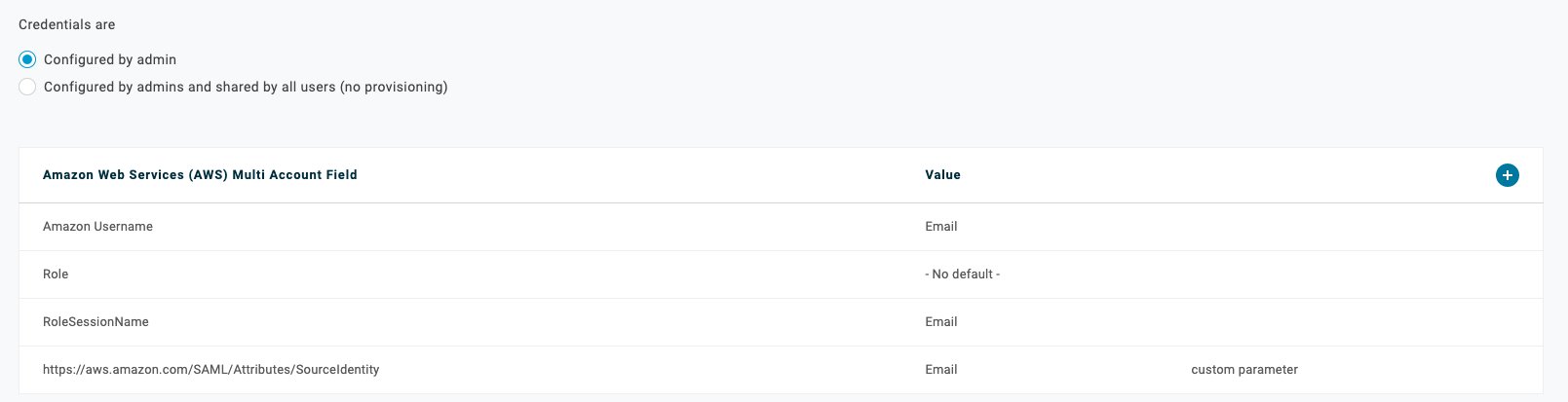
In the Attribute Mapping section line 3 as shown in Figure 4, for the application attribute https://aws.amazon.com/SAML/Attributes/RoleSessionName, enter Email (Work).
In the Attribute Mapping section as shown in Figure 4, to create line 5, choose Add a new attribute in the lower left.
In the newly added Attribute Mapping section line 5 as shown in Figure 4, add the SourceIdentity.
For Application Attribute, enter: https://aws.amazon.com/SAML/Attributes/SourceIdentity
For Identity Bridge Attribute or Literal Value, enter: SAML_SUBJECT
Choose Continue to Next Step in the lower right.
For Group Access, add your existing PingOne Directory Group to this application.
Review your setup configuration, as shown in Figure 7, and choose Finish.
Figure 7. Review mappings
Configure the SourceIdentity attribute with OneLogin integration
For the OneLogin SAML integration with AWS, you use the Amazon Web Services Multi Account application and configure an optional attribute to map as the SourceIdentity. You do this portion of the configuration in the OneLogin administrative console.
This procedure assumes that you already have a previously configured AWS and OneLogin integration. For information about how to configure the OneLogin application for AWS authentication and authorization, see the OneLogin KB article Configure SAML for Amazon Web Services (AWS) with Multiple Accounts and Roles.
After the OneLogin Multi Account application and AWS are correctly configured for SAML login, you can further customize the application to pass the SourceIdentity parameter upon login.
To change OneLogin configuration to add SourceIdentity attribute
In the OneLogin administrative console, in the Amazon Web Services Multi Account application, on the app administration page, navigate to Parameters, as shown in Figure 8.
Figure 8. OneLogin AWS Multi Account Application Configuration Parameters
To add a parameter, choose the + (plus) icon to the right of Value.
As shown in Figure 9, for Field Name enter https://aws.amazon.com/SAML/Attributes/SourceIdentity, select Include in SAML assertion, then choose Save.
Figure 9. OneLogin AWS Multi Account Application add new field
In the Edit Field page, select the default value you want to use for SourceIdentity. For the example in this blog post, for Value, select Email, then choose Save, as shown in Figure 10.
Figure 10. OneLogin AWS Multi Account Application map new field to email
After you’ve completed this procedure, review the final mapping details, as shown in Figure 11, to confirm that you see the additional parameter that will be passed into AWS through the SAML assertion.
Figure 11. OneLogin AWS Multi Account Application final mapping details
Configuring AWS IAM role trust policy
Now that the IdP configuration is complete, you can enable your AWS accounts to use SourceIdentity by modifying the IAM role trust policy.
For the workforce identity or application to be able to define their source identity when they assume IAM roles, you must first grant them permission for the sts:SetSourceIdentity action, as illustrated in the sample policy document below. This will permit the workforce identity or application to set the SourceIdentity themselves without any need for manual intervention.
To modify an AWS IAM role trust policy
Log in to the AWS Management Console for your account as a user with privileges to configure an IdP, typically an administrator.
Navigate to the AWS IAM service.
For trusted identity, choose SAML 2.0 federation.
From the SAML Provider drop down menu, select the IAM provider you created previously.
Modify the role trust policy and add the SetSourceIdentity action.
Sample policy document
This is a sample policy document attached to a role you assume when you log in to Account1 from the Okta dashboard. Edit your Account1/Role1 trust policy document and add sts:AssumeRoleWithSAML and sts:setSourceIdentity to the Action section.
Notes: The SetSourceIdentity action has to be allowed in the trust policy for assumeRole to work when the IdP is set up to pass SourceIdentity in the assertion. Future version of the sign-in URL may contain a Region code. When this occurs, you will need to modify the URL appropriately.
Policy statement
The following are examples of how the line “Federated”: “arn:aws:iam::<AccountId>:saml-provider/<IdP>” should look, based on the different IdPs specified in this post:
The following is a sample access control policy document in Account2 for Role2 that allows you to switchRole from Account1. Edit the control policy and add sts:AssumeRole and sts:SetSourceIdentity in the Action section.
Validate that the CloudTrail log entries for Account1 contain the Active Directory mapped SourceIdentity.
Use the Switch Role feature to switch to a second account Account2 (444455556666), using a role named Role2.
Create a new Amazon S3 bucket in Account2.
To summarize what you’ve done so far, you have:
Configured your corporate directory to pass a unique attribute to AWS as the source identity.
Configured a role that will persist the SourceIdentity attribute in AWS STS, which an employee will use to federate into your account.
Configured an Amazon S3 bucket that user will access.
Now you’ll observe in CloudTrail the SourceIdentity attribute that will be associated with every IAM action.
To see the SourceIdentity attribute in CloudTrail
From the your preferred IdP dashboard, select the AWS tile to log into the AWS console. The example in Figure 12 shows the Okta dashboard.
Figure 12. Login to AWS from IdP dashboard
Choose the AWS icon, which will take you to the AWS Management Console. Notice how the user has assumed the role you created earlier.
To test the SourceIdentity action, you will create a new Amazon S3 bucket.
Amazon S3 bucket names are globally unique, and the namespace is shared by all AWS accounts, so you will need to create a unique bucket name in your account. For this example, we used a bucket named DOC-EXAMPLE-BUCKET1 to validate CloudTrail log entries containing the SourceIdentity attribute.
Log into an account Account1 (111122223333) using a role named Role1.
Next, create a new Amazon S3 bucket in Account1, and validate that the Account1 CloudTrail logs entries contain the SourceIdentity attribute.
Create an Amazon S3 bucket called DOC-EXAMPLE-BUCKET1, as shown in Figure 13.
Figure 13. Create S3 bucket
In the AWS Management Console go to CloudTrail and check the log entry for bucket creation event, as shown in Figure 14.
Switch to Account2 (444455556666) using assume role, and switch to Account2/assumeRoleSourceIdentity.
Create a new Amazon S3 bucket in Account2 and validate that the Account2 CloudTrail log entries contain the SourceIdentity attribute, as shown in Figure 15.
Figure 15 – Switch role to assumeRoleSourceIdentity
Create a new Amazon S3 bucket in account2 called DOC-EXAMPLE-BUCKET2, as shown in Figure 16.
Figure 16 – Create DOC-EXAMPLE-BUCKET2 bucket while logged into account2 using assumeRoleSourceIdentity
Check the CloudTrail logs for account2 (444455556666) to see if the original SourceIdentity is logged, as shown in Figure 17.
Figure 17 – CloudTrail log entry for the above action
CloudTrail entry showing original SourceIdentity after assuming a role
You logged into Account1/Role1 and switched to Account2/Role2. All the user activities performed in AWS using the Assume Role were also logged with the original user’s sourceIdentity attribute. This makes it simple to trace user activity in CloudTrail.
Conclusion
Now that you have configured your SourceIdentity, you have made it easier for the security team of your organization to use CloudTrail logs to investigate and identify the originating identity of a user. In this post, you learned how to configure the AWS STSSourceIdentity attribute for three different popular IdPs, as well as how to configure each IdP using SAML and their optional attributes. We also provided sample control policy documents outlining how to configure the SourceIdentity for each provider. Additionally, we provide a sample policy for setting the SourceIdentity when switching roles. Lastly, the post walks through how the source identity will show in CloudTrail logs, and provides logs from two accounts to demonstrate the continuance of the source identity attribute. You can now test this capability yourself in your own environment, validate activity in your CloudTrail logs, and determine which user performed a specific action while using the assumeRole functionality.
If you have feedback about this post, submit comments in the Comments section below. If you have questions about this post, contact AWS Support.
Want more AWS Security news? Follow us on Twitter.
Andy Greenberg wrote a long article — an excerpt from his new book — on how law enforcement de-anonymized bitcoin transactions to take down a global child porn ring.
Within a few years of Bitcoin’s arrival, academic security researchers — and then companies like Chainalysis — began to tear gaping holes in the masks separating Bitcoin users’ addresses and their real-world identities. They could follow bitcoins on the blockchain as they moved from address to address until they reached one that could be tied to a known identity. In some cases, an investigator could learn someone’s Bitcoin addresses by transacting with them, the way an undercover narcotics agent might conduct a buy-and-bust. In other cases, they could trace a target’s coins to an account at a cryptocurrency exchange where financial regulations required users to prove their identity. A quick subpoena to the exchange from one of Chainalysis’ customers in law enforcement was then enough to strip away any illusion of Bitcoin’s anonymity.
Chainalysis had combined these techniques for de-anonymizing Bitcoin users with methods that allowed it to “cluster” addresses, showing that anywhere from dozens to millions of addresses sometimes belonged to a single person or organization. When coins from two or more addresses were spent in a single transaction, for instance, it revealed that whoever created that “multi-input” transaction must have control of both spender addresses, allowing Chainalysis to lump them into a single identity. In other cases, Chainalysis and its users could follow a “peel chain” — a process analogous to tracking a single wad of cash as a user repeatedly pulled it out, peeled off a few bills, and put it back in a different pocket. In those peel chains, bitcoins would be moved out of one address as a fraction was paid to a recipient and then the remainder returned to the spender at a “change” address. Distinguishing those change addresses could allow an investigator to follow a sum of money as it hopped from one address to the next, charting its path through the noise of Bitcoin’s blockchain.
Thanks to tricks like these, Bitcoin had turned out to be practically the opposite of untraceable: a kind of honeypot for crypto criminals that had, for years, dutifully and unerasably recorded evidence of their dirty deals. By 2017, agencies like the FBI, the Drug Enforcement Agency, and the IRS’s Criminal Investigation division (or IRS-CI) had traced Bitcoin transactions to carry out one investigative coup after another, very often with the help of Chainalysis.
Managing and operating asynchronous workflows can be difficult without the proper tools and architecture that puts observability, debugging, and tracing at the forefront.
Imagine getting paged outside normal work hours — users are having trouble with the application you’re responsible for, and you start diving into logs. However, they are scattered across multiple systems, and there isn’t an easy way to tie related messages together. Once you finally find useful identifiers, you may begin writing SQL queries against your production database to find out what went wrong. You’re joining tables, resolving status types, cross-referencing data manually with other systems, and by the end of it all you ask yourself why?
An upset on-call
This was the experience for us as the backend team on Prodicle Distribution, which is one of the many services offered in the suite of content production-facing applications called Prodicle.
Prodicle is one of the many applications that is at the exciting intersection of connecting the world of content productions to Netflix Studio Engineering. It enables a Production Office Coordinator to keep a Production’s cast, crew, and vendors organized and up to date with the latest information throughout the course of a title’s filming. (e.g. Netflix original series such as La Casa De Papel), as well as with Netflix Studio.
Users of Prodicle: Production Office Coordinator on their job
As the adoption of Prodicle grew over time, Productions asked for more features, which led to the system quickly evolving in multiple programming languages under different teams. When our team took ownership of Prodicle Distribution, we decided to revamp the service and expand its implementation to multiple UI clients built for web, Android and iOS.
Prodicle Distribution
Prodicle Distribution allows a production office coordinator to send secure, watermarked documents, such as scripts, to crew members as attachments or links, and track delivery. One distribution job might result in several thousand watermarked documents and links being created. If a job has 10 files and 20 recipients, then we have 10 x 20 = 200 unique watermarked documents and (optionally) links associated with them depending on the type of the Distribution job. The recipients of watermarked documents are able to access these documents and links in their email as well as in the Prodicle mobile application.
Prodicle Distribution
Our service is required to be elastic and handle bursty traffic. It also needs to handle third-party integration with Google Drive, making copies of PDFs with watermarks specific to each recipient, adding password protection, creating revocable links, generating thumbnails, and sending emails and push notifications. We are expected to process 1,000 watermarks for a single distribution in a minute, with non-linear latency growth as the number of watermarks increases. The goal is to process these documents as fast as possible and reliably deliver them to recipients while offering strong observability to both our users and internal teams.
Prodicle Distribution Requirements
Asynchronous workflow
Previously, the Distribution feature of Prodicle was treated as its own unique application. In late 2019, our team started integrating it with the rest of the ecosystem by writing a thin Java Domain graph service (DGS) to wrap the asynchronous watermarking functionality that was then in Ruby on Rails. The watermarking functionality, at the start, was a simple offering with various Google Drive integrations for storage and links. Our team was responsible for Google integrations, watermarking, bursty traffic management, and on-call support for this application. We had to traverse multiple codebases, and observability systems to debug errors and inefficiencies in the system. Things got hairy. New feature requests were adding to the maintenance burden for the team.
Initial offering of Prodicle Distribution backend
When we decided to migrate the asynchronous workflow to Java, we landed on these additional requirements: 1. We wanted a scalable service that was near real-time, 2. We wanted a workflow orchestrator with good observability for developers, and 3. We wanted to delegate the responsibility of watermarking and bursty traffic management for our asynchronous functions to appropriate teams.
Migration consideration for Prodicle Distribution’s asynchronous workflow
We evaluated what it would take to do this ourselves or rely on the offerings from our platform teams — Conductor and one of the new offerings Cosmos. Even though Cosmos was developed for asynchronous media processing, we worked with them to expand to generic file processing and tune their workflow platform for our near real-time use case. Early prototypes and load tests validated that the offering could meet our needs. We leaned into Cosmos because of the low variance in latency through the system, separation of concerns between the API, workflow, and the function systems, ease of load testing, customizable API layer and notifications, support for File I/O abstractions and elastic functions. Another benefit was their observability portal and its capabilities with search. We also migrated the ownership of watermarking to another internal team to focus on developing and supporting additional features.
Current architecture of Prodicle Distribution on Cosmos
With Cosmos, we are well-positioned to expand to future use cases like watermarking on images and videos. The Cosmos team is dedicated to improving features and functionality over the next year to make observations of our async workflows even better. It is great to have a team that will be improving the platform in the background as we continue our application development. We expect the performance and scaling to continue to get better without much effort on our part. We also expect other services to move some of their processing functionality into Cosmos, which makes integrations even easier because services can expose a function within the platform instead of GRPC or REST endpoints. The more services move to Cosmos, the bigger the value proposition becomes.
Deployed to Production for Productions
With productions returning to work in the midst of a global pandemic, the adoption of Prodicle Distribution has grown 10x, between June 2020 and April 2021. Starting January 2021 we did an incremental release of Prodicle Distribution on Cosmos and completed the migration in April 2021. We now support hundreds of productions, with tens of thousands of Distribution jobs, and millions of watermarks every month.
With our migration of Prodicle Distribution to Cosmos, we are able to use their observability portal called Nirvana to debug our workflow and bottlenecks.
Observing Prodicle Distribution on Cosmos in Nirvana
Now that we have a platform team dedicated to the management of our async infrastructure and watermarking, our team can better maintain and support the distribution of documents. Since our migration, the number of support tickets has decreased. It is now easier for the on-call engineer and the developers to find the associated logs and traces while visualizing the state of the asynchronous workflow and data in the whole system.
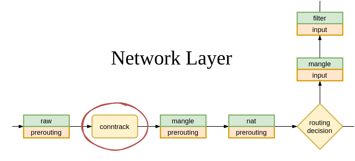
We have been working with conntrack, the connection tracking layer in the Linux kernel, for years. And yet, despite the collected know-how, questions about its inner workings occasionally come up. When they do, it is hard to resist the temptation to go digging for answers.
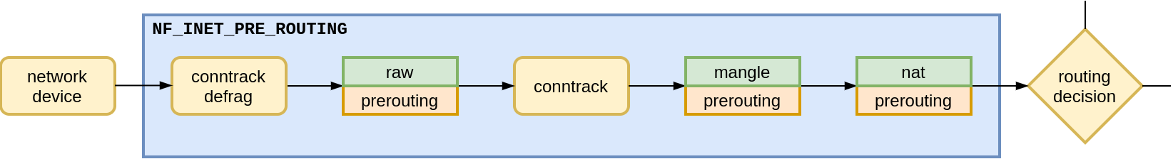
We already know from last time that conntrack is in charge of tracking incoming and outgoing network traffic. By running conntrack -L we can inspect existing network flows, or as conntrack calls them, connections.
So if we spin up a toy VM, connect to it over SSH, and inspect the contents of the conntrack table, we will see…
$ vagrant init fedora/33-cloud-base
$ vagrant up
…
$ vagrant ssh
Last login: Sun Jan 31 15:08:02 2021 from 192.168.122.1
[vagrant@ct-vm ~]$ sudo conntrack -L
conntrack v1.4.5 (conntrack-tools): 0 flow entries have been shown.
… nothing!
Even though the conntrack kernel module is loaded:
Hold on a minute. Why is the SSH connection to the VM not listed in conntrack entries? SSH is working. With each keystroke we are sending packets to the VM. But conntrack doesn’t register it.
Isn’t conntrack an integral part of the network stack that sees every packet passing through it? 🤔
Clearly everything we learned about conntrack last time is not the whole story.
Calling into conntrack
Our little experiment with SSH’ing into a VM begs the question — how does conntrack actually get notified about network packets passing through the stack?
We can walk the receive path step by step and we won’t find any direct calls into the conntrack code in either the IPv4 or IPv6 stack. Conntrack does not interface with the network stack directly.
Instead, it relies on the Netfilter framework, and its set of hooks baked into in the stack:
Netfilter users, like conntrack, can register callbacks with it. Netfilter will then run all registered callbacks when its hook processes a network packet.
For the INET family, that is IPv4 and IPv6, there are five Netfilter hooks to choose from:
Which ones does conntrack use? We will get to that in a moment.
First, let’s focus on the trigger. What makes conntrack register its callbacks with Netfilter?
The SSH connection doesn’t show up in the conntrack table just because the module is loaded. We already saw that. This means that conntrack doesn’t register its callbacks with Netfilter at module load time.
Or at least, it doesn’t do it by default. Since Linux v5.1 (May 2019) the conntrack module has the enable_hooks parameter, which causes conntrack to register its callbacks on load:
Nice! The conntrack table now contains an entry for our SSH session.
The Netfilter hook notified conntrack about SSH session packets passing through the stack.
Now that we know how conntrack gets called, we can go back to our question — can we observe a TCP SYN packet dropped by the firewall with conntrack?
Listing Netfilter hooks
That is easy to check:
Add a rule to drop anything coming to port tcp/25702
[vagrant@ct-vm ~]$ sudo iptables -t filter -A INPUT -p tcp --dport 2570 -j DROP
2) Connect to the VM on port tcp/2570 from the outside
host $ nc -w 1 -z 192.168.122.204 2570
3) List conntrack table entries
[vagrant@ct-vm ~]$ sudo conntrack -L
tcp      6 431999 ESTABLISHED src=192.168.122.204 dst=192.168.122.1 sport=22 dport=34858 src=192.168.122.1 dst=192.168.122.204 sport=34858 dport=22 [ASSURED] mark=0 secctx=system_u:object_r:unlabeled_t:s0 use=1
conntrack v1.4.5 (conntrack-tools): 1 flow entries have been shown.
No new entries. Conntrack didn’t record a new flow for the dropped SYN.
But did it process the SYN packet? To answer that we have to find out which callbacks conntrack registered with Netfilter.
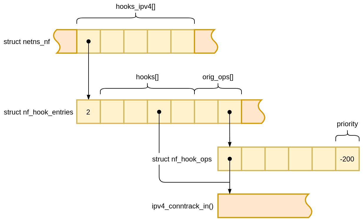
Netfilter keeps track of callbacks registered for each hook in instances of struct nf_hook_entries. We can reach these objects through the Netfilter state (struct netns_nf), which lives inside network namespace (struct net).
struct nf_hook_entries, if you look at its definition, is a bit of an exotic construct. A glance at how the object size is calculated during its allocation gives a hint about its memory layout:
It’s an element count, followed by two arrays glued together, and some RCU-related state which we’re going to ignore. The two arrays have the same size, but hold different kinds of values.
We can walk the second array, holding pointers to struct nf_hook_ops, to discover the registered callbacks and their priority. Priority determines the invocation order.
With drgn, a programmable C debugger tailored for the Linux kernel, we can locate the Netfilter state in kernel memory, and walk its contents relatively easily. Given we know what we are looking for.
[vagrant@ct-vm ~]$ sudo drgn
drgn 0.0.8 (using Python 3.9.1, without libkdumpfile)
…
>>> pre_routing_hook = prog['init_net'].nf.hooks_ipv4[0]
>>> for i in range(0, pre_routing_hook.num_hook_entries):
...     pre_routing_hook.hooks[i].hook
...
(nf_hookfn *)ipv4_conntrack_defrag+0x0 = 0xffffffffc092c000
(nf_hookfn *)ipv4_conntrack_in+0x0 = 0xffffffffc093f290
>>>
Neat! We have a way to access Netfilter state.
Let’s take it to the next level and list all registered callbacks for each Netfilter hook (using less than 100 lines of Python):
The output from our script shows that conntrack has two callbacks registered with the PRE_ROUTING hook – ipv4_conntrack_defrag and ipv4_conntrack_in. But are they being called?
We expect that when the Netfilter PRE_ROUTING hook processes a TCP SYN packet, it will invoke ipv4_conntrack_defrag and then ipv4_conntrack_in callbacks.
To confirm it we will put to use the tracing powers of BPF 🐝. BPF programs can run on entry to functions. These kinds of programs are known as BPF kprobes. In our case we will attach BPF kprobes to conntrack callbacks.
Usually, when working with BPF, we would write the BPF program in C and use clang -target bpf to compile it. However, for tracing it will be much easier to use bpftrace. With bpftrace we can write our BPF kprobe program in a high-level language inspired by AWK:
What does this program do? It is roughly an equivalent of a tcpdump filter:
dst port 2570 and tcp[tcpflags] & tcp-syn != 0
But only for packets passing through conntrack PRE_ROUTING callbacks.
(If you haven’t used bpftrace, it comes with an excellent reference guide and gives you the ability to explore kernel data types on the fly with bpftrace -lv 'struct iphdr'.)
Let’s run the tracing program while we connect to the VM from the outside (nc -z 192.168.122.204 2570):
[vagrant@ct-vm ~]$ sudo bpftrace /vagrant/tools/trace-conntrack-prerouting.bt
Attaching 3 probes...
Tracing conntrack prerouting callbacks... Hit Ctrl-C to quit
13:22:56 192.168.122.1:33254 > 192.168.122.204:2570 tcp syn ipv4_conntrack_defrag
13:22:56 192.168.122.1:33254 > 192.168.122.204:2570 tcp syn ipv4_conntrack_in
^C

[vagrant@ct-vm ~]$
Conntrack callbacks have processed the TCP SYN packet destined to tcp/2570.
But if conntrack saw the packet, why is there no corresponding flow entry in the conntrack table?
Going down the rabbit hole
What actually happens inside the conntrack PRE_ROUTING callbacks?
To find out, we can trace the call chain that starts on entry to the conntrack callback. The function_graph tracer built into the Ftrace framework is perfect for this task.
But because all incoming traffic goes through the PRE_ROUTING hook, including our SSH connection, our trace will be polluted with events from SSH traffic. To avoid that, let’s switch from SSH access to a serial console.
When using libvirt as the Vagrant provider, you can connect to the serial console with virsh:
host $ virsh -c qemu:///session list
 Id   Name                State
-----------------------------------
 1    conntrack_default   running

host $ virsh -c qemu:///session console conntrack_default
Once connected to the console and logged into the VM, we can record the call chain using the trace-cmd wrapper for Ftrace:
[vagrant@ct-vm ~]$ sudo trace-cmd start -p function_graph -g ipv4_conntrack_defrag -g ipv4_conntrack_in
  plugin 'function_graph'
[vagrant@ct-vm ~]$ # … connect from the host with `nc -z 192.168.122.204 2570` …
[vagrant@ct-vm ~]$ sudo trace-cmd stop
[vagrant@ct-vm ~]$ sudo cat /sys/kernel/debug/tracing/trace
# tracer: function_graph
#
# CPU  DURATION                  FUNCTION CALLS
# |     |   |                     |   |   |   |
 1)   1.219 us    |  finish_task_switch();
 1)   3.532 us    |  ipv4_conntrack_defrag [nf_defrag_ipv4]();
 1)               |  ipv4_conntrack_in [nf_conntrack]() {
 1)               |    nf_conntrack_in [nf_conntrack]() {
 1)   0.573 us    |      get_l4proto [nf_conntrack]();
 1)               |      nf_ct_get_tuple [nf_conntrack]() {
 1)   0.487 us    |        nf_ct_get_tuple_ports [nf_conntrack]();
 1)   1.564 us    |      }
 1)   0.820 us    |      hash_conntrack_raw [nf_conntrack]();
 1)   1.255 us    |      __nf_conntrack_find_get [nf_conntrack]();
 1)               |      init_conntrack.constprop.0 [nf_conntrack]() {  ❷
 1)   0.427 us    |        nf_ct_invert_tuple [nf_conntrack]();
 1)               |        __nf_conntrack_alloc [nf_conntrack]() {      ❶
                             …
 1)   3.680 us    |        }
                           …
 1) + 15.847 us   |      }
                         …
 1) + 34.595 us   |    }
 1) + 35.742 us   |  }
 …
[vagrant@ct-vm ~]$
What catches our attention here is the allocation, __nf_conntrack_alloc() (❶), inside init_conntrack() (❷). __nf_conntrack_alloc() creates a struct nf_conn object which represents a tracked connection.
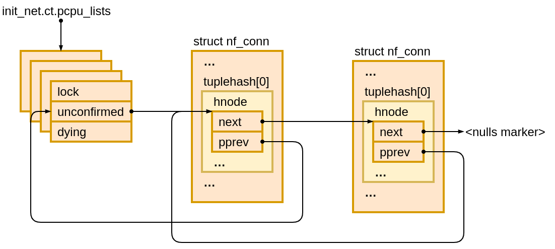
This object is not created in vain. A glance at init_conntrack()source shows that it is pushed onto a list of unconfirmed connections3.
What does it mean that a connection is unconfirmed? As conntrack(8) man page explains:
unconfirmed:
       This table shows new entries, that are not yet inserted into the
       conntrack table. These entries are attached to packets that  are
       traversing  the  stack, but did not reach the confirmation point
       at the postrouting hook.
Perhaps we have been looking for our flow in the wrong table? Does the unconfirmed table have a record for our dropped TCP SYN?
Pulling the rabbit out of the hat
I have bad news…
[vagrant@ct-vm ~]$ sudo conntrack -L unconfirmed
conntrack v1.4.5 (conntrack-tools): 0 flow entries have been shown.
[vagrant@ct-vm ~]$
The flow is not present in the unconfirmed table. We have to dig deeper.
Let’s for a moment assume that a struct nf_conn object was added to the unconfirmed list. If the list is now empty, then the object must have been removed from the list before we inspected its contents.
Has an entry been removed from the unconfirmed table? What function removes entries from the unconfirmed table?
It turns out that nf_ct_add_to_unconfirmed_list() which init_conntrack() invokes, has its opposite defined just right beneath it – nf_ct_del_from_dying_or_unconfirmed_list().
It is worth a shot to check if this function is being called, and if so, from where. For that we can again use a BPF tracing program, attached to function entry. However, this time our program will record a kernel stack trace:
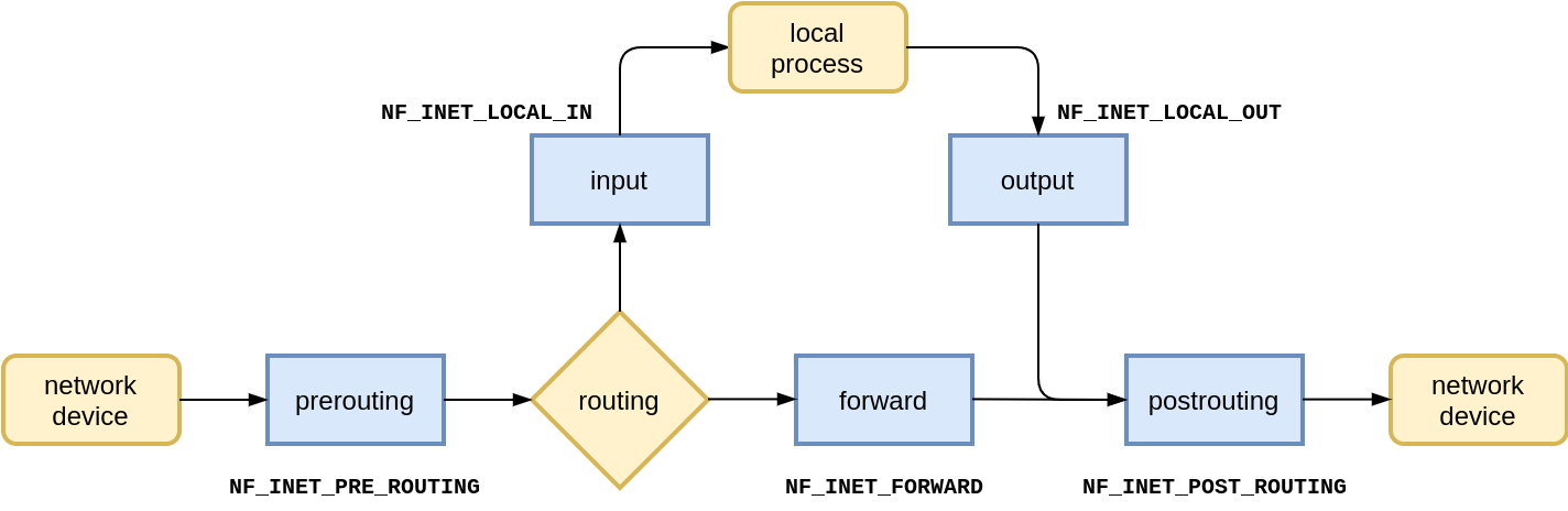
Bingo. The conntrack delete function was called, and the captured stack trace shows that on local delivery path (❶), where LOCAL_IN Netfilter hook runs (❷), the packet is destroyed (❸). Conntrack must be getting called when sk_buff (the packet and its metadata) is destroyed. This causes conntrack to remove the unconfirmed flow entry (❹).
It makes sense. After all we have a DROP rule in the filter/INPUT chain. And that iptables -j DROP rule has a significant side effect. It cleans up an entry in the conntrack unconfirmed table!
This explains why we can’t observe the flow in the unconfirmed table. It lives for only a very short period of time.
Not convinced? You don’t have to take my word for it. I will prove it with a dirty trick!
Making the rabbit disappear, or actually appear
If you recall the output from list-nf-hooks that we’ve seen earlier, there is another conntrack callback there – ipv4_confirm, which I have ignored:
ipv4_confirm is “the confirmation point” mentioned in the conntrack(8) man page. When a flow gets confirmed, it is moved from the unconfirmed table to the main conntrack table.
The callback is registered with a “weird” priority – 2,147,483,647. It’s the maximum positive value of a 32-bit signed integer can hold, and at the same time, the lowest possible priority a callback can have.
This ensures that the ipv4_confirm callback runs last. We want the flows to graduate from the unconfirmed table to the main conntrack table only once we know the corresponding packet has made it through the firewall.
Luckily for us, it is possible to have more than one callback registered with the same priority. In such cases, the order of registration matters. We can put that to use. Just for educational purposes.
Good old iptables won’t be of much help here. Its Netfilter callbacks have hard-coded priorities which we can’t change. But nftables, the iptablessuccessor, is much more flexible in this regard. With nftables we can create a rule chain with arbitrary priority.
So this time, let’s use nftables to install a filter rule to drop traffic to port tcp/2570. The trick, though, is to register our chain before conntrack registers itself. This way our filter will run last.
First, delete the tcp/2570 drop rule in iptables and unregister conntrack.
vm # iptables -t filter -F
vm # rmmod nf_conntrack_netlink nf_conntrack
Then add tcp/2570 drop rule in nftables, with lowest possible priority.
vm # nft add table ip my_table
vm # nft add chain ip my_table my_input { type filter hook input priority 2147483647 \; }
vm # nft add rule ip my_table my_input tcp dport 2570 counter drop
vm # nft -a list ruleset
table ip my_table { # handle 1
        chain my_input { # handle 1
                type filter hook input priority 2147483647; policy accept;
                tcp dport 2570 counter packets 0 bytes 0 drop # handle 4
        }
}
Finally, re-register conntrack hooks.
vm # modprobe nf_conntrack enable_hooks=1
The registered callbacks for the LOCAL_IN hook now look like this:
vm # conntrack -L
tcp      6 115 SYN_SENT src=192.168.122.1 dst=192.168.122.204 sport=54868 dport=2570 [UNREPLIED] src=192.168.122.204 dst=192.168.122.1 sport=2570 dport=54868 mark=0 secctx=system_u:object_r:unlabeled_t:s0 use=1
conntrack v1.4.5 (conntrack-tools): 1 flow entries have been shown.
We have fooled conntrack 💥
Conntrack promoted the flow from the unconfirmed to the main conntrack table despite the fact that the firewall dropped the packet. We can observe it.
Outro
Conntrack processes every received packet4 and creates a flow for it. A flow entry is always created even if the packet is dropped shortly after. The flow might never be promoted to the main conntrack table and can be short lived.
However, this blog post is not really about conntrack. Its internals have been covered by magazines, papers, books, and on other blogs long before. We probably could have learned elsewhere all that has been shown here.
For us, conntrack was really just an excuse to demonstrate various ways to discover the inner workings of the Linux network stack. As good as any other.
Today we have powerful introspection tools like drgn, bpftrace, or Ftrace, and a cross referencer to plow through the source code, at our fingertips. They help us look under the hood of a live operating system and gradually deepen our understanding of its workings.
I have to warn you, though. Once you start digging into the kernel, it is hard to stop…
……….. 1Actually since Linux v5.10 (Dec 2020) there is an additional Netfilter hook for the INET family named NF_INET_INGRESS. The new hook type allows users to attach nftables chains to the Traffic Control ingress hook. 2Why did I pick this port number? Because 2570 = 0x0a0a. As we will see later, this saves us the trouble of converting between the network byte order and the host byte order. 3To be precise, there are multiple lists of unconfirmed connections. One per each CPU. This is a common pattern in the kernel. Whenever we want to prevent CPUs from contending for access to a shared state, we give each CPU a private instance of the state. 4Unless we explicitly exclude it from being tracked with iptables -j NOTRACK.
The collective thoughts of the interwebz
Manage Consent
To provide the best experiences, we use technologies like cookies to store and/or access device information. Consenting to these technologies will allow us to process data such as browsing behavior or unique IDs on this site. Not consenting or withdrawing consent, may adversely affect certain features and functions.
Functional
Always active
The technical storage or access is strictly necessary for the legitimate purpose of enabling the use of a specific service explicitly requested by the subscriber or user, or for the sole purpose of carrying out the transmission of a communication over an electronic communications network.
Preferences
The technical storage or access is necessary for the legitimate purpose of storing preferences that are not requested by the subscriber or user.
Statistics
The technical storage or access that is used exclusively for statistical purposes.The technical storage or access that is used exclusively for anonymous statistical purposes. Without a subpoena, voluntary compliance on the part of your Internet Service Provider, or additional records from a third party, information stored or retrieved for this purpose alone cannot usually be used to identify you.
Marketing
The technical storage or access is required to create user profiles to send advertising, or to track the user on a website or across several websites for similar marketing purposes.


