All posts by Dhiraj Thakur

Build a real-time GDPR-aligned Apache Iceberg data lake

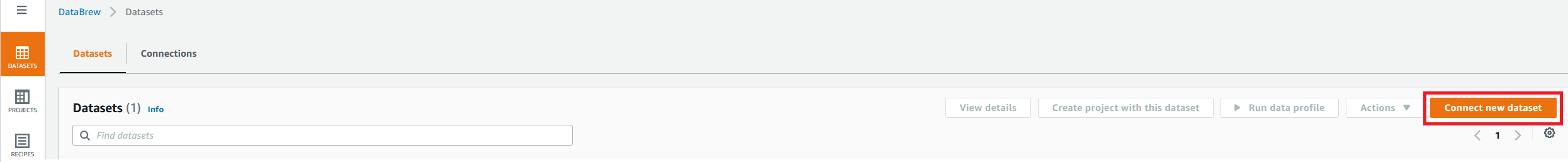
Post Syndicated from Dhiraj Thakur original https://aws.amazon.com/blogs/big-data/build-a-real-time-gdpr-aligned-apache-iceberg-data-lake/

Data lakes are a popular choice for today’s organizations to store their data around their business activities. As a best practice of a data lake design, data should be immutable once stored. But regulations such as the General Data Protection Regulation (GDPR) have created obligations for data operators who must be able to erase or update personal data from their data lake when requested.

A data lake built on AWS uses Amazon Simple Storage Service (Amazon S3) as its primary storage environment. When a customer asks to erase or update private data, the data lake operator needs to find the required objects in Amazon S3 that contain the required data and take steps to erase or update that data. This activity can be a complex process for the following reasons:

  • Data lakes may contain many S3 objects (each may contain multiple rows), and often it’s difficult to find the object containing the exact data that needs to be erased or personally identifiable information (PII) to be updated as per the request
  • By nature, S3 objects are immutable and therefore applying direct row-based transactions like DELETE or UPDATE isn’t possible

To handle these situations, a transactional feature on S3 objects is required, and frameworks such as Apache Hudi or Apache Iceberg provide you the transactional feature for upserts in Amazon S3.

AWS contributed the Apache Iceberg integration with the AWS Glue Data Catalog, which enables you to use open-source data computation engines like Apache Spark with Iceberg on AWS Glue. In 2022, Amazon Athena announced support of Iceberg, enabling transaction queries on S3 objects.

In this post, we show you how to stream real-time data to an Iceberg table in Amazon S3 using AWS Glue streaming and perform transactions using Amazon Athena for deletes and updates. We use a serverless mechanism for this implementation, which requires minimum operational overhead to manage and fine-tune various configuration parameters, and enables you to extend your use case to ACID operations beyond the GDPR.

Solution overview

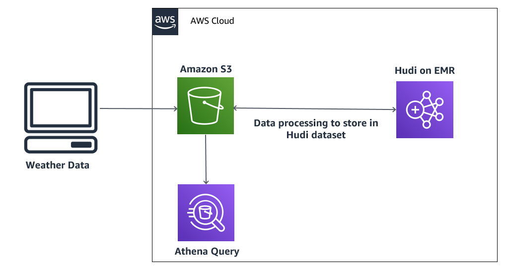
We used the Amazon Kinesis Data Generator (KDG) to produce synthetic streaming data in Amazon Kinesis Data Streams and then processed the streaming input data using AWS Glue streaming to store the data in Amazon S3 in Iceberg table format. As part of the customer’s request, we ran delete and update statements using Athena with Iceberg support.

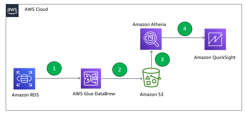
The following diagram illustrates the solution architecture.

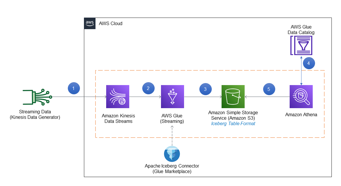
The solution workflow consists of the following steps:

  1. Streaming data is generated in JSON format using the KDG template and inserted into Kinesis Data Streams.
  2. An AWS Glue streaming job is connected to Kinesis Data Streams to process the data using the Iceberg connector.
  3. The streaming job output is stored in Amazon S3 in Iceberg table format.
  4. Athena uses the AWS Glue Data Catalog to store and retrieve table metadata for the Amazon S3 data in Iceberg format.
  5. Athena interacts with the Data Catalog tables in Iceberg format for transactional queries required for GDPR.

The codebase required for this post is available in the GitHub repository.

Prerequisites

Before starting the implementation, make sure the following prerequisites are met:

Deploy resources using AWS CloudFormation

Complete the following steps to deploy your solution resources:

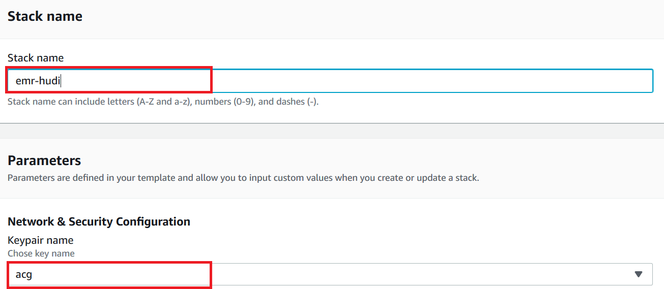
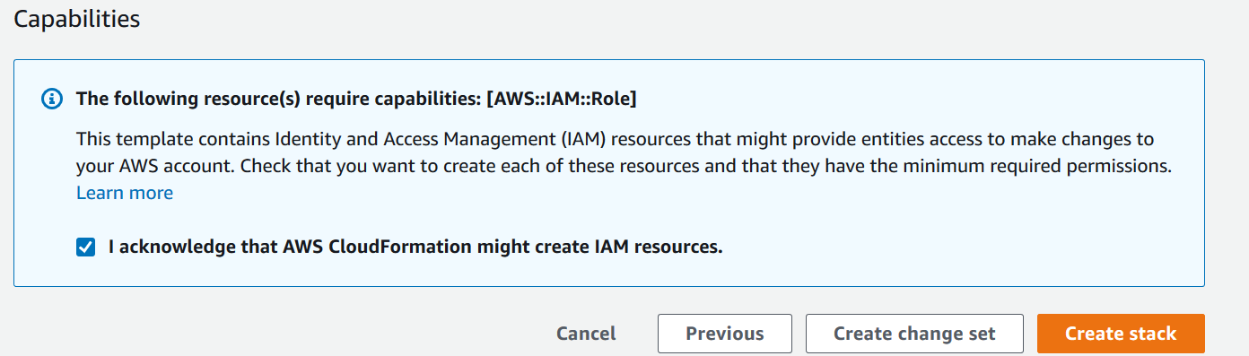
  1. After you sign in to your AWS account, launch the CloudFormation template by choosing Launch Stack:
  2. For Stack name, enter a name.
  3. For Username, enter the user name for the KDG.
  4. For Password, enter the password for the KDG (this must be at least six alphanumeric characters, and contain at least one number).
  5. For IAMGlueStreamingJobRoleName, enter a name for the IAM role used for the AWS Glue streaming job.
  6. Choose Next and create your stack.

This CloudFormation template configures the following resources in your account:

  • An S3 bucket named streamingicebergdemo-XX (note that the XX part is a random unique number to make the S3 bucket name unique)
  • An IAM policy and role
  • The KDG URL used for creating synthetic data
  1. After you complete the setup, go to the Outputs tab of the CloudFormation stack to get the S3 bucket name, AWS Glue job execution role (as per your input), and KDG URL.
  2. Before proceeding with the demo, create a folder named custdata under the created S3 bucket.

Create a Kinesis data stream

We use Kinesis Data Streams to create a serverless streaming data service that is built to handle millions of events with low latency. The following steps guide you on how to create the data stream in the us-east-1 Region:

  1. Log in to the AWS Management Console.
  2. Navigate to Kinesis console (make sure the Region is us-east-1).
  3. Select Kinesis Data Streams and choose Create data stream.
  4. For Data stream name, enter demo-data-stream.
  5. For this post, we select On-demand as the Kinesis data stream capacity mode.

On-demand mode works to eliminate the need for provisioning and managing the capacity for streaming data. However, you can implement this solution with Kinesis Data Streams in provisioned mode as well.

  1. Choose Create data stream.
  2. Wait for successful creation of demo-data-stream and for it to be in Active status.

Set up the Kinesis Data Generator

To create a sample streaming dataset, we use the KDG URL generated on the CloudFormation stack Outputs tab and log in with the credentials used in the parameters for the CloudFormation template. For this post, we use the following template to generate sample data in the demo-data-stream Kinesis data stream.

  1. Log in to the KDG URL with the user name and password you supplied during stack creation.
  2. Change the Region to us-east-1.
  3. Select the Kinesis data stream demo-data-stream.
  4. For Records per second, choose Constant and enter 100 (it can be another number, depending on the rate of record creation).
  5. On the Template 1 tab, enter the KDG data generation template:
{
"year": "{{random.number({"min":2000,"max":2022})}}",
"month": "{{random.number({"min":1,"max":12})}}",
"day": "{{random.number({"min":1,"max":30})}}",
"hour": "{{random.number({"min":0,"max":24})}}",
"minute": "{{random.number({"min":0,"max":60})}}",
"customerid": {{random.number({"min":5023,"max":59874})}},
"firstname" : "{{name.firstName}}",
"lastname" : "{{name.lastName}}",
"dateofbirth" : "{{date.past(70)}}",
"city" : "{{address.city}}",
"buildingnumber" : {{random.number({"min":63,"max":947})}},
"streetaddress" : "{{address.streetAddress}}",
"state" : "{{address.state}}",
"zipcode" : "{{address.zipCode}}",
"country" : "{{address.country}}",
"countrycode" : "{{address.countryCode}}",
"phonenumber" : "{{phone.phoneNumber}}",
"productname" : "{{commerce.productName}}",
"transactionamount": {{random.number(
{
"min":10,
"max":150
}
)}}
}
  1. Choose Test template to test the sample records.
  2. When the testing is correct, choose Send data.

This will start sending 100 records per second in the Kinesis data stream. (To stop sending data, choose Stop Sending Data to Kinesis.)

Integrate Iceberg with AWS Glue

To add the Apache Iceberg Connector for AWS Glue, complete the following steps. The connector is free to use and supports AWS Glue 1.0, 2.0, and 3.0.

  1. On the AWS Glue console, choose AWS Glue Studio in the navigation pane.
  2. In the navigation pane, navigate to AWS Marketplace.
  3. Search for and choose Apache Iceberg Connector for AWS Glue.
  4. Choose Accept Terms and Continue to Subscribe.
  5. Choose Continue to Configuration.
  6. For Fulfillment option, choose your AWS Glue version.
  7. For Software version, choose the latest software version.
  8. Choose Continue to Launch.
  9. Under Usage Instructions, choose the link to activate the connector.
  10. Enter a name for the connection, then choose Create connection and activate the connector.
  11. Verify the new connector on the AWS Glue Studio Connectors.

Create the AWS Glue Data Catalog database

The AWS Glue Data Catalog contains references to data that is used as sources and targets of your extract, transform, and load (ETL) jobs in AWS Glue. To create your data warehouse or data lake, you must catalog this data. The AWS Glue Data Catalog is an index to the location and schema of your data. You use the information in the Data Catalog to create and monitor your ETL jobs.

For this post, we create a Data Catalog database named icebergdemodb containing the metadata information of a table named customer, which will be queried through Athena.

  1. On the AWS Glue console, choose Databases in the navigation pane.
  2. Choose Add database.
  3. For Database name, enter icebergdemodb.

This creates an AWS Glue database for metadata storage.

Create a Data Catalog table in Iceberg format

In this step, we create a Data Catalog table in Iceberg table format.

  1. On the Athena console, create an Athena workgroup named demoworkgroup for SQL queries.
  2. Choose Athena engine version 3 for Query engine version.

For more information about Athena versions, refer to Changing Athena engine versions.

  1. Enter the S3 bucket location for Query result configuration under Additional configurations.
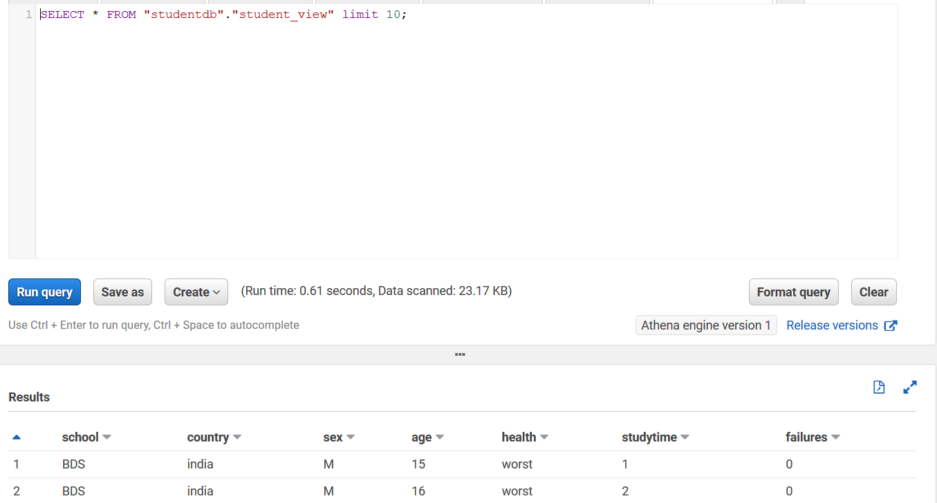
  2. Open the Athena query editor and choose demoworkgroup.
  3. Choose the database icebergdemodb.
  4. Enter and run the following DDL to create a table pointing to the Data Catalog database icerbergdemodb. Note that the TBLPROPERTIES section mentions ICEBERG as the table type and LOCATION points to the S3 folder (custdata) URI created in earlier steps. This DDL command is available on the GitHub repo.
CREATE TABLE icebergdemodb.customer(
year string,
month string,
day string,
hour string,
minute string,
customerid string,
firstname string,
lastname string,
dateofbirth string,
city string,
buildingnumber string,
streetaddress string,
state string,
zipcode string,
country string,
countrycode string,
phonenumber string,
productname string,
transactionamount int)
LOCATION '<S3 Location URI>'
TBLPROPERTIES (
'table_type'='ICEBERG',
'format'='parquet',
'write_target_data_file_size_bytes'='536870912',
'optimize_rewrite_delete_file_threshold'='10'
);

After you run the command successfully, you can see the table customer in the Data Catalog.

Create an AWS Glue streaming job

In this section, we create the AWS Glue streaming job, which fetches the record from the Kinesis data stream using the Spark script editor.

  1. On the AWS Glue console, choose Jobs (new) in the navigation pane.
  2. For Create job¸ select Spark script editor.
  3. For Options¸ select Create a new script with boilerplate code.
  4. Choose Create.
  5. Enter the code available in the GitHub repo in the editor.

The sample code keeps appending data in the target location by fetching records from the Kinesis data stream.

  1. Choose the Job details tab in the query editor.
  2. For Name, enter Demo_Job.
  3. For IAM role¸ choose demojobrole.
  4. For Type, choose Spark Streaming.
  5. For Glue Version, choose Glue 3.0.
  6. For Language, choose Python 3.
  7. For Worker type, choose G 0.25X.
  8. Select Automatically scale the number of workers.
  9. For Maximum number of workers, enter 5.
  10. Under Advanced properties, select Use Glue Data Catalog as the Hive metastore.
  11. For Connections, choose the connector you created.
  12. For Job parameters, enter the following key pairs (provide your S3 bucket and account ID):
Key Value
--iceberg_job_catalog_warehouse s3://streamingicebergdemo-XX/custdata/
--output_path s3://streamingicebergdemo-XX
--kinesis_arn arn:aws:kinesis:us-east-1:<AWS Account ID>:stream/demo-data-stream
--user-jars-first True

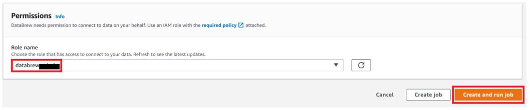
  1. Choose Run to start the AWS Glue streaming job.
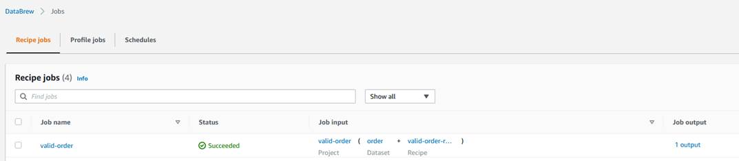
  2. To monitor the job, choose Monitoring in the navigation pane.
  3. Select Demo_Job and choose View run details to check the job run details and Amazon CloudWatch logs.

Run GDPR use cases on Athena

In this section, we demonstrate a few use cases that are relevant to GDPR alignment with the user data that’s stored in Iceberg format in the Amazon S3-based data lake as implemented in the previous steps. For this, let’s consider that the following requests are being initiated in the workflow to comply with the regulations:

  • Delete the records for the input customerid (for example, 59289)
  • Update phonenumber for the customerid (for example, 51842)

The IDs used in this example are samples only because they were created through the KDG template used earlier, which creates sample data. You can search for IDs in your implementation by querying through the Athena query editor. The steps remain the same.

Delete data by customer ID

Complete the following steps to fulfill the first use case:

  1. On the Athena console, and make sure icebergdemodb is chosen as the database.
  2. Open the query editor.
  3. Enter the following query using a customer ID and choose Run:
SELECT count(*)
FROM icebergdemodb.customer
WHERE customerid = '59289';

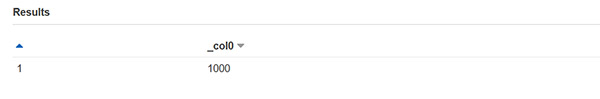
This query gives the count of records for the input customerid before delete.

  1. Enter the following query with the same customer ID and choose Run:
MERGE INTO icebergdemodb.customer trg
USING (SELECT customerid
FROM icebergdemodb.customer
WHERE customerid = '59289') src
ON (trg.customerid = src.customerid)
WHEN MATCHED
THEN DELETE;

This query deletes the data for the input customerid as per the workflow generated.

  1. Test if there is data with the customer ID using a count query.

The count should be 0.

Update data by customer ID

Complete the following steps to test the second use case:

  1. On the Athena console, make sure icebergdemodb is chosen as the database.
  2. Open the query editor.
  3. Enter the following query with a customer ID and choose Run.
SELECT customerid, phonenumber
FROM icebergdemodb.customer
WHERE customerid = '51936';

This query gives the value for phonenumber before update.

  1. Run the following query to update the required columns:
MERGE INTO icebergdemodb.customer trg
USING (SELECT customerid
FROM icebergdemodb.customer
WHERE customerid = '51936') src
ON (trg.customerid = src.customerid)
WHEN MATCHED
THEN UPDATE SET phonenumber = '000';

This query updates the data to a dummy value.

  1. Run the SELECT query to check the update.

You can see the data is updated correctly.

Vacuum table

A good practice is to run the VACUUM command periodically on the table because operations like INSERT, UPDATE, DELETE, and MERGE will take place on the Iceberg table. See the following code:

VACUUM icebergdemodb.customer;

Considerations

The following are a few considerations to keep in mind for this implementation:

Clean up

Complete the following steps to clean up the resources you created for this post:

    1. Delete the custdata folder in the S3 bucket.
    2. Delete the CloudFormation stack.
    3. Delete the Kinesis data stream.
    4. Delete the S3 bucket storing the data.
    5. Delete the AWS Glue job and Iceberg connector.
    6. Delete the AWS Glue Data Catalog database and table.
    7. Delete the Athena workgroup.
    8. Delete the IAM roles and policies.

Conclusion

This post explained how you can use the Iceberg table format on Athena to implement GDPR use cases like data deletion and data upserts as required, when streaming data is being generated and ingested through AWS Glue streaming jobs in Amazon S3.

The operations for the Iceberg table that we demonstrated in this post aren’t all of the data operations that Iceberg supports. Refer to the Apache Iceberg documentation for details on various operations.


About the Authors

Dhiraj Thakur is a Solutions Architect with Amazon Web Services. He works with AWS customers and partners to provide guidance on enterprise cloud adoption, migration, and strategy. He is passionate about technology and enjoys building and experimenting in the analytics and AI/ML space.

Rajdip Chaudhuri is Solutions Architect with Amazon Web Services specializing in data and analytics. He enjoys working with AWS customers and partners on data and analytics requirements. In his spare time, he enjoys soccer.

Announcing the AWS Well-Architected Data Analytics Lens

Post Syndicated from Dhiraj Thakur original https://aws.amazon.com/blogs/big-data/announcing-the-aws-well-architected-data-analytics-lens/

We are delighted to announce the release of the Data Analytics Lens. The lens consists of a lens whitepaper and an AWS-created lens available in the Lens Catalog of the AWS Well-Architected Tool. The AWS Well-Architected Framework provides a consistent approach to evaluate architectures and implement scalable designs. With the AWS Well-Architected Framework, cloud architects, system architects, engineers, and developers can build secure, high-performance, resilient, and efficient infrastructure for their applications and workloads.

Using the Lens in the Tool’s Lens Catalog, you can directly assess your Analytics workload in the console, and produce a set of actionable results for customized improvement plans recommended by the Tool.

The updated Data Analytics Lens outlines the most up-to-date steps for performing an AWS Well-Architected review that empowers you to assess and identify technical risks of your data analytics platforms. The new whitepaper and Lens cover multiple analytics use cases and scenarios, and provide comprehensive guidance to help you design your analytics applications in accordance with AWS best practices.

The new Data Analytics Lens offers implementation guidance you can use to deliver secure, high performance and reliable workloads, all with an eye toward maintaining cost-effectiveness and sustainability.

For more information on AWS Well-Architected Lenses, refer to AWS Well-Architected.

What’s new in the Data Analytics Lens?

The Data Analytics Lens is a collection of customer-proven design principles, best practices, and prescriptive guidance to help you adopt a cloud-centered approach to running analytics on AWS. These recommendations are based on insights that AWS has gathered from customers, AWS Partners, the field, and our own analytics technical specialist communities.

This version covers the following topics:

  • New Lens for the Well-Architected Tool in the Lens Catalog
  • New Data Mesh analytics user scenario
  • Included guidance on building ACID compliant data lakes using Iceberg
  • Included guidance on adding business context to your data catalog to improve searchability and access
  • How best to leverage Serverless to build sustainable data pipelines
  • Expanded advanced performance tuning techniques
  • Additional content for analytics scenario use cases
  • Links to updated blogs and product documentation, partner solutions, training content, and how-to videos

The lens highlights some of the most common areas for assessment and improvement. It’s designed to align with and provide insights across the six pillars of the AWS Well-Architected Framework:

  • Operational excellence – Includes the ability to support development and run workloads effectively, gain insight into your operations, and continually improve supporting processes and procedures to deliver business value.
  • Security – Includes the ability to protect data, systems, and assets to take advantage of cloud technologies to improve your security.
  • Reliability – Includes the ability of a system to automatically recover from infrastructure or service disruptions, dynamically acquire computing resources to meet demand, and mitigate disruptions such as misconfiguration or transient network issues.
  • Performance efficiency – Includes the efficient use of computing resources to meet requirements and the maintenance of that efficiency as demand changes and technologies evolve.
  • Cost optimization – Includes the continual process of system refinement and improvement over the entire lifecycle to optimize cost, from the initial design of your first proof of concept to the ongoing operation of production workloads.
  • Sustainability – Includes minimizing the environmental impacts of running cloud workloads. Topics including benchmarking, trading data accuracy for carbon, encouraging a data minimization culture, implementing data retention processes, optimizing data modeling, preventing unnecessary data movement, and efficiently managing analytics infrastructure.

The new Data Analytics Lens provides guidance that can help you make appropriate design decisions in line with your business requirements. By applying the techniques detailed in this lens to your architecture, you can validate the resiliency and efficiency of your design. This lens also provides recommendations to address any gaps you may identify.

Who should use the Data Analytics Lens?

The Data Analytics Lens is intended for all AWS customers who use analytics processes to run their workloads.

We believe that the lens will be valuable regardless of your stage of cloud adoption: whether you’re launching your first analytics workloads on AWS, migrating existing services to the cloud, or working to extend and improve existing AWS analytics workloads.

The material is intended to support customers in roles such as architects, developers, and operations team members.

Conclusion

Applying the Data Analytics Lens to your existing architectures can validate the stability and efficiency of your design and provide recommendations to address identified gaps.

For more information about building your own Well-Architected systems using the Data Analytics Lens, see the Data Analytics Lens whitepaper. For information about on the new Lens, please see the Well Architected Tool and Lens Catalog briefs. If you require additional expert guidance, contact your AWS account team to engage a Specialist Solutions Architect.

To learn more about supported analytics solutions, customer case studies, and additional resources, refer to Architecture Best Practices for Analytics & Big Data.


About the authors

Russell Jackson is a Senior Solutions Architect at AWS based in the UK. Russell has over 15 years of analytics experience and is passionate about Big Data, event driven-architectures and building environmentally sustainable data pipelines. Outside of work, Russell enjoys road cycling, wild swimming and traveling.

Theo Tolv is a Senior Analytics Architect based in Stockholm, Sweden. He’s worked with small and big data for most of his career, and has built applications running on AWS since 2008. In his spare time he likes to tinker with electronics and read space opera.

Bruce Ross is a Senior Solutions Architect at AWS in the New York Area. Bruce is the Lens Leader for the Well-Architected Framework. He has been involved in IT and Content Development for over 20 years. He is an avid sailor and angler, and enjoys R&B, jazz, and classical music.

Dhiraj Thakur is a Solutions Architect with Amazon Web Services. He works with AWS customers and partners to provide guidance on enterprise cloud adoption, migration, and strategy. He is passionate about technology and enjoys building and experimenting in the analytics and AI/ML space.

Pragnesh Shah is a Solutions Architect in the Partner Organisation. He is specialist in migration, modernisation, Cloud strategy, designing and delivering data and analytics capabilities. Outside of work, he spends time with family and nature. He likes to record nature sound and practice Zen meditation.

Create single output files for recipe jobs using AWS Glue DataBrew

Post Syndicated from Dhiraj Thakur original https://aws.amazon.com/blogs/big-data/create-single-output-files-for-recipe-jobs-using-aws-glue-databrew/

AWS Glue DataBrew offers over 350 pre-built transformations to automate data preparation tasks (such as filtering anomalies, standardizing formats, and correcting invalid values) that would otherwise require days or weeks writing hand-coded transformations.

You can now choose single or multiple output files instead of autogenerated files for your DataBrew recipe jobs. You can generate a single output file when the output is small or downstream systems need to consume it more easily, such as visualization tools. Alternatively, you can specify your desired number of output files when configuring a recipe job. This gives you the flexibility to manage recipe job output for visualization, data analysis, and reporting, while helping prevent you from generating too many files. In some cases, you may also want to customize the output file partitions for efficient storage and transfer.

In this post, we walk you through how to connect and transform data from an Amazon Simple Storage Service (Amazon S3) data lake and configure the output as a single file via the DataBrew console.

Solution overview

The following diagram illustrates our solution architecture.

DataBrew queries sales order data from the S3 data lake and performs data transformation. Then the DataBrew job writes the final output back to the data lake in a single file.

To implement the solution, you complete the following high-level steps:

  1. Create a dataset.
  2. Create a DataBrew project using the dataset.
  3. Build a transformation recipe.
  4. Create and run a DataBrew recipe job on the full data.

Prerequisites

To complete this solution, you should have an AWS account and the appropriate permissions to create the resources required as part of the solution.

You also need a dataset in Amazon S3. For our use case, we use a mock dataset. You can download the data files from GitHub. On the Amazon S3 console, upload all three CSV files to an S3 bucket.

Create a dataset

To create your dataset in DataBrew, complete the following steps:

  1. On the Datasets page of the DataBrew console, choose Connect new dataset.
  2. For Dataset name, enter a name (for example, order).
  3. Enter the S3 bucket path where you uploaded the data files as part of the prerequisite steps.
  4. Choose Select the entire folder.
  5. For File type¸ select CSV and choose Comma (,) for CSV delimiter.
  6. For Column header values, select Treat first row as header.
  7. Choose Create dataset.

Create a DataBrew project using the dataset

To create your DataBrew project, complete the following steps:

  1. On the DataBrew console, on the Projects page, choose Create project.
  2. For Project Name, enter valid-order.
  3. For Attached recipe, choose Create new recipe.
    The recipe name is populated automatically (valid-order-recipe).
  4. For Select a dataset, select My datasets.
  5. Select the order dataset.
  6. For Role name, choose the AWS Identity and Access Management (IAM) role to be used with DataBrew.
  7. Choose Create project.

You can see a success message along with our Amazon S3 order table with 500 rows.

After the project is opened, a DataBrew interactive session is created. DataBrew retrieves sample data based on your sampling configuration selection.

Build a transformation recipe

In a DataBrew interactive session, you can cleanse and normalize your data using over 350 pre-built transformations. In this post, we use DataBrew to perform a few transforms and filter only valid orders with order amounts greater than $0.

To do this, you perform the following steps:

  1. Choose Column and choose Delete.
  2. For Source columns, choose the columns order_id, timestamp, and transaction_date.
  3. Choose Apply.
  4. We filter the rows based on an amount value greater than $0 and add the condition as a recipe step.
  5. To create a custom sort based on state, choose SORT and choose Ascending.
  6. For Source, choose the column state_name.
  7. Select Sort by custom values.
  8. Enter a list of state names separated by commas.
  9. Choose Apply.

The following screenshot shows the full recipe that we applied to our dataset.

Create and run a DataBrew recipe job on the full data

Now that we have built the recipe, we can create and run a DataBrew recipe job.

  1. On the project details page, choose Create job.
  2. For Job name, enter valid-order.
  3. For Output to, choose Amazon S3.
  4. Enter the S3 path to store the output file.
  5. Choose Settings.

For File output options, you have multiple options:

    • Autogenerate files – This is the default file output setting, which generates multiple files and usually results in the fastest job runtime
    • Single file output – This option generates a single output file
    • Multiple file output – With this option, you specify the maximum number of files you want to split your data into
  1. For this post, select Single file output.
  2. Choose Save.
  3. For Role name, choose the IAM role to be used with DataBrew.
  4. Choose Create and run job.
  5. Navigate to the Jobs page and wait for the product-wise-sales-job job to complete.
  6. Navigate to output S3 bucket to confirm that a single output file is stored there.

Clean up

To avoid incurring future charges, delete all the resources created during this walkthrough:

  1. Delete the recipe job valid-order.
  2. Empty the job output stored in your S3 bucket and delete the bucket.
  3. Delete the IAM roles created as part of your projects and jobs.
  4. Delete the project valid-order and its associated recipe valid-order-recipe.
  5. Delete the DataBrew datasets.

Conclusion

In this post, we showed how to connect and transform data from an S3 data lake and create a DataBrew dataset. We also demonstrated how we can bring data from our data lake into DataBrew, seamlessly apply transformations, and write the prepared data back to the data lake in a single output file.

To learn more, refer to Creating and working with AWS Glue DataBrew recipe jobs.


About the Author

Dhiraj Thakur is a Solutions Architect with Amazon Web Services. He works with AWS customers and partners to provide guidance on enterprise cloud adoption, migration, and strategy. He is passionate about technology and enjoys building and experimenting in the analytics and AI/ML space.

Write prepared data directly into JDBC-supported destinations using AWS Glue DataBrew

Post Syndicated from Dhiraj Thakur original https://aws.amazon.com/blogs/big-data/write-prepared-data-directly-into-jdbc-supported-destinations-using-aws-glue-databrew/

AWS Glue DataBrew offers over 250 pre-built transformations to automate data preparation tasks (such as filtering anomalies, standardizing formats, and correcting invalid values) that would otherwise require days or weeks writing hand-coded transformations.

You can now write cleaned and normalized data directly into JDBC-supported databases and data warehouses without having to move large amounts of data into intermediary data stores. In just a few clicks, you can configure recipe jobs to specify the following output destinations: Amazon Redshift, Snowflake, Microsoft SQL Server, MySQL, Oracle Database, and PostgreSQL.

In this post, we walk you through how to connect and transform data from an Amazon Simple Storage Service (Amazon S3) data lake and write prepared data directly into an Amazon Redshift destination on the DataBrew console.

Solution overview

The following diagram illustrates our solution architecture.

In our solution, DataBrew queries sales order data from an Amazon S3 data lake and performs the data transformation. Then the DataBrew job writes the final output to Amazon Redshift.

To implement the solution, you complete the following high-level steps:

  1. Create your datasets.
  2. Create a DataBrew project with the datasets.
  3. Build a transformation recipe in DataBrew.
  4. Run the DataBrew recipe.

Prerequisites

To complete this solution, you should have an AWS account. Make sure you have the required permissions to create the resources required as part of the solution.

For our use case, we use a mock dataset. You can download the data files from GitHub.

Complete the following prerequisite steps:

  1. On the Amazon S3 console, upload all three CSV files to an S3 bucket.
  2. Create the Amazon Redshift cluster to capture the product wise sales data.
  3. Set up a security group for Amazon Redshift.
  4. Create a schema in Amazon Redshift if required. For this post, we use the existing public schema.

Create datasets

To create the datasets, complete the following steps:

  1. On the Datasets page of the DataBrew console, choose Connect new dataset.
  2. For Dataset name, enter a name (for example, order).
  3. Enter the S3 bucket path where you uploaded the data files as part of the prerequisites.
  4. Choose Select the entire folder.
  5. For Selected file type, select CSV.
  6. For CSV delimiter, choose Comma.
  7. For Column header values, select Treat first row as header.
  8. Choose Create dataset.

Create a project using the datasets

To create your DataBrew project, complete the following steps:

  1. On the DataBrew console, on the Projects page, choose Create project.
  2. For Project Name, enter order-proj.
  3. For Attached recipe, choose Create new recipe.

The recipe name is populated automatically.

  1. For Select a dataset, select My datasets.
  2. Select the order dataset.
  3. For Role name, choose the AWS Identity and Access Management (IAM) role to be used with DataBrew.
  4. Choose Create project.

You can see a success message along with our Amazon S3 order table with 500 rows.

After the project is opened, a DataBrew interactive session is created. DataBrew retrieves sample data based on your sampling configuration selection.

Build a transformation recipe

In a DataBrew interactive session, you can cleanse and normalize your data using over 250 pre-built transformations. In this post, we use DataBrew to perform a few transforms and filter only valid orders with order amounts greater than $0.

To do this, you perform the following steps:

  1. On the Column menu, choose Delete.
  2. For Source columns, choose the columns order_id, timestamp, and transaction_date.
  3. Choose Apply.
  4. We filter the rows based on an amount value greater than $0.
  5. Choose Add to recipe to add the condition as a recipe step.
  6. To perform a custom sort based on state, on the Sort menu, choose Ascending.
  7. For Source, choose state_name.
  8. Select Sort by custom values.
  9. Specify an ordered list of state names separated by commas.
  10. Choose Apply.

The following screenshot shows the full recipe that we applied to our dataset.

Run the DataBrew recipe job on the full data

Now that we have built the recipe, we can create and run a DataBrew recipe job.

  1. On the project details page, choose Create job.
  2. For Job name, enter product-wise-sales-job.
  3. For Output to, choose JDBC.
  4. For connection name, choose Browse.
  5. Choose Add JDBC connection.
  6. For Connection name, enter a name (for example, redshift-connection).
  7. Provide details like the host, database name, and login credentials of your Amazon Redshift cluster.
  8. In the Network options section, choose the VPC, subnet, and security groups of your Amazon Redshift cluster.
  9. Choose Create connection.
  10. Provide a table prefix with schema name (for example, public.product_wise_sales).
  11. For Role name, choose the IAM role to be used with DataBrew.
  12. Choose Create and run job.
  13. Navigate to the Jobs page and wait for the product-wise-sales-job job to complete.
  14. Navigate to the Amazon Redshift cluster to confirm the output table starts with product_wise_sales_*.

Clean up

Delete the following resources that might accrue cost over time:

  • The Amazon Redshift cluster
  • The recipe job product-wise-sales-job
  • Input files stored in your S3 bucket
  • The job output stored in your S3 bucket
  • The IAM roles created as part of projects and jobs
  • The DataBrew project order-proj and its associated recipe order-proj-recipe
  • The DataBrew datasets

Conclusion

In this post, we saw how to how to connect and transform data from an Amazon S3 data lake and create a DataBrew dataset. We also saw how easily we can bring data from a data lake into DataBrew, seamlessly apply transformations, and write prepared data directly into an Amazon Redshift destination.

To learn more, refer to the DataBrew documentation.


About the Author

Dhiraj Thakur is a Solutions Architect with Amazon Web Services. He works with AWS customers and partners to provide guidance on enterprise cloud adoption, migration, and strategy. He is passionate about technology and enjoys building and experimenting in the analytics and AI/ML space.

Amit Mehrotra is a Solution Architecture leader with Amazon Web Services. He leads an org that customers cloud journey.

Automate code reviews with Amazon CodeGuru Reviewer

Post Syndicated from Dhiraj Thakur original https://aws.amazon.com/blogs/devops/automate-code-reviews-with-amazon-codeguru-reviewer/

A common problem in software development is accidentally or unintentionally merging code with bugs, defects, or security vulnerabilities into your main branch. Finding and mitigating these faulty lines of code deployed to the production environment can cause severe outages in running applications and can cost unnecessary time and effort to fix.

Amazon CodeGuru Reviewer tackles this issue using automated code reviews, which allows developers to fix the issue based on automated CodeGuru recommendations before the code moves to production.

This post demonstrates how to use CodeGuru for automated code reviews and uses an AWS CodeCommit approval process to set up a code approval governance model.

Solution overview

In this post, you create an end-to-end code approval workflow and add required approvers to your repository pull requests. This can help you identify and mitigate issues before they’re merged into your main branches.

Let’s discuss the core services highlighted in our solution. CodeGuru Reviewer is a machine learning-based service for automated code reviews and application performance recommendations. CodeCommit is a fully managed and secure source control repository service. It eliminates the need to scale infrastructure to support highly available and critical code repository systems. CodeCommit allows you to configure approval rules on pull requests. Approval rules act as a gatekeeper on your source code changes. Pull requests that fail to satisfy the required approvals can’t be merged into your main branch for production deployment.

The following diagram illustrates the architecture of this solution.

With CodeCommit repository, creating a pull request and approval rule. Then run the workflow to test the code, review CodeGuru recommendations to make appropriate changes, and run the workflow again to confirm that the code is ready to be merged

The solution has three personas:

  • Repository admin – Sets up the code repository in CodeCommit
  • Developer – Develops the code and uses pull requests in the main branch to move the code to production
  • Code approver – Completes the code review based on the recommendations from CodeGuru and either approves the code or asks for fixes for the issue

The solution workflow contains the following steps:

  1. The repository admin sets up the workflow, including a code repository in CodeCommit for the development group, required access to check in their code to the dev branch, integration of the CodeCommit repository with CodeGuru, and approval details.
  2. Developers develop the code and check in their code in the dev branch. This creates a pull request to merge the code in the main branch.
  3. CodeGuru analyzes the code and reports any issues, along with recommendations based on the code quality.
  4. The code approver analyzes the CodeGuru recommendations and provides comments for how to fix the issue in the code.
  5. The developers fix the issue based on the feedback they received from the code approver.
  6. The code approver analyzes the CodeGuru recommendations of the updated code. They approve the code to merge if everything is okay.
  7. The code gets merged in the main branch upon approval from all approvers.
  8. An AWS CodePipeline pipeline is triggered to move the code to the preproduction or production environment based on its configuration.

In the following sections, we walk you through configuring the CodeCommit repository and creating a pull request and approval rule. We then run the workflow to test the code, review recommendations and make appropriate changes, and run the workflow again to confirm that the code is ready to be merged.

Prerequisites

Before we get started, we create an AWS Cloud9 development environment, which we use to check in the Python code for this solution. The sample Python code for the exercise is available at the link. Download the .py files to a local folder.

Complete the following steps to set up the prerequisite resources:

  1. Set up your AWS Cloud9 environment and access the bash terminal, preferably in the us-east-1 Region.
  2. Create three AWS Identity and Access Management (IAM) users and its roles for the repository admin, developer, and approver by running the AWS CloudFormation template.

Configuring IAM roles and users

  1. Sign in to the AWS Management Console.
  2. Download ‘Persona_Users.yaml’ from github
  3. Navigate to AWS CloudFormation and click on Create Stack drop down to choose With new resouces (Standard).
  4. click on Upload a template file to upload file form local.
  5. Enter a Stack Name such as ‘Automate-code-reviews-codeguru-blog’.
  6. Enter IAM user’s temp password.
  7. Click Next to all the other default options.
  8. Check mark I acknowledge that AWS CloudFormation might create IAM resources with custom names. Click Create Stack.

This template creates three IAM users for Repository admin, Code Approver, Developer that are required at different steps while following this blog.

Configure the CodeCommit repository

Let’s start with CodeCommit repository. The repository works as the source control for the Java and Python code.

  1. Sign in to the AWS Management Console as the repository admin.
  2. On the CodeCommit console, choose Getting started in the navigation pane.
  3. Choose Create repository.

Creating AWS CodeCommit create a new repository using AWS Console

  1. For Repository name, enter transaction_alert_repo.
  2. Select Enable Amazon CodeGuru Reviewer for Java and Python – optional.
  3. Choose Create.

create CodeCommit repository named transaction_alert_repo, check box on Enable Amazon CodeGuru Reviewer for Java and Python

The repository is created.

  1. On the repository details page, choose Clone HTTPS on the Clone URL menu.

clone HTTPS link for CodeCommit repo transaction_alert_repo using clone URL menu

  1. Copy the URL to use in the next step to clone the repository in the development environment.

Clone link for HTTPS for CodeCommit repo transaction_alert_repo is avaiable to copy

  1. On the CodeGuru console, choose Repositories in the navigation pane under Reviewer.

You can see our CodeCommit repository is associated with CodeGuru.

CodeCommit repository is to be associated with CodeGuru

  1. Sign in to the console as the developer.
  2. On the AWS Cloud9 console, clone the repository, using the URL that you copied in the previous step.

This action clones the repository and creates the transaction_alert_repo folder in the environment.

git clone https://git-codecommit.us-east-.amazonaws.com/v1/repos/transaction_alert_repo
cd transaction_alert_repo
echo "This is a test file" > README.md
git add -A
git commit -m "initial setup"
git push

git clone CodeCommit repo to Cloud9 using git clone command, readme.md file is created locally and pushed back to CodeCommit repo]

  1. Check the file in CodeCommit to confirm that the README.md file is copied and available in the CodeCommit repository.

CodeCommit repo is now pushed with readme.md file

  1. In the AWS Cloud9 environment, choose the transaction_alert_repo folder.
  2. On the File menu, choose Upload Local Files to upload the Python files from your local folder (which you downloaded earlier).

Upload downloaded python test files that we are going to use for this blog from local system to Cloud9

  1. Choose Select files and upload read_file.py and read_rule.py.

Drag and drop python files on cloud9 upload UI

  1. You can see that both files are copied in the AWS Cloud9 environment under the transaction_alert_repo folder:
git checkout -b dev
git add -A
git commit -m "initial import of files"
git push --set-upstream origin dev

Push python local files are pushed to CodeCommit repo using git push command

  1. Check the CodeCommit console to confirm that the read_file.py and read_rule.py files are copied in the repository.

Check the CodeCommit console to verify these pushed files are available

Create a pull request

Now we create our pull request.

  1. On the CodeCommit console, navigate to your repository and choose Pull requests in the navigation pane.
  2. Choose Create pull request.

Create pull request for the new files added

  1. For Destination, choose master.
  2. For Source, choose dev.
  3. Choose Compare to see any conflict details in merging the request.

Pull request is visible to master branch, ready to merge

  1. If the environments are mergeable, enter a title and description.
  2. Choose Create pull request.

Pull request is merged and CodeGuru recommendation is triggered

Create an approval rule

We now create an approval rule as the repository admin.

  1. Sign in to the console as the repository admin.
  2. On the CodeCommit console, navigate to the pull request you created.
  3. On the Approvals tab, choose Create approval rule.

Creating new Approval rule for any merge action

  1. For Rule name, enter Require an approval before merge.
  2. For Number of approvals needed, enter 1.
  3. Under Approval pool members, provide an IAM ARN value for the code approver.
  4. Choose Create.

Approval Rule mentions, requires an approval before merge

Review recommendations

We can now view any recommendations regarding our pull request code review.

  1. As the repository admin, on the CodeGuru console, choose Code reviews in the navigation pane.
  2. On the Pull request tab, confirm that the code review is completed, as it might take some time to process.
  3. To review recommendations, choose the completed code review.

Check CodeGuru recommendation to see avaiable recommendation

You can now review the recommendation details, as shown in the following screenshot.

Review CodeGuru review recommendation details

  1. Sign in to the console as the code approver.
  2. Navigate to the pull request to view its details.

check pull request in detail, check stauts and Approval status

  1. On the Changes tab, confirm that the CodeGuru recommendation files are available.

confirm that the CodeGuru recommendation files are available

  1. Check the details of each recommendation and provide any comments in the New comment section.

The developer can see this comment as feedback from the approver to fix the issue.

  1. Choose Save.

In CodeGuru console developer can see this comment as feedback from the approver to fix the issue

  1. Enter any overall comments regarding the changes and choose Save.

Enter any overall comments regarding the changes and choose save

  1. Sign in to the console as the developer.
  2. On the CodeCommit console, navigate to the pull request -> select the request -> click on Changes to review the approver feedback.

click on Changes to review the approver feedback in CodeCommit console

Make changes, rerun the code review, and merge the environments

Let’s say the developer makes the required changes in the code to address the issue and uploads the new code in the AWS Cloud9 environment. If CodeGuru doesn’t find additional issues, we can merge the environments.

  1. Run the following command to push the updated code to CodeCommit:
git add -A
git commit -m "code-fixed"
git push --set-upstream origin dev

git clone CodeCommit repo to Cloud9 using git clone command, readme.md file is created locally and pushed back to CodeCommit repo

  1. Sign in to the console as the approver.
  2. Navigate to the code review.

CodeGuru hasn’t found any issue in the updated code, so there are no recommendations.

CodeGuru hasn’t found any issue in the updated code, so there are no recommendations avaiable this time

  1. On the CodeCommit console, you can verify the code and provide your approval comment.
  2. Choose Save.

Using CodeCommit console, code can be now verified for approval

  1. On the pull request details page, choose Approve.

New code is found with no conflict and can be approved

Now the developer can see on the CodeCommit console that the pull request is approved.

Code pull request is in Approved status

  1. Sign in to the console as the developer. On the pull request details page, choose Merge.

Approved code is ready to be merged

  1. Select your merge strategy. For this post, we select Fast forward merge.
  2. Choose Merge pull request.

Fast and forward merge is used to merge the code

You can see a success message.

Success message is generated for successful merge

  1. On the CodeCommit console, choose Code in the navigation pane for your repository.
  2. Choose master from the branch list.

The read_file.py and read_rule.py files are available under the main branch.

the new files are also avaiable in main branch beacuse of the successful merge

Clean up the resources

To avoid incurring future charges, remove the resources created by this solution by

Conclusion

This post highlighted the benefits of CodeGuru automated code reviews. You created an end-to-end code approval workflow and added required approvers to your repository pull requests. This solution can help you identify and mitigate issues before they’re merged into your main branches.

You can get started from the CodeGuru console by integrating CodeGuru Reviewer with your supported CI/CD pipeline.

For more information about automating code reviews and check out the documentation.

About the Authors

Dhiraj Thakur

Dhiraj Thakur is a Solutions Architect with Amazon Web Services. He works with AWS customers and partners to provide guidance on enterprise cloud adoption, migration, and strategy. He is passionate about technology and enjoys building and experimenting in the analytics and AI/ML space.

Akshay Goel

Akshay is a Cloud Support Associate with Amazon Web Services working closing with all AWS deployment services. He loves to play, test, create, modify and simplify the solution which makes the task easy and interesting.

Sameer Goel

Sameer is a Sr. Solutions Architect in Netherlands, who drives customer success by building prototypes on cutting-edge initiatives. Prior to joining AWS, Sameer graduated with a master’s degree from NEU Boston, with a concentration in data science. He enjoys building and experimenting with AI/ML projects on Raspberry Pi.

Query an Apache Hudi dataset in an Amazon S3 data lake with Amazon Athena part 1: Read-optimized queries

Post Syndicated from Dhiraj Thakur original https://aws.amazon.com/blogs/big-data/part-1-query-an-apache-hudi-dataset-in-an-amazon-s3-data-lake-with-amazon-athena-part-1-read-optimized-queries/

On July 16, 2021, Amazon Athena upgraded its Apache Hudi integration with new features and support for Hudi’s latest 0.8.0 release. Hudi is an open-source storage management framework that provides incremental data processing primitives for Hadoop-compatible data lakes. This upgraded integration adds the latest community improvements to Hudi along with important new features including snapshot queries, which provide near real-time views of table data, and reading bootstrapped tables which provide efficient migration of existing table data.

In this series of posts on Athena and Hudi, we will provide a short overview of key Hudi capabilities along with detailed procedures for using read-optimized queries, snapshot queries, and bootstrapped tables.

Overview

With Apache Hudi, you can perform record-level inserts, updates, and deletes on Amazon S3, allowing you to comply with data privacy laws, consume real-time streams and change data captures, reinstate late-arriving data, and track history and rollbacks in an open, vendor neutral format. Apache Hudi uses Apache Parquet and Apache Avro storage formats for data storage, and includes built-in integrations with Apache Spark, Apache Hive, and Apache Presto, which enables you to query Apache Hudi datasets using the same tools that you use today with near-real-time access to fresh data.

An Apache Hudi dataset can be one of the following table types:

  • Copy on Write (CoW) – Data is stored in columnar format (Parquet), and each update creates a new version of the base file on a write commit. A CoW table type typically lends itself to read-heavy workloads on data that changes less frequently.
  • Merge on Read (MoR) – Data is stored using a combination of columnar (Parquet) and row-based (Avro) formats. Updates are logged to row-based delta files and are compacted as needed to create new versions of the columnar files. A MoR table type is typically suited for write-heavy or change-heavy workloads with fewer reads.

Apache Hudi provides three logical views for accessing data:

  • Read-optimized – Provides the latest committed dataset from CoW tables and the latest compacted dataset from MoR tables
  • Incremental – Provides a change stream between two actions out of a CoW dataset to feed downstream jobs and extract, transform, load (ETL) workflows
  • Real-time – Provides the latest committed data from a MoR table by merging the columnar and row-based files inline

As of this writing, Athena supports read-optimized and real-time views.

Using read-optimized queries

In this post, you will use Athena to query an Apache Hudi read-optimized view on data residing in Amazon S3. The walkthrough includes the following high-level steps:

  1. Store raw data in an S3 data lake.
  2. Transform the raw data to Apache Hudi CoW and MoR tables using Apache Spark on Amazon EMR.
  3. Query and analyze the tables on Amazon S3 with Athena on a read-optimized view.
  4. Perform an update to a row in the Apache Hudi dataset.
  5. Query and analyze the updated dataset using Athena.

Architecture

The following diagram illustrates our solution architecture.

In this architecture, you have high-velocity weather data stored in an S3 data lake. This raw dataset is processed on Amazon EMR and stored in an Apache Hudi dataset in Amazon S3 for further analysis by Athena. If the data is updated, Apache Hudi performs an update on the existing record, and these updates are reflected in the results fetched by the Athena query.

Let’s build this architecture.

Prerequisites

Before getting started, we set up our resources. For this post, we use the us-east-1 Region.

  1. Create an Amazon Elastic Compute Cloud (Amazon EC2) key pair. For instructions, see Create a key pair using Amazon EC2.
  2. Create a S3 bucket for storing the raw weather data (for this post, we call it weather-raw-bucket).
  3. Create two folders in the S3 bucket: parquet_file and delta_parquet.
  4. Download all the data files, Apache Scala scripts (data_insertion_cow_delta_script, data_insertion_cow_script, data_insertion_mor_delta_script, and data_insertion_mor_script), and Athena DDL code (athena_weather_hudi_cow.sql and athena_weather_hudi_mor.sql) from the GitHub repo.
  5. Upload the weather_oct_2020.parquet file to weather-raw-bucket/parquet_file.
  6. Upload the file weather_delta.parquet to weather-raw-bucket/delta_parquet. We update an existing weather record from a relative_humidity of 81 to 50 and a temperature of 6.4 to 10.
  7. Create another S3 bucket for storing the Apache Hudi dataset. For this post, we create a bucket with a corresponding subfolder named athena-hudi-bucket/hudi_weather.
  8. Deploy the EMR cluster using the provided AWS CloudFormation template:
  9. Enter a name for your stack.
  10. Choose a pre-created key pair name.

This is required to connect to the EMR cluster nodes. For more information, see Connect to the Master Node Using SSH.

  1. Accept all the defaults and choose Next.
  2. Acknowledge that AWS CloudFormation might create AWS Identity and Access Management (IAM) resources.
  3. Choose Create stack.

Use Apache Hudi with Amazon EMR

When the cluster is ready, you can use the provided key pair to SSH into the primary node.

  1. Use the following bash command to load the spark-shell to work with Apache Hudi:
    spark-shell --conf "spark.serializer=org.apache.spark.serializer.KryoSerializer" --conf "spark.sql.hive.convertMetastoreParquet=false" --jars /usr/lib/hudi/hudi-spark-bundle.jar,/usr/lib/spark/external/lib/spark-avro.jar

  2. On the spark-shell, run the following Scala code in the script data_insertion_cow_script to import weather data from the S3 data lake to an Apache Hudi dataset using the CoW storage type:
    import org.apache.spark.sql.SaveMode
    import org.apache.spark.sql.functions._
    import org.apache.hudi.DataSourceWriteOptions
    import org.apache.hudi.config.HoodieWriteConfig
    import org.apache.hudi.hive.MultiPartKeysValueExtractor
    
    //Set up various input values as variables
    val inputDataPath = "s3://weather-raw-bucket/parquet_file/"
    val hudiTableName = "weather_hudi_cow"
    val hudiTablePath = "s3://athena-hudi-bucket/hudi_weather/" + hudiTableName
    
    // Set up our Hudi Data Source Options
    val hudiOptions = Map[String,String](
        DataSourceWriteOptions.RECORDKEY_FIELD_OPT_KEY -> "city_id",
    	DataSourceWriteOptions.RECORDKEY_FIELD_OPT_KEY -> "timestamp",
        DataSourceWriteOptions.PARTITIONPATH_FIELD_OPT_KEY -> "date", 
        HoodieWriteConfig.TABLE_NAME -> hudiTableName, 
        DataSourceWriteOptions.OPERATION_OPT_KEY ->
            DataSourceWriteOptions.INSERT_OPERATION_OPT_VAL, 
        DataSourceWriteOptions.PRECOMBINE_FIELD_OPT_KEY -> "timestamp", 
        DataSourceWriteOptions.HIVE_SYNC_ENABLED_OPT_KEY -> "true", 
        DataSourceWriteOptions.HIVE_TABLE_OPT_KEY -> hudiTableName, 
        DataSourceWriteOptions.HIVE_PARTITION_FIELDS_OPT_KEY -> "date", 
        DataSourceWriteOptions.HIVE_PARTITION_EXTRACTOR_CLASS_OPT_KEY ->
            classOf[MultiPartKeysValueExtractor].getName)
    
    // Read data from S3 and create a DataFrame with Partition and Record Key
    val inputDF = spark.read.format("parquet").load(inputDataPath)
    
    // Write data into the Hudi dataset
    inputDF.write.format("org.apache.hudi").options(hudiOptions).mode(SaveMode.Append).save(hudiTablePath)

Replace the S3 bucket path for inputDataPath and hudiTablePath in the preceding code with your S3 bucket.

For more information about DataSourceWriteOptions, see Work with a Hudi Dataset.

  1. In the spark-shell, count the total number of records in the Apache Hudi dataset:
    scala> inputDF.count()
    res1: Long = 1000

  2. Repeat the same step for creating an MoR table using data_insertion_mor_script (the default is COPY_ON_WRITE).
  3. Run the spark.sql("show tables").show(); query to list three tables, one for CoW and two queries, _rt and _ro, for MoR.

The following screenshot shows our output.

Let’s check the processed Apache Hudi dataset in the S3 data lake.

  1. On the Amazon S3 console, confirm the subfolders weather_hudi_cow and weather_hudi_mor are in athena-hudi-bucket.
  1. Navigate to the weather_hudi_cow subfolder to see the Apache Hudi dataset that is partitioned using the date key—one for each date in our dataset.
  2. On the Athena console, create a hudi_athena_test database using following command:
    create database hudi_athena_test;

You use this database to create all your tables.

  1. Create an Athena table using the athena_weather_hudi_cow.sql script:
    CREATE EXTERNAL TABLE weather_partition_cow(
      `_hoodie_commit_time` string,
      `_hoodie_commit_seqno` string,
      `_hoodie_record_key` string,
      `_hoodie_partition_path` string,
      `_hoodie_file_name` string,
      `city_id` string,
      `timestamp` string,
      `relative_humidity` decimal(3,1),
      `temperature` decimal(3,1),
      `absolute_humidity` decimal(5,4)
      )
      PARTITIONED BY ( 
      `date` string)
    ROW FORMAT SERDE
      'org.apache.hadoop.hive.ql.io.parquet.serde.ParquetHiveSerDe'
    STORED AS INPUTFORMAT
      'org.apache.hudi.hadoop.HoodieParquetInputFormat'
    OUTPUTFORMAT
      'org.apache.hadoop.hive.ql.io.parquet.MapredParquetOutputFormat'
    LOCATION
      's3://athena-hudi-bucket/hudi_weather/weather_hudi_cow'
    

Replace the S3 bucket path in the preceding code with your S3 bucket (Hudi table path) in LOCATION.

  1. Add partitions to the table by running the following query from the athena_weather_judi_cow.sql script on the Athena console:
    ALTER TABLE weather_partition_cow ADD
    PARTITION (date = '2020-10-01') LOCATION 's3://athena-hudi-bucket/hudi_weather/weather_hudi_cow/2020-10-01/'
    PARTITION (date = '2020-10-02') LOCATION 's3://athena-hudi-bucket/hudi_weather/weather_hudi_cow/2020-10-02/'
    PARTITION (date = '2020-10-03') LOCATION 's3://athena-hudi-bucket/hudi_weather/weather_hudi_cow/2020-10-03/'
    PARTITION (date = '2020-10-04') LOCATION 's3://athena-hudi-bucket/hudi_weather/weather_hudi_cow/2020-10-04/';

Replace the S3 bucket path in the preceding code with your S3 bucket (Hudi table path) in LOCATION.

  1. Confirm the total number of records in the Apache Hudi dataset with the following query:
    SELECT count(*) FROM "hudi_athena_test"."weather_partition_cow";

It should return a single row with a count of 1,000.

Now let’s check the record that we want to update.

  1. Run the following query on the Athena console:
    SELECT * FROM "hudi_athena_test"."weather_partition_cow"
    where city_id ='1'
    and date ='2020-10-04'
    and timestamp = '2020-10-04T07:19:12Z';

The output should look like the following screenshot. Note the value of relative_humidity and temperature.

  1. Return to the Amazon EMR primary node and run the following code in the data_insertion_cow_delta_script script on the spark-shell prompt to update the data:
    import org.apache.spark.sql.SaveMode
    import org.apache.spark.sql.functions._
    import org.apache.hudi.DataSourceWriteOptions
    import org.apache.hudi.config.HoodieWriteConfig
    import org.apache.hudi.hive.MultiPartKeysValueExtractor
    
    //Set up various input values as variables
    val inputDataPath = "s3://weather-raw-bucket/delta_parquet/"
    val hudiTableName = "weather_hudi_cow"
    val hudiTablePath = "s3://athena-hudi-bucket/hudi_weather/" + hudiTableName
    
    // Set up our Hudi Data Source Options
    val hudiOptions = Map[String,String](
        DataSourceWriteOptions.RECORDKEY_FIELD_OPT_KEY -> "city_id",
    	DataSourceWriteOptions.RECORDKEY_FIELD_OPT_KEY -> "timestamp",
        DataSourceWriteOptions.PARTITIONPATH_FIELD_OPT_KEY -> "date", 
        HoodieWriteConfig.TABLE_NAME -> hudiTableName, 
        DataSourceWriteOptions.OPERATION_OPT_KEY ->
            DataSourceWriteOptions.INSERT_OPERATION_OPT_VAL, 
        DataSourceWriteOptions.PRECOMBINE_FIELD_OPT_KEY -> "timestamp", 
        DataSourceWriteOptions.HIVE_SYNC_ENABLED_OPT_KEY -> "true", 
        DataSourceWriteOptions.HIVE_TABLE_OPT_KEY -> hudiTableName, 
        DataSourceWriteOptions.HIVE_PARTITION_FIELDS_OPT_KEY -> "date", 
        DataSourceWriteOptions.HIVE_PARTITION_EXTRACTOR_CLASS_OPT_KEY ->
            classOf[MultiPartKeysValueExtractor].getName)
    
    // Read data from S3 and create a DataFrame with Partition and Record Key
    val inputDF = spark.read.format("parquet").load(inputDataPath)
    
    // Write data into the Hudi dataset
    inputDF.write.format("org.apache.hudi").options(hudiOptions).mode(SaveMode.Append).save(hudiTablePath)
    

Replace the S3 bucket path for inputDataPath and hudiTablePath in the preceding code with your S3 bucket.

  1. Run the following query on the Athena console to confirm no change occurred to the total number of records:
SELECT count(*) FROM "hudi_athena_test"."weather_partition_cow";

The following screenshot shows our query results.

  1. Run the following query again on the Athena console to check for the update:
SELECT * FROM "hudi_athena_test"."weather_partition_cow"
where city_id ='1'
and date ='2020-10-04'
and timestamp = '2020-10-04T07:19:12Z'

The relative_humidity and temperature values for the relevant record are updated.

  1. Repeat similar steps for the MoR table.

Clean up the resources

You must clean up the resources you created earlier to avoid ongoing charges.

  1. On the AWS CloudFormation console, delete the stack you launched.
  2. On the Amazon S3 console, empty the buckets weather-raw-bucket and athena-hudi-bucket and delete the buckets.

Conclusion

As you have learned in this post, we used Apache Hudi support in Amazon EMR to develop a data pipeline to simplify incremental data management use cases that require record-level insert and update operations. We used Athena to read the read-optimized view of an Apache Hudi dataset in an S3 data lake.


About the Authors

Dhiraj Thakur is a Solutions Architect with Amazon Web Services. He works with AWS customers and partners to provide guidance on enterprise cloud adoption, migration and strategy. He is passionate about technology and enjoys building and experimenting in Analytics and AI/ML space.


Sameer Goel is a Solutions Architect in The Netherlands, who drives customer success by building prototypes on cutting-edge initiatives. Prior to joining AWS, Sameer graduated with a master’s degree from NEU Boston, with a Data Science concentration. He enjoys building and experimenting with creative projects and applications.


Imtiaz (Taz) Sayed is the WW Tech Master for Analytics at AWS. He enjoys engaging with the community on all things data and analytics.


Data preparation using an Amazon RDS for MySQL database with AWS Glue DataBrew

Post Syndicated from Dhiraj Thakur original https://aws.amazon.com/blogs/big-data/data-preparation-using-an-amazon-rds-for-mysql-database-with-aws-glue-databrew/

With AWS Glue DataBrew, data analysts and data scientists can easily access and visually explore any amount of data across their organization directly from their Amazon Simple Storage Service (Amazon S3) data lake, Amazon Redshift data warehouse, or Amazon Aurora and Amazon Relational Database Service (Amazon RDS) databases. You can choose from over 250 built-in functions to merge, pivot, and transpose the data without writing code.

Now, with added support for JDBC-accessible databases, DataBrew also supports additional data stores, including PostgreSQL, MySQL, Oracle, and Microsoft SQL Server. In this post, we use DataBrew to clean data from an RDS database, store the cleaned data in an S3 data lake, and build a business intelligence (BI) report.

Use case overview

For our use case, we use three datasets:

  • A school dataset that contains school details like school ID and school name
  • A student dataset that contains student details like student ID, name, and age
  • A student study details dataset that contains student study time, health, country, and more

The following diagram shows the relation of these tables.

For our use case, this data is collected by a survey organization after an annual exam, and updates are made in Amazon RDS for MySQL using a Java script-based frontend application. We join the tables to create a single view and create aggregated data through a series of data preparation steps, and the business team uses the output data to create BI reports.

Solution overview

The following diagram illustrates our solution architecture. We use Amazon RDS to store data, DataBrew for data preparation, Amazon Athena for data analysis with standard SQL, and Amazon QuickSight for business reporting.

The workflow includes the following steps:
  1. Create a JDBC connection for RDS and a DataBrew project. DataBrew does the transformation to find the top performing students across all the schools considered for analysis.
  2. The DataBrew job writes the final output to our S3 output bucket.
  3. After the output data is written, we can create external tables on top of it with Athena create table statements and load partitions with MCSK REPAIR commands.
  4. Business users can use QuickSight for BI reporting, which fetches data through Athena. Data analysts can also use Athena to analyze the complete refreshed dataset.

Prerequisites

To complete this solution, you should have an AWS account.

Prelab setup

Before beginning this tutorial, make sure you have the required permissions to create the resources required as part of the solution.

For our use case, we use three mock datasets. You can download the DDL code and data files from GitHub.

  1. Create the RDS for MySQL instance to capture the student health data.
  2. Make sure you have set up the correct security group for Amazon RDS. For more information, see Setting Up a VPC to Connect to JDBC Data Stores.
  3. Create three tables: student_tbl, study_details_tbl, and school_tbl. You can use DDLsql to create the database objects.
  4. Upload the student.csv, study_details.csv, and school.csv files in their respective tables. You can use student.sql, study_details.sql, and school.sql to insert the data in the tables.

Create an Amazon RDS connection

To create your Amazon RDS connection, complete the following steps:

  1. On the DataBrew console, choose Datasets.
  2. On the Connections tab, choose Create connection.

  1. For Connection name, enter a name (for example, student_db-conn).
  2. For Connection type, select JDBC.
  3. For Database type, choose MySQL.

  1. Provide other parameters like RDS endpoint, port, database name, and database login credentials.

  1. In the Network options section, choose the VPC, subnet, and security group of your RDS instance.
  2. Choose Create connection.

Create your datasets

We have three tables in Amazon RDS: school_tbl, student_tbl, and study_details_tbl. To use these tables, we first need to create a dataset for each table.

To create the datasets, complete the following steps (we walk you through creating the school dataset):

  1. On the Datasets page of the DataBrew console, choose Connect new dataset.

  1. For Dataset name, enter school-dataset.
  2. Choose the connection you created (AwsGlueDatabrew-student-db-conn).
  3. For Table name, enter school_tbl.
  4. Choose Create dataset.

  1. Repeat these steps for the student_tbl and study_details_tbl tables, and name the new datasets student-dataset and study-detail-dataset, respectively.

All three datasets are available to use on the Datasets page.

Create a project using the datasets

To create your DataBrew project, complete the following steps:

  1. On the DataBrew console, choose Projects.
  2. Choose Create project.
  3. For Project Name, enter my-rds-proj.
  4. For Attached recipe, choose Create new recipe.

The recipe name is populated automatically.

  1. For Select a dataset, select My datasets.
  2. For Dataset name, select study-detail-dataset.

  1. For Role name, choose your AWS Identity and Access management (IAM) role to use with DataBrew.
  2. Choose Create project.

You can see a success message along with our RDS study_details_tbl table with 500 rows.

After the project is opened, a DataBrew interactive session is created. DataBrew retrieves sample data based on your sampling configuration selection.

Open an Amazon RDS project and build a transformation recipe

In a DataBrew interactive session, you can cleanse and normalize your data using over 250 built-in transforms. In this post, we use DataBrew to identify top performing students by performing a few transforms and finding students who got marks greater than or equal to 60 in the last annual exam.

First, we use DataBrew to join all three RDS tables. To do this, we perform the following steps:

  1. Navigate to the project you created.
  2. Choose Join.

  1. For Select dataset, choose student-dataset.
  2. Choose Next.

  1. For Select join type, select Left join.
  2. For Join keys, choose student_id for Table A and deselect student_id for Table B.
  3. Choose Finish.

Repeat the steps for school-dataset based on the school_id key.

  1. Choose MERGE to merge first_name and last_name.
  2. Enter a space as a separator.
  3. Choose Apply.

We now filter the rows based on marks value greater than or equal to 60 and add the condition as a recipe step.

  1. Choose FILTER.

  1. Provide the source column and filter condition and choose Apply.

The final data shows the top performing students’ data who had marks greater than or equal to 60.

Run the DataBrew recipe job on the full data

Now that we have built the recipe, we can create and run a DataBrew recipe job.

  1. On the project details page, choose Create job.
  2. For Job name¸ enter top-performer-student.

For this post, we use Parquet as the output format.

  1. For File type, choose PARQUET.
  2. For S3 location, enter the S3 path of the output folder.

  1. For Role name, choose an existing role or create a new one.
  2. Choose Create and run job.

  1. Navigate to the Jobs page and wait for the top-performer-student job to complete.

  1. Choose the Destination link to navigate to Amazon S3 to access the job output.

Run an Athena query

Let’s validate the aggregated table output in Athena by running a simple SELECT query. The following screenshot shows the output.

Create reports in QuickSight

Now let’s do our final step of the architecture, which is creating BI reports through QuickSight by connecting to the Athena aggregated table.

  1. On the QuickSight console, choose Athena as your data source.

  1. Choose the database and catalog you have in Athena.
  2. Select your table.
  3. Choose Select.

Now you can create a quick report to visualize your output, as shown in the following screenshot.

If QuickSight is using SPICE storage, you need to refresh the dataset in QuickSight after you receive notification about the completion of the data refresh. We recommend using SPICE storage to get better performance.

Clean up

Delete the following resources that might accrue cost over time:

  • The RDS instance
  • The recipe job top-performer-student
  • The job output stored in your S3 bucket
  • The IAM roles created as part of projects and jobs
  • The DataBrew project my-rds-proj and its associated recipe my-rds-proj-recipe
  • The DataBrew datasets

Conclusion

In this post, we saw how to create a JDBC connection for an RDS database. We learned how to use this connection to create a DataBrew dataset for each table, and how to reuse this connection multiple times. We also saw how we can bring data from Amazon RDS into DataBrew and seamlessly apply transformations and run recipe jobs that refresh transformed data for BI reporting.


About the Author

Dhiraj Thakur is a Solutions Architect with Amazon Web Services. He works with AWS customers and partners to provide guidance on enterprise cloud adoption, migration, and strategy. He is passionate about technology and enjoys building and experimenting in the analytics and AI/ML space.

Data preparation using Amazon Redshift with AWS Glue DataBrew

Post Syndicated from Dhiraj Thakur original https://aws.amazon.com/blogs/big-data/data-preparation-using-amazon-redshift-with-aws-glue-databrew/

With AWS Glue DataBrew, data analysts and data scientists can easily access and visually explore any amount of data across their organization directly from their Amazon Simple Storage Service (Amazon S3) data lake, Amazon Redshift data warehouse, Amazon Aurora, and other Amazon Relational Database Service (Amazon RDS) databases. You can choose from over 250 built-in functions to merge, pivot, and transpose the data without writing code.

Now, with added support for JDBC-accessible databases, DataBrew also supports additional data stores, including PostgreSQL, MySQL, Oracle, and Microsoft SQL Server. In this post, we use DataBrew to clean data from an Amazon Redshift table, and transform and use different feature engineering techniques to prepare data to build a machine learning (ML) model. Finally, we store the transformed data in an S3 data lake to build the ML model in Amazon SageMaker.

Use case overview

For our use case, we use mock student datasets that contain student details like school, student ID, name, age, student study time, health, country, and marks. The following screenshot shows an example of our data.

For our use case, the data scientist uses this data to build an ML model to predict a student’s score in upcoming annual exam. However, this raw data requires cleaning and transformation. A data engineer must perform the required data transformation so the data scientist can use the transformed data to build the model in SageMaker.

Solution overview

The following diagram illustrates our solution architecture.

The workflow includes the following steps:

  1. Create a JDBC connection for Amazon Redshift and a DataBrew project.
  2. AWS DataBrew queries sample student performance data from Amazon Redshift and does the transformation and feature engineering to prepare the data to build ML model.
  3. The DataBrew job writes the final output to our S3 output bucket.
  4. The data scientist builds the ML model in SageMaker to predict student marks in an upcoming annual exam.

We cover steps 1–3 in this post.

Prerequisites

To complete this solution, you should have an AWS account.

Prelab setup

Before beginning this tutorial, make sure you have the required permissions to create the resources required as part of the solution.

For our use case, we use a mock dataset. You can download the DDL and data files from GitHub.

  1. Create the Amazon Redshift cluster to capture the student performance data.
  2. Set up a security group for Amazon Redshift.
  3. Create a schema called student_schema and a table called study_details. You can use DDLsql to create database objects.
  4. We recommend using the COPY command to load a table in parallel from data files on Amazon S3. However, for this post, you can use study_details.sql to insert the data in the tables.

Create an Amazon Redshift connection

To create your Amazon Redshift connection, complete the following steps:

  1. On the DataBrew console, choose Datasets.
  2. On the Connections tab, choose Create connection.
  3. For Connection name, enter a name (for example, student-db-connection).
  4. For Connection type, select JDBC.
  5. Provide other parameters like the JDBC URL and login credentials.
  6. In the Network options section, choose the VPC, subnet, and security groups of your Amazon Redshift cluster.
  7. Choose Create connection.

Create datasets

To create the datasets, complete the following steps:

  1. On the Datasets page of the DataBrew console, choose Connect new dataset.
  2. For Dataset name, enter a name (for example, student).
  3. For Your JDBC source, choose the connection you created (AwsGlueDatabrew-student-db-connection).
  4. Select the study_details table.
  5. For Enter S3 destination, enter an S3 bucket for Amazon Redshift to store the intermediate result.
  6. Choose Create dataset.

You can also configure a lifecycle rule to automatically clean up old files from the S3 bucket.

Create a project using the datasets

To create your DataBrew project, complete the following steps:

  1. On the DataBrew console, on the Projects page, choose Create project.
  2. For Project Name, enter student-proj.
  3. For Attached recipe, choose Create new recipe.

The recipe name is populated automatically.

  1. For Select a dataset, select My datasets.
  2. Select the student dataset.
  3. For Role name, choose the AWS Identity and Access Management (IAM) role to be used with DataBrew.
  4. Choose Create project.

You can see a success message along with our Amazon Redshift study_details table with 500 rows.

After the project is opened, a DataBrew interactive session is created. DataBrew retrieves sample data based on your sampling configuration selection.

Create a profiling job

DataBrew helps you evaluate the quality of your data by profiling it to understand data patterns and detect anomalies.

To create your profiling job, complete the following steps:

  1. On the DataBrew console, choose Jobs in the navigation pane.
  2. On the Profile jobs tab, choose Create job.
  3. For Job name, enter student-profile-job.
  4. Choose the student dataset.
  5. Provide the S3 location for job output.
  6. For Role name, choose the role to be used with DataBrew.
  7. Choose Create and run job.

Wait for the job to complete.

  1. Choose the Columns statistics tab.

You can see that the age column has some missing values.

You can also see that the study_time_in_hr column has two outliers.

Build a transformation recipe

All ML algorithms use input data to generate outputs. Input data comprises features usually in structured columns. To work properly, the features need to have specific characteristics. This is where feature engineering comes in. In this section, we perform some feature engineering techniques to prepare our dataset to build the model in SageMaker.

Let’s drop the unnecessary columns from our dataset that aren’t required for model building.

  1. Choose Column and choose Delete.
  2. For Source columns, choose the columns school_name, first_name, and last_name.
  3. Choose Apply.

We know from the profiling report that the age value is missing in two records. Let’s fill in the missing value with the median age of other records.

  1. Choose Missing and choose Fill with numeric aggregate.
  2. For Source column, choose age.
  3. For Numeric aggregate, choose Median.
  4. For Apply transform to, select All rows.
  5. Choose Apply.

We know from the profiling report that the study_time_in_hr column has two outliers, which we can remove.

  1. Choose Outliers and choose Remove outliers.
  2. For Source column, choose study_time_in_hr.
  3. Select Z-score outliers.
  4. For Standard deviation threshold, choose 3.
  5. Select Remove outliers.
  6. Under Remove outliers, select All outliers.
  7. Under Outlier removal options¸ select Delete outliers.
  8. Choose Apply.
  9. Choose Delete rows and click Apply.

The next step is to convert the categorical value to a numerical value for the gender column.

  1. Choose Mapping and choose Categorical mapping.
  2. For Source column, choose gender.
  3. For Mapping options, select Map top 1 values.
  4. For Map values, select Map values to numeric values.
  5. For M, choose 1.
  6. For Others, choose 2.
  7. For Destination column, enter gender_mapped.
  8. For Apply transform to, select All rows.
  9. Choose Apply.

ML algorithms often can’t work on label data directly, requiring the input variables to be numeric. One-hot encoding is one technique that converts categorical data that doesn’t have an ordinal relationship with each other to numeric data.

To apply one-hot encoding, complete the following steps:

  1. Choose Encode and choose One-hot encode column.
  2. For Source column, choose health.
  3. For Apply transform to, select All rows.
  4. Choose Apply.

The following screenshot shows the full recipe that we applied to our dataset before we can use it to build our model in SageMaker.

Run the DataBrew recipe job on the full data

Now that we have built the recipe, we can create and run a DataBrew recipe job.

  1. On the project details page, choose Create job.
  2. For Job name¸ enter student-performance.

We use CSV as the output format.

  1. For File type, choose CSV.
  2. For Role name, choose an existing role or create a new one.
  3. Choose Create and run job.
  4. Navigate to the Jobs page and wait for the student-performance job to complete.
  5. Choose the Destination link to navigate to Amazon S3 to access the job output.

Clean up

Delete the following resources that might accrue cost over time:

  • The Amazon Redshift cluster
  • The recipe job student-performance
  • The job output stored in your S3 bucket
  • The IAM roles created as part of projects and jobs
  • The DataBrew project student-proj and its associated recipe student-proj-recipe
  • The DataBrew datasets

Conclusion

In this post, we saw how to create a JDBC connection for an Amazon Redshift data warehouse. We learned how to use this connection to create a DataBrew dataset for an Amazon Redshift table. We also saw how easily we can bring data from Amazon Redshift into DataBrew, seamlessly apply transformations and feature engineering techniques, and run recipe jobs that refresh the transformed data for ML model building in SageMaker.


About the Author

Dhiraj Thakur is a Solutions Architect with Amazon Web Services. He works with AWS customers and partners to provide guidance on enterprise cloud adoption, migration, and strategy. He is passionate about technology and enjoys building and experimenting in the analytics and AI/ML space.


Build a data lake using Amazon Kinesis Data Streams for Amazon DynamoDB and Apache Hudi

Post Syndicated from Dhiraj Thakur original https://aws.amazon.com/blogs/big-data/build-a-data-lake-using-amazon-kinesis-data-streams-for-amazon-dynamodb-and-apache-hudi/

Amazon DynamoDB helps you capture high-velocity data such as clickstream data to form customized user profiles and online order transaction data to develop customer order fulfillment applications, improve customer satisfaction, and get insights into sales revenue to create a promotional offer for the customer. It’s essential to store these data points in a centralized data lake, which can be transformed, analyzed, and combined with diverse organizational datasets to derive meaningful insights and make predictions.

A popular use case in order management is receiving, tracking, and fulfilling customer orders. The order management process begins when an order is placed and ends when the customer receives their package. When storing high-velocity order transaction data in DynamoDB, you can use Amazon Kinesis streaming to extract data and store it in a centralized data lake built on Amazon Simple Storage Service (Amazon S3).

Amazon Kinesis Data Streams for DynamoDB helps you to publish item-level changes in any DynamoDB table to a Kinesis data stream of your choice. Additionally, you can take advantage of this feature for use cases that require longer data retention on the stream and fan out to multiple concurrent stream readers. You also can integrate with Amazon Kinesis Data Analytics or Amazon Kinesis Data Firehose to publish data to downstream destinations such as Amazon Elasticsearch Service (Amazon ES), Amazon Redshift, or Amazon S3.

In this post, you use Kinesis Data Streams for DynamoDB and take advantage of managed streaming delivery of DynamoDB data to other Kinesis Data Stream by simply enabling Kinesis streaming connection from Amazon DynamoDB console. To process DynamoDB events from Kinesis, you have multiple options: Amazon Kinesis Client Library (KCL) applications, Lambda, Kinesis Data Analytics for Apache Flink, and Kinesis Data Firehose. In this post, you use Kinesis Data Firehose to save the raw data in the S3 data lake and Apache Hudi to batch process the data.

Architecture

The following diagram illustrates the order processing system architecture.

In this architecture, users buy products in online retail shops and internally create an order transaction stored in DynamoDB. The order transaction data is ingested to the data lake and stored in the raw data layer. To achieve this, you enable Kinesis Data Streams for DynamoDB and use Kinesis Data Firehose to store data in Amazon S3. You use Lambda to transform the data from the delivery stream to remove unwanted data and finally store it in Parquet format. Next, you batch process the raw data and store it back in the Hudi dataset in the S3 data lake. You can then use Amazon Athena to do sales analysis. You build this entire data pipeline in a serverless manner.

Prerequisites

Complete the following steps to create AWS resources to build a data pipeline as mentioned in the architecture. For this post, we use the AWS Region us-west-1.

  1. On the Amazon Elastic Compute Cloud (Amazon EC2) console, create a keypair.
  2. Download the data files, Amazon EMR cluster, and Athena DDL code from GitHub.
  3. Deploy the necessary Amazon resources using the provided AWS CloudFormation template.
  4. For Stack name, enter a stack name of your choice.
  5. For Keypair name, choose a key pair.

A key pair is required to connect to the EMR cluster nodes. For more information, see Use an Amazon EC2 Key Pair for SSH Credentials.

  1. Keep the remaining default parameters.
  2. Acknowledge that AWS CloudFormation might create AWS Identity and Access Management (IAM) resources.

For more information about IAM, see Resources to learn more about IAM.

  1. Choose Create stack.

You can check the Resources tab for the stack after the stack is created.

The following table summarizes the resources that you created, which you use to build the data pipeline and analysis.

Logical ID Physical ID Type
DeliveryPolicy kines-Deli-* AWS::IAM::Policy
DeliveryRole kinesis-hudi-DeliveryRole-* AWS::IAM::Role
Deliverystream kinesis-hudi-Deliverystream-* AWS::KinesisFirehose::DeliveryStream
DynamoDBTable order_transaction_* AWS::DynamoDB::Table
EMRClusterServiceRole kinesis-hudi-EMRClusterServiceRole-* AWS::IAM::Role
EmrInstanceProfile kinesis-hudi-EmrInstanceProfile-* AWS::IAM::InstanceProfile
EmrInstanceRole kinesis-hudi-EmrInstanceRole-* AWS::IAM::Role
GlueDatabase gluedatabase-* AWS::Glue::Database
GlueTable gluetable-* AWS::Glue::Table
InputKinesisStream order-data-stream-* AWS::Kinesis::Stream
InternetGateway igw-* AWS::EC2::InternetGateway
InternetGatewayAttachment kines-Inter-* AWS::EC2::VPCGatewayAttachment
MyEmrCluster AWS::EMR::Cluster
ProcessLambdaExecutionRole kinesis-hudi-ProcessLambdaExecutionRole-* AWS::IAM::Role
ProcessLambdaFunction kinesis-hudi-ProcessLambdaFunction-* AWS::Lambda::Function
ProcessedS3Bucket kinesis-hudi-processeds3bucket-* AWS::S3::Bucket
PublicRouteTable AWS::EC2::RouteTable
PublicSubnet1 AWS::EC2::Subnet
PublicSubnet1RouteTableAssociation AWS::EC2::SubnetRouteTableAssociation
PublicSubnet2 AWS::EC2::Subnet
PublicSubnet2RouteTableAssociation AWS::EC2::SubnetRouteTableAssociation
RawS3Bucket kinesis-hudi-raws3bucket-* AWS::S3::Bucket
S3Bucket kinesis-hudi-s3bucket-* AWS::S3::Bucket
SourceS3Bucket kinesis-hudi-sources3bucket-* AWS::S3::Bucket
VPC vpc-* AWS::EC2::VPC

Enable Kinesis streaming for DynamoDB

AWS recently launched Kinesis Data Streams for DynamoDB so you can send data from DynamoDB to Kinesis data streams. You can use the AWS Command Line Interface (AWS CLI) or the AWS Management Console to enable this feature.

To enable this feature from the console, complete the following steps:

  1. On the DynamoDB console, choose the table you created in the CloudFormation stack earlier (it begins with the prefix order_transaction_).
  2. On the Overview tab, choose Manage streaming to Kinesis.
  3. Choose your input stream (it starts with order-data-stream-).
  4. Choose Enable.
  5. Choose Close.
  6. Make sure that stream enabled is set to Yes.

Populate the sales order transaction dataset

To replicate a real-life use case, you need an online retail application. For this post, you upload raw data files in the S3 bucket and use a Lambda function to upload the data in DynamoDB. You can download the order data CSV files from the AWS Sample GitHub repository. Complete the following steps to upload the data in DynamoDB:

  1. On the Amazon S3 console, choose the bucket <stack-name>-sourcess3bucket-*.
  2. Choose Upload.
  3. Choose Add files.
  4. Choose the order_data_09_02_2020.csv and order_data_10_02_2020.csv files.
  5. Choose Upload.
  6. On the Lambda console, choose the function <stack-name>-CsvToDDBLambdaFunction-*.
  7. Choose Test.
  8. For Event template, enter an event name.
  9. Choose Create.
  10. Choose Test.

This runs the Lambda function and loads the CSV file order_data_09_02_2020.csv to the DynamoDB table.

  1. Wait until the message appears that the function ran successfully.

You can now view the data on the DynamoDB console, in the details page for your table.

Because you enabled the Kinesis data stream in the DynamoDB table, it starts streaming the data to Amazon S3. You can check the data by viewing the bucket on the Amazon S3 console. The following screenshot shows that a Parquet file is under the prefix in the bucket.

Use Apache Hudi with Amazon EMR

Now it’s time to process the streaming data using Hudi.

  1. Log in to the Amazon EMR leader node.

You can use the key pair you chose in the security options to SSH into the leader node.

  1. Use the following bash command to start the Spark shell to use it with Apache Hudi:
spark-shell --conf "spark.serializer=org.apache.spark.serializer.KryoSerializer" --conf "spark.sql.hive.convertMetastoreParquet=false" --jars /usr/lib/hudi/hudi-spark-bundle.jar,/usr/lib/spark/external/lib/spark-avro.jar

The Amazon EMR instance looks like the following screenshot.

  1. You can use the following Scala code to import the order transaction data from the S3 data lake to a Hudi dataset using the copy-on-write storage type. Change inputDataPath as per file path in <stack-name>-raws3bucket-* in your environment, and replace the bucket name in hudiTablePath as <stack-name>- processeds3bucket-*.
import org.apache.spark.sql.SaveMode
import org.apache.spark.sql.functions._
import org.apache.hudi.DataSourceWriteOptions
import org.apache.hudi.config.HoodieWriteConfig
import org.apache.hudi.hive.MultiPartKeysValueExtractor

//Set up various input values as variables
val inputDataPath = "s3://kinesis-hudi-raws3bucket-1p6nszvqd9awz/2021/02/01/15/"
val hudiTableName = "order_hudi_cow"
val hudiTablePath = "s3://kinesis-hudi-processeds3bucket-yfc6843vmq1o/" + hudiTableName

// Set up our Hudi Data Source Options
val hudiOptions = Map[String,String](
    DataSourceWriteOptions.RECORDKEY_FIELD_OPT_KEY -> "order_id",
	DataSourceWriteOptions.RECORDKEY_FIELD_OPT_KEY -> "time_stamp",
    DataSourceWriteOptions.PARTITIONPATH_FIELD_OPT_KEY -> "transaction_date", 
    HoodieWriteConfig.TABLE_NAME -> hudiTableName, 
    DataSourceWriteOptions.OPERATION_OPT_KEY ->
        DataSourceWriteOptions.INSERT_OPERATION_OPT_VAL, 
    DataSourceWriteOptions.PRECOMBINE_FIELD_OPT_KEY -> "time_stamp", 
    DataSourceWriteOptions.HIVE_SYNC_ENABLED_OPT_KEY -> "true", 
    DataSourceWriteOptions.HIVE_TABLE_OPT_KEY -> hudiTableName, 
    DataSourceWriteOptions.HIVE_PARTITION_FIELDS_OPT_KEY -> "transaction_date", 
    DataSourceWriteOptions.HIVE_PARTITION_EXTRACTOR_CLASS_OPT_KEY ->
        classOf[MultiPartKeysValueExtractor].getName)

// Read data from S3 and create a DataFrame with Partition and Record Key
val inputDF = spark.read.format("parquet").load(inputDataPath)

// Write data into the Hudi dataset
inputDF.write.format("org.apache.hudi").options(hudiOptions).mode(SaveMode.Append).save(hudiTablePath)

For more information about DataSourceWriteOptions, see Work with a Hudi Dataset.

  1. In the Spark shell, you can now count the total number of records in the Apache Hudi dataset:
scala> inputDF.count()
res1: Long = 1000

You can check the processed Apache Hudi dataset in the S3 data lake via the Amazon S3 console. The following screenshot shows the prefix order_hudi_cow is in <stack-name>- processeds3bucket-*.

When navigating into the order_hudi_cow prefix, you can find a list of Hudi datasets that are partitioned using the transaction_date key—one for each date in our dataset.

Let’s analyze the data stored in Amazon S3 using Athena.

Analyze the data with Athena

To analyze your data, complete the following steps:

  1. On the Athena console, create the database order_db using the following command:
create database order_db;

You use this database to create all the Athena tables.

  1. Create your table using the following command (replace the S3 bucket name with <stack-name>- processeds3bucket* created in your environment):
    CREATE EXTERNAL TABLE order_transaction_cow (
      `_hoodie_commit_time` string,
      `_hoodie_commit_seqno` string,
      `_hoodie_record_key` string,
      `_hoodie_partition_path` string,
      `_hoodie_file_name` string,
      `order_id` string,
      `item_id` string,
      `customer_id` string,
      `product` string,
      `amount` decimal(3,1),
      `currency` string,
      `time_stamp` string
      )
      PARTITIONED BY ( 
      `transaction_date` string)
    ROW FORMAT SERDE
      'org.apache.hadoop.hive.ql.io.parquet.serde.ParquetHiveSerDe'
    STORED AS INPUTFORMAT
      'org.apache.hudi.hadoop.HoodieParquetInputFormat'
    OUTPUTFORMAT
      'org.apache.hadoop.hive.ql.io.parquet.MapredParquetOutputFormat'
    LOCATION
      's3://kinesis-hudi-processeds3bucket-yfc6843vmq1o/order_hudi_cow'

  2. Add partitions by running the following query on the Athena console:
    ALTER TABLE order_transaction_cow ADD
    PARTITION (transaction_date = '2020-09-02') LOCATION 's3://kinesis-hudi-processeds3bucket-yfc6843vmq1o/order_hudi_cow/2020-09-02/';

  3. Check the total number of records in the Hudi dataset with the following query:
    SELECT count(*) FROM "order_db"."order_transaction_cow";

It should return a single row with a count of 1,000.

Now check the record that you want to update.


  1. Run the following query on the Athena console:
SELECT * FROM "order_db"."order_transaction_cow"
where order_id ='3801'
and item_id ='23'
and transaction_date ='2020-09-02';

The output should look like the following screenshot. Note down the value of product and amount.

Analyze the change data capture

Now let’s test the change data capture (CDC) in streaming. Let’s take an example where the customer changed an existing order. We load the order_data_10_02_2020.csv file, where order_id 3801 has a different product and amount.

To test the CDC feature, complete the following steps:

  1. On the Lambda console, choose the stack <stack-name>-CsvToDDBLambdaFunction-*.
  2. In the Environment variables section, choose Edit.
  3. For key, enter order_data_10_02_2020.csv.
  4. Choose Save.

You can see another prefix has been created in <stack-name>-raws3bucket-*.

  1. In Amazon EMR, run the following code in the Scala shell prompt to update the data (change inputDataPath to the file path in <stack-name>-raws3bucket-* and hudiTablePath to <stack-name>- processeds3bucket-*):
    import org.apache.spark.sql.SaveMode
    import org.apache.spark.sql.functions._
    import org.apache.hudi.DataSourceWriteOptions
    import org.apache.hudi.config.HoodieWriteConfig
    import org.apache.hudi.hive.MultiPartKeysValueExtractor
    
    //Set up various input values as variables
    val inputDataPath = "s3://kinesis-hudi-raws3bucket-1p6nszvqd9awz/2021/02/01/18/"
    val hudiTableName = "order_hudi_cow"
    val hudiTablePath = "s3://kinesis-hudi-processeds3bucket-yfc6843vmq1o/" + hudiTableName
    
    // Set up our Hudi Data Source Options
    val hudiOptions = Map[String,String](
        DataSourceWriteOptions.RECORDKEY_FIELD_OPT_KEY -> "order_id",
    	DataSourceWriteOptions.RECORDKEY_FIELD_OPT_KEY -> "time_stamp",
        DataSourceWriteOptions.PARTITIONPATH_FIELD_OPT_KEY -> "transaction_date", 
        HoodieWriteConfig.TABLE_NAME -> hudiTableName, 
        DataSourceWriteOptions.OPERATION_OPT_KEY ->
            DataSourceWriteOptions.INSERT_OPERATION_OPT_VAL, 
        DataSourceWriteOptions.PRECOMBINE_FIELD_OPT_KEY -> "time_stamp", 
        DataSourceWriteOptions.HIVE_SYNC_ENABLED_OPT_KEY -> "true", 
        DataSourceWriteOptions.HIVE_TABLE_OPT_KEY -> hudiTableName, 
        DataSourceWriteOptions.HIVE_PARTITION_FIELDS_OPT_KEY -> "transaction_date", 
        DataSourceWriteOptions.HIVE_PARTITION_EXTRACTOR_CLASS_OPT_KEY ->
            classOf[MultiPartKeysValueExtractor].getName)
    
    // Read data from S3 and create a DataFrame with Partition and Record Key
    val inputDF = spark.read.format("parquet").load(inputDataPath)
    
    // Write data into the Hudi dataset
    inputDF.write.format("org.apache.hudi").options(hudiOptions).mode(SaveMode.Append).save(hudiTablePath
    

  2. Run the following query on the Athena console to check for the change to the total number of records as 1,000:
    SELECT count(*) FROM "order_db"."order_transaction_cow";

  3. Run the following query on the Athena console to test for the update:
SELECT * FROM "order_db"."order_transaction_cow"
where order_id ='3801'
and item_id ='23'
and transaction_date ='2020-09-02';

The following screenshot shows that the product and amount values for the same order are updated.

In a production workload, you can trigger the updates on a schedule or by S3 modification events. A fully automated data lake makes sure your business analysts are always viewing the latest available data.

Clean up the resources

To avoid incurring future charges, follow these steps to remove the example resources:

  1. Delete the resources you created earlier in the pre-requisite section by deleting the stack instances from your stack set, if you created the EMR cluster with the CloudFormation template,.
  2. Stop the cluster via the Amazon EMR console, if you launched the EMR cluster manually.
  3. Empty all the relevant buckets via the Amazon S3 console.

Conclusion

You can build an end-to-end serverless data lake to get real-time insights from DynamoDB by using Kinesis Data Streams—all without writing any complex code. It allows your team to focus on solving business problems by getting useful insights immediately. Application developers have various use cases for moving data quickly through an analytics pipeline, and you can make this happen by enabling Kinesis Data Streams for DynamoDB.

If this post helps you or inspires you to solve a problem, we would love to hear about it! The code for this solution is available in the GitHub repository for you to use and extend. Contributions are always welcome!


About the Authors

Dhiraj Thakur is a Solutions Architect with Amazon Web Services. He works with AWS customers and partners to guide enterprise cloud adoption, migration, and strategy. He is passionate about technology and enjoys building and experimenting in the analytics and AI/ML space.


Saurabh Shrivastava is a solutions architect leader and analytics/ML specialist working with global systems integrators. He works with AWS Partners and customers to provide them with architectural guidance for building scalable architecture in hybrid and AWS environments. He enjoys spending time with his family outdoors and traveling to new destinations to discover new cultures.


Dylan Qu is an AWS solutions architect responsible for providing architectural guidance across the full AWS stack with a focus on data analytics, AI/ML, and DevOps.


Building AWS Data Lake visualizations with Amazon Athena and Tableau

Post Syndicated from Dhiraj Thakur original https://aws.amazon.com/blogs/big-data/building-aws-data-lake-visualizations-with-amazon-athena-and-tableau/

Amazon Athena is an interactive query service that makes it easy to analyze data in a data lake using standard SQL. One of the key elements of Athena is that you only pay for the queries you run. This is an attractive feature because there is no hardware to set up, manage, or maintain.

You can query Athena with SQL or by using data visualization tools such as Amazon QuickSight, Tableau, or other third-party options. QuickSight is a cloud-native business intelligence (BI) service that you can use to visually analyze data and share interactive dashboards with all users in your organization. QuickSight is fully managed and serverless, requires no client downloads for dashboard creation, and has a pay-per-session pricing model that allows you to pay for dashboard consumption with a maximum charge of $5.00 per reader per month. The combination of QuickSight and Athena allows you to rapidly deploy dashboards and BI to tens of thousands of users, while only paying for actual usage, and not worrying about server deployment or management. Tableau allows you to similarly share dashboards with readers when utilizing Tableau servers. This post demonstrates how you can connect to Athena from a Tableau desktop, create a dashboard that queries data from Athena, and publish to a Tableau server for broader distribution.

Integration of Tableau with Athena as a data source is gaining in popularity, and many customers prefer to create Tableau dashboards on Athena. Performance of the dashboard usually varies based on many factors, such as number of fields and views, data size, network bandwidth, Athena query runtime, dashboard rendering time, connection type, and location of the Tableau server (on premises or AWS). We walk you through the required configuration to integrate Tableau with Athena, best practices, and Athena runtime analysis.

Solution overview

In this solution, we build an end-to-end Tableau dashboard using Athena as a data source for data analysts. The dashboard has two views:

  • Student’s study time based on age group and gender
  • Geo location of the students

The dashboard is very helpful in analyzing a student’s performance in the class and their health condition.

You walk through the following steps:

  1. Configure Tableau to connect to Athena.
  2. Connect Tableau Desktop to Athena to build dashboard.
  3. Create a Tableau dashboard and publish to Tableau server.
  4. Analyze the Tableau dashboard.

We also review best practices and design patterns of Tableau development with Athena.

The following diagram illustrates the architecture of this solution.

The following diagram illustrates the architecture of this solution.

Prerequisites

You need the following prerequisites before you can proceed with solution:

Configuring Tableau to connect to Athena

Athena connects to Tableau via an Athena JDBC driver. Complete the following configuration steps:

  1. Install the appropriate version of 64-bit Java. A minimum JDK 7.0 (Java 1.7) is required.
  2. Download the JDBC driver (.jar) file that matches with your version of the JDK.
  3. Move the downloaded .jar file to the following location, based on your operating system:
    1. For Windows, use C:\Program Files\Tableau\Drivers.
    2. For Mac, use ~/Library/Tableau/Drivers location.

Setting up Athena

For this use case, you create an Athena table called student that points to a student-db.csv file in an S3 bucket. Additionally, you create the view student_view on top of the student table. You build the Tableau dashboard using this view. You expose only a subset of columns from the student table in the view.

You can download the Athena DDL (student.sql and student_view.sql) and data file student-db.csv from GitHub repo.

  1. On the Amazon S3 console, upload the student-db.csv file in the S3 bucket you created as a prerequisite.

  1. On the Athena console, use the following DDL statement in the query editor to create your studentdb database:
    CREATE DATABASE studentdb;

For more information, see Creating Databases in Athena.

  1. Choose the studentdb database and use the following DDL statement to create the student table (provide the name of your S3 bucket):
    CREATE EXTERNAL TABLE student(
      `school` string, 
      `country` string, 
      `sex` string, 
      `age` string, 
      `studytime` int, 
      `failures` int, 
      `preschool` string, 
      `higher` string, 
      `remotestudy` string, 
      `health` string)
    ROW FORMAT DELIMITED 
      FIELDS TERMINATED BY ',' 
    STORED AS INPUTFORMAT 
      'org.apache.hadoop.mapred.TextInputFormat' 
    OUTPUTFORMAT 
      'org.apache.hadoop.hive.ql.io.HiveIgnoreKeyTextOutputFormat'
    LOCATION
      's3://<your_bucket_name>/'
    TBLPROPERTIES (
      'has_encrypted_data'='false', 
      'skip.header.line.count'='1', 
      'transient_lastDdlTime'='1595149168')

  1. Use the following DDL statement to create the student_view view. This creates an Athena view with a limited number of fields to build the Tableau dashboard.
    CREATE OR REPLACE VIEW student_view AS 
    SELECT
      "school"
    , "country"
    , "sex"
    , "age"
    , "health"
    , "studytime"
    ,"failures"
    FROM
      student

Now if you query student_view on the Athena console with a select * SQL statement, you can see the following output.Now if you query student_view on the Athena console with a select * SQL statement, you can see the following output.
Connecting Tableau Desktop to Athena

Athena connects to Tableau via a JDBC driver. With the Amazon Athena connector, you can quickly and directly connect Tableau to their Amazon S3 data for fast discovery and analysis, with drag-and-drop ease. Tableau Desktop is used to create worksheets, dashboards, stories connecting to data sources which can be files or server.

In this section, you connect Tableau Desktop to Athena.

  1. Open Tableau Desktop.
  2. On the navigation pane, choose More.
  3. Choose Amazon Athena.

Choose Amazon Athena.

  1. For Server, enter athena <region>.amazonaws.com. 

Use the Region that you’re using to set up the Athena table and view. For more information, see Amazon Athena endpoints and quotas.

  1. For Port, enter 442.
  2. For S3 Staging Directory, enter the path of the Amazon S3 location where you want to store query results.

The path is available on the Settings page on the Athena console, under Query result location.


  1. For Access Key ID and Secret Access Key, enter the appropriate values.

After you sign in, you create a dashboard by selecting your database and available table or view.

  1. Choose student_view.
  2. Drag and drop this view as a data source.

Drag and drop this view as a data source.

  1. Create the worksheet country-wise, as per the configuration in the following screenshot.

Create the worksheet country-wise, as per the configuration in the following screenshot.

  1. Create another worksheet called age-wise.

Create another worksheet called age-wise.

  1. On the Dashboard menu, choose New Dashboard.
  2. Drag and drop country-wise and age-wise.

Drag and drop country-wise and age-wise.

You have created a Tableau dashboard successfully, your data is in Athena, and you’re ready to share it with the rest of your organization by publishing the dashboard. Before you publish, you need to configure the plan to refresh the Athena data sources used by the Tableau dashboard.

Two options are available:

  • Live connection – A Tableau live connection offers real-time updates, with any changes in the data source reflecting immediately in Tableau.
  • Data extract – Data extracts are snapshots of data optimized into system  memory to be quickly recalled for visualization. Extracts are likely to be much faster than live connections, especially in complex visualizations with large datasets, filters, calculations, and so on. For more information, see Refresh Extracts.
  1. On the Server menu, choose Publish Workbook.

On the Server menu, choose Publish Workbook.

After you share the link with end-users, they can view the dashboard.

After you share the link with end-users, they can view the dashboard.

The Tableau dashboard run and refresh creates a query in Athena for each visualization. To view the query, choose the History tab on the Athena console.

To view the query, choose the History tab on the Athena console.

The following code is the query generated from the country-wise visualization:

SELECT "student_view"."age" AS "age",
  "student_view"."sex" AS "sex",
  SUM("student_view"."studytime") AS "sum:studytime:ok"
FROM "studentdb"."student_view" "student_view"
GROUP BY "student_view"."age",
  "student_view"."sex"

The following code is the query generated from the age-wise visualization:

SELECT "student_view"."country" AS "country",
  SUM("student_view"."studytime") AS "sum:studytime:ok"
FROM "studentdb"."student_view" "student_view"
GROUP BY "student_view"."country"

Analyzing the Athena query runtime

The Tableau dashboard is a collection of several views and visualizations. The dashboard runtime depends on many factors, including:

  • Database query execution time
  • Data transfer time
  • Dashboard visualization rendering time
  • Number of visualizations, filters, data volume, total number of fields, number of rows, KPI calculation complexity, custom scripts runtime, and so on.
  • Number of concurrent users
  • Workload and Tableau Server sizing

Each Tableau dashboard visualization generates an Athena query. Each query that runs is known as a query execution. The query execution has a unique identifier known as the query ID or query execution ID. You can identify Tableau dashboard queries on the Athena console using query IDs. The query IDs for Tableau queries can be found from the driver logs. For more information, see Enable Driver Logging for Amazon Athena Using a .properties File.

You can further check the query runtime on the Athena console. On the History tab, search for the query with the query ID. The following screenshot shows the search results for the student age query.

The following screenshot shows the search results for the student age query.

The following screenshot shows the search results for the student country query.

The following screenshot shows the search results for the student country query.

In this use case, you have two queries from two visualizations. Both queries start at the same time, and the query runtime is 1.22 seconds.

Best practices on Athena to Tableau integration

The following best practices may be useful as you build Tableau dashboards on Athena:

  • There may be use cases where you want to create complex queries as views by joining multiple tables in Athena. You use these queries in Tableau to build the dashboard. The runtime of these views can take a while to complete because it depends on the underlying complexity of the view, such as the number of joins and filters. This isn’t ideal for live database connections, but it works well in a data extract model where you can refresh the data in Tableau on a schedule.
  • By using views and extracts, you can also minimize Athena costs. You only run the query one time during extraction and then publish the extract to Tableau. This means you can be efficient in leveraging the Tableau Hyper engine while minimizing your costs in Athena.
  • Tableau data extract provides performance benefits, but there are situations where you need live data. In this case, data extract isn’t an option, and you can choose Tableau live connection.
  • You can partition your dataset. Partitioning divides your table into parts and keeps the related data together based on column values such as date, country, and region. Data partition restricts the amount of data scanned by each query, thereby improving performance and reducing cost.
  • Rather than query the CSVs directly in Athena, you can write the data to Amazon S3 as Apache Parquet or Apache ORC files, which is an optimized columnar format that is ideal for analytic queries. For more information about performance tuning, see Top 10 Performance Tuning Tips for Amazon Athena.
  • You can convert your existing data to Parquet or ORC using Apache Spark or Apache Hive on Amazon EMR or AWS Glue. For more information, see Analyzing Data in S3 using Amazon Athena. See also the following resources:
  • You can also use the Athena Create Table As feature to convert to Parquet format. The following query converts the student CSV data to Parquet and creates a student_parquet table (provide the S3 bucket name where you want to store the Parquet file):
    CREATE TABLE studentdb.student_parquet
        WITH (
              format = 'PARQUET',
              parquet_compression = 'SNAPPY',
              external_location = 's3:// <BUCKET_NAME>/parquet_files'
        ) AS SELECT * FROM student

The following table compares query data scanning and run times between the two Athena tables.

Table Query Data Scanned Runtime
student SELECT * FROM "studentdb"."student"; 23.17 KB 0.63 seconds
student_parquet SELECT * FROM "studentdb"."student_parquet"; 1.93 KB 0.49 seconds

The following best practices may be useful as you deploy Tableau Server on AWS:

  • Choose the right Amazon Elastic Compute Cloud (Amazon EC2) instance type based on your workload. A total of 8 CPU cores (16 AWS vCPUs) and 64 GB RAM are recommended for a single production EC2 instance. The typical EC2 instance types to use for Tableau Server is C5.4xlarge, m5.4xlarge, and r5.4xlarge.
  • You should test your workload to check any performance bottleneck due to CPU. You can use a different set of Tableau dashboards to check the performance and add more CPU as required.
  • EC2 instances with insufficient RAM may cancel out the benefit of high-end CPU. You should choose to run with 64+ GB RAM for production workloads. Although it’s important to choose an instance with sufficient CPU, running Tableau Server on instances starved for RAM may lead to degraded performance.
  • Tableau Server has several processes and components, including a database (PostgreSQL) that stores the system’s metadata. Tableau Server needs a high level of disk throughput in order to perform well, and it’s recommended to use Amazon Elastic Block Store (Amazon EBS) SSD (gp2) or provisioned IOPS volumes. Magnetic disks are not recommended. Provision a minimum 30–50 GB volume for the operating system and over 100 GB for Tableau Server.

For more information, see Optimizing Performance of Tableau Server on AWS.

If you have Tableau client and server deployments, you can use Athena to directly connect to data lakes in Amazon S3 and pull the latest information on dashboards, either via a live connection or with an extract. QuickSight offers similar capabilities, with the option of direct connection to Athena, or via periodic refresh of data into SPICE. SPICE is a high-performance in-memory data store that natively provides high concurrency and high availability without the need for any server sizing, setup, or management. QuickSight also provides centralized, AWS native IAM-based control over access to Athena, which removes the need to store individual user credentials in client software on individual user machines.

Cleaning up

To avoid incurring future charges, delete the data file from the S3 bucket.

  1. On the Amazon S3 console, choose the bucket where you uploaded student-db.csv.
  2. Select student-db.csv.
  3. On the Actions menu, choose Delete.

Conclusion

In this post, you’ve seen how to connect Tableau to Athena and start gaining insights into data. This post also discussed the best practices when building a Tableau dashboard on Athena.


About the Author

Dhiraj Thakur is a Solutions Architect with Amazon Web Services. He works with AWS customers and partners to provide guidance on enterprise cloud adoption, migration and strategy. He is passionate about technology and enjoys building and experimenting in Analytics and AI/ML space.