Post Syndicated from Nishchai JM original https://aws.amazon.com/blogs/big-data/optimize-federated-query-performance-using-explain-and-explain-analyze-in-amazon-athena/

Amazon Athena is an interactive query service that makes it easy to analyze data in Amazon Simple Storage Service (Amazon S3) using standard SQL. Athena is serverless, so there is no infrastructure to manage, and you pay only for the queries that you run. In 2019, Athena added support for federated queries to run SQL queries across data stored in relational, non-relational, object, and custom data sources.

In 2021, Athena added support for the EXPLAIN statement, which can help you understand and improve the efficiency of your queries. The EXPLAIN statement provides a detailed breakdown of a query’s run plan. You can analyze the plan to identify and reduce query complexity and improve its runtime. You can also use EXPLAIN to validate SQL syntax prior to running the query. Doing so helps prevent errors that would have occurred while running the query.

Athena also added EXPLAIN ANALYZE, which displays the computational cost of your queries alongside their run plans. Administrators can benefit from using EXPLAIN ANALYZE because it provides a scanned data count, which helps you reduce financial impact due to user queries and apply optimizations for better cost control.

In this post, we demonstrate how to use and interpret EXPLAIN and EXPLAIN ANALYZE statements to improve Athena query performance when querying multiple data sources.

Solution overview

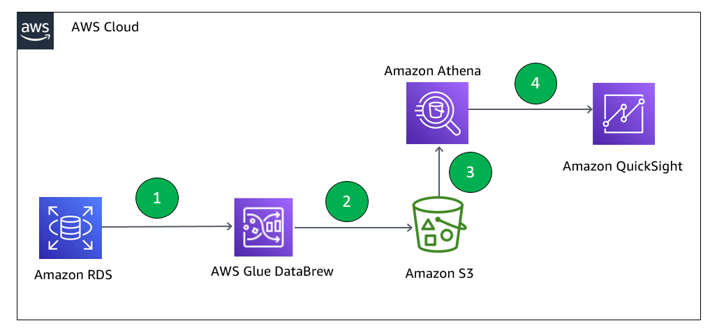
To demonstrate using EXPLAIN and EXPLAIN ANALYZE statements, we use the following services and resources:

• Five database tables from the Major League Baseball dataset
• AWS CloudFormation to provision AWS resources
• Amazon S3, Amazon DynamoDB, and Amazon Aurora MySQL-Compatible Edition as data storage

Athena uses the AWS Glue Data Catalog to store and retrieve table metadata for the Amazon S3 data in your AWS account. The table metadata lets the Athena query engine know how to find, read, and process the data that you want to query. We use Athena data source connectors to connect to data sources external to Amazon S3.

Prerequisites

To deploy the CloudFormation template, you must have the following:

• An AWS account
• An AWS Identity and Access Management (IAM) user with access to the following services:
  • Amazon Athena
  • AWS CloudFormation
  • Amazon DynamoDB
  • AWS Glue
  • AWS Lambda
  • Amazon Relational Database Service (Amazon RDS)
  • Amazon S3
  • Amazon Virtual Private Cloud (Amazon VPC)

Provision resources with AWS CloudFormation

To deploy the CloudFormation template, complete the following steps:

1. Choose Launch Stack:

2. Follow the prompts on the AWS CloudFormation console to create the stack.
3. Note the key-value pairs on the stack’s Outputs tab.

You use these values when configuring the Athena data source connectors.

The CloudFormation template creates the following resources:

• S3 buckets to store data and act as temporary spill buckets for Lambda
• AWS Glue Data Catalog tables for the data in the S3 buckets
• A DynamoDB table and Amazon RDS for MySQL tables, which are used to join multiple tables from different sources
• A VPC, subnets, and endpoints, which are needed for Amazon RDS for MySQL and DynamoDB

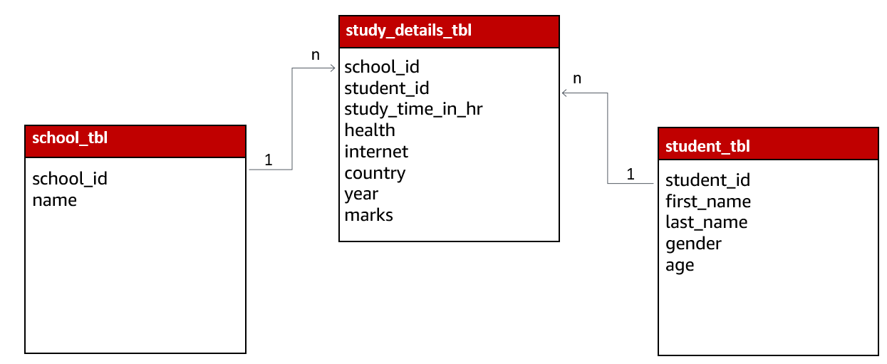
The following figure shows the high-level data model for the data load.

Create the DynamoDB data source connector

To create the DynamoDB connector for Athena, complete the following steps:

1. On the Athena console, choose Data sources in the navigation pane.
2. Choose Create data source.
3. For Data sources, select Amazon DynamoDB.
4. Choose Next.

5. For Data source name, enter DDB.

6. For Lambda function, choose Create Lambda function.

This opens a new tab in your browser.

7. For Application name, enter AthenaDynamoDBConnector.
8. For SpillBucket, enter the value from the CloudFormation stack for AthenaSpillBucket.
9. For AthenaCatalogName, enter dynamodb-lambda-func.
10. Leave the remaining values at their defaults.
11. Select I acknowledge that this app creates custom IAM roles and resource policies.
12. Choose Deploy.

You’re returned to the Connect data sources section on the Athena console.

13. Choose the refresh icon next to Lambda function.
14. Choose the Lambda function you just created (dynamodb-lambda-func).

15. Choose Next.
16. Review the settings and choose Create data source.
17. If you haven’t already set up the Athena query results location, choose View settings on the Athena query editor page.

18. Choose Manage.
19. For Location of query result, browse to the S3 bucket specified for the Athena spill bucket in the CloudFormation template.
20. Add Athena-query to the S3 path.
21. Choose Save.

22. In the Athena query editor, for Data source, choose DDB.
23. For Database, choose default.

You can now explore the schema for the sportseventinfo table; the data is the same in DynamoDB.

24. Choose the options icon for the sportseventinfo table and choose Preview Table.

Create the Amazon RDS for MySQL data source connector

Now let’s create the connector for Amazon RDS for MySQL.

1. On the Athena console, choose Data sources in the navigation pane.
2. Choose Create data source.
3. For Data sources, select MySQL.
4. Choose Next.

5. For Data source name, enter MySQL.

6. For Lambda function, choose Create Lambda function.

7. For Application name, enter AthenaMySQLConnector.
8. For SecretNamePrefix, enter AthenaMySQLFederation.
9. For SpillBucket, enter the value from the CloudFormation stack for AthenaSpillBucket.
10. For DefaultConnectionString, enter the value from the CloudFormation stack for MySQLConnection.
11. For LambdaFunctionName, enter mysql-lambda-func.
12. For SecurityGroupIds, enter the value from the CloudFormation stack for RDSSecurityGroup.
13. For SubnetIds, enter the value from the CloudFormation stack for RDSSubnets.
14. Select I acknowledge that this app creates custom IAM roles and resource policies.
15. Choose Deploy.

16. On the Lambda console, open the function you created (mysql-lambda-func).
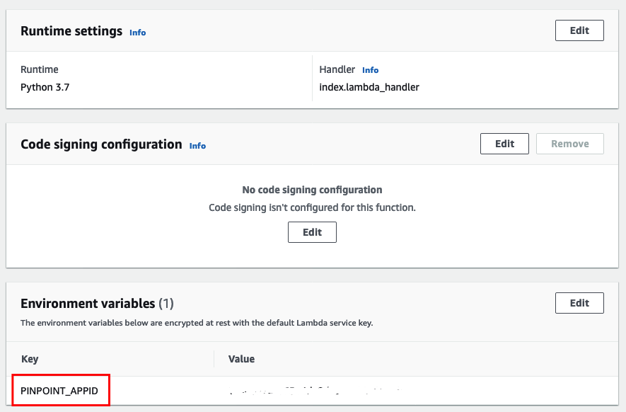
17. On the Configuration tab, under Environment variables, choose Edit.

18. Choose Add environment variable.
19. Enter a new key-value pair:
    • For Key, enter MYSQL_connection_string.
    • For Value, enter the value from the CloudFormation stack for MySQLConnection.
20. Choose Save.

21. Return to the Connect data sources section on the Athena console.
22. Choose the refresh icon next to Lambda function.
23. Choose the Lambda function you created (mysql-lamdba-function).

24. Choose Next.
25. Review the settings and choose Create data source.
26. In the Athena query editor, for Data Source, choose MYSQL.
27. For Database, choose sportsdata.

28. Choose the options icon by the tables and choose Preview Table to examine the data and schema.

In the following sections, we demonstrate different ways to optimize our queries.

Optimal join order using EXPLAIN plan

A join is a basic SQL operation to query data on multiple tables using relations on matching columns. Join operations affect how much data is read from a table, how much data is transferred to the intermediate stages through networks, and how much memory is needed to build up a hash table to facilitate a join.

If you have multiple join operations and these join tables aren’t in the correct order, you may experience performance issues. To demonstrate this, we use the following tables from difference sources and join them in a certain order. Then we observe the query runtime and improve performance by using the EXPLAIN feature from Athena, which provides some suggestions for optimizing the query.

The CloudFormation template you ran earlier loaded data into the following services:

Let’s construct a query to find all those who participated in the event by type of tickets. The query runtime with the following join took approximately 7 mins to complete:

SELECT t.id AS ticket_id, 
e.eventid, 
p.first_name 
FROM 
"DDB"."default"."sportseventinfo" e, 
"AwsDataCatalog"."athenablog"."person" p, 
"AwsDataCatalog"."athenablog"."ticketinfo" t 
WHERE 
t.sporting_event_id = cast(e.eventid as double) 
AND t.ticketholder_id = p.id

Now let’s use EXPLAIN on the query to see its run plan. We use the same query as before, but add explain (TYPE DISTRIBUTED):

EXPLAIN (TYPE DISTRIBUTED)
SELECT t.id AS ticket_id, 
e.eventid, 
p.first_name 
FROM 
"DDB"."default"."sportseventinfo" e, 
"AwsDataCatalog"."athenablog"."person" p, 
"AwsDataCatalog"."athenablog"."ticketinfo" t 
WHERE 
t.sporting_event_id = cast(e.eventid as double) 
AND t.ticketholder_id = p.id

The following screenshot shows our output

Notice the cross-join in Fragment 1. The joins are converted to a Cartesian product for each table, where every record in a table is compared to every record in another table. Therefore, this query takes a significant amount of time to complete.

To optimize our query, we can rewrite it by reordering the joining tables as sportseventinfo first, ticketinfo second, and person last. The reason for this is because the WHERE clause, which is being converted to a JOIN ON clause during the query plan stage, doesn’t have the join relationship between the person table and sportseventinfo table. Therefore, the query plan generator converted the join type to cross-joins (a Cartesian product), which less efficient. Reordering the tables aligns the WHERE clause to the INNER JOIN type, which satisfies the JOIN ON clause and runtime is reduced from 7 minutes to 10 seconds.

The code for our optimized query is as follows:

SELECT t.id AS ticket_id, 
e.eventid, 
p.first_name 
FROM 
"DDB"."default"."sportseventinfo" e, 
"AwsDataCatalog"."athenablog"."ticketinfo" t, 
"AwsDataCatalog"."athenablog"."person" p 
WHERE 
t.sporting_event_id = cast(e.eventid as double) 
AND t.ticketholder_id = p.id

The following is the EXPLAIN output of our query after reordering the join clause:

EXPLAIN (TYPE DISTRIBUTED) 
SELECT t.id AS ticket_id, 
e.eventid, 
p.first_name 
FROM 
"DDB"."default"."sportseventinfo" e, 
"AwsDataCatalog"."athenablog"."ticketinfo" t, 
"AwsDataCatalog"."athenablog"."person" p 
WHERE t.sporting_event_id = cast(e.eventid as double) 
AND t.ticketholder_id = p.id

The following screenshot shows our output.

The cross-join changed to INNER JOIN with join on columns (eventid, id, ticketholder_id), which results in the query running faster. Joins between the ticketinfo and person tables converted to the PARTITION distribution type, where both left and right tables are hash-partitioned across all worker nodes due to the size of the person table. The join between the sportseventinfo table and ticketinfo are converted to the REPLICATED distribution type, where one table is hash-partitioned across all worker nodes and the other table is replicated to all worker nodes to perform the join operation.

For more information about how to analyze these results, refer to Understanding Athena EXPLAIN statement results.

As a best practice, we recommend having a JOIN statement along with an ON clause, as shown in the following code:

SELECT t.id AS ticket_id, 
e.eventid, 
p.first_name 
FROM 
"AwsDataCatalog"."athenablog"."person" p 
JOIN "AwsDataCatalog"."athenablog"."ticketinfo" t ON t.ticketholder_id = p.id 
JOIN "ddb"."default"."sportseventinfo" e ON t.sporting_event_id = cast(e.eventid as double)

Also as a best practice when you join two tables, specify the larger table on the left side of join and the smaller table on the right side of the join. Athena distributes the table on the right to worker nodes, and then streams the table on the left to do the join. If the table on the right is smaller, then less memory is used and the query runs faster.

In the following sections, we present examples of how to optimize pushdowns for filter predicates and projection filter operations for the Athena data source using EXPLAIN ANALYZE.

Pushdown optimization for the Athena connector for Amazon RDS for MySQL

A pushdown is an optimization to improve the performance of a SQL query by moving its processing as close to the data as possible. Pushdowns can drastically reduce SQL statement processing time by filtering data before transferring it over the network and filtering data before loading it into memory. The Athena connector for Amazon RDS for MySQL supports pushdowns for filter predicates and projection pushdowns.

The following table summarizes the services and tables we use to demonstrate a pushdown using Aurora MySQL.

We use the following query as an example of a filtering predicate and projection filter:

SELECT full_name,
name 
FROM "sportsdata"."player_partitioned" a 
JOIN "sportsdata"."sport_team_partitioned" b ON a.sport_team_id=b.id 
WHERE a.id='1.0'

This query selects the players and their team based on their ID. It serves as an example of both filter operations in the WHERE clause and projection because it selects only two columns.

We use EXPLAIN ANALYZE to get the cost for the running this query:

EXPLAIN ANALYZE 
SELECT full_name,
name 
FROM "MYSQL"."sportsdata"."player_partitioned" a 
JOIN "MYSQL"."sportsdata"."sport_team_partitioned" b ON a.sport_team_id=b.id 
WHERE a.id='1.0'

The following screenshot shows the output in Fragment 2 for the table player_partitioned, in which we observe that the connector has a successful pushdown filter on the source side, so it tries to scan only one record out of the 5,157 records in the table. The output also shows that the query scan has only two columns (full_name as the projection column and sport_team_id and the join column), and uses SELECT and JOIN, which indicates the projection pushdown is successful. This helps reduce the data scan when using Athena data source connectors.

Now let’s look at the conditions in which a filter predicate pushdown doesn’t work with Athena connectors.

LIKE statement in filter predicates

We start with the following example query to demonstrate using the LIKE statement in filter predicates:

SELECT * 
FROM "MYSQL"."sportsdata"."player_partitioned" 
WHERE first_name LIKE '%Aar%'

We then add EXPLAIN ANALYZE:

EXPLAIN ANALYZE 
SELECT * 
FROM "MYSQL"."sportsdata"."player_partitioned" 
WHERE first_name LIKE '%Aar%'

The EXPLAIN ANALYZE output shows that the query performs the table scan (scanning the table player_partitioned, which contains 5,157 records) for all the records even though the WHERE clause only has 30 records matching the condition %Aar%. Therefore, the data scan shows the complete table size even with the WHERE clause.

We can optimize the same query by selecting only the required columns:

EXPLAIN ANALYZE 
SELECT sport_team_id,
full_name 
FROM "MYSQL"."sportsdata"."player_partitioned" 
WHERE first_name LIKE '%Aar%'

From the EXPLAIN ANALYZE output, we can observe that the connector supports the projection filter pushdown, because we select only two columns. This brought the data scan size down to half of the table size.

OR statement in filter predicates

We start with the following query to demonstrate using the OR statement in filter predicates:

SELECT id,
first_name 
FROM "MYSQL"."sportsdata"."player_partitioned" 
WHERE first_name = 'Aaron' OR id ='1.0'

We use EXPLAIN ANALYZE with the preceding query as follows:

EXPLAIN ANALYZE 
SELECT * 
FROM 
"MYSQL"."sportsdata"."player_partitioned" 
WHERE first_name = 'Aaron' OR id ='1.0'

Similar to the LIKE statement, the following output shows that query scanned the table instead of pushing down to only the records that matched the WHERE clause. This query outputs only 16 records, but the data scan indicates a complete scan.

Pushdown optimization for the Athena connector for DynamoDB

For our example using the DynamoDB connector, we use the following data:

Let’s test the filter predicate and project filter operation for our DynamoDB table using the following query. This query tries to get all the events and sports for a given location. We use EXPLAIN ANALYZE for the query as follows:

EXPLAIN ANALYZE 
SELECT EventId,
Sport 
FROM "DDB"."default"."sportseventinfo" 
WHERE Location = 'Chase Field'

The output of EXPLAIN ANALYZE shows that the filter predicate retrieved only 21 records, and the project filter selected only two columns to push down to the source. Therefore, the data scan for this query is less than the table size.

Now let’s see where filter predicate pushdown doesn’t work. In the WHERE clause, if you apply the TRIM() function to the Location column and then filter, predicate pushdown optimization doesn’t apply, but we still see the projection filter optimization, which does apply. See the following code:

EXPLAIN ANALYZE 
SELECT EventId,
Sport 
FROM "DDB"."default"."sportseventinfo" 
WHERE trim(Location) = 'Chase Field'

The output of EXPLAIN ANALYZE for this query shows that the query scans all the rows but is still limited to only two columns, which shows that the filter predicate doesn’t work when the TRIM function is applied.

We’ve seen from the preceding examples that the Athena data source connector for Amazon RDS for MySQL and DynamoDB do support filter predicates and projection predicates for pushdown optimization, but we also saw that operations such as LIKE, OR, and TRIM when used in the filter predicate don’t support pushdowns to the source. Therefore, if you encounter unexplained charges in your federated Athena query, we recommend using EXPLAIN ANALYZE with the query and determine whether your Athena connector supports the pushdown operation or not.

Please note that running EXPLAIN ANALYZE incurs cost because it scans the data.

Conclusion

In this post, we showcased how to use EXPLAIN and EXPLAIN ANALYZE to analyze Athena SQL queries for data sources on AWS S3 and Athena federated SQL query for data source like DynamoDB and Amazon RDS for MySQL. You can use this as an example to optimize queries which would also result in cost savings.

About the Authors

Nishchai JM is an Analytics Specialist Solutions Architect at Amazon Web services. He specializes in building Big-data applications and help customer to modernize their applications on Cloud. He thinks Data is new oil and spends most of his time in deriving insights out of the Data.

Varad Ram is Senior Solutions Architect in Amazon Web Services. He likes to help customers adopt to cloud technologies and is particularly interested in artificial intelligence. He believes deep learning will power future technology growth. In his spare time, he like to be outdoor with his daughter and son.