All posts by Florian Mair

Krones real-time production line monitoring with Amazon Managed Service for Apache Flink

Post Syndicated from Florian Mair original https://aws.amazon.com/blogs/big-data/krones-real-time-production-line-monitoring-with-amazon-managed-service-for-apache-flink/

Krones provides breweries, beverage bottlers, and food producers all over the world with individual machines and complete production lines. Every day, millions of glass bottles, cans, and PET containers run through a Krones line. Production lines are complex systems with lots of possible errors that could stall the line and decrease the production yield. Krones wants to detect the failure as early as possible (sometimes even before it happens) and notify production line operators to increase reliability and output. So how to detect a failure? Krones equips their lines with sensors for data collection, which can then be evaluated against rules. Krones, as the line manufacturer, as well as the line operator have the possibility to create monitoring rules for machines. Therefore, beverage bottlers and other operators can define their own margin of error for the line. In the past, Krones used a system based on a time series database. The main challenges were that this system was hard to debug and also queries represented the current state of machines but not the state transitions.

This post shows how Krones built a streaming solution to monitor their lines, based on Amazon Kinesis and Amazon Managed Service for Apache Flink. These fully managed services reduce the complexity of building streaming applications with Apache Flink. Managed Service for Apache Flink manages the underlying Apache Flink components that provide durable application state, metrics, logs, and more, and Kinesis enables you to cost-effectively process streaming data at any scale. If you want to get started with your own Apache Flink application, check out the GitHub repository for samples using the Java, Python, or SQL APIs of Flink.

Overview of solution

Krones’s line monitoring is part of the Krones Shopfloor Guidance system. It provides support in the organization, prioritization, management, and documentation of all activities in the company. It allows them to notify an operator if the machine is stopped or materials are required, regardless where the operator is in the line. Proven condition monitoring rules are already built-in but can also be user defined via the user interface. For example, if a certain data point that is monitored violates a threshold, there can be a text message or trigger for a maintenance order on the line.

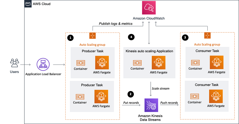
The condition monitoring and rule evaluation system is built on AWS, using AWS analytics services. The following diagram illustrates the architecture.

Architecture Diagram for Krones Production Line Monitoring

Almost every data streaming application consists of five layers: data source, stream ingestion, stream storage, stream processing, and one or more destinations. In the following sections, we dive deeper into each layer and how the line monitoring solution, built by Krones, works in detail.

Data source

The data is gathered by a service running on an edge device reading several protocols like Siemens S7 or OPC/UA. Raw data is preprocessed to create a unified JSON structure, which makes it easier to process later on in the rule engine. A sample payload converted to JSON might look like the following:

{
  "version": 1,
  "timestamp": 1234,
  "equipmentId": "84068f2f-3f39-4b9c-a995-d2a84d878689",
  "tag": "water_temperature",
  "value": 13.45,
  "quality": "Ok",
  "meta": {      
    "sequenceNumber": 123,
    "flags": ["Fst", "Lst", "Wmk", "Syn", "Ats"],
    "createdAt": 12345690,
    "sourceId": "filling_machine"
  }
}

Stream ingestion

AWS IoT Greengrass is an open source Internet of Things (IoT) edge runtime and cloud service. This allows you to act on data locally and aggregate and filter device data. AWS IoT Greengrass provides prebuilt components that can be deployed to the edge. The production line solution uses the stream manager component, which can process data and transfer it to AWS destinations such as AWS IoT Analytics, Amazon Simple Storage Service (Amazon S3), and Kinesis. The stream manager buffers and aggregates records, then sends it to a Kinesis data stream.

Stream storage

The job of the stream storage is to buffer messages in a fault tolerant way and make it available for consumption to one or more consumer applications. To achieve this on AWS, the most common technologies are Kinesis and Amazon Managed Streaming for Apache Kafka (Amazon MSK). For storing our sensor data from production lines, Krones choose Kinesis. Kinesis is a serverless streaming data service that works at any scale with low latency. Shards within a Kinesis data stream are a uniquely identified sequence of data records, where a stream is composed of one or more shards. Each shard has 2 MB/s of read capacity and 1 MB/s write capacity (with max 1,000 records/s). To avoid hitting those limits, data should be distributed among shards as evenly as possible. Every record that is sent to Kinesis has a partition key, which is used to group data into a shard. Therefore, you want to have a large number of partition keys to distribute the load evenly. The stream manager running on AWS IoT Greengrass supports random partition key assignments, which means that all records end up in a random shard and the load is distributed evenly. A disadvantage of random partition key assignments is that records aren’t stored in order in Kinesis. We explain how to solve this in the next section, where we talk about watermarks.

Watermarks

A watermark is a mechanism used to track and measure the progress of event time in a data stream. The event time is the timestamp from when the event was created at the source. The watermark indicates the timely progress of the stream processing application, so all events with an earlier or equal timestamp are considered as processed. This information is essential for Flink to advance event time and trigger relevant computations, such as window evaluations. The allowed lag between event time and watermark can be configured to determine how long to wait for late data before considering a window complete and advancing the watermark.

Krones has systems all around the globe, and needed to handle late arrivals due to connection losses or other network constraints. They started out by monitoring late arrivals and setting the default Flink late handling to the maximum value they saw in this metric. They experienced issues with time synchronization from the edge devices, which lead them to a more sophisticated way of watermarking. They built a global watermark for all the senders and used the lowest value as the watermark. The timestamps are stored in a HashMap for all incoming events. When the watermarks are emitted periodically, the smallest value of this HashMap is used. To avoid stalling of watermarks by missing data, they configured an idleTimeOut parameter, which ignores timestamps that are older than a certain threshold. This increases latency but gives strong data consistency.

public class BucketWatermarkGenerator implements WatermarkGenerator<DataPointEvent> {
private HashMap <String, WatermarkAndTimestamp> lastTimestamps;
private Long idleTimeOut;
private long maxOutOfOrderness;
}

Stream processing

After the data is collected from sensors and ingested into Kinesis, it needs to be evaluated by a rule engine. A rule in this system represents the state of a single metric (such as temperature) or a collection of metrics. To interpret a metric, more than one data point is used, which is a stateful calculation. In this section, we dive deeper into the keyed state and broadcast state in Apache Flink and how they’re used to build the Krones rule engine.

Control stream and broadcast state pattern

In Apache Flink, state refers to the ability of the system to store and manage information persistently across time and operations, enabling the processing of streaming data with support for stateful computations.

The broadcast state pattern allows the distribution of a state to all parallel instances of an operator. Therefore, all operators have the same state and data can be processed using this same state. This read-only data can be ingested by using a control stream. A control stream is a regular data stream, but usually with a much lower data rate. This pattern allows you to dynamically update the state on all operators, enabling the user to change the state and behavior of the application without the need for a redeploy. More precisely, the distribution of the state is done by the use of a control stream. By adding a new record into the control stream, all operators receive this update and are using the new state for the processing of new messages.

This allows users of Krones application to ingest new rules into the Flink application without restarting it. This avoids downtime and gives a great user experience as changes happen in real time. A rule covers a scenario in order to detect a process deviation. Sometimes, the machine data is not as easy to interpret as it might look at first glance. If a temperature sensor is sending high values, this might indicate an error, but also be the effect of an ongoing maintenance procedure. It’s important to put metrics in context and filter some values. This is achieved by a concept called grouping.

Grouping of metrics

The grouping of data and metrics allows you to define the relevance of incoming data and produce accurate results. Let’s walk through the example in the following figure.

Grouping of metrics

In Step 1, we define two condition groups. Group 1 collects the machine state and which product is going through the line. Group 2 uses the value of the temperature and pressure sensors. A condition group can have different states depending on the values it receives. In this example, group 1 receives data that the machine is running, and the one-liter bottle is selected as the product; this gives this group the state ACTIVE. Group 2 has metrics for temperature and pressure; both metrics are above their thresholds for more than 5 minutes. This results in group 2 being in a WARNING state. This means group 1 reports that everything is fine and group 2 does not. In Step 2, weights are added to the groups. This is needed in some situations, because groups might report conflicting information. In this scenario, group 1 reports ACTIVE and group 2 reports WARNING, so it’s not clear to the system what the state of the line is. After adding the weights, the states can be ranked, as shown in step 3. Lastly, the highest ranked state is chosen as the winning one, as shown in Step 4.

After the rules are evaluated and the final machine state is defined, the results will be further processed. The action taken depends on the rule configuration; this can be a notification to the line operator to restock materials, do some maintenance, or just a visual update on the dashboard. This part of the system, which evaluates metrics and rules and takes actions based on the results, is referred to as a rule engine.

Scaling the rule engine

By letting users build their own rules, the rule engine can have a high number of rules that it needs to evaluate, and some rules might use the same sensor data as other rules. Flink is a distributed system that scales very well horizontally. To distribute a data stream to several tasks, you can use the keyBy() method. This allows you to partition a data stream in a logical way and send parts of the data to different task managers. This is often done by choosing an arbitrary key so you get an evenly distributed load. In this case, Krones added a ruleId to the data point and used it as a key. Otherwise, data points that are needed are processed by another task. The keyed data stream can be used across all rules just like a regular variable.
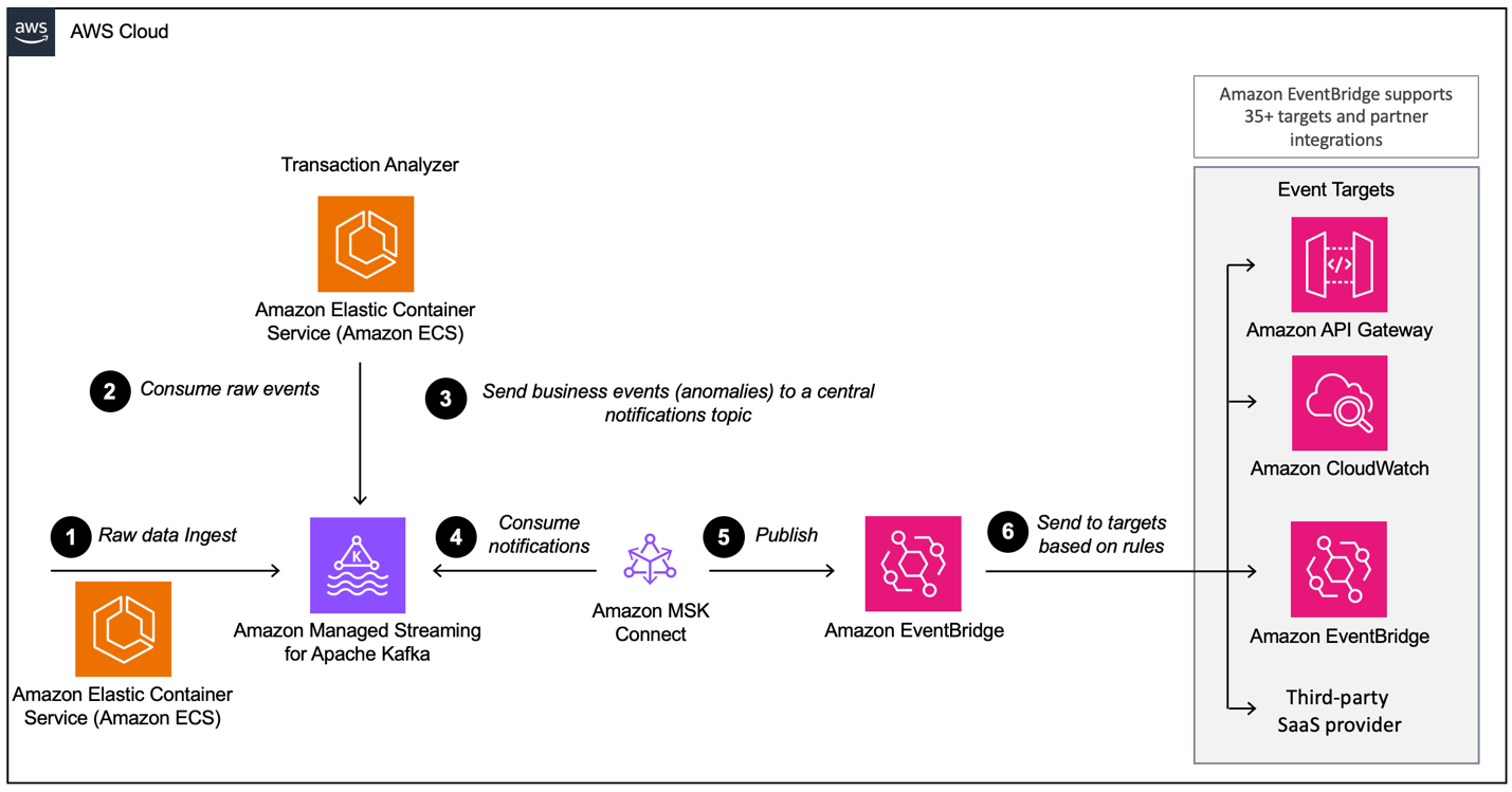
Destinations

When a rule changes its state, the information is sent to a Kinesis stream and then via Amazon EventBridge to consumers. One of the consumers creates a notification from the event that is transmitted to the production line and alerts the personnel to act. To be able to analyze the rule state changes, another service writes the data to an Amazon DynamoDB table for fast access and a TTL is in place to offload long-term history to Amazon S3 for further reporting.

Conclusion

In this post, we showed you how Krones built a real-time production line monitoring system on AWS. Managed Service for Apache Flink allowed the Krones team to get started quickly by focusing on application development rather than infrastructure. The real-time capabilities of Flink enabled Krones to reduce machine downtime by 10% and increase efficiency up to 5%.

If you want to build your own streaming applications, check out the available samples on the GitHub repository. If you want to extend your Flink application with custom connectors, see Making it Easier to Build Connectors with Apache Flink: Introducing the Async Sink. The Async Sink is available in Apache Flink version 1.15.1 and later.


About the Authors

Florian Mair is a Senior Solutions Architect and data streaming expert at AWS. He is a technologist that helps customers in Europe succeed and innovate by solving business challenges using AWS Cloud services. Besides working as a Solutions Architect, Florian is a passionate mountaineer, and has climbed some of the highest mountains across Europe.

Emil Dietl is a Senior Tech Lead at Krones specializing in data engineering, with a key field in Apache Flink and microservices. His work often involves the development and maintenance of mission-critical software. Outside of his professional life, he deeply values spending quality time with his family.

Simon Peyer is a Solutions Architect at AWS based in Switzerland. He is a practical doer and is passionate about connecting technology and people using AWS Cloud services. A special focus for him is data streaming and automations. Besides work, Simon enjoys his family, the outdoors, and hiking in the mountains.

Build event-driven architectures with Amazon MSK and Amazon EventBridge

Post Syndicated from Florian Mair original https://aws.amazon.com/blogs/big-data/build-event-driven-architectures-with-amazon-msk-and-amazon-eventbridge/

Based on immutable facts (events), event-driven architectures (EDAs) allow businesses to gain deeper insights into their customers’ behavior, unlocking more accurate and faster decision-making processes that lead to better customer experiences. In EDAs, modern event brokers, such as Amazon EventBridge and Apache Kafka, play a key role to publish and subscribe to events. EventBridge is a serverless event bus that ingests data from your own apps, software as a service (SaaS) apps, and AWS services and routes that data to targets. Although there is overlap in their role as the backbone in EDAs, both solutions emerged from different problem statements and provide unique features to solve specific use cases. With a solid understanding of both technologies and their primary use cases, developers can create easy-to-use, maintainable, and evolvable EDAs.

If the use case is well defined and directly maps to one event bus, such as event streaming and analytics with streaming events (Kafka) or application integration with simplified and consistent event filtering, transformation, and routing on discrete events (EventBridge), the decision for a particular broker technology is straightforward. However, organizations and business requirements are often more complex and beyond the capabilities of one broker technology. In almost any case, choosing an event broker should not be a binary decision. Combining complementary broker technologies and embracing their unique strengths is a solid approach to build easy-to-use, maintainable, and evolvable EDAs. To make the integration between Kafka and EventBridge even smoother, AWS open-sourced the EventBridge Connector based on Apache Kafka. This allows you to consume from on-premises Kafka deployments and avoid point-to-point communication, while using the existing knowledge and toolset of Kafka Connect.

Streaming applications enable stateful computations over unbound datasets. This allows real-time use cases such as anomaly detection, event-time computations, and much more. These applications can be built using frameworks such as Apache Flink, Apache Spark, or Kafka Streams. Although some of those frameworks support sending events to downstream systems other than Apache Kafka, there is no standardized way of doing so across frameworks. It would require each application owner to build their own logic to send events downstream. In an EDA, the preferred way to handle such a scenario is to publish events to an event bus and then send them downstream.

There are two ways to send events from Apache Kafka to EventBridge: the preferred method using Amazon EventBridge Pipes or the EventBridge sink connector for Kafka Connect. In this post, we explore when to use which option and how to build an EDA using the EventBridge sink connector and Amazon Managed Streaming for Apache Kafka (Amazon MSK).

EventBridge sink connector vs. EventBridge Pipes

EventBridge Pipes connects sources to targets with a point-to-point integration, supporting event filtering, transformations, enrichment, and event delivery to over 14 AWS services and external HTTPS-based targets using API Destinations. This is the preferred and most easy method to send events from Kafka to EventBridge as it simplifies the setup and operations with a delightful developer experience.

Alternatively, under the following circumstances you might want to choose the EventBridge sink connector to send events from Kafka directly to EventBridge Event Buses:

  • You are have already invested in processes and tooling around the Kafka Connect framework as the platform of your choice to integrate with other systems and services
  • You need to integrate with a Kafka-compatible schema registry e.g., the AWS Glue Schema Registry, supporting Avro and Protobuf data formats for event serialization and deserialization
  • You want to send events from on-premises Kafka environments directly to EventBridge Event Buses

Overview of solution

In this post, we show you how to use Kafka Connect and the EventBridge sink connector to send Avro-serialized events from Amazon Managed Streaming for Apache Kafka (Amazon MSK) to EventBridge. This enables a seamless and consistent data flow from Apache Kafka to dozens of supported EventBridge AWS and partner targets, such as Amazon CloudWatch, Amazon SQS, AWS Lambda, and HTTPS targets like Salesforce, Datadog, and Snowflake using EventBridge API destinations. The following diagram illustrates the event-driven architecture used in this blog post based on Amazon MSK and EventBridge.

Architecture Diagram

The workflow consists of the following steps:

  1. The demo application generates credit card transactions, which are sent to Amazon MSK using the Avro format.
  2. An analytics application running on Amazon Elastic Container Service (Amazon ECS) consumes the transactions and analyzes them if there is an anomaly.
  3. If an anomaly is detected, the application emits a fraud detection event back to the MSK notification topic.
  4. The EventBridge connector consumes the fraud detection events from Amazon MSK in Avro format.
  5. The connector converts the events to JSON and sends them to EventBridge.
  6. In EventBridge, we use JSON filtering rules to filter our events and send them to other services or another Event Bus. In this example, fraud detection events are sent to Amazon CloudWatch Logs for auditing and introspection, and to a third-party SaaS provider to showcase how easy it is to integrate with third-party APIs, such as Salesforce.

Prerequisites

For this walkthrough, you should have the following prerequisites:

Deploy the AWS CDK stack

This walkthrough requires you to deploy an AWS CDK stack to your account. You can deploy the full stack end to end or just the required resources to follow along with this post.

  1. In your terminal, run the following command:
    git clone https://github.com/awslabs/eventbridge-kafka-connector/

  2. Navigate to the cdk directory:
    cd eventbridge-kafka-connector/cdk

  3. Deploy the AWS CDK stack based on your preferences:
  4. If you want to see the complete setup explained in this post, run the following command:
    cdk deploy —context deployment=FULL

  5. If you want to deploy the connector on your own but have the required resources already, including the MSK cluster, AWS Identity and Access Management (IAM) roles, security groups, data generator, and so on, run the following command:
    cdk deploy —context deployment=PREREQ

Deploy the EventBridge sink connector on Amazon MSK Connect

If you deployed the CDK stack in FULL mode, you can skip this section and move on to Create EventBridge rules.

The connector needs an IAM role that allows reading the data from the MSK cluster and sending records downstream to EventBridge.

Upload connector code to Amazon S3

Complete the following steps to upload the connector code to Amazon Simple Storage Service (Amazon S3):

  1. Navigate to the GitHub repo.
  2. Download the release 1.0.0 with the AWS Glue Schema Registry dependencies included.
  3. On the Amazon S3 console, choose Buckets in the navigation pane.
  4. Choose Create bucket.
  5. For Bucket name, enter eventbridgeconnector-bucket-${AWS_ACCOUNT_ID}.

As Because S3 buckets must be globally unique, replace ${AWS_ACCOUNT_ID} with your actual AWS account ID. For example, eventbridgeconnector-bucket-123456789012.

  1. Open the bucket and choose Upload.
  2. Select the .jar file that you downloaded from the GitHub repository and choose Upload.

S3 File Upload Console

Create a custom plugin

We now have our application code in Amazon S3. As a next step, we create a custom plugin in Amazon MSK Connect. Complete the following steps:

  1. On the Amazon MSK console, choose Custom plugins in the navigation pane under MSK Connect.
  2. Choose Create custom plugin.
  3. For S3 URI – Custom plugin object, browse to the file named kafka-eventbridge-sink-with-gsr-dependencies.jar in the S3 bucket eventbridgeconnector-bucket-${AWS_ACCOUNT_ID} for the EventBridge connector.
  4. For Custom plugin name, enter msk-eventBridge-sink-plugin-v1.
  5. Enter an optional description.
  6. Choose Create custom plugin.

MSK Connect Plugin Screen

  1. Wait for plugin to transition to the status Active.

Create a connector

Complete the following steps to create a connector in MSK Connect:

  1. On the Amazon MSK console, choose Connectors in the navigation pane under MSK Connect.
  2. Choose Create connector.
  3. Select Use existing custom plugin and under Custom plugins, select the plugin msk-eventBridge-sink-plugin-v1 that you created earlier.
  4. Choose Next.
  5. For Connector name, enter msk-eventBridge-sink-connector.
  6. Enter an optional description.
  7. For Cluster type, select MSK cluster.
  8. For MSK clusters, select the cluster you created earlier.
  9. For Authentication, choose IAM.
  10. Under Connector configurations, enter the following settings (for more details on the configuration, see the GitHub repository):
    auto.offset.reset=earliest
    connector.class=software.amazon.event.kafkaconnector.EventBridgeSinkConnector
    topics=notifications
    aws.eventbridge.connector.id=avro-test-connector
    aws.eventbridge.eventbus.arn=arn:aws:events:us-east-1:123456789012:event-bus/eventbridge-sink-eventbus
    aws.eventbridge.region=us-east-1
    tasks.max=1
    key.converter=org.apache.kafka.connect.storage.StringConverter
    value.converter=com.amazonaws.services.schemaregistry.kafkaconnect.AWSKafkaAvroConverter
    value.converter.region=us-east-1
    value.converter.registry.name=default-registry
    value.converter.avroRecordType=GENERIC_RECORD

  11. Make sure to replace aws.eventbridge.eventbus.arn, aws.eventbridge.region, and value.converter.region with the values from the prerequisite stack.
  12. In the Connector capacity section, select Autoscaled for Capacity type.
  13. Leave the default value of 1 for MCU count per worker.
  14. Keep all default values for Connector capacity.
  15. For Worker configuration, select Use the MSK default configuration.
  16. Under Access permissions, choose the custom IAM role KafkaEventBridgeSinkStack-connectorRole, which you created during the AWS CDK stack deployment.
  17. Choose Next.
  18. Choose Next again.
  19. For Log delivery, select Deliver to Amazon CloudWatch Logs.
  20. For Log group, choose /aws/mskconnect/eventBridgeSinkConnector.
  21. Choose Next.
  22. Under Review and Create, validate all the settings and choose Create connector.

The connector will be now in the state Creating. It can take up to several minutes for the connector to transition into the status Running.

Create EventBridge rules

Now that the connector is forwarding events to EventBridge, we can use EventBridge rules to filter and send events to other targets. Complete the following steps to create a rule:

  1. On the EventBridge console, choose Rules in the navigation pane.
  2. Choose Create rule.
  3. Enter eb-to-cloudwatch-logs-and-webhook for Name.
  4. Select eventbridge-sink-eventbus for Event bus.
  5. Choose Next.
  6. Select Custom pattern (JSON editor), choose Insert, and replace the event pattern with the following code:
    {
      "detail": {
        "value": {
          "eventType": ["suspiciousActivity"],
          "source": ["transactionAnalyzer"]
        }
      },
      "detail-type": [{
        "prefix": "kafka-connect-notification"
      }]
    }
    

  7. Choose Next.
  8. For Target 1, select CloudWatch log group and enter kafka-events for Log Group.
  9. Choose Add another target.
  10. (Optional: Create an API destination) For Target 2, select EventBridge API destination for Target types.
  11. Select Create a new API destination.
  12. Enter a descriptive name for Name.
  13. Add the URL and enter it as API destination endpoint. (This can be the URL of your Datadog, Salesforce, etc. endpoint)
  14. Select POST for HTTP method.
  15. Select Create a new connection for Connection.
  16. For Connection Name, enter a name.
  17. Select Other as Destination type and select API Key as Authorization Type.
  18. For API key name and Value, enter your keys.
  19. Choose Next.
  20. Validate your inputs and choose Create rule.

EventBridge Rule

The following screenshot of the CloudWatch Logs console shows several events from EventBridge.

CloudWatch Logs

Run the connector in production

In this section, we dive deeper into the operational aspects of the connector. Specifically, we discuss how the connector scales and how to monitor it using CloudWatch.

Scale the connector

Kafka connectors scale through the number of tasks. The code design of the EventBridge sink connector doesn’t limit the number of tasks that it can run. MSK Connect provides the compute capacity to run the tasks, which can be from Provisioned or Autoscaled type. During the deployment of the connector, we choose the capacity type Autoscaled and 1 MCU per worker (which represents 1vCPU and 4GiB of memory). This means MSK Connect will scale the infrastructure to run tasks but not the number of tasks. The number of tasks is defined by the connector. By default, the connector will start with the number of tasks defined in tasks.max in the connector configuration. If this value is higher than the partition count of the processed topic, the number of tasks will be set to the number of partitions during the Kafka Connect rebalance.

Monitor the connector

MSK Connect emits metrics to CloudWatch for monitoring by default. Besides MSK Connect metrics, the offset of the connector should also be monitored in production. Monitoring the offset gives insights if the connector can keep up with the data produced in the Kafka cluster.

Clean up

To clean up your resources and avoid ongoing charges, complete the following the steps:

  1. On the Amazon MSK console, choose Connectors in the navigation pane under MSK Connect.
  2. Select the connectors you created and choose Delete.
  3. Choose Clusters in the navigation pane.
  4. Select the cluster you created and choose Delete on the Actions menu.
  5. On the EventBridge console, choose Rules in the navigation pane.
  6. Choose the event bus eventbridge-sink-eventbus.
  7. Select all the rules you created and choose Delete.
  8. Confirm the removal by entering delete, then choose Delete.

If you deployed the AWS CDK stack with the context PREREQ, delete the .jar file for the connector.

  1. On the Amazon S3 console, choose Buckets in the navigation pane.
  2. Navigate to the bucket where you uploaded your connector and delete the kafka-eventbridge-sink-with-gsr-dependencies.jar file.

Independent from the chosen deployment mode, all other AWS resources can be deleted by using AWS CDK or AWS CloudFormation. Run cdk destroy from the repository directory to delete the CloudFormation stack.

Alternatively, on the AWS CloudFormation console, select the stack KafkaEventBridgeSinkStack and choose Delete.

Conclusion

In this post, we showed how you can use MSK Connect to run the AWS open-sourced Kafka connector for EventBridge, how to configure the connector to forward a Kafka topic to EventBridge, and how to use EventBridge rules to filter and forward events to CloudWatch Logs and a webhook.

To learn more about the Kafka connector for EventBridge, refer to Amazon EventBridge announces open-source connector for Kafka Connect, as well as the MSK Connect Developer Guide and the code for the connector on the GitHub repo.


About the Authors

Florian Mair is a Senior Solutions Architect and data streaming expert at AWS. He is a technologist that helps customers in Germany succeed and innovate by solving business challenges using AWS Cloud services. Besides working as a Solutions Architect, Florian is a passionate mountaineer, and has climbed some of the highest mountains across Europe.

Benjamin Meyer is a Senior Solutions Architect at AWS, focused on Games businesses in Germany to solve business challenges by using AWS Cloud services. Benjamin has been an avid technologist for 7 years, and when he’s not helping customers, he can be found developing mobile apps, building electronics, or tending to his cacti.

How Net at Work built an email threat report system on AWS

Post Syndicated from Florian Mair original https://aws.amazon.com/blogs/architecture/how-net-at-work-built-an-email-threat-report-system-on-aws/

Emails are often used as an entry point for malicious software like trojan horses, rootkits, or encryption-based ransomware. The NoSpamProxy offering developed by Net at Work tackles this threat, providing secure and confidential email communication.

A subservice of NoSpamProxy called 32guards is responsible for threat reports of inbound and outbound emails. With the increasing number of NoSpamProxy customers, 32guards was found to have several limitations. 32guards was previously built on a relational database. But with the growth in traffic, this database was not able to keep up with storage demands and expected query performance. Further, the relational database schema was limiting the possibilities of complex pattern detections, due to performance limitations. The NoSpamProxy team decided to rearchitect the service based on the Lake House approach.

The goal was to move away from a one-size-fits-all approach for data analytics and integrate a data lake with purpose-built data stores, unified governance, and smooth data movement.

This post shows how Net at Work modernized their 32guards service, from a relational database to a fully serverless analytics solution. With adoption of the Well-Architected Analytics Lens best practices and the use of fully managed services, the 32guards team was able to build a production-ready application within six weeks.

Architecture for email threat reports and analytics

This section gives a walkthrough of the solution’s architecture, as illustrated in Figure 1.

Figure 1. 32guards threat reports architecture

Figure 1. 32guards threat reports architecture

1. The entry point is an Amazon API Gateway, which receives email metadata in JSON format from the NoSpamProxy fleet. The message contains information about the email in general, email attachments, and URLs in the email. As an example, a subset of the data is presented in JSON as follows:

{
  ...
  "Attachments": [
    {
      "Sha256Hash": "69FB43BD7CCFD79E162B638596402AD1144DD5D762DEC7433111FC88EDD483FE",
      "Classification": 0,
      "Filename": "test.ods.tar.gz",
      "DetectedMimeType": "application/tar+gzip",
      "Size": 5895
    }
  ],
  "Urls": [
    {
      "Url": "http://www.aarhhie.work/",
      "Classification": 0,
    },        {
      "Url": "http://www.netatwork.de/",
      "Classification": 0,
    },
    {
      "Url": "http://aws.amazon.com/",
      "Classification": 0,
    }
  ]
}

2. This JSON message is forwarded to an AWS Lambda function (called “frontend”), which takes care of the further downstream processing. There are two activities the Lambda function initiates:

  • Forwarding the record for real-time analysis/storage
  • Generating a threat report based on the information derived from the data stored in the indicators of compromises (IOCs) Amazon DynamoDB table

IOCs are patterns within the email metadata that are used to determine if emails are safe or not. For example, this could be for a suspicious file attachment or domain.

Threat report for suspicious emails

In the preceding JSON message, the attachments and URLs have been classified with “0” by the email service itself, which indicates that none of them look suspicious. The frontend Lambda function uses the vast number of IOCs stored in the DynamoDB table and heuristics to determine any potential threats within the email. The use of DynamoDB enables fast lookup times to generate a threat report. For the example, the response to the API Gateway in step 2 looks like this:

{
  "ReportedOnUtc": "2021-10-14T14:33:34.5070945Z",
  "Reason": "realtimeSuspiciousOrganisationalDomain",
  "Identifier": "aarhhie.work",
  ...
}

This threat report shows that the top-level domain “aarhiie.work” has been detected as suspicious. The report is used to determine further actions for the email, such as blocking.

Real-time data processing

3. In the real-time analytics flow, the frontend Lambda function ingests email metadata into a data stream using Amazon Kinesis Data Streams. This is a massively scalable, serverless, and durable real-time data streaming service. Compared to a queue, streaming storage permits more than one consumer of the same data.

4. The first consumer is an Apache Flink application running in Amazon Kinesis Data Analytics. This application generates statistical metrics (for example, occurrences of the top-level domain “.work”). The output is stored in Apache Parquet format on Amazon S3. Parquet is a columnar storage format for row-based files like csv.

The second consumer of the streaming data is Amazon Kinesis Data Firehose. Kinesis Data Firehose is a fully managed solution to reliably load streaming data into data lakes, data stores, and analytics services. Within the 32guards service, Kinesis Data Firehose is used to store all email metadata into Amazon S3. The data is stored in Apache Parquet format, which makes queries more time and cost efficient.

IOC detection

Now that we have shown how data is ingested and threat reports are generated to respond quickly to requests, let’s look at how the IOCs are updated. These IOCs are used for generating the threat report within the “frontend” Lambda function. As attack vectors are changing over time, quickly analyzing the data for new threats, is crucial to provide high-quality reports to the NoSpamProxy service.

The incoming email metadata is stored every few minutes in Amazon S3 by Kinesis Data Firehose. To query data directly in Amazon S3, Amazon Athena is used. Athena is a serverless query service that analyzes data stored in Amazon S3, by using standard SQL syntax.

5. To be able to query data in S3, Amazon Athena uses the AWS Glue Data Catalog, which contains the structure of the email metadata stored in the data lake. The data structure is derived from the data itself using AWS Glue Crawlers. Other external downstream processing services like business intelligence applications, also use Amazon Athena to consume the data.

6. Athena queries are initiated on a predefined schedule to update or generate new IOCs. The results of these queries are stored in the DynamoDB table to enable fast lookup times for the “frontend” Lambda.

Conclusion

In this blog post, we showed how Net at Work modernized their 32guards service within their NoSpamProxy product. The previous architecture used a relational database to ingest and store email metadata. This database was running into performance and storage issues, and must be redesigned into a more performant and scalable architecture.

Amazon S3 is used as the storage layer, which can scale up to exabytes of data. With Amazon Athena as the query engine, there is no need to operate a high-performance database cluster, as compute and storage is separated. By using Amazon Kinesis Data Streams and Amazon Kinesis Data Analytics, valuable insight can be generated in real time, and acted upon more quickly.

As a serverless, fully managed solution, the 32guards service has a lower-cost footprint of as much as 50% and requires less maintenance. By moving away from a relational database model, the query runtimes decrease significantly. You can now conduct analyses that have not been feasible before.

Interested in the NoSpamProxy? Read more about NoSpamProxy or sign up for a free trial.

Looking for more architecture content? AWS Architecture Center provides reference architecture diagrams, vetted architecture solutions, Well-Architected best practices, patterns, icons, and more!

Building a scalable streaming data processor with Amazon Kinesis Data Streams on AWS Fargate

Post Syndicated from Florian Mair original https://aws.amazon.com/blogs/big-data/building-a-scalable-streaming-data-processor-with-amazon-kinesis-data-streams-on-aws-fargate/

Data is ubiquitous in businesses today, and the volume and speed of incoming data are constantly increasing. To derive insights from data, it’s essential to deliver it to a data lake or a data store and analyze it. Real-time or near-real-time data delivery can be cost prohibitive, therefore an efficient architecture is key for processing, and becomes more essential with growing data volume and velocity.

In this post, we show you how to build a scalable producer and consumer application for Amazon Kinesis Data Streams running on AWS Fargate. Kinesis Data Streams is a fully managed and scalable data stream that enables you to ingest, buffer, and process data in real time. AWS Fargate is a serverless compute engine for containers that works with AWS container orchestration services like Amazon Elastic Container Service (Amazon ECS), which allows us to easily run, scale, and secure containerized applications.

This solution also uses the Amazon Kinesis Producer Library (KPL) and Amazon Kinesis Client Library (KCL) to ingest data into the stream and to process it. KPL helps you optimize shard utilization in your data stream by specifying settings for aggregation and batching as data is being produced into your data stream. KCL helps you write robust and scalable consumers that can keep up with fluctuating data volumes being sent to your data stream.

The sample code for this post is available in a GitHub repo, which also includes an AWS CloudFormation template to get you started.

What is data streaming?

Before we look into the details of data streaming architectures, let’s get started with a brief overview of data streaming. Streaming data is data that is generated continuously by a large number of sources that transmit the data records simultaneously in small packages. You can use data streaming for many use cases, such as log processing, clickstream analysis, device geo-location, social media data processing, and financial trading.

A data streaming application consists of two layers: the storage layer and the processing layer. As stream storage, AWS offers the managed services Kinesis Data Streams and Amazon Managed Streaming for Apache Kafka (Amazon MSK), but you can also run stream storages like Apache Kafka or Apache Flume on Amazon Elastic Compute Cloud (Amazon EC2) or Amazon EMR. The processing layer consumes the data from the storage layer and runs computations on that data. This could be an Apache Flink application running fully managed on Amazon Kinesis Analytics for Apache Flink, an application running stream processing frameworks like Apache Spark Streaming and Apache Storm or a custom application using the Kinesis API or KCL. For this post, we use Kinesis Data Streams as the storage layer and the containerized KCL application on AWS Fargate as the processing layer.

Streaming data processing architecture

This section gives a brief introduction to the solution’s architecture, as shown in the following diagram.

The architecture consists of four components:

  • Producer group (data ingestion)
  • Stream storage
  • Consumer group (stream processing)
  • Kinesis Data Streams auto scaling

Data ingestion

For ingesting data into the data stream, you use the KPL, which aggregates, compresses, and batches data records to make the ingestion more efficient. In this architecture, the KPL increased the per-shard throughput up to 100 times, compared to ingesting the records with the PutRecord API (more on this in the Monitoring your stream and applications section). This is because the records are smaller than 1 KB each and the example code uses the KPL to buffer and send a collection of records in one HTTP request.

The record buffering can consume enough memory to crash itself; therefore, we recommend handling back-pressure. A sample on handling back-pressure is available in the KPL GitHub repo.

Not every use case is suited for using the KPL for ingestion. Due to batching and aggregation, the KPL has to buffer records, and therefore introduces some additional per-record latency. For a large number of small producers (such as mobile applications), you should use the PutRecords API to batch records or implement a proxy that handles aggregation and batching.

In this post, you set up a simple HTTP endpoint that receives data records and processes them using the KPL. The producer application runs in a Docker container, which is orchestrated by Amazon ECS on AWS Fargate. A target tracking scaling policy manages the number of parallel running data ingestion containers. It adjusts the number of running containers so you maintain an average CPU utilization of 65%.

Stream storage: Kinesis Data Streams

As mentioned earlier, you can run a variety of streaming platforms on AWS. However, for the data processor in this post, you use Kinesis Data Streams. Kinesis Data Streams is a data store where the data is held for 24 hours and configurable up to 1 year. Kinesis Data Streams is designed to be highly available and redundant by storing data across three Availability Zones in the specified Region.

The stream consists of one or more shards, which are uniquely identified sequences of data records in a stream. One shard has a maximum of 2 MB/s in reads (up to five transactions) and 1 MB/s writes per second (up to 1,000 records per second). Consumers with Dedicated Throughput (Enhanced Fan-Out) support up to 2 MB/s data egress per consumer and shard.

Each record written to Kinesis Data Streams has a partition key, which is used to group data by shard. In this example, the data stream starts with five shards. You use random generated partition keys for the records because records don’t have to be in a specific shard. Kinesis Data Streams assigns a sequence number to each data record, which is unique within the partition key. Sequence numbers generally increase over time so you can identify which record was written to the stream before or after another.

Stream processing: KCL application on AWS Fargate

This post shows you how to use custom consumers—specifically, enhanced fan-out consumers—using the KCL. Enhanced fan-out consumers have a dedicated throughput of 2 MB/s and use a push model instead of pull to get data. Records are pushed to the consumer from the Kinesis Data Streams shards using HTTP/2 Server Push, which also reduces the latency for record processing. If you have more than one instance of a consumer, each instance has a 2 MB/s fan-out pipe to each shard independent from any other consumers. You can use enhanced fan-out consumers with the AWS SDK or the KCL.

For the producer application, this example uses the KPL, which aggregates and batches records. For the consumer to be able to process these records, the application needs to deaggregate the records. To do this, you can use the KCL or the Kinesis Producer Library Deaggeragtion Modules for AWS Lambda (support for Java, Node.js, Python, and Go). The KCL is a Java library but also supports other languages via a MultiLangDaemon. The MultiLangDaemon uses STDIN and STDOUT to communicate with the record processor, so be aware of logging limitations. For this sample application, you use enhanced fan-out consumers with the KCL for Python 2.0.1.

Due to the STDOUT limitation, the record processor logs data records to a file that is written to the container logs and published to Amazon CloudWatch. If you create your own record processor, make sure it handles exceptions, otherwise records may be skipped.

The KCL creates an Amazon DynamoDB table to keep track of consumer progress. For example, if your stream has four shards and you have one producer instance, your instance runs a separate record processor for each shard. If the consumer scales to two instances, the KCL rebalances the record processor and runs two record processors on each instance. For more information, see Using the Kinesis Client Library.

A target tracking scaling policy manages the number of parallel running data processor containers. It adjusts the number of running containers to maintain an average CPU utilization of 65%.

Container configuration

The base layer of the container is Amazon Linux 2 with Python 3 and Java 8. Although you use KCL for Python, you need Java because the record processor communicates with the MultiLangDaemon of the KCL.

During the Docker image build, the Python library for the KCL (version 2.0.1 of amazon_kclpy) is installed, and the sample application (release 2.0.1) from the KCL for Python GitHub repo is cloned. This allows you to use helper tools (samples/amazon_kclpy_helper.py) so you can focus on developing the record processor. The KCL is configured via a properties file (record_processor.properties).

For logging, you have to distinguish between logging of the MultiLangDaemon and the record processor. The logging configuration for the MultiLangDaemon is specified in logback.xml, whereas the record processor has its own logger. The record processor logs to a file and not to STDOUT, because the MultiLangDaemon uses STDOUT for communication, therefore the Daemon would throw an unrecognized messages error.

Logs written to a file (app/logs/record_processor.log) are attached to container logs by a subprocess that runs in the container entry point script (run.sh). The starting script also runs set_properties_py, which uses environment variables to set the AWS Region, stream name, and application name dynamically. If you want to also change other properties, you can extend this script.

The container gets its permissions (such as to read from Kinesis Data Streams and write to DynamoDB) by assuming the role ECSTaskConsumerRole01. This sample deployment uses 2 vCPU and 4 GB memory to run the container.

Kinesis capacity management

When changes in the rate of data flow occur, you may have to increase or decrease the capacity. With Kinesis Data Streams, you can have one or more hot shards as a result of unevenly distributed partition keys, very similar to a hot key in a database. This means that a certain shard receives more traffic than others, and if it’s overloaded, it produces a ProvisionedThroughputExceededException (enable detailed monitoring to see that metric on shard level).

You need to split these hot shards to increase throughput, and merge cold shards to increase efficiency. For this post, you use random partition keys (and therefore random shard assignment) for the records, so we don’t dive deeper into splitting and merging specific shards. Instead, we show how to increase and decrease throughput capacity for the whole stream. For more information about scaling on a shard level, see Strategies for Resharding.

You can build your own scaling application utilizing the UpdateShardCount, SplitShard, and MergeShards APIs or use the custom resource scaling solution as described in Scale Amazon Kinesis Data Streams with AWS Application Auto Scaling or Amazon Kineis Scaling Utils. The Application Auto Scaling is an event-driven scaling architecture based on CloudWatch alarms, and the Scaling Utils is a Docker container that constantly monitors your data stream. The Application Auto Scaling manages the number of shards for scaling, whereas the Kinesis Scaling Utils additionally handles shard keyspace allocations, hot shard splitting, and cold shard merging. For this solution, you use the Kinesis Scaling Utils and deploy it on Amazon ECS. You can also deploy it on AWS Elastic Beanstalk as a container or on an Apache Tomcat platform.

Prerequisites

For this walkthrough, you must have an AWS account.

Solution overview

In this post, we walk through the following steps:

  1. Deploying the CloudFormation template.
  2. Sending records to Kinesis Data Streams.
  3. Monitoring your stream and applications.

Deploying the CloudFormation template

Deploy the CloudFormation stack by choosing Launch Stack:

The template launches in the US East (N. Virginia) Region by default. To launch it in a different Region, use the Region selector in the console navigation bar. The following Regions are supported:

  • US East (Ohio)
  • US West (N. California)
  • US West (Oregon)
  • Asia Pacific (Singapore)
  • Asia Pacific (Sydney)
  • Europe (Frankfurt)
  • Europe (Ireland)

Alternatively, you can download the CloudFormation template and deploy it manually. When asked to provide an IPv4 CIDR range, enter the CIDR range that can send records to your application. You can change it later on by adapting the security groups inbound rule for the Application Load Balancer.

Sending records to Kinesis Data Streams

You have several options to send records to Kinesis Data Streams. You can do it from the CLI or any API client that can send REST requests, or use a load testing solution like Distributed Load Testing on AWS or Artillery. With load testing, additional charges for requests occur; as a guideline, 10,000 requests per second for 10 minutes generate an AWS bill of less than $5.00. To do a POST request via curl, run the following command and replace ALB_ENDPOINT with the DNS record of your Application Load Balancer. You can find it on the CloudFormation stack’s Outputs tab. Ensure you have a JSON element “data”. Otherwise, the application can’t process the record.

curl --location --request POST '&lt;ALB_ENDPOINT&gt;' --header 'Content-Type: application/json' --data-raw '{"data":" This is a testing record"}'

Your Application Load Balancer is the entry point for your data records, so all traffic has to pass through it. Application Load Balancers automatically scale to the appropriate size based on traffic by adding or removing different sized load balancer nodes.

Monitoring your stream and applications

The CloudFormation template creates a CloudWatch dashboard. You can find it on the CloudWatch console or by choosing the link on the stack’s Outputs tab on the CloudFormation console. The following screenshot shows the dashboard.

This dashboard shows metrics for the producer, consumer, and stream. The metric Consumer Behind Latest gives you the offset between current time and when the last record was written to the stream. An increase in this metric means that your consumer application can’t keep up with the rate records are ingested. For more information, see Consumer Record Processing Falling Behind.

The dashboard also shows you the average CPU utilization for the consumer and producer applications, the number of PutRecords API calls to ingest data into Kinesis Data Streams, and how many user records are ingested.

Without using the KPL, you would see one PutRecord equals one user record, but in our architecture, you should see a significantly higher number of user records than PutRecords. The ratio between UserRecords and PutRecords operations strongly depends on KPL configuration parameters. For example, if you increase the value of RecordMaxBufferedTime, data records are buffered longer at the producer, more records can be aggregated, but the latency for ingestion is increased.

All three applications (including the Kinesis Data Streams scaler) publish logs to their respective log group (for example, ecs/kinesis-data-processor-producer) in CloudWatch. You can either check the CloudWatch logs of the Auto Scaling Application or the data stream metrics to see the scaling behavior of Kinesis Data Streams.

Cleaning up

To avoid additional cost, ensure that the provisioned resources are decommissioned. To do that, delete the images in the Amazon Elastic Container Registry (Amazon ECR) repository, the CloudFormation stack, and any remaining resources that the CloudFormation stack didn’t automatically delete. Additionally, delete the DynamoDB table DataProcessorConsumer, which the KCL created.

Conclusion

In this post, you saw how to run the KCL for Python on AWS Fargate to consume data from Kinesis Data Streams. The post also showed you how to scale the data production layer (KPL), data storage layer (Kinesis Data Streams), and the stream processing layer (KCL). You can build your own data streaming solution by deploying the sample code from the GitHub repo. To get started with Kinesis Data Streams, see Getting Started with Amazon Kinesis Data Streams.


About the Author

Florian Mair is a Solutions Architect at AWS.He is a t echnologist that helps customers in Germany succeed and innovate by solving business challenges using AWS Cloud services. Besides working as a Solutions Architect, Florian is a passionate mountaineer, and has climbed some of the highest mountains across Europe.