Tag Archives: apache flink

Achieve full control over your data encryption using customer managed keys in Amazon Managed Service for Apache Flink

2025-09-05 Lorenzo Nicora

Post Syndicated from Lorenzo Nicora original https://aws.amazon.com/blogs/big-data/achieve-full-control-over-your-data-encryption-using-customer-managed-keys-in-amazon-managed-service-for-apache-flink/

Encryption of both data at rest and in transit is a non-negotiable feature for most organizations. Furthermore, organizations operating in highly regulated and security-sensitive environments—such as those in the financial sector—often require full control over the cryptographic keys used for their workloads.

Amazon Managed Service for Apache Flink makes it straightforward to process real-time data streams with robust security features, including encryption by default to help protect your data in transit and at rest. The service removes the complexity of managing the key lifecycle and controlling access to the cryptographic material.

If you need to retain full control over your key lifecycle and access, Managed Service for Apache Flink now supports the use of customer managed keys (CMKs) stored in AWS Key Management Service (AWS KMS) for encrypting application data.

This feature helps you manage your own encryption keys and key policies, so you can meet strict compliance requirements and maintain complete control over sensitive data. With CMK integration, you can take advantage of the scalability and ease of use that Managed Service for Apache Flink offers, while meeting your organization’s security and compliance policies.

In this post, we explore how the CMK functionality works with Managed Service for Apache Flink applications, the use cases it unlocks, and key considerations for implementation.

Data encryption in Managed Service for Apache Flink

In Managed Service for Apache Flink, there are multiple aspects where data should be encrypted:

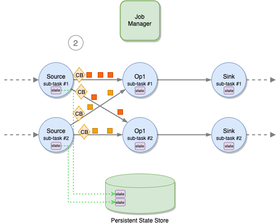
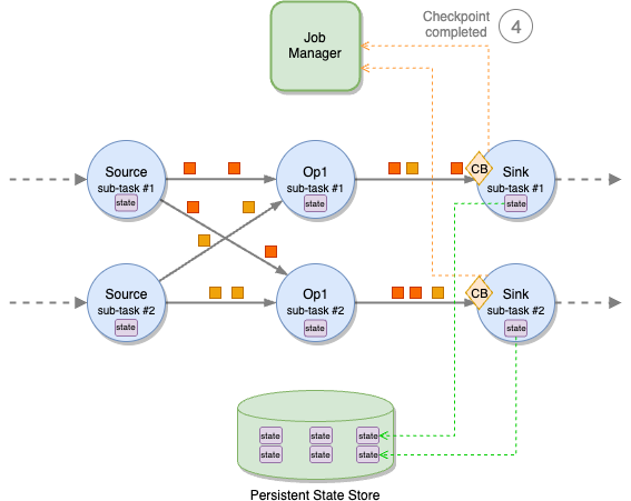
Data at rest directly managed by the service – Durable application storage (checkpoints and snapshots) and running application state storage (disk volumes used by RocksDB state backend) are automatically encrypted
Data in transit internal to the Flink cluster – Automatically encrypted using TLS/HTTPS
Data in transit to and at rest in external systems that your Flink application accesses – For example, an Amazon Managed Streaming for Apache Kafka (Amazon MSK) topic through the Kafka connector or calling an endpoint through a custom AsyncIO); encryption depends on the external service, user settings, and code

For data at rest managed by the service, checkpoints, snapshots, and running application state storage are encrypted by default using AWS owned keys. If your security requirements require you to directly control the encryption keys, you can use the CMK held in AWS KMS.

Key components and roles

To understand how CMKs work in Managed Service for Apache Flink, we first need to introduce the components and roles involved in managing and running an application using CMK encryption:

Customer managed key (CMK):
- Resides in AWS KMS within the same AWS account as your application
- Has an attached key policy that defines access permissions and usage rights to other components and roles
- Encrypts both durable application storage (checkpoints and snapshots) and running application state storage
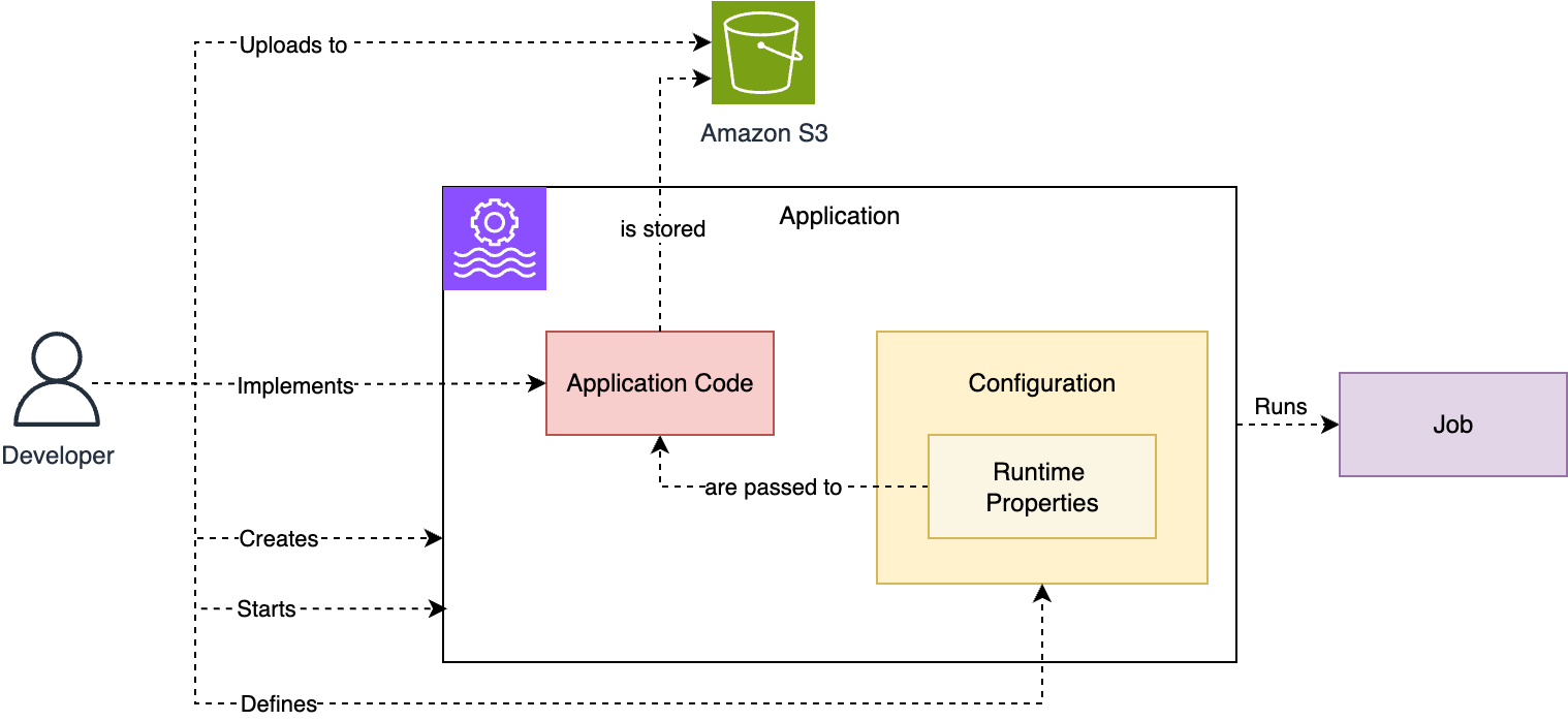
Managed Service for Apache Flink application:
- The application whose storage you want to encrypt using the CMK
- Has an attached AWS Identity and Access Management (IAM) execution role that grants permissions to access external services
- The execution role doesn’t have to provide any specific permissions to use the CMK for encryption operations
Key administrator:
- Manages the CMK lifecycle (creation, rotation, policy updates, and so on)
- Can be an IAM user or IAM role, and used by a human operator or by automation
- Requires administrative access to the CMK
- Permissions are defined by the attached IAM policies and the key policy
Application operator:
- Manages the application lifecycle (start/stop, configuration updates, snapshot management, and so on)
- Can be an IAM User or IAM role, and used by a human operator or by automation
- Requires permissions to manage the Flink application and use the CMK for encryption operations
- Permissions are defined by the attached IAM policies and the key policy

The following diagram illustrates the solution architecture.

Actors

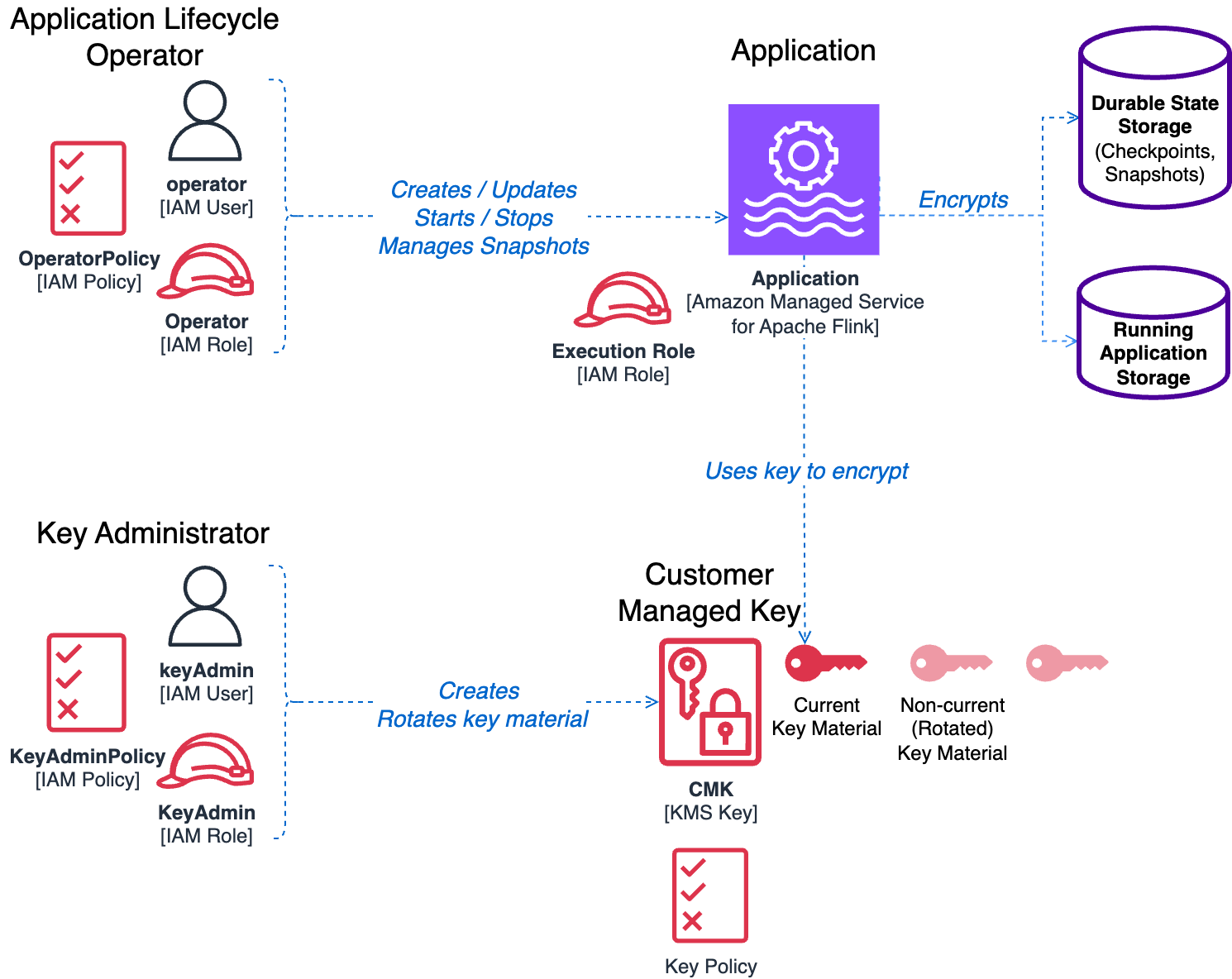
Enabling CMK following the principle of least privilege

When deploying applications in production environments or handling sensitive data, you should follow the principle of least privilege. CMK support in Managed Service for Apache Flink has been designed with this principle in mind, so each component receives only the minimum permissions necessary to function.

For detailed information about the permissions required by the application operator and key policy configurations, refer to Key management in Amazon Managed Service for Apache Flink. Although these policies might appear complex at first glance, this complexity is intentional and necessary. For more details about the requirements for implementing the most restrictive key management possible while maintaining functionality, refer to Least-privilege permissions.

For this post, we highlight some important points about CMK permissions:

Application execution role – Requires no additional permissions to use a CMK. You don’t need to change the permissions of an existing application; the service handles CMK operations transparently during runtime.
Application operator permissions – The operator is the user or role who controls the application lifecycle. For the permissions required to operate an application that uses CMK encryption, refer to Key management in Amazon Managed Service for Apache Flink. In addition to these permissions, an operator normally has permissions on actions with the kinesisanalytics prefix. It is a best practice to restrict these permissions to a specific application defining the Resource. The operator must also have the iam:PassRole permission to pass the service execution role to the application.

To simplify managing the permissions of the operator, we recommend creating two separate IAM policies, to be attached to the operator’s role or user:

A base operator policy defining the basic permissions to operate the application lifecycle without a CMK
An additional CMK operator policy that adds permissions to operate the application with a CMK

The following IAM policy example illustrates the permissions that should be included in the base operator policy:

{
  "Version": "2012-10-17",
  "Statement": [
    {
      "Sid": "Allow Managed Flink operations",
      "Effect": "Allow",
      "Action": "kinesisanalytics:*",
      "Resource": "arn:aws:kinesisanalytics:<region>:<account-id>:application/MyApplication"
    },
    {
      "Sid": "Allow passing service execution role",
      "Effect": "Allow",
      "Action": [
        "iam:PassRole"
      ],
      "Resource": "arn:aws:iam::<account-id>:role/MyApplicationRole"
    },
  ]
}

Refer to Application lifecycle operator (API caller) permissions for the permissions to be included with the additional CMK operator policy.

Separating these two policies has an additional benefit of simplifying the process of setting up an application for the CMK, due to the dependencies we illustrate in the following section.

Dependencies between the key policy and CMK operator policy

If you carefully observe the operator’s permissions and the key policy explained in Create a KMS key policy, you will notice some interdependencies, illustrated by the following diagram.

Dependencies

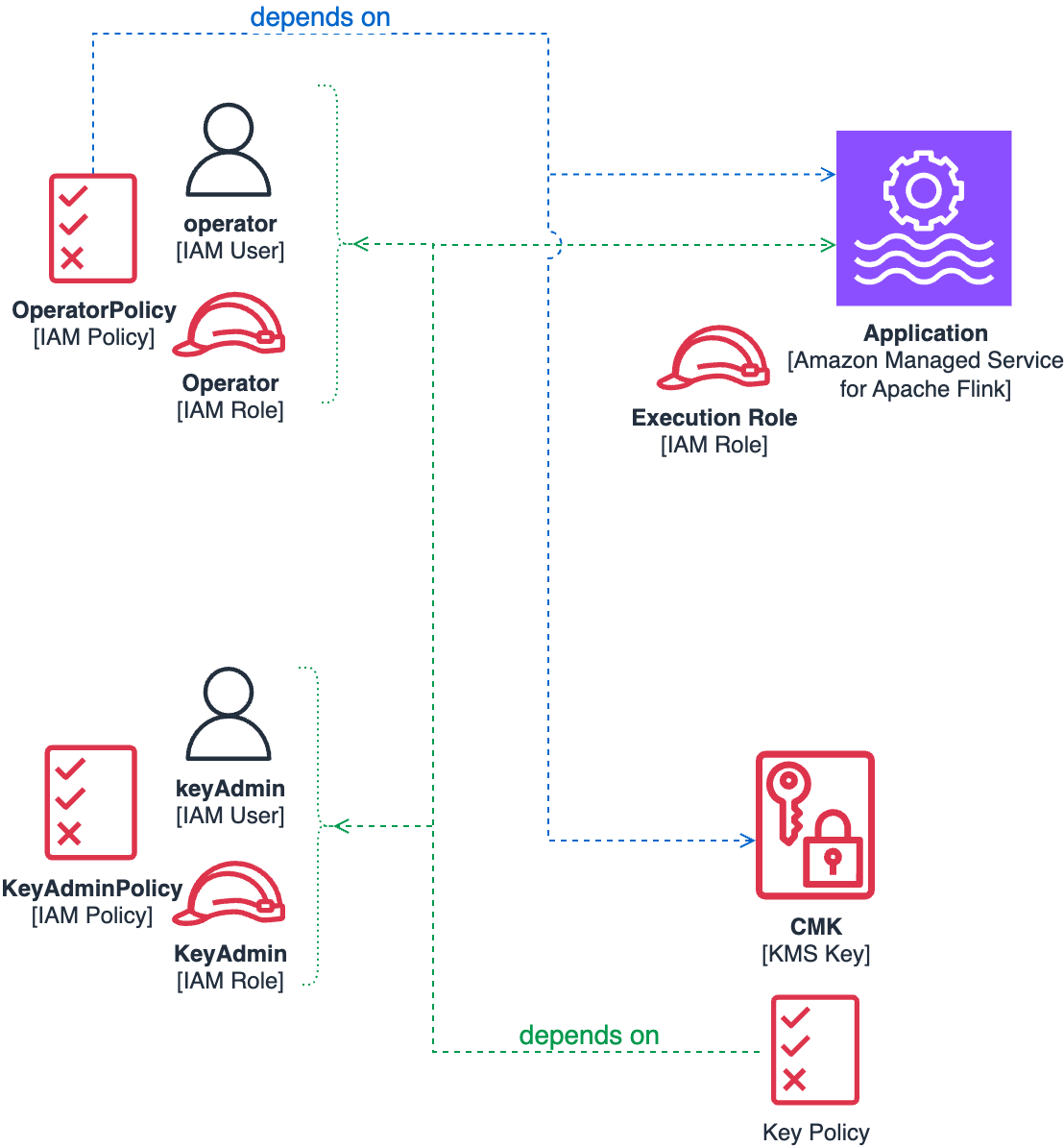
In particular, we highlight the following:

CMK key policy dependencies – The CMK policy requires references to both the application Amazon Resource Name (ARN) and the key administrator or operator IAM roles or users. This policy must be defined at key creation time by the key administrator.
IAM policy dependencies – The operator’s IAM policy must reference both the application ARN and the CMK key itself. The operator role is responsible for various tasks, including configuring the application to use the CMK.

To properly follow the principle of least privilege, each component requires the others to exist before it can be correctly configured. This necessitates a carefully orchestrated deployment sequence.

In the following section, we demonstrate the precise order required to resolve these dependencies while maintaining security best practices.

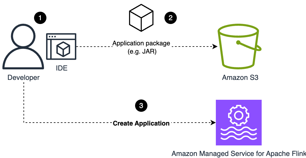
Sequence of operations to create a new application with a CMK

When deploying a new application that uses CMK encryption, we recommend following this sequenced approach to resolve dependency conflicts while maintaining security best practices:

Create the operator IAM role or user with a base policy that includes application lifecycle permissions. Do not include CMK permissions at this stage, because the key doesn’t exist yet.
The operator creates the application using the default AWS owned key. Keep the application in a stopped state to prevent data creation—there should be no data at rest to encrypt during this phase.
Create the key administrator IAM role or user, if not already available, with permissions to create and manage KMS keys. Refer to Using IAM policies with AWS KMS for detailed permission requirements.
The key administrator creates the CMK in AWS KMS. At this point, you have the required components for the key policy: application ARN, operator IAM role or user ARN, and key administrator IAM role or user ARN.
Create and attach to the operator an additional IAM policy that includes the CMK-specific permissions. See Application lifecycle operator (API caller) permissions for the complete operator policy definition.
The operator can now modify the application configuration using the UpdateApplication action, to enable CMK encryption, as illustrated in the following section.
The application is now ready to run with all data at rest encrypted using your CMK.

Enable the CMK with UpdateApplication

You can configure a Managed Service for Apache Flink application to use a CMK using the AWS Management Console, the AWS API, AWS Command Line Interface (AWS CLI), or infrastructure as code (IaC) tools like the AWS Cloud Development Kit (AWS CDK) or AWS CloudFormation templates.

When setting up CMK encryption in a production environment, you will probably use an automation tool rather than the console. These tools eventually use the AWS API under the hood, and the UpdateApplication action of the kinesisanalyticsv2 API in particular. In this post, we analyze the additions to the API that you can use to control the encryption configuration.

An additional top-level block ApplicationEncryptionConfigurationUpdate has been added to the UpdateApplication request payload. With this block, you can enable and disable the CMK.

You must add the following block to the UpdateApplication request:

{
  "ApplicationEncryptionConfigurationUpdate": {
    "KeyTypeUpdate": "CUSTOMER_MANAGED_KEY",
    "KeyIdUpdate": "arn:aws:kms:us-east-1:123456789012:key/01234567-99ab-cdef-0123-456789abcdef"
  }
}

The KeyIdUpdate value can be the key ARN, key ID, key alias name, or key alias ARN.

Disable the CMK

Similarly, the following requests disable the CMK, switching back to the default AWS owned key:

{
  "ApplicationEncryptionConfigurationUpdate": {
    "KeyTypeUpdate": "AWS_OWNED_KEY"
  }
}

Enable the CMK with CreateApplication

Theoretically, you can enable the CMK directly when you first create the application using the CreateApplication action.

A top-level block ApplicationEncryptionConfiguration has been added to the CreateApplication request payload, with a syntax similar to UpdateApplication.

However, due to the interdependencies described in the previous section, you will most often create an application with the default AWS owned key and later use UpdateApplication to enable the CMK.

If you omit ApplicationEncryptionConfiguration when you create the application, the default behavior is using the AWS owned key, for backward compatibility.

Sample CloudFormation templates to create IAM roles and the KMS key

The process you use to create the roles and key and configure the application to use the CMK will vary, depending on the automation you use and your approval and security processes. Any automation example we can provide will likely not fit your processes or tooling.

However, the following GitHub repository provides some example CloudFormation templates to generate some of the IAM policies and the KMS key with the correct key policy:

IAM policy for the key administrator – Allows managing the key
Base IAM policy for the operator – Allows managing the normal application lifecycle operations without the CMK
CMK IAM policy for the operator – Provides additional permissions required to manage the application lifecycle when the CMK is enabled
KMS key policy – Allows the application to encrypt and decrypt the application state and the operator to manage the application operations

CMK operations

We have described the process of creating a new Managed Service for Apache Flink application with CMK. Let’s now examine other common operations you can perform.

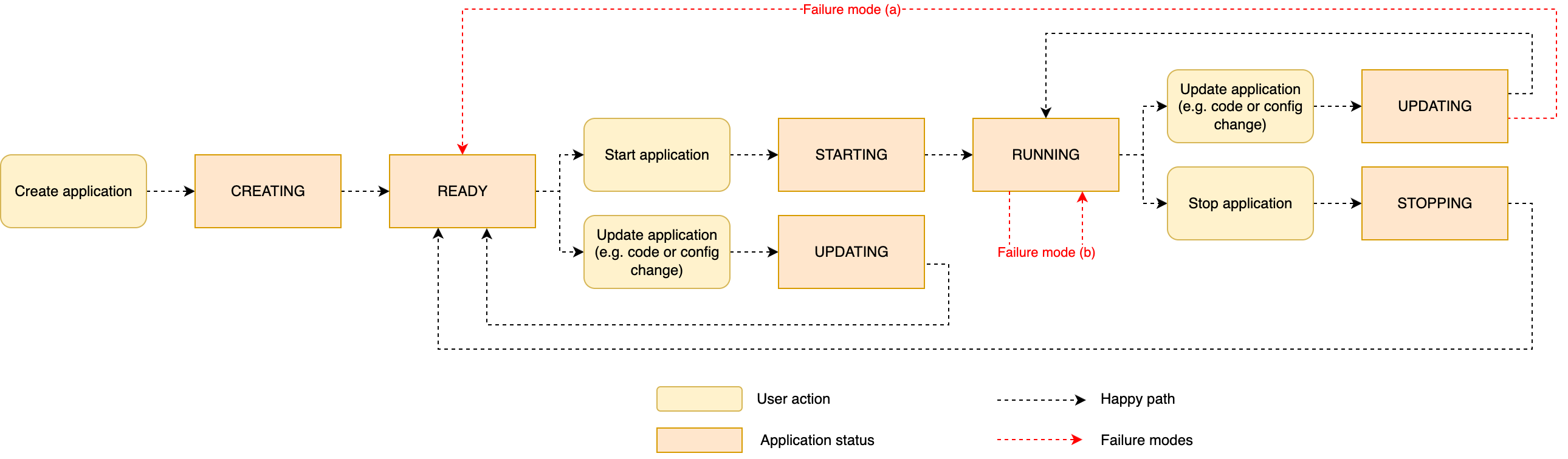
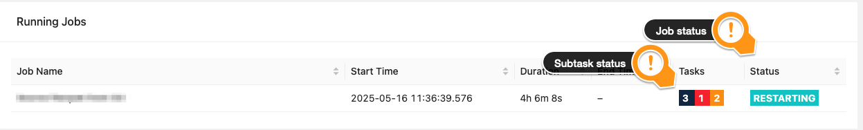
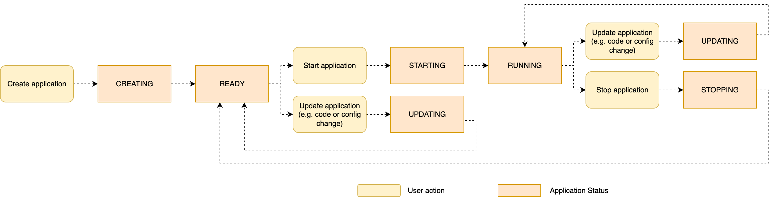
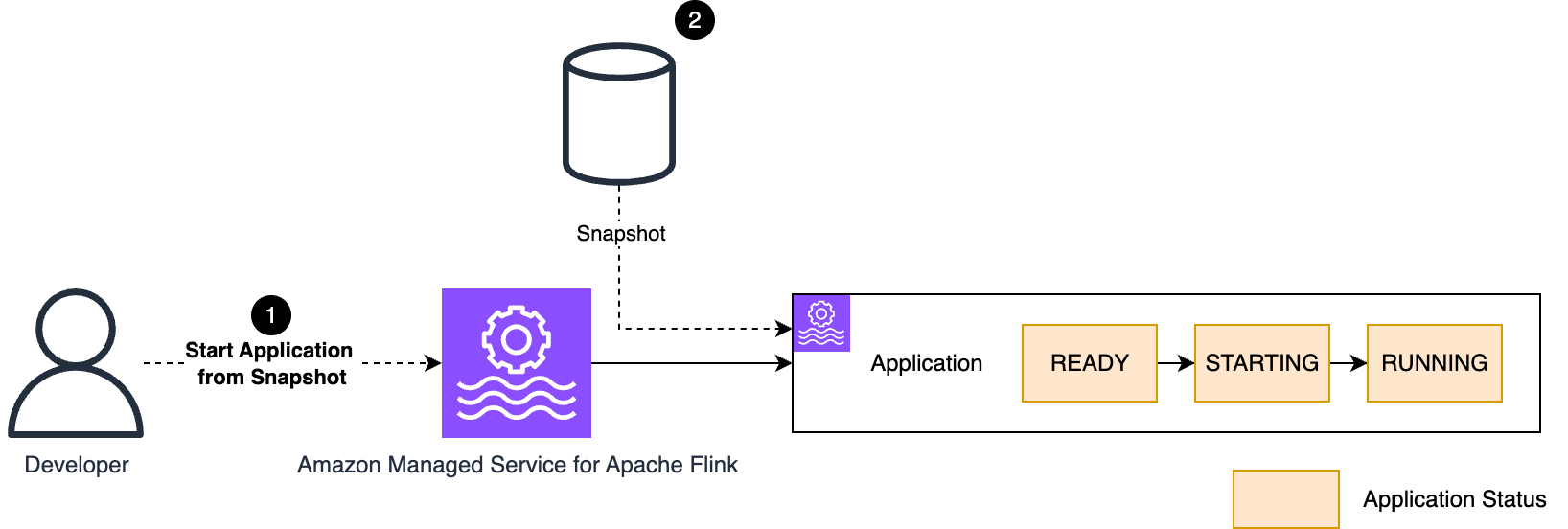
Changes to the encryption key become effective when the application is restarted. If you update the configuration of a running application, this causes the application to restart and the new key to be used immediately. Conversely, if you change the key of a READY (not running) application, the new key is not actually used until the application is restarted.

Enable a CMK on an existing application

If you have an application running with an AWS owned key, the process is similar to what we described for creating new applications. In this case, you already have a running application state and older snapshots that are encrypted using the AWS owned key.

Also, if you have a running application, you probably already have an operator role with an IAM policy that you can use to control the operator lifecycle.

The sequence of steps to enable a CMK on an existing and running application is as follows:

If you don’t already have one, create a key administrator IAM role or user with permissions to create and manage keys in AWS KMS. See Using IAM policies with AWS KMS for more details about the permissions required to manage keys.
The key administrator creates the CMK. The key policy references the application ARN, the operator’s ARN, and the key administrator’s role or user ARN.
Create an additional IAM policy that allows the use of the CMK and attach this policy to the operator. Alternatively, modify the operator’s existing IAM policy by adding these permissions.
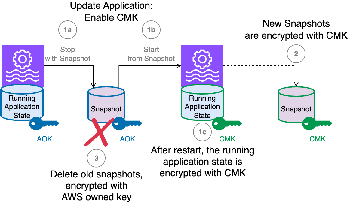
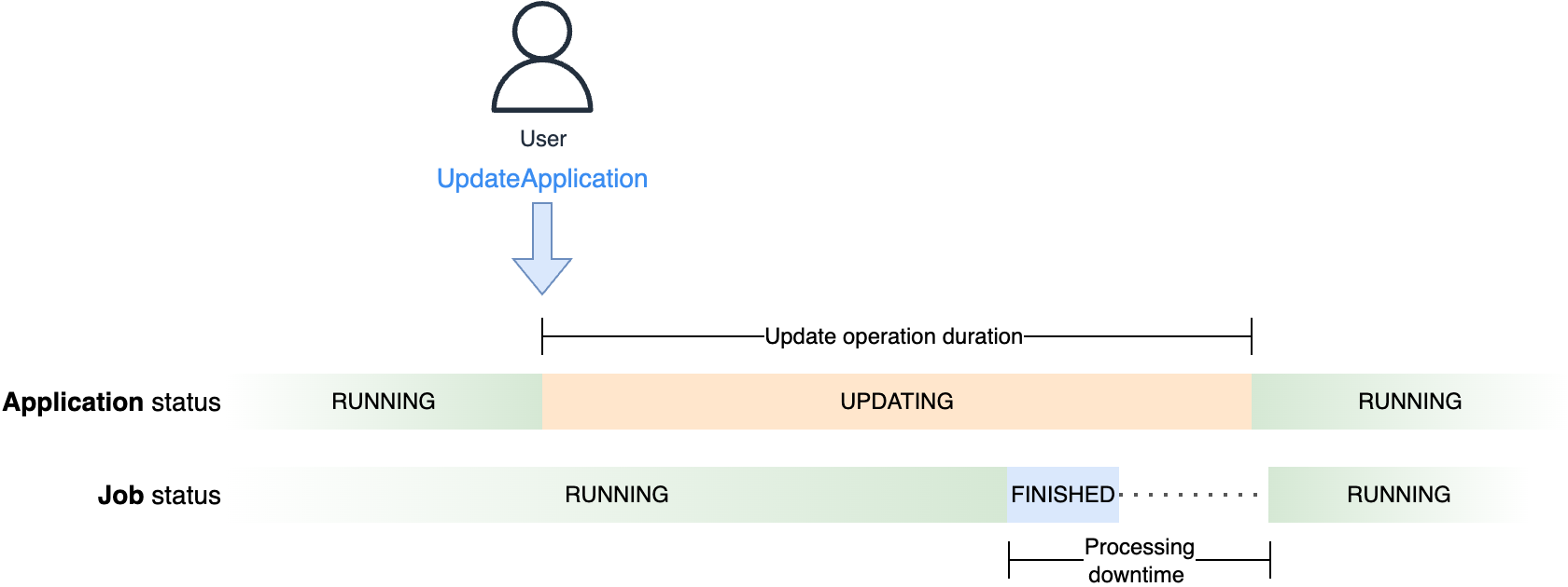
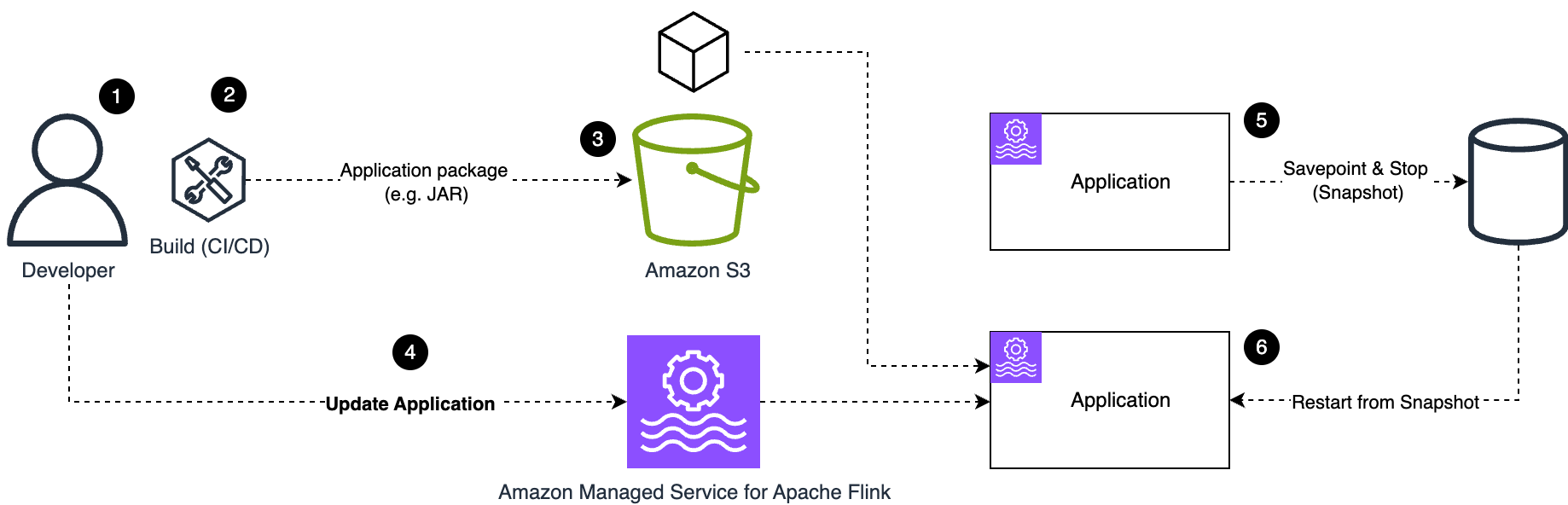
Finally, the operator can update the application and enable the CMK.The following diagram illustrates the process that occurs when you execute an UpdateApplication action on the running application to enable a CMK.

The workflow consists of the following steps:
When you update the application to set up the CMK, the following happens:
1. The application running state, at the moment it is encrypted with the AWS owned key, is saved in a snapshot while the application is stopped. This snapshot is encrypted with the default AWS owned key. The running application state storage is volatile and destroyed when the application is stopped.
2. The application is redeployed, restoring the snapshot into the running application state.
3. The running application state storage is now encrypted with the CMK.
New snapshots created from this point on are encrypted using the CMK.
You will probably want to delete all the old snapshots, including the one created automatically by the UpdateApplication that enabled the CMK, because they are all encrypted using the AWS owned key.

Rotate the encryption key

As with any cryptographic key, it’s a best practice to rotate the key periodically for enhanced security. Managed Service for Apache Flink does not support AWS KMS automatic key rotation, so you have two primary options for rotating your CMK.

Option 1: Create a new CMK and update the application

The first approach involves creating an entirely new KMS key and then updating your application configuration to use the new key. This method provides a clean separation between the old and new encryption keys, making it easier to track which data was encrypted with which key version.

Let’s assume you have a running application using CMK#1 (the current key) and want to rotate to CMK#2 (the new key) for enhanced security:

Prerequisites and preparation – Before initiating the key rotation process, you must update the operator’s IAM policy to include permissions for both CMK#1 and CMK#2. This dual-key access supports uninterrupted operation during the transition period. After the application configuration has been successfully updated and verified, you can safely remove all permissions to CMK#1.
Application update process – The UpdateApplication operation used to configure CMK#2 automatically triggers an application restart. This restart mechanism makes sure both the application’s running state and any newly created snapshots are encrypted using the new CMK#2, providing immediate security benefits from the updated encryption key.
Important security considerations – Existing snapshots, including the automatic snapshot created during the CMK update process, remain encrypted with the original CMK#1. For complete security hygiene and to minimize your cryptographic footprint, consider deleting these older snapshots after verifying that your application is functioning correctly with the new encryption key.

This approach provides a clean separation between old and new encrypted data while maintaining application availability throughout the key rotation process.

Option 2: Rotate the key material of the existing CMK

The second option is to rotate the cryptographic material within your existing KMS key. For a CMK used for Managed Service for Apache Flink, we recommend using on-demand key material rotation.

The benefit of this approach is simplicity: no change is required to the application configuration nor to the operator’s IAM permissions.

Important security considerations

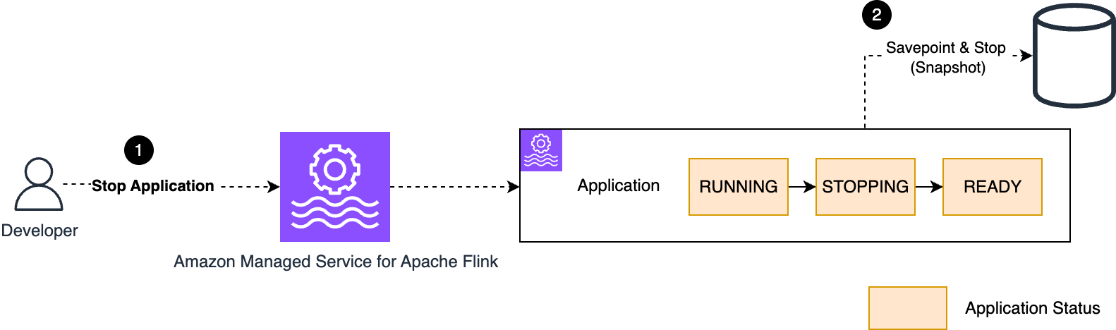
The new encryption key is used by the Managed Service for Apache Flink application only after the next application restart. To make the new key material effective, immediately after the rotation, you need to stop and start using snapshots to preserve the application state or execute an UpdateApplication, which also forces a stop-and-restart. After the restart, you should consider deleting the old snapshots, including the one taken automatically in the last stop-and-restart.

Switch back to the AWS owned key

At any time, you can decide to switch back to using an AWS owned key. The application state is still encrypted, but using the AWS owned key instead of your CMK.

If you are using the UpdateApplication API or AWS CLI command to switch back to CMK, you must explicitly pass ApplicationEncryptionConfigurationUpdate, setting the key type to AWS_OWNED_KEY as shown in the following snippet:

{
  "ApplicationEncryptionConfigurationUpdate": {
    "KeyTypeUpdate": "AWS_OWNED_KEY"
  }
}

When you execute UpdateApplication to switch off the CMK, the operator must still have permissions on the CMK. After the application is successfully running using the AWS owned key, you can safely remove any CMK-related permissions from the operator’s IAM policy.

Test the CMK in development environments

In a production environment—or an environment containing sensitive data—you should follow the principle of least privilege and apply the restrictive permissions described so far.

However, if you want to experiment with CMKs in a development setting, such as using the console, strictly following the production process might become cumbersome. In these environments, the roles of key administrator and operator are often filled by the same person.

For testing purposes in development environments, you might want to use a permissive key policy like the following, so you can freely experiment with CMK encryption:

{
  "Version": "2012-10-17",
  "Id": "key-policy-permissive-for-dev-only",
  "Statement": [
    {
      "Sid": "Allow any KMS action to Admin",
      "Effect": "Allow",
      "Principal": {
        "AWS": "arn:aws:iam::<account-id>:role/Admin"
      },
      "Action": "kms:*",
      "Resource": "*"
    },
    {
      "Sid": "Allow any KMS action to Managed Flink",
      "Effect": "Allow",
      "Principal": { 
        "Service": [
          "kinesisanalytics.amazonaws.com",
          "infrastructure.kinesisanalytics.amazonaws.com"
        ]
      },
      "Action": [
        "kms:DescribeKey",
        "kms:Decrypt",
        "kms:GenerateDataKey",
        "kms:GenerateDataKeyWithoutPlaintext",
        "kms:CreateGrant"
      ],
      "Resource": "*"
    }
  ]
}

This policy must never be used in an environment containing sensitive data, and especially not in production.

Common caveats and pitfalls

As discussed earlier, this feature is designed to maximize security and promote best practices such as the principle of least privilege. However, this focus can introduce some corner cases you should be aware of.

The CMK must be enabled for the service to encrypt and decrypt snapshots and running state

With AWS KMS, you can disable one key at any time. If you disable the CMK while the application is running, it might cause unpredictable failures. For example, an application will not be able to restore a snapshot if the CMK used to encrypt that snapshot has been disabled. For example, if you attempt to roll back an UpdateApplication that changed the CMK, and the previous key has since been disabled, you might not be able to restore from an old snapshot. Similarly, you might not be able to restart the application from an older snapshot if the corresponding CMK is disabled.

If you encounter these scenarios, the solution is to reenable the required key and retry the operation.

The operator requires permissions to all keys involved

To perform an action on the application (such as Start, Stop, UpdateApplication, or CreateApplicationSnapshot), the operator must have permissions for all CMKs involved in that operation. AWS owned keys don’t require explicit permission.

Some operations implicitly involve two CMKs—for example, when switching from one CMK to another, or when switching from a CMK to an AWS owned key by disabling the CMK. In these cases, the operator must have permissions for both keys for the operation to succeed.

The same rule applies when rolling back an UpdateApplication action that involved multiple CMKs.

A new encryption key takes effect only after restart

A new encryption key is only used after the application is restarted. This is important when you rotate the key material for a CMK. Rotating the key material in AWS KMS doesn’t require updating the Managed Flink application’s configuration. However, you must restart the application as a separate step after rotating the key. If you don’t restart the application, it will continue to use the old encryption key for its running state and snapshots until the next restart.

For this reason, it is recommended not to enable automatic key rotation for the CMK. When automatic rotation is enabled, AWS KMS might rotate the key material at any time, but your application will not start using the new key until it is next restarted.

CMKs are only supported with Flink runtime 1.20 or later

CMKs are only supported when you are using the Flink runtime 1.20 or later. If your application is currently using an older runtime, you should upgrade to Flink 1.20 first. Managed Service for Apache Flink makes it straightforward to upgrade your existing application using the in-place version upgrade.

Conclusion

Managed Service for Apache Flink provides robust security by enabling encryption by default, protecting both the running state and persistently saved state of your applications. For organizations that require full control over their encryption keys (often due to regulatory or internal policy needs), the ability to use a CMK integrated with AWS KMS offers a new level of assurance.

By using CMKs, you can tailor encryption controls to your specific compliance requirements. However, this flexibility comes with the need for careful planning: the CMK feature is intentionally designed to enforce the principle of least privilege and strong role separation, which can introduce complexity around permissions and operational processes.

In this post, we reviewed the key steps for enabling CMKs on existing applications, creating new applications with a CMK, and managing key rotation. Each of these processes gives you greater control over your data security but also requires attention to access management and operational best practices.

To get started with CMKs and for more comprehensive guidance, refer to Key management in Amazon Managed Service for Apache Flink.

About the authors

Deep dive into the Amazon Managed Service for Apache Fink application lifecycle – Part 2

2025-09-04 Lorenzo Nicora

Post Syndicated from Lorenzo Nicora original https://aws.amazon.com/blogs/big-data/part-2-deep-dive-into-the-amazon-managed-service-for-apache-fink-application-lifecycle/

In Part 1 of this series, we discussed fundamental operations to control the lifecycle of your Amazon Managed Service for Apache Flink application. If you are using higher-level tools such as AWS CloudFormation or Terraform, the tool will execute these operations for you. However, understanding the fundamental operations and what the service automatically does can provide some level of Mechanical Sympathy to confidently implement a more robust automation.

In the first part of this series, we focused on the happy paths. In an ideal world, failures don’t happen, and every change you deploy works perfectly. However, the real world is less predictable. Quoting Werner Vogels, Amazon’s CTO, “Everything fails, all the time.”

In this post, we explore failure scenarios that can happen during normal operations or when you deploy a change or scale the application, and how to monitor operations to detect and recover when something goes wrong.

The less happy path

A robust automation must be designed to handle failure scenarios, in particular during operations. To do that, we need to understand how Apache Flink can deviate from the happy path. Due to the nature of Flink as a stateful stream processing engine, detecting and resolving failure scenarios requires different techniques compared to other long-running applications, such as microservices or short-lived serverless functions (such as AWS Lambda).

Flink’s behavior on runtime errors: The fail-and-restart loop

When a Flink job encounters an unexpected error at runtime (an unhandled exception), the normal behavior is to fail, stop the processing, and restart from the latest checkpoint. Checkpoints allow Flink to support data consistency and no data loss in case of failure. Also, because Flink is designed for stream processing applications, which run continuously, if the error happens again, the default behavior is to keep restarting, hoping the problem is transient and the application will eventually recover the normal processing.In some cases, the problem is not transient, however. For example, when you deploy a code change that contains a bug, causing the job to fail as soon as it starts processing data, or if the expected schema doesn’t match the records in the source, causing deserialization or processing errors. The same scenario might also happen if you mistakenly changed a configuration that prevents a connector to reach the external system. In these cases, the job is stuck in a fail-and-restart loop, indefinitely, or until you actively force-stop it.

When this happens, the Managed Service for Apache Flink application status might be RUNNING, but the underlying Flink job is actually failing and restarting. The AWS Management Console gives you a hint, pointing that the application might need attention (see the following screenshot).

Application needs attention

In the following sections, we learn how to monitor the application and job status, to automatically react to this situation.

When starting or updating the application goes wrong

To understand the failure mode, let’s review what happens automatically when you start the application, or when the application restarts after you issued UpdateApplication command, as we explored in Part 1 of this series. The following diagram illustrates what happens when an application starts.

Application start process

The workflow consists of the following steps:

Managed Service for Apache Flink provisions a cluster dedicated to your application.
The code and configuration are submitted to the Job Manager node.
The code in the main() method of your application runs, defining the dataflow of your application.
Flink deploys to the Task Manager nodes the substasks that make up your job.
The job and application status change to RUNNING. However, subtasks start initializing now.
Subtasks restore their state, if applicable, and initialize any resources. For example, a Kafka connector’s subtask initializes the Kafka client and subscribes the topic.
When all subtasks are successfully initialized, they change to RUNNING status and the job starts processing data.

To new Flink users, it can be confusing that a RUNNING status doesn’t necessarily imply the job is healthy and processing data.When something goes wrong during the process of starting (or restarting) the application, depending on the phase when the problem arises, you might observe two different types of failure modes:

(a) A problem prevents the application code from being deployed – Your application might encounter this failure scenario if the deployment fails as soon as the code and configuration are passed to the Job Manager (step 2 of the process), for example if the application code package is malformed. A typical error is when the JAR is missing a mainClass or if mainClass points to a class that doesn’t exist. This failure mode might also happen if the code of your main() method throws an unhandled exception (step 3). In these cases, the application fails to change to RUNNING, and reverts to READY after the attempt.
(b) The application is started, the job is stuck in a fail-and-restart loop – A problem might occur later in the process, after the application status has changed RUNNING. For example, after the Flink job has been deployed to the cluster (step 4 of the process), a component might fail to initialize (step 6). This might happen when a connector is misconfigured, or a problem prevents it from connecting to the external system. For example, a Kafka connector might fail to connect to the Kafka cluster because of the connector’s misconfiguration or networking issues. Another possible scenario is when the Flink job successfully initializes, but it throws an exception as soon as it starts processing data (step 7). When this happens, Flink reacts to a runtime error and might get stuck in a fail-and-restart loop.

The following diagram illustrates the sequence of application status, including the two failure scenarios just described.

Application statuses, with failure scenarios

Troubleshooting

We have examined what can go wrong during operations, in particular when you update a RUNNING application or restart an application after changing its configuration. In this section, we explore how we can act on these failure scenarios.

Roll back a change

When you deploy a change and realize something is not quite right, you normally want to roll back the change and put the application back in working order, until you investigate and fix the problem. Managed Service for Apache Flink provides a graceful way to revert (roll back) a change, also restarting the processing from the point it was stopped before applying the fault change, providing consistency and no data loss.In Managed Service for Apache Flink, there are two types of rollbacks:

Automatic – During an automatic rollback (also called system rollback), if enabled, the service automatically detects when the application fails to restart after a change, or when the job starts but immediately falls into a fail-and-restart loop. In these situations, the rollback process automatically restores the application configuration version before the last change was applied and restarts the application from the snapshot taken when the change was deployed. See Improve the resilience of Amazon Managed Service for Apache Flink application with system-rollback feature for more details. This feature is disabled by default. You can enable it as part of the application configuration.
Manual – A manual rollback API operation is like a system rollback, but it’s initiated by the user. If the application is running but you observe something not behaving as expected after applying a change, you can trigger the rollback operation using the RollbackApplication API action or the console. Manual rollback is possible when the application is RUNNING or UPDATING.

Both rollbacks work similarly, restoring the configuration version before the change and restarting with the snapshot taken before the change. This prevents data loss and brings you back to a version of the application that was working. Also, this uses the code package that was saved at the time you created the previous configuration version (the one you are rolling back to), so there is no inconsistency between code, configuration, and snapshot, even if in the meantime you have replaced or deleted the code package from the Amazon Simple Storage Service (Amazon S3) bucket.

Implicit rollback: Update with an older configuration

A third way to roll back a change is to simply update the configuration, bringing it back to what it was before the last change. This creates a new configuration version, and requires the correct version of the code package to be available in the S3 bucket when you issue the UpdateApplication command.

Why is there a third option when the service provides system rollback and the managed RollbackApplication action? Because most high-level infrastructure-as-code (IaC) frameworks such as Terraform use this strategy, explicitly overwriting the configuration. It is important to understand this possibility even though you will probably use the managed rollback if you implement your automation based on the low-level actions.

The following are two important caveats to consider for this implicit rollback:

You will normally want to restart the application from the snapshot that was taken before the faulty change was deployed. If the application is currently RUNNING and healthy, this is not the latest snapshot (RESTORE_FROM_LATEST_SNAPSHOT), but rather the previous one. You must set the restart from RESTORE_FROM_CUSTOM_SNAPSHOT and select the correct snapshot.
UpdateApplication only works if the application is RUNNING and healthy, and the job can be gracefully stopped with a snapshot. Conversely, if the application is stuck in a fail-and-restart loop, you must force-stop it first, change the configuration while the application is READY, and later start the application from the snapshot that was taken before the faulty change was deployed.

Force-stop the application

In normal scenarios, you stop the application gracefully, with the automatic snapshot creation. However, this might not be possible in some scenarios, such as if the Flink job is stuck in a fail-and-restart loop. This might happen, for example, if an external system the job uses stops working, or because the AWS Identity and Access Management (IAM) configuration was erroneously modified, removing permissions required by the job.

When the Flink job gets stuck in a fail-and-restart loop after a faulty change, your first option should be using RollbackApplication, which automatically restores the previous configuration and starts from the correct snapshot. In the rare cases you can’t stop the application gracefully or use RollbackApplication, the last resort is force-stopping the application. Force-stop uses the StopApplication command with Force=true. You can also force-stop the application from the console.

When you force-stop an application, no snapshot is taken (if that were possible, you would have been able to gracefully stop). When you restart the application, you can either skip restoring from a snapshot (SKIP_RESTORE_FROM_SNAPSHOT) or use a snapshot that was previously taken, scheduled using Snapshot Manager, or manually, using the console or CreateApplicationSnapshot API action.

We strongly recommend setting up scheduled snapshots for all production applications that you can’t afford restarting with no state.

Monitoring Apache Flink application operations

Effective monitoring of your Apache Flink applications during and after operations is crucial to verify the outcome of the operation and allow lifecycle automation to raise alarms or react, in case something goes wrong.

The main indicators you can use during operations include the FullRestarts metric (available in Amazon CloudWatch) and the application, job, and task status.

Monitoring the outcome of an operation

The simplest way to detect the outcome of an operation, such as StartApplication or UpdateApplication, is to use the ListApplicationOperations API command. This command returns a list of the most recent operations of a specific application, including maintenance events that force an application restart.

For example, to retrieve the status of the most recent operation, you can use the following command:

aws kinesisanalyticsv2 list-application-operations \
    --application-name MyApplication \
   | jq '.ApplicationOperationInfoList \
   | sort_by(.StartTime) | last'

The output will be similar to the following code:

{
  "Operation": "UpdateApplication",
  "OperationId": "12abCDeGghIlM",
  "StartTime": "2025-08-06T09:24:22+01:00",
  "EndTime": "2025-08-06T09:26:56+01:00",
  "OperationStatus": "IN_PROGRESS"
}

OperationStatus will follow the same logic as the application status reported by the console and by DescribeApplication. This means it might not detect a failure during the operator initialization or while the job starts processing data. As we have learned, these failures might put the application in a fail-and-restart loop. To detect these scenarios using your automation, you must use other techniques, which we cover in the rest of this section.

Detecting the fail-and-restart loop using the FullRestarts metric

The simplest way to detect whether the application is stuck in a fail-and-restart loop is using the fullRestarts metric, available in CloudWatch Metrics. This metric counts the number of restarts of the Flink job after you started the application with a StartApplication command or restarted with UpdateApplication.

In a healthy application, the number of full restarts should ideally be zero. A single full restart might be acceptable during deployment or planned maintenance; multiple restarts normally indicate some issue. We recommend not to trigger an alarm on a single restart, or even a couple of consecutive restarts.

The alarm should only be triggered when the application is stuck in a fail-and-restart loop. This implies checking whether several restarts have happened over a relatively short period of time. Deciding the period is not trivial, because the time the Flink job takes to restart from a checkpoint depends on the size of the application state. However, if the state of your application is lower than several GB per KPU, you can safely assume the application should start in less than a minute.

The goal is creating a CloudWatch alarm that triggers when fullRestarts keeps increasing over a time period sufficient for multiple restarts. For example, assuming your application restarts in less than 1 minute, you can create a CloudWatch alarm that relies on the DIFF math expression of the fullRestarts metric. The following screenshot shows an example of the alarm details.

CloudWatch Alarm on fullRestarts

This example is a conservative alarm, only triggering if the application keeps restarting for over 5 minutes. This means you detect the problem after at least 5 minutes. You might consider reducing the time to detect the failure earlier. However, be careful not to trigger an alarm after just one or two restarts. Occasional restarts might happen, for example during normal maintenance (patching) that is managed by the service, or for a transient error of an external system. Flink is designed to recover from these conditions with minimal downtime and no data loss.

Detecting whether the job is up and running: Monitoring application, job, and task status

We have discussed how you have different statuses: the status of the application, job, and subtask. In Managed Service for Apache Flink, the application and job status change to RUNNING when the subtasks are successfully deployed on the cluster. However, the job is not really running and processing data until all the subtasks are RUNNING.

Observing the application status during operations

The application status is visible on the console, as shown in the following screenshot.

Screenshot: Application status

In your automation, you can poll the DescribeApplication API action to observe the application status. The following command shows how to use the AWS Command Line Interface (AWS CLI) and jq command to extract the status string of an application:

aws kinesisanalyticsv2 describe-application \ 
    --application-name <your-application-name> \
    | jq -r '.ApplicationDetail.ApplicationStatus'

Observing job and subtask status

Managed Service for Apache Flink gives you access to the Flink Dashboard, which provides useful information for troubleshooting, including the status of all subtasks. The following screenshot, for example, shows a healthy job where all subtasks are RUNNING.

Job and Task status

In the following screenshot, we can see a job where subtasks are failing and restarting.

Job status: failing

In your automation, when you start the application or deploy a change, you want to be sure the job is eventually up and running and processing data. This happens when all the subtasks are RUNNING. Note that waiting for the job status to become RUNNING after an operation is not completely safe. A subtask might still fail and cause the job to restart after it was reported as RUNNING.

After you execute a lifecycle operation, your automation can poll the substasks status waiting for one of two events:

All subtasks report RUNNING – This indicates the operation was successful and your Flink job is up and running.
Any subtask reports FAILING or CANCELED – This indicates something went wrong, and the application is likely stuck in a fail-and-restart loop. You need to intervene, for example, force-stopping the application and then rolling back the change.

If you are restarting from a snapshot and the state of your application is quite big, you might observe subtasks will report INITIALIZING status for longer. During the initialization, Flink restores the state of the operator before changing to RUNNING.

The Flink REST API exposes the state of the subtasks, and can be used in your automation. In Managed Service for Apache Flink, this requires three steps:

Generate a pre-signed URL to access the Flink REST API using the CreateApplicationPresignedUrl API action.
Make a GET request to the /jobs endpoint of the Flink REST API to retrieve the job ID.
Make a GET request to the /jobs/<job-id> endpoint to retrieve the status of the subtasks.

The following GitHub repository provides a shell script to retrieve the status of the tasks of a given Managed Service for Apache Flink application.

Monitoring subtasks failure while the job is running

The approach of polling the Flink REST API can be used in your automation, immediately after an operation, to observe whether the operation was eventually successful.

We strongly recommend not to continuously poll the Flink REST API while the job is running to detect failures. This operation is resource consuming, and might degrade performance or cause errors.

To monitor for suspicious subtask status changes during normal operations, we recommend using CloudWatch Logs instead. The following CloudWatch Logs Insights query extracts all subtask state transitions:

fields , message
| parse message /^(?<task>.+) switched from (?<fromStatus>[A-Z]+) to (?<toStatus>[A-Z]+)\./
| filter ispresent(task) and ispresent(fromStatus) and ispresent(toStatus)
| display , task, fromStatus, toStatus
| limit 10000

How Managed Service for Apache Flink minimizes processing downtime

We have seen how Flink is designed for strong consistency. To guarantee exactly-once state consistency, Flink temporarily stops the processing to deploy any changes, including scaling. This downtime is required for Flink to take a consistent copy of the application state and save it in a savepoint. After the change is deployed, the job is restarted from the savepoint, and there is no data loss. In Managed Service for Apache Flink, updates are fully managed. When snapshots are enabled, UpdateApplication automatically stops the job and uses snapshots (based on Flink’s savepoints) to retain the state.

Flink guarantees no data loss. However, your business requirements or Service Level Objectives (SLOs) might also impose a maximum delay for the data received by downstream systems, or end-to-end latency. This delay is affected by the processing downtime, or the time the job doesn’t process data to allow Flink deploying the change.With Flink, some processing downtime is unavoidable. However, Managed Service for Apache Flink is designed to minimize the processing downtime when you deploy a change.

We have seen how the service runs your application in a dedicated cluster, for complete isolation. When you issue UpdateApplication on a RUNNING application, the service prepares a new cluster with the required amount of resources. This operation might take some time. However, this doesn’t affect the processing downtime, because the service keeps the job running and processing data on the original cluster until the last possible moment, when the new cluster is ready. At this point, the service stops your job with a savepoint and restarts it on the new cluster.

During this operation, you are only charged for the number of KPU of a single cluster.

The following diagram illustrates the difference between the duration of the update operation, or the time the application status is UPDATING, and the processing downtime, observable from the job status, visible in the Flink Dashboard.

Downtime

You can observe this process, keeping both the application console and Flink Dashboard open, when you update the configuration of a running application, even with no changes. The Flink Dashboard will become temporarily unavailable when the service switches to the new cluster. Additionally, you can’t use the script we provided to check the job status for this scope. Even though the cluster keeps serving the Flink Dashboard until it’s tore down, the CreateApplicationPresignedUrl action doesn’t work while the application is UPDATING.

The processing time (the time the job is not running on either clusters) depends on the time the job takes to stop with a savepoint (snapshot) and restore the state in the new cluster. This time largely depends on the size of the application state. Data skew might also affect the savepoint time due to the barrier alignment mechanism. For a deep dive into the Flink’s barrier alignment mechanism, refer to Optimize checkpointing in your Amazon Managed Service for Apache Flink applications with buffer debloating and unaligned checkpoints, keeping in mind that savepoints are always aligned.

For the scope of your automation, you normally want to wait until the job is back up and running and processing data. You normally want to set a timeout. If both the application and job don’t return to RUNNING within this timeout, something probably went wrong and you might want to raise an alarm or force a rollback. This timeout should consider the entire update operation duration.

Conclusion

In this post, we discussed possible failure scenarios when you deploy a change or scale your application. We showed how Managed Service for Apache Flink rollback functionalities can seamlessly bring you back to a safe place after a change went wrong. We also explored how you can automate monitoring operations to observe application, job, and subtask status, and how to use the fullRestarts metric to detect when the job is in a fail-and-restart loop.

For more information, see Run a Managed Service for Apache Flink application, Implement fault tolerance in Managed Service for Apache Flink, and Manage application backups using Snapshots.

About the authors

Deep dive into the Amazon Managed Service for Apache Fink application lifecycle – Part 1

2025-09-04 Lorenzo Nicora

Post Syndicated from Lorenzo Nicora original https://aws.amazon.com/blogs/big-data/part-1-deep-dive-into-the-amazon-managed-service-for-apache-fink-application-lifecycle/

Apache Flink is an open source framework for stream and batch processing applications. It excels in handling real-time analytics, event-driven applications, and complex data processing with low latency and high throughput. Flink is designed for stateful computation with exactly-once consistency guarantees for the application state.

Amazon Managed Service for Apache Flink is a fully managed stream processing service that you can use to run Apache Flink jobs at scale without worrying about managing clusters and provisioning resources. You can focus on implementing your application using your integrated development environment (IDE) of choice, and build and package the application using standard build and continuous integration and delivery (CI/CD) tools.

With Managed Service for Apache Flink, you can control the application lifecycle through simple AWS API actions. You can use the API to start and stop the application, and to apply any changes to the code, runtime configuration, and scale. The service takes care of managing the underlying Flink cluster, giving you a serverless experience. You can implement automation such as CI/CD pipelines with tools that can interact with the AWS API or AWS Command Line Interface (AWS CLI).

You can control the application using the AWS Management Console, AWS CLI, AWS SDK, and tools using the AWS API, such as AWS CloudFormation or Terraform. The service is not prescriptive on the automation tool you use to deploy and orchestrate the application.

Paraphrasing Jackie Stewart, the famous racing driver, you don’t need to understand how to operate a Flink cluster to use Managed Service for Apache Flink, but some Mechanical Sympathy will help you implement a robust and reliable automation.

In this two-part series, we explore what happens during an application’s lifecycle. This post covers core concepts and the application workflow during normal operations. In Part 2, we look at potential failures, how to detect them through monitoring, and ways to quickly resolve issues when they occur.

Definitions

Before examining the application lifecycle steps, we need to clarify the usage of certain terms in the context of Managed Service for Apache Flink:

Application – The main resource you create, control, and run in Managed Service for Apache Flink is an application.
Application code package – For each Managed Service for Apache Flink application, you implement the application code package (application artifact) of the Flink application code you want to run. This code is compiled and packaged along with dependencies into a JAR or a ZIP file, that you upload to an Amazon Simple Storage Service (Amazon S3) bucket.
Configuration – Each application has a configuration that contains the information to run it. The configuration points to the application code package in the S3 bucket and defines the parallelism, which will also determine the application resources, in terms of KPUs. It also defines security, networking, and runtime properties, which are passed to your application code at runtime.
Job – When you start the application, Managed Service for Apache Flink creates a dedicated cluster for you and runs your application code as a Flink job.

The following diagram shows the relationship between these concepts.

Concepts

There are two additional important concepts: checkpoints and savepoints, the mechanisms Flink uses to guarantee state consistency across failures and operations. In Managed Service for Apache Flink, both checkpoints and savepoints are fully managed.

Checkpoints – These are controlled by the application configuration and enabled by default with a period of 1 minute. In Managed Service for Apache Flink, checkpoints are used when a job automatically restarts after a runtime failure. They are not durable and are deleted when the application is stopped or updated and when the application automatically scales.
Savepoints – These are called snapshots in Managed Service for Apache Flink, and are used to persist the application state when the application is deliberately restarted by the user, due to an update or an automatic scaling event. Snapshots can be triggered by the user. Snapshots (if enabled) are also automatically used to save and restore the application state when the application is stopped and restarted, for example to deploy a change or automatically scale. Automatic use of snapshots is enabled in the application configuration (enabled by default when you create an application using the console).

Lifecycle of an application in Managed Service for Apache Flink

Starting with the happy path, a typical lifecycle of a Managed Service for Apache Flink application comprises the following steps:

Create and configure a new application.
Start the application.
Deploy a change (update the runtime configuration, update the application code, change the parallelism to scale up or down).
Stop the application.

Starting, stopping, and updating the application use snapshots (if enabled) to retain application state consistency during operations. We recommend enabling snapshots on every production and staging application, to support the persistence of the application state across operations.

In Managed Service for Apache Flink, the application lifecycle is controlled through the console, API actions in the kinesisanalyticsv2 API, or equivalent actions in the AWS CLI and SDK. On top of these fundamental operations, you can build your own automation using different tools, directly using low-level actions or using higher level infrastructure-as-code (IaC) tooling such as AWS CloudFormation or Terraform.

In this post, we refer to the low-level API actions used at each step. Any higher-level IaC tooling will use combination of these operations. Understanding these operations is fundamental to designing a robust automation.

The following diagram summarizes the application lifecycle, showing typical operations and application statuses.

Application statuses

The status of your application, READY, STARTING, RUNNING, UPDATING, and so on, can be observed on the console and using the DescribeApplication API action.

In the following sections, we analyze each lifecycle operation in more detail.

Create and configure the application

The first step is creating a new Managed Service for Apache Flink application, including defining the application configuration. You can do this in a single step using the CreateApplication action, or by creating the basic application configuration and then updating the configuration before starting it using UpdateApplication. The latter approach is what you do when you create an application from the console.

In this phase, the developer packages the application they have implemented in a JAR file (for Java) or ZIP file (for Python) and uploads it to an S3 bucket the user has previously created. The bucket name and the path to the application code package are part of the configuration you define.

When UpdateApplication or CreateApplication is invoked, Managed Service for Apache Flink takes a copy of the application code package (JAR or ZIP file) referred by the configuration. The configuration is rejected if the file pointed by the configuration doesn’t exist.

The following diagram illustrates this workflow.

Create application

Simply updating the application code package in the S3 bucket doesn’t trigger an update. You need to run UpdateApplication to make the new file visible to the service and trigger the update, even when you overwrite the code package with the same name.

Start the application

Managed Service for Apache Flink provisions resources when the application is actually running, and you only pay for the resources of running applications. You explicitly control when to start the application by issuing a StartApplication.

Managed Service for Apache Flink indexes on high availability and runs your application in a dedicated Flink cluster. When you start the application, Managed Service for Apache Flink deploys a dedicated cluster and deploys and runs the Flink job based on the configuration you defined.

When you start the application, the status of the application moves from READY, to STARTING, and then RUNNING.

The following diagram illustrates this workflow.

Start application

Managed Service for Apache Flink supports both streaming mode, the default for Apache Flink, and batch mode:

Streaming mode – In streaming mode, after an application is successfully started and goes into RUNNING status, it keeps running until you stop it explicitly. From this point on, the behavior on failure is automatically restarting the job from the latest checkpoint, so there is no data loss. We discuss more details about this failure scenario later in this post.
Batch mode – A Flink application running in batch mode behaves differently. After you start it, it goes into RUNNING status, and the job continues running until it completes the processing. At that point the job will gracefully stop, and the Managed Service for Apache Flink application goes back to READY status.

This post focuses on streaming applications only.

Update the application

In Managed Service for Apache Flink, you handle the following changes by updating the application configuration, using the console or the UpdateApplication API action:

Application code changes, replacing the package (JAR or ZIP file) with one containing a new version
Runtime properties changes
Scaling, which implies changing parallelism and resources (KPU) changes
Operational parameter changes, such as checkpoint, logging level, and monitoring setup
Networking configuration changes

When you modify the application configuration, Managed Service for Apache Flink creates a new configuration version, identified by a version ID number, automatically incremented at every change.

Update the code package

We mentioned how the service takes a copy of the code package (JAR or ZIP file) when you update the application configuration. The copy is associated with the new application configuration version that has been created. The service uses its own copy of the code package to start the application. You can safely replace or delete the code package after you have updated the configuration. The new package is not taken into account until you update the application configuration again.

Update a READY (not running) application

If you update an application in READY status, nothing special happens beyond creating the new configuration version that will be used the next time you start the application. However, in production, you will normally update the configuration of an application in RUNNING status to apply a change. Managed Service for Apache Flink automatically handles the operations required to update the application with no data loss.

Update a RUNNING application

To understand what happens when you update a running application, you need to remember that Flink is designed for strong consistency and exactly-once state consistency. To maintain these features when a change is applied, Flink must stop the data processing, take a copy of the application state, restart the job with the changes, and restore the state, before processing can restart.

This is a standard Flink behavior, and applies to any changes, whether it’s code changes, runtime configuration changes, or new parallelism to scale up and down. Managed Service for Apache Flink automatically orchestrates this process for you. If snapshots are enabled, the service will take a snapshot before stopping the processing and restart from the snapshot when the change is deployed. This way, the change can be deployed with zero data loss.

If snapshots are disabled, the service restarts the job with the change, but the state will be empty, like the first time you started the application. This might cause data loss. You normally don’t want this to happen, particularly in production applications.

Let’s explore a practical example, illustrated by the following diagram. For instance, when you want to deploy a code change, the following steps typically happen (in this example, we assume that snapshots are enabled, which they should be in a production application):

Make changes to the application code.
The build process creates the application package (JAR or ZIP file), either manually or using CI/CD automation.
Upload the new application package to an S3 bucket.
Update the application configuration pointing to the new application package.
As soon as you successfully update the configuration, Managed Service for Apache Flink starts the operation for updating the application. The application status changes to UPDATING. The Flink job is stopped, taking a snapshot of the application state.
After the changes have been applied, the application is restarted using the new configuration, which in this case includes the new application code, and the job restores the state from the snapshot. When the process is complete, the application status goes back to RUNNING.

Update application

The process is similar for changes to the application configuration. For example, you can change the parallelism to scale the application updating the application configuration, causing the application to be redeployed with the new parallelism and the amount resources (CPU, memory, local storage) based on the new number of KPU.

Update the application’s IAM role

The application configuration contains a reference to an AWS Identity and Access Management (IAM) role. In the unlikely case you want to use a different role, you can update the application configuration using UpdateApplication. The process will be the same described earlier.

However, you usually want to modify the IAM role, to add or remove permissions. This operation doesn’t use the Managed Service for Apache Flink application lifecycle and can be done at any time. No application stop and restart is required. IAM changes take effect immediately, potentially inducing a failure if, for example, you inadvertently remove a required permission. In this case, the behavior of the Flink job’s response might vary, depending on the affected component.

Stop the application

You can stop a running Managed Service for Apache Flink application using the StopApplication action or the console. The service gracefully stops the application. The state turns from RUNNING, into STOPPING, and finally into READY.

When snapshots are enabled, the service will take a snapshot of the application state when it is stopped, as shown in the following diagram.

Stop application

After you stop the application, any resource previously provisioned to run your application is reclaimed. You incur no cost while the application is not running (READY).

Start the application from a snapshot

Sometimes, you might want to stop a production application and restart it later, restarting the processing from the point it was stopped. Managed Service for Apache Flink supports starting the application from a snapshot. The snapshot saves not only the application state, but also the point in the source—the offsets in a Kafka topic, for example—where the application stopped consuming.

When snapshots are enabled, Managed Service for Apache Flink automatically takes a snapshot when you stop the application. This snapshot can be used when you restart the application.

The StartApplication API command has three restore options:

RESTORE_FROM_LATEST_SNAPSHOT: Restore from the latest snapshot.
RESTORE_FROM_CUSTOM_SNAPSHOT: Restore from a custom snapshot (you need to specify which one).
SKIP_RESTORE_FROM_SNAPSHOT: Skip restoring from the snapshot. The application will start with no state, as the very first time you ran it.

When you start the application for the very first time, no snapshot is available yet. Regardless of the restore option you choose, the application will start with no snapshot.

The process of starting the application from a snapshot is visualized in the following diagram.

Start application with snapshot

In production, you normally want to restore from the latest snapshot (RESTORE_FROM_LATEST_SNAPSHOT). This will automatically use the snapshot the service created when you last stopped the application.

Snapshots are based on Flink’s savepoint mechanism and maintain the exactly-once consistency of the internal state. Also, the risk of reprocessing duplicate records from the source is minimized because the snapshot is taken synchronously while the Flink job is stopped.

Start the application from an older snapshot

In Managed Service for Apache Flink, you can schedule taking periodic snapshots of a running production application, for example using the Snapshot Manager. Taking a snapshot from a running application doesn’t stop the processing and only introduces a minimal overhead (comparable to checkpointing). With the second option, RESTORE_FROM_CUSTOM_SNAPSHOT, you can restart the application back in time, using a snapshot older than the one taken on the last StopApplication.

Because the source positions—for example, the offsets in a Kafka topic—are also restored with the snapshot, the application will revert to the point the application was processing when the snapshot was taken. This will also restore the state at that exact point, providing consistency.

When you start an application from an older snapshot, there are two important considerations:

Only restore snapshots taken within the source system retention period – If you restore a snapshot older than the source retention, data loss might occur, and the application behavior is unpredictable.
Restarting from an older snapshot will likely generate duplicate output – This is often not a problem when the end-to-end system is designed to be idempotent. However, this might cause problems if you are using a Flink transactional connector, such as File System sink or Kafka sink with exactly-once guarantees enabled. Because these sinks are designed to guarantee no duplicates (preventing them at any cost), they might prevent your application from restarting from an older snapshot. There are workarounds to this operational problem, but they depend on the specific use case and are beyond the scope of this post.

Understanding what happens when you start your application

We have learned the fundamental operations in the lifecycle of an application. In Managed Service for Apache Flink, these operations are controlled by a few API actions, such as StartApplication, UpdateApplication, and StopApplication. The service controls every operation for you. You don’t have to provision or manage Flink clusters. However, a better understanding of what happens during the lifecycle will give you sufficient Mechanical Sympathy to recognize potential failure modes and implement a more robust automation.

Let’s see in detail what happens when you issue a StartApplication command on an application in READY (not running). When you issue an UpdateApplication command on a RUNNING application, the application is first stopped with a snapshot, and then restarted with the new configuration, with a process identical to what we are going to see.

Composition of a Flink cluster

To understand what happens when you start the application, we need to introduce a couple of additional concepts. A Flink cluster is comprised of two types of nodes:

A single Job Manager, which acts as a coordinator
One or more Task Managers, which do the actual data processing

In Managed Service for Apache Flink, you can see the cluster nodes in the Flink Dashboard, which you can access from the console.

Flink decomposes the data processing defined by your application code into one or more subtasks, which are distributed across the Task Manager nodes, as illustrated in the following diagram.

Component of a Flink cluster

Remember, in Managed Service for Apache Flink, you don’t need to worry about provisioning and configuring the cluster. The service provides a dedicated cluster for your application. The total amount of vCPU, memory, and local storage of Task Managers matches the number of KPU you configured.

Starting your Managed Service for Apache Flink application

Now that we’ve discussed how a Flink cluster is composed, let’s explore what happens when you issue a StartApplication command, or when the application restarts after a change has been deployed with an UpdateApplication command.

The following diagram illustrates the process. Everything is carried out automatically for you.

Start application process

The workflow consists of the following steps:

A dedicated cluster, with the amount of resources you requested, based on the number of KPU, is provisioned for your application.
The application code, runtime properties, and other configurations such as the application parallelism are passed to the Job Manager node, the coordinator of the cluster.
The Java or Python code in the main() method of your application is executed. This generates the logical graph of operators of your application (called dataflow). Based on the dataflow you defined and the application parallelism, Flink generates the subtasks, the actual nodes Flink will execute to process your data.
Flink then distributes the job’s subtasks across Task Managers, the actual worker nodes of the cluster.
When the previous step succeeds, the Flink job status and the Managed Service for Apache Flink application status change to RUNNING. However, the job is still not completely running and processing data. All substasks must be initialized.
Each subtask independently restores its state, if starting from a snapshot, and initializes runtime resources. For example, Flink’s Kafka source connector restores the partition assignments and offsets from the savepoint (snapshot), establishes a connection to the Kafka cluster, and subscribes to the Kafka topic. From this step onward, a Flink job will stop and restart from its last checkpoint when encountering any unhandled error. If the problem causing the error is not transient, the job keeps stopping and restarting from the same checkpoint in a loop.
When all subtasks are successfully initialized and change to RUNNING status, the Flink job starts processing data and is now properly running.

Conclusion

In this post, we discussed how the lifecycle of a Managed Service for Apache Flink application is controlled by simple AWS API commands, or the equivalent using the AWS SDK or AWS CLI. If you are using high-level automation tools such as AWS CloudFormation or Terraform, the low-level actions are also abstracted away for you. The service handles the complexity of operating the Flink cluster and orchestrating the Flink job lifecycle.

However, with a better understanding of how Flink works and what the service does for you, you can implement more robust automation and troubleshoot failures.

In the Part 2, we continue examining failure scenarios that can happen during normal operations or when you deploy a change or scale the application, and how to monitor operations to detect and recover when something goes wrong.

About the authors

Unlock self-serve streaming SQL with Amazon Managed Service for Apache Flink

2025-05-28 Sofie Zilberman

Post Syndicated from Sofie Zilberman original https://aws.amazon.com/blogs/big-data/unlock-self-serve-streaming-sql-with-amazon-managed-service-for-apache-flink/

This post is co-written with Gal Krispel from Riskified.

Riskified is an ecommerce fraud prevention and risk management platform that helps businesses optimize online transactions by distinguishing legitimate customers from fraudulent ones.

Using artificial intelligence and machine learning (AI/ML), Riskified analyzes real-time transaction data to detect and prevent fraud while maximizing transaction approval rates. The platform provides a chargeback guarantee, protecting merchants from losses due to fraudulent transactions. Riskified’s solutions include account protection, policy abuse prevention, and chargeback management software, making it a comprehensive tool for reducing risk and enhancing customer experience. Businesses across various industries, including retail, travel, and digital goods, use Riskified to increase revenue while minimizing fraud-related losses. Riskified’s core business of real-time fraud prevention makes low-latency streaming technologies a fundamental part of its solution.

Businesses often can’t afford to wait for batch processing to make critical decisions. With real-time data streaming technologies like Apache Flink, Apache Spark, and Apache Kafka Streams, organizations can react instantly to emerging trends, detect anomalies, and enhance customer experiences. These technologies are powerful processing engines that perform analytical operations at scale. However, unlocking the full potential of streaming data often requires complex engineering efforts, limiting accessibility for analysts and business users.

Streaming pipelines are in high demand from Riskified’s Engineering department. Therefore, a user-friendly interface for creating streaming pipelines is a critical feature to increase analytical precision for detecting fraudulent transactions.

In this post, we present Riskified’s journey toward enabling self-service streaming SQL pipelines. We walk through the motivations behind the shift from Confluent ksqlDB to Apache Flink, the architecture Riskified built using Amazon Managed Service for Apache Flink, the technical challenges they faced, and the solutions that helped them make streaming accessible, scalable, and production-ready.

Using SQL to create streaming pipelines

Customers have a range of open source data processing technologies to choose from, such as Flink, Spark, ksqlDB, and RisingWave. Each platform offers a streaming API for data processing. SQL streaming jobs offer a powerful and intuitive way to process real-time data with minimal complexity. These pipelines use SQL, a widely known and declarative language, to perform real-time transformations, filtering, aggregations, and joins in continuous data streams.

To illustrate the power of streaming SQL in ecommerce fraud prevention, consider the concept of velocity checks, which are a critical fraud detection pattern. Velocity checks are a type of security measure used to detect unusual or rapid activity by monitoring the frequency and volume of specific actions within a given timeframe. These checks help identify potential fraud or abuse by analyzing repeated behaviors that deviate from normal user patterns. Common examples include detecting multiple transactions from the same IP address in a short time span, monitoring bursts of account creation attempts, or tracking the repeated use of a single payment method across different accounts.

Use case: Riskified’s velocity checks

Riskified implemented a real-time velocity check using streaming SQL to monitor purchasing behavior based on user identifier.

In this setup, transaction data is continuously streamed through a Kafka topic. Each message contains user agent information originating from the browser, along with the raw transaction data. Streaming SQL queries are used to aggregate the number of transactions originating from a single user identifier within short time windows.

For example, if the number of transactions from a given user identifier exceeds a certain threshold within a 10-second period, this might signal fraudulent activity. When that threshold is breached, the system can automatically flag or block the transactions before they are completed. The following figure and accompanying code provide a simplified example of the streaming SQL query used to detect this behavior.

Velocity check SQL flow

SELECT userIdentifier,TUMBLE_START(createdAt, INTERVAL '10' SECONDS) 
  AS windowStart,TUMBLE_END(createdAt, INTERVAL '10' SECONDS) 
  AS windowEnd, COUNT(*) AS paymentAttempts
FROM transactions
  WINDOW TUMBLING (SIZE 10 SECONDS)
GROUP BY userIdentifier;

Although defining SQL queries over static datasets might appear straightforward, developing and maintaining robust streaming applications introduces unique challenges. Traditional SQL operates on bounded datasets, which are finite collections of data stored in tables. In contrast, streaming SQL is designed to process continuous, unbounded data streams resembling the SQL syntax.

To address these challenges at scale and make streaming job creation accessible to engineering teams, Riskified implemented a self-serve solution based on Confluent ksqlDB, using its SQL interface and built-in Kafka integration. Engineers could define and deploy streaming pipelines using SQL, chaining ksqlDB streams from source to sink. The system supported both stateless and stateful processing directly on Kafka topics, with Avro schemas used to define the structure of streaming data.

Although ksqlDB provided a fast and approachable starting point, it eventually revealed several limitations. These included challenges with schema evolution, difficulties in managing compute resources, and the absence of an abstraction for managing pipelines as a cohesive unit. As a result, Riskified began exploring alternative technologies that could better support its expanding streaming use cases. The following sections outline these challenges in more detail.

Evolving the stream processing architecture

In evaluating alternatives, Riskified focused on technologies that could address the specific demands of fraud detection while preserving the simplicity that made the original approach appealing. The team encountered the following challenges in maintaining the previous solution:

Schemas are managed in Confluent Schema Registry, and the message format is Avro with FULL compatibility mode enforced. Schemas are constantly evolving according to business requirements. They are version controlled using Git with a strict continuous integration and continuous delivery (CI/CD) pipeline. As schemas grew more complex, ksqlDB’s approach to schema evolution didn’t automatically incorporate newly added fields. This behavior required dropping streams and recreating them to add new fields instead of just restarting the application to incorporate new fields. This approach caused inconsistencies with offset management due to the stream’s tear-down.
ksqlDB enforces a TopicNameStrategy schema registration strategy, which provides 1:1 schema-to-topic coupling. This means the exact schema definition has to be registered multiple times, one time for each topic it is used for. Riskified’s schema registry deployment uses RecordNameStrategy for schema registration. It’s an efficient schema registry strategy that allows for sharing schemas across multiple topics, storing fewer schemas, and reducing registry management overhead. Having mixed strategies in the schema registry caused errors with Kafka consumer clients attempting to decode messages, because the client implementation expected a RecordNameStrategy according to Riskified’s standard.
ksqlDB internally registers schema definitions in specific ways where fields are interpreted as nullable, and Avro Enum types are converted to Strings. This behavior caused deserialization errors when attempting to migrate native Kafka consumer applications to use the ksqlDB output topic. Riskified’s code base uses the Scala programming language, where optional fields in the schema are interpreted as Option. Transforming every field as optional in the schema definition required heavy refactoring, treating all Enum fields as Strings, and handling the Option data type for every field that requires safe handling. This cascading effect made the migration process more involved, requiring additional time and resources to achieve a smooth transition.

Managing resource contention in ksqlDB streaming workloads

ksqlDB queries are compiled into a Kafka Streams topology. The query definition defines the topology’s behavior.

Streaming query resources are shared rather than isolated. This approach typically leads to the overallocation of cluster resources. Its tasks are distributed across nodes in a ksqlDB cluster. This architecture means processing tasks with no resource isolation, and a specific task can impact other tasks running on the same node.

Resource contention between tasks on the same node is common in a production-intensive environment when using a cluster architecture solution. Operation teams often fine-tune cluster configurations to maintain acceptable performance, frequently mitigating issues by over-provisioning cluster nodes.

Challenges with ksqlDB pipelines

A ksqlDB pipeline is a chain of individual streams and lacks flow-level abstraction. Imagine a complex pipeline where a consumer publishes to multiple topics. In ksqlDB, each topic (both input and output) must be managed as a separate stream abstraction. However, there is no high-level abstraction to represent an entire pipeline that chains these streams together. As a result, engineering teams must manually assemble individual streams into a cohesive data flow, without built-in support for managing them as a single, complete pipeline.

This architectural approach particularly impacts operational tasks. Troubleshooting requires examining each stream separately, making it difficult to monitor and maintain pipelines that contain dozens of interconnected streams. When issues occur, the health of each stream needs to be checked individually, with no logical data flow component to help understand the relationships between streams or their role in the overall pipeline. The absence of a unified view of the data flow significantly increased operational complexity.

Flink as an alternative

Riskified began exploring alternatives for its streaming platform. The requirements were clear: a strong processing technology that combines a rich low-level API and a streaming SQL engine, backed by a strong open source community, proven to perform in the most demanding production environments.

Unlike the previous solution, which supported only Kafka-to-Kafka integration, Flink offers an array of connectors for various databases and Streaming platforms. It was quickly recognized that Flink had the potential to handle complex streaming use cases.

Flink offers multiple deployment options, including standalone clusters, native Kubernetes deployments using operators, and Hadoop YARN clusters. For enterprises seeking a fully managed option, cloud providers like AWS offer managed Flink services that help alleviate operational overhead, such as Managed Service for Apache Flink.

Benefits of using Managed Service for Apache Flink

Riskified decided to implement a solution using Managed Service for Apache Flink. This choice offered several key advantages:

It offers a quick and reliable way to run Flink applications and reduces the operational overhead of independently managing the infrastructure.
Managed Service for Apache Flink provides true job isolation by running each streaming application in its dedicated cluster. This means you can manage resources separately for each job and reduce the risk of heavy streaming jobs inflicting resource starvation for other running jobs.
It offers built-in monitoring using Amazon CloudWatch metrics, application state backup with managed snapshots, and automatic scaling.
AWS offers comprehensive documentation and practical examples to help accelerate the implementation process.

With these features, Riskified could focus on what truly matters—getting closer to the business goal and starting to write applications.

Using Flink’s streaming SQL engine

Developers can use Flink to build complex and scalable streaming applications, but Riskified saw it as more than just a tool for experts. They wanted to democratize the power of Flink into a tool for the entire organization, to solve complex business challenges involving real-time analytics requirements without needing a dedicated data professional.

To replace their previous solution, they envisioned maintaining a “build once, deploy many” application, which encapsulates the complexity of the Flink programming and allows the users to focus on the SQL processing logic.

Kafka was maintained as the input and output technology for the initial migration use case, which is similar to the ksqlDB setup. They designed a single, flexible Flink application where end-users can modify the input topics, SQL processing logic, and output destinations through runtime properties. Although ksqlDB primarily focuses on Kafka integration, Flink’s extensive connector ecosystem enables it to expand to diverse data sources and destinations in future phases.

Managed Service for Apache Flink provides a flexible way to configure streaming applications without modifying their code. By using runtime parameters, you can change the application’s behavior without modifying its source code.

Using Managed Service for Apache Flink for this approach includes the following steps:

Apply parameters for the input/output Kafka topic, a SQL query, and the input/output schema ID (assuming you’re using Confluent Schema Registry).
Use AvroSchemaConverter to convert an Avro schema into a Flink table.
Apply the SQL processing logic and save the output as a view.
Sink the view results into Kafka.

The following diagram illustrates this workflow.
Streaming SQL system diagram

Performing Flink SQL query compilation without a Flink runtime environment

Providing end-users with significant control to define their pipelines makes it critical to verify the SQL query defined by the user before deployment. This validation prevents failed or hanging jobs that could consume unnecessary resources and incur unnecessary costs.

A key challenge was validating Flink SQL queries without deploying the full Flink runtime. After investigating Flink’s SQL implementation, Riskified discovered its dependency on Apache Calcite – a dynamic data management framework that handles SQL parsing, optimization, and query planning independently of data storage. This insight enabled using Calcite directly for query validation before job deployment.

You must know how the data is structured to validate a Flink SQL query on a streaming source like a Kafka topic. Otherwise, unexpected errors might occur when attempting to query the streaming source. Although an expected schema is used with relational databases, it’s not enforced for streaming sources.

Schemas guarantee a deterministic structure for the data stored in a Kafka topic when using a schema registry. A schema can be materialized into a Calcite table that defines how data is structured in the Kafka topic. It allows inferring table structures directly from schemas (in this case, Avro format was used), enabling thorough field-level validation, including type checking and field existence, all before job deployment. This table can later be used to validate the SQL query.

The following code is an example of supporting basic field types validation using Calcite’s AbstractTable:

public class FlinkValidator {
    public static void validateSQL(String sqlQuery, Schema avroSchema) throws Exception {
        SqlParser.Config sqlConfig = SqlParser.config()
                .withCaseSensitive(true);
        SqlParser sqlParser = SqlParser.create(sqlQuery, sqlConfig);
        SqlNode parsedQuery = sqlParser.parseQuery();
        RelDataTypeFactory typeFactory = new SqlTypeFactoryImpl(RelDataTypeFactory.DEFAULT);
        CalciteSchema rootSchema = createSchemaWithAvro(avroSchema);
        SqlValidator validator = SqlValidatorUtil.newValidator(
                Frameworks.newConfigBuilder().build().getOperatorTable(),
                rootSchema.createCatalogReader(Collections.emptyList(), typeFactory),
                typeFactory,
                SqlValidator.Config.DEFAULT
        );
        validator.validate(parsedQuery);
    }
    private static CalciteSchema createSchemaWithAvro(Schema avroSchema) {
        CalciteSchema rootSchema = CalciteSchema.createRootSchema(true);
        rootSchema.add("TABLE", new SimpleAvroTable(avroSchema));
        return rootSchema;
    }
    private static class SimpleAvroTable extends org.apache.calcite.schema.impl.AbstractTable {
        private final Schema avroSchema;
        public SimpleAvroTable(Schema avroSchema) {
            this.avroSchema = avroSchema;
        }
        @Override
        public RelDataType getRowType(RelDataTypeFactory typeFactory) {
            RelDataTypeFactory.Builder builder = typeFactory.builder();
            for (Schema.Field field : avroSchema.getFields()) {
                builder.add(field.name(), convertAvroType(field.schema(), typeFactory));
            }
            return builder.build();
        }
        private RelDataType convertAvroType(Schema schema, RelDataTypeFactory typeFactory) {
            switch (schema.getType()) {
                case STRING:
                    return typeFactory.createSqlType(SqlTypeName.VARCHAR);
                case INT:
                    return typeFactory.createSqlType(SqlTypeName.INTEGER);
                default:
                    return typeFactory.createSqlType(SqlTypeName.ANY);
            }
        }
    }
}

You can integrate this validation approach as an intermediate step before creating the application. You can create a streaming job programmatically with the AWS SDK, AWS Command Line Interface (AWS CLI), or Terraform. The validation occurs before submitting the streaming job.

Flink SQL and Confluent Avro data type mapping limitation

Flink provides several APIs designed for different levels of abstraction and user expertise:

Flink SQL sits at the highest level, allowing users to express data transformations using familiar SQL syntax, which is ideal for analysts and teams comfortable with relational concepts.
The Table API offers a similar approach but is embedded in Java or Python, enabling type-safe and more programmatic expressions.
For more control, the DataStream API exposes low-level constructs to manage event time, stateful operations, and complex event processing.
At the most granular level, the ProcessFunction API provides full access to Flink’s runtime features. It’s suitable for advanced use cases that demand detailed control over state and processing behavior.

Riskified initially used the Table API to define streaming transformations. However, when deploying their first Flink job to a staging environment, they encountered serialization errors related to the avro-confluent library and Table API. Riskified’s schemas rely heavily on Avro Enum types, which the avro-confluent integration doesn’t fully support. As a result, Enum fields were converted to Strings, leading to mismatches during serialization and errors when attempting to sink processed data back to Kafka using Flink’s Table API.

Riskified developed an alternative approach to overcome the Enum serialization limitations while maintaining schema requirements. They discovered that Flink’s DataStream API could correctly handle Confluent’s Avro records serialization with Enum fields, unlike the Table API. They implemented a hybrid solution combining both APIs because the pipeline only required SQL processing on the source Kafka topic. It can sink to the output without any additional processing. The Table API is used for data processing and transformations, only converting to the DataStream API at the final output stage.

Managed Service for Apache Flink supports Flink APIs. It can switch between the Table API and the DataStream API.
A MapFunction can convert the Row type of the Table API into a DataStream of GenericRecord. The MapFunction maps Flink’s Row data type into GenericRecord types by iterating over the Avro schema fields and building the GenericRecord from the Flink Row type, casting the Row fields into the correct data type according to the Avro schema. This conversion is required to overcome the avro-confluent library limitation with Flink SQL.

The following diagram and illustrates this workflow.

Flink Table and DataStream APIs

The following code is an example query:

// SQL Query for filtering
Table queryResults = tableEnv.sqlQuery(
       "SELECT * FROM InputTable");
// 1. Convert query results from Table API to a DataStream<Row> and use DataStream API to sink query results to Kafka topic
DataStream<Row> rowStream = tableEnv.toDataStream(queryResults);
// Fetch the schema string from the schema registry
String schemaString = fetchSchemaString(schemaRegistryURL, schemaSubjectName);
// 2. Convert Row to GenericRecord with explicit TypeInformation, using custom AvroMapper
TypeInformation<GenericRecord> typeInfo = new GenericRecordAvroTypeInfo(avroSchema);
DataStream<GenericRecord> genericRecordStream = rowStream
       .map(new AvroMapper(schemaString))
       .returns(typeInfo); // Explicitly set TypeInformation
// 3. Define Kafka sink using ConfluentRegistryAvroSerializationSchema
KafkaSink<GenericRecord> kafkaSink = KafkaSink.<GenericRecord>builder()
       .setBootstrapServers(bootstrapServers)
       .setRecordSerializer(
               KafkaRecordSerializationSchema.builder()
                       .setTopic(sinkTopic)
                       .setValueSerializationSchema(
                               ConfluentRegistryAvroSerializationSchema.forGeneric(
                                       schemaSubjectName,
                                       avroSchema,
                                       schemaRegistryURL
                               )
                       )
                       .build()
       )
       .build();
// Sink to Kafka
genericRecordStream.sinkTo(kafkaSink);

CI/CD With Managed Service for Apache Flink

With Managed Service for Apache Flink, you can run a job by selecting an Amazon Simple Storage Service (Amazon S3) key containing the application JAR. Riskified’s Flink code base was structured as a multi-module repository to support additional use cases besides supporting self-service SQL. Each Flink job source code in the repository is an independent Java module. The CI pipeline implemented a robust build and deployment process consisting of the following steps:

Build and compile each module.
Run tests.
Package the modules.
Upload the artifact to the artifacts bucket twice: one JAR under <module>-<version>.jar and the second as <module>-latest.jar, resembling a Docker registry like Amazon Elastic Container Registry (Amazon ECR). Managed Service for Apache Flink jobs uses the latest tag artifact in this case. However, a copy of old artifacts is kept for code rollback reasons.

A CD process follows this process:

When merged, it lists all jobs for each module using the AWS CLI for Managed Service for Apache Flink.
The application JAR location is updated for each application, which triggers a deployment.
When the application is in a running state with no errors, the following application will be continued.

To allow safe deployment, this process is done gradually for every environment, starting with the staging environment.

Self-service interface for submitting SQL jobs

Riskified believes an intuitive UI is crucial for system adoption and efficiency. However, developing a dedicated UI for Flink job submission requires a pragmatic approach, because it might not be worth investing in unless there’s already a web interface for internal development operations.

Investing in UI development should align with the organization’s existing tools and workflows. Riskified had an internal web portal for similar operations, which made the addition of Flink job submission capabilities a natural extension of the self-service infrastructure.

An AWS SDK was installed on the web server to allow interaction with AWS components. The client receives user input from the UI and translates it into runtime properties to adjust the behavior of the Flink application. The web server then uses the CreateApplication API action to submit the job to Managed Service for Apache Flink.

Although an intuitive UI significantly enhances system adoption, it’s not the only path to accessibility. Alternatively, a well-designed CLI tool or REST API endpoint can provide the same self-service capabilities.

The following diagram illustrates this workflow.

Flow sequence diagram

Production experience: Flink’s implementation upsides

The transition to Flink and Managed Service for Apache Flink proved efficient in numerous aspects:

Schema evolution and data handling – Riskified can either periodically fetch updated schemas or restart applications when schemas evolve. They can use existing schemas without self-registration.
Resource isolation and management – Managed Service for Apache Flink runs each Flink job as an isolated cluster, reducing resource contention between jobs.
Resource allocation and cost-efficiency – Managed Service for Apache Flink enables minimum resource allocation with automatic scaling, proving to be more cost-efficient.
Job management and flow visibility – Flink provides a cohesive data flow abstraction through its job and task model. It manages the entire data flow in a single job and distributes the workload evenly over multiple nodes. This unified approach enables better visibility into the entire data pipeline, simplifying monitoring, troubleshooting, and optimizing complex streaming workflows.
Built-in recovery mechanism – Managed Service for Apache Flink automatically creates checkpoints and savepoints that enable stateful Flink applications to recover from failures and resume processing without data loss. With this feature, streaming jobs are durable and can recover safely from errors.
Comprehensive observability – Managed Service for Apache Flink exposes CloudWatch metrics that monitor Flink application performance and statistics. You can also create alarms based on these metrics. Riskfied decided to use the Cloudwatch Prometheus Exporter to export these metrics to Prometheus and build PrometheusRules to align Flink’s monitoring to the Riskified standard, which uses Prometheus and Grafana for monitoring and alerting.

Next steps

Although the initial focus was Kafka-to-Kafka streaming queries, Flink’s wide range of sink connectors offers the possibility of pluggable multi-destination pipelines. This versatility is on Riskfied’s roadmap for future enhancements.

Flink’s DataStream API provides capabilities that extend far beyond self-serving streaming SQL capabilities, opening new avenues for more sophisticated fraud detection use cases. Riskified is exploring ways to use DataStream APIs to enhance ecommerce fraud prevention strategies.

Conclusions

In this post, we shared how Riskified successfully transitioned from ksqlDB to Managed Service for Apache Flink for its self-serve streaming SQL engine. This move addressed key challenges like schema evolution, resource isolation, and pipeline management. Managed Service for Apache Flink offers features such as including isolated jobs environments, automatic scaling, and built-in monitoring, which proved more efficient and cost-effective. Although Flink SQL limitations with Kafka required workarounds, using Flink’s DataStream API and user-defined functions resolved these issues. The transition has paved the way for future expansion with multi-targets and advanced fraud detection capabilities, solidifying Flink as a robust and scalable solution for Riskified’s streaming needs.

If Riskified’s journey has sparked your interest in building a self-service streaming SQL platform, here’s how to get started:

Learn more about Managed Service for Apache Flink:
Get hands-on experience:
- Amazon Managed Service for Apache Flink Workshop
- Amazon Managed Service for Apache Flink Examples

About the authors

Gal Krispel is a Data Platform Engineer at Riskified, specializing in streaming technologies such as Apache Kafka and Apache Flink. He focuses on building scalable, real-time data pipelines that power Riskified’s core products. Gal is particularly interested in making complex data architectures accessible and efficient across the organization. His work spans real-time analytics, event-driven design, and the seamless integration of stream processing into large-scale production systems.

Sofia Zilberman works as a Senior Streaming Solutions Architect at AWS, helping customers design and optimize real-time data pipelines using open-source technologies like Apache Flink, Kafka, and Apache Iceberg. With experience in both streaming and batch data processing, she focuses on making data workflows efficient, observable, and high-performing.

Lorenzo Nicora works as Senior Streaming Solution Architect at AWS, helping customers across EMEA. He has been building cloud-centered, data-intensive systems for over 25 years, working across industries both through consultancies and product companies. He has used open-source technologies extensively and contributed to several projects, including Apache Flink, and is the maintainer of the Flink Prometheus connector.

Process millions of observability events with Apache Flink and write directly to Prometheus

2025-04-09 Lorenzo Nicora

Post Syndicated from Lorenzo Nicora original https://aws.amazon.com/blogs/big-data/process-millions-of-observability-events-with-apache-flink-and-write-directly-to-prometheus/

AWS recently announced support for a new Apache Flink connector for Prometheus. The new connector, contributed by AWS to the Flink open source project, adds Prometheus and Amazon Managed Service for Prometheus as a new destination for Flink.

In this post, we explain how the new connector works. We also show how you can manage your Prometheus metrics data cardinality by preprocessing raw data with Flink to build real-time observability with Amazon Managed Service for Prometheus and Amazon Managed Grafana.

Amazon Managed Service for Prometheus is a secure, serverless, scaleable, Prometheus-compatible monitoring service. You can use the same open source Prometheus data model and query language that you use today to monitor the performance of your workloads without having to manage the underlying infrastructure. Flink connectors are software components that move data into and out of an Amazon Managed Service for Apache Flink application. You can use the new connector to send processed data to an Amazon Managed Service for Prometheus destination starting with Flink version 1.19. With Amazon Managed Service for Apache Flink, you can transform and analyze data in real time. There are no servers and clusters to manage, and there is no compute and storage infrastructure to set up.

Observability beyond compute

In an increasingly connected world, the boundary of systems extends beyond compute assets, IT infrastructure, and applications. Distributed assets such as Internet of Things (IoT) devices, connected cars, and end-user media streaming devices are an integral part of business operations in many sectors. The ability to observe every asset of your business is key to detecting potential issues early, improving the experience of your customers, and protecting the profitability of the business.

Metrics and time series

It is helpful to think of observability as three pillars: metrics, logs, and traces. The most relevant pillar for distributed devices, like IoT, is metrics. This is because metrics can capture measurements from sensors or counting of specific events emitted by the device.

Metrics are series of samples of a given measurement at specific times. For example, in the case of a connected vehicle, they can be the readings from the electric motor RPM sensor. Metrics are normally represented as time series, or sequences of discrete data points in chronological order. Metrics’ time series are normally associated with dimensions, also called labels or tags, to help with classifying and analyzing the data. In the case of a connected vehicle, labels might be something like the following:

Metric name – For example, “Electric Motor RPM”
Vehicle ID – A unique identifier of the vehicle, like the Vehicle Identification Number (VIN)

Prometheus as a specialized time series database

Prometheus is a popular solution for storing and analyzing metrics. Prometheus defines a standard interface for storing and querying time series. Commonly used in combination with visualization tools like Grafana, Prometheus is optimized for real-time dashboards and real-time alerting.

Often considered mainly for observing compute resources, like containers or applications, Prometheus is actually a specialized time series database that can effectively be used to observe different types of distributed assets, including IoT devices.

Amazon Managed Service for Prometheus is a serverless, Prometheus-compatible monitoring service. See What is Amazon Managed Service for Prometheus? to learn more about Amazon Managed Service for Prometheus.

Effectively processing observability events, at scale

Handling observability data at scale becomes more challenging, due to the number of assets and unique metrics, especially when observing massively distributed devices, for the following reasons:

High cardinality – Each device emits multiple metrics or types of events, each to be tracked independently.
High frequency – Devices might emit events very frequently, multiple times per second. This might result in a large volume of raw data. This aspect in particular represents the main difference from observing compute resources, which are usually scraped at longer intervals.
Events arrive at irregular intervals and out of order – Unlike compute assets that are usually scraped at regular intervals, we often see delays of transmission or temporarily disconnected devices, which cause events to arrive at irregular intervals. Concurrent events from different devices might follow different paths and arrive at different times.
Lack of contextual information – Devices often transmit over channels with limited bandwidth, such as GPRS or Bluetooth. To optimize communication, events seldom contain contextual information, such as device model or user detail. However, this information is required for an effective observability.
Derive metrics from events – Devices often emit specific events when specific facts happen. For example, when the vehicle ignition is turned on or off, or when a warning is emitted by the onboard computer. These are not direct metrics. However, counting and measuring the rates of these events are valuable metrics that can be inferred from these events.

Effectively extracting value from raw events requires processing. Processing might happen on read, when you query the data, or upfront, before storing.

Storing and analyzing raw events

The common approach with observability events, and with metrics in particular, is “storing first.” You can simply write the raw metrics into Prometheus. Processing, such as grouping, aggregating, and calculating derived metrics, happens “on query,” when data is extracted from Prometheus.

This approach might become particularly inefficient when you’re building real-time dashboards or alerting, and your data has very high cardinality or high frequency. As a time series database is continuously queried, a large volume of data is repeatedly extracted from the storage and processed. The following diagram illustrates this workflow.

Process on query

Preprocessing raw observability events

Preprocessing raw events before storing shifts the work left, as illustrated in the following diagram. This increases the efficiency of real-time dashboards and alerts, allowing the solution to scale.

Pre-process

Apache Flink for preprocessing observability events

Preprocessing raw observability events requires a processing engine that allows you to do the following:

Enrich events efficiently, looking up reference data and adding new dimensions to the raw events. For example, adding the vehicle model based on the vehicle ID. Enrichment allows adding new dimensions to the time series, enabling analysis otherwise impossible.
Aggregate raw events over time windows, to reduce frequency. For example, if a vehicle emits an engine temperature measurement every second, you can emit a single sample with the average over 5 seconds. Prometheus can efficiently aggregate frequent samples on read. However, ingesting data with a frequency much higher than what is useful for dashboarding and real-time alerting is not an efficient use of Prometheus ingestion throughout and storage.
Aggregate raw events over dimensions, to reduce cardinality. For example, aggregating some measurement per vehicle model.
Calculate derived metrics applying arbitrary logic. For example, counting the number of warning events emitted by each vehicle. This also enables analysis otherwise impossible using only Prometheus and Grafana.
Support event-time semantics, to aggregate over time events from different sources.

Such a preprocessing engine must also be able to scale and process the large volume of input raw events, and to process data with low latency—normally subsecond or single-digit seconds—to enable real-time dashboards and altering. To address these requirements, we see many customers using Flink.

Apache Flink meets the aforementioned requirements. Flink is a framework and distributed stream processing engine, designed to perform computations at in-memory speed and at scale. Amazon Managed Service for Apache Flink offers a fully managed, serverless experience, allowing you to run your Flink applications without managing infrastructure or clusters.

Amazon Managed Service for Apache Flink can process the ingested raw events. The resulting metrics, with lower cardinality and frequency, and additional dimensions, can be written to Prometheus for a more effective visualization and analysis. The following diagram illustrates this workflow.

Amazon Managed Service for Apache Flink, Amazon Managed Prometheus and Grafana

Integrating Apache Flink and Prometheus

The new Flink Prometheus connector allows Flink applications to seamlessly write preprocessed time series data to Prometheus. No intermediate component is needed, and there is no requirement to implement a custom integration. The connector is designed to scale, using the ability of Flink to scale horizontally, and optimizing the writes to a Prometheus backend using a Remote-Write interface.

Example use case

AnyCompany is a car rental company managing a fleet of hundreds of thousands hybrid connected vehicles, in multiple regions. Each vehicle continuously transmits measurements from several sensors. Each sensor emits a sample every second or more frequently. Vehicles also communicate warning events when something wrong is detected by the onboard computer. The following diagram illustrates the workflow.

Example use case: connected cars

AnyCompany is planning to use Amazon Managed Service for Prometheus and Amazon Managed Grafana to visualize vehicle metrics and set up custom alerts.

However, building a real-time dashboard based on raw data, as transmitted by the vehicles, might be complicated and inefficient. Each vehicle might have hundreds of sensors, each of them resulting in a separate time series to display. Additionally, AnyCompany wants to monitor the behavior of different vehicle models. Unfortunately, the events transmitted by the vehicles only contain the VIN. The model can be inferred by looking up (joining) some reference data.

To overcome these challenges, AnyCompany has built a preprocessing stage based on Amazon Managed Service for Apache Flink. This stage has the following capabilities:

Enrich the raw data by adding the vehicle model, and looking up reference data based on the vehicle identification.
Reduce the cardinality, aggregating the results per vehicle model, available after the enrichment step.
Reduce the frequency of the raw metrics to reduce write bandwidth, aggregating over time windows of a few seconds.
Calculate derived metrics based on multiple raw metrics. For example, determine whether a vehicle is in motion when either the internal combustion engine or the electrical motor are rotating.

The result of preprocessing are more actionable metrics. A dashboard built on these metrics can, for example, help determine whether the last software update released over-the-air to all vehicles of a specific model in specific regions, is causing issues.

Using the Flink Prometheus connector, the preprocessor application can write directly to Amazon Managed Service for Prometheus, without intermediate components.

Nothing prevents you from choosing to write raw metrics with full cardinality and frequency to Prometheus, allowing you to drill down to the single vehicle. The Flink Prometheus connector is designed to scale by batching and parallelizing writes.

Solution overview

The following GitHub repository contains a fictional end-to-end example covering this use case. The following diagram illustrates the architecture of this example.

Example architecture

The workflow consists of the following steps:

Vehicles, radio transmission, and ingestion of IoT events have been abstracted away, and replaced by a data generator that produces raw events for a hundred thousand fictional vehicles. For simplicity, the data generator is itself an Amazon Managed Service for Apache Flink application.
Raw vehicle events are sent to a stream storage service. In this example, we use Amazon Managed Streaming for Apache Kafka (Amazon MSK).
The core of the system is the preprocessor application, running in Amazon Managed Service for Apache Flink. We will dive deeper into the details of the processor in the following sections.
Processed metrics are directly written to the Prometheus backend, in Amazon Managed Service for Prometheus.
Metrics are used to generate real-time dashboards on Amazon Managed Grafana.

The following screenshot shows a sample dashboard.

Grafana dashboard

Raw vehicle events

Each vehicle transmits three metrics almost every second:

Internal combustion (IC) engine RPM
Electric motor RPM
Number of reported warnings

The raw events are identified by the vehicle ID and the region where the vehicle is located.

Preprocessor application

The following diagram illustrates the logical flow of the preprocessing application running in Amazon Managed Service for Apache Flink.

Flink application logical data flow

The workflow consists of the following steps:

Raw events are ingested from Amazon MSK from Flink Kafka source.
An enrichment operator adds the vehicle model, which is not contained in the raw events. This additional dimension is then used to aggregate the raw events. The resulting metrics have only two dimensions: vehicle model and region.
Raw events are then aggregated over time windows (5 seconds) to reduce frequency. In this example, the aggregation logic also generates a derived metric: the number of vehicles in motion. A new metric can be derived from raw metrics with arbitrary logic. For the sake of the example, a vehicle is considered “in motion” if either the IC engine or electric motor RPM metric are not zero.
The processed metrics are mapped into the input data structure of the Flink Prometheus connector, which maps directly to the time series records expected by the Prometheus Remote-Write interface. Refer to the connector documentation for more details.
Finally, the metrics are sent to Prometheus using the Flink Prometheus connector. Write authentication, required by Amazon Managed Service for Prometheus, is seamlessly enabled using the Amazon Managed Service for Prometheus request signer provided with the connector. Credentials are automatically derived from the AWS Identity and Access Management (IAM) role of the Amazon Managed Service for Apache Flink application. No additional secret or credential is required.

In the GitHub repository, you can find the step-by-step instructions to set up the working example and create the Grafana dashboard.

Flink Prometheus connector key features

The Flink Prometheus connector allows Flink applications to write processed metrics to Prometheus, using the Remote-Write interface.

The connector is designed to scale write throughput by:

Parallelizing writes, using the Flink parallelism capability
Batching multiple samples in a single write request to the Prometheus endpoint

Error handling complies with Prometheus Remote-Write 1.0 specifications. The specifications are particularly strict about malformed or out-of-order data rejected by Prometheus.

When a malformed or out-of-order write is rejected, the connector discards the offending write request and continues, preferring data freshness over completeness. However, the connector makes data loss observable, emitting WARN log entries and exposing metrics that measure the volume of discarded data. In Amazon Managed Service for Apache Flink, these connector metrics can be automatically exported to Amazon CloudWatch.

Responsibilities of the user

The connector is optimized for efficiency, write throughput, and latency. Validation of incoming data would be particularly expensive in terms of CPU utilization. Additionally, different Prometheus backend implementations enforce constraints differently. For these reasons, the connector doesn’t validate incoming data before writing to Prometheus.

The user is responsible of making sure that the data sent to the Flink Prometheus connector follows the constraints enforced by the particular Prometheus implementations they are using.

Ordering

Ordering is particularly relevant. Prometheus expects that samples belonging to the same time series—samples with the same metric name and labels—are written in time order. The connector makes sure ordering is not lost when data is partitioned to parallelize writes.

However, the user is responsible for retaining the ordering upstream in the pipeline. To achieve this, the user must carefully design data partitioning within the Flink application and the stream storage. Only partitioning by key must be used, and partitioning keys must compound the metric name and all labels that will be used in Prometheus.

Conclusion

Prometheus is a specialized time series database, designed for building real-time dashboards and altering. Amazon Managed Service for Prometheus is a fully managed, serverless backend compatible with the Prometheus open source standard. Amazon Managed Grafana allows you to build real-time dashboards, seamlessly interfacing with Amazon Managed Service for Prometheus.

You can use Prometheus for observability use cases beyond compute resource, to observe IoT devices, connected cars, media streaming devices, and other highly distributed assets providing telemetry data.

Directly visualizing and analyzing high-cardinality and high-frequency data can be inefficient. Preprocessing raw observability events with Amazon Managed Service for Apache Flink shifts the work left, greatly simplifying the dashboards or alerting you can build on top of Amazon Managed Service for Prometheus.

For more information about running Flink, Prometheus, and Grafana on AWS, see the resources of these services:

For more information about the Flink Prometheus integration, see the Apache Flink documentation.

About the authors

Francisco Morillo is a Senior Streaming Solutions Architect at AWS. Francisco works with AWS customers, helping them design real-time analytics architectures using AWS services, supporting Amazon MSK and Amazon Managed Service for Apache Flink. He is also a main contributor to the Flink Prometheus connector.

How PostNL processes billions of IoT events with Amazon Managed Service for Apache Flink

2024-07-15 Çağrı Çakır

Post Syndicated from Çağrı Çakır original https://aws.amazon.com/blogs/big-data/how-postnl-processes-billions-of-iot-events-with-amazon-managed-service-for-apache-flink/

This post is co-written with Çağrı Çakır and Özge Kavalcı from PostNL.

PostNL is the designated universal postal service provider for the Netherlands and has three main business units offering postal delivery, parcel delivery, and logistics solutions for ecommerce and cross-border solutions. With 5,800 retail points, 11,000 mailboxes, and over 900 automated parcel lockers, the company plays an important role in the logistics value chain. It aims to be the delivery organization of choice by making it as easy as possible to send and receive parcels and mail. With almost 34,000 employees, PostNL is at the heart of society. On a typical weekday, the company delivers an average of 1.1 million parcels and 6.9 million letters across Belgium, Netherlands, and Luxemburg.

In this post, we describe the legacy PostNL stream processing solution, its challenges, and why PostNL chose Amazon Managed Service for Apache Flink to help modernize their Internet of Things (IoT) data stream processing platform. We provide a reference architecture, describe the steps we took to migrate to Apache Flink, and the lessons learned along the way.

With this migration, PostNL has been able to build a scalable, robust, and extendable stream processing solution for their IoT platform. Apache Flink is a perfect fit for IoT. Scaling horizontally, it allows processing the sheer volume of data generated by IoT devices. With event time semantics, you can correctly handle events in the order they were generated, even from occasionally disconnected devices.

PostNL is excited about the potential of Apache Flink, and now plans to use Managed Service for Apache Flink with other streaming use cases and shift more business logic upstream into Apache Flink.

Apache Flink and Managed Service for Apache Flink

Apache Flink is a distributed computation framework that allows for stateful real-time data processing. It provides a single set of APIs for building batch and streaming jobs, making it straightforward for developers to work with bounded and unbounded data. Managed Service for Apache Flink is an AWS service that provides a serverless, fully managed infrastructure for running Apache Flink applications. Developers can build highly available, fault-tolerant, and scalable Apache Flink applications with ease and without needing to become an expert in building, configuring, and maintaining Apache Flink clusters on AWS.

The challenge of real-time IoT data at scale

Today, PostNL’s IoT platform, Roller Cages solution, tracks more than 380,000 assets with Bluetooth Low Energy (BLE) technology in near real time. The IoT platform was designed to provide availability, geofencing, and bottom state events of each asset by using telemetry sensor data such as GPS points and accelerometers that are coming from Bluetooth devices. Those events are used by different internal consumers to make logistical operations straightforward to plan, more efficient, and sustainable.

PostNL Roller cages tracking solution

Tracking this high volume of assets emitting different sensor readings inevitably creates billions of raw IoT events for the IoT platform as well as for the downstream systems. Handling this load repeatedly both within the IoT platform and throughout the downstream systems was neither cost-efficient nor easy to maintain. To reduce the cardinality of events, the IoT platform uses stream processing to aggregate data over fixed time windows. These aggregations must be based on the moment when the device emitted the event. This type of aggregation based on event time becomes complex when messages may be delayed and arrive out of order, which may frequently happen with IoT devices that can get disconnected temporarily.

The following diagram illustrates the overall flow from edge to the downstream systems.

PostNL IoT workflow

The workflow consists of the following components:

The edge architecture includes IoT BLE devices that serve as sources of telemetry data, and gateway devices that connect these IoT devices to the IoT platform.
Inlets contain a set of AWS services such as AWS IoT Core and Amazon API Gateway to collect IoT detections using MQTTS or HTTPS and deliver them to the source data stream using Amazon Kinesis Data Streams.
The aggregation application filters IoT detections, aggregates them for a fixed time window, and sinks aggregations to the destination data stream.
Event producers are the combination of different stateful services that generate IoT events such as geofencing, availability, bottom state, and in-transit.
Outlets, including services such as Amazon EventBridge, Amazon Data Firehose, and Kinesis Data Streams, deliver produced events to consumers.
Consumers, which are internal teams, interpret IoT events and build business logic based on them.

The core component of this architecture is the aggregation application. This component was originally implemented using a legacy stream processing technology. For several reasons, as we discuss shortly, PostNL decided to evolve this critical component. The journey of replacing the legacy stream processing with Managed Service for Apache Flink is the focus of the rest of this post.

The decision to migrate the aggregation application to Managed Service for Apache Flink

As the number of connected devices grows, so does the necessity for a robust and scalable platform capable of handling and aggregating massive volumes of IoT data. After thorough analysis, PostNL opted to migrate to Managed Service for Apache Flink, driven by several strategic considerations that align with evolving business needs:

Enhanced data aggregation – Using Apache Flink’s strong capabilities in real-time data processing enables PostNL to efficiently aggregate raw IoT data from various sources. The ability to extend the aggregation logic beyond what was provided by the current solution can unlock more sophisticated analytics and more informed decision-making processes.
Scalability – The managed service provides the ability to scale your application horizontally. This allows PostNL to handle increasing data volumes effortlessly as the number of IoT devices grows. This scalability means that data processing capabilities can expand in tandem with the business.
Focus on core business – By adopting a managed service, the IoT platform team can focus on implementing business logic and develop new use cases. The learning curve and overhead of operating Apache Flink at scale would have diverted valuable energies and resources of the relatively small team, slowing down the adoption process.
Cost-effectiveness – Managed Service for Apache Flink employs a pay-as-you-go model that aligns with operational budgets. This flexibility is particularly beneficial for managing costs in line with fluctuating data processing needs.

Challenges of handling late events

Common stream processing use cases require aggregating events based on when they were generated. This is called event time semantics. When implementing this type of logic, you may encounter the problem of delayed events, in which events reach your processing system late, long after other events generated around the same time.

Late events are common in IoT due to reasons inherent to the environment, such as network delays, device failures, temporarily disconnected devices, or downtime. IoT devices often communicate over wireless networks, which can introduce delays in transmitting data packets. And sometimes they may experience intermittent connectivity issues, resulting in data being buffered and sent in batches after connectivity is restored. This may result in events being processed out of order—some events may be processed several minutes after other events that were generated around the same time.

Imagine you want to aggregate events generated by devices within a specific 10-second window. If events can be several minutes late, how can you be sure you have received all events that were generated in those 10 seconds?

A simple implementation may just wait for several minutes, allowing late events to arrive. But this method means that you can’t calculate the result of your aggregation until several minutes later, increasing the output latency. Another solution would be waiting a few seconds, and then dropping any events arriving later.

Increasing latency or dropping events that may contain critical information are not palatable options for the business. The solution must be a good compromise, a trade-off between latency and completeness.

Apache Flink offers event time semantics out of the box. In contrast to other stream processing frameworks, Flink offers multiple options for dealing with late events. We dive into how Apache Flink deal with late events next.

A powerful stream processing API

Apache Flink provides a rich set of operators and libraries for common data processing tasks, including windowing, joins, filters, and transformations. It also includes over 40 connectors for various data sources and sinks, including streaming systems like Apache Kafka and Amazon Managed Streaming for Apache Kafka, or Kinesis Data Streams, databases, and also file system and object stores like Amazon Simple Storage Service (Amazon S3).

But the most important characteristic for PostNL is that Apache Flink offers different APIs with different level of abstractions. You can start with a higher level of abstraction, SQL, or Table API. These APIs abstract streaming data as more familiar tables, making them easier to learn for simpler use cases. If your logic becomes more complex, you can switch to the lower level of abstraction of the DataStream API, where streams are represented natively, closer to the processing happening inside Apache Flink. If you need the finest-grained level of control on how each single event is handled, you can switch to the Process Function.

A key learning has been that choosing one level of abstraction for your application is not an irreversible architectural decision. In the same application, you can mix different APIs, depending on the level of control you need at that specific step.

Scaling horizontally

To process billions of raw events and grow with the business, the ability to scale was an essential requirement for PostNL. Apache Flink is designed to scale horizontally, distributing processing and application state across multiple processing nodes, with the ability to scale out further when the workload grows.

For this particular use case, PostNL had to aggregate the sheer volume of raw events with similar characteristics and over time, to reduce their cardinality and make the data flow manageable for the other systems downstream. These aggregations go beyond simple transformations that handle one event at a time. They require a framework capable of stateful stream processing. This is exactly the type of use case Apache Flink was designed for.

Advanced event time semantics

Apache Flink emphasizes event time processing, which enables accurate and consistent handling of data with respect to the time it occurred. By providing built-in support for event time semantics, Flink can handle out-of-order events and late data gracefully. This capability was fundamental for PostNL. As mentioned, IoT generated events may arrive late and out of order. However, the aggregation logic must be based on the moment the measurement was actually taken by the device—the event time—and not when it’s processed.

Resiliency and guarantees

PostNL had to make sure no data sent from the device is lost, even in case of failure or restart of the application. Apache Flink offers strong fault tolerance guarantees through its distributed snapshot-based checkpointing mechanism. In the event of failures, Flink can recover the state of the computations and achieve exactly-once semantics of the result. For example, each event from a device is never missed nor counted twice, even in the event of an application failure.

The journey of choosing the right Apache Flink API

A key requirement of the migration was reproducing exactly the behavior of the legacy aggregation application, as expected by the downstream systems that can’t be modified. This introduced several additional challenges, in particular around windowing semantics and late event handling.

As we have seen, in IoT, events may be out of order by several minutes. Apache Flink offers two high-level concepts for implementing event time semantics with out-of-order events: watermarks and allowed lateness.

Apache Flink provides a range of flexible APIs with different levels of abstraction. After some initial research, Flink-SQL and the Table API were discarded. These higher levels of abstraction provide advanced windowing and event time semantics, but couldn’t provide the fine-grained control PostNL needed to reproduce exactly the behavior of the legacy application.

The lower level of abstraction of the DataStream API also offers windowing aggregation capabilities, and allows you to customize the behaviors with custom triggers, evictors, and handling late events by setting an allowed lateness.

Unfortunately, the legacy application was designed to handle late events in a peculiar way. The result was a hybrid event time and processing time logic that couldn’t be easily reproduced using high-level Apache Flink primitives.

Fortunately, Apache Flink offers a further lower level of abstraction, the ProcessFunction API. With this API, you have the finest-grained control on application state, and you can use timers to implement virtually any custom time-based logic.

PostNL decided to go in this direction. The aggregation was implemented using a KeyedProcessFunction that provides a way to perform arbitrary stateful processing on keyed streams—logically partitioned streams. Raw events from each IoT device are aggregated based on their event time (the timestamp written on the event by the source device) and the results of each window is emitted based on processing time (the current system time).

This fine-grained control finally allowed PostNL to reproduce exactly the behavior expected by the downstream applications.

The journey to production readiness

Let’s explore the journey of migrating to Managed Service for Apache Flink, from the start of the project to the rollout to production.

Identifying requirements

The first step of the migration process focused on thoroughly understanding the existing system’s architecture and performance metrics. The goal was to provide a seamless transition to Managed Service for Apache Flink with minimal disruption to ongoing operations.

Understanding Apache Flink

PostNL needed to familiarize themselves with the Managed Service for Apache Flink application and its streaming processing capabilities, including built-in windowing strategies, aggregation functions, event time vs. processing time differences, and finally KeyProcessFunction and mechanisms for handling late events.

Different options were considered, using primitives provided by Apache Flink out of the box, for event time logic and late events. The biggest requirement was to reproduce exactly the behavior of the legacy application. The ability to switch to using a lower level of abstraction helped. Using the finest-grained control allowed by the ProcessFunction API, PostNL was able to handle late events exactly as the legacy application.

Designing and implementing ProcessFunction

The business logic is designed using ProcessFunction to emulate the peculiar behavior of the legacy application in handling late events without excessively delaying the initial results. PostNL decided to use Java for the implementation, because Java is the primary language for Apache Flink. Apache Flink allows you to develop and test your application locally, in your preferred integrated development environment (IDE), using all the available debug tools, before deploying it to Managed Service for Apache Flink. Java 11 with Maven compiler was used for implementation. For more information about IDE requirements, refer to Getting started with Amazon Managed Service for Apache Flink (DataStream API).

Testing and validation

The following diagram shows the architecture used to validate the new application.

Testing architecture

To validate the behavior of the ProcessFunction and late event handling mechanisms, integration tests were designed to run both the legacy application and the Managed Service for Flink application in parallel (Steps 3 and 4). This parallel execution allowed PostNL to directly compare the results generated by each application under identical conditions. Multiple integration test cases push data to the source stream (2) in parallel (7) and wait until their aggregation window is complete, then they pull the aggregated results from the destination stream to compare (8). Integration tests are automatically triggered by the CI/CD pipeline after deployment of the infrastructure is complete. During the integration tests, the primary focus was on achieving data consistency and processing accuracy between the legacy application and the Managed Service for Flink application. The output streams, aggregated data, and processing latencies were compared to validate that the migration didn’t introduce any unexpected discrepancies. For writing and running the integration tests, Robot Framework, an open source automation framework, was utilized.

After the integration tests are passed, there is one more validation layer: end-to-end tests. Similar to the integration tests, end-to-end tests are automatically invoked by the CI/CD pipeline after the deployment of the platform infrastructure is complete. This time, multiple end-to-end test cases send data to AWS IoT Core (1) in parallel (9) and check the aggregated results from the destination S3 bucket (5, 6) dumped from the output stream to compare (10).

Deployment

PostNL decided to run the new Flink application on shadow mode. The new application ran for some time in parallel with the legacy application, consuming exactly the same inputs, and sending output from both applications to a data lake on Amazon S3. This allowed them to compare the results of the two applications using real production data, and also to test the stability and performance of the new one.

Performance optimization

During migration, the PostNL IoT platform team learned how the Flink application can be fine-tuned for optimal performance, considering factors such as data volume, processing speed, and efficient late event handling. A particularly interesting aspect was to verify that the state size wasn’t increasing unbounded over the long term. A risk of using the finest-grained control of ProcessFunction is state leak. This happens when your implementation, directly controlling the state in the ProcessFunction, misses some corner cases where a state is never deleted. This causes the state to grow unbounded. Because streaming applications are designed to run continuously, an expanding state can degrade performance and eventually exhaust memory or local disk space.

With this phase of testing, PostNL found the right balance of application parallelism and resources—including compute, memory, and storage—to process the normal daily workload profile without lag, and handle occasional peaks without over-provisioning, optimizing both performance and cost-effectiveness.

Final switch

After running the new application in shadow mode for some time, the team decided the application was stable and emitting the expected output. The PostNL IoT platform finally switched over to production and shut down the legacy application.

Key takeaways

Among the several learnings gathered in the journey of adopting Managed Service for Apache Flink, some are particularly important, and proving key when expanding to new and diverse use cases:

Understand event time semantics – A deep understanding of event time semantics is crucial in Apache Flink for accurately implementing time-dependent data operations. This knowledge makes sure events are processed correctly relative to when they actually occurred.
Use the powerful Apache Flink API – Apache Flink’s API allows for the creation of complex, stateful streaming applications beyond basic windowing and aggregations. It’s important to fully grasp the extensive capabilities offered by the API to tackle sophisticated data processing challenges.
With power comes more responsibility – The advanced functionality of Apache Flink’s API brings significant responsibility. Developers must make sure applications are efficient, maintainable, and stable, requiring careful resource management and adherence to best practices in coding and system design.
Don’t mix event time and processing time logic – Combining event time and processing time for data aggregation presents unique challenges. It prevents you from using higher-level functionalities provided out of the box by Apache Flink. The lowest level of abstractions among Apache Flink APIs allow for implementing custom time-based logic, but require a careful design to achieve accuracy and timely results, alongside extensive testing to validate good performance.

Conclusion

In the journey of adopting Apache Flink, the PostNL team learned how the powerful Apache Flink APIs allow you to implement complex business logic. The team came to appreciate how Apache Flink can be utilized to solve several and diverse problems, and they are now planning to extend it to more stream processing use cases.

With Managed Service for Apache Flink, the team was able to focus on the business value and implementing the required business logic, without worrying about the heavy lifting of setting up and managing an Apache Flink cluster.

To learn more about Managed Service for Apache Flink and choosing the right managed service option and API for your use case, see What is Amazon Managed Service for Apache Flink. To experience hands-on how to develop, deploy, and operate Apache Flink applications on AWS, see the Amazon Managed Service for Apache Flink Workshop.

About the Authors

Çağrı Çakır is the Lead Software Engineer for the PostNL IoT platform, where he manages the architecture that processes billions of events each day. As an AWS Certified Solutions Architect Professional, he specializes in designing and implementing event-driven architectures and stream processing solutions at scale. He is passionate about harnessing the power of real-time data, and dedicated to optimizing operational efficiency and innovating scalable systems.

Ozge Kavalci Özge Kavalcı works as Senior Solution Engineer for the PostNL IoT platform and loves to build cutting-edge solutions that integrate with the IoT landscape. As an AWS Certified Solutions Architect, she specializes in designing and implementing highly scalable serverless architectures and real-time stream processing solutions that can handle unpredictable workloads. To unlock the full potential of real-time data, she is dedicated to shaping the future of IoT integration.

Amit Singh works as a Senior Solutions Architect at AWS with enterprise customers on the value proposition of AWS, and participates in deep architectural discussions to make sure solutions are designed for successful deployment in the cloud. This includes building deep relationships with senior technical individuals to enable them to be cloud advocates. In his free time, he likes to spend time with his family and learn more about everything cloud.

Lorenzo Nicora works as Senior Streaming Solutions Architect at AWS helping customers across EMEA. He has been building cloud-centered, data-intensive systems for several years, working in the finance industry both through consultancies and for fintech product companies. He has used open-source technologies extensively and contributed to several projects, including Apache Flink.

Krones real-time production line monitoring with Amazon Managed Service for Apache Flink

2024-03-28 Florian Mair

Post Syndicated from Florian Mair original https://aws.amazon.com/blogs/big-data/krones-real-time-production-line-monitoring-with-amazon-managed-service-for-apache-flink/

Krones provides breweries, beverage bottlers, and food producers all over the world with individual machines and complete production lines. Every day, millions of glass bottles, cans, and PET containers run through a Krones line. Production lines are complex systems with lots of possible errors that could stall the line and decrease the production yield. Krones wants to detect the failure as early as possible (sometimes even before it happens) and notify production line operators to increase reliability and output. So how to detect a failure? Krones equips their lines with sensors for data collection, which can then be evaluated against rules. Krones, as the line manufacturer, as well as the line operator have the possibility to create monitoring rules for machines. Therefore, beverage bottlers and other operators can define their own margin of error for the line. In the past, Krones used a system based on a time series database. The main challenges were that this system was hard to debug and also queries represented the current state of machines but not the state transitions.

This post shows how Krones built a streaming solution to monitor their lines, based on Amazon Kinesis and Amazon Managed Service for Apache Flink. These fully managed services reduce the complexity of building streaming applications with Apache Flink. Managed Service for Apache Flink manages the underlying Apache Flink components that provide durable application state, metrics, logs, and more, and Kinesis enables you to cost-effectively process streaming data at any scale. If you want to get started with your own Apache Flink application, check out the GitHub repository for samples using the Java, Python, or SQL APIs of Flink.

Overview of solution

Krones’s line monitoring is part of the Krones Shopfloor Guidance system. It provides support in the organization, prioritization, management, and documentation of all activities in the company. It allows them to notify an operator if the machine is stopped or materials are required, regardless where the operator is in the line. Proven condition monitoring rules are already built-in but can also be user defined via the user interface. For example, if a certain data point that is monitored violates a threshold, there can be a text message or trigger for a maintenance order on the line.

The condition monitoring and rule evaluation system is built on AWS, using AWS analytics services. The following diagram illustrates the architecture.

Architecture Diagram for Krones Production Line Monitoring

Almost every data streaming application consists of five layers: data source, stream ingestion, stream storage, stream processing, and one or more destinations. In the following sections, we dive deeper into each layer and how the line monitoring solution, built by Krones, works in detail.

Data source

The data is gathered by a service running on an edge device reading several protocols like Siemens S7 or OPC/UA. Raw data is preprocessed to create a unified JSON structure, which makes it easier to process later on in the rule engine. A sample payload converted to JSON might look like the following:

{
  "version": 1,
  "timestamp": 1234,
  "equipmentId": "84068f2f-3f39-4b9c-a995-d2a84d878689",
  "tag": "water_temperature",
  "value": 13.45,
  "quality": "Ok",
  "meta": {      
    "sequenceNumber": 123,
    "flags": ["Fst", "Lst", "Wmk", "Syn", "Ats"],
    "createdAt": 12345690,
    "sourceId": "filling_machine"
  }
}

Stream ingestion

AWS IoT Greengrass is an open source Internet of Things (IoT) edge runtime and cloud service. This allows you to act on data locally and aggregate and filter device data. AWS IoT Greengrass provides prebuilt components that can be deployed to the edge. The production line solution uses the stream manager component, which can process data and transfer it to AWS destinations such as AWS IoT Analytics, Amazon Simple Storage Service (Amazon S3), and Kinesis. The stream manager buffers and aggregates records, then sends it to a Kinesis data stream.

Stream storage

The job of the stream storage is to buffer messages in a fault tolerant way and make it available for consumption to one or more consumer applications. To achieve this on AWS, the most common technologies are Kinesis and Amazon Managed Streaming for Apache Kafka (Amazon MSK). For storing our sensor data from production lines, Krones choose Kinesis. Kinesis is a serverless streaming data service that works at any scale with low latency. Shards within a Kinesis data stream are a uniquely identified sequence of data records, where a stream is composed of one or more shards. Each shard has 2 MB/s of read capacity and 1 MB/s write capacity (with max 1,000 records/s). To avoid hitting those limits, data should be distributed among shards as evenly as possible. Every record that is sent to Kinesis has a partition key, which is used to group data into a shard. Therefore, you want to have a large number of partition keys to distribute the load evenly. The stream manager running on AWS IoT Greengrass supports random partition key assignments, which means that all records end up in a random shard and the load is distributed evenly. A disadvantage of random partition key assignments is that records aren’t stored in order in Kinesis. We explain how to solve this in the next section, where we talk about watermarks.

Watermarks

A watermark is a mechanism used to track and measure the progress of event time in a data stream. The event time is the timestamp from when the event was created at the source. The watermark indicates the timely progress of the stream processing application, so all events with an earlier or equal timestamp are considered as processed. This information is essential for Flink to advance event time and trigger relevant computations, such as window evaluations. The allowed lag between event time and watermark can be configured to determine how long to wait for late data before considering a window complete and advancing the watermark.

Krones has systems all around the globe, and needed to handle late arrivals due to connection losses or other network constraints. They started out by monitoring late arrivals and setting the default Flink late handling to the maximum value they saw in this metric. They experienced issues with time synchronization from the edge devices, which lead them to a more sophisticated way of watermarking. They built a global watermark for all the senders and used the lowest value as the watermark. The timestamps are stored in a HashMap for all incoming events. When the watermarks are emitted periodically, the smallest value of this HashMap is used. To avoid stalling of watermarks by missing data, they configured an idleTimeOut parameter, which ignores timestamps that are older than a certain threshold. This increases latency but gives strong data consistency.

public class BucketWatermarkGenerator implements WatermarkGenerator<DataPointEvent> {
private HashMap <String, WatermarkAndTimestamp> lastTimestamps;
private Long idleTimeOut;
private long maxOutOfOrderness;
}

Stream processing

After the data is collected from sensors and ingested into Kinesis, it needs to be evaluated by a rule engine. A rule in this system represents the state of a single metric (such as temperature) or a collection of metrics. To interpret a metric, more than one data point is used, which is a stateful calculation. In this section, we dive deeper into the keyed state and broadcast state in Apache Flink and how they’re used to build the Krones rule engine.

Control stream and broadcast state pattern

In Apache Flink, state refers to the ability of the system to store and manage information persistently across time and operations, enabling the processing of streaming data with support for stateful computations.

The broadcast state pattern allows the distribution of a state to all parallel instances of an operator. Therefore, all operators have the same state and data can be processed using this same state. This read-only data can be ingested by using a control stream. A control stream is a regular data stream, but usually with a much lower data rate. This pattern allows you to dynamically update the state on all operators, enabling the user to change the state and behavior of the application without the need for a redeploy. More precisely, the distribution of the state is done by the use of a control stream. By adding a new record into the control stream, all operators receive this update and are using the new state for the processing of new messages.

This allows users of Krones application to ingest new rules into the Flink application without restarting it. This avoids downtime and gives a great user experience as changes happen in real time. A rule covers a scenario in order to detect a process deviation. Sometimes, the machine data is not as easy to interpret as it might look at first glance. If a temperature sensor is sending high values, this might indicate an error, but also be the effect of an ongoing maintenance procedure. It’s important to put metrics in context and filter some values. This is achieved by a concept called grouping.

Grouping of metrics

The grouping of data and metrics allows you to define the relevance of incoming data and produce accurate results. Let’s walk through the example in the following figure.

Grouping of metrics

In Step 1, we define two condition groups. Group 1 collects the machine state and which product is going through the line. Group 2 uses the value of the temperature and pressure sensors. A condition group can have different states depending on the values it receives. In this example, group 1 receives data that the machine is running, and the one-liter bottle is selected as the product; this gives this group the state ACTIVE. Group 2 has metrics for temperature and pressure; both metrics are above their thresholds for more than 5 minutes. This results in group 2 being in a WARNING state. This means group 1 reports that everything is fine and group 2 does not. In Step 2, weights are added to the groups. This is needed in some situations, because groups might report conflicting information. In this scenario, group 1 reports ACTIVE and group 2 reports WARNING, so it’s not clear to the system what the state of the line is. After adding the weights, the states can be ranked, as shown in step 3. Lastly, the highest ranked state is chosen as the winning one, as shown in Step 4.

After the rules are evaluated and the final machine state is defined, the results will be further processed. The action taken depends on the rule configuration; this can be a notification to the line operator to restock materials, do some maintenance, or just a visual update on the dashboard. This part of the system, which evaluates metrics and rules and takes actions based on the results, is referred to as a rule engine.

Scaling the rule engine

By letting users build their own rules, the rule engine can have a high number of rules that it needs to evaluate, and some rules might use the same sensor data as other rules. Flink is a distributed system that scales very well horizontally. To distribute a data stream to several tasks, you can use the keyBy() method. This allows you to partition a data stream in a logical way and send parts of the data to different task managers. This is often done by choosing an arbitrary key so you get an evenly distributed load. In this case, Krones added a ruleId to the data point and used it as a key. Otherwise, data points that are needed are processed by another task. The keyed data stream can be used across all rules just like a regular variable.

Destinations

When a rule changes its state, the information is sent to a Kinesis stream and then via Amazon EventBridge to consumers. One of the consumers creates a notification from the event that is transmitted to the production line and alerts the personnel to act. To be able to analyze the rule state changes, another service writes the data to an Amazon DynamoDB table for fast access and a TTL is in place to offload long-term history to Amazon S3 for further reporting.

Conclusion

In this post, we showed you how Krones built a real-time production line monitoring system on AWS. Managed Service for Apache Flink allowed the Krones team to get started quickly by focusing on application development rather than infrastructure. The real-time capabilities of Flink enabled Krones to reduce machine downtime by 10% and increase efficiency up to 5%.

If you want to build your own streaming applications, check out the available samples on the GitHub repository. If you want to extend your Flink application with custom connectors, see Making it Easier to Build Connectors with Apache Flink: Introducing the Async Sink. The Async Sink is available in Apache Flink version 1.15.1 and later.

About the Authors

Florian Mair is a Senior Solutions Architect and data streaming expert at AWS. He is a technologist that helps customers in Europe succeed and innovate by solving business challenges using AWS Cloud services. Besides working as a Solutions Architect, Florian is a passionate mountaineer, and has climbed some of the highest mountains across Europe.

Emil Dietl is a Senior Tech Lead at Krones specializing in data engineering, with a key field in Apache Flink and microservices. His work often involves the development and maintenance of mission-critical software. Outside of his professional life, he deeply values spending quality time with his family.

Simon Peyer is a Solutions Architect at AWS based in Switzerland. He is a practical doer and is passionate about connecting technology and people using AWS Cloud services. A special focus for him is data streaming and automations. Besides work, Simon enjoys his family, the outdoors, and hiking in the mountains.

Amazon Managed Service for Apache Flink now supports Apache Flink version 1.18

2024-03-18 Lorenzo Nicora

Post Syndicated from Lorenzo Nicora original https://aws.amazon.com/blogs/big-data/amazon-managed-service-for-apache-flink-now-supports-apache-flink-version-1-18/

Apache Flink is an open source distributed processing engine, offering powerful programming interfaces for both stream and batch processing, with first-class support for stateful processing and event time semantics. Apache Flink supports multiple programming languages, Java, Python, Scala, SQL, and multiple APIs with different level of abstraction, which can be used interchangeably in the same application.

Amazon Managed Service for Apache Flink, which offers a fully managed, serverless experience in running Apache Flink applications, now supports Apache Flink 1.18.1, the latest version of Apache Flink at the time of writing.

In this post, we discuss some of the interesting new features and capabilities of Apache Flink, introduced with the most recent major releases, 1.16, 1.17, and 1.18, and now supported in Managed Service for Apache Flink.

New connectors

Before we dive into the new functionalities of Apache Flink available with version 1.18.1, let’s explore the new capabilities that come from the availability of many new open source connectors.

OpenSearch

A dedicated OpenSearch connector is now available to be included in your projects, enabling an Apache Flink application to write data directly into OpenSearch, without relying on Elasticsearch compatibility mode. This connector is compatible with Amazon OpenSearch Service provisioned and OpenSearch Service Serverless.

This new connector supports SQL and Table APIs, working with both Java and Python, and the DataStream API, for Java only. Out of the box, it provides at-least-once guarantees, synchronizing the writes with Flink checkpointing. You can achieve exactly-once semantics using deterministic IDs and upsert method.

By default, the connector uses OpenSearch version 1.x client libraries. You can switch to version 2.x by adding the correct dependencies.

Amazon DynamoDB

Apache Flink developers can now use a dedicated connector to write data into Amazon DynamoDB. This connector is based on the Apache Flink AsyncSink, developed by AWS and now an integral part of the Apache Flink project, to simplify the implementation of efficient sink connectors, using non-blocking write requests and adaptive batching.

This connector also supports both SQL and Table APIs, Java and Python, and DataStream API, for Java only. By default, the sink writes in batches to optimize throughput. A notable feature of the SQL version is support for the PARTITIONED BY clause. By specifying one or more keys, you can achieve some client-side deduplication, only sending the latest record per key with each batch write. An equivalent can be achieved with the DataStream API by specifying a list of partition keys for overwriting within each batch.

This connector only works as a sink. You cannot use it for reading from DynamoDB. To look up data in DynamoDB, you still need to implement a lookup using the Flink Async I/O API or implementing a custom user-defined function (UDF), for SQL.

MongoDB

Another interesting connector is for MongoDB. In this case, both source and sink are available, for both the SQL and Table APIs and DataStream API. The new connector is now officially part of the Apache Flink project and supported by the community. This new connector replaces the old one provided by MongoDB directly, which only supports older Flink Sink and Source APIs.

As for other data store connectors, the source can either be used as a bounded source, in batch mode, or for lookups. The sink works both in batch mode and streaming, supporting both upsert and append mode.

Among the many notable features of this connector, one that’s worth mentioning is the ability to enable caching when using the source for lookups. Out of the box, the sink supports at-least-once guarantees. When a primary key is defined, the sink can support exactly-once semantics via idempotent upserts. The sink connector also supports exactly-once semantics, with idempotent upserts, when the primary key is defined.

New connector versioning

Not a new feature, but an important factor to consider when updating an older Apache Flink application, is the new connector versioning. Starting from Apache Flink version 1.17, most connectors have been externalized from the main Apache Flink distribution and follow independent versioning.

To include the right dependency, you need to specify the artifact version with the form: <connector-version>-<flink-version>

For example, the latest Kafka connector, also working with Amazon Managed Streaming for Apache Kafka (Amazon MSK), at the time of writing is version 3.1.0. If you are using Apache Flink 1.18, the dependency to use will be the following:

<dependency> 
    <groupId>org.apache.flink</groupId>
    <artifactId>flink-connector-kafka</artifactId> 
    <version>3.1.0-1.18</version>
</dependency>

For Amazon Kinesis, the new connector version is 4.2.0. The dependency for Apache Flink 1.18 will be the following:

<dependency>
    <groupId>org.apache.flink</groupId>
    <artifactId>flink-connector-kinesis</artifactId> 
    <version>4.2.0-1.18</version>
</dependency>

In the following sections, we discuss more of the powerful new features now available in Apache Flink 1.18 and supported in Amazon Managed Service for Apache Flink.

SQL

In Apache Flink SQL, users can provide hints to join queries that can be used to suggest the optimizer to have an effect in the query plan. In particular, in streaming applications, lookup joins are used to enrich a table, representing streaming data, with data that is queried from an external system, typically a database. Since version 1.16, several improvements have been introduced for lookup joins, allowing you to adjust the behavior of the join and improve performance:

Lookup cache is a powerful feature, allowing you to cache in-memory the most frequently used records, reducing the pressure on the database. Previously, lookup cache was specific to some connectors. Since Apache Flink 1.16, this option has become available to all connectors internally supporting lookup (FLIP-221). As of this writing, JDBC, Hive, and HBase connectors support lookup cache. Lookup cache has three available modes: FULL, for a small dataset that can be held entirely in memory, PARTIAL, for a large dataset, only caching the most recent records, or NONE, to completely disable cache. For PARTIAL cache, you can also configure the number of rows to buffer and the time-to-live.
Async lookup is another feature that can greatly improve performance. Async lookup provides in Apache Flink SQL a functionality similar to Async I/O available in the DataStream API. It allows Apache Flink to emit new requests to the database without blocking the processing thread until responses to previous lookups have been received. Similarly to Async I/O, you can configure async lookup to enforce ordering or allow unordered results, or adjust the buffer capacity and the timeout.
You can also configure a lookup retry strategy in combination with PARTIAL or NONE lookup cache, to configure the behavior in case of a failed lookup in the external database.

All these behaviors can be controlled using a LOOKUP hint, like in the following example, where we show a lookup join using async lookup:

SELECT 
    /*+ LOOKUP('table'='Customers', 'async'='true', 'output-mode'='allow_unordered') */ 
    O.order_id, O.total, C.address
FROM Orders AS O 
JOIN Customers FOR SYSTEM_TIME AS OF O.proc_time AS C 
  ON O.customer_id = O.customer_id

PyFlink

In this section, we discuss new improvements and support in PyFlink.

Python 3.10 support

Apache Flink newest versions introduced several improvements for PyFlink users. First and foremost, Python 3.10 is now supported, and Python 3.6 support has been completely removed (FLINK-29421). Managed Service for Apache Flink currently uses Python 3.10 runtime to run PyFlink applications.

Getting closer to feature parity

From the perspective of the programming API, PyFlink is getting closer to Java on every version. The DataStream API now supports features like side outputs and broadcast state, and gaps on windowing API have been closed. PyFlink also now supports new connectors like Amazon Kinesis Data Streams directly from the DataStream API.

Thread mode improvements

PyFlink is very efficient. The overhead of running Flink API operators in PyFlink is minimal compared to Java or Scala, because the runtime actually runs the operator implementation in the JVM directly, regardless of the language of your application. But when you have a user-defined function, things are slightly different. A line of Python code as simple as lambda x: x + 1, or as complex as a Pandas function, must run in a Python runtime.

By default, Apache Flink runs a Python runtime on each Task Manager, external to the JVM. Each record is serialized, handed to the Python runtime via inter-process communication, deserialized, and processed in the Python runtime. The result is then serialized and handed back to the JVM, where it’s deserialized. This is the PyFlink PROCESS mode. It’s very stable but it introduces an overhead, and in some cases, it may become a performance bottleneck.

Since version 1.15, Apache Flink also supports THREAD mode for PyFlink. In this mode, Python user-defined functions are run within the JVM itself, removing the serialization/deserialization and inter-process communication overhead. THREAD mode has some limitations; for example, THREAD mode cannot be used for Pandas or UDAFs (user-defined aggregate functions, consisting of many input records and one output record), but can substantially improve performance of a PyFlink application.

With version 1.16, the support of THREAD mode has been substantially extended, also covering the Python DataStream API.

THREAD mode is supported by Managed Service for Apache Flink, and can be enabled directly from your PyFlink application.

Apple Silicon support

If you use Apple Silicon-based machines to develop PyFlink applications, developing for PyFlink 1.15, you have probably encountered some of the known Python dependency issues on Apple Silicon. These issues have been finally resolved (FLINK-25188). These limitations did not affect PyFlink applications running on Managed Service for Apache Flink. Before version 1.16, if you wanted to develop a PyFlink application on a machine using M1, M2, or M3 chipset, you had to use some workarounds, because it was impossible to install PyFlink 1.15 or earlier directly on the machine.

Unaligned checkpoint improvements

Apache Flink 1.15 already supported Incremental Checkpoints and Buffer Debloating. These features can be used, particularly in combination, to improve checkpoint performance, making checkpointing duration more predictable, especially in the presence of backpressure. For more information about these features, see Optimize checkpointing in your Amazon Managed Service for Apache Flink applications with buffer debloating and unaligned checkpoints.

With versions 1.16 and 1.17, several changes have been introduced to improve stability and performance.

Handling data skew

Apache Flink uses watermarks to support event-time semantics. Watermarks are special records, normally injected in the flow from the source operator, that mark the progress of event time for operators like event time windowing aggregations. A common technique is delaying watermarks from the latest observed event time, to allow events to be out of order, at least to some degree.

However, the use of watermarks comes with a challenge. When the application has multiple sources, for example it receives events from multiple partitions of a Kafka topic, watermarks are generated independently for each partition. Internally, each operator always waits for the same watermark on all input partitions, practically aligning it on the slowest partition. The drawback is that if one of the partitions is not receiving data, watermarks don’t progress, increasing the end-to-end latency. For this reason, an optional idleness timeout has been introduced in many streaming sources. After the configured timeout, watermark generation ignores any partition not receiving any record, and watermarks can progress.

You can also face a similar but opposite challenge if one source is receiving events much faster than the others. Watermarks are aligned to the slowest partition, meaning that any windowing aggregation will wait for the watermark. Records from the fast source have to wait, being buffered. This may result in buffering an excessive volume of data, and an uncontrollable growth of operator state.

To address the issue of faster sources, starting with Apache Flink 1.17, you can enable watermark alignment of source splits (FLINK-28853). This mechanism, disabled by default, makes sure that no partitions progress their watermarks too fast, compared to other partitions. You can bind together multiple sources, like multiple input topics, assigning the same alignment group ID, and configuring the duration of the maximal drift from the current watermark. If one specific partition is receiving events too fast, the source operator pauses consuming that partition until the drift is reduced below the configured threshold.

You can enable it for each source separately. All you need is to specify an alignment group ID, which will bind together all sources that have the same ID, and the duration of the maximal drift from the current minimal watermark. This will pause consuming from the source subtask that are advancing too fast, until the drift is lower than the threshold specified.

The following code snippet shows how you can set up watermark alignment of source splits on a Kafka source emitting bounded-out-of-orderness watermarks:

KafkaSource<Event> kafkaSource = ...
DataStream<Event> stream = env.fromSource(
    kafkaSource,
    WatermarkStrategy.<Event>forBoundedOutOfOrderness( Duration.ofSeconds(20))
        .withWatermarkAlignment("alignment-group-1", Duration.ofSeconds(20), Duration.ofSeconds(1)),
    "Kafka source"));

This feature is only available with FLIP-217 compatible sources, supporting watermark alignment of source splits. As of writing, among major streaming source connectors, only Kafka source supports this feature.

Direct support for Protobuf format

The SQL and Table APIs now directly support Protobuf format. To use this format, you need to generate the Protobuf Java classes from the .proto schema definition files and include them as dependencies in your application.

The Protobuf format only works with the SQL and Table APIs and only to read or write Protobuf-serialized data from a source or to a sink. Currently, Flink doesn’t directly support Protobuf to serialize state directly and it doesn’t support schema evolution, as it does for Avro, for example. You still need to register a custom serializer with some overhead for your application.

Keeping Apache Flink open source

Apache Flink internally relies on Akka for sending data between subtasks. In 2022, Lightbend, the company behind Akka, announced a license change for future Akka versions, from Apache 2.0 to a more restrictive license, and that Akka 2.6, the version used by Apache Flink, would not receive any further security update or fix.

Although Akka has been historically very stable and doesn’t require frequent updates, this license change represented a risk for the Apache Flink project. The decision of the Apache Flink community was to replace Akka with a fork of the version 2.6, called Apache Pekko (FLINK-32468). This fork will retain the Apache 2.0 license and receive any required updates by the community. In the meantime, the Apache Flink community will consider whether to remove the dependency on Akka or Pekko completely.

State compression

Apache Flink offers optional compression (default: off) for all checkpoints and savepoints. Apache Flink identified a bug in Flink 1.18.1 where the operator state couldn’t be properly restored when snapshot compression is enabled. This could result in either data loss or inability to restore from checkpoint. To resolve this, Managed Service for Apache Flink has backported the fix that will be included in future versions of Apache Flink.

In-place version upgrades with Managed Service for Apache Flink

If you are currently running an application on Managed Service for Apache Flink using Apache Flink 1.15 or older, you can now upgrade it in-place to 1.18 without losing the state, using the AWS Command Line Interface (AWS CLI), AWS CloudFormation or AWS Cloud Development Kit (AWS CDK), or any tool that uses the AWS API.

The UpdateApplication API action now supports updating the Apache Flink runtime version of an existing Managed Service for Apache Flink application. You can use UpdateApplication directly on a running application.

Before proceeding with the in-place update, you need to verify and update the dependencies included in your application, making sure they are compatible with the new Apache Flink version. In particular, you need to update any Apache Flink library, connectors, and possibly Scala version.

Also, we recommend testing the updated application before proceeding with the update. We recommend testing locally and in a non-production environment, using the target Apache Flink runtime version, to ensure no regressions were introduced.

And finally, if your application is stateful, we recommend taking a snapshot of the running application state. This will enable you to roll back to the previous application version.

When you’re ready, you can now use the UpdateApplication API action or update-application AWS CLI command to update the runtime version of the application and point it to the new application artifact, JAR, or zip file, with the updated dependencies.

For more detailed information about the process and the API, refer to In-place version upgrade for Apache Flink. The documentation includes a step by step instructions and a video to guide you through the upgrade process.

Conclusions

In this post, we examined some of the new features of Apache Flink, supported in Amazon Managed Service for Apache Flink. This list is not comprehensive. Apache Flink also introduced some very promising features, like operator-level TTL for the SQL and Table API [FLIP-292] and Time Travel [FLIP-308], but these are not yet supported by the API, and not really accessible to users yet. For this reason, we decided not to cover them in this post.

With the support of Apache Flink 1.18, Managed Service for Apache Flink now supports the latest released Apache Flink version. We have seen some of the interesting new features and new connectors available with Apache Flink 1.18 and how Managed Service for Apache Flink helps you upgrade an existing application in place.

You can find more details about recent releases from the Apache Flink blog and release notes:

If you are new to Apache Flink, we recommend our guide to choosing the right API and language and following the getting started guide to start using Managed Service for Apache Flink.

About the Authors

Lorenzo Nicora works as Senior Streaming Solution Architect at AWS, helping customers across EMEA. He has been building cloud-native, data-intensive systems for over 25 years, working in the finance industry both through consultancies and for FinTech product companies. He has leveraged open-source technologies extensively and contributed to several projects, including Apache Flink.

Francisco Morillo is a Streaming Solutions Architect at AWS. Francisco works with AWS customers, helping them design real-time analytics architectures using AWS services, supporting Amazon MSK and Amazon Managed Service for Apache Flink.

Optimize checkpointing in your Amazon Managed Service for Apache Flink applications with buffer debloating and unaligned checkpoints – Part 2

2023-09-14 Lorenzo Nicora

Post Syndicated from Lorenzo Nicora original https://aws.amazon.com/blogs/big-data/optimize-checkpointing-in-your-amazon-managed-service-for-apache-flink-applications-with-buffer-debloating-and-unaligned-checkpoints-part-2/

This post is a continuation of a two-part series. In the first part, we delved into Apache Flink‘s internal mechanisms for checkpointing, in-flight data buffering, and handling backpressure. We covered these concepts in order to understand how buffer debloating and unaligned checkpoints allow us to enhance performance for specific conditions in Apache Flink applications.

In Part 1, we introduced and examined how to use buffer debloating to improve in-flight data processing. In this post, we focus on unaligned checkpoints. This feature has been available since Apache Flink 1.11 and has received many improvements since then. Unaligned checkpoints help, under specific conditions, to reduce checkpointing time for applications suffering temporary backpressure, and can be now enabled in Amazon Managed Service for Apache Flink applications running Apache Flink 1.15.2 through a support ticket.

Even though this feature might improve performance for your checkpoints, if your application is constantly failing because of checkpoints timing out, or is suffering from having constant backpressure, you may require a deeper analysis and redesign of your application.

Aligned checkpoints

As discussed in Part 1, Apache Flink checkpointing allows applications to record state in case of failure. We’ve already discussed how checkpoints, when triggered by the job manager, signal all source operators to snapshot their state, which is then broadcasted as a special record called a checkpoint barrier. This process achieves exactly-once consistency for state in a distributed streaming application through the alignment of these barriers.

Let’s walk through the process of aligned checkpoints in a standard Apache Flink application. Remember that Apache Flink distributes the workload horizontally: each operator (a node in the logical flow of your application, including sources and sinks) is split into multiple sub-tasks based on its parallelism.

Barrier alignment

The alignment of checkpoint barriers is crucial for achieving exactly-once consistency in Apache Flink applications during checkpoint runs. To recap, when a job manager triggers a checkpoint, all sub-tasks of source operators receive a signal to initiate the checkpoint process. Each sub-task independently snapshots its state to the state backend and broadcasts a special record known as a checkpoint barrier to all outgoing streams.

When an application operates with a parallelism higher than 1, multiple instances of each task—referred to as sub-tasks—enable parallel message consumption and processing. A sub-task can receive distinct partitions of the same stream from different upstream sub-tasks, such as after a stream repartitioning with keyBy or rebalance operations. To maintain exactly-once consistency, all sub-tasks must wait for the arrival of all checkpoint barriers before taking a snapshot of the state. The following diagram illustrates the checkpoint barriers flow.

Checkpoint Barriers flow in the Buffer Queues

This phase is called checkpoint alignment. During alignment, the sub-task stops processing records from the partitions from which it has already received barriers, as shown in the following figure.

The first Barrier reaches the sub-task: Checkpointing Alignment begins

However, it continues to process partitions that are behind the barrier.

Processing continues only for partitions behind the barrier

When barriers from all upstream partitions have arrived, the sub-task takes a snapshot of its state.

Barrier alignment complete: snapshot state

Then it broadcasts the barrier downstream.

Emit Barriers downstream, and continue processing

The time a sub-task spends waiting for all barriers to arrive is measured by the checkpoint Alignment Duration metric, which can be observed in the Apache Flink UI.

If the application experiences backpressure, an increase in this metric could lead to longer checkpoint durations and even checkpoint failures due to timeouts. This is where unaligned checkpoints become a viable option to potentially enhance checkpointing performance.

Unaligned checkpoints

Unaligned checkpoints address situations where backpressure is not just a temporary spike, but results in timeouts for aligned checkpoints, due to barrier queuing within the stream. As discussed in Part 1, checkpoint barriers can’t overtake regular records. Therefore, significant backpressure can slow down the movement of barriers across the application, potentially causing checkpoint timeouts.

The objective of unaligned checkpoints is to enable barrier overtaking, allowing barriers to move swiftly from source to sink even when the data flow is slower than anticipated.

Building on what we saw in Part 1 concerning checkpoints and what aligned checkpoints are, let’s explore how unaligned checkpoints modify the checkpointing mechanism.

Upon emission, each source’s checkpoint barrier is injected into the stream flowing across sub-tasks. It travels from the source output network buffer queue into the input network buffer queue of the subsequent operator.

Upon the arrival of the first barrier in the input network buffer queue, the operator initially waits for barrier alignment. If the specified alignment timeout expires because not all barriers have reached the end of the input network buffer queue, the operator switches to unaligned checkpoint mode.

The alignment timeout can be set programmatically by env.getCheckpointConfig().setAlignedCheckpointTimeout(Duration.ofSeconds(30)), but modifying the default is not recommended in Apache Flink 1.15.

Checkpoint barriers flow in the buffer queues

The operator waits until all checkpoint barriers are present in the input network buffer queue before triggering the checkpoint. Unlike aligned checkpoints, the operator doesn’t need to wait for all barriers to reach the queue’s end, allowing the operator to have in-flight data from the buffer that hasn’t been processed before checkpoint initiation.

All barriers are in the input queues

After all barriers have arrived in the input network buffer queue, the operator advances the barrier to the end of the output network buffer queue. This enhances checkpointing speed because the barrier can smoothly traverse the application from source to sink, independent of the application’s end-to-end latency.

Barriers can overtake in-flight messages

After forwarding the barrier to the output network buffer queue, the operator initiates the snapshot of in-flight data between the barriers in the input and output network buffer queues, along with the snapshot of the state.

Although processing is momentarily paused during this process, the actual writing to the remote persistent state storage occurs asynchronously, preventing potential bottlenecks.

Snapshot state and in-flight messages

The local snapshot, encompassing in-flight messages and state, is saved asynchronously in the remote persistent state store, while the barrier continues its journey through the application.

Processing continues

When to use unaligned checkpoints

Remember, barrier alignment only occurs between partitions coming from different sub-tasks of the same operator. Therefore, if an operator is experiencing temporary backpressure, enabling unaligned checkpoints may be beneficial. This way, the application doesn’t have to wait for all barriers to reach the operator before performing the snapshot of state or moving the barrier forward.

Temporary backpressure could arise from the following:

A surge in data ingestion
Backfilling or catching up with historical data
Increased message processing time due to delayed external systems

Another scenario where unaligned checkpoints prove advantageous is when working with exactly-once sinks. Utilizing the two-phase commit sink function for exactly-once sinks, unaligned checkpoints can expedite checkpoint runs, thereby reducing end-to-end latency.

When not to use unaligned checkpoints

Unaligned checkpoints won’t reduce the time required for savepoints (called snapshots in the Amazon Managed Service for Apache Flink implementation) because savepoints exclusively utilize aligned checkpoints. Furthermore, because Apache Flink doesn’t permit concurrent unaligned checkpoints, savepoints won’t occur simultaneously with unaligned checkpoints, potentially elongating savepoint durations.

Unaligned checkpoints won’t fix any underlying issue in your application design. If your application is suffering from persistent backpressure or constant checkpointing timeouts, this might indicate data skewness or underprovisioning, which may require improving and tuning the application.

Using unaligned checkpoints with buffer debloating

One alternative for reducing the risks associated with an increased state size is to combine unaligned checkpoints with buffer debloating. This approach results in having less in-flight data to snapshot and store in the state, along with less data to be used for recovery in case of failure. This synergy facilitates enhanced performance and efficient checkpoint runs, leading to smaller checkpointing sizes and faster recovery times. When testing the use of unaligned checkpoints, we recommend doing so with buffer debloating to prevent the state size from increasing.

Limitations

Unaligned checkpoints are subject to the following limitations:

They provide no benefit for operators with a parallelism of 1.
They only improve performance for operators where barrier alignment would have occurred. This alignment happens only if records are coming from different sub-tasks of the same operator, for example, through repartitioning or keyBy operations.
Operators receiving input from multiple sources or participating in joins might not experience improvements, because the operator would be receiving data from different operators in those cases.
Although checkpoint barriers can surpass records in the network’s buffer queue, this won’t occur if the sub-task is currently processing a message. If processing a message takes too much time (for example, a flat-map operation emitting numerous records for each input record), barrier handling will be delayed.
As we have seen, savepoints always use aligned checkpoints. If the savepoints of your applications are slow due to barrier alignment, unaligned checkpoints will not help.
Additional limitations affect watermarks, message ordering, and broadcast state in recovery. For more details, refer to Limitations.

Considerations

Considerations for implementing unaligned checkpoints:

Unaligned checkpoints introduce additional I/O to checkpoint storage
Checkpoints encompass not only operator state but also in-flight data within network buffer queues, leading to increased state size

Recommendations

We offer the following recommendations:

Consider enabling unaligned checkpoints only if both of the following conditions are true:
Checkpoints are timing out.
The average checkpoint Async Duration of any operator is more than 50% of the total checkpoint duration for the operator (sum of Sync Duration + Async Duration).
Consider enabling buffer debloating first, and evaluate whether it solves the problem of checkpoints timing out.
If buffer debloating doesn’t help, consider enabling unaligned checkpoints along with buffer debloating. Buffer debloating mitigates the drawbacks of unaligned checkpoints, reducing the amount of in-flight data.
If unaligned checkpoints and buffer debloating together don’t improve checkpoint alignment duration, consider testing unaligned checkpoints alone.

Decision flow

Finally, but most importantly, always test unaligned checkpoints in a non-production environment first, running some comparative performance testing with a realistic workload, and verify that unaligned checkpoints actually reduce checkpoint duration.

Conclusion

This two-part series explored advanced strategies for optimizing checkpointing within your Amazon Managed Service for Apache Flink applications. By harnessing the potential of buffer debloating and unaligned checkpoints, you can unlock significant performance improvements and streamline checkpoint processes. However, it’s important to understand when these techniques will provide improvements and when they will not. If you believe your application may benefit from checkpoint performance improvement, you can enable these features in your Amazon Managed Service For Apache Flink version 1.15 applications. We recommend first enabling buffer debloating and testing the application. If you are still not seeing the expected outcome, enable buffer debloating with unaligned checkpoints. This way, you can immediately reduce the state size and the additional I/O to state backends. Lastly, you may try using unaligned checkpoints by itself, bearing in mind the considerations we’ve mentioned.

With a deeper understanding of these techniques and their applicability, you are better equipped to maximize the efficiency of checkpoints and mitigate the effect of backpressure in your Apache Flink application.

About the Authors

Lorenzo Nicora works as Senior Streaming Solution Architect helping customers across EMEA. He has been building cloud-native, data-intensive systems for over 25 years, working in the finance industry both through consultancies and for FinTech product companies. He has leveraged open-source technologies extensively and contributed to several projects, including Apache Flink.

Francisco Morillo is a Streaming Solutions Architect at AWS. Francisco works with AWS customers helping them design real-time analytics architectures using AWS services, supporting Amazon Managed Streaming for Apache Kafka (Amazon MSK) and AWS’s managed offering for Apache Flink.

Optimize checkpointing in your Amazon Managed Service for Apache Flink applications with buffer debloating and unaligned checkpoints – Part 1

2023-09-14 Lorenzo Nicora

Post Syndicated from Lorenzo Nicora original https://aws.amazon.com/blogs/big-data/part-1-optimize-checkpointing-in-your-amazon-managed-service-for-apache-flink-applications-with-buffer-debloating-and-unaligned-checkpoints/

This post is the first of a two-part series regarding checkpointing mechanisms and in-flight data buffering. In this first part, we explain some of the fundamental Apache Flink internals and cover the buffer debloating feature. In the second part, we focus on unaligned checkpoints.

Apache Flink is an open-source distributed engine for stateful processing over unbounded datasets (streams) and bounded datasets (batches). Amazon Managed Service for Apache Flink, formerly known as Amazon Kinesis Data Analytics, is the AWS service offering fully managed Apache Flink.

Apache Flink is designed for stateful processing at scale, for high throughput and low latency. It scales horizontally, distributing processing and state across multiple nodes, and is designed to withstand failures without compromising the exactly-once consistency it provides.

Internally, Apache Flink uses clever mechanisms to maintain exactly-once state consistency, while also optimizing for throughput and reduced latency. The default behavior works well for most use cases. Recent versions introduced two functionalities that can be optionally enabled to improve application performance under particular conditions: buffer debloating and unaligned checkpoints.

Buffer debloating and unaligned checkpoints can be enabled on Amazon Managed Service for Apache Flink version 1.15.

To understand how these functionalities can help and when to use them, we need to dive deep into some of the fundamental internal mechanisms of Apache Flink: checkpointing, in-flight data buffering, and backpressure.

Maintaining state consistency through failures with checkpointing

Apache Flink checkpointing periodically saves the internal application state for recovering in case of failure. Each of the distributed components of an application asynchronously snapshots its state to an external persistent datastore. The challenge is taking snapshots guaranteeing exactly-once consistency. A naïve “stop-the-world, take a snapshot” implementation would never meet the high throughput and low latency goals Apache Flink has been designed for.

Let’s walk through the process of checkpointing in a simple streaming application.

As shown in the following figure, Apache Flink distributes the work horizontally. Each operator (a node in the logical flow of your application, including sources and sinks) is split into multiple sub-tasks, based on its parallelism. The application is coordinated by a job manager. Checkpoints are periodically initiated by the job manager, sending a signal to all source operators’ sub-tasks.

Checkpoint initiated by the Job Manager

On receiving the signal, each source sub-task independently snapshots its state (for example, the offsets of the Kafka topic it is consuming) to a persistent storage, and then broadcasts a special record called checkpoint barrier (“CB” in the following diagrams) to all outgoing streams. Checkpoint barriers work similarly to watermarks in Apache Flink, flowing in-bands, along with normal records. A barrier does not overtake normal records and is not overtaken.

Source operators emit checkpoint bariers

When a downstream operator’s sub-task receives all checkpoint barriers from all input channels, it starts snapshotting its state.

A sub-task does not pause processing while saving its state to the remote, persistent state backend. This is a two-phase operation. First, the sub-task takes a snapshot of the state, on the local file system or in memory, depending on application configuration. This operation is blocking but very fast. When the snapshot is complete, it restarts processing records, while the state is asynchronously saved to the external, persistent state store. When the state is successfully saved to the state store, the sub-task acknowledges to the job manager that its checkpointing is complete.

The time a sub-task spends on the synchronous and asynchronous parts of the checkpoint is measured by Sync Duration and Async Duration metrics, shown by the Apache Flink UI. It is then asynchronously sent to the backend. After the fast snapshot, the sub-task restarts processing messages. The backend notifies the sub-task when the state has been successfully saved. The sub-task, in turn, sends an acknowledgment to the job manager that checkpointing is complete.

Sub-tasks acknowledge checkpoint completion

Checkpoint barriers propagate through all operators, down to the sinks. When all sink sub-tasks have acknowledged the checkpoint to the job manager, the checkpoint is declared complete and can be used to recover the application, for example in case of failure.

Sink operators acknowledge checkpoint is complete

Checkpoint barrier alignment

A sub-task may receive different partitions of the same stream from different upstream sub-tasks, for example when a stream is repartitioned with a keyBy or a rebalance. Each upstream sub-task will emit a checkpoint barrier independently. To maintain exactly-once consistency, the sub-task must wait for the barriers to arrive on all input partitions before taking a snapshot of its state.

This phase is called checkpoint alignment. During the alignment, the sub-task stops processing records from the partitions it already received the barrier from and continues processing the partitions that are behind the barrier.

After the barriers from all upstream partitions have arrived, the sub-task takes the snapshot of its state and then broadcasts the barrier downstream.

The time spent by a sub-task while aligning barriers is measured by the Checkpoint Alignment Duration metric, shown by the Apache Flink UI.

Checkpoint barrier alignment

In-flight data buffering

To optimize for throughput, Apache Flink tries to keep each sub-task always busy. This is achieved by transmitting records over the network in blocks and by buffering in-flight data. Note that this is data transmission optimization; Flink operators always process records one at the time.

Data is handed over between sub-tasks in units called network buffers. A network buffer has a fixed size, in bytes.

Sub-tasks also buffer in-flight input and output data. These buffers are called network buffer queues. Each queue is composed of multiple network buffers. Each sub-task has an input network buffer queue for each upstream sub-task and an output network buffer queue for each downstream sub-task.

Each record emitted by the sub-task is serialized, put into network buffers, and published to the output network buffer queue. To use all the available space, multiple messages can be packed into a single network buffer or split across subsequent network buffers.

A separate thread sends full network buffers over the network, where they are stored in the destination sub-task’s input network buffer queue.

When the destination sub-task thread is free, it deserializes the network buffers, rebuilds the records, and processes them one at a time.

Network Buffer Queue

Backpressure

If a sub-task can’t keep up with processing records at the same pace they are received, the input queue fills up. When the input queue is full, the upstream sub-task stops sending data.

Data accumulates in the sender’s output queue. When this is also full, the sender sub-task stops processing records, accumulating received data in its own input queue, and the effects propagates upstream.

This is the backpressure that Apache Flink uses to control the internal flow, preventing slow operators from being overwhelmed by slowing down the upstream flow. Backpressure is a safety mechanism to maximize the application throughput. It can be temporary, in case of an unexpected peak of ingested data, for example. If not temporary, it is usually the symptom—not the cause—that the application is not designed correctly or it has insufficient resources to process the workload.

Full Network Buffer Queue generates backpressure

In-flight buffering and checkpoint barriers

As checkpoint barriers flow with normal records, they also flow in the network buffers, through the input and output queues. In normal conditions, barriers don’t overtake records, and they are never overtaken. If records are queueing up due to backpressure, checkpoint barriers are also stuck in the queue, taking longer time to propagate from the sources to the sinks, delaying the completion of the checkpoint.

In the second part of this series, we will see how unaligned checkpoints can let barriers overtake records under specific conditions. For now, let’s see how we can optimize the size of input and output queues with buffer debloating.

Buffer debloating to optimize in-flight data

The default network buffer queue size is a good compromise for most applications. You can modify this size, but it applies to all sub-tasks, and it may be difficult to optimize this one-size-fits-all across different operators.

Longer queues support bigger throughout, but they may slow down checkpoint barriers that have to go through longer queues, causing longer End to End Checkpoint Duration. Ideally, the amount of in-flight data should be adjusted based on the actual throughput.

In version 1.14, Apache Flink introduced buffer debloating, which can be enabled to adjust in-flight data of each sub-task, based on the current throughput the sub-task is processing, and periodically reassess and readjust it.

How buffer debloating helps your application

Consider a streaming application, ingesting records from a streaming source and publishing the results to a streaming destination after some transformations. Under normal conditions, the application is sized to process the incoming throughput smoothly. Our destination has limited capacity, for example a Kafka topic throttled via quotas, sufficient to handle the normal throughput, with some margin.

In-flight data buffering under normal throughput

Imagine that the ingestion throughput has occasional peaks. These peaks exceed the limits of the streaming destination (throughput quota of the Kafka topic), which starts throttling.

Full in-flight data buffer to the sink backpressure the preceding operator

Because the sink can’t process the full throughput, in-flight data accumulates upstream of the sink, causing backpressure on the upstream operator. The effect eventually propagates up to the source, and the source starts lagging behind the most recent record in the source stream.

Backpressure propagates upstream, up to the source operator

As long this is a temporary condition, backpressure and lagging are not a problem per se, as long as the application is able to catch up when the peak has finished.

Unfortunately, accumulating in-flight data also slows down the propagation of the checkpoint barriers. Checkpoint End to End Duration goes up, and checkpoints may eventually time out.

Full in-flight data buffers slow down checkpoint barrier propagation, under backpressure

The situation is even worse if the sink uses two-phase commit for exactly-once guarantees. For example, KafkaSink uses Kafka transactions committed on checkpoints. If checkpoints become too slow, transactions are committed later, significantly increasing the latency of any downstream consumer using a read-committed isolation level.

Slow checkpoints under backpressure may also cause a vicious cycle. A slowed-down application eventually crashes, and recovers from the last checkpoint that is quite old. This causes a long reprocessing that, in turn, induces more backpressure and even slower checkpoints.

In this case, buffer debloating can help by adjusting the amount of in-flight data based on the throughput each sub-task is actually processing. When a sub-task is throttled by backpressure, the amount of in-flight data is reduced, also reducing the time checkpoint barriers take to go through all operators. Checkpoint End to End Duration goes down, and checkpoints do not time out.

Buffer debloating internals

Buffer debloating estimates the throughput a sub-task is capable of processing, assuming no idling, and limits the upstream in-flight data buffers to contain just enough data to be processed in 1 second (by default).

For efficiency, network buffers in the queues are fixed. Buffer debloating caps the usable size of each network buffer, making it smaller when the sub-task is processing slowly.

Buffer debloating speed up barrier propagation, reducing the volume of in-flight data

The benefits of less in-flight data depends on whether Apache Flink is using standard checkpoint alignment, the default behavior described so far, or unaligned checkpoints. We will examine unaligned checkpoints in the second part of this series, but let’s see the effect of buffer debloating, briefly.

With aligned checkpoints (default behavior) – Less in-flight data makes checkpoint barrier propagation faster, ultimately reducing the end-to-end checkpoint duration but also making it more predictable
With unaligned checkpoints (optional) – Less in-flight data reduces the amount of in-flight records stored with the checkpoint, ultimately reducing the checkpoint size

What buffer debloating does not do

Note that the problem we are trying to solve is slow checkpointing (or excessive checkpointing size, with unaligned checkpoints). Buffer debloating helps making checkpointing faster.

Buffer debloating does not remove backpressure. Backpressure is the internal protective mechanism that Apache Flink uses when some part of the application is not able to cope with the incoming throughput. To reduce backpressure, you have to work on other aspects of the application. When backpressure is only temporary, for example under peak conditions, the only way of removing it would be sizing the end-to-end system for the peak, rather than normal workload. But this could be impossible or too expensive.

Buffer debloating helps reduce and keep checkpoint duration stable under exceptional and temporary conditions. If an application experiences backpressure under its normal workload, or checkpoints are too slow under normal conditions, you should investigate the implementation of your application to understand the root cause.

When the automatic throughput prediction fails

Buffer debloating doesn’t have any particular drawback, but in corner cases, the mechanism may incorrectly estimate the throughput, and the resulting amount of in-flight data may not be optimal.

Estimating the throughput is complex when an operator receives data from multiple upstream operators, connected streams or unions, with very different throughput. It may also take time to adjust to a sudden spike, causing a temporary suboptimal buffering.

Too small in-flight data may reduce the throughput the sub-task can process (it will be idling), causing more backpressure upstream
Too large buffers may slow down checkpointing and increase the checkpoint size (with unaligned checkpoints)

Conclusion

The checkpointing mechanism makes Apache Flink fault tolerant, providing exactly-once state consistency. In-flight data buffering and backpressure control the data flow within the distributed streaming application maximize the throughput. Apache Flink default behaviors and configurations are good for most workloads.

The effectiveness of buffer debloating depends on the characteristics of the workload and the application. The general recommendation is to test the functionality in a non-production environment with a realistic workload to verify it actually helps with your use case.

You can request to enable buffer debloating on your Amazon Managed Service for Apache Flink application.

Under particular conditions, the combined effect of backpressure and in-flight data buffering may slow down checkpointing, increase checkpointing size (with unaligned checkpoints), and even cause checkpoints to fail. In these cases, enabling unaligned checkpointing may help reduce checkpoint duration or size.

In the second part of this series, we will understand better unaligned checkpoints and how they can help your application checkpointing efficiently in presence of backpressure, especially in combination with buffer debloating.

About the Authors

Build a data lake with Apache Flink on Amazon EMR

2023-01-27 Jianwei Li

Post Syndicated from Jianwei Li original https://aws.amazon.com/blogs/big-data/build-a-unified-data-lake-with-apache-flink-on-amazon-emr/

To build a data-driven business, it is important to democratize enterprise data assets in a data catalog. With a unified data catalog, you can quickly search datasets and figure out data schema, data format, and location. The AWS Glue Data Catalog provides a uniform repository where disparate systems can store and find metadata to keep track of data in data silos.

Apache Flink is a widely used data processing engine for scalable streaming ETL, analytics, and event-driven applications. It provides precise time and state management with fault tolerance. Flink can process bounded stream (batch) and unbounded stream (stream) with a unified API or application. After data is processed with Apache Flink, downstream applications can access the curated data with a unified data catalog. With unified metadata, both data processing and data consuming applications can access the tables using the same metadata.

This post shows you how to integrate Apache Flink in Amazon EMR with the AWS Glue Data Catalog so that you can ingest streaming data in real time and access the data in near-real time for business analysis.

Apache Flink connector and catalog architecture

Apache Flink uses a connector and catalog to interact with data and metadata. The following diagram shows the architecture of the Apache Flink connector for data read/write, and catalog for metadata read/write.

For data read/write, Flink has the interface DynamicTableSourceFactory for read and DynamicTableSinkFactory for write. A different Flink connector implements two interfaces to access data in different storage. For example, the Flink FileSystem connector has FileSystemTableFactory to read/write data in Hadoop Distributed File System (HDFS) or Amazon Simple Storage Service (Amazon S3), the Flink HBase connector has HBase2DynamicTableFactory to read/write data in HBase, and the Flink Kafka connector has KafkaDynamicTableFactory to read/write data in Kafka. You can refer to Table & SQL Connectors for more information.

For metadata read/write, Flink has the catalog interface. Flink has three built-in implementations for the catalog. GenericInMemoryCatalog stores the catalog data in memory. JdbcCatalog stores the catalog data in a JDBC-supported relational database. As of this writing, MySQL and PostgreSQL databases are supported in the JDBC catalog. HiveCatalog stores the catalog data in Hive Metastore. HiveCatalog uses HiveShim to provide different Hive version compatibility. We can configure different metastore clients to use Hive Metastore or the AWS Glue Data Catalog. In this post, we configure the Amazon EMR property hive.metastore.client.factory.class to com.amazonaws.glue.catalog.metastore.AWSGlueDataCatalogHiveClientFactory (see Using the AWS Glue Data Catalog as the metastore for Hive) so that we can use the AWS Glue Data Catalog to store Flink catalog data. Refer to Catalogs for more information.

Most Flink built-in connectors, such as for Kafka, Amazon Kinesis, Amazon DynamoDB, Elasticsearch, or FileSystem, can use Flink HiveCatalog to store metadata in the AWS Glue Data Catalog. However, some connector implementations such as Apache Iceberg have their own catalog management mechanism. FlinkCatalog in Iceberg implements the catalog interface in Flink. FlinkCatalog in Iceberg has a wrapper to its own catalog implementation. The following diagram shows the relationship between Apache Flink, the Iceberg connector, and the catalog. For more information, refer to Creating catalogs and using catalogs and Catalogs.

Apache Hudi also has its own catalog management. Both HoodieCatalog and HoodieHiveCatalog implements a catalog interface in Flink. HoodieCatalog stores metadata in a file system such as HDFS. HoodieHiveCatalog stores metadata in Hive Metastore or the AWS Glue Data Catalog, depending on whether you configure hive.metastore.client.factory.class to use com.amazonaws.glue.catalog.metastore.AWSGlueDataCatalogHiveClientFactory. The following diagram shows relationship between Apache Flink, the Hudi connector, and the catalog. For more information, refer to Create Catalog.

Because Iceberg and Hudi have different catalog management mechanisms, we show three scenarios of Flink integration with the AWS Glue Data Catalog in this post:

Read/Write to Iceberg tables in Flink with metadata in Glue Data Catalog
Read/Write to Hudi tables in Flink with metadata in Glue Data Catalog
Read/Write to other storage format in Flink with metadata in Glue Data Catalog

Solution overview

The following diagram shows the overall architecture of the solution described in this post.

In this solution, we enable an Amazon RDS for MySQL binlog to extract transaction changes in real time. The Amazon EMR Flink CDC connector reads the binlog data and processes the data. Transformed data can be stored in Amazon S3. We use the AWS Glue Data Catalog to store the metadata such as table schema and table location. Downstream data consumer applications such as Amazon Athena or Amazon EMR Trino access the data for business analysis.

The following are the high-level steps to set up this solution:

Enable binlog for Amazon RDS for MySQL and initialize the database.
Create an EMR cluster with the AWS Glue Data Catalog.
Ingest change data capture (CDC) data with Apache Flink CDC in Amazon EMR.
Store the processed data in Amazon S3 with metadata in the AWS Glue Data Catalog.
Verify all table metadata is stored in the AWS Glue Data Catalog.
Consume data with Athena or Amazon EMR Trino for business analysis.
Update and delete source records in Amazon RDS for MySQL and validate the reflection of the data lake tables.

Prerequisites

This post uses an AWS Identity and Access Management (IAM) role with permissions for the following services:

Amazon RDS for MySQL (5.7.40)
Amazon EMR (6.9.0)
Amazon Athena
AWS Glue Data Catalog
Amazon S3

Enable binlog for Amazon RDS for MySQL and initialize the database

To enable CDC in Amazon RDS for MySQL, we need to configure binary logging for Amazon RDS for MySQL. Refer to Configuring MySQL binary logging for more information. We also create the database salesdb in MySQL and create the tables customer, order, and others to set up the data source.

On the Amazon RDS console, choose Parameter groups in the navigation pane.
Create a new parameter group for MySQL.
Edit the parameter group you just created to set binlog_format=ROW.

Edit the parameter group you just created to set binlog_row_image=full.

Create an RDS for MySQL DB instance with the parameter group.
Note down the values for hostname, username, and password, which we use later.
Download the MySQL database initialization script from Amazon S3 by running the following command:

aws s3 cp s3://emr-workshops-us-west-2/glue_immersion_day/scripts/salesdb.sql ./salesdb.sql

Connect to the RDS for MySQL database and run the salesdb.sql command to initialize the database, providing the host name and user name according to your RDS for MySQL database configuration:

mysql -h <hostname> -u <username> -p
mysql> source salesdb.sql

Create an EMR cluster with the AWS Glue Data Catalog

From Amazon EMR 6.9.0, the Flink table API/SQL can integrate with the AWS Glue Data Catalog. To use the Flink and AWS Glue integration, you must create an Amazon EMR 6.9.0 or later version.

Create the file iceberg.properties for the Amazon EMR Trino integration with the Data Catalog. When the table format is Iceberg, your file should have following content:

iceberg.catalog.type=glue
connector.name=iceberg

Upload iceberg.properties to an S3 bucket, for example DOC-EXAMPLE-BUCKET.

For more information on how to integrate Amazon EMR Trino with Iceberg, refer to Use an Iceberg cluster with Trino.

Create the file trino-glue-catalog-setup.sh to configure the Trino integration with the Data Catalog. Use trino-glue-catalog-setup.sh as the bootstrap script. Your file should have the following content (replace DOC-EXAMPLE-BUCKET with your S3 bucket name):

set -ex 
sudo aws s3 cp s3://DOC-EXAMPLE-BUCKET/iceberg.properties /etc/trino/conf/catalog/iceberg.properties

Upload trino-glue-catalog-setup.sh to your S3 bucket (DOC-EXAMPLE-BUCKET).

Refer to Create bootstrap actions to install additional software to run a bootstrap script.

Create the file flink-glue-catalog-setup.sh to configure the Flink integration with the Data Catalog.
Use a script runner and run the flink-glue-catalog-setup.sh script as a step function.

Your file should have the following content (the JAR file name here is using Amazon EMR 6.9.0; a later version JAR name may change, so make sure to update according to your Amazon EMR version).

Note that here we use an Amazon EMR step, not a bootstrap, to run this script. An Amazon EMR step script is run after Amazon EMR Flink is provisioned.

set -ex

sudo cp /usr/lib/hive/auxlib/aws-glue-datacatalog-hive3-client.jar /usr/lib/flink/lib
sudo cp /usr/lib/hive/lib/antlr-runtime-3.5.2.jar /usr/lib/flink/lib
sudo cp /usr/lib/hive/lib/hive-exec.jar /lib/flink/lib
sudo cp /usr/lib/hive/lib/libfb303-0.9.3.jar /lib/flink/lib
sudo cp /usr/lib/flink/opt/flink-connector-hive_2.12-1.15.2.jar /lib/flink/lib
sudo chmod 755 /usr/lib/flink/lib/aws-glue-datacatalog-hive3-client.jar
sudo chmod 755 /usr/lib/flink/lib/antlr-runtime-3.5.2.jar
sudo chmod 755 /usr/lib/flink/lib/hive-exec.jar
sudo chmod 755 /usr/lib/flink/lib/libfb303-0.9.3.jar
sudo chmod 755 /usr/lib/flink/lib/flink-connector-hive_2.12-1.15.2.jar

sudo wget https://repo1.maven.org/maven2/com/ververica/flink-sql-connector-mysql-cdc/2.2.1/flink-sql-connector-mysql-cdc-2.2.1.jar -O /lib/flink/lib/flink-sql-connector-mysql-cdc-2.2.1.jar
sudo chmod 755 /lib/flink/lib/flink-sql-connector-mysql-cdc-2.2.1.jar

sudo ln -s /usr/share/aws/iceberg/lib/iceberg-flink-runtime.jar /usr/lib/flink/lib/
sudo ln -s /usr/lib/hudi/hudi-flink-bundle.jar /usr/lib/flink/lib/

sudo mv /usr/lib/flink/opt/flink-table-planner_2.12-1.15.2.jar /usr/lib/flink/lib/
sudo mv /usr/lib/flink/lib/flink-table-planner-loader-1.15.2.jar /usr/lib/flink/opt/

Upload flink-glue-catalog-setup.sh to your S3 bucket (DOC-EXAMPLE-BUCKET).

Refer to Configuring Flink to Hive Metastore in Amazon EMR for more information on how to configure Flink and Hive Metastore. Refer to Run commands and scripts on an Amazon EMR cluster for more details on running the Amazon EMR step script.

Create an EMR 6.9.0 cluster with the applications Hive, Flink, and Trino.

You can create an EMR cluster with the AWS Command Line Interface (AWS CLI) or the AWS Management Console. Refer to the appropriate subsection for instructions.

Create an EMR cluster with the AWS CLI

To use the AWS CLI, complete the following steps:

Create the file emr-flink-trino-glue.json to configure Amazon EMR to use the Data Catalog. Your file should have the following content:

[
{
"Classification": "hive-site",
"Properties": {
"hive.metastore.client.factory.class": "com.amazonaws.glue.catalog.metastore.AWSGlueDataCatalogHiveClientFactory"
}
},
{
"Classification": "trino-connector-hive",
"Properties": {
"hive.metastore": "glue"
}
}
]

Run the following command to create the EMR cluster. Provide your local emr-flink-trino-glue.json parent folder path, S3 bucket, EMR cluster Region, EC2 key name, and S3 bucket for EMR logs.

aws emr create-cluster --release-label emr-6.9.0 \
--applications Name=Hive Name=Flink Name=Spark Name=Trino \
--region us-west-2 \
--name flink-trino-glue-emr69 \
--configurations "file:///<your configuration path>/emr-flink-trino-glue.json" \
--bootstrap-actions '[{"Path":"s3://DOC-EXAMPLE-BUCKET/trino-glue-catalog-setup.sh","Name":"Add iceberg.properties for Trino"}]' \
--steps '[{"Args":["s3://DOC-EXAMPLE-BUCKET/flink-glue-catalog-setup.sh"],"Type":"CUSTOM_JAR","ActionOnFailure":"CONTINUE","Jar":"s3://<region>.elasticmapreduce/libs/script-runner/script-runner.jar","Properties":"","Name":"Flink-glue-integration"}]' \
--instance-groups \
InstanceGroupType=MASTER,InstanceType=m6g.2xlarge,InstanceCount=1 \
InstanceGroupType=CORE,InstanceType=m6g.2xlarge,InstanceCount=2 \
--use-default-roles \
--ebs-root-volume-size 30 \
--ec2-attributes KeyName=<keyname> \
--log-uri s3://<s3-bucket-for-emr>/elasticmapreduce/

Create an EMR cluster on the console

To use the console, complete the following steps:

On the Amazon EMR console, create an EMR cluster and select Use for Hive table metadata for AWS Glue Data Catalog settings.
Add configuration settings with the following code:

[
{
"Classification": "trino-connector-hive",
"Properties": {
"hive.metastore": "glue"
}
}
]

In the Steps section, add a step called Custom JAR.
Set JAR location to s3://<region>.elasticmapreduce/libs/script-runner/script-runner.jar, where <region> is the region in which your EMR cluster resides.
Set Arguments to the S3 path you uploaded earlier.

In the Bootstrap Actions section, choose Custom Action.
Set Script location to the S3 path you uploaded.

Continue the subsequent steps to complete your EMR cluster creation.

Ingest CDC data with Apache Flink CDC in Amazon EMR

The Flink CDC connector supports reading database snapshots and captures updates in the configured tables. We have deployed the Flink CDC connector for MySQL by downloading flink-sql-connector-mysql-cdc-2.2.1.jar and putting it into the Flink library when we create our EMR cluster. The Flink CDC connector can use the Flink Hive catalog to store Flink CDC table schema into Hive Metastore or the AWS Glue Data Catalog. In this post, we use the Data Catalog to store our Flink CDC table.

Complete the following steps to ingest RDS for MySQL databases and tables with Flink CDC and store metadata in the Data Catalog:

SSH to the EMR primary node.
Start Flink on a YARN session by running the following command, providing your S3 bucket name:

flink-yarn-session -d -jm 2048 -tm 4096 -s 2 \
-D state.backend=rocksdb \
-D state.backend.incremental=true \
-D state.checkpoint-storage=filesystem \
-D state.checkpoints.dir=s3://<flink-glue-integration-bucket>/flink-checkponts/ \
-D state.checkpoints.num-retained=10 \
-D execution.checkpointing.interval=10s \
-D execution.checkpointing.mode=EXACTLY_ONCE \
-D execution.checkpointing.externalized-checkpoint-retention=RETAIN_ON_CANCELLATION \
-D execution.checkpointing.max-concurrent-checkpoints=1

Start the Flink SQL client CLI by running the following command:

/usr/lib/flink/bin/sql-client.sh embedded

Create the Flink Hive catalog by specifying the catalog type as hive and providing your S3 bucket name:

CREATE CATALOG glue_catalog WITH (
'type' = 'hive',
'default-database' = 'default',
'hive-conf-dir' = '/etc/hive/conf.dist'
);
USE CATALOG glue_catalog;
CREATE DATABASE IF NOT EXISTS flink_cdc_db WITH ('hive.database.location-uri'= 's3://<flink-glue-integration-bucket>/flink-glue-for-hive/warehouse/')
use flink_cdc_db;

Because we’re configuring the EMR Hive catalog use the AWS Glue Data Catalog, all the databases and tables created in the Flink Hive catalog are stored in the Data Catalog.

Create the Flink CDC table, providing the host name, user name, and password for the RDS for MySQL instance you created earlier.

Note that because the RDS for MySQL user name and password will be stored in the Data Catalog as table properties, you should be enable AWS Glue database/table authorization with AWS Lake Formation to protect your sensitive data.

CREATE TABLE `glue_catalog`.`flink_cdc_db`.`customer_cdc` (
`CUST_ID` double NOT NULL,
`NAME` STRING NOT NULL,
`MKTSEGMENT` STRING NOT NULL,
PRIMARY KEY (`CUST_ID`) NOT ENFORCED
) WITH (
'connector' = 'mysql-cdc',
'hostname' = '<hostname>',
'port' = '3306',
'username' = '<username>',
'password' = '<password>',
'database-name' = 'salesdb',
'table-name' = 'CUSTOMER'
);

CREATE TABLE `glue_catalog`.`flink_cdc_db`.`customer_site_cdc` (
`SITE_ID` double NOT NULL,
`CUST_ID` double NOT NULL,
`ADDRESS` STRING NOT NULL,
`CITY` STRING NOT NULL,
`STATE` STRING NOT NULL,
`COUNTRY` STRING NOT NULL,
`PHONE` STRING NOT NULL,
PRIMARY KEY (`SITE_ID`) NOT ENFORCED
) WITH (
'connector' = 'mysql-cdc',
'hostname' = '<hostname>',
'port' = '3306',
'username' = '<username>',
'password' = '<password>',
'database-name' = 'salesdb',
'table-name' = 'CUSTOMER_SITE'
);

CREATE TABLE `glue_catalog`.`flink_cdc_db`.`sales_order_all_cdc` (
`ORDER_ID` int NOT NULL,
`SITE_ID` double NOT NULL,
`ORDER_DATE` TIMESTAMP NOT NULL,
`SHIP_MODE` STRING NOT NULL
) WITH (
'connector' = 'mysql-cdc',
'hostname' = '<hostname>',
'port' = '3306',
'username' = '<username>',
'password' = '<password>',
'database-name' = 'salesdb',
'table-name' = 'SALES_ORDER_ALL',
'scan.incremental.snapshot.enabled' = 'FALSE'
);

Query the table you just created:

SELECT count(O.ORDER_ID) AS ORDER_COUNT,
C.CUST_ID,
C.NAME,
C.MKTSEGMENT
FROM   customer_cdc C
JOIN customer_site_cdc CS
ON C.CUST_ID = CS.CUST_ID
JOIN sales_order_all_cdc O
ON O.SITE_ID = CS.SITE_ID
GROUP  BY C.CUST_ID,
C.NAME,
C.MKTSEGMENT;

You will get a query result like following screenshot.

Store processed data in Amazon S3 with metadata in the Data Catalog

As we’re ingesting the relational database data in Amazon RDS for MySQL, raw data may be updated or deleted. To support data update and delete, we can choose data lake technologies such as Apache Iceberg or Apache Hudi to store the processed data. As we mentioned earlier, Iceberg and Hudi have different catalog management. We show both scenarios to use Flink to read/write the Iceberg and Hudi tables with metadata in the AWS Glue Data Catalog.

For non-Iceberg and non-Hudi, we use a FileSystem Parquet file to show how the Flink built-in connector uses the Data Catalog.

Read/Write to Iceberg tables in Flink with metadata in Glue Data Catalog

The following diagram shows the architecture for this configuration.

Create a Flink Iceberg catalog using the Data Catalog by specifying catalog-impl as org.apache.iceberg.aws.glue.GlueCatalog.

For more information about Flink and Data Catalog integration for Iceberg, refer to Glue Catalog.

In the Flink SQL client CLI, run the following command, providing your S3 bucket name:

CREATE CATALOG glue_catalog_for_iceberg WITH (
'type'='iceberg',
'warehouse'='s3://<flink-glue-integration-bucket>/flink-glue-for-iceberg/warehouse/',
'catalog-impl'='org.apache.iceberg.aws.glue.GlueCatalog',
'io-impl'='org.apache.iceberg.aws.s3.S3FileIO',
'lock-impl'='org.apache.iceberg.aws.glue.DynamoLockManager',
'lock.table'='FlinkGlue4IcebergLockTable' );

Create an Iceberg table to store processed data:

USE CATALOG glue_catalog_for_iceberg;
CREATE DATABASE IF NOT EXISTS flink_glue_iceberg_db;
USE flink_glue_iceberg_db;
CREATE TABLE `glue_catalog_for_iceberg`.`flink_glue_iceberg_db`.`customer_summary` (
`CUSTOMER_ID` bigint,
`NAME` STRING,
`MKTSEGMENT` STRING,
`COUNTRY` STRING,
`ORDER_COUNT` BIGINT,
PRIMARY KEY (`CUSTOMER_ID`) NOT Enforced
)
WITH (
'format-version'='2',
'write.upsert.enabled'='true');

Insert the processed data into Iceberg:

INSERT INTO `glue_catalog_for_iceberg`.`flink_glue_iceberg_db`.`customer_summary`
SELECT CAST(C.CUST_ID AS BIGINT) CUST_ID,
C.NAME,
C.MKTSEGMENT,
CS.COUNTRY,
count(O.ORDER_ID) AS ORDER_COUNT
FROM   `glue_catalog`.`flink_cdc_db`.`customer_cdc` C
JOIN `glue_catalog`.`flink_cdc_db`.`customer_site_cdc` CS
ON C.CUST_ID = CS.CUST_ID
JOIN `glue_catalog`.`flink_cdc_db`.`sales_order_all_cdc` O
ON O.SITE_ID = CS.SITE_ID
GROUP  BY C.CUST_ID,
C.NAME,
C.MKTSEGMENT,
CS.COUNTRY;

Read/Write to Hudi tables in Flink with metadata in Glue Data Catalog

The following diagram shows the architecture for this configuration.

Complete the following steps:

Create a catalog for Hudi to use the Hive catalog by specifying mode as hms.

Because we already configured Amazon EMR to use the Data Catalog when we created the EMR cluster, this Hudi Hive catalog uses the Data Catalog under the hood. For more information about Flink and Data Catalog integration for Hudi, refer to Create Catalog.

In the Flink SQL client CLI, run the following command, providing your S3 bucket name:

CREATE CATALOG glue_catalog_for_hudi WITH (
'type' = 'hudi',
'mode' = 'hms',
'table.external' = 'true',
'default-database' = 'default',
'hive.conf.dir' = '/etc/hive/conf.dist',
'catalog.path' = 's3://<flink-glue-integration-bucket>/flink-glue-for-hudi/warehouse/'
);

Create a Hudi table using the Data Catalog, and provide your S3 bucket name:

USE CATALOG glue_catalog_for_hudi;
CREATE DATABASE IF NOT EXISTS flink_glue_hudi_db;
use flink_glue_hudi_db;
CREATE TABLE `glue_catalog_for_hudi`.`flink_glue_hudi_db`.`customer_summary` (
`CUSTOMER_ID` bigint,
`NAME` STRING,
`MKTSEGMENT` STRING,
`COUNTRY` STRING,
`ORDER_COUNT` BIGINT,
PRIMARY KEY (`CUSTOMER_ID`) NOT Enforced
)
WITH (
'connector' = 'hudi',
'write.tasks' = '4',
'path' = 's3://<flink-glue-integration-bucket>/flink-glue-for-hudi/warehouse/customer_summary',
'table.type' = 'COPY_ON_WRITE',
'read.streaming.enabled' = 'true',
'read.streaming.check-interval' = '1'
);

Insert the processed data into Hudi:

INSERT INTO `glue_catalog_for_hudi`.`flink_glue_hudi_db`.`customer_summary`
SELECT CAST(C.CUST_ID AS BIGINT) CUST_ID,
C.NAME,
C.MKTSEGMENT,
CS.COUNTRY,
count(O.ORDER_ID) AS ORDER_COUNT
FROM   `glue_catalog`.`flink_cdc_db`.`customer_cdc` C
JOIN `glue_catalog`.`flink_cdc_db`.`customer_site_cdc` CS
ON C.CUST_ID = CS.CUST_ID
JOIN `glue_catalog`.`flink_cdc_db`.`sales_order_all_cdc` O
ON O.SITE_ID = CS.SITE_ID
GROUP  BY C.CUST_ID,
C.NAME,
C.MKTSEGMENT,
CS.COUNTRY;

Read/Write to other storage format in Flink with metadata in Glue Data Catalog

The following diagram shows the architecture for this configuration.

We already created the Flink Hive catalog in the previous step, so we’ll reuse that catalog.

In the Flink SQL client CLI, run the following command:

USE CATALOG glue_catalog;
CREATE DATABASE IF NOT EXISTS flink_hive_parquet_db;
use flink_hive_parquet_db;

We change the SQL dialect to Hive to create a table with Hive syntax.

Create a table with the following SQL, and provide your S3 bucket name:

SET table.sql-dialect=hive;

CREATE TABLE `customer_summary` (
`CUSTOMER_ID` bigint,
`NAME` STRING,
`MKTSEGMENT` STRING,
`COUNTRY` STRING,
`ORDER_COUNT` BIGINT
)
STORED AS parquet
LOCATION 's3://<flink-glue-integration-bucket>/flink-glue-for-hive-parquet/warehouse/customer_summary';

Because Parquet files don’t support updated rows, we can’t consume data from CDC data. However, we can consume data from Iceberg or Hudi.

Use the following code to query the Iceberg table and insert data into the Parquet table:

SET table.sql-dialect=default;
SET execution.runtime-mode = batch;
INSERT INTO `glue_catalog`.`flink_hive_parquet_db`.`customer_summary`
SELECT * from `glue_catalog_for_iceberg`.`flink_glue_iceberg_db`.`customer_summary`;

Verify all table metadata is stored in the Data Catalog

You can navigate to the AWS Glue console to verify all the tables are stored in the Data Catalog.

On the AWS Glue console, choose Databases in the navigation pane to list all the databases we created.

Open a database and verify that all the tables are in that database.

Consume data with Athena or Amazon EMR Trino for business analysis

You can use Athena or Amazon EMR Trino to access the result data.

Query the data with Athena

To access the data with Athena, complete the following steps:

Open the Athena query editor.
Choose flink_glue_iceberg_db for Database.

You should see the customer_summary table listed.

Run the following SQL script to query the Iceberg result table:

select * from customer_summary order by order_count desc limit 10

The query result will look like the following screenshot.

For the Hudi table, change Database to flink_glue_hudi_db and run the same SQL query.

For the Parquet table, change Database to flink_hive_parquet_db and run the same SQL query.

Query the data with Amazon EMR Trino

To access Iceberg with Amazon EMR Trino, SSH to the EMR primary node.

Run the following command to start the Trino CLI:

trino-cli --catalog iceberg

Amazon EMR Trino can now query the tables in the AWS Glue Data Catalog.

Run the following command to query the result table:

show schemas;
use flink_glue_iceberg_db;
show tables;
select * from customer_summary order by order_count desc limit 10;

The query result looks like the following screenshot.

Exit the Trino CLI.
Start the Trino CLI with the hive catalog to query the Hudi table:

trino-cli --catalog hive

Run the following command to query the Hudi table:

show schemas;
use flink_glue_hudi_db;
show tables;
select * from customer_summary order by order_count desc limit 10;

Update and delete source records in Amazon RDS for MySQL and validate the reflection of the data lake tables

We can update and delete some records in the RDS for MySQL database and then validate that the changes are reflected in the Iceberg and Hudi tables.

Connect to the RDS for MySQL database and run the following SQL:

update CUSTOMER set NAME = 'updated_name' where CUST_ID=7;

delete from CUSTOMER where CUST_ID=11;

Query the customer_summary table with Athena or Amazon EMR Trino.

The updated and deleted records are reflected in the Iceberg and Hudi tables.

Clean up

When you’re done with this exercise, complete the following steps to delete your resources and stop incurring costs:

Delete the RDS for MySQL database.
Delete the EMR cluster.
Drop the databases and tables created in the Data Catalog.
Remove files in Amazon S3.

Conclusion

This post showed you how to integrate Apache Flink in Amazon EMR with the AWS Glue Data Catalog. You can use a Flink SQL connector to read/write data in a different store, such as Kafka, CDC, HBase, Amazon S3, Iceberg, or Hudi. You can also store the metadata in the Data Catalog. The Flink table API has the same connector and catalog implementation mechanism. In a single session, we can use multiple catalog instances pointing to different types, like IcebergCatalog and HiveCatalog, and use then interchangeably in your query. You can also write code with the Flink table API to develop the same solution to integrate Flink and the Data Catalog.

In our solution, we consumed the RDS for MySQL binary log directly with Flink CDC. You can also use Amazon MSK Connect to consume the binary log with MySQL Debezim and store the data in Amazon Managed Streaming for Apache Kafka (Amazon MSK). Refer to Create a low-latency source-to-data lake pipeline using Amazon MSK Connect, Apache Flink, and Apache Hudi for more information.

With the Amazon EMR Flink unified batch and streaming data processing function, you can ingest and process data with one computing engine. With Apache Iceberg and Hudi integrated in Amazon EMR, you can build an evolvable and scalable data lake. With the AWS Glue Data Catalog, you can manage all enterprise data catalogs in a unified manner and consume data easily.

Follow the steps in this post to build your unified batch and streaming solution with Amazon EMR Flink and the AWS Glue Data Catalog. Please leave a comment if you have any questions.

About the Authors

Jianwei Li is Senior Analytics Specialist TAM. He provides consultant service for AWS enterprise support customers to design and build modern data platform.

Samrat Deb is Software Development Engineer at Amazon EMR. In his spare time, he love exploring new places, different culture and food.

Prabhu Josephraj is a Senior Software Development Engineer working for Amazon EMR. He is focused on leading the team that builds solutions in Apache Hadoop and Apache Flink. In his spare time, Prabhu enjoys spending time with his family.

Optimizing Apache Flink on Amazon EKS using Amazon EC2 Spot Instances

2021-11-11 Emma White

Post Syndicated from Emma White original https://aws.amazon.com/blogs/compute/optimizing-apache-flink-on-amazon-eks-using-amazon-ec2-spot-instances/

This post is written by Kinnar Sen, Senior EC2 Spot Specialist Solutions Architect

Apache Flink is a distributed data processing engine for stateful computations for both batch and stream data sources. Flink supports event time semantics for out-of-order events, exactly-once semantics, backpressure control, and optimized APIs. Flink has connectors for third-party data sources and AWS Services, such as Apache Kafka, Apache NiFi, Amazon Kinesis, and Amazon MSK. Flink can be used for Event Driven (Fraud Detection), Data Analytics (Ad-Hoc Analysis), and Data Pipeline (Continuous ETL) applications. Amazon Elastic Kubernetes Service (Amazon EKS) is the chosen deployment option for many AWS customers for Big Data frameworks such as Apache Spark and Apache Flink. Flink has native integration with Kubernetes allowing direct deployment and dynamic resource allocation.

In this post, I illustrate the deployment of scalable, highly available (HA), resilient, and cost optimized Flink application using Kubernetes via Amazon EKS and Amazon EC2 Spot Instances (Spot). Learn how to save money on big data streaming workloads by implementing this solution.

Overview

Amazon EC2 Spot Instances

Amazon EC2 Spot Instances let you take advantage of spare EC2 capacity in the AWS Cloud and are available at up to a 90% discount compared to On-Demand Instances. Spot Instances receive a two-minute warning when these instances are about to be reclaimed by Amazon EC2. There are many graceful ways to handle the interruption. Recently EC2 Instance rebalance recommendation has been added to send proactive notifications when a Spot Instance is at elevated risk of interruption. Spot Instances are a great way to scale up and increase throughput of Big Data workloads and has been adopted by many customers.

Apache Flink and Kubernetes

Apache Flink is an adaptable framework and it allows multiple deployment options and one of them being Kubernetes. Flink framework has a couple of key building blocks.

Job Client submits the job in form of a JobGraph to the Job Manager.
Job Manager plays the role of central work coordinator which distributes the job to the Task Managers.
Task Managers are the worker component, which runs the operators for source, transformations and sinks.
External components which are optional such as Resource Provider, HA Service Provider, Application Data Source, Sinks etc., and this varies with the deployment mode and options.

Image shows Flink application deployment architecture with Job Manager, Task Manager, Scheduler, Data Flow Graph, and client.

Flink supports different deployment (Resource Provider) modes when running on Kubernetes. In this blog we will use the Standalone Deployment mode, as we just want to showcase the functionality. We recommend first-time users however to deploy Flink on Kubernetes using the Native Kubernetes Deployment.

Flink can be run in different modes such as Session, Application, and Per-Job. The modes differ in cluster lifecycle, resource isolation and execution of the main() method. Flink can run jobs on Kubernetes via Application and Session Modes only.

Application Mode: This is a lightweight and scalable way to submit an application on Flink and is the preferred way to launch application as it supports better resource isolation. Resource isolation is achieved by running a cluster per job. Once the application shuts down all the Flink components are cleaned up.
Session Mode: This is a long running Kubernetes deployment of Flink. Multiple applications can be launched on a cluster and the applications competes for the resources. There may be multiple jobs running on a TaskManager in parallel. Its main advantage is that it saves time on spinning up a new Flink cluster for new jobs, however if one of the Task Managers fails it may impact all the jobs running on that.

Amazon EKS

Amazon EKS is a fully managed Kubernetes service. EKS supports creating and managing Spot Instances using Amazon EKS managed node groups following Spot best practices. This enables you to take advantage of the steep savings and scale that Spot Instances provide for interruptible workloads. EKS-managed node groups require less operational effort compared to using self-managed nodes. You can learn more in the blog “Amazon EKS now supports provisioning and managing EC2 Spot Instances in managed node groups.”

Apache Flink and Spot

Big Data frameworks like Spark and Flink are distributed to manage and process high volumes of data. Designed for failure, they can run on machines with different configurations, inherently resilient and flexible. Spot Instances can optimize runtimes by increasing throughput, while spending the same (or less). Flink can tolerate interruptions using restart and failover strategies.

Fault Tolerance

Fault tolerance is implemented in Flink with the help of check-pointing the state. Checkpoints allow Flink to recover state and positions in the streams. There are two per-requisites for check-pointing a persistent data source (Apache Kafka, Amazon Kinesis) which has the ability to replay data and a persistent distributed storage to store state (Amazon Simple Storage Service (Amazon S3), HDFS).

Cost Optimization

Job Manager and Task Manager are key building blocks of Flink. The Task Manager is the compute intensive part and Job Manager is the orchestrator. We would be running Task Manager on Spot Instances and Job Manager on On Demand Instances.

Scaling

Flink supports elastic scaling via Reactive Mode, Task Managers can be added/removed based on metrics monitored by an external service monitor like Horizontal Pod Autoscaling (HPA). When scaling up new pods would be added, if the cluster has resources they would be scheduled it not then they will go in pending state. Cluster Autoscaler (CA) detects pods in pending state and new nodes will be added by EC2 Auto Scaling. This is ideal with Spot Instances as it implements elastic scaling with higher throughput in a cost optimized way.

Tutorial: Running Flink applications in a cost optimized way

In this tutorial, I review steps, which help you launch cost optimized and resilient Flink workloads running on EKS via Application mode. The streaming application will read dummy Stock ticker prices send to an Amazon Kinesis Data Stream by Amazon Kinesis Data Generator, try to determine the highest price within a per-defined window, and output will be written onto Amazon S3 files.

Image shows Flink application pipeline with data flowing from Amazon Kinesis Data Generator to Kinesis Data Stream, processed in Apache Flink and output being written in Amazon S3

The configuration files can be found in this github location. To run the workload on Kubernetes, make sure you have eksctl and kubectl command line utilities installed on your computer or on an AWS Cloud9 environment. You can run this by using an AWS IAM user or role that has the Administrator Access policy attached to it, or check the minimum required permissions for using eksctl. The Spot node groups in the Amazon EKS cluster can be launched both in a managed or a self-managed way, in this post I use the EKS Managed node group for Spot Instances.

Steps

When we deploy Flink in Application Mode it runs as a single application. The cluster is exclusive for the job. We will be bundling the user code in the Flink image for that purpose and upload in Amazon Elastic Container Registry (Amazon ECR). Amazon ECR is a fully managed container registry that makes it easy to store, manage, share, and deploy your container images and artifacts anywhere.

1. Build the Amazon ECR Image

aws ecr get-login-password --region ${AWS_REGION} | docker login --username AWS —password-stdin ${ACCOUNT_ID}.dkr.ecr.${AWS_REGION}.amazonaws.com

Create a repository

aws ecr create-repository --repository-name flink-demo --image-scanning-configuration scanOnPush=true —region ${AWS_REGION}

Build the Docker image:

Download the Docker file. I am using multistage docker build here. The sample code is from Github’s Amazon Kinesis Data Analytics Java examples. I modified the code to allow checkpointing and change the sliding window interval. Build and push the docker image using the following instructions.

docker build --tag flink-demo .

Tag and Push your image to Amazon ECR

docker tag flink-demo:latest ${ACCOUNT_ID}.dkr.ecr.${AWS_REGION}.amazonaws.com/flink-demo:latest docker push ${ACCOUNT_ID}.dkr.ecr.${AWS_REGION}.amazonaws.com/flink-demo:latest

2. Create Amazon S3/Amazon Kinesis Access Policy

First, I must create an access policy to allow the Flink application to read/write from Amazon fFS3 and read Kinesis data streams. Download the Amazon S3 policy file from here and modify the <<output folder>> to an Amazon S3 bucket which you have to create.

Run the following to create the policy. Note the ARN.

aws iam create-policy --policy-name flink-demo-policy --policy-document file://flink-demo-policy.json

3. Cluster and node groups deployment

Create an EKS cluster using the following command:

eksctl create cluster –name= flink-demo --node-private-networking --without-nodegroup --asg-access –region=<<AWS Region>>

The cluster takes approximately 15 minutes to launch.

Create the node group using the nodeGroup config file. I am using multiple nodeGroups of different sizes to adapt Spot best practice of diversification. Replace the <<Policy ARN>> string using the ARN string from the previous step.

eksctl create nodegroup -f managedNodeGroups.yml

Download the Cluster Autoscaler and edit it to add the cluster-name (flink-demo)

curl -LO https://raw.githubusercontent.com/kubernetes/autoscaler/master/cluster-autoscaler/cloudprovider/aws/examples/cluster-autoscaler-autodiscover.yaml

4. Install the Cluster AutoScaler using the following command:

kubectl apply -f cluster-autoscaler-autodiscover.yaml

Using EKS Managed node groups requires significantly less operational effort compared to using self-managed node group and enables:
- Auto enforcement of Spot best practices.
- Spot Instance lifecycle management.
- Auto labeling of Pods.
eksctl has integrated amazon-ec2-instance-selector to enable auto selection of instances based on the criteria passed. This has multiple benefits
- ‘instance diversification’ is implemented by enabling multiple instance types selection in the node group which works well with CA
- Reduces manual effort of selecting the instances.
We can create node group manifests using ‘dryrun’ and then create node groups using that.

eksctl create cluster --name flink-demo --instance-selector-vcpus=2 --instance-selector-memory=4 --dry-run

eksctl create node group -f managedNodeGroups.yml

5. Create service accounts for Flink

$ kubectl create serviceaccount flink-service-account $ kubectl create clusterrolebinding flink-role-binding-flink --clusterrole=edit --serviceaccount=default:flink-service-account

6. Deploy Flink

This install folder here has all the YAML files required to deploy a standalone Flink cluster. Run the install.sh file. This will deploy the cluster with a JobManager, a pool of TaskManagers and a Service exposing JobManager’s ports.

This is a High-Availability(HA) deployment of Flink with the use of Kubernetes high availability service.
The JobManager runs on OnDemand and TaskManager on Spot. As the cluster is launched in Application Mode, if a node is interrupted only one job will be restarted.
Autoscaling is enabled by the use of ‘Reactive Mode’. Horizontal Pod Autoscaler is used to monitor the CPU load and scale accordingly.
Check-pointing is enabled which allows Flink to save state and be fault tolerant.

Image shows the Flink dashboard highlighting checkpoints for a job

7. Create Amazon Kinesis data stream and send dummy data

Log in to AWS Management Console and create a Kinesis data stream name ‘ExampleInputStream’. Kinesis Data Generator is used to send data to the data stream. The template of the dummy data can be found here. Once this sends data the Flink application starts processing.

Image shows Amazon Kinesis Data Generator console sending data to Kinesis Data Strea

Observations

Spot Interruptions

If there is an interruption then the Flick application will be restarted using check-pointed data. The JobManager will restore the job as highlighted in the following log. The node will be replaced automatically by the Managed Node Group.

mage shows logs from a Flink job highlighting job restart using checkpoints.

One will be able to observe the graceful restart in the Flink UI.

Image shows the Flink dashboard highlighting job restart after failure.

AutoScaling

You can observe the elastic scaling using logs. The number of TaskManagers in the Flink UI will also reflect the scaling state.

Image shows kubectl output showing status of HPA during scale-out

Cleanup

If you are trying out the tutorial, run the following steps to make sure that you don’t encounter unwanted costs.

Run the delete.sh file.
Delete the EKS cluster and the node groups:
- eksctl delete cluster --name flink-demo
Delete the Amazon S3 Access Policy:
- aws iam delete-policy --policy-arn <<POLICY ARN>>
Delete the Amazon S3 Bucket:
- aws s3 rb --force s3://<<S3_BUCKET>>
Delete the CloudFormation stack related to Kinesis Data Generator named ‘Kinesis-Data-Generator-Cognito-User’
Delete the Kinesis Data Stream.

Conclusion

In this blog, I demonstrated how you can run Flink workloads on a Kubernetes Cluster using Spot Instances, achieving scalability, resilience, and cost optimization. To cost optimize your Flink based big data workloads you should start thinking about using Amazon EKS and Spot Instances.

Real-Time In-Stream Inference with AWS Kinesis, SageMaker & Apache Flink

2020-11-27 Shawn Sachdev

Post Syndicated from Shawn Sachdev original https://aws.amazon.com/blogs/architecture/realtime-in-stream-inference-kinesis-sagemaker-flink/

As businesses race to digitally transform, the challenge is to cope with the amount of data, and the value of that data diminishes over time. The challenge is to analyze, learn, and infer from real-time data to predict future states, as well as to detect anomalies and get accurate results. In this blog post, we’ll explain the architecture for a solution that can achieve real-time inference on streaming data. We’ll also cover the integration of Amazon Kinesis Data Analytics (KDA) with Apache Flink to asynchronously invoke any underlying services (or databases).

Managed real-time in-stream data inference is quite a mouthful; let’s break it up:

In-stream data refers to the capability of processing a data stream that collects, processes, and analyzes data.
Real-time inference refers to the ability to use data from the feed to project future state for the underlying data.

Consider a streaming application that captures credit card transactions along with the other parameters (such as source IP to capture the geographic details of the transaction as well as the amount). This data can then be used to be used to infer fraudulent transactions instantaneously. Compare that to a traditional batch-oriented approach that identifies fraudulent transactions at the end of every business day and generates a report when it’s too late, after bad actors have already committed fraud.

Architecture overview

In this post, we discuss how you can use Amazon Kinesis Data Analytics for Apache Flink (KDA), Amazon SageMaker, Apache Flink, and Amazon API Gateway to address the challenges such as real-time fraud detection on a stream of credit card transaction data. We explore how to build a managed, reliable, scalable, and highly available streaming architecture based on managed services that substantially reduce the operational overhead compared to a self-managed environment. Our particular focus is on how to prepare and run Flink applications with KDA for Apache Flink applications.

The following diagram illustrates this architecture:

Run Apache Flink applications with KDA for Apache Flink applications

In above architecture, data is ingested in AWS Kinesis Data Streams (KDS) using Amazon Kinesis Producer Library (KPL), and you can use any ingestion patterns supported by KDS. KDS then streams the data to an Apache Flink-based KDA application. KDA manages the required infrastructure for Flink, scales the application in response to changing traffic patterns, and automatically recovers from underlying failures. The Flink application is configured to call an API Gateway endpoint using Asynchronous I/O. Residing behind the API Gateway is an AWS SageMaker endpoint, but any endpoints can be used based on your data enrichment needs. Flink distributes the data across one or more stream partitions, and user-defined operators can transform the data stream.

Let’s talk about some of the key pieces of this architecture.

What is Apache Flink?

Apache Flink is an open source distributed processing framework that is tailored to stateful computations over unbounded and bounded datasets. The architecture uses KDA with Apache Flink to run in-stream analytics and uses Asynchronous I/O operator to interact with external systems.

KDA and Apache Flink

KDA for Apache Flink is a fully managed AWS service that enables you to use an Apache Flink application to process streaming data. With KDA for Apache Flink, you can use Java or Scala to process and analyze streaming data. The service enables you to author and run code against streaming sources. KDA provides the underlying infrastructure for your Flink applications. It handles core capabilities like provisioning compute resources, parallel computation, automatic scaling, and application backups (implemented as checkpoints and snapshots).

Flink Asynchronous I/O Operator

Flink Asynchronous I/O Operator

Flink’s Asynchronous I/O operator allows you to use asynchronous request clients for external systems to enrich stream events or perform computation. Asynchronous interaction with the external system means that a single parallel function instance can handle multiple requests and receive the responses concurrently. In most cases this leads to higher streaming throughput. Asynchronous I/O API integrates well with data streams, and handles order, event time, fault tolerance, etc. You can configure this operator to call external sources like databases and APIs. The architecture pattern explained in this post is configured to call API Gateway integrated with SageMaker endpoints.

Please refer code at kda-flink-ml, a sample Flink application with implementation of Asynchronous I/O operator to call an external Sagemaker endpoint via API Gateway. Below is the snippet of code of StreamingJob.java from sample Flink application.

DataStream<HttpResponse<RideRequest>> predictFareResponse =
            // Asynchronously call predictFare Endpoint
            AsyncDataStream.unorderedWait(
                predictFareRequests,
                new Sig4SignedHttpRequestAsyncFunction<>(predictFareEndpoint, apiKeyHeader),
                30, TimeUnit.SECONDS, 20
            )
            .returns(newTypeHint<HttpResponse<RideRequest>() {});

The operator code above requires following inputs:

An input data stream
An implementation of AsyncFunction that dispatches the requests to the external system
Timeout, which defines how long an asynchronous request may take before it considered failed
Capacity, which defines how many asynchronous requests may be in progress at the same time

How Amazon SageMaker fits into this puzzle

In our architecture we are proposing a SageMaker endpoint for inferencing that is invoked via API Gateway, which can detect fraudulent transactions.

Amazon SageMaker is a fully managed service that provides every developer and data scientist with the ability to build, train, and deploy machine learning (ML) models quickly. SageMaker removes the heavy lifting from each step of the machine learning process to make it easier to build and develop high quality models. You can use these trained models in an ingestion pipeline to make real-time inferences.

You can set up persistent endpoints to get predictions from your models that are deployed on SageMaker hosting services. For an overview on deploying a single model or multiple models with SageMaker hosting services, see Deploy a Model on SageMaker Hosting Services.

Ready for a test drive

To help you get started, we would like to introduce an AWS Solution: AWS Streaming Data Solution for Amazon Kinesis (Option 4) that is available as a single-click cloud formation template to assist you in quickly provisioning resources to get your real-time in-stream inference pipeline up and running in a few minutes. In this solution we leverage AWS Lambda, but that can be switched with a SageMaker endpoint to achieve the architecture discussed earlier in this post. You can also leverage the pre-built AWS Solutions Construct, which implements an Amazon API Gateway connected to an Amazon SageMaker endpoint pattern that can replace AWS Lambda in the below solution. See the implementation guide for this solution.

The following diagram illustrates the architecture for the solution:

architecture for the solution

Conclusion

In this post we explained the architecture to build a managed, reliable, scalable, and highly available application that is capable of real-time inferencing on a data stream. The architecture was built using KDS, KDA for Apache Flink, Apache Flink, and Amazon SageMaker. The architecture also illustrates how you can use managed services so that you don’t need to spend time provisioning, configuring, and managing the underlying infrastructure. Instead, you can spend your time creating insights and inference from your data.

We also talked about the AWS Streaming Data Solution for Amazon Kinesis, which is an AWS vetted solution that provides implementations for applications you can automatically deploy directly into your AWS account. The solution automatically configures the AWS services necessary to easily capture, store, process, and infer from streaming data.