All posts by Sakti Mishra

Unstructured data management and governance using AWS AI/ML and analytics services

Post Syndicated from Sakti Mishra original https://aws.amazon.com/blogs/big-data/unstructured-data-management-and-governance-using-aws-ai-ml-and-analytics-services/

Unstructured data is information that doesn’t conform to a predefined schema or isn’t organized according to a preset data model. Unstructured information may have a little or a lot of structure but in ways that are unexpected or inconsistent. Text, images, audio, and videos are common examples of unstructured data. Most companies produce and consume unstructured data such as documents, emails, web pages, engagement center phone calls, and social media. By some estimates, unstructured data can make up to 80–90% of all new enterprise data and is growing many times faster than structured data. After decades of digitizing everything in your enterprise, you may have an enormous amount of data, but with dormant value. However, with the help of AI and machine learning (ML), new software tools are now available to unearth the value of unstructured data.

In this post, we discuss how AWS can help you successfully address the challenges of extracting insights from unstructured data. We discuss various design patterns and architectures for extracting and cataloging valuable insights from unstructured data using AWS. Additionally, we show how to use AWS AI/ML services for analyzing unstructured data.

Why it’s challenging to process and manage unstructured data

Unstructured data makes up a large proportion of the data in the enterprise that can’t be stored in a traditional relational database management systems (RDBMS). Understanding the data, categorizing it, storing it, and extracting insights from it can be challenging. In addition, identifying incremental changes requires specialized patterns and detecting sensitive data and meeting compliance requirements calls for sophisticated functions. It can be difficult to integrate unstructured data with structured data from existing information systems. Some view structured and unstructured data as apples and oranges, instead of being complementary. But most important of all, the assumed dormant value in the unstructured data is a question mark, which can only be answered after these sophisticated techniques have been applied. Therefore, there is a need to being able to analyze and extract value from the data economically and flexibly.

Solution overview

Data and metadata discovery is one of the primary requirements in data analytics, where data consumers explore what data is available and in what format, and then consume or query it for analysis. If you can apply a schema on top of the dataset, then it’s straightforward to query because you can load the data into a database or impose a virtual table schema for querying. But in the case of unstructured data, metadata discovery is challenging because the raw data isn’t easily readable.

You can integrate different technologies or tools to build a solution. In this post, we explain how to integrate different AWS services to provide an end-to-end solution that includes data extraction, management, and governance.

The solution integrates data in three tiers. The first is the raw input data that gets ingested by source systems, the second is the output data that gets extracted from input data using AI, and the third is the metadata layer that maintains a relationship between them for data discovery.

The following is a high-level architecture of the solution we can build to process the unstructured data, assuming the input data is being ingested to the raw input object store.
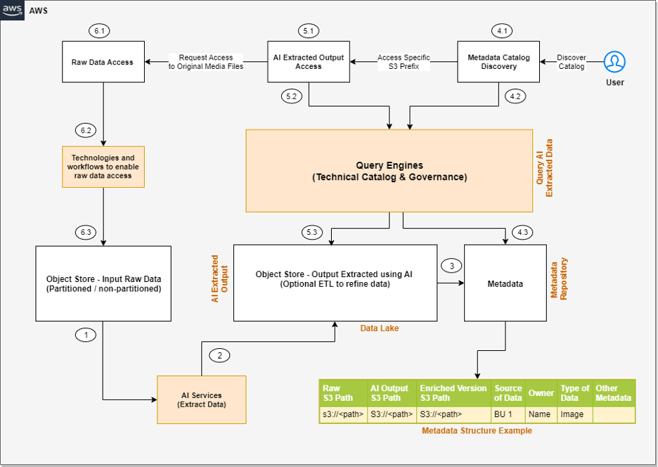
Unstructured Data Management - Block Level Architecture Diagram

The steps of the workflow are as follows:

  1. Integrated AI services extract data from the unstructured data.
  2. These services write the output to a data lake.
  3. A metadata layer helps build the relationship between the raw data and AI extracted output. When the data and metadata are available for end-users, we can break the user access pattern into additional steps.
  4. In the metadata catalog discovery step, we can use query engines to access the metadata for discovery and apply filters as per our analytics needs. Then we move to the next stage of accessing the actual data extracted from the raw unstructured data.
  5. The end-user accesses the output of the AI services and uses the query engines to query the structured data available in the data lake. We can optionally integrate additional tools that help control access and provide governance.
  6. There might be scenarios where, after accessing the AI extracted output, the end-user wants to access the original raw object (such as media files) for further analysis. Additionally, we need to make sure we have access control policies so the end-user has access only to the respective raw data they want to access.

Now that we understand the high-level architecture, let’s discuss what AWS services we can integrate in each step of the architecture to provide an end-to-end solution.

The following diagram is the enhanced version of our solution architecture, where we have integrated AWS services.

Unstructured Data Management - AWS Native Architecture

Let’s understand how these AWS services are integrated in detail. We have divided the steps into two broad user flows: data processing and metadata enrichment (Steps 1–3) and end-users accessing the data and metadata with fine-grained access control (Steps 4–6).

  1. Various AI services (which we discuss in the next section) extract data from the unstructured datasets.
  2. The output is written to an Amazon Simple Storage Service (Amazon S3) bucket (labeled Extracted JSON in the preceding diagram). Optionally, we can restructure the input raw objects for better partitioning, which can help while implementing fine-grained access control on the raw input data (labeled as the Partitioned bucket in the diagram).
  3. After the initial data extraction phase, we can apply additional transformations to enrich the datasets using AWS Glue. We also build an additional metadata layer, which maintains a relationship between the raw S3 object path, the AI extracted output path, the optional enriched version S3 path, and any other metadata that will help the end-user discover the data.
  4. In the metadata catalog discovery step, we use the AWS Glue Data Catalog as the technical catalog, Amazon Athena and Amazon Redshift Spectrum as query engines, AWS Lake Formation for fine-grained access control, and Amazon DataZone for additional governance.
  5. The AI extracted output is expected to be available as a delimited file or in JSON format. We can create an AWS Glue Data Catalog table for querying using Athena or Redshift Spectrum. Like the previous step, we can use Lake Formation policies for fine-grained access control.
  6. Lastly, the end-user accesses the raw unstructured data available in Amazon S3 for further analysis. We have proposed integrating Amazon S3 Access Points for access control at this layer. We explain this in detail later in this post.

Now let’s expand the following parts of the architecture to understand the implementation better:

  • Using AWS AI services to process unstructured data
  • Using S3 Access Points to integrate access control on raw S3 unstructured data

Process unstructured data with AWS AI services

As we discussed earlier, unstructured data can come in a variety of formats, such as text, audio, video, and images, and each type of data requires a different approach for extracting metadata. AWS AI services are designed to extract metadata from different types of unstructured data. The following are the most commonly used services for unstructured data processing:

  • Amazon Comprehend – This natural language processing (NLP) service uses ML to extract metadata from text data. It can analyze text in multiple languages, detect entities, extract key phrases, determine sentiment, and more. With Amazon Comprehend, you can easily gain insights from large volumes of text data such as extracting product entity, customer name, and sentiment from social media posts.
  • Amazon Transcribe – This speech-to-text service uses ML to convert speech to text and extract metadata from audio data. It can recognize multiple speakers, transcribe conversations, identify keywords, and more. With Amazon Transcribe, you can convert unstructured data such as customer support recordings into text and further derive insights from it.
  • Amazon Rekognition – This image and video analysis service uses ML to extract metadata from visual data. It can recognize objects, people, faces, and text, detect inappropriate content, and more. With Amazon Rekognition, you can easily analyze images and videos to gain insights such as identifying entity type (human or other) and identifying if the person is a known celebrity in an image.
  • Amazon Textract – You can use this ML service to extract metadata from scanned documents and images. It can extract text, tables, and forms from images, PDFs, and scanned documents. With Amazon Textract, you can digitize documents and extract data such as customer name, product name, product price, and date from an invoice.
  • Amazon SageMaker – This service enables you to build and deploy custom ML models for a wide range of use cases, including extracting metadata from unstructured data. With SageMaker, you can build custom models that are tailored to your specific needs, which can be particularly useful for extracting metadata from unstructured data that requires a high degree of accuracy or domain-specific knowledge.
  • Amazon Bedrock – This fully managed service offers a choice of high-performing foundation models (FMs) from leading AI companies like AI21 Labs, Anthropic, Cohere, Meta, Stability AI, and Amazon with a single API. It also offers a broad set of capabilities to build generative AI applications, simplifying development while maintaining privacy and security.

With these specialized AI services, you can efficiently extract metadata from unstructured data and use it for further analysis and insights. It’s important to note that each service has its own strengths and limitations, and choosing the right service for your specific use case is critical for achieving accurate and reliable results.

AWS AI services are available via various APIs, which enables you to integrate AI capabilities into your applications and workflows. AWS Step Functions is a serverless workflow service that allows you to coordinate and orchestrate multiple AWS services, including AI services, into a single workflow. This can be particularly useful when you need to process large amounts of unstructured data and perform multiple AI-related tasks, such as text analysis, image recognition, and NLP.

With Step Functions and AWS Lambda functions, you can create sophisticated workflows that include AI services and other AWS services. For instance, you can use Amazon S3 to store input data, invoke a Lambda function to trigger an Amazon Transcribe job to transcribe an audio file, and use the output to trigger an Amazon Comprehend analysis job to generate sentiment metadata for the transcribed text. This enables you to create complex, multi-step workflows that are straightforward to manage, scalable, and cost-effective.

The following is an example architecture that shows how Step Functions can help invoke AWS AI services using Lambda functions.
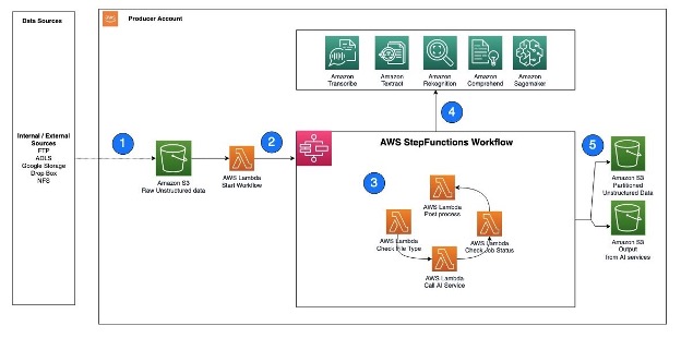
AWS AI Services - Lambda Event Workflow -Unstructured Data

The workflow steps are as follows:

  1. Unstructured data, such as text files, audio files, and video files, are ingested into the S3 raw bucket.
  2. A Lambda function is triggered to read the data from the S3 bucket and call Step Functions to orchestrate the workflow required to extract the metadata.
  3. The Step Functions workflow checks the type of file, calls the corresponding AWS AI service APIs, checks the job status, and performs any postprocessing required on the output.
  4. AWS AI services can be accessed via APIs and invoked as batch jobs. To extract metadata from different types of unstructured data, you can use multiple AI services in sequence, with each service processing the corresponding file type.
  5. After the Step Functions workflow completes the metadata extraction process and performs any required postprocessing, the resulting output is stored in an S3 bucket for cataloging.

Next, let’s understand how can we implement security or access control on both the extracted output as well as the raw input objects.

Implement access control on raw and processed data in Amazon S3

We just consider access controls for three types of data when managing unstructured data: the AI-extracted semi-structured output, the metadata, and the raw unstructured original files. When it comes to AI extracted output, it’s in JSON format and can be restricted via Lake Formation and Amazon DataZone. We recommend keeping the metadata (information that captures which unstructured datasets are already processed by the pipeline and available for analysis) open to your organization, which will enable metadata discovery across the organization.

To control access of raw unstructured data, you can integrate S3 Access Points and explore additional support in the future as AWS services evolve. S3 Access Points simplify data access for any AWS service or customer application that stores data in Amazon S3. Access points are named network endpoints that are attached to buckets that you can use to perform S3 object operations. Each access point has distinct permissions and network controls that Amazon S3 applies for any request that is made through that access point. Each access point enforces a customized access point policy that works in conjunction with the bucket policy that is attached to the underlying bucket. With S3 Access Points, you can create unique access control policies for each access point to easily control access to specific datasets within an S3 bucket. This works well in multi-tenant or shared bucket scenarios where users or teams are assigned to unique prefixes within one S3 bucket.

An access point can support a single user or application, or groups of users or applications within and across accounts, allowing separate management of each access point. Every access point is associated with a single bucket and contains a network origin control and a Block Public Access control. For example, you can create an access point with a network origin control that only permits storage access from your virtual private cloud (VPC), a logically isolated section of the AWS Cloud. You can also create an access point with the access point policy configured to only allow access to objects with a defined prefix or to objects with specific tags. You can also configure custom Block Public Access settings for each access point.

The following architecture provides an overview of how an end-user can get access to specific S3 objects by assuming a specific AWS Identity and Access Management (IAM) role. If you have a large number of S3 objects to control access, consider grouping the S3 objects, assigning them tags, and then defining access control by tags.
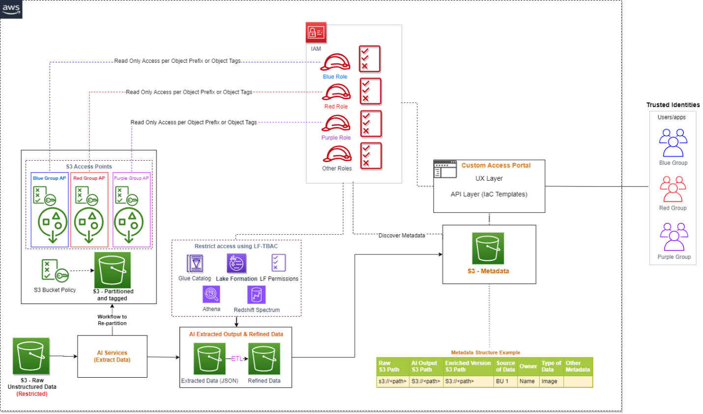
S3 Access Points - Unstructured Data Management - Access Control

If you are implementing a solution that integrates S3 data available in multiple AWS accounts, you can take advantage of cross-account support for S3 Access Points.

Conclusion

This post explained how you can use AWS AI services to extract readable data from unstructured datasets, build a metadata layer on top of them to allow data discovery, and build an access control mechanism on top of the raw S3 objects and extracted data using Lake Formation, Amazon DataZone, and S3 Access Points.

In addition to AWS AI services, you can also integrate large language models with vector databases to enable semantic or similarity search on top of unstructured datasets. To learn more about how to enable semantic search on unstructured data by integrating Amazon OpenSearch Service as a vector database, refer to Try semantic search with the Amazon OpenSearch Service vector engine.

As of writing this post, S3 Access Points is one of the best solutions to implement access control on raw S3 objects using tagging, but as AWS service features evolve in the future, you can explore alternative options as well.


About the Authors

Sakti Mishra is a Principal Solutions Architect at AWS, where he helps customers modernize their data architecture and define their end-to-end data strategy, including data security, accessibility, governance, and more. He is also the author of the book Simplify Big Data Analytics with Amazon EMR. Outside of work, Sakti enjoys learning new technologies, watching movies, and visiting places with family.

Bhavana Chirumamilla is a Senior Resident Architect at AWS with a strong passion for data and machine learning operations. She brings a wealth of experience and enthusiasm to help enterprises build effective data and ML strategies. In her spare time, Bhavana enjoys spending time with her family and engaging in various activities such as traveling, hiking, gardening, and watching documentaries.

Sheela Sonone is a Senior Resident Architect at AWS. She helps AWS customers make informed choices and trade-offs about accelerating their data, analytics, and AI/ML workloads and implementations. In her spare time, she enjoys spending time with her family—usually on tennis courts.

Daniel Bruno is a Principal Resident Architect at AWS. He had been building analytics and machine learning solutions for over 20 years and splits his time helping customers build data science programs and designing impactful ML products.

Implement a CDC-based UPSERT in a data lake using Apache Iceberg and AWS Glue

Post Syndicated from Sakti Mishra original https://aws.amazon.com/blogs/big-data/implement-a-cdc-based-upsert-in-a-data-lake-using-apache-iceberg-and-aws-glue/

As the implementation of data lakes and modern data architecture increases, customers’ expectations around its features also increase, which include ACID transaction, UPSERT, time travel, schema evolution, auto compaction, and many more. By default, Amazon Simple Storage Service (Amazon S3) objects are immutable, which means you can’t update records in your data lake because it supports append-only transactions. But there are use cases where you might be receiving incremental updates with change data capture (CDC) from your source systems, and you might need to update existing data in Amazon S3 to have a golden copy. Previously, you had to overwrite the complete S3 object or folders, but with the evolution of frameworks such as Apache Hudi, Apache Iceberg, Delta Lake, and governed tables in AWS Lake Formation, you can get database-like UPSERT features in Amazon S3.

Apache Hudi integration is already supported with AWS analytics services, and recently AWS Glue, Amazon EMR, and Amazon Athena announced support for Apache Iceberg. Apache Iceberg is an open table format originally developed at Netflix, which got open-sourced as an Apache project in 2018 and graduated from incubator mid-2020. It’s designed to support ACID transactions and UPSERT on petabyte-scale data lakes, and is getting popular because of its flexible SQL syntax for CDC-based MERGE, full schema evolution, and hidden partitioning features.

In this post, we walk you through a solution to implement CDC-based UPSERT or MERGE in an S3 data lake using Apache Iceberg and AWS Glue.

Configure Apache Iceberg with AWS Glue

You can integrate Apache Iceberg JARs into AWS Glue through its AWS Marketplace connector. The connector supports AWS Glue versions 1.0, 2.0, and 3.0, and is free to use. Configuring this connector is as easy as clicking few buttons on the user interface.

The following steps guide you through the setup process:

  1. Navigate to the AWS Marketplace connector page.
  2. Choose Continue to Subscribe and then Accept Terms.
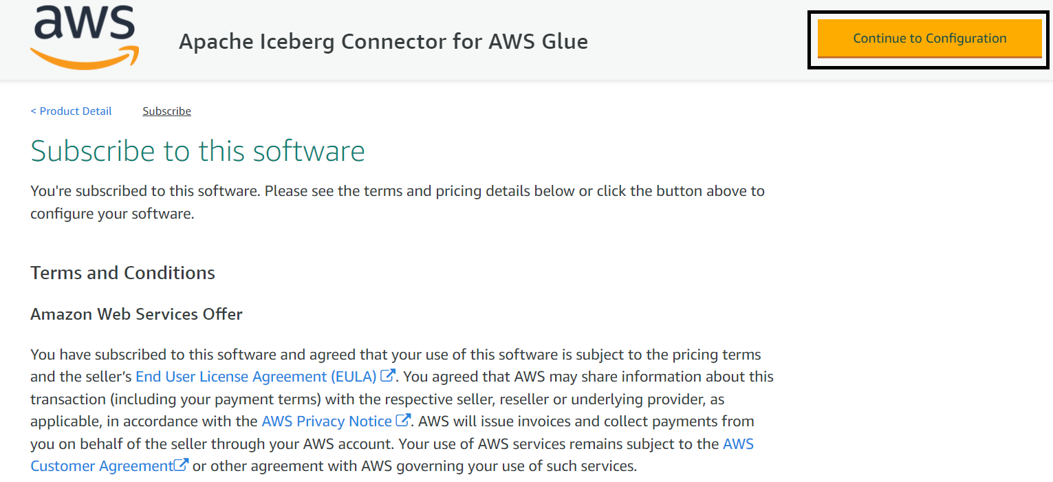
  3. Choose Continue to Configuration.
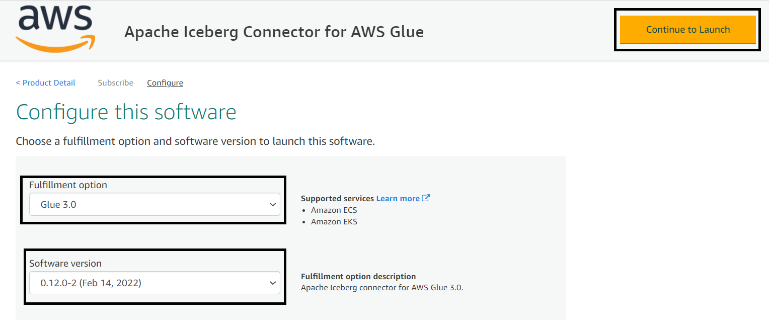
  4. Choose the AWS Glue version and software version.
  5. Choose Continue to Launch.
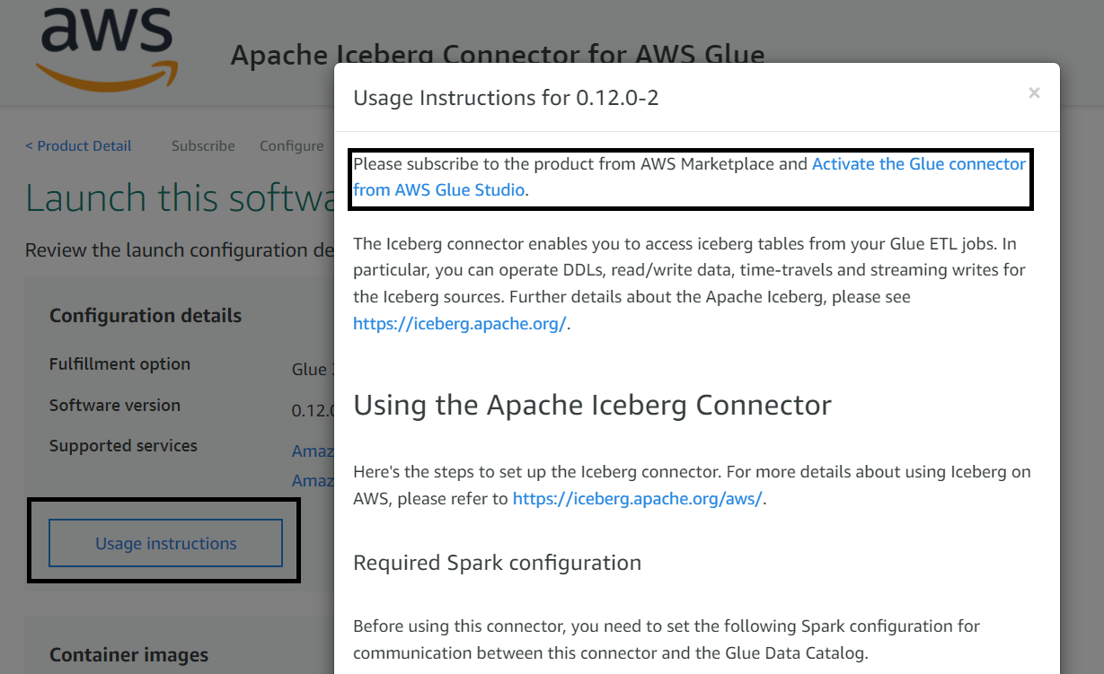
  6. Choose Usage Instruction, which opens a page that has a link to activate the connector.
  7. Create a connection by providing a name and choosing Create connection and activate connector.

You can confirm your new connection on the AWS Glue Studio Connectors page.

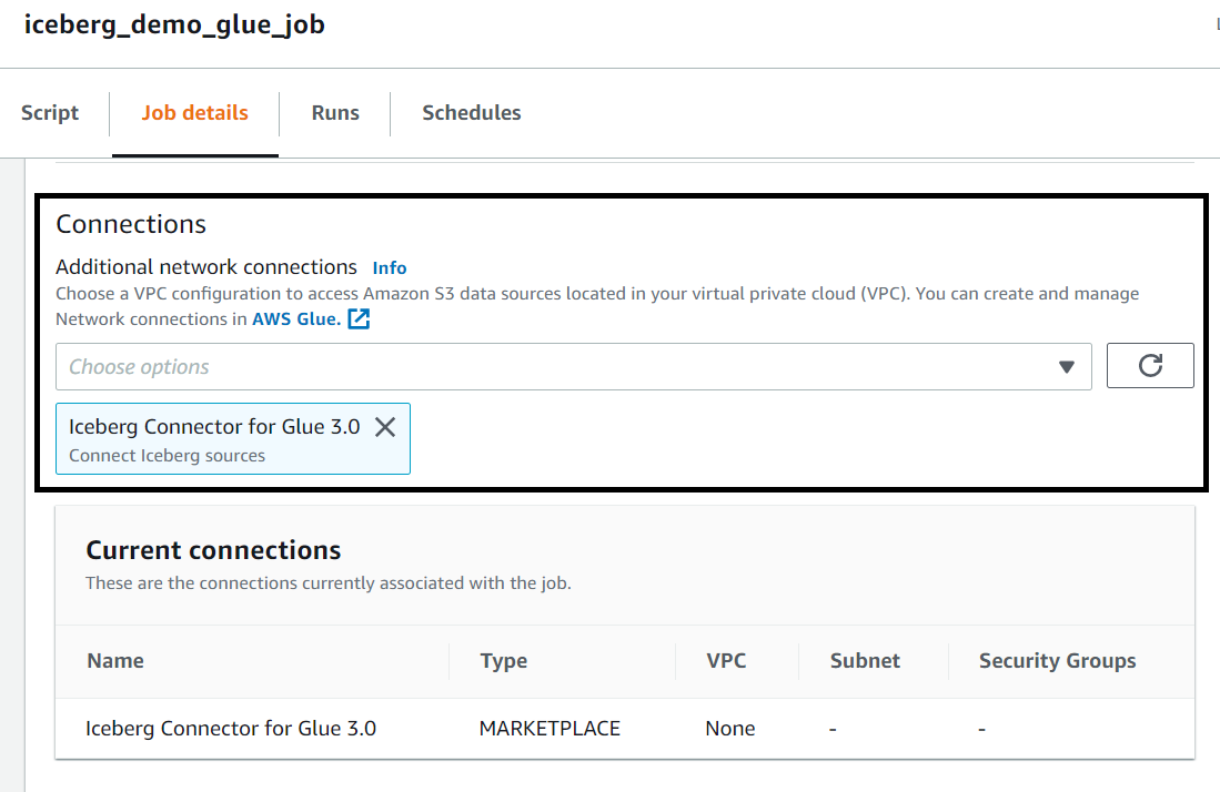
To use this connector, when you create an AWS Glue job, make sure you add this connector to your job. Later in the implementation steps, when you create an AWS Glue job, we show how to use the connector you just configured.

Solution overview

Let’s assume you have a relational database that has product inventory data, and you want to move it into an S3 data lake on a continuous basis, so that your downstream applications or consumers can use it for analytics. After your initial data movement to Amazon S3, you’re supposed to receive incremental updates from the source database as CSV files using AWS DMS or equivalent tools, where each record has an additional column to represent an insert, update, or delete operation. While processing the incremental CDC data, one of the primary requirements you have is merging the CDC data in the data lake and providing the capability to query previous versions of the data.

To solve this use case, we present the following simple architecture that integrates Amazon S3 for the data lake, AWS Glue with the Apache Iceberg connector for ETL (extract, transform, and load), and Athena for querying the data using standard SQL. Athena helps in querying the latest product inventory data from the Iceberg table’s latest snapshot, and Iceberg’s time travel feature helps in identifying a product’s price at any previous date.

The following diagram illustrates the solution architecture.

The solution workflow consists of the following steps:

  • Data ingestion:
    • Steps 1.1 and 1.2 use AWS Database Migration Service (AWS DMS), which connects to the source database and moves incremental data (CDC) to Amazon S3 in CSV format.
    • Steps 1.3 and 1.4 consist of the AWS Glue PySpark job, which reads incremental data from the S3 input bucket, performs deduplication of the records, and then invokes Apache Iceberg’s MERGE statements to merge the data with the target UPSERT S3 bucket.
  • Data access:
    • Steps 2.1 and 2.2 represent Athena integration to query data from the Iceberg table using standard SQL and validate the time travel feature of Iceberg.
  • Data Catalog:
    • The AWS Glue Data Catalog is treated as a centralized catalog, which is used by AWS Glue and Athena. An AWS Glue crawler is integrated on top of S3 buckets to automatically detect the schema.

We have referenced AWS DMS as part of the architecture, but while showcasing the solution steps, we assume that the AWS DMS output is already available in Amazon S3, and focus on processing the data using AWS Glue and Apache Iceberg.

To demo the implementation steps, we use sample product inventory data that has the following attributes:

  • op – Represents the operation on the source record. This shows values I to represent insert operations, U to represent updates, and D to represent deletes. You need to make sure this attribute is included in your CDC incremental data before it gets written to Amazon S3. AWS DMS enables you to include this attribute, but if you’re using other mechanisms to move data, make sure you capture this attribute, so that your ETL logic can take appropriate action while merging it.
  • product_id – This is the primary key column in the source database’s products table.
  • category – This column represents the product’s category, such as Electronics or Cosmetics.
  • product_name – This is the name of the product.
  • quantity_available – This is the quantity available in the inventory for a product. When we showcase the incremental data for UPSERT or MERGE, we reduce the quantity available for the product to showcase the functionality.
  • last_update_time – This is the time when the product record was updated at the source database.

If you’re using AWS DMS to move data from your relational database to Amazon S3, then by default AWS DMS includes the op attribute for incremental CDC data, but it’s not included by default for the initial load. If you’re using CSV as your target file format, you can include IncludeOpForFullLoad as true in your S3 target endpoint setting of AWS DMS to have the op attribute included in your initial full load file. To learn more about the Amazon S3 settings in AWS DMS, refer to S3Settings.

To implement the solution, we create AWS resources such as an S3 bucket and an AWS Glue job, and integrate the Iceberg code for processing. Before we run the AWS Glue job, we have to upload the sample CSV files to the input bucket and process it with AWS Glue PySpark code for the output.

Prerequisites

Before getting started on the implementation, make sure you have the required permissions to perform the following in your AWS account:

  • Create AWS Identity and Access Management (IAM) roles as needed
  • Read or write to an S3 bucket
  • Create and run AWS Glue crawlers and jobs
  • Manage a database, table, and workgroups, and run queries in Athena

For this post, we use the us-east-1 Region, but you can integrate it in your preferred Region if the AWS services included in the architecture are available in that Region.

Now let’s dive into the implementation steps.

Create an S3 bucket for input and output

To create an S3 bucket, complete the following steps:

  1. On the Amazon S3 console, choose Buckets in the navigation pane.
  2. Choose Create bucket.
  3. Specify the bucket name as glue-iceberg-demo, and leave the remaining fields as default.
    S3 bucket names are globally unique. While implementing the solution, you may get an error saying the bucket name already exists. Make sure to provide a unique name and use the same name while implementing the rest of the implementation steps. Formatting the bucket name as <Bucket-Name>-${AWS_ACCOUNT_ID}-${AWS_REGION_CODE} might help you get a unique name.
  4. Choose Create bucket.
  5. On the bucket details page, choose Create folder.
  6. Create two subfolders: raw-csv-input and iceberg-output.
  7. Upload the LOAD00000001.csv file into the raw-csv-input folder of the bucket.

The following screenshot provides a sample of the input dataset.

Create input and output tables using Athena

To create input and output Iceberg tables in the AWS Glue Data Catalog, open the Athena console and run the following queries in sequence:

-- Create database for the demo
CREATE DATABASE iceberg_demo;
-- Create external table in input CSV files. Replace the S3 path with your bucket name
CREATE EXTERNAL TABLE iceberg_demo.raw_csv_input(
  op string, 
  product_id bigint, 
  category string, 
  product_name string, 
  quantity_available bigint, 
  last_update_time string)
ROW FORMAT DELIMITED FIELDS TERMINATED BY ',' 
STORED AS INPUTFORMAT 'org.apache.hadoop.mapred.TextInputFormat' 
OUTPUTFORMAT 'org.apache.hadoop.hive.ql.io.HiveIgnoreKeyTextOutputFormat'
LOCATION 's3://glue-iceberg-demo/raw-csv-input/'
TBLPROPERTIES (
  'areColumnsQuoted'='false', 
  'classification'='csv', 
  'columnsOrdered'='true', 
  'compressionType'='none', 
  'delimiter'=',', 
  'typeOfData'='file');
-- Create output Iceberg table with partitioning. Replace the S3 bucket name with your bucket name
CREATE TABLE iceberg_demo.iceberg_output (
  product_id bigint,
  category string,
  product_name string,
  quantity_available bigint,
  last_update_time timestamp) 
PARTITIONED BY (category, bucket(16,product_id)) 
LOCATION 's3://glue-iceberg-demo/iceberg-output/' 
TBLPROPERTIES (
  'table_type'='ICEBERG',
  'format'='parquet',
  'write_target_data_file_size_bytes'='536870912' 
)
-- Validate the input data
SELECT * FROM iceberg_demo.raw_csv_input;

Alternatively, you can integrate an AWS Glue crawler on top of the input to create the table. Next, let’s create the AWS Glue PySpark job to process the input data.

Create the AWS Glue job

Complete the following steps to create an AWS Glue job:

  1. On the AWS Glue console, choose Jobs in the navigation pane.
  2. Choose Create job.
  3. Select Spark script editor.
  4. For Options, select Create a new script with boilerplate code.
  5. Choose Create.
  6. Replace the script with the following script:
    import sys
    from awsglue.transforms import *
    from awsglue.utils import getResolvedOptions
    from pyspark.context import SparkContext
    from awsglue.context import GlueContext
    from awsglue.job import Job
    
    from pyspark.sql.functions import *
    from awsglue.dynamicframe import DynamicFrame
    
    from pyspark.sql.window import Window
    from pyspark.sql.functions import rank, max
    
    from pyspark.conf import SparkConf
    
    args = getResolvedOptions(sys.argv, ['JOB_NAME', 'iceberg_job_catalog_warehouse'])
    conf = SparkConf()
    
    ## Please make sure to pass runtime argument --iceberg_job_catalog_warehouse with value as the S3 path 
    conf.set("spark.sql.catalog.job_catalog.warehouse", args['iceberg_job_catalog_warehouse'])
    conf.set("spark.sql.catalog.job_catalog", "org.apache.iceberg.spark.SparkCatalog")
    conf.set("spark.sql.catalog.job_catalog.catalog-impl", "org.apache.iceberg.aws.glue.GlueCatalog")
    conf.set("spark.sql.catalog.job_catalog.io-impl", "org.apache.iceberg.aws.s3.S3FileIO")
    conf.set("spark.sql.extensions", "org.apache.iceberg.spark.extensions.IcebergSparkSessionExtensions")
    conf.set("spark.sql.sources.partitionOverwriteMode", "dynamic")
    conf.set("spark.sql.iceberg.handle-timestamp-without-timezone","true")
    
    sc = SparkContext(conf=conf)
    glueContext = GlueContext(sc)
    spark = glueContext.spark_session
    job = Job(glueContext)
    job.init(args["JOB_NAME"], args)
    
    ## Read Input Table
    IncrementalInputDyF = glueContext.create_dynamic_frame.from_catalog(database = "iceberg_demo", table_name = "raw_csv_input", transformation_ctx = "IncrementalInputDyF")
    IncrementalInputDF = IncrementalInputDyF.toDF()
    
    if not IncrementalInputDF.rdd.isEmpty():
        ## Apply De-duplication logic on input data, to pickup latest record based on timestamp and operation 
        IDWindowDF = Window.partitionBy(IncrementalInputDF.product_id).orderBy(IncrementalInputDF.last_update_time).rangeBetween(-sys.maxsize, sys.maxsize)
                      
        # Add new columns to capture first and last OP value and what is the latest timestamp
        inputDFWithTS= IncrementalInputDF.withColumn("max_op_date",max(IncrementalInputDF.last_update_time).over(IDWindowDF))
        
        # Filter out new records that are inserted, then select latest record from existing records and merge both to get deduplicated output 
        NewInsertsDF = inputDFWithTS.filter("last_update_time=max_op_date").filter("op='I'")
        UpdateDeleteDf = inputDFWithTS.filter("last_update_time=max_op_date").filter("op IN ('U','D')")
        finalInputDF = NewInsertsDF.unionAll(UpdateDeleteDf)
    
        # Register the deduplicated input as temporary table to use in Iceberg Spark SQL statements
        finalInputDF.createOrReplaceTempView("incremental_input_data")
        finalInputDF.show()
        
        ## Perform merge operation on incremental input data with MERGE INTO. This section of the code uses Spark SQL to showcase the expressive SQL approach of Iceberg to perform a Merge operation
        IcebergMergeOutputDF = spark.sql("""
        MERGE INTO job_catalog.iceberg_demo.iceberg_output t
        USING (SELECT op, product_id, category, product_name, quantity_available, to_timestamp(last_update_time) as last_update_time FROM incremental_input_data) s
        ON t.product_id = s.product_id
        WHEN MATCHED AND s.op = 'D' THEN DELETE
        WHEN MATCHED THEN UPDATE SET t.quantity_available = s.quantity_available, t.last_update_time = s.last_update_time 
        WHEN NOT MATCHED THEN INSERT (product_id, category, product_name, quantity_available, last_update_time) VALUES (s.product_id, s.category, s.product_name, s.quantity_available, s.last_update_time)
        """)
    
        job.commit()

  7. On the Job details tab, specify the job name.
  8. For IAM Role, assign an IAM role that has the required permissions to run an AWS Glue job and read and write to the S3 bucket.
  9. For Glue version, choose Glue 3.0.
  10. For Language, choose Python 3.
  11. Make sure Job bookmark has default value of Enable.
  12. Under Connections, choose the Iceberg connector.
  13. Under Job parameters, specify Key as --iceberg_job_catalog_warehouse and Value as your S3 path (e.g. s3://<bucket-name>/<iceberg-warehouse-path>).
  14. Choose Save and then Run, which should write the input data to the Iceberg table with a MERGE statement.

Because the target table is empty in the first run, the Iceberg MERGE statement runs an INSERT statement for all records.

Query the Iceberg table using Athena

After you have successfully run the AWS Glue job, you can validate the output in Athena with the following SQL query:

SELECT * FROM iceberg_demo.iceberg_output limit 10;

The output of the query should match the input, with one difference: The Iceberg output table doesn’t have the op column.

Upload incremental (CDC) data for further processing

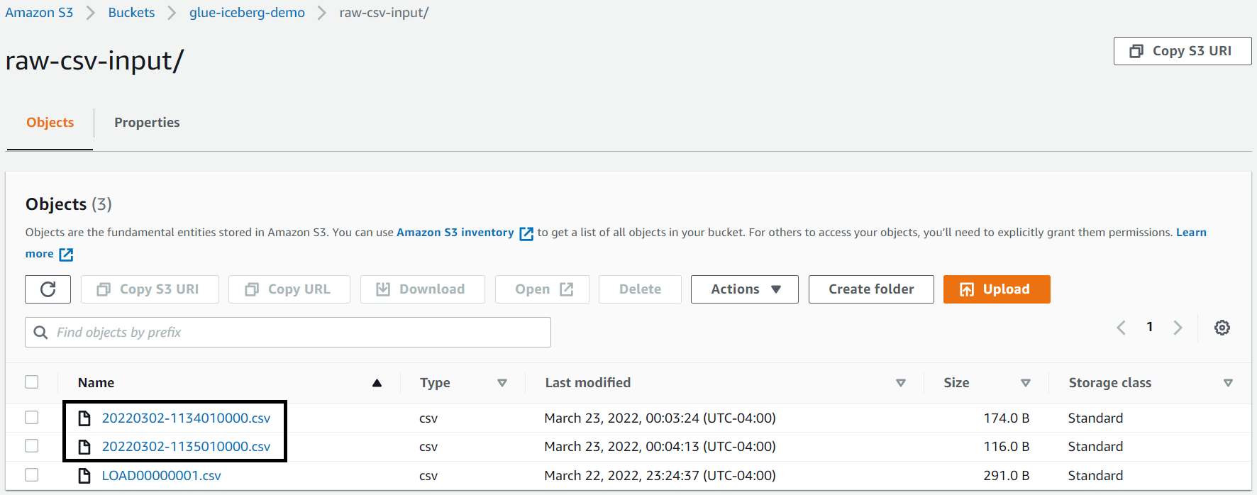
After we process the initial full load file, let’s upload the following two incremental files, which include insert, update, and delete records for a few products.
The following is a snapshot of first incremental file (20220302-1134010000.csv).

The following is a snapshot of the second incremental file (20220302-1135010000.csv), which shows that record 102 has another update transaction before the next ETL job processing.

After you upload both incremental files, you should see them in the S3 bucket.

Run the AWS Glue job again to process incremental files

Because we enabled bookmarks on the AWS Glue job, the next job picks up only the two new incremental files and performs a merge operation on the Iceberg table.

To run the job again, complete the following steps:

  • On the AWS Glue console, choose Jobs in the navigation pane.
  • Select the job and choose Run.

As explained earlier, the PySpark script is expected to deduplicate the input data before merging to the target Iceberg table, which means it only picks up the latest record of the 102 product.

For this post, we run the job manually, but you can configure your AWS Glue jobs to run as part of an AWS Glue workflow or via AWS Step Functions (for more information, see Manage AWS Glue Jobs with Step Functions).

Query the Iceberg table using Athena, after incremental data processing

After incremental data processing is complete, you can run the same SELECT statement again and validate that the quantity value is updated for record 102 and product record 103 is deleted.

The following screenshot shows the output.

Query the previous version of data with Iceberg’s time travel feature

You can run the following SQL query in Athena that uses the AS OF TIME statement of Iceberg to query the previous version of the data:

-SELECT * FROM iceberg_demo.iceberg_output FOR SYSTEM_TIME AS OF TIMESTAMP '2022-03-23 18:56:00'

The following screenshot shows the output. As you can see, the quantity value of product ID 102 is 30, which was available during the initial load.

Note that you have to change the AS OF TIMESTAMP value based on your runtime.

This concludes the implementation steps.

Considerations

The following are a few considerations you should keep in mind while integrating Apache Iceberg with AWS Glue:

  • Athena support for Iceberg became generally available recently, so make sure you review the considerations and limitations of using this feature.
  • AWS Glue provides DynamicFrame APIs to read from different source systems and write to different targets. For this post, we integrated Spark DataFrame instead of AWS Glue DynamicFrame because Iceberg’s MERGE statements aren’t supported with AWS Glue DynamicFrame APIs.
    To learn more about AWS integration, refer to Iceberg AWS Integrations.

Conclusion

This post explains how you can use the Apache Iceberg framework with AWS Glue to implement UPSERT on an S3 data lake. It provides an overview of Apache Iceberg, its features and integration approaches, and explains how you can implement it through a step-by-step guide.

I hope this gives you a great starting point for using Apache Iceberg with AWS analytics services and that you can build on top of it to implement your solution.

Appendix: AWS Glue DynamicFrame sample code to interact with Iceberg tables

  • The following code sample demonstrates how you can integrate the DynamicFrame method to read from an Iceberg table:
IcebergDyF = (
    glueContext.create_dynamic_frame.from_options(
        connection_type="marketplace.spark",
        connection_options={
            "path": "job_catalog.iceberg_demo.iceberg_output",
            "connectionName": "Iceberg Connector for Glue 3.0",
        },
        transformation_ctx="IcebergDyF",
    )
)

## Optionally, convert to Spark DataFrame if you plan to leverage Iceberg’s SQL based MERGE statements
InputIcebergDF = IcebergDyF.toDF()
  • The following sample code shows how you can integrate the DynamicFrame method to write to an Iceberg table for append-only mode:
## Use the following 2 lines to convert Spark DataFrame to DynamicFrame, if you plan to leverage DynamicFrame API to write to final target
from awsglue.dynamicframe import DynamicFrame 
finalDyF = DynamicFrame.fromDF(InputIcebergDF,glueContext,"finalDyF")

WriteIceberg = glueContext.write_dynamic_frame.from_options(
    frame= finalDyF,
    connection_type="marketplace.spark",
    connection_options={
        "path": "job_catalog.iceberg_demo.iceberg_output",
        "connectionName": "Iceberg Connector for Glue 3.0",
    },
    format="parquet",
    transformation_ctx="WriteIcebergDyF",
)

About the Author

Sakti Mishra is a Principal Data Lab Solution Architect at AWS, where he helps customers modernize their data architecture and help define end to end data strategy including data security, accessibility, governance, and more. He is also the author of the book Simplify Big Data Analytics with Amazon EMR. Outside of work, Sakti enjoys learning new technologies, watching movies, and visiting places with family.

Orchestrating an AWS Glue DataBrew job and Amazon Athena query with AWS Step Functions

Post Syndicated from Sakti Mishra original https://aws.amazon.com/blogs/big-data/orchestrating-an-aws-glue-databrew-job-and-amazon-athena-query-with-aws-step-functions/

As the industry grows with more data volume, big data analytics is becoming a common requirement in data analytics and machine learning (ML) use cases. Also, as we start building complex data engineering or data analytics pipelines, we look for a simpler orchestration mechanism with graphical user interface-based ETL (extract, transform, load) tools.

Recently, AWS announced the general availability of AWS Glue DataBrew, a new visual data preparation tool that helps you clean and normalize data without writing code. This reduces the time it takes to prepare data for analytics and ML by up to 80% compared to traditional approaches to data preparation.

Regarding orchestration or workflow management, AWS provides AWS Step Functions, a serverless function orchestrator that makes it easy to build a workflow by integrating different AWS services like AWS Lambda, Amazon Simple Notification Service (Amazon SNS), AWS Glue, and more. With its built-in operational controls, Step Functions manages sequencing, error handling, retry logic, and states, removing a significant operational burden from your team.

Today, we’re launching Step Functions support for DataBrew, which means you can now invoke DataBrew jobs in your Step Functions workflow to build an end-to-end ETL pipeline. Recently, Step Functions also started supporting Amazon Athena integration, which means that you can submit SQL queries to the Athena engine through a Step Functions state.

In this post, we walk through a solution where we integrate a DataBrew job for data preparation, invoke a series of Athena queries for data refresh, and integrate Amazon QuickSight for business reporting. The whole solution is orchestrated through Step Functions and is invoked through Amazon EventBridge.

Use case overview

For our use case, we use two public datasets. The first dataset is a sales pipeline dataset, which contains a list of over 20,000 sales opportunity records for a fictitious business. Each record has fields that specify the following:

  • A date, potentially when an opportunity was identified
  • The salesperson’s name
  • A market segment to which the opportunity belongs
  • Forecasted monthly revenue

The second dataset is an online marketing metrics dataset. This dataset contains records of marketing metrics, aggregated by day. The metrics describe user engagement across various channels, such as websites, mobile, and social media, plus other marketing metrics. The two datasets are unrelated, but for the purpose of this post, we assume that they’re related.

For our use case, these sales and marketing CSV files are maintained by your organization’s Marketing team, which uploads the updated full CSV file to Amazon Simple Storage Service (Amazon S3) every month. The aggregated output data is created through a series of data preparation steps, and the business team uses the output data to create business intelligence (BI) reports.

Architecture overview

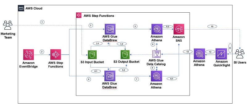
To automate the complete process, we use the following architecture, which integrates Step Functions for orchestration, DataBrew for data preparation, Athena for data analysis with standard SQL, and QuickSight for business reporting. In addition, we use Amazon SNS for sending notifications to users, and EventBridge is integrated to schedule running the Step Functions workflow.

We use Amazon SNS for sending notifications to users, and EventBridge is integrated to schedule running the Step Functions workflow.

The workflow includes the following steps:

  • Step 1 – The Marketing team uploads the full CSV file to an S3 input bucket every month.
  • Step 2 – An EventBridge rule, scheduled to run every month, triggers the Step Functions state machine.
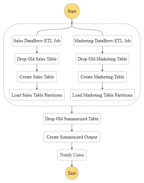
  • Steps 3 and 4 – We receive two separate datasets (sales data and marketing data), so Step Functions triggers two parallel DataBrew jobs, which create additional year, month, and day columns from the existing date field and uses those three columns for partitioning. The jobs write the final output to our S3 output bucket.
  • Steps 5, 6, 7, 8 – After the output data is written, we can create external tables on top of it with Athena create table statements and then load partitions with MCSK REPAIR commands. After the AWS Glue Data Catalog tables are created for sales and marketing, we run an additional query through Athena, which merges these two tables by year and month to create another table with aggregated output.
  • Steps 9 and 10 – As the last step of the Step Functions workflow, we send a notification to end-users through Amazon SNS to notify them that the data refresh job completed successfully.
  • Steps 11, 12, 13 – After the aggregated table data is refreshed, business users can use QuickSight for BI reporting, which fetches data through Athena. Data analysts can also use Athena to analyze the complete refreshed dataset.

Prerequisites

Before beginning this tutorial, make sure you have the required permissions to create the resources required as part of the solution.

Additionally, create the S3 input and output buckets with the required subfolders to capture the sales and marketing data, and upload the input data into their respective folders.

Creating a DataBrew project

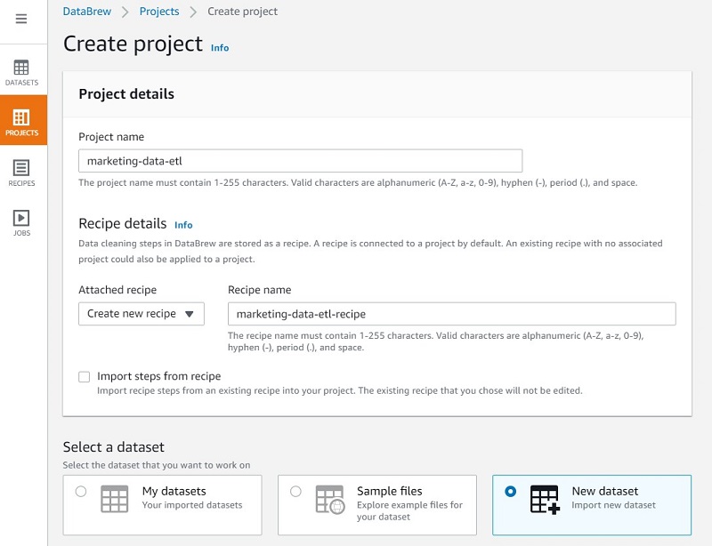
To create a DataBrew project for the marketing data, complete the following steps:

  1. On the DataBrew console, choose Projects.
  2. Choose Create a project.
  3. For Project name, enter a name (for this post, marketing-data-etl).
  4. For Select a dataset, select New dataset.

For Select a dataset, select New dataset.

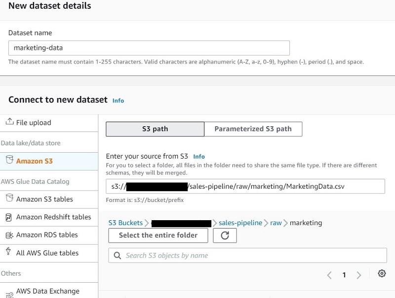
  1. For Enter your source from S3, enter the S3 path of the marketing input CSV.

For Enter your source from S3, enter the S3 path of the marketing input CSV.

  1. Under Permissions, for Role name, choose an AWS Identity and Access Management (IAM) role that allows DataBrew to read from your Amazon S3 input location.

You can choose a role if you already created one, or create a new one. Please read here for steps to create the IAM role.

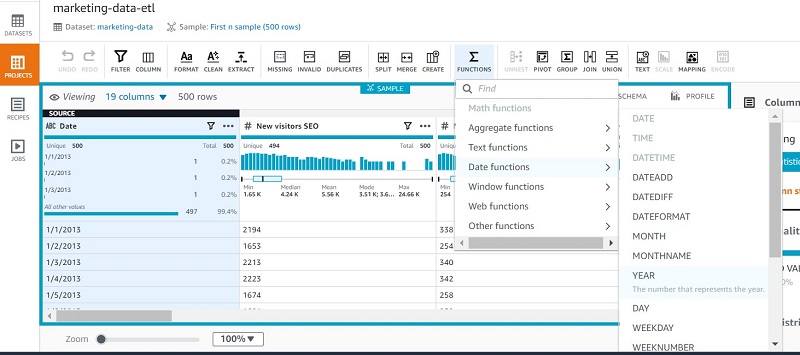
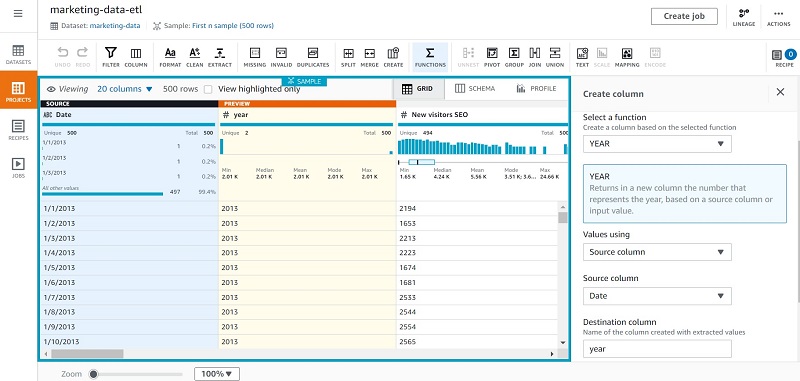
  1. After the dataset is loaded, on the Functions menu, choose Date functions.
  2. Choose YEAR.

Choose YEAR.

  1. Apply the year function on the date column to create a new column called year.

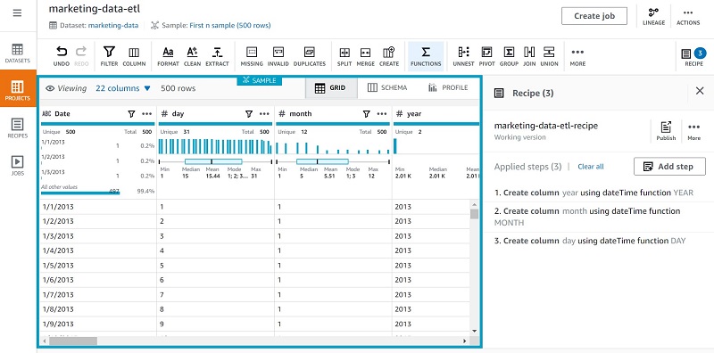
  1. Repeat these steps to create month and day columns.

Repeat these steps to create month and day columns.

For our use case, we created a few new columns that we plan to use for partitioning, but you can integrate additional transformations as needed.

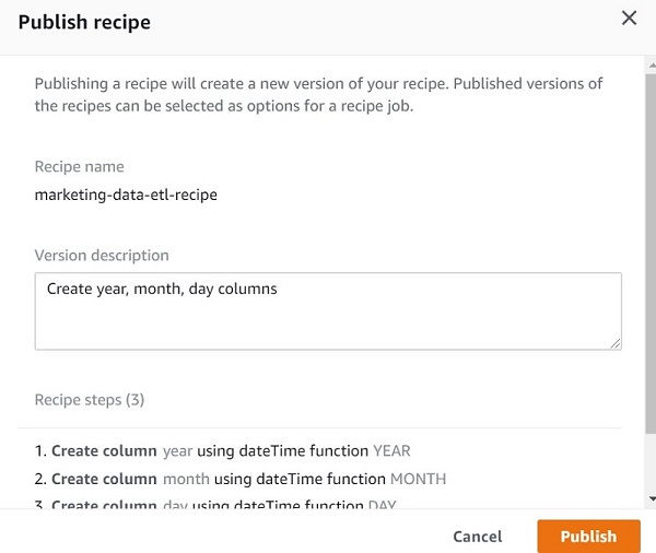
  1. After you have finished applying all your transformations, choose Publish on the recipe.
  2. Provide a description of the recipe version and choose Publish.

Creating a DataBrew job

Now that our recipe is ready, we can create a job for it, which gets invoked through our Step Functions state machine.

  1. On the DataBrew console, choose Jobs.
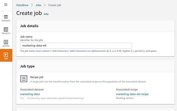
  2. Choose Create a job.
  3. For Job name¸ enter a name (for example, marketing-data-etl).

Your recipe is already linked to the job.

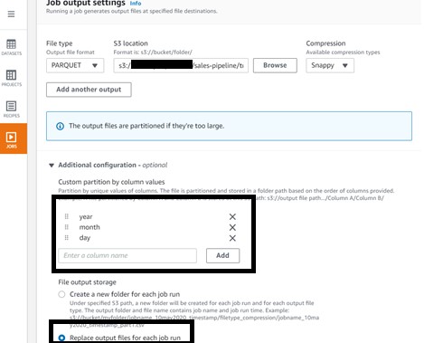
  1. Under Job output settings¸ for File type, choose your final storage format (for this post, we choose PARQUET).
  2. For S3 location, enter your final S3 output bucket path.
  3. For Compression, choose the compression type you want to apply (for this post, we choose Snappy).
  4. Under Additional configurations, for Custom partition by column values, choose year, month, and day.
  5. For File output storage, select Replace output files for each job run.

We choose this option because our use case is to do a full refresh.

We choose this option because our use case is to do a full refresh.

  1. Under Permissions, for Role name¸ choose your IAM role.
  2. Choose Create job.

We choose this because we don’t want to run it now; we plan to invoke it through Step Functions.

We choose this because we don’t want to run it now; we plan to invoke it through Step Functions.

  1. When your marketing job is ready, repeat the same steps for your sales data, using the sales data output file location as needed.

Creating a Step Functions state machine

We’re now ready to create a Step Functions state machine for the complete flow.

  1. On the Step Functions console, choose Create state machine.
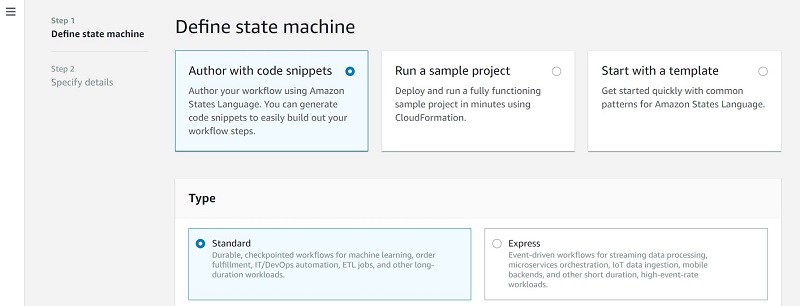
  2. For Define state machine¸ select Author with code snippets.
  3. For Type, choose Standard.

For Type, choose Standard.

In the Definition section, Step Functions provides a list of service actions that you can use to automatically generate a code snippet for your state machine’s state. The following screenshot shows that we have options for Athena and DataBrew, among others.
  1. For Generate code snippet, choose AWS Glue DataBrew: Start a job run.
4. For Generate code snippet, choose AWS Glue DataBrew: Start a job run.

  1. For Job name, choose Select job name from a list and choose your DataBrew job.

The JSON snippet appears in the Preview pane.

  1. Select Wait for DataBrew job runs to complete.
  2. Choose Copy to clipboard.

Choose Copy to clipboard.

  1. Integrate the code into the final state machine JSON code:
    {
       "Comment":"Monthly Refresh of Sales Marketing Data",
       "StartAt":"Refresh Sales Marketing Data",
       "States":{
          "Refresh Sales Marketing Data":{
             "Type":"Parallel",
             "Branches":[
                {
                   "StartAt":"Sales DataBrew ETL Job",
                   "States":{
                      "Sales DataBrew ETL Job":{
                         "Type":"Task",
                         "Resource":"arn:aws:states:::databrew:startJobRun.sync",
                         "Parameters":{
                            "Name":"sales-data"
                         },
                         "Next":"Drop Old Sales Table"
                      },
                      "Drop Old Sales Table":{
                         "Type":"Task",
                         "Resource":"arn:aws:states:::athena:startQueryExecution.sync",
                         "Parameters":{
                            "QueryString":"DROP TABLE IF EXISTS sales_data_output",
                            "WorkGroup":"primary",
                            "ResultConfiguration":{
                               "OutputLocation":"s3://<your-aws-athena-query-results-bucket-path>/"
                            }
                         },
                         "Next":"Create Sales Table"
                      },
                      "Create Sales Table":{
                         "Type":"Task",
                         "Resource":"arn:aws:states:::athena:startQueryExecution.sync",
                         "Parameters":{
                            "QueryString":"CREATE EXTERNAL TABLE `sales_data_output`(`date` string, `salesperson` string, `lead_name` string, `segment` string, `region` string, `target_close` string, `forecasted_monthly_revenue` int,   `opportunity_stage` string, `weighted_revenue` int, `closed_opportunity` boolean, `active_opportunity` boolean, `latest_status_entry` boolean) PARTITIONED BY (`year` string,`month` string, `day` string) ROW FORMAT SERDE 'org.apache.hadoop.hive.ql.io.parquet.serde.ParquetHiveSerDe' STORED AS INPUTFORMAT   'org.apache.hadoop.hive.ql.io.parquet.MapredParquetInputFormat' OUTPUTFORMAT   'org.apache.hadoop.hive.ql.io.parquet.MapredParquetOutputFormat' LOCATION  's3://<your-bucket-name>/sales-pipeline/transformed/sales/' TBLPROPERTIES ('classification'='parquet', 'compressionType'='none', 'typeOfData'='file')",
                            "WorkGroup":"primary",
                            "ResultConfiguration":{
                               "OutputLocation":"s3://<your-aws-athena-query-results-bucket-path>/"
                            }
                         },
                         "Next":"Load Sales Table Partitions"
                      },
                      "Load Sales Table Partitions":{
                         "Type":"Task",
                         "Resource":"arn:aws:states:::athena:startQueryExecution.sync",
                         "Parameters":{
                            "QueryString":"MSCK REPAIR TABLE sales_data_output",
                            "WorkGroup":"primary",
                            "ResultConfiguration":{
                               "OutputLocation":"s3://<your-aws-athena-query-results-bucket-path>/"
                            }
                         },
                         "End":true
                      }
                   }
                },
                {
                   "StartAt":"Marketing DataBrew ETL Job",
                   "States":{
                      "Marketing DataBrew ETL Job":{
                         "Type":"Task",
                         "Resource":"arn:aws:states:::databrew:startJobRun.sync",
                         "Parameters":{
                            "Name":"marketing-data-etl"
                         },
                         "Next":"Drop Old Marketing Table"
                      },
                      "Drop Old Marketing Table":{
                         "Type":"Task",
                         "Resource":"arn:aws:states:::athena:startQueryExecution.sync",
                         "Parameters":{
                            "QueryString":"DROP TABLE IF EXISTS marketing_data_output",
                            "WorkGroup":"primary",
                            "ResultConfiguration":{
                               "OutputLocation":"s3://<your-aws-athena-query-results-bucket-path>/"
                            }
                         },
                         "Next":"Create Marketing Table"
                      },
                      "Create Marketing Table":{
                         "Type":"Task",
                         "Resource":"arn:aws:states:::athena:startQueryExecution.sync",
                         "Parameters":{
                            "QueryString":"CREATE EXTERNAL TABLE `marketing_data_output`(`date` string, `new_visitors_seo` int, `new_visitors_cpc` int, `new_visitors_social_media` int, `return_visitors` int, `twitter_mentions` int,   `twitter_follower_adds` int, `twitter_followers_cumulative` int, `mailing_list_adds_` int,   `mailing_list_cumulative` int, `website_pageviews` int, `website_visits` int, `website_unique_visits` int,   `mobile_uniques` int, `tablet_uniques` int, `desktop_uniques` int, `free_sign_up` int, `paid_conversion` int, `events` string) PARTITIONED BY (`year` string, `month` string, `day` string) ROW FORMAT SERDE   'org.apache.hadoop.hive.ql.io.parquet.serde.ParquetHiveSerDe' STORED AS INPUTFORMAT   'org.apache.hadoop.hive.ql.io.parquet.MapredParquetInputFormat' OUTPUTFORMAT   'org.apache.hadoop.hive.ql.io.parquet.MapredParquetOutputFormat' LOCATION  's3://<your-bucket-name>/sales-pipeline/transformed/marketing/' TBLPROPERTIES ('classification'='parquet', 'compressionType'='none', 'typeOfData'='file')",
                            "WorkGroup":"primary",
                            "ResultConfiguration":{
                               "OutputLocation":"s3://<your-aws-athena-query-results-bucket-path>/"
                            }
                         },
                         "Next":"Load Marketing Table Partitions"
                      },
                      "Load Marketing Table Partitions":{
                         "Type":"Task",
                         "Resource":"arn:aws:states:::athena:startQueryExecution.sync",
                         "Parameters":{
                            "QueryString":"MSCK REPAIR TABLE marketing_data_output",
                            "WorkGroup":"primary",
                            "ResultConfiguration":{
                               "OutputLocation":"s3://<your-aws-athena-query-results-bucket-path>/"
                            }
                         },
                         "End":true
                      }
                   }
                }
             ],
             "Next":"Drop Old Summerized Table"
          },
          "Drop Old Summerized Table":{
             "Type":"Task",
             "Resource":"arn:aws:states:::athena:startQueryExecution.sync",
             "Parameters":{
                "QueryString":"DROP TABLE default.sales_marketing_revenue",
                "WorkGroup":"primary",
                "ResultConfiguration":{
                   "OutputLocation":"s3://<your-aws-athena-query-results-bucket-path>/"
                }
             },
             "Next":"Create Summerized Output"
          },
          "Create Summerized Output":{
             "Type":"Task",
             "Resource":"arn:aws:states:::athena:startQueryExecution.sync",
             "Parameters":{
                "QueryString":"CREATE TABLE default.sales_marketing_revenue AS SELECT * FROM (SELECT sales.year, sales.month, total_paid_conversion, total_weighted_revenue FROM (SELECT year, month, sum(paid_conversion) as total_paid_conversion FROM default.marketing_data_output group by year, month) sales INNER JOIN (SELECT year, month, sum(weighted_revenue) as total_weighted_revenue FROM default.sales_data_output group by year, month) marketing on sales.year=marketing.year AND sales.month=marketing.month) ORDER BY year DESC, month DESC",
                "WorkGroup":"primary",
                "ResultConfiguration":{
                   "OutputLocation":"s3://<your-aws-athena-query-results-bucket-path>/"
                }
             },
             "Next":"Notify Users"
          },
          "Notify Users":{
             "Type":"Task",
             "Resource":"arn:aws:states:::sns:publish",
             "Parameters":{
                "Message":{
                   "Input":"Monthly sales marketing data refreshed successfully!"
                },
                "TopicArn":"arn:aws:sns:us-east-1:<account-id>:<sns-topic-name>"
             },
             "End":true
          }
       }
    }

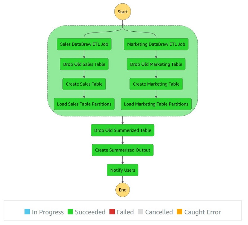
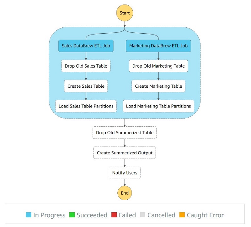
The following diagram is the visual representation of the state machine flow. With the Step Functions parallel task type, we created two parallel job runs for the sales and marketing data. When both flows are complete, they join to create an aggregated table in Athena and send an SNS notification to the end-users.

The following diagram is the visual representation of the state machine flow.

Creating an EventBridge scheduling rule

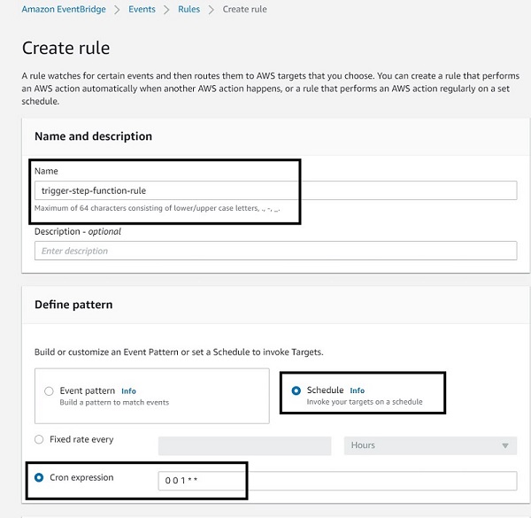
Now let’s integrate EventBridge to schedule the invocation of our Step Functions state machine on the first day of every month.

  1. On the EventBridge console, under Events, choose Rules.
  2. Choose Create a rule.
  3. For Name, enter a name (for example, trigger-step-funcion-rule).
  4. Under Define pattern, select Schedule.
  5. Select Cron expression.
  6. Enter 001** to specify that the job runs on the first day of every month at midnight.

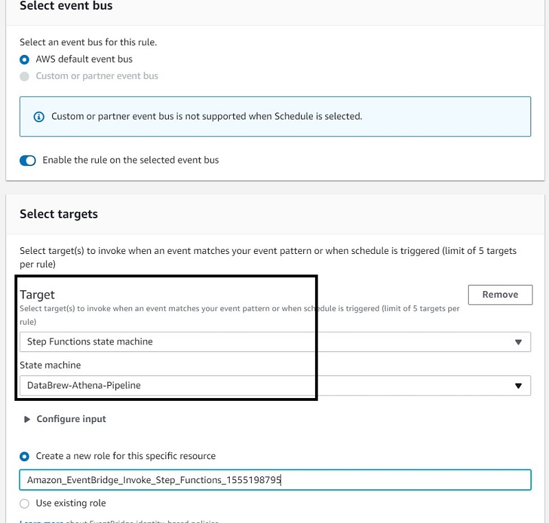
  1. In the Select targets section, for Target, choose Step Functions state machine
  2. For State machine, choose your state machine.

For State machine, choose your state machine.

Now when the step function is being invoked, its run flow looks like the following screenshot, where blue represents the DataBrew jobs currently running.

When the job is complete, all the steps should be green.

When the job is complete, all the steps should be green.

You also receive the notification “Monthly sales marketing data refreshed successfully!”

Running an Athena query

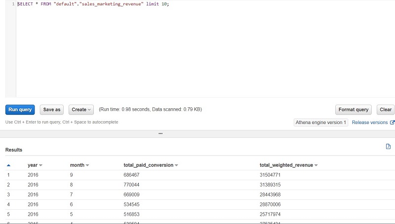
Let’s validate the aggregated table output in Athena by running a simple SELECT query. The following screenshot shows the output.

Let’s validate the aggregated table output in Athena by running a simple SELECT query.

Creating reports in QuickSight

Now let’s do our final step of the architecture, which is creating BI reports through QuickSight by connecting to the Athena aggregated table.

  1. On the QuickSight console, choose Athena as your data source.

On the QuickSight console, choose Athena as your data source.

  1. Select the database and table name you have in Athena.

Select the database and table name you have in Athena.

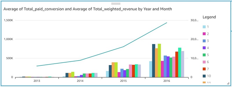
Now you can create a quick report to visualize your output, as shown in the following screenshot.

Now you can create a quick report to visualize your output, as shown in the following screenshot.


If QuickSight is using SPICE storage, you need to refresh the dataset in QuickSight after you receive notification about the completion of data refresh. If the QuickSight report is running an Athena query for every request, you might see a “table not found” error when data refresh is in progress. We recommend leveraging SPICE storage to get better performance.

Conclusion

This post explains how to integrate a DataBrew job and Athena queries with Step Functions to implement a simple ETL pipeline that refreshes aggregated sales and marketing data for BI reporting.

I hope this gives you a great starting point for using this solution with your datasets and applying business rules to build a complete serverless data analytics pipeline.


About the Author

Sakti Mishra

Sakti Mishra is a Senior Data Lab Solution Architect at AWS, where he helps customers architect data analytics solutions, which gives them an accelerated path towards modernization initiatives. Outside of work, Sakti enjoys learning new technologies, watching movies, and visiting places.