Greg Kroah-Hartman has released the 6.1.171, 5.15.205, and 5.10.255 stable kernels, quickly
followed by 6.1.172 and 5.15.206 kernels. This is another round
of stable kernels to provide fixes for one of the CVEs (CVE-2026-43284)
assigned following the Dirty
Frag and Copy Fail 2
security disclosures. There is not, yet, a stable kernel with a fix
for CVE-2026-43500,
though a
patch to fix the second half is in the works.
Every computer vision model is a reflection of the data it was trained on. The precision of the labels, the consistency across annotators, the coverage of edge cases. Get the data right and the model performs. Get it wrong and no amount of architecture or compute will compensate.
AI-assisted annotation tools have made it possible to label at a speed and scale that was unthinkable a few years ago. Teams that used to spend weeks on manual labeling now generate annotations automatically and refine them. That acceleration opens up real opportunity, but it also raises the bar for the infrastructure underneath the annotation pipeline. The architecture needs to keep pace with the volume of data now moving through it.
We have spent the last decade building AI workflows and one pattern shows up consistently: the teams that treat annotation as infrastructure from day one outperform the ones that bolt it on later. The difference is not just tooling. It is the architectural decisions underneath, particularly around storage, that determine whether an annotation operation scales or stalls.
Annotation within the ML pipeline
A production ML pipeline spans data ingestion, preprocessing, training, serving, and monitoring. Annotation sits within the data layer, but it is the stage where several consequential storage decisions converge: how raw data is stored, who can access it, how long it is retained, and how it flows between labeling, training, and evaluation. Getting storage right at this layer strengthens every stage downstream.
Data gravity. A single autonomous driving project can produce terabytes of camera and LiDAR data before a single label is applied. This data needs to live somewhere durable and accessible before, during, and after annotation. It rarely moves once it lands.
Collaboration. Labeling teams may be internal, external, or a mix. Quality reviewers need the same data access as annotators. The data layer has to support concurrent access across roles and geographies without creating bottlenecks or redundant copies.
Lifecycle persistence. Labeled datasets are reused across training runs, refined as models improve, and versioned as labeling standards evolve. Storage needs to retain raw data alongside annotations for months or years.
Regulatory constraints. In healthcare, automotive, and defense, access controls around training data are subject to compliance requirements. Encryption, scoped credentials, and auditability are non-negotiable.
The teams that design for these requirements upfront build data operations that scale cleanly across the entire pipeline.
CVAT as the annotation layer
CVAT (Computer Vision Annotation Tool) started as an internal tool at Intel in 2017, was open sourced in 2018, and spun out as CVAT.ai Corporation in 2022. Millions of users use it today, and for good reason.
Annotation breadth. CVAT covers the full range of label types: bounding boxes, polygons, polylines, keypoints, skeletons, cuboids, brush-based masks, and tags. It handles images, video, and 3D point clouds natively, so teams working across object detection, segmentation, and pose estimation stay on one platform instead of stitching separate tools together.
AI-assisted labeling. Beyond SAM 3 and YOLO, CVAT supports custom models through its AI Agents framework, which lets teams plug their own inference endpoints directly into the labeling workflow. For video, SAM 2-powered tracking propagates annotations across frames. The shift from manual annotation to review-and-correct workflows is where the real throughput gains happen.
Deployment flexibility. CVAT ships in three editions: Community (free, self-hosted), Online (managed SaaS), and Enterprise (on-premises with SSO, RBAC, and audit logging). You can start hosted and move to self-hosted as data governance needs evolve.
Pipeline integration. CVAT exposes a REST API with a Python SDK and CLI, so annotation tasks can be created, populated, and exported programmatically. For teams building CI/CD-style retraining loops, this is what makes CVAT a pipeline component rather than a standalone manual step.
Backblaze B2: The storage layer that compounds
Annotation tools get the attention, but the storage layer is where the architecture compounds over time. CVAT supports native cloud storage integration through S3-compatible buckets, and Backblaze B2 fits directly into that connector. Configure your B2 endpoint, bucket name, and application key credentials, and CVAT treats it as native cloud storage.
This architecture decouples compute from storage. CVAT handles annotation logic while B2 owns durability and access, and you can scale, migrate, or replace either independently. Because B2 is S3-compatible, other stages of the ML pipeline, from training scripts to data validation to orchestration, access the same data directly from the same bucket CVAT writes to. No intermediate exports. No dataset copies drifting out of sync.
Retention is where the storage decision pays off most. Annotation datasets have long lifecycles, and footprints accumulate fast across concurrent projects. B2’s storage economics let teams hold large datasets across the full model development lifecycle without cost becoming the limiting factor. This is especially relevant for video-heavy projects and multi-sensor datasets where raw data runs into tens of terabytes.
Access control matters too. B2 application keys can be scoped to individual buckets or file prefixes with granular permissions and optional expiration, so access boundaries stay clean across annotators, labeling services, and downstream training pipelines. The CVAT integration guide for Backblaze B2 walks through the full setup, and the CVAT cloud storage documentation covers access permissions, manifest files, and endpoint routing.
Building the pipeline that scales into what’s next
The teams building the best computer vision models are not just choosing better algorithms. They are investing in the annotation infrastructure that feeds those algorithms: the right labeling platform, the right storage architecture, and the right cost structure to sustain it all as data grows.
This becomes even more critical as the field moves toward world models. NVIDIA’s Cosmos platform has already been downloaded over two million times. World Labs launched Marble for commercial 3D world generation. DeepMind’s Genie 3 produces interactive 3D environments in real time. Yann LeCun left Meta to start AMI Labs with the explicit goal of building AI systems that understand physics, not just predict text. These systems need training data that goes far beyond today’s labeled images: synchronized multi-sensor captures, physics-aware video, dense 3D point cloud annotations. The data volumes and annotation complexity will dwarf what most teams work with today, and the infrastructure underneath will need to handle it.
The annotation pipeline you build now is the one that will carry you into that future. Both layers are worth getting right early.
This week’s Metasploit updates focused on foundational improvements and expanded target reach. Key enhancements were made to the recently released Copy Fail exploit module, which now benefits from payload fixes in linux/x64/exec and linux/armle/exec. These changes expand its capability, enabling the use of the cmd/unix/python/meterpreter/reverse_tcp payload on x64 targets and introducing support for ARMLE Linux. Additionally, the exploit/multi/http/shiro_rememberme_v124_deserialize module has been improved to allow operators to adjust the deserialization chain, enabling exploitation of a broader set of targets. Finally, several critical utility modules, including the FTP anonymous scanner and other FTP modules, received general fixes and updates.
Description: This updates the FTP anonymous scanner module. Key changes include moving the module to align with other generic FTP modules, adding and updating CVE references and documentation notes, and cleaning up the output to be more verbose. Additionally, the module now reports service and vulnerability data to the database and stores proof-of-exploitation info in the loot upon a successful run.
Enhanced Modules (2)
Modules which have either been enhanced, or renamed:
#21410 from inkognitobo – This improves the exploit/multi/http/shiro_rememberme_v124_deserialize module by adding a JAVA_GADGET_CHAIN datastore option that allows the operator to adjust the chain used for deserialization. This enables the module to exploit additional targets.
#21404 from zeroSteiner – This extends the support of Copy Fail to ARMLE Linux targets.
Enhancements and features (4)
#21342 from adfoster-r7 – Defers the loading of some dependencies to improve console boot time.
#21372 from g0tmi1k – This updates the FTP anonymous scanner module. Key changes include moving the module to align with other generic FTP modules, adding and updating CVE references and documentation notes, and cleaning up the output to be more verbose. Additionally, the module now reports service and vulnerability data to the database and stores proof-of-exploitation info in the loot upon a successful run.
#21380 from g0tmi1k – Updates multiple FTP modules to now register FTP service information in the database when successfully connecting to an FTP service.
#21418 from kx7m2qd – This improves the platform-agnostic library used to obtain the OS architecture with support for shell sessions on Linux, BSD and Mac OSX.
Bugs fixed (5)
#21314 from g0tmi1k – Fixes a crash when running the scanner/http/trace module with the database enabled and a vulnerability was reported.
#21411 from zeroSteiner – This fixes a bug in the linux/x64/exec payload that was caused by the CMD datastore option being placed in the assembly source without being escaped.
#21413 from tart0ru5 – Fixes a logic error in the exploits/linux/http/projectsend_unauth_rce module that incorrectly checked if a new user has been created.
#21421 from adfoster-r7 – This adds extra validation to report_vuln and delete_vuln in Msf::DBManager::Vuln to make sure required fields are present and avoid a crash.
#21425 from g0tmi1k – Fixes a bug when parsing FTP server responses.
Documentation
You can find the latest Metasploit documentation on our docsite at docs.metasploit.com.
Get it
As always, you can update to the latest Metasploit Framework with msfupdate and you can get more details on the changes since the last blog post from GitHub:
Analysis by the Anti-Corruption Data Collective, a non-profit research and advocacy group, found that long-shot bets—defined as wagers of $2,500 or more at odds of 35 percent or less—on the platform had an average win rate of around 52 percent in markets on military and defense actions.
That compares with a win rate of 25 percent across all politics-focused markets and just 14 percent for all markets on the platform as a whole.
It is absolutely insane that this is legal. We already know how insider betting warps sports. Insider betting warping politics—and military actions—is orders of magnitude worse.
An unusual, some might say hostile, approach to disclosing an alleged
remote-code-execution (RCE) flaw in the Forgejo software-collaboration platform has
sparked a multifaceted conversation. A so-called
“carrot disclosure” in April has raised questions about the
researcher’s methods of unveiling a security problem, Forgejo’s
security policies, and the project’s overall security posture.
At Netflix, we operate using a polyrepo strategy with tens of thousands of Java repositories. This means that we need to have ways of sharing common build logic across these repositories. On the JVM Ecosystem team within Java Platform, we build tooling such as the Nebula suite of Gradle plugins to provide standard ways to build projects, keep dependencies up-to-date, and publish artifacts reliably across the Java ecosystem. Our mission also entails providing build-time feedback to the developer when they deviate from the paved road, or when their code base contains technical debt.
Case Study
After a Netflix incident relating to a library releasing a backwards-incompatible change, our team was asked to provide some tooling and practices to improve the Java library lifecycle management. This was not a simple case of a library making a reckless breaking change. The code removed had been deprecated for years. Library authors often struggle to know when it is safe to remove deprecated code, or refactor code that is not meant to be used by downstream applications. Fleet-wide migrations, such as upgrading major Spring Boot versions, also involve deprecated code removal. To help with this, we established a suite of API lifecycle annotations:
@Deprecated from the Java standard library
@Public A custom annotation to use on APIs meant to be used downstream
@Experimental A custom annotation for new APIs which may not yet be stable
All other APIs are assumed to be “internal”
Library authors can annotate their APIs with these annotations. However, how will they know which downstream projects are using their API incorrectly, based on these?
As we sought to improve the paved road for JVM-based libraries at Netflix, we needed a good way of identifying this kind of technical debt, not only for the benefit of the Java Platform-provided libraries, but any team delivering shared libraries to the organization. For this, we looked at ArchUnit.
ArchUnit is a popular OSS library (3.5k stars, 84 contributors) used to enforce “architectural” code rules as part of a JUnit suite. It is used internally by Gradle, Spring, and is provided as part of the Spring Modulith platform. The rules engine, which is built directly on top of ASM, can be used for a wide variety of use cases. It is powerful enough to be a general purpose static analysis tool with the following distinctive features:
1. Works cross-language (JVM), because it uses ASM/bytecode, not AST parsing.
2. Exposes a builder API pattern that makes it easy to write rules
3. Also has a lower level API ideal for writing more complex custom rules.
The limitation of ArchUnit is that it is designed to be used as part of a JUnit suite in a single repository. The Nebula ArchRules plugins give organizations the ability to share and apply rules across any number of repositories. Rules can be sourced from OSS libraries or private internal libraries. This makes the plugin generally useful for any JVM+Gradle engineering organization.
Why ArchUnit?
Before we go into how ArchRules works, it is good to understand why we would want to use ArchUnit in this way instead of other static analysis tools.
AST vs Bytecode
Some tools, such as PMD, process rules against an AST (abstract syntax tree). An AST is a structured representation of source code. This kind of tool will have rules that are syntax dependent. Rules that need to support multiple JVM languages, such as Kotlin or Scala, often need to be rewritten for each language. It also allows code which should be found to be hidden under syntactic sugar not anticipated by the rule author. ArchUnit uses ASM to analyze actual compiled bytecode, which means it doesn’t matter how that code was produced. What is analyzed is the actual code that will be run.
Rule Authorship
Tools like PMD and Spotbugs are not optimized for custom rule authorships. Most usage of these tools run built-in provided rules, or add in pre-made third party plugins. Take a look at what a custom rule for PMD might look like:
<![CDATA[
 //AllocationExpression/ClassOrInterfaceType[
   @Image='DateTime' and (
       (count(..//Name[@Image='DateTimeZone.UTC'])<=0)
       and
       (count(..//Name[@Image='DateTimeZone.forID'])<=0)
    ) or (
       (
           (count(..//Name[@Image='DateTimeZone.UTC'])>0)
             or
           (count(..//Name[@Image='DateTimeZone.forID'])>0)
       ) and (../Arguments/ArgumentList and count(../Arguments/ArgumentList/Expression) = 1)
   )
 ]
]]>
This rule ensures that DateTimes are not instantiated without an explicit zone. This is a raw string meant to be used within PMD’s xpath parser. There is no IDE guidance on crafting it. To test it, a whole separate PMD process needs to be wired up to interpret the rule and evaluate it against a source file. Let’s see how a similar rule would look with ArchUnit:
ArchRuleDefinition.priority(Priority.MEDIUM)
.noClasses()
.should()
.callConstructorWhere(
    // constructor does not have a zone arguement
    target(doesNot(have(rawParameterTypes(DateTimeZone.class))))
   // constructor is for DateTime
        .and(targetOwner(assignableTo(DateTime.class)))
)
This is type-safe Java code with a fluent API. It is also simple to unit test, as ArchUnit has a method to pass a rule object and class references to evaluate the rule against those classes.
Class Relations
Because ArchUnit processes the entire classpath with ASM, it retains a graph of the class data, allowing rules to easily traverse class relationships and call sites. This allows rules to have much more context about the code it is evaluating.
Rules Libraries
The first step was to build the ability to write ArchUnit rules which can be shared and published. In order to do this, we have the ArchRules Library Plugin. This plugin adds an additional source set to your Gradle project called archRules. In this source set, you can create a class which implements the ArchRulesService interface. This interface has a single abstract method which returns a Map<String, ArchRule>. The keys of this map are the names of your rules, and the ArchRule is the rule you would like to define using the standard ArchUnit API. Here is an example:
public class GuavaRules implements ArchRulesService {
  static final ArchRule OPTIONAL = ArchRuleDefinition.priority(Priority.MEDIUM)
        .noClasses()
        .should()
        .dependOnClassesThat()
        .haveFullyQualifiedName("com.google.common.base.Optional")
        .because("Java Optional is preferred over Guava Optional");

    @Override
    public Map<String, ArchRule> getRules() {
        Map<String, ArchRule> rules = new HashMap<>();
        rules.put("guava optional", OPTIONAL);
        return rules;
    }
}
This code and its dependencies will not be bundled with your main code. It is bundled into a separate Jar with the arch-rules classifier. When publishing, your library will publish this jar as a separate variant with the usage attribute set to arch-rules. This means that in order for downstream projects to use these rules, they must use Gradle Module Metadata for dependency resolution. There are 2 flavors of rules Libraries: Standalone rules libraries, bundled rule libraries.
Standalone Rule Libraries
A Standalone Rule library contains no main code: only archRules. These are useful for defining rules for code you don’t own, such as Core Java APIs or OSS libraries. They are also useful for generic rules that can apply to any code, such as “don’t use code marked as @Deprecated”. We maintain a collection of OSS Standalone rule libraries which anyone is free to use, and serve as examples of the types of rules you may want to write yourself. However, the real power of ArchRules is in “bundled rule libraries”.
Bundled Rule Libraries
A bundled rule library is a library with both main and archRules sources. The main source set will contain useful library code, whatever it may be. The archRules will contain rules specific to the usage of that library. For example, rules scoped to that library’s package, or referencing that library’s specific API. Whenever possible, we recommend writing rules in this bundled way. That is because the ArchRules Runner Plugin will be able to automatically detect these rules and run them in only the source sets that use this library as a dependency. An example of this can be seen in our Nebula Test library.
In any case, the library plugin will automatically generate a service loader registration entry for your ArchRulesService so that the runner can discover your rules.
Running Rules
The ArchRules Runner Plugin allows rules to be evaluated against your code. Standalone rule libraries can be evaluated against all source sets by adding them to the archRules configuration in your build. For example:
dependencies {
    archRules("your:rules:1.0.0")
}
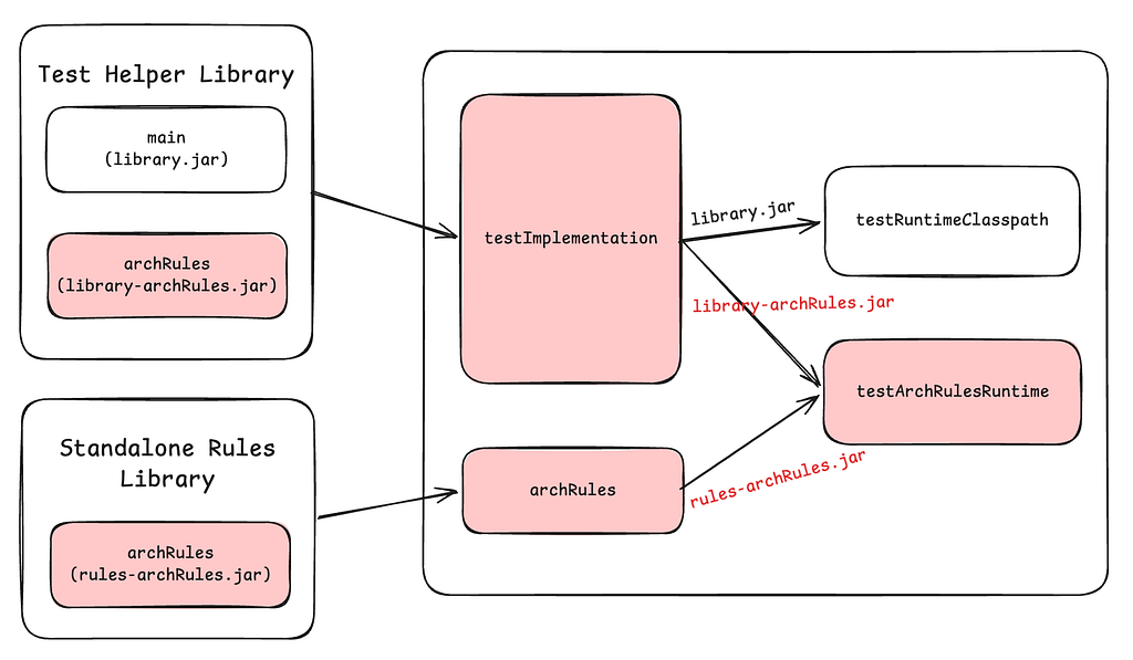
As mentioned before, bundled rules will be evaluated automatically. To do this, the runner plugin creates a separate configuration for each of your source sets. In each of these configurations, the archRules classpath is combined with the runtimeClasspath with the arch-rules variant selected. This configuration is the classpath used when the ServiceLoader discovers implementations of ArchRulesService. In the following example, we have a Project which uses a test helper library as a testImplementation dependency, and also adds a standalone rules library to the archRules configuration. The test runtime classpath will only contain the implementation jar for the helper library, but the arch rules runtime will contain the archrules jar for the bundled rules and standalone rules. This all happens automatically.
Gradle configurations used by ArchRules
Once the rules classpath is determined, the runner plugin will create a Gradle work action to evaluate rules against that specific source set. This action runs with classpath isolation using the *archRuleRuntime configuration. Within this action, a ServiceLoader is used to discover rule definitions. The action ends by writing a binary serialization of rule violations to a file for reporting.
In a project running rules, you also have the ability to customize rule configurations using the archRules extension. For example, you can override a rule’s priority level:
Other customizations include disabling running rules on certain source sets and configuring the failure threshold (i.e., high priority failures will cause the build to fail).
Reporting
The ArchRules runner plugin has two built-in reports: JSON and console. The json report will collect the output from all source sets within a project and create a single json file with all of the data. The console report also collects the output from all source sets within a project, but it prints to the console an easy to read report, for example:
Console Report output
Note that failure details feature a detailed plain English description, along with a pointer to the exact line of code in violation.
For custom reporting, you can either use the JSON file, or create your own task that reads the binary files. Take a look at the source code for the ArchRules runner plugin’s report tasks for an example of how to do this.
Case Study Solution
Going back to our original problem, using ArchRules, we were able to deliver a platform for library authors to track the usage of their APIs. They write ArchRules to detect usage of the annotations, scoped to their library’s package, such as:
ArchRuleDefinition.priority(Priority.MEDIUM)
    .noClasses().that(resideOutsideOfPackage(packageName + ".."))
    .should()
    .dependOnClassesThat(resideInAPackage(packageName + "..").and(are(deprecated())))
    .orShould().accessTargetWhere(targetOwner(resideInAPackage(packageName + ".."))
        .and(target(is(deprecated())).or(targetOwner(is(deprecated())))))
    .allowEmptyShould(true)
    .because("Deprecated APIs are subject to removal");
Our internal Nebula standard Gradle wrapper and plugin suite automatically enable the ArchRules runner on every project, and provides a custom reporter which sends the report data to our Internal Developer Portal on every main-branch CI build. This way, library authors can easily see a report of all downstream consumers using their experimental, deprecated, or non-public APIs, giving them confidence to make “breaking” changes, knowing that it will not actually break downstream consumers. If their changes are currently blocked by downstream usage, they can easily see exactly which projects are reporting those usages.
OSS Rule Libraries
While the most powerful way to use ArchRules is for you to write your own rules, we have built some OSS rule libraries that anyone is free to use, or reference as examples.
Nullability
These rules enforce proper nullability annotation in Java, for example, that every public class is marked with JSpecify’s @NullMarked. It is smart enough to exclude Kotlin code, as Kotlin has built-in nullability.
Gradle Plugin Best Practices
Writing Gradle plugins can be hard, especially since there are many APIs and patterns that should not be used anymore. These rules help enforce current best practices when writing Gradle plugins.
Joda / Guava Rules
These rule libraries discourage the use of Joda Time and Guava classes (respectively) as these have been superseded by java.time and standard library enhancements.
Security Rules
These rules help mitigate CVEs by detecting usage of known vulnerable APIs. Ideally, we keep dependencies up to date to mitigate CVEs. But sometimes that is not immediately feasible, and in those cases, a compile time check to ensure the specific vulnerable API is not used is often good enough.
Conclusion
We are now running 358 (and counting) rules across over 5,000 repositories detecting over nearly 1 million issues. About 1,000 of these issues are for “High” priority rules. Being able to run these rules on this scale allows us to quickly gain insight into our large fleet of microservices, and identify the areas carrying the most critical technical debt. This makes it easier to focus and prioritize our efforts.
Going forward, we will be exploring how to tie auto-remediation solutions into the ArchRules findings. ArchUnit currently provides very specific and detailed information about failures in reports, which makes a very strong input signal to an auto remediation tool. We will explore deterministic solutions such as OpenRewrite and non-deterministic solutions such as LLMs. Pairing the easy rule authorship and deterministic results of ArchUnit with an auto-remediation tool that can correctly interpret the results to solve the issue at hand will be a very powerful combination.
We also will investigate how to get ArchRule failure information surfaced in the IDE as inspections.
If you have questions or feedback about Nebula ArchRules, reach out to us by posting in the #nebula channel on the Gradle Community Slack.
As modern applications evolve into complex ecosystems of serverless functions, microservices, and event-driven architectures, incident response becomes increasingly challenging. DevOps and SRE teams spend hours manually correlating data across observability tools and troubleshooting issues, racing against SLA deadlines. This reactive firefighting drains productivity, degrades reliability, and delays innovation.
AWS DevOps Agent provides an opportunity to shift how teams achieve operational excellence. As an autonomous, always-on frontier agent, it investigates incidents the moment they occur, identifies root causes by correlating telemetry across your ecosystem, and recommends specific mitigation plans, all without constant human intervention. On-call engineers wake up to a root cause, instead of active incidents. AWS DevOps Agent supports multi-cloud and hybrid environments, not just AWS-native architectures.
This blog post demonstrates how to build an end-to-end agentic SRE solution using AWS DevOps Agent. You learn how to configure DevOps Agent Spaces that define an investigation scope, integrating seamlessly with Amazon CloudWatch, Splunk, GitHub, and Slack. It further demonstrates automated incident trigger using webhooks, and AWS DevOps Agent integration with custom tools by creating a custom MCP agent. The agent investigates issues by analyzing patterns across multiple data sources, providing root cause, and then generates detailed mitigation plans that can be implemented via a coding agent. By the end, you will have a deployed frontier agent that acts as a true extension of your team. One that works persistently, scales massively, and delivers complete operational outcomes while freeing your engineers to focus on innovation rather than firefighting.
Architecture
Implementation
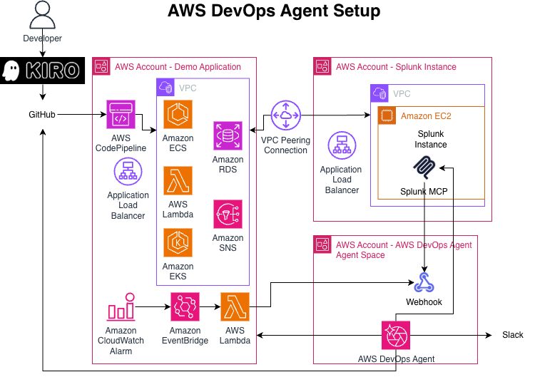
This implementation spans three specialized AWS accounts with distinct responsibilities.
The Demo Application account hosts the production infrastructure being monitored. The CI/CD pipeline integrates GitHub via AWS CodePipeline for automated deployments, while an Application Load Balancer distributes traffic and monitors health. The observability layer leverages Amazon CloudWatch alarms to detect anomalies, Amazon EventBridge to route events, and AWS Lambda as a webhook handler that forwards incident notifications to AWS DevOps Agent.
The account named Splunk provides centralized log aggregation and analysis. An Amazon EC2 instance hosts the Splunk Log Collector, while Splunk MCP manages the centralized control plane. A VPC peering connection establishes secure, private network connectivity between the Demo Application and Splunk account VPCs, enabling seamless log forwarding, without internet exposure.
AWS DevOps Agent account contains the autonomous investigation engine. AWS DevOps Agent receives incident webhooks from the Demo Application account, orchestrates autonomous investigations across integrated data sources, correlates telemetry from CloudWatch, Splunk, and GitHub, generates mitigation plans, and coordinates the incident response. The webhook integration provides communication, receiving incident triggers from Lambda, and sending investigation updates to Slack for real-time team collaboration.
Data flow: When an incident triggers the CloudWatch alarm, EventBridge invokes a Lambda function that, in turn, invokes the DevOps Agent webhook with a payload. The agent triggers an investigation based on its native troubleshooting capabilities. For a comprehensive view of the incident, it queries Splunk logs via MCP, retrieves deployment history from GitHub, and correlates CloudWatch metrics with deployment events to build application topology understanding. It analyzes temporal relationships between deployments and operational incidents, identifies root causes, and generates detailed mitigation plans with specific remediation steps, success criteria, and rollback procedures via Splunk MCP. The DevOps Agent’s runbooks/skills guide its investigation from start to finish, keeping it on track and aligned with established SRE procedures. Investigation results and recommendations are posted to Slack, enabling on-call engineers to wake up to identified root cause, instead of active incidents.
Creating your agentic DevOps engineer
DevOps Agent Spaces
A DevOps Agent Space defines the tools and infrastructure that AWS DevOps Agent has access to. Each Agent Space contains your AWS account configurations, third-party tool integrations, and access permissions. See Best Practices for Deploying AWS DevOps Agent in Production for detailed information describing the DevOps Agent spaces.
Creating an Agent Space can be done through the console, or via AWS Command Line Interface (AWS CLI). You should name your Agent Space with a descriptive name to identify its purpose. For example, if your application is “WidgetMaker”, then you can name your Agent Space “WidgetMaker Agent” to help you quickly identify the context of that agent.
Follow the steps in Creating an Agent Space for details and considerations when creating an Agent Space.
Agent Space webhooks
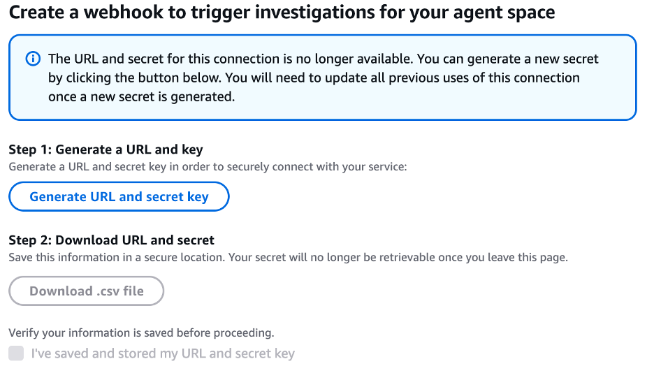
Before connecting any services to your DevOps Agent Space, make sure to create the webhook for your Agent Space. The schema for you to send messages to your Agent Space is shown below:
Make sure you download and save this unique url and secret key. Once you move on from this screen, you will no longer be able to see the secret. Now that we’ve created the webhook endpoint, we will set up the alarm or choose an existing alarm. Then we will use an Amazon Simple Notification Service (Amazon SNS) topic as the Alarm Action and subscribe a Lambda function to this topic. The Lambda function then calls the webhook. Store the webhook URL in Lambda environment variables for security.
The CloudWatch flow is: CloudWatch Alarm → Amazon EventBridge → Lambda → DevOps Agent Webhook.
Test by forcing the alarm into the ALARM state and verifying the DevOps Agent receives the event. See some samples on sending these alarms via WebHook at the aws-samples github.
Splunk Integration
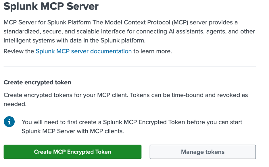
For Splunk integration, you will need to perform a few tasks on your Splunk server. First, you will need to enable the Splunk MCP Server to expose the MCP URL for AWS DevOps Agent.
For Splunk MCP Server, you will first configure a token to allow AWS DevOps Agent to securely log into the Splunk MCP server.
Note: You will need to have a role called ‘mcp_user’ (it doesn’t need any capabilities) and add it to the user account in Splunk that you are going to create the token in the next step.
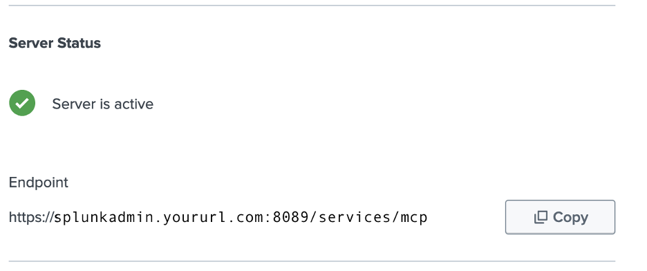
The audience should default to ‘mcp’ on this screen, but if not, audience will need to be ‘mcp’. Remember, you must copy the token from the screen when you create the token, or you will not be able to access it after you close the screen, requiring you to create a new token. Then, you can validate that the endpoint is active and copy the endpoint url. Note, the url presented reflects the url that you are using for the Splunk management console. If you have created a listener on port 8089 with a different url, for example, https://splunkmcp.yoururl.com:8089, then you will need to replace the url shown (https://splunkadmin.yoururl.com) with the proper url.
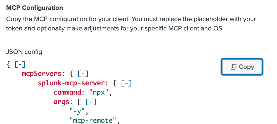
Finally, copy the MCP Configuration for use in AWS DevOps Agent. Note, just as above, validate that the url is the same as the listener you have created. Also, reminder to replace <Your Token> with the bearer token you’ve created (and copied) above.
To configure Splunk to send alerts to AWS DevOps Agent to begin investigations, you will need to use Better Webhooks because the default Splunk webhook does not support headers nor authentication.
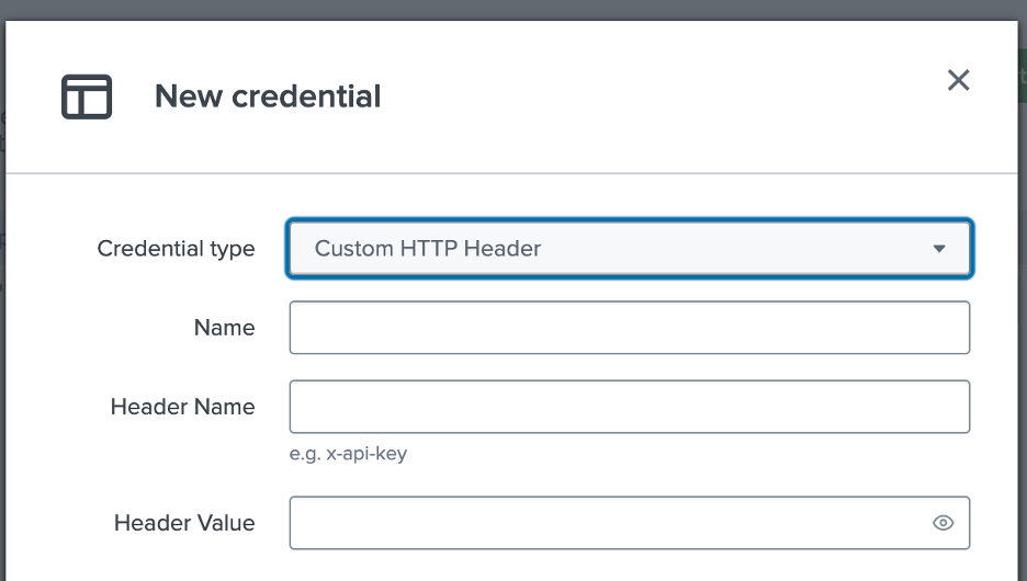
Once you have Better Webhooks, you can create a credential and choose Custom HTTP Header. Name can be whatever you desire, but we used “DevOpsAgentBearer” to be descriptive.
Header Name: Authorization
Header Value: “Bearer thetokenyousavedwhenyoucreateddevopsagentwebhook” (Include “Bearer” and a space before your token from your DevOps Agent webhook)
You can skip the advanced section and save your credential.
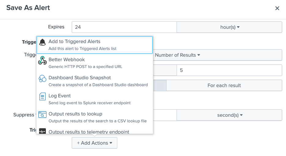
Now, you can configure the alert for your error state by finding it in search and saving search as an alert. Under Trigger Actions, select Add Actions and choose Better Webhook from the menu.
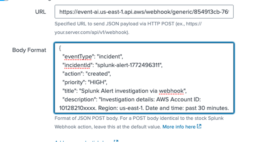
Then, format the message body as shown in AWS DevOps Agent.
In Splunk, the URL is the DevOps Agent webhook url which you had saved in a .csv with your token while creating the webhook. Paste the format above into the Body Format section as shown below, select the credential you saved in Better Webhooks earlier, and save your alert.
Notice that the Body Format box should reflect the format from AWS DevOps Agent above. Now, AWS DevOps Agent will initiate an investigation when Splunk errors exceed the threshold for the alert you’ve created. You may want to experiment with throttling and thresholds to keep AWS DevOps Agent from starting too many investigations.
Connecting to Slack
You can connect AWS DevOps Agent to your Slack environment and configure a channel for your Agent Space to communicate with. You can have multiple Agent Spaces communicate in one Slack channel, or you can have existing Slack channels for your SRE team invite the Agent Space to it.
To get started, you need to have access to a Slack workspace with the ability to install and authorize third-party applications. You then need to go to the AWS DevOps Agent console, navigate to “Settings” and select “Communications”. When you choose Register, you will be redirected to Slack to authorize the AWS DevOps Agent application for your workspace. It is important to install at the workspace level, not in your enterprise grid.
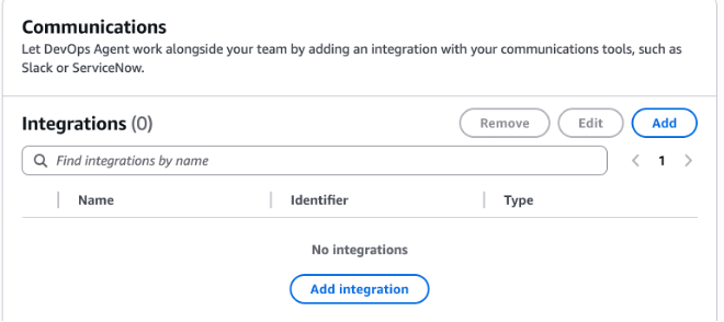
After you choose Allow, you will be directed back to your DevOps Agent console to associate your Agent Space with your Slack channel. Go to your Agent Space, scroll down to Communications, and choose Add integration.
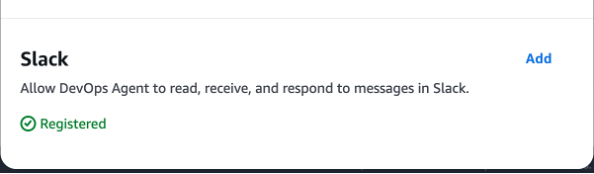
Towards the bottom of the popup, you should see Slack and it should show “Registered” in green.
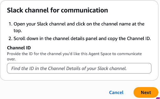
Choose Add and follow the instructions in the window to obtain and insert your channel ID into the DevOps Agent Space.
Once completed, you just need to add the AWS DevOps Agent to your channel by typing the following into your Slack channel: /invite @AWS DevOps Agent
Now, you can start an investigation, and the AWS DevOps Agent will provide details in your channel.
Connecting GitHub to AWS DevOps Agent
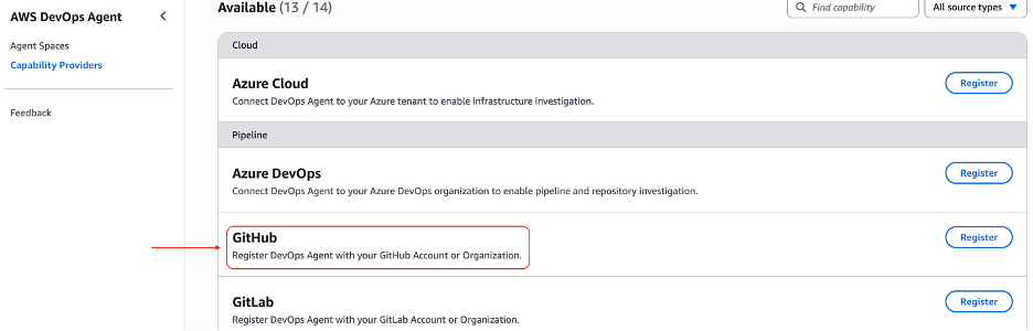
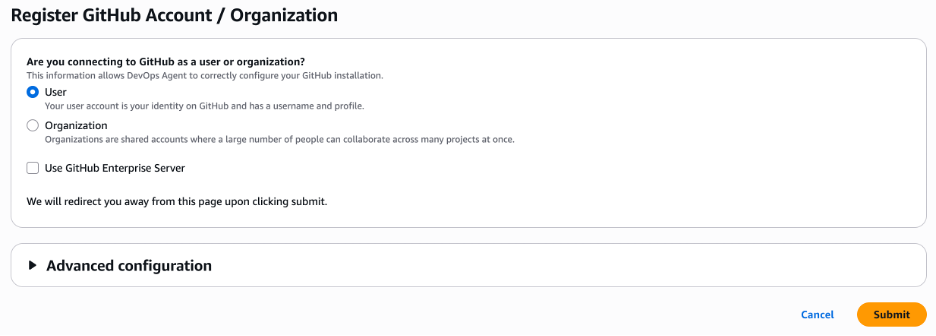
GitHub integration is a two-step process. First, register GitHub at the AWS account level: navigate to your Agent Space’s Capabilities tab, select Add under Pipeline, choose GitHub, and complete the OAuth flow to install the AWS DevOps Agent GitHub app. You can select which repositories the app can access — all or a specific subset. Once registered, connect repositories to individual Agent Spaces by selecting the relevant repos under the Pipeline section. The GitHub app requests read-only access and receive deployment events, enabling the agent to correlate code changes with operational incidents.
DevOps Agent Skills
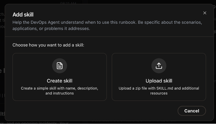
You can use DevOps Agent Skills to define a set of rules for all investigations to follow, guiding the Agent to use certain documentation, or telemetry sources for certain types of data. Skills are self-contained directories containing Markdown instructions that provide specialized capabilities to AWS DevOps Agent. AWS DevOps Agent supports a subset of the Agent Skills specification — an open standard for packaging agent instructions and resources—supporting only non-executable documents: Markdown instructions, PDFs, images, and data files. For example, if your environment uses Dynatrace for alarms and metrics, Splunk for logs, and CloudWatch for serverless logs, create a skill to accelerate issue resolution. You create these Skills in your Operator console by selecting the Skills section on the lower left side of the screen. You can then either review your existing skills or use the Add skill button to choose between Create skill and Upload skill options.
The documentation on DevOps Agent Skills should help you with the schema and best practices in creating these skills.
Investigate root cause
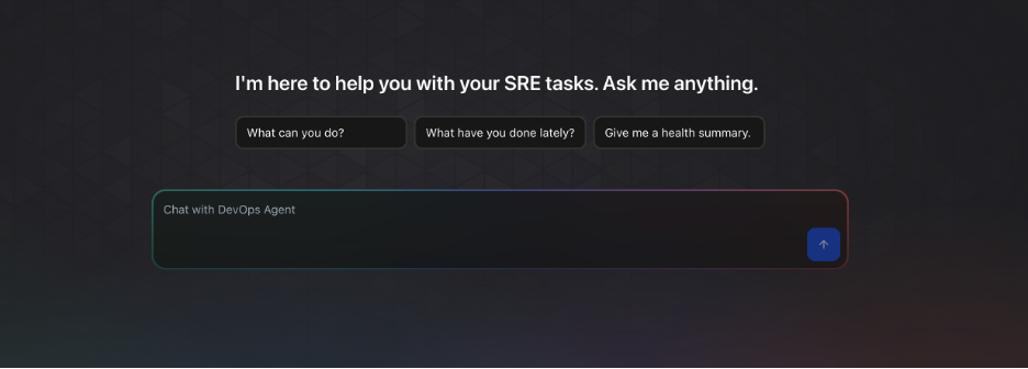
Now that you have everything connected to your DevOps Agent Space, you can interact with the AWS DevOps Agent you’ve created. You can investigate anomalies in your environment, or have alarms trigger your Agent to begin an investigation on its own and provide updates in your Slack channel and the Operator console. You can also ask the agent to provide health summaries, suggest preventive maintenance, and other SRE tasks you would do throughout the lifecycle. You can do this in the operator console and simply type your question into the Chat with DevOps Agent box. For example, “What is causing high CPU usage on my EC2 instances starting an hour ago?” and the AWS DevOps Agent will begin investigating your request.
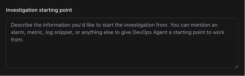
While optional, the steps below can help speed up a particular investigation and help track multiple investigations. Adding an Investigation starting point can help speed up the investigation by telling the agent to check a particular alarm, or an Autoscaling Group (ASG), or even a specific set of instances where you are seeing increased CPU usage. This guides the investigation to start with data sources pertaining to these resources, instead of looking at all your telemetry to find anomalies to start investigating.
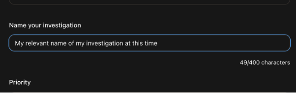
You should also make a habit of assigning a meaningful name to your investigations, so that you can look at the historical data with some context.
Generating mitigation plan
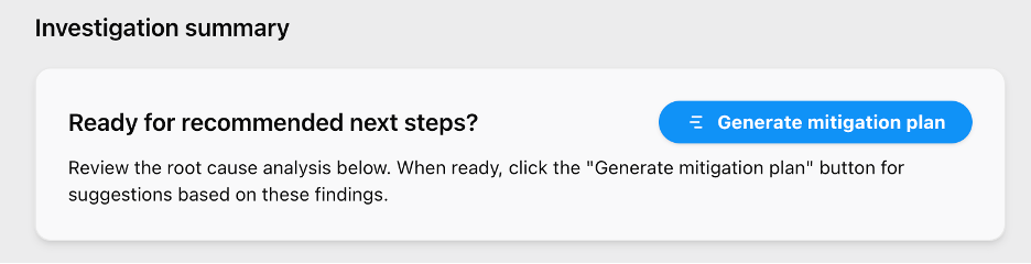
A mitigation plan is a set of actionable steps that AWS DevOps Agent produces to resolve an identified incident. After the agent publishes a root cause under the Root Cause tab, select “Generate mitigation plan” to create a structured remediation plan. Alternatively, automate this step using the AWS CLI — use aws devopsagent create-backlog-task to trigger investigations and update-backlog-task to approve mitigation plans programmatically. By automating this step, you can integrate mitigation plan generation directly within their incident workflow, without having to leave their incident management application. The CLI returns the mitigation steps back into the integrated app or system. Each plan follows four phases: Prepare, Pre-Validate, Apply, and Post-Validate. Within each phase, the agent provides suggested actions with commands to update infrastructure-as-code templates or make configuration changes. It also generates agent-ready specs compatible with coding agents like Kiro for implementation.
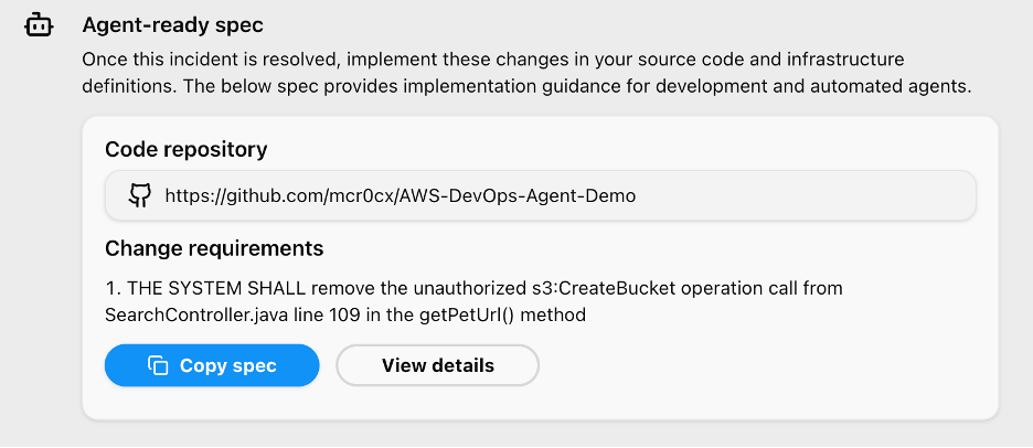
Agent-ready Spec and fix implementation
An agent-ready spec is a structured set of instructions that AWS DevOps Agent generates within a mitigation plan, designed to be consumed directly by a coding agent. When the mitigation plan includes code-level fixes — such as updating infrastructure-as-code templates or application logic — AWS DevOps Agent produces these specs alongside the suggested actions. To apply a fix, copy the agent-ready spec and hand it off to a compatible coding agent like Kiro. The coding agent interprets the spec and implements the required changes in your codebase. This creates a seamless handoff from incident diagnosis to code remediation, closing the loop between identifying a root cause and deploying the fix without manually translating mitigation steps into code changes.
Conclusion
In this post, we demonstrated building an end-to-end agentic SRE solution using AWS DevOps Agent — from configuring Agent Spaces and integrating CloudWatch, Splunk, GitHub, and Slack, to triggering automated investigations via webhooks, generating mitigation plans, and handing off agent-ready specs to coding agents like Kiro for implementation. Together, these capabilities shift incident response from reactive firefighting to autonomous resolution, reducing MTTR from hours to minutes while freeing your engineers to focus on innovation.
You might have data in Amazon Simple Storage Service (Amazon S3) buckets in different AWS Regions that you want available in a single Amazon OpenSearch Service domain or collection. Consolidating data across Regions provides unified analytics and searches, reduce operation complexity, and streamline your search infrastructure. We’re happy to announce that Amazon OpenSearch Ingestion pipelines can now read from S3 buckets in different Regions to ingest and consolidate data into a single OpenSearch Service domain or collection.
To consolidate this data across AWS Regions, you previously had to provide your own solution. Now Amazon OpenSearch Ingestion can help you accomplish this. In this post, I’ll show you how to use the new cross-Region support to ingest data from S3 buckets across multiple AWS Regions into a single OpenSearch Service domain or collection.
Amazon OpenSearch Ingestion (OSI) is a feature-rich data ingestion pipeline that you can use for many different purposes: observability, analytics, and zero-ETL search. Many customers use OpenSearch Ingestion to ingest data from Amazon S3 into OpenSearch Service domains and Amazon OpenSearch Serverless collections. Until now, you could only ingest from a single AWS Region at a time. Now that you can use OpenSearch Ingestion for cross-Region S3 ingestion, I’ll show you how you can use it in two scenarios: batch processing using S3 scan, and streaming ingestion using Amazon Simple Queue Service (Amazon SQS) queues for AWS vended logs like Amazon Virtual Private Cloud (Amazon VPC) Flow Logs and AWS CloudTrail.
You need S3 buckets in at least two different Regions. You can use existing ones or create S3 buckets. You can use one in the same AWS Region as your OpenSearch Service domain or collection, or use two completely different Regions.
Upload objects with data into your S3 buckets. The data can be JSON, ND-JSON, Parquet, CSV, or plaintext formats.
For cross-Region ingestion, you must now also include the s3:GetBucketLocation permission. This gives the pipeline the ability to determine which AWS Region the bucket is located in.
After you complete these steps, you can either set up your Amazon OpenSearch Ingestion pipelines for batch or streaming scenarios. In the following sections, I’ll give you recommendations on when to choose which approach, and I outline the steps for creating your pipeline.
Batch scenarios
You can use the OpenSearch Ingestion S3 scan capability to read batch data from S3. You might find this approach useful when your data is written to S3 on a schedule. To perform a cross-Region S3 scan, you only specify the buckets that you’re reading from when you create the OpenSearch Ingestion pipeline.
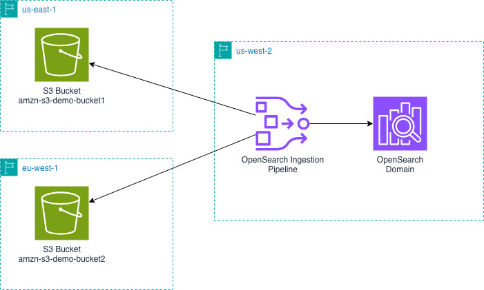
The following diagram shows the design for an OpenSearch Ingestion pipeline in us-west-2 reading from S3 buckets in us-east-1 and eu-west-1 and writing that data into an OpenSearch Service domain in us-west-2.
The previous pipeline configuration supports the JSON codec. You might want to configure a different codec if your data isn’t a large JSON object.
You can now query your OpenSearch Service domain or collection to see the data that you ingested.
Streaming scenarios: AWS vended logs
Like many of our customers, you might want to ingest S3 data from different AWS Regions into OpenSearch Service. A common reason is to consolidate AWS vended logs. For example, VPC Flow Logs, CloudTrail data, and load balancer logs. For these scenarios, you can configure OpenSearch Ingestion pipelines to read from an Amazon SQS queue to stream data into your OpenSearch Service domain or collection.
These AWS vended logs write to Amazon S3 in the same AWS Region as the service running it. For example, VPC Flow Logs will be in the same AWS Region as your Amazon VPC. You can use OpenSearch Ingestion to consolidate these logs into one AWS Region. In the VPC Flow Logs example, you can consolidate your VPC Flow Logs from multiple AWS Regions into a single OpenSearch Service domain or collection to analyze network patterns from your different Amazon VPCs.
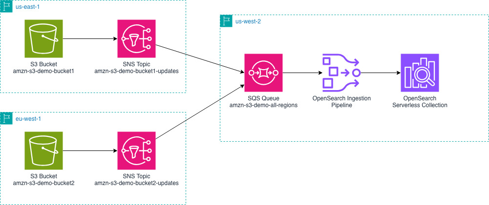
The following diagram outlines the overall setup. It shows an example of sending AWS vended logs from us-east-1 and eu-west-1 to an OpenSearch Service domain in us-west-2. You can change the AWS Regions depending on your specific needs.
You must configure your vended logs to write log events to Amazon S3 buckets in their respective AWS Regions. Using VPC Flow Logs as our example, you can configure VPC Flow Logs for your VPCs.
Amazon S3 doesn’t send notifications to cross-Region Amazon SQS queues, so you will use intermediate Amazon Simple Notification Service (Amazon SNS) topics to consolidate the notifications from multiple Regions into one queue. For each S3 bucket, create an SNS topic.
SNS can send cross-Region notifications to SQS. Create a subscription from each SNS topic that you created in step 3 to the single SQS queue you created in step 2.
Configure your pipeline role to read from SQS and read from the relevant S3 buckets.
The previous pipeline configuration supports the JSON codec. You might want to configure a different codec if your data is not a large JSON object.
Next, upload objects with data into your S3 buckets. By uploading data, S3 will send notifications to SNS and then the SQS queue.
You can now query your OpenSearch Service domain or collection to see the data that you ingested.
Here is what makes this possible and what is different. The SQS queue receives the event notifications for the buckets. Before the cross-Region feature of OpenSearch Ingestion, the pipeline could see these events, but couldn’t access the S3 bucket even if the permissions were granted. Now, the pipeline will determine the AWS Region that the bucket is in, access an AWS Security Token Service (AWS STS) token for the AWS Region of the bucket. Using the STS token from the same Region as the S3 bucket allows the pipeline to read and access the data.
Using the AWS Console
When you create the pipeline using the OpenSearch Ingestion console, you will have options to select a blueprint for your use-case. These blueprints help you create pipelines for various vended log types only by selecting your SQS queue and OpenSearch domain. The blueprint handles the data type mappings for you by including appropriate processors. You can use these blueprints as a starting point and modify your processors for your specific requirements.
Clean up resources
When you’re done testing this out, use the following resources to delete the resources that you created.
If you configured AWS vended logs you can delete those logging configurations. This example used VPC Flow Logs. For instructions on how to do so, see Delete the Flow Logs.
For both pipelines, these steps help you delete the common resources.
In this post, I showed you how you can use Amazon OpenSearch Ingestion to ingest data from Amazon S3 buckets in different AWS Regions. I showed that this works for both batch scan and streaming scenarios. The feature offers you a straightforward way to consolidate your data from other Regions into one OpenSearch Service domain or collection.
To get started with the cross-Region S3 source, refer to the OpenSearch Ingestion documentation or try creating a pipeline from one of our blueprints using the OpenSearch Ingestion console. You can read about the codecs that OpenSearch Ingestion offers for parsing your S3 objects. You can also learn how about the various processors that OpenSearch Ingestion offers, so you can transform and enrich your data to meet your needs.
You can also use OpenSearch Ingestion for cross-Region and cross-account. To do this, you must grant cross-account permissions on your S3 bucket. You must also make some changes to your pipeline configuration. Combining what I showed you in this post with the existing cross-account features greatly expands your ingestion options.
It seems that we are in for an extended period of the disclosure of
vulnerabilities before fixes become available. One possible way of coping
with this flood might be the killswitch
proposal from Sasha Levin. In short, killswitch can immediately disable
access to specific functionality in a running kernel, essentially blasting
a vulnerable path (and its associated functionality) out of existence until
a fix can be installed. “For most users, the cost of ‘this socket
family stops working for the day’ is much smaller than the cost of running
a known vulnerable kernel until the fix land.“
This is a guest post by Supreet Padhi, Technology Architect, Strategic Technologies, and Rochelle Grubbs, Senior Director, Solution Architect at Precisely in partnership with AWS.
Business leaders face a critical challenge to enable real-time analytics. Their most valuable data sits in mainframe systems that reliably process billions of transactions daily, but extracting value for modern analytics and AI remains complex and costly. Traditional mainframe-to-cloud integration approaches require multi-step replication with intermediary systems, creating operational overhead, latency, and data integrity risks. This complexity delays insights, increases infrastructure costs, limits agility, and blocks organizations from using AI and machine learning on their mainframe data.
Organizations that can connect their mainframe environments with modern cloud platforms can gain advantages through improved agility, reduced operational costs, and enhanced analytics capabilities.For example, moving appropriate analytics and reporting workloads to the cloud can significantly reduce mainframe operational costs while maintaining performance and reliability. Real-time data access makes insights available within seconds rather than waiting for batch processing cycles, enabling faster responses to market changes and customer needs. Eliminating bulk data extracts and intermediary systems also reduces infrastructure and maintenance expenses. This frees IT resources to focus on higher-value initiatives.
However, implementing mainframe-to-cloud integrations presents unique technical challenges that require specialized solutions. These include converting mainframe character encoding (EBCDIC) to standard ASCII format and handling mainframe-specific data types such as packed decimal (COMP) fields. You also need to manage the complexity of VSAM (Virtual Storage Access Method) files that can store multiple record types in a single file, and maintain real-time synchronization without impacting mainframe performance.
Change Data Capture (CDC) technology addresses these challenges through incremental data movement that eliminates disruptive bulk extracts by streaming only changed data to cloud targets, minimizing system impact and ensuring data currency. Real-time synchronization keeps cloud applications in sync with mainframe systems, enabling immediate insights and responsive operations.
Precisely Connect: Real-time data replication to Amazon S3
With Precisely Connect, you can replicate data directly from mainframes to Amazon S3 in real time, eliminating the need for intermediaries and simplifying modernization.Data flows directly from mainframe sources, including Db2 z/OS, IMS, and VSAM, to Amazon S3, eliminating intermediary steps and reducing both latency and operational complexity. You can move mainframe data directly to Amazon S3 data lakes and analytics platforms without managing complex, multi-step replication processes.
The simplicity of this approach reduces maintenance overhead and integration complexity by removing the need for staging servers, middleware, or batch processing systems. After data lands in Amazon S3, it becomes immediately available for downstream AWS workloads. You can use Amazon Athena for SQL queries, AWS Glue for ETL and data cataloging, Amazon EMR for big data processing, Amazon SageMaker AI for machine learning, and Amazon Quick Sight for business intelligence dashboards.
By introducing direct S3 replication and streamlining deployment through the pre-configured AWS Marketplace AMI, you can deploy in minutes rather than weeks. This creates new possibilities for data distribution, transformation, and consumption. This architecture offers several key benefits:
Simplified deployment – Accelerate implementation using the preconfigured AWS Marketplace AMI
Direct replication – Eliminate intermediary systems by streaming data directly to Amazon S3, reducing latency and operational overhead
Real-time synchronization – Capture changes as they occur on the mainframe, ensuring downstream applications operate on current data
Flexible analytics options – Use S3 Tables for Iceberg-compatible tabular data storage
Comprehensive AWS integration – Gain immediate access to Amazon EMR, Amazon Athena, AWS Glue, Amazon SageMaker AI, and Amazon Quick Sight
Natural language data access – Through the MCP Server for Amazon S3 Tables, AI assistants can interact with structured data using conversational interfaces without needing to write SQL queries.
Prerequisites
To complete the solution, you need the following prerequisites:
Precisely components
AWS Mainframe Modernization – Data Replication for IBM z/OS – Deploy this Precisely Connect AMI from AWS Marketplace. This pre-configured image contains the Apply Engine and Controller Daemon components required for replicating mainframe data changes to Amazon S3.
Precisely Connect CDC Capture/Publisher – Deploy the Precisely Connect CDC Capture/Publisher on your mainframe environment. This component captures changes from Db2z logs and streams them to the Apply Engine over TCP/IP.
Have network connectivity established between your mainframe environment and AWS using your organization’s approved connectivity method (such as AWS Direct Connect or VPN).
Verify that firewall rules allow TCP/IP communication between the mainframe Capture/Publisher and the Apply Engine.
AWS analytics components (optional extension)
After mainframe data lands in Amazon S3, your organization can extend its analytics capabilities using AWS services. One approach is to use Amazon EMR streaming jobs to process and write data to Amazon S3 Tables. After the data is stored in S3 Tables, the data can be queried directly using Amazon Athena for ad-hoc SQL analysis. This extension is optional and represents one of several ways to consume and analyze mainframe data after it reaches Amazon S3.
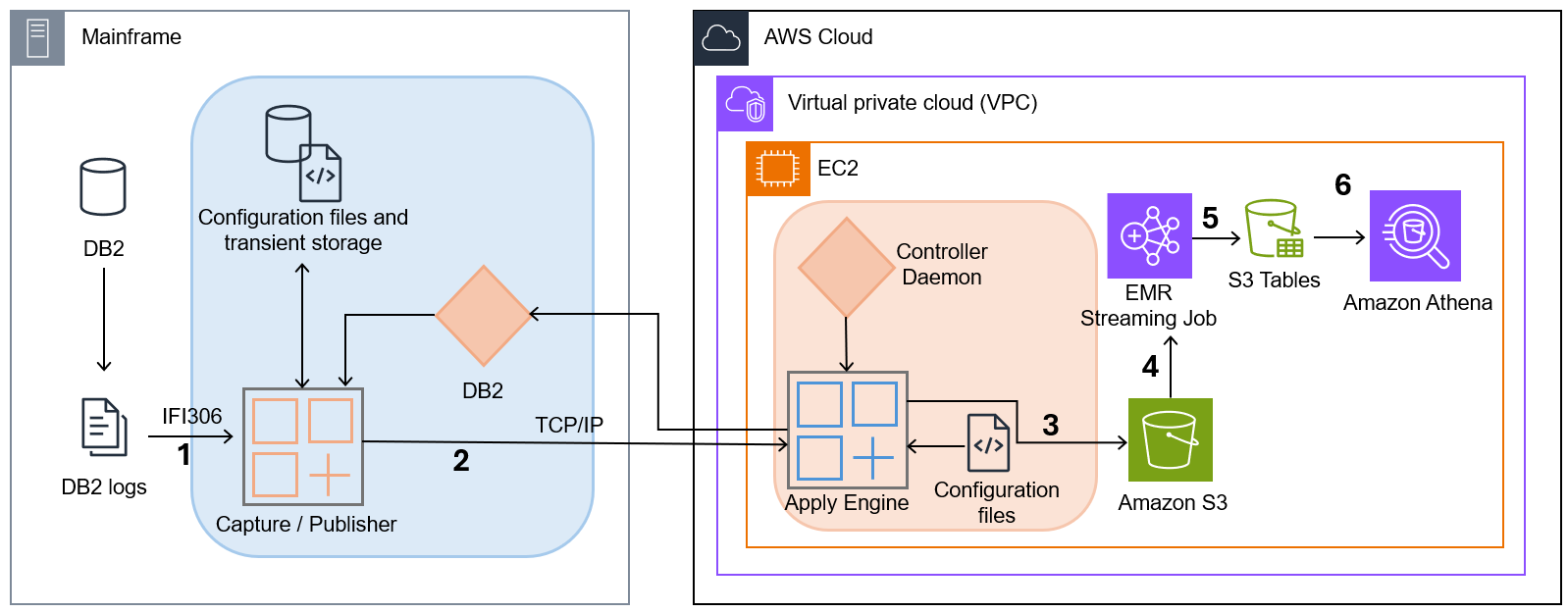
The following diagram illustrates the solution architecture.
Capture/Publisher – Connect CDC Capture/Publisher captures Db2 changes from Db2 logs using IFI 306 Read and communicates captured data changes to a target engine through TCP/IP.
Controller Daemon – The Controller Daemon authenticates all connection requests, managing secure communication between the source and target environments.
Apply Engine – The Apply Engine receives the changes from the Publisher agent and applies the changed data to the target Amazon S3.
Amazon S3 – Serves as the scalable data lake foundation where replicated mainframe data lands.
Amazon EMR streaming job – As data arrives, an instance of the Amazon EMR streaming job writes the data to target tables in Amazon S3 Tables.
Amazon Athena – Queries data stored in Amazon S3 Tables using standard SQL.
This architecture provides a clean separation between the data capture process and the data consumption process, allowing each to scale independently. When CDC data arrives in Amazon S3, you can use Amazon S3 Tables to store Db2 z/OS, VSAM, and IMS data in an open table format (Apache Iceberg) that is ready for analytics, providing a flexible path to mainframe modernization.
Quantifiable business value
Organizations implementing this solution typically see significant reductions in mainframe operational costs by offloading analytics and reporting workloads to the cloud. The elimination of intermediary infrastructure reduces both capital and operational expenses. The reduced maintenance burden frees IT resources to focus on strategic initiatives rather than managing complex replication systems. Speed and agility improvements are equally significant. Near real-time data availability, measured in seconds to minutes rather than hours to days, enables organizations to respond rapidly to market changes and operational events. The rapid deployment of new analytics use cases without requiring mainframe changes accelerates innovation. Organizations gain access to the full breadth of AWS services that can be used immediately after data lands in Amazon S3.
From an analytics and AI perspective, the solution creates a unified data platform that brings together mainframe, cloud-native, and third-party data sources. This unified view enables advanced machine learning on historical and current data, delivering predictive insights that drive proactive decision-making across the organization.
Customer story
A leading global payments provider put this into practice. The payments provider was struggling to generate timely analytics and insights from Point of Sale (POS) transaction data. As one of the world’s largest payment providers, they process hundreds of thousands of transactions per second. Users expect to swipe their card and have their transaction approved in seconds. New architecture was needed to keep up with customer demands and volume. By streaming mission-critical mainframe data directly to AWS in real time using Precisely Connect and landing it in Amazon S3 Tables, the company used storage built on the Apache Iceberg open standard. This approach enables high-performance analytics directly on mainframe data alongside cloud-native sources.
Conclusion
In this post, we demonstrated how Precisely Connect enables real-time, direct data replication from mainframes to Amazon S3, eliminating intermediaries and simplifying mainframe modernization.
Your organization can further extend this foundation with Amazon S3 Tables, purpose-built storage for Apache Iceberg tables in S3, enabling analytical applications to query the most current mainframe data using tools such as Amazon Athena, Amazon EMR, and Amazon Redshift.
Get started by deploying AWS Mainframe Modernization – Data Replication for IBM z/OS from AWS Marketplace and use Amazon S3 as a target for your mainframe use cases. Learn more about Precisely’s mainframe data integration capabilities at precisely.com. Contact AWS and Precisely experts to discuss your specific modernization challenges and design a proof-of-concept that demonstrates business value quickly.
The kernel’s DAMON subsystem
provides user-space monitoring and management of system memory. DAMON is
developing rapidly, so an update on its progress has become a regular
feature of the annual Linux Storage,
Filesystem, Memory Management, and BPF Summit. This tradition
continued at the 2026 gathering with an update from DAMON creator SeongJae
Park covering a long list of new capabilities — tiering, data attributes
monitoring, transparent huge pages, and more — being added to this subsystem.
Every engineering team in your organization ships code through a pipeline. They branch, test, review, and deploy. If something breaks, they roll back. If someone asks “what changed?”, the answer is in the commit history. This isn’t heroic discipline to process; it’s just how software gets built.
Now think about how your detection engineering team works.
Rules get written in a UI. Maybe copied and pasted from a wiki. There’s no peer review; someone clicks “save,” and it’s live. No test cases validate the logic before deployment. No rollback if something breaks. When an alert suddenly floods your SOC, good luck figuring out what changed and when. When a detection stops firing, you might not notice for weeks.
This is, by definition, a process gap. And it’s one that the rest of engineering solved years ago. The gap becomes manageable through the five custom rules, listed below. As your detections grow, you need the same discipline that every other engineering team already has.
Process Stage
How it works in software engineering
How it works in detection engineering
Storage
Git / Version Control
UI / Wiki / “Tribal Knowledge”
Validation
Automated CI/CD Tests
“Wait and see if it fires”
Review
Peer-reviewed Pull Requests
Single-user “Save” button
Rollback
One-click git revert
Manual query deletion
How does this help my security team?
Detection as Code gives your team a structured, repeatable way to build and manage detections with confidence. Instead of relying on manual updates and guesswork, every change is tested, reviewed, and tracked before it reaches production. Before we get into the how, here’s why Detection as Code changes the way your team works:
A more reliable process. Every change goes through version control and peer review before it goes live. When something goes wrong, you know exactly what changed, when it changed, and who approved it. Roll back in seconds if needed.
A safety net of tests. Inline test cases validate detection logic before deployment. Positive tests prove it catches the threat; negative tests prove it doesn’t fire on legitimate activity.
Confidence in what’s deployed.terraform plan previews every change before anything touches production. Terraform state is the authoritative record of your detection estate, not some spreadsheet.
The result is a detection workflow your team can trust. Changes are predictable, validated, and fully traceable, so security teams don’t get caught up in troubleshooting and can focus on improving coverage and overall posture.
The anatomy of a detection
Here is what a detection rule looks like using Rapid7’s Terraform provider. It offers a practical view of how detection engineering teams can use Detection as Code in practice:
Version-controlled logic: The LEQL query defines the threat logic in a text format that Git can track.
MITRE ATT&CK® untegration: The techniques field ensures your coverage map updates automatically.
Inline testing: We aren’t just deploying a query, but a validated unit of logic. The pipeline won’t let this reach production if the logic fails to fire on the matching” payload or accidentally fires on the un-matching payload.
Why Terraform?
Because it’s the industry standard for managing infrastructure as code. We didn’t invent a proprietary CLI; we built on the tool that thousands of platform teams already run daily. If your organization uses Terraform for cloud infrastructure, your detection engineers now use the same tool, the same workflow, and the same review process.
Governance happens naturally in this model. Open a pull request. Your team sees the logic, the test cases, and the expected behavior. They comment, suggest improvements, and approve. Every change is traceable in your commit history. This isn’t a separate compliance exercise bolted onto your workflow. It is the workflow.
Already have rules built in the UI? One command imports them all:
terraform query -generate-config-out imports.tf
AI-assisted detection writing
The quick-start repo ships with IDE configurations for Claude Code, Cursor, VS Code Copilot, and Kiro. These configs give your AI assistant full context on the Terraform provider schema, LEQL syntax, and MITRE ATT&CK mappings.
In practice: open your editor, describe a threat in plain English, such as ‘write me a detection for lateral movement via RDP from non-admin workstations,’ and get back a complete Terraform resource ready for review. The AI accelerates the engineer; it doesn’t replace them. The time from “I need a detection” to “this is ready for review” drops from hours to minutes.
Start building detections as code today
Rapid7’s Terraform provider for Detection as Code is now available across all Incident Command and InsightIDR tiers.
To get to work, use the Getting Started guide for a walkthrough as you setup, authenticate, and run your first deployment. Clone the quick-start template, run terraform plan, and see your detection estate as code. For more information on Incident Command, visit Our hub page for SIEM.
Greg Kroah-Hartman has announced the release of the 7.0.5, 6.18.28, 6.12.87, and 6.6.138 stable kernels. These kernels
contain a partial fix for the Dirty
Frag and Copy Fail 2
security flaws. Kroah-Hartman has confirmed
that a second patch is required, but it is still in development and has not yet been merged.
The collective thoughts of the interwebz
Manage Consent
To provide the best experiences, we use technologies like cookies to store and/or access device information. Consenting to these technologies will allow us to process data such as browsing behavior or unique IDs on this site. Not consenting or withdrawing consent, may adversely affect certain features and functions.
Functional
Always active
The technical storage or access is strictly necessary for the legitimate purpose of enabling the use of a specific service explicitly requested by the subscriber or user, or for the sole purpose of carrying out the transmission of a communication over an electronic communications network.
Preferences
The technical storage or access is necessary for the legitimate purpose of storing preferences that are not requested by the subscriber or user.
Statistics
The technical storage or access that is used exclusively for statistical purposes.The technical storage or access that is used exclusively for anonymous statistical purposes. Without a subpoena, voluntary compliance on the part of your Internet Service Provider, or additional records from a third party, information stored or retrieved for this purpose alone cannot usually be used to identify you.
Marketing
The technical storage or access is required to create user profiles to send advertising, or to track the user on a website or across several websites for similar marketing purposes.