Post Syndicated from The Atlantic original https://www.youtube.com/shorts/7dj7ZX80e4A
Understanding and optimizing materialized views in Amazon Redshift
Post Syndicated from Nick Barclay original https://aws.amazon.com/blogs/big-data/understanding-and-optimizing-materialized-views-in-amazon-redshift/
Analytical queries often repeat the same expensive joins and aggregations, and materialized views (MVs) in Amazon Redshift optimize that pattern. An MV pre-computes and stores a query’s result, so the expensive work happens at refresh time instead of on every read. A query that would otherwise scan and aggregate large tables becomes a fast lookup of the stored result.
That speed has a running cost. Every MV consumes storage, and every refresh consumes compute, whether or not a query ever reads the result. A well-used MV repays that cost many times over. An MV that refreshes constantly but is not read costs more than it saves. So does one that fully recomputes a hundred million rows to serve a handful of queries.
As MVs become more popular in your organization, it can be challenging to keep track of which MVs are worth the maintenance costs. This post introduces a diagnostic view, v_mv_health, that reports each MV’s refresh eligibility, staleness, refresh cost, dependencies, and query activity. A companion stored procedure, sp_populate_mv_definitions(), creates and fills a table, mv_definitions, holding the one signal a view cannot compute. It reads each MV’s definition and flags the SQL constructs that block incremental refresh. Join the two for a single result set that covers these signals. Once deployed, the view and procedure give you the data to make MV health part of your regular operational review.
Solution overview
The following diagram shows how the two components fit together.
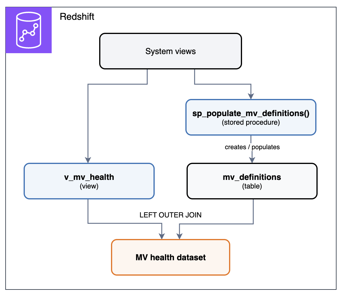
Figure 1: How the v_mv_health view and sp_populate_mv_definitions procedure combine into the MV health dataset
Both components read from Amazon Redshift system views. The v_mv_health view reads them directly each time you query it. The sp_populate_mv_definitions() procedure reads each MV’s definition, flags constructs that block incremental refresh, and writes the results to the mv_definitions table each time it runs. Joining v_mv_health with mv_definitions produces the MV health dataset, a single result set with one row per MV.
Prerequisites
The diagnostic view and procedure require:
- An Amazon Redshift provisioned cluster or an Amazon Redshift Serverless workgroup with one or more MVs.
sys:superuserrole, or thesys:monitorrole, so the view can read activity in the cluster or workgroup. Without it, the refresh and query activity the view reports covers only your own sessions. Grant it withGRANT ROLE sys:monitor TO <username>;(for an IAM identity, use theIAMR:role-nameform). For the full list of system-defined roles, refer to Amazon Redshift system-defined roles.- For a non-superuser (such as a
sys:monitoruser),USAGEon each schema that contains MVs, becauseSVV_MV_INFOonly returns MVs in schemas the user can access. Grant it withGRANT USAGE ON SCHEMA <schema> TO <username>;.
The diagnostic view
Amazon Redshift already exposes the signals, but each lives in a different system view:
- State and staleness: SVV_MV_INFO (current state, staleness, autorefresh setting, and interval).
- Dependencies: SVV_MV_DEPENDENCY (MV-on-MV relationships).
- Refresh history: SYS_MV_REFRESH_HISTORY (refresh activity, method, duration).
- Query activity: SYS_QUERY_DETAIL and SYS_QUERY_HISTORY (which MVs are actually being read, including through automatic query rewriting).
The v_mv_health view joins them into a single row per MV: state, staleness, autorefresh interval, refresh cost, query activity, dependency depth, and whether parent MVs in a chain are stale. The definition for the v_mv_health view is available in the amazon-redshift-utils GitHub repository.
The stored procedure
One signal the view can’t provide is the MV’s definition text. The sp_populate_mv_definitions() procedure iterates through each MV and extracts its definition into the mv_definitions table, created automatically if it doesn’t exist. It then scans each definition for SQL constructs covered in Refresh eligibility. The definition for the sp_populate_mv_definitions() procedure is available in the amazon-redshift-udfs GitHub repository.
The procedure uses a two-phase approach: it stages the MV object IDs into a temporary table first, then walks that local table one row at a time. It executes the pg_get_viewdef() function, which operates on one view at a time. Results are collected in a second temporary table and then replace the contents of mv_definitions in a single transaction, so each run reflects the current state of your MVs. Amazon Redshift drops the temporary tables automatically at the end of the session, so no manual cleanup is needed.
Run the procedure, then join the v_mv_health view to the mv_definitions table it populated:
Both objects use the same SQL on provisioned clusters and serverless workgroups. They report the MVs in their own database, so create them in each database that contains MVs.
Note: The view uses a 7-day lookback window because SYS_MV_REFRESH_HISTORY, SYS_QUERY_DETAIL, and SYS_QUERY_HISTORY retain 7 days of data by default. Amazon Redshift can retain system table data beyond 7 days by automatically replicating it to Amazon S3 Tables, a capability of Amazon Simple Storage Service (Amazon S3). Long-term retention supports SYS_QUERY_HISTORY and SYS_QUERY_DETAIL, so you can extend the query-activity signals by pointing the view’s queries on them at the retained tables. At the time of writing, SYS_MV_REFRESH_HISTORY is not among the retained system tables, so the refresh-cost columns remain limited to the 7-day in-cluster window unless you capture that history yourself.
What the output tells you
The joined output returns one row per MV:
| Column | What it means |
mv_database |
Database containing the MV |
mv_schema |
Schema containing the MV |
mv_name |
MV name |
state |
1 (incremental), 0 (full_recompute), 101-105 (broken). Refer to SVV_MV_INFO |
state_label |
incremental, full_recompute, or broken with its cause (for example, broken:column_renamed) |
is_stale |
Whether MV data is out of date relative to base tables; NULL for MVs on external tables other than Iceberg. |
is_autorefresh |
Whether automatic refresh is turned on |
autorefresh_interval_sec |
Autorefresh interval in seconds; NULL when autorefresh is off |
is_default_autorefresh_interval |
Whether the MV uses the cluster or workgroup default interval rather than its own. false when autorefresh is off |
is_autorewrite_eligible |
Whether the optimizer can transparently rewrite queries to use this MV |
refresh_count |
Refresh attempts in the last 7 days, including failed refreshes and refreshes that found the MV already up to date |
query_count |
Queries that read the MV in the last 7 days, including queries served through automatic query rewriting. Refreshes are excluded; NULL if the MV’s storage table can’t be found in the catalog |
recompute_to_query_ratio |
Full-recompute refreshes (not incremental) ÷ queries. High values indicate refresh cost may exceed benefit; NULL when query_count is 0 or NULL |
avg_refresh_sec |
Average refresh duration in seconds |
last_refresh_status |
Status message from the most recent refresh, such as incremental, full recompute, or already up to date |
mv_rows |
Row count of the MV, for gauging refresh cost against usage |
chain_depth |
Depth in a dependency chain (0 = no MV dependencies) |
mv_dependencies |
Parent MVs the MV depends on; NULL if it has no parent MVs |
stale_ancestors |
Parent MVs in the chain that are currently stale; NULL if no parent MV is stale |
pct_of_total_query_time |
Refresh time as a percentage of total query time on the cluster or workgroup |
incremental_blocker_hint |
SQL constructs preventing incremental refresh, evaluated only for state 0 MVs (none otherwise, unidentified when no known construct matches). From mv_definitions |
Refresh eligibility
Amazon Redshift refreshes an MV in one of two ways. In an incremental refresh, Amazon Redshift identifies the changes to the data in the base tables since the last refresh and updates the data in the MV. In a full recompute, it reruns the MV definition, replacing the data in the MV. Amazon Redshift automatically chooses the method based on the query that defines the MV.
Each MV in Amazon Redshift falls into one of three states:
- Full recompute (state 0): The entire MV is rebuilt from scratch on every refresh.
- Incremental (state 1): Only changed rows are processed on refresh.
- Broken (state 101-105): The MV cannot refresh at all and must be dropped and recreated.
The state column tells you which category each MV falls into. An MV’s state depends on its definition, not its size. Its size (mv_rows) determines how much that state costs. An incremental refresh on a 100-million-row table might process 50 changed rows, while a full recompute scans all 100 million regardless of how few changed.
Note: A state 1 MV can still occasionally fully recompute, for example after a VACUUM with the FORCE option on a base table while the MV is out of date, or when the MV hasn’t been refreshed for an extended period. These show up as full recomputes in recompute_to_query_ratio even though the state is 1. If you need VACUUM FORCE, run it straight after refreshing the dependent MVs.
Certain SQL constructs block incremental refresh. The incremental_blocker_hint column identifies which constructs are preventing incremental eligibility. If any of the following appear in the MV definition, the MV cannot refresh incrementally and falls back to a full recompute on every refresh:
- Distinct:
SELECT DISTINCT,COUNT(DISTINCT ...). - Outer joins:
LEFT,RIGHT, orFULL OUTER JOIN. - Window functions: anything with an
OVER()clause (ROW_NUMBER,RANK,SUM,NTILE, and so on). - Subqueries: in the
WHEREclause orSELECTlist (subqueries in theFROMclause are fine). - Mutable functions:
GETDATE(),SYSDATE,RANDOM(),CURRENT_DATE. - Set operations:
UNION,INTERSECT,EXCEPT,MINUS. - Ordered and holistic aggregates:
MEDIAN,PERCENTILE_CONT,PERCENTILE_DISC,LISTAGG,APPROXIMATE COUNT,APPROXIMATE PERCENTILE.
An MV may trip more than one of these at once, and incremental_blocker_hint lists each one it finds.
Note: incremental_blocker_hint is a heuristic text scan of the MV definition, not a semantic parse, and is evaluated only for MVs in state 0. The other MVs show none. It matches whole-word SQL keywords, so it won’t trip on names like distinct_count, but a keyword inside a string literal (for example, WHERE status = 'union') can still produce a false positive. Treat it as guidance and verify by inspecting the definition.
OUTER JOIN is a frequent blocker. Outer joins (FULL, LEFT, and RIGHT) are a legitimate and important SQL pattern, but they prevent incremental refresh in MVs. If you need incremental eligibility, you have options: if the join always produces a match (no NULLs in the result), rewriting as INNER JOIN restores incremental refresh with no change to output. If the outer join is genuinely needed, consider handling the unmatched rows upstream. For example, pre-joining in an ETL step, or using a regular view for the outer join while keeping the MV incremental on the inner-joined subset.
For the full list of incremental refresh limitations, refer to Refreshing a materialized view in the Amazon Redshift documentation.
Refresh cost
Every refresh consumes compute resources. The pct_of_total_query_time column shows what share of total query time is spent refreshing each MV, and avg_refresh_sec identifies individual MVs with unusually long refresh times. There is no universal threshold, because what counts as expensive depends on the cluster. Start with the MVs that rank highest on pct_of_total_query_time: those in the highest decile of refresh cost, and those whose cost looks large relative to the queries they serve.
The net-negative MV. An MV that refreshes frequently but is never queried consumes resources without delivering value: refresh_count > 0 with query_count = 0. If is_autorefresh = true and query_count = 0, consider dropping the MV. If it’s still needed occasionally, lengthen its autorefresh interval or switch it to manual refresh on demand.
Refresh-to-query ratio. Even when queried, the refresh cost may exceed the benefit. If an MV fully recomputes many times for every query that reads it, the caching isn’t paying for itself. The recompute_to_query_ratio column flags this. Consider lengthening the autorefresh interval or scheduling refreshes to match how often the MV is read, or dropping the MV entirely.
Note: Amazon Redshift supports creating an MV on a consumer warehouse over data-shared base tables or directly refreshing an MV from a remote warehouse. This isolates the compute and minimizes cluster disruption, whether the refresh is full or incremental.
Dependencies and staleness
Amazon Redshift supports MVs that reference other MVs, known as nested MVs. Nested MVs can be refreshed together, in dependency order, using REFRESH ... CASCADE (refer to Harnessing the power of nested materialized views and exploring cascading refresh). The chain_depth column shows how deep each MV sits in a dependency tree, and mv_dependencies lists its parent MVs.
Staleness propagates one hop at a time. The is_stale column reports whether an MV’s data is behind its base tables. When base table data changes, the immediate dependent MV is marked is_stale = true. Downstream MVs remain is_stale = false until their direct parent is refreshed. At that point they become stale in turn. For deeper chains, is_stale = false on a downstream MV indicates freshness relative to its immediate parent, not the original base table. The stale_ancestors column walks the full chain and reports which parent MVs are currently stale.
CASCADE refresh solves propagation but requires explicit invocation. REFRESH MATERIALIZED VIEW mv_name CASCADE refreshes the entire chain in topological order (parent MVs first). It is not automatic and autorefresh does not cascade, so run it at your required freshness interval, for example on a schedule with Amazon EventBridge and the Amazon Redshift Data API, or as the final step of the ETL job that loads the base tables. Refer to the Autorefresh section for details on when AUTO REFRESH YES is supported.
Note: CASCADE is supported only for chains built on local tables, data-shared tables, local MVs, and streaming MVs. It doesn’t extend to MVs on Amazon Redshift Spectrum sources or to MVs shared from another warehouse, which must be refreshed individually in dependency order. Each additional level in a dependency chain adds refresh latency and widens the window where downstream MVs serve data that hasn’t caught up. Keep chains shallow, and weigh that lag against the benefit the chain provides.
Refreshing materialized views on external tables
MVs can cache results from external tables stored in Amazon S3, so each query reads the stored result instead of re-scanning the same Amazon S3 files. Refresh behavior depends on two factors:
- Data storage format: a standard file type (Parquet, CSV, Avro) or an open table format (Apache Iceberg, Hudi, Delta Lake). When new files appear in Amazon S3, MVs on standard file types and Iceberg refresh incrementally, whether or not they aggregate. Hudi and Delta Lake don’t support incremental refresh.
- Aggregation: whether the MV aggregates (
GROUP BY,SUM,COUNT). When a file is deleted or overwritten, a non-aggregating MV stays incremental, but an aggregating MV must fully recompute, because aggregates can’t be undone without re-reading the remaining data. Thelast_refresh_statuscolumn reports this as “A full recompute was successfully completed as a data file was deleted.”
Apache Iceberg supports incremental refresh in more cases than the other formats. Iceberg’s metadata layer tracks row-level changes (inserts, deletes, updates, compaction), so aggregating MVs stay incremental even when rows are removed. Iceberg is the only data lake format that accepts AUTO REFRESH YES. For MVs over data lake sources where incremental refresh matters, Iceberg is the strongest fit (refer to materialized views on external data lake tables). For a deeper treatment of how incremental refresh works across data lake table formats, refer to Incremental refresh for Amazon Redshift materialized views on data lake tables.
Note: An incrementally refreshable materialized view on Iceberg tables may fall back to a full recompute if that is expected to perform better, or if it joins multiple base tables and more than one of them has been updated since the last refresh.
The following table summarizes the refresh method each source format uses for file additions and deletions, and whether it supports autorefresh:
| Source format | On file addition | On file deletion, non-aggregating MV | On file deletion, aggregating MV | Autorefresh |
| Apache Iceberg | Incremental | Incremental | Incremental | Supported |
| Parquet / CSV / Avro | Incremental | Incremental | Full recompute | Not supported |
| Hudi / Delta Lake | Full recompute | Full recompute | Full recompute | Not supported |
Note: On Iceberg tables, an aggregating MV falls back to a full recompute if a snapshot it needs has been expired. Expire snapshots only after refreshing the MVs that depend on the table, and if you use AWS Glue Data Catalog snapshot retention, keep the retention period longer than the interval between MV refreshes. Refresh after compaction stays incremental but processes more data, so plan for a longer refresh.
On Amazon Redshift RG instances and Serverless, external table queries run through an integrated query engine rather than Amazon Redshift Spectrum, which can reduce MV refresh times on Iceberg data. No configuration change is required.
Autorefresh
Autorefresh keeps MVs current without manual scheduling. The is_autorefresh column shows which MVs have it turned on, and autorefresh_interval_sec shows how often Amazon Redshift checks each one for staleness. An autorefresh runs only when the MV is stale, with the same priority as other user queries. On provisioned clusters, autorefresh queries run in your workload management (WLM) queues alongside your workload and appear in STL_QUERY. On Amazon Redshift Serverless, they consume Redshift Processing Units (RPUs) like any other query. On both, SYS_MV_REFRESH_HISTORY is where you see autorefresh activity, because it doesn’t appear in SYS_QUERY_HISTORY.
Autorefresh on high-churn tables generates constant refresh activity. Some base tables change frequently through streaming ingestion, AWS Database Migration Service (AWS DMS) replication, or zero-ETL. On those tables the MV is almost always stale, so autorefresh runs at every interval (5 minutes by default). The refresh_count column quantifies this. The worst case is autorefresh on a state 0 MV. Every refresh is a full recompute, so at the default interval that’s a full rebuild of the MV every 5 minutes. If the MV doesn’t need to be that current, keep autorefresh on but lengthen the interval (minimum 60 seconds) to match how often the results are queried: ALTER MATERIALIZED VIEW mv_name AUTO REFRESH YES INTERVAL <seconds>. To change the default for every MV on the cluster or workgroup, use ALTER SYSTEM SET default_mv_auto_refresh_interval = <seconds>. For details, refer to ALTER MATERIALIZED VIEW and ALTER SYSTEM. Custom intervals aren’t supported on streaming MVs.
Autorefresh does not cascade. It refreshes only the configured MV, not its dependents. AUTO REFRESH YES is rejected at creation time on nested MVs and on external tables other than Iceberg, returning an error rather than being silently ignored. On a nested MV the message is “Auto-refresh is not supported for materialized views defined on other materialized views.” It is supported on local single-level MVs over Iceberg or datashare tables, but not on an MV that combines both.
Broken materialized views
An MV becomes permanently broken when the definition of its base table changes in certain ways. The state column shows values 101-105 for broken MVs, with a label indicating the cause (refer to SVV_MV_INFO for the full state code reference).
Renaming an object that an MV depends on is not blocked, and it leaves the MV unable to refresh. A rename of a column, table, or schema completes without an error and moves the MVs that reference it to a broken state (103-105). Once broken, an MV cannot be refreshed, and renaming the object back does not restore it. The fix is to DROP and CREATE the MV.
Dropping a column that an MV uses, or changing its data type, is rejected. Amazon Redshift returns an error and the MV stays healthy.
Identify affected MVs before you alter a base table or column. SVV_MV_DEPENDENCY only shows MV-on-MV relationships, not base-table dependents. Before you make such a change, use the v_view_table_column_dependency view in the amazon-redshift-utils GitHub repository to identify the dependent MVs and the specific columns they rely on.
Automatic query rewriting
Amazon Redshift can rewrite a query on base tables to read from an MV, even when the query doesn’t name it (refer to Automatic query rewriting to use materialized views). The query_count column includes these reads. The is_autorewrite_eligible column shows whether the MV’s definition allows rewriting.
Eligible doesn’t mean used. Amazon Redshift skips a stale MV until its next refresh, even though the flag stays true. The flag also reads true for nested and broken MVs, which aren’t used. To confirm a specific query was rewritten, run EXPLAIN on it. In a rewritten plan, the base tables the MV covers no longer appear. In their place is a scan of an internal table that holds the MV’s results.
Should this be a materialized view?
Not every cached result benefits from being an MV. The following characteristics indicate when an MV is a strong fit and when an alternative is likely better:
| Favors a materialized view | Points to an alternative |
| Analytical queries from dashboards and analysts | Application lookups serving thousands of concurrent requests |
| Multiple users or queries read the result | The result is read once or rarely |
| The query scans a large table but returns few rows | The query returns most of the rows it scans |
| Query latency is unacceptable without pre-computation | A regular view already meets the latency requirement |
| Readers can tolerate data that is a refresh interval old | Readers need sub-minute freshness |
When your workload matches the right-hand column, a different approach usually fits better: a regular view when the query is already fast enough, in-stream transformation when readers need sub-minute freshness, and an in-memory cache such as Amazon ElastiCache for application lookups at high concurrency.
Putting it together
Deploy the diagnostic view and stored procedure. Run them periodically. Weekly is sufficient for most clusters. Focus on:
- State 0 MVs with high refresh cost: Check
incremental_blocker_hint. If it names an SQL construct, refactor it (for example,OUTER JOINtoINNER JOIN). If it readsunidentified, confirm the full recompute is justified. - MVs with
query_count = 0: Consider dropping them. - Deep chains with stale ancestors: Refresh with
REFRESH ... CASCADEto bring the chain current, and flatten chains that are deeper than they need to be. - Broken MVs (state 101-105): Drop and recreate.
- Autorefresh MVs on high-churn tables: Compare
refresh_countagainstquery_count. When refreshes far outnumber reads, lengthen the autorefresh interval to match how often the results are actually queried.
The goal is MVs whose refresh cost is repaid by the queries they accelerate.
Automate the review. Rather than running the diagnostic by hand, schedule it. v_mv_health is consistently current because it reads the system views each time you query it, so only the procedure needs a schedule. For a basic setup, run CALL sp_populate_mv_definitions(); on a cadence with Amazon EventBridge and the Amazon Redshift Data API. For alerting or dashboards, refer to Building an event-driven application with AWS Lambda and the Amazon Redshift Data API, which uses Amazon EventBridge and AWS Lambda to run a stored procedure on a schedule.
Cleaning up
The diagnostic objects are lightweight (a view, a stored procedure, and a small definitions table), but if you no longer need them, remove them with:
Summary
In this post, we showed how to check the health of the MVs in an Amazon Redshift database from a single result set. The v_mv_health view and the sp_populate_mv_definitions() procedure surface the signals that matter. Together they cover refresh eligibility, cost, staleness, dependencies, broken states, and autorefresh behavior. Call the procedure, join its output to the view, and you can see which MVs need attention first.
With v_mv_health and sp_populate_mv_definitions() deployed in each database that contains MVs, you can make MV health a routine part of your operational reviews.
Next steps. The v_mv_health and v_view_table_column_dependency views are available in the amazon-redshift-utils GitHub repository, and the sp_populate_mv_definitions() procedure is available in the amazon-redshift-udfs GitHub repository. To go deeper on the topics this post touched, see Harnessing the power of nested materialized views and exploring cascading refresh and Incremental refresh for Amazon Redshift materialized views on data lake tables.
About the author
Handling large volume of transactions with AWS Lambda Managed Instances
Post Syndicated from Mythili Annamalai Sekar original https://aws.amazon.com/blogs/compute/handling-large-volume-of-transactions-with-aws-lambda-managed-instances/
Pre-scheduled events like concert ticket on-sales and product launches can drive a load spike 100 times higher than the baseline. The spike persists for a few hours while the inventory clears, then traffic returns to normal. If you miss the first minute of the on-sales, customers experience errors while competitors keep selling, and the event’s reputation takes a hit. Over-provision for the burst, and you pay for peak capacity 24 hours a day, 365 days a year. The actual peak lasts 10 minutes and happens 10 times a year.
In this post, you will see how AWS Lambda Managed Instances, a capability of AWS Lambda, handles predictable traffic bursts. It keeps compute capacity warm before the on-sales event opens and scales it back down afterward. You will see a reference ticketing implementation that sustains 40,000 transactions per second (TPS) for 120 seconds.
Understanding Lambda Managed Instances
Lambda Managed Instances runs your Lambda functions on Amazon Elastic Compute Cloud (EC2) instances in your account, including Graviton4 and memory-optimized instance types. AWS handles the underlying infrastructure lifecycle (provisioning, scaling, patching, and routing), while you benefit from EC2 pricing including Compute Savings Plans and Reserved Instances.
Lambda Managed Instances provides several benefits. With pre-provisioned execution environments (EE), capacity is already warm before traffic arrives, so there are no cold starts when a burst hits. Scaling bounds are configurable with MinExecutionEnvironments and MaxExecutionEnvironments for each function, and each new EE comes online in 1–2 seconds. With multi-concurrent invocations, one EE handles multiple requests at once, which improves utilization for I/O-heavy handlers. You also get EC2 pricing, so Compute Savings Plans and Reserved Instances apply instead of per-request Lambda pricing.
Lambda Managed Instances is well suited for predictable, spike-shaped workloads that need sustained compute capacity during the peak and can scale back down when traffic returns to the baseline.
Predictable burst workloads work best with Lambda Managed Instances
This post focuses on one of the key capabilities of Lambda Managed Instances: absorbing scheduled traffic bursts without provisioning for peak year-round. Some of the use cases where Lambda Managed Instances helps are ticket and event on-sales (concerts, sports, festivals), live streaming and voting events, and scheduled batch and report generation nightly or hourly jobs that consume steady compute during a defined window.
Use case: High-throughput ticket booking with Lambda Managed Instances
To demonstrate Lambda Managed Instances handling predictable traffic bursts, we built a concert ticketing backend. The solution implements the industry-standard queue-plus-hold-and-confirm booking flow, a pattern that ticketing platforms, airlines, and hotels use to prevent overselling during large traffic spikes. It separates user traffic management from the critical database transactions required to lock inventory.
The following diagram presents the detailed architecture of the solution we built.
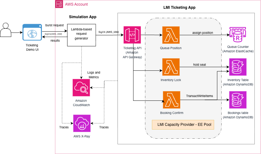
Figure 1: Architecture of the concert ticketing solution across two AWS CloudFormation stacks
The solution deploys two AWS CloudFormation stacks in a single AWS Region. In the first stack, Amazon API Gateway routes public HTTPS traffic through three ticketing handlers hosted in Lambda Managed Instances on a shared capacity provider. Amazon ElastiCache Serverless for Valkey holds the atomic queue counter. Amazon DynamoDB holds durable per-seat state across a write-sharded inventory table (500 shards) and a bookings table. WarmThroughput is pre-provisioned to absorb the burst without waiting for adaptive capacity. A separate simulation stack drives synthetic load through a three-tier Lambda fan-out, reproducing the on-sales burst shape at any target TPS.
Public traffic and load-generation traffic take completely separate code paths, so the load generator’s own scaling behavior does not affect measurements on the ticketing stack. Each successful booking traverses three Lambda handlers. Handler queue-position assigns an atomic virtual queue number using an INCR on a single ElastiCache key. Handler inventory-lock places a time-bounded hold on a specific seat through a DynamoDB conditional UpdateItem, moving it from AVAILABLE to HELD with a time to live (TTL) of 180 seconds. Handler booking-confirm executes a single TransactWriteItems call that atomically transitions the seat from HELD to CONFIRMED and writes a durable booking record. Either both writes succeed or neither does.
All three handlers are stateless, because each request they receive is treated as an independent, standalone transaction. The mutable state lives in ElastiCache and DynamoDB, stored with safety features like conditional writes and atomic operations to avoid collisions, race conditions, and overwrites. This is why the multi-concurrent EE model of Lambda Managed Instances can serve thousands of simultaneous invocations per instance safely.
What makes this solution better with Lambda Managed Instances
With Lambda Managed Instances, you keep the same Lambda programming model, one function per handler, and the same deployment story, while Lambda Managed Instances handles the fleet. Raise MinExecutionEnvironments a few minutes before an on-sales opens, let it burst inside the Min to Max range while traffic is live, and scale back down when the window closes.
Deploy the application
For the full deployment instructions, refer to the README file in the GitHub repository after you have cloned it.
Prerequisites
- AWS Command Line Interface (CLI) version 2 configured with credentials.
- AWS Serverless Application Model (SAM) CLI installed.
- Python 3.13+ with
boto3installed. - An existing Amazon Virtual Private Cloud (VPC) with at least two subnets in different Availability Zones, plus either a NAT Gateway or VPC endpoints for DynamoDB and Amazon CloudWatch Logs.
- AWS Service Quotas – the initial deployment works with an AWS account’s default service quota. Peak-load testing requires EC2 vCPU and API Gateway throttle quotas increase.
Run the application
Once deployed, all test traffic goes through the simulation API. The sample includes an optional single-page web user interface (UI) (see the demo-ui/ folder in the repository) that wraps the same endpoints and renders the per-burst results interactively.
Read the “Cost considerations” section before running a simulation to understand the cost you will incur in the process.
1. Smoke test – low TPS to verify the pipeline end-to-end:
By default, deploy.sh provisions a cost-safe baseline of three warm EEs (Min=1, Max=3 per handler). The following smoke test works on this baseline.
2. Peak-load test
To reproduce the headline result, scale the Lambda handlers to the per-handler Min and Max values before firing the peak-load test. Refer to the Peak-load testing section of the GitHub repository before firing the burst. This also requires an EC2 vCPU and an API Gateway account-throttle quotas increase above the default.
3. View results
The response includes total requests, total bookings written to DynamoDB, delivered peak TPS, and end-to-end latency percentiles.
Interactive demo UI
The sample repository ships an optional single-page web UI (in the demo-ui/ folder) that wraps the same simulation and dashboard endpoints as the preceding curl examples. Point it at your simulation API endpoint, then fire bursts and view results interactively without leaving the browser.
Configure and start the UI:
Fire a burst. Choose a target load (a preset button or a custom TPS value), set the sustain duration and ramp, then choose Start burst. The UI sends a POST request to /simulation/start and stores the returned run_id and event_id, so you can query DynamoDB directly if you want to drill deeper.
View results. After the burst completes, choose View results. The UI queries API Gateway metrics, DynamoDB, CloudWatch Logs Insights, and CloudWatch Lambda metrics in parallel to reconstruct the run: total requests received, durable bookings written, and a per-handler table showing EEs used, Lambda throttles, and p95/p99 latency.
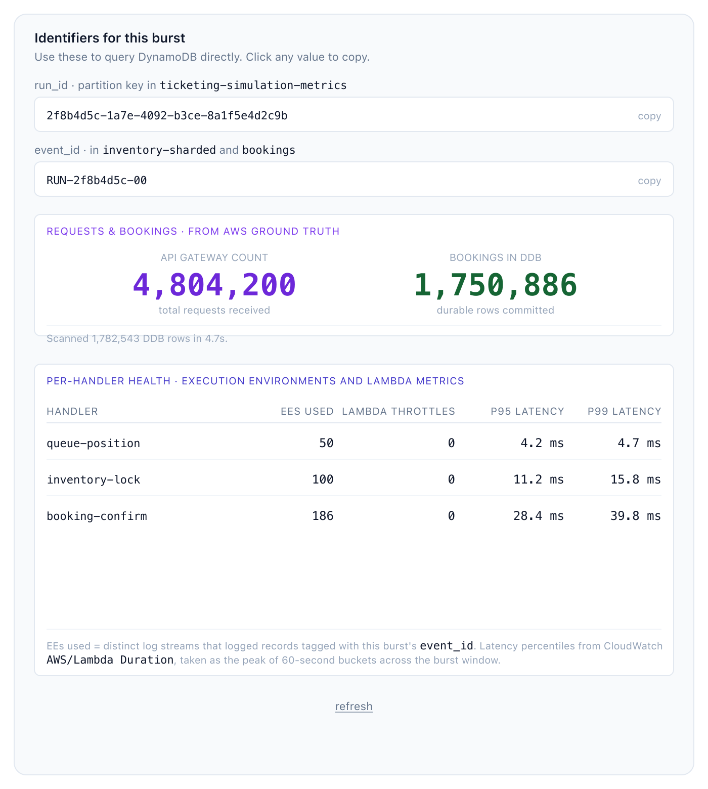
Figure 2: Demo UI results panel from a 40,000 TPS, 120-second run
The panel shows 4,804,200 API Gateway requests and 1,750,886 durable bookings, plus a per-handler table with the baseline EE pool (50/100/150 for queue-position, inventory-lock, and booking-confirm). During the burst, 36 additional EEs are pre-emptively warmed on booking-confirm, with zero Lambda throttles and p99 latencies of 4.7, 15.8, and 39.8 ms.
The identifiers panel at the top exposes the burst’s run_id (the partition key in the simulation metrics table) and event_id (used in both the inventory and bookings tables), so you can locate them directly in DynamoDB or CloudWatch Logs Insights for the specific burst you ran.
What we measured
Across a load range from 5,000 to 40,000 requests per second, the pre-warmed EE pool served every burst without cold-start impact. Key results from the headline 40,000 TPS × 120-second burst:
| Metric | Value |
| Delivered peak throughput | 40,035 req/sec |
| Total HTTP requests | 4,804,200 |
| Durable bookings written to Amazon DynamoDB | 1,750,886 |
| End-to-end p50 / p99 latency | 44 ms / 121 ms |
| AWS Lambda errors | 0 |
| AWS Lambda concurrency throttles | 0 |
| Amazon DynamoDB write throttles | 0 |
The tested range spanned 5,000 to 40,000 requests per second, an 8× spread in delivered load. Across it, p99 latency stayed within a 3 ms band. Doubling sustained throughput from 20,000 to 40,000 requests per second held at exactly 121 ms, which confirms that the pre-warmed pool had substantial headroom throughout the tested range.
Observability
Lambda Managed Instances automatically publishes metrics to CloudWatch and structured logs to CloudWatch Logs, giving you visibility into function performance and capacity utilization without additional code. During a burst, the metrics that matter most are:
- Duration percentiles per handler to confirm p99 latency stays flat as load rises.
- ConcurrencyThrottles to detect if any handler hits its
MaxExecutionEnvironmentsceiling. - Errors for handler-side failures.
- EE count (log-derived) to observe how quickly Lambda Managed Instances adds warm capacity above
Min.
The sample repository includes a demo dashboard endpoint that queries CloudWatch metrics, CloudWatch Logs Insights, and DynamoDB in parallel to reconstruct a per-burst report, API Gateway request count, durable bookings landed, distinct EEs used, and per-handler latency percentiles. Reconciling the simulation-side counts against the AWS ground truth catches load-generator artifacts and confirms the system-under-test numbers.
Cost considerations
Lambda Managed Instances uses EC2 instance pricing plus a 15% management fee. Compute Savings Plans and Reserved Instances apply to the underlying instance cost.
The Lambda Managed Instances configuration runs a small always-on baseline and uses a scaling script to pre-warm to 50/100/150 EEs in the minutes leading up to each event, then scales back down to baseline afterward.
To simulate a peak load under controlled conditions, the fleet is pre-warmed for a 7-minute window (5-minute ramp and 2-minute burst) then scaled back down. The cost breakdown can be as follows.
| Component | Volume | Rate | Cost |
| API Gateway requests | 4.8 M | $3.50 per 1 M | $16.80 |
| DynamoDB writes | 8.8 M WCU | $1.25 per 1 M | $11.00 |
| Lambda Managed Instances compute (peak window) | 75 × c7i.4xlarge × 7 min | $0.821 / instance-hr | $7.18 |
| Lambda Managed Instances request charges | 4.8 M | $0.20 per 1 M | $0.96 |
| CloudWatch Logs (~2 GB) | ingestion | $0.50 per GB | $1.00 |
| Amazon ElastiCache Serverless for Valkey | 4.8 M INCR operations |
ECPU-based | $0.30 |
| Total per burst | ~$37.00 |
The estimated cost for simulating each burst is around $37.
Best practices
Based on experience building this solution, here are key recommendations:
- Pre-warm before scheduled events. Raise
MinExecutionEnvironmentsusing an Amazon EventBridge Scheduler rule or a manual scaling script when you expect major spikes, giving Lambda Managed Instances enough time to scale the underlying instances. Restore the low baseline after the event. - Set MaxExecutionEnvironments aggressively. Lambda Managed Instances adds new EEs to your capacity provider. A high
MaxExecutionEnvironmentsvalue costs nothing while idle but absorbs unexpected demand during the burst. - Write-shard hot DynamoDB tables. For workloads writing thousands of items per second to one logical entity (a single event, a single product SKU), spread writes across a synthetic sharded partition key. This sample uses 500 shards per event.
- Use WarmThroughput on DynamoDB tables. Pre-provision physical partitions before the burst rather than waiting for adaptive capacity to expand during the first minute of the on-sales.
- Keep hot atomic counters out of DynamoDB. Single-row atomic increments in DynamoDB cap at approximately 1,000 operations per second.
- Make write endpoints idempotent. The sample uses a caller-provided
booking_idon the confirmation endpoint so that retries produce the same booking record instead of duplicates.
Clean up
When you are done exploring the solution, remove the provisioned resources to avoid ongoing charges. For the full cleanup commands and exact steps, refer to the GitHub repository README file.
Conclusion
Lambda Managed Instances brings the same Lambda programming model to workloads that need sustained, pre-provisioned compute during predictable bursts: ticket on-sales, product launches, registration windows, and other scheduled surge patterns. The concert ticketing example shows how a queue-plus-hold-and-confirm pattern built on Lambda Managed Instances can sustain 40,000 requests per second while costing less than an always-on EC2 fleet sized for the same peak.
Explore the Lambda Managed Instances documentation and try building your own predictable-burst serverless application. You can find the complete code for this example in the GitHub repository.
About the authors
Introducing the new AWS WAF security analytics dashboard
Post Syndicated from Praveen Hosur Narayana Gupta original https://aws.amazon.com/blogs/security/introducing-the-new-aws-waf-security-analytics-dashboard/
When blocked requests spike or a customer reports being locked out, a security team has to work out what is happening, where it is happening, and if AWS WAF is making the right call. Currently, that usually means opening each protection pack (web ACL) in turn, across domains, AWS Regions, and Amazon CloudFront distributions, or querying AWS WAF logs. In 2024, we introduced the AWS WAF traffic overview dashboard, which gives you a near real-time view of each protection pack (web ACL). Today, we’re introducing the AWS WAF security analytics dashboard: a single global page that you can use to investigate traffic across all of your protection packs (web ACLs), Regional resources, Amazon CloudFront distributions and then act on what you find. The dashboard can help you investigate and contain threats faster and reduce false positives that block real customers. You don’t need to build or maintain your own log analytics pipeline to do it.
In this post, we introduce the new dashboard and walk you through two use cases: investigating a traffic spike, and tuning your rules to reduce false positives.
Introduction to the security analytics dashboard
To open the dashboard, go to the AWS WAF console and choose Security analytics in the navigation pane. The dashboard shows request data across all protection packs (web ACLs) in your account. You can narrow it to specific protection packs (web ACLs) and set the time range. As shown in the following figure, at the top of the page, you can see total requests split by action (Allow, Block, CAPTCHA, and Challenge). The Requests chart shows how the traffic changes over time. Below that, traffic breakdown widgets show the top values for each dimension. The dashboard is built on full-fidelity request data, not samples.
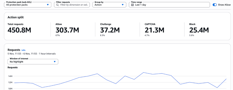
Figure 1: The security analytics dashboard across all protection packs
Dimensions
You can filter, group, and break down traffic by dimensions that include, but aren’t limited to, the following:
- Who’s sending traffic – Client IP, country, Autonomous System Number (ASN), user-agent, and JA4 TLS fingerprints
- What they’re requesting – Host, path (URI), protected resource (Amazon CloudFront distribution, AWS Application Load Balancers, and others), Region, or protection pack (web ACL)
- How AWS WAF responded – Action, rule triggered, labels, or response code
We’ll continue to add dimensions to the security analytics dashboard over time. The rest of this post refers to the preceding dimensions by the names used here. Two dimensions deserve a closer look:
- Host – Many customers think about their applications by domain rather than by protection pack (web ACL). Grouping or filtering by Host will show you which of your domains are under attack or if a spike is hitting www, the API, or a staging site, even when one protection pack (web ACL) protects several domains or one domain spans several protection packs (web ACLs).
- Labels – Labels are metadata that AWS WAF rules add to the requests they inspect. AWS Managed Rules for AWS WAF add them (for example, Bot Control labels for bot category, verification status, and signals such as
non_browser_user_agent), and you can create rules to add custom labels. Because labels are recorded even when a rule only counts, filtering by a label shows you what a rule detected across all of your protection packs (web ACLs), without changing how your traffic is handled.
Controls
The dashboard is built around a few controls:
- Filter requests – Combine conditions on any dimension, using Equals or Does not equal. Filters apply to the whole dashboard: the action split, the Requests chart, every widget, and the request list update to match. Your dashboard view is saved in your browser.
- Group by – Split the Requests chart by any dimension, such as Host, Rule triggered, Country, or JA4, to see how traffic changes over time.
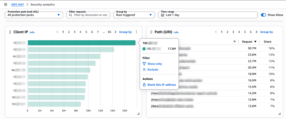
- Show only, Exclude, and Block – Select any value in any widget to focus on it, remove it from view, or block it. For example, you can block a high-risk or unexpected IP address, or block traffic from a country, directly from the dashboard.
- Requests and detections – Review the individual requests behind the charts. For each request, see HTTP request fields such as host, path, headers, user agent, and JA4 fingerprint. You can also see which detections and labels matched and whether each action was enforced or only counted . Previously, this level of detail meant working from a limited sample of requests or setting up and querying your own AWS WAF logs. Now it’s available directly on the dashboard.
Together, these controls help you answer questions such as:
- What share of traffic across all your protection packs (web ACLs) and domains is being blocked, challenged, or allowed, and how is it changing?
- Which rules are doing the most work, and are any of them blocking legitimate users?
- Which IP addresses, ASNs, JA4 fingerprints, or countries are behind a spike, and what are they targeting?
- How much of your traffic comes from bots, and are the bots verified?
Use case 1: Investigate a traffic spike
Suppose you receive an alert that blocked requests have increased. To investigate:
- Go to the Security analytics page in the AWS WAF console and select All protection packs.
- Assess the scope: The action split shows the overall block rate. Group the Requests chart by Host to see which domains are affected and check the Protection pack widget to see whether one application or several are involved. A campaign hitting your storefront, API, and media domains at the same time calls for a different response than a problem on a single endpoint.
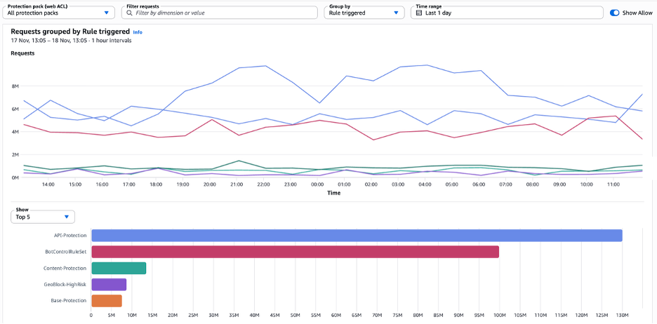
- Identify the source: Group the Requests chart by Rule triggered to see which rules are mitigating the traffic and when they started firing. Then check the source and request dimensions. If one IP address sends a disproportionate share of requests, or many IP addresses share one JA4 fingerprint, the traffic likely originates from a single automated actor.

Figure 2: Requests grouped by Rule triggered, showing which rules fired and when
- Confirm with request-level evidence: When you find an unexpected value, select it and choose Show only to filter the entire dashboard to it.
- Then confirm what you’re seeing in Requests and detections. Expanding a request shows all its details, including the HTTP request fields. For example, a curl user agent with no Accept-Language header, coming from a cloud hosting ASN, is likely automated traffic.
Figure 3: Show only, exclude, or block it
After you confirm the source, choose a response that fits the traffic:
- One clear source: Choose Block this IP address directly from the dashboard. Use a geographic block only if you don’t expect legitimate customers from that country.
- Traffic spread across multiple IP addresses: Add a rate-based rule with a custom aggregation key such as JA4, or use AWS WAF Bot Control.
- Known bad actors and application-layer floods: Add the Amazon IP reputation list and the Anti-DDoS managed rule group.
- Faster detection time: Create Amazon CloudWatch alarms on AWS WAF metrics. For details, see Monitoring with Amazon CloudWatch.
When the change is in place, return to the dashboard to confirm that requests from that source now show the Block action.
Use case 2: Tune your rules and reduce false positives
Rules can fail in two ways: by blocking legitimate users, or by only counting traffic that they should stop. Filters and labels help you find both.
If you suspect that a rule is blocking a broad population, such as many distinct clients sending only a few requests each, enter Rule triggered = <rule name> in Filter requests. The dashboard shows only the requests that the rule acted on. Review the Country, Host, and Path (URI) breakdowns to understand who the blocked clients are and what they requested. If the blocked clients look like your typical customers, with common browsers, expected countries, and checkout or login paths, consider adding a scope-down statement to the rule or changing the action to Challenge.
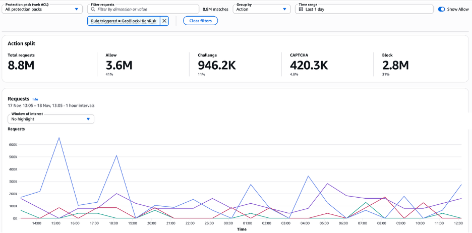
Figure 4: The dashboard filtered to a single rule with Filter requests
Evaluate rules before you enforce them: When you evaluate a managed rule group in Count mode, filter by its labels to see exactly which requests each rule matched. For example, filter by a Bot Control label such as awswaf:managed:aws:bot-control:bot:unverified, then check Host, Path (URI), and User-Agent to see what those bots are after. Use Exclude on labels for known-good traffic, such as bot:verified search engine crawlers, to keep them out of your review.
On the Detections tab of Requests and detections, rows marked Counted, not enforced show what a rule would block. If the matches aren’t partners or monitoring tools, consider changing the rule action to Block.
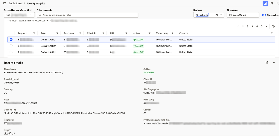
Figure 5: Record details for a single request, including host, JA4 fingerprint, and protection pack
After you change a rule, compare the same time window on the dashboard to confirm that the rule now affects only the traffic you intended.
Conclusion
The traffic overview dashboard shows you what changed in each protection pack (web ACL). The security analytics dashboard helps you understand why it changed, and lets you act on it from the same page, across all of your protection packs (web ACLs), domains, Regions, and Amazon CloudFront distributions. Filters, grouping, and labels explain the traffic, and request-level evidence helps you act with more confidence. Together, they can help you investigate faster, reduce how often real users are blocked by mistake, and confirm that each rule changes affect the traffic you intend.
The security analytics dashboard is available at no extra cost in all AWS Regions where AWS WAF is offered, and shows up to 21 days of request data. To get started, open the AWS WAF console and choose Security analytics.
If you have feedback about this post, submit comments in the Comments section below.
Related reading
To learn more about visibility and bot management in AWS WAF, see the following resources:
- Introducing the AWS WAF traffic overview dashboard
- Introducing AI traffic analysis dashboards for AWS WAF
- How to manage AI bots with AWS WAF and enhance security
- AWS WAF announces AI traffic monetization
If you have questions about this post, contact AWS Support or start a new thread on AWS re:Post.
CVE-2026-123890: Critical Authentication Bypass in VMware vCenter
Post Syndicated from Rapid7 original https://www.rapid7.com/blog/post/etr-cve-2026-123890-critical-authentication-bypass-vmware-vcenter
Overview
On November 19, 2026, Broadcom published VMware Security Advisory VMSA-2026-0009, addressing five vulnerabilities in VMware products. The most severe of these, CVE-2026-123890, is an authentication bypass using an alternate path or channel (CWE-288) in the VMware Directory Service component of vCenter. Broadcom assigned the vulnerability a critical CVSSv3 score of 9.8.
A malicious actor with network access to an affected vCenter deployment may exploit CVE-2026-123890 without credentials to bypass authentication and gain unauthorized access to the system as the Administrator user. Mandiant privately reported the issue to Broadcom. Also, Mandiant/Google Threat Intelligence confirmed in-the-wild exploitation of CVE-2026-123890 by Chinese state-linked threat actor ARMORY CASTLE as early as September 2026.
CVE-2026-123890 is distinct from the vCenter authentication bypass vulnerability CVE-2026-59309 that Broadcom addressed earlier in 2026. The vendor FAQ states that all vCenter systems below the versions fixed by VMSA-2026-0009 require the new update, including systems that already received the earlier fix. Broadcom characterizes the vCenter update as an emergency change requiring prompt action.
Mitigation guidance
Vendor-provided updates are available for CVE-2026-123890. Broadcom lists no workaround, and the patches cannot be applied using vCenter Quick Patch. Organizations should prioritize upgrading vCenter on an emergency basis, outside of normal patch cycles, using the standard update mechanism for their deployment.
|
VMware Product |
Affected Version |
Fixed Version / Patch |
|---|---|---|
|
VMware Cloud Foundation / vSphere Foundation |
9.1.x.x |
|
|
VMware Cloud Foundation / vSphere Foundation |
9.0.x.x |
|
|
VMware vCenter Server |
8.0 |
|
|
VMware vCenter Server |
7.0 |
Contact Broadcom Support (extended-support customers) |
|
VMware Cloud Foundation |
5.x |
|
|
VMware Telco Cloud Platform |
3.0, 4.x, 5.0.x, 5.1.x, 5.2 |
|
|
VMware Telco Cloud Infrastructure |
3.0 |
The fixes are cumulative. The vCenter 8.0 U3m and 9.0.2.0200 updates introduce a “Back-in-Time” restriction that blocks upgrades to VMware Cloud Foundation 9.1.1; Broadcom advises customers in an active upgrade to review the vendor FAQ and interoperability matrix. Updating vCenter temporarily makes its management interfaces unavailable, but Broadcom states that running virtual machine and container workloads continue to operate.
For the latest affected-version and mitigation guidance, please refer to Broadcom’s security advisory and supplemental FAQ.
Rapid7 customers
Exposure Command, Vulnerability Management, and Nexpose
Exposure Command, InsightVM, and Nexpose customers can assess exposure to CVE-2026-123890 on VMware vCenter Server with an unauthenticated vulnerability check expected to be available in the Nov 20, 2026 content release.
Updates
-
November 19, 2026: Initial publication.
Introducing Amazon EMR Serverless Flex: Run non-urgent Spark jobs at a discount
Post Syndicated from Neil Mukerje original https://aws.amazon.com/blogs/big-data/introducing-amazon-emr-serverless-flex-run-non-urgent-spark-jobs-at-a-discount/
With Amazon EMR Serverless, you can run Apache Spark applications without provisioning or managing clusters. You submit jobs, EMR Serverless allocates the compute, scales it during execution, and releases it when the job finishes. There are no clusters to tune and no idle capacity to pay for. Since launch, customers have used EMR Serverless to run production extract, transform, and load (ETL) pipelines, machine learning (ML) feature engineering, and large-scale data transformations, replacing Spark clusters that required dedicated engineering effort to operate.
Customers also have workloads that aren’t time-sensitive. On EMR on EC2 or self-managed Spark clusters on EC2, teams use Amazon Elastic Compute Cloud (Amazon EC2) Spot Instances to run these workloads on spare compute capacity at a lower cost. For top EMR customers, EC2 Spot Instances are a key cost-optimization lever, with many running a portion of their workloads on spare capacity. For customers looking to modernize from clusters to serverless to lower their operational overhead, the absence of an equivalent option on EMR Serverless meant they could only move part of their platform. The time-sensitive workloads came over, but the cost-optimized workloads running on spare capacity stayed on EC2 Spot Instances. Spare capacity support on EMR Serverless has been one of the most requested features, with customers telling us it’s a prerequisite for full migration.
Today we are launching Amazon EMR Serverless Flex, a new execution option that runs Spark batch jobs on spare compute capacity at a fixed 60 percent discount compared to standard pricing. With Flex, EMR Serverless now offers two execution options: Standard for workloads that need predictable start times and dedicated resources, and Flex for workloads where cost matters more than execution-time predictability. Customers who previously split their Spark platforms between EMR Serverless and EMR on EC2 or self-managed clusters on Spot Instances can now consolidate onto a single serverless platform. Customers who didn’t consider EMR Serverless at all, because spare capacity support was missing, can now evaluate EMR Serverless as a full replacement for their cluster-based deployments.
Why Flex matters for your Spark platform
When we talk to customers running Spark at scale, we see a common pattern: two tiers of workloads with different cost and reliability requirements.
Time-sensitive production workloads – ETL pipelines that feed dashboards, ML models, and downstream applications on a schedule. These need fast startup, dedicated compute, and predictable completion times. On EMR Serverless, these run on the Standard execution option.
Non-urgent batch workloads – Pre-production validation, test and development runs, backfills, nightly batch transformations, one-time data loads, and recurring reports with generous processing windows. These jobs are cost-sensitive but time-flexible. They need to finish, but not on a strict deadline.
On EMR on EC2 or self-managed Spark clusters on EC2, customers often deploy non-urgent workloads on Spot Instances. But without a spare-capacity option on EMR Serverless, moving to serverless meant giving up the cost lever on non-urgent batch workloads.
What it takes to run Spark on spare capacity today
On EMR on EC2, running Spark on Spot Instances is a shared responsibility between the service and the customer.
What the EMR service provides: EMR on EC2 provides the infrastructure features for running workloads on spare capacity:
- Instance fleets with Spot allocation strategies (capacity-optimized) that spread capacity requests across instance types and Availability Zones.
- Graceful decommissioning that gives Spark time to migrate shuffle data and finish running tasks when a Spot Instance receives a 2-minute termination notice.
- Spark resilience enhancements (decommission-aware task scheduling, exclusion of decommissioning nodes, and shuffle block tracking) that help Spark recover from node loss without getting stuck on fetch failures.
What customers implement: Based on best practices that have evolved over the years, here’s what teams have built and maintained on top of the preceding EMR features:
- Instance fleet diversification – Select the right mix of instance types across instance variants (
m5,m5a,m5d,r5,r5a,r5d) that meet vCPU and memory requirements. Use the Spot Instance Advisor to target types with lower interruption rates. Configure allocation strategies and fallback behavior. - Multi-AZ placement – Launch clusters targeting multiple Availability Zones to tap into the capacity in the entire AWS Region.
- Driver protection with YARN node labels – Configure YARN node labels to pin the Spark driver to On-Demand core nodes, keeping it off Spot task nodes. If the driver lands on a Spot Instance and that instance is reclaimed, the entire job fails. Setting this up requires YARN label configuration, node-label expression settings in Spark, and ongoing validation.
- Configuring resilience and decommissioning settings – Tune decommissioning timeouts, understand how the Spark resilience enhancements work, and configure them correctly for each workload.
- Ongoing tuning and debugging – Monitor interruption rates by instance type, adjust fleet composition as Spot pricing shifts, debug capacity-related job failures, and maintain the configuration as EMR release versions change.
What Flex handles for you
EMR Serverless Flex applies all of these spare-capacity best practices on your behalf. You add one parameter to your job submission with no fleet configuration or YARN tuning. EMR Serverless takes on the responsibility of running your workloads on spare capacity:
- AZ selection – EMR Serverless evaluates spare capacity pools across Availability Zones in the AWS Region and places workers where capacity is most available.
- Instance diversification – EMR Serverless spreads executors across multiple instance types and generations so that reclamation of one instance type doesn’t hit all workers at once.
- Driver protection – The Spark driver runs on a dedicated Standard worker that isn’t subject to spare capacity reclamation. The driver holds job state (the directed acyclic graph, stage progress, and task assignments) so protecting it prevents job failure, without YARN node labels to configure.
- Decommission-aware scheduling and worker exclusion – When a Flex worker receives a 2-minute reclamation notice, EMR Serverless stops scheduling new tasks on that worker and excludes it from future assignments. The Spark resilience enhancements that EMR developed for handling node loss (decommission-aware task scheduling, proactive worker exclusion, and shuffle block tracking) are applied automatically.
- Automatic task retry – Spark’s built-in fault tolerance retries affected tasks on healthy Flex workers. The job continues without manual intervention.
- Shuffle offload with Serverless Storage (optional) – With EMR Serverless Storage, shuffle data is written to remote storage instead of local disk. When a reclaimed executor’s tasks are retried, the new executor reads the stored upstream shuffle output instead of recomputing it, reducing the fetch-failure problem for shuffle-heavy jobs.
All existing EMR Serverless capabilities (AWS Lake Formation fine-grained access control, AWS Graviton support, AWS Glue Data Catalog integration, and data source connectors) work the same with Flex jobs.
What happens when you run a Flex job
Here is the life cycle of a Flex job from submission to completion:
- Job submission – You submit a Spark job with Flex enabled. EMR Serverless accepts the job and begins acquiring spare compute capacity.
- Capacity acquisition – EMR Serverless selects an Availability Zone within the chosen Region where spare capacity is most available and requests workers across a diverse set of instance types and generations. The Spark driver starts on a dedicated Standard worker.
- Job execution – Executors run on Flex workers. The job proceeds as it would on Standard using the same Spark runtime and APIs.
- If capacity is reclaimed – When a Flex worker receives a reclamation notice, EMR Serverless excludes it and stops scheduling new tasks on it. Spark retries the affected tasks on healthy Flex workers. If you have Serverless Storage enabled, retried tasks read stored shuffle data instead of recomputing upstream stages. Billing for the reclaimed worker stops at reclamation.
- Completion – The job completes and results are written to the output location.
- Failure handling – If no executor joins the driver within 20 minutes of job start, the job fails. To recover from failures, resubmit the job using the best practices you apply to restart a failed job.
How Flex workers are billed
Flex workers are billed at a fixed 60 percent discount on vCPU-hours and memory GB-hours compared to Standard workers. The Spark driver runs on a Standard worker and is billed at the Standard rate. The discount is fixed and unlike EC2 Spot doesn’t fluctuate with supply and demand.
Each worker is billed for the time it was part of the job run, per second with a 1-minute minimum. When a Flex worker is reclaimed, billing for that worker stops. For example, if a 10-minute job runs 20 Flex workers and 3 of them are reclaimed after 5 minutes, you are billed for 17 workers at 10 minutes and 3 workers at 5 minutes.
Flex spend appears as separate line items in AWS Cost Explorer and on your bill, so you can distinguish Flex spend from Standard spend. Flex also works with job-level cost allocation tags, so you can continue attributing costs by team or project. For pricing details, see Amazon EMR pricing.
Flex in practice: Resilience and cost
We ran a 103-query decision-support benchmark (derived from TPC-DS 1 TB and 3 TB scale factor) on Spark to compare Flex and Standard at two data scales. Both runs used the same queries, worker configuration, and release label (emr-7.14.0).
| Scale factor | Execution | Queries completed | Wall-clock time | Estimated cost | Total executors used | Executors reclaimed | Task failures |
| 1 TB | Standard | 103 of 103 | 11.5 min | $5.68 | 12 | 0 | 0 |
| Flex | 103 of 103 | 12.3 min | $2.07 (64% savings) | 15 | 1 | 0 | |
| 3 TB | Standard | 103 of 103 | 12.4 min | $6.29 | 12 | 0 | 0 |
| Flex | 103 of 103 | 16.1 min | $2.32 (63% savings) | 21 | 1 | 0 |
Resilience: In each Flex run, we observed one executor reclaimed mid-job. EMR Serverless excluded the reclaimed worker, and Spark retried the affected tasks on healthy executors. All 103 queries completed in both runs, with zero job resubmissions.
Cost: For this benchmark, we saw Flex reduce estimated cost by about 63 percent at both data scales, from $5.68 to $2.07 at 1 TB, and from $6.29 to $2.32 at 3 TB.
Note: The actual savings and frequency of reclamations will vary by workload, Region, and available spare capacity at the time of execution. We recommend running your own workloads on both Flex and Standard to establish a baseline. This workload is derived from the TPC-DS Benchmark and isn’t comparable to published TPC-DS Benchmark results, as this implementation doesn’t comply with all requirements of the TPC-DS Benchmark.
Runtime tradeoff – The 1 TB Flex run took 7 percent longer than Standard. The 3 TB run took 30 percent longer. The gap widened at larger scale because the reclaimed executor’s tasks needed more time to recompute. Flex jobs can also take longer to start if spare capacity isn’t immediately available. Flex works well for any job where the completion deadline is flexible, including short jobs. A job that runs in 10 minutes on Standard and 12 minutes on Flex is a good candidate if it doesn’t have a strict service level agreement (SLA).
Getting the best results from Flex
Three practices we recommend to get the most from Flex:
Avoid top-of-the-hour peaks
We observe that spare capacity availability drops when many jobs start simultaneously at the top of each hour. Shifting your job start times by even a few minutes (for example, submitting at 9:20 instead of 9:00) reduces contention for spare capacity and improves the chance of a fast start.
Run outside business hours when possible
Spare capacity is most available when overall compute demand is lower. We see the best availability when customers schedule non-urgent workloads to run after 6:00 PM in the Region, or on weekends, giving Flex jobs access to deeper capacity pools with fewer interruptions.
Use Serverless Storage
EMR Serverless Storage writes shuffle data to remote storage, so retried tasks read stored intermediate results instead of recomputing upstream stages. This reduces the runtime cost of interruptions on shuffle-heavy jobs and adds another layer of resilience.
Getting started
Flex is a job-run setting. You create your EMR Serverless application as usual and add one parameter when submitting a job:
In EMR Studio, select the Enable Flex execution checkbox when submitting a job, as shown in the following screenshot:
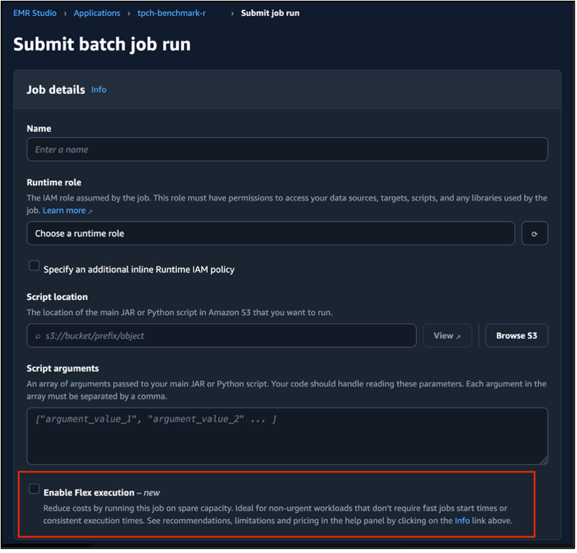
Figure 1: Enable Flex execution checkbox in the EMR Studio job submission form
You can run Flex and Standard jobs on the same application. For step-by-step instructions, see the Amazon EMR Serverless User Guide.
Conclusion
In this post, we shared how Amazon EMR Serverless Flex runs non-urgent Spark batch jobs on spare compute capacity with built-in resilience features, closing a gap that previously blocked customers from modernizing their entire Spark platforms onto EMR Serverless.
To get started, pick a non-critical job, submit it with --flex-execution '{"enabled": true}' and compare the cost and runtime against your Standard baseline. For more detail, see the Amazon EMR Serverless User Guide.
About the authors
Announcing 30-minute timeout for on-demand AWS Lambda Event Functions
Post Syndicated from Tarun Rai Madan original https://aws.amazon.com/blogs/compute/announcing-30-minute-timeout-for-on-demand-aws-lambda-event-functions/
AWS Lambda now supports a 30-minute function timeout for Event Functions that run on demand, doubling the previous 15-minute limit for synchronous, asynchronous, and event source mapping (ESM) invocations. On Lambda Managed Instances, synchronous invocations also support up to 30 minutes, while asynchronous and ESM invocations keep the 90-minute timeout we announced in September 2026. You can now run AI inference, media transcoding, and financial calculations on Lambda for spiky or steady-state traffic without re-architecting your applications. The new timeout also applies when you use Lambda durable functions or invoke your functions from AWS Step Functions Standard workflows.
Evolution of function timeout on Lambda
Lambda launched in 2014 with a 60-second function timeout, which we extended to 5 minutes in 2015 and to 15 minutes in 2018.
Lambda now offers three form factors: Event Functions, Web Functions, and MicroVMs. Event Functions process events from more than 200 AWS event sources through synchronous, asynchronous, and ESM invocations. With Web Functions, you can run HTTP servers on Lambda with an HTTP-native, multi-concurrent programming model and opt-in multi-Region endpoints. MicroVMs give each user or session an isolated environment for running user-generated or AI-generated code.
By default, all three form factors run on demand, with Lambda provisioning compute as requests arrive. For steady-state traffic, Event Functions can also run on the Lambda Managed Instances capacity provider. With Lambda Managed Instances, you can process multiple concurrent requests per instance and choose specialized compute configurations, without managing infrastructure. You can also use EC2 pricing options such as AWS Savings Plans and Reserved Instances. Figure 1 shows the form factors.
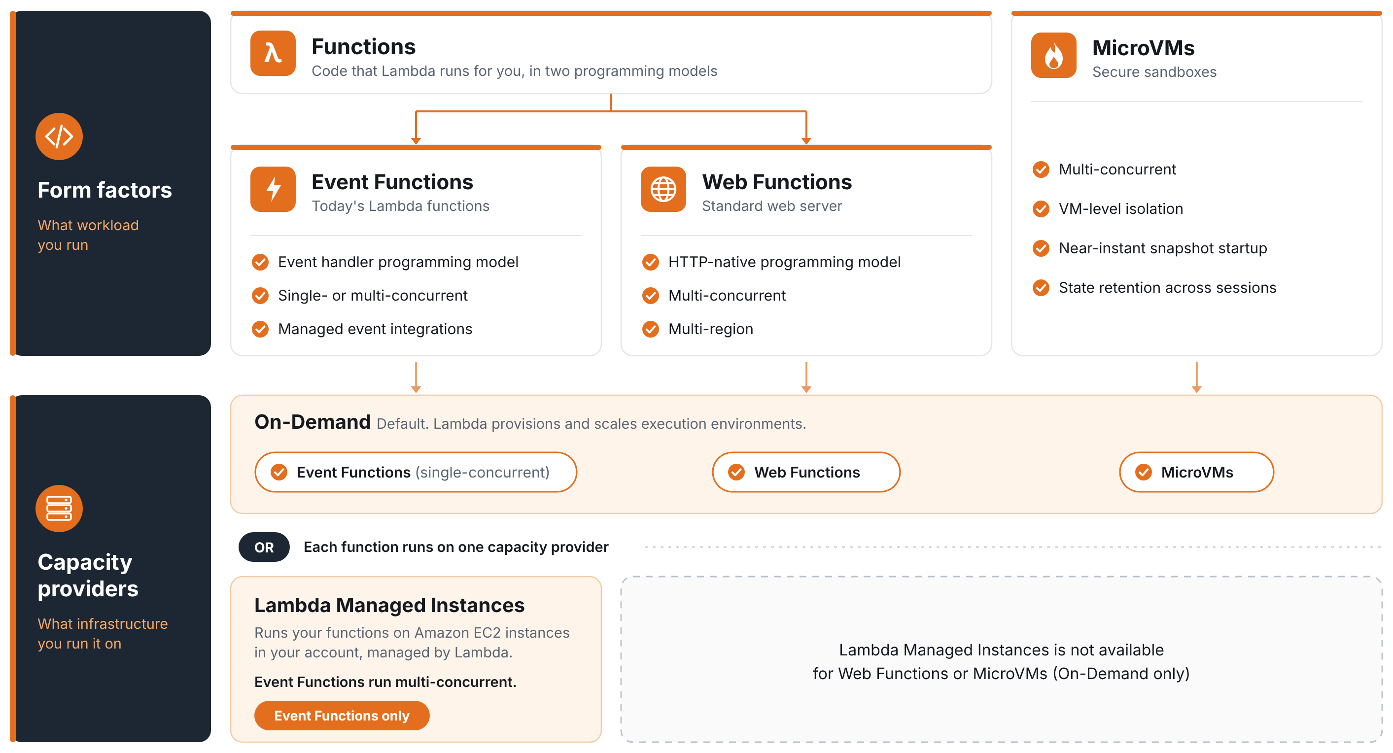
Figure 1: Lambda form factors
Each form factor has its own duration limit (Table 1). Until today, Event Functions had a 15-minute timeout, except for asynchronous and ESM invocations on Lambda Managed Instances, which we extended to 90 minutes in September 2026.
Lambda durable functions run on demand and on Lambda Managed Instances, and provide application-level checkpointing and workflow-as-code. Your code saves execution state with step() and wait() operations and resumes from the last checkpoint after a failure. A durable execution (the complete lifecycle of a durable function) can run for up to 1 year, but each invocation within it is bound by the function timeout.
Customers told us that 15 minutes was still too short for many Event Functions workloads that run on demand, and for synchronous invocations on Lambda Managed Instances. Agentic AI requests that chain model calls and tool invocations can take longer than 15 minutes to return a result. Media transcoding and file conversion jobs often run past 15 minutes when input files are large. Financial calculations such as Monte Carlo simulations, bond pricing, and portfolio risk analysis are memory-intensive and need more continuous execution time. Report generation across multiple data sources can also exceed 15 minutes during peak volumes. ETL steps triggered by Amazon Simple Queue Service (Amazon SQS) or Amazon Simple Storage Service (Amazon S3) events can run just as long. Many of these workloads have spiky traffic that doesn’t justify steady-state capacity on Lambda Managed Instances.
With today’s launch, Event Functions support up to 30 minutes for synchronous, asynchronous, and ESM invocations, and up to 90 minutes for asynchronous and ESM invocations on Lambda Managed Instances. Table 1 shows the maximum durations across Lambda form factors.
| Duration | Event Functions | Web Functions | MicroVMs | |
| On demand (default) | Lambda Managed Instances | |||
| Without durable execution |
Synchronous: 30 minutes Asynchronous: 30 minutes ESM: 30 minutes |
Synchronous: 30 minutes Asynchronous: 90 minutes ESM: 90 minutes |
15 minutes | 8 hours (running and suspended) |
| With durable execution |
Synchronous: 30 minutes Asynchronous: 1 year ESM: 30 minutes |
Synchronous: 30 minutes Asynchronous: 1 year ESM: 90 minutes |
– | – |
Table 1: Supported durations on Lambda form factors
Configuring the 30-minute function timeout
You can configure any Event Function with a timeout of up to 30 minutes (1,800 seconds). For asynchronous and ESM invocations on Lambda Managed Instances, you can configure up to 90 minutes (5,400 seconds). Lambda rejects higher values with a validation error. Your function runs exactly as before, with the same runtime, handler, IAM execution role, and virtual private cloud (VPC) configuration. The Init phase keeps its existing limits of 10 seconds for functions that run on demand and 15 minutes on Lambda Managed Instances. Provisioned concurrency and Lambda SnapStart, which aren’t available on Lambda Managed Instances, keep their 15-minute initialization limit.
To set the timeout, update your function configuration using the AWS Command Line Interface (AWS CLI):
To set the timeout in an AWS Serverless Application Model (AWS SAM) template, use the Timeout property:
You can also update the timeout in the Lambda console under Configuration > General configuration (Figure 2), where synchronous test invocations now run for up to 30 minutes. If you use an AI coding assistant such as Kiro, Claude Code, or Codex, you can install the Agent Toolkit for AWS and configure the timeout with natural language prompts.
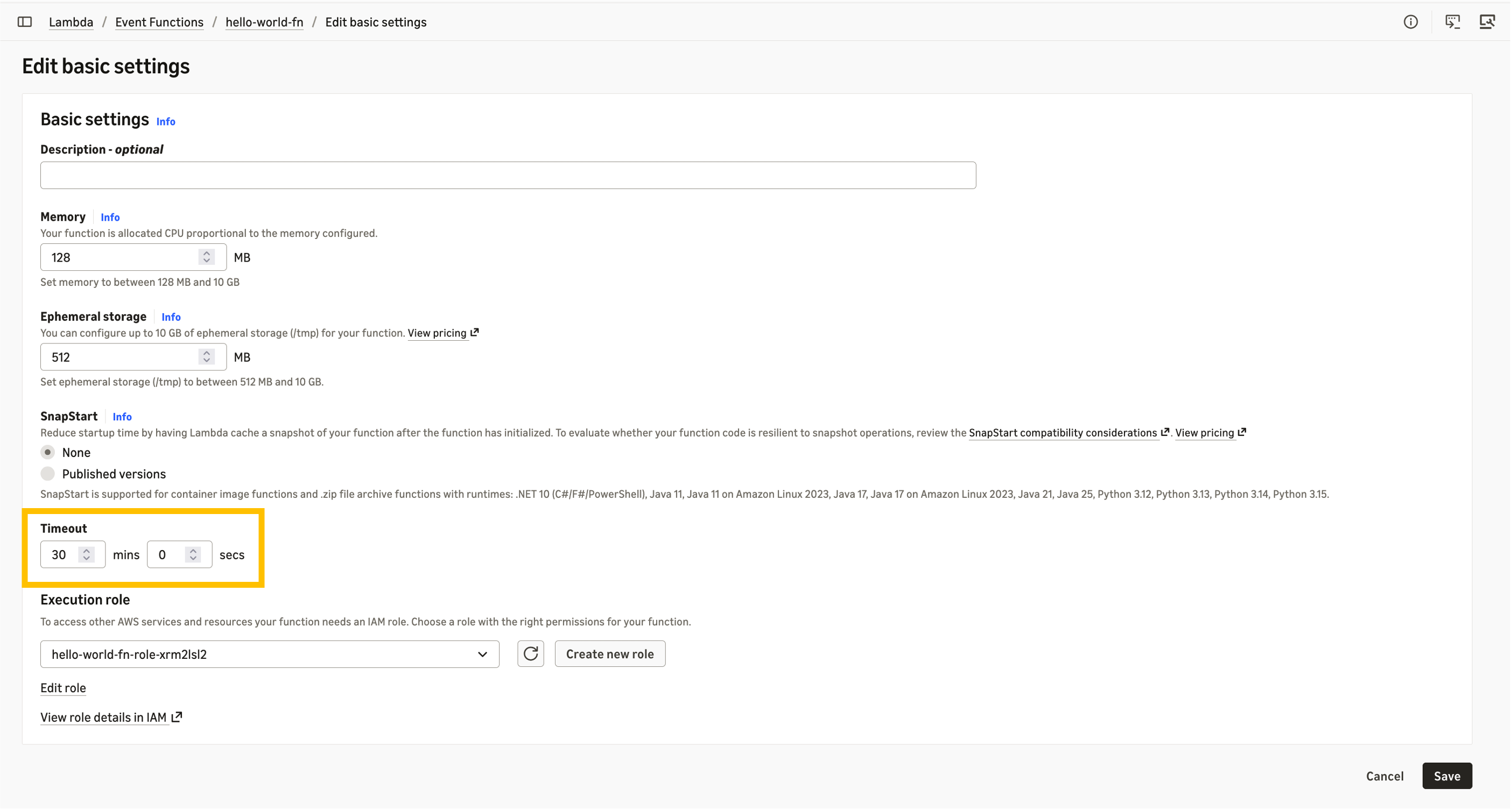
Figure 2: Configuring Lambda function timeout
The new timeout applies to invocations that start after you update the function. For event source mappings, allow a few minutes for the change to propagate. Amazon CloudWatch metrics, AWS CloudTrail, and AWS X-Ray continue to capture the full invocation lifecycle. For details, see monitoring Lambda functions and monitoring durable functions.
For Event Functions that run on demand, the 30-minute timeout is available in all commercial AWS Regions. For synchronous invocations on Lambda Managed Instances, it is available in all AWS Regions where Lambda Managed Instances is available. Standard AWS Lambda pricing applies.
30-minute timeout and durable functions
The 30-minute function timeout and durable functions are complementary. The function timeout (--timeout) controls how long each individual invocation can run, whereas the durable execution timeout (ExecutionTimeout in --durable-config) controls the total elapsed time from execution start to completion. On replay after a failure, the function re-executes from the beginning and skips completed steps.
Functions that run on demand: Each durable function invocation can run for up to 30 minutes, whether you invoke it synchronously, asynchronously, or through an event source mapping. When you invoke the function asynchronously, the durable execution can run for up to 1 year. When you invoke it synchronously through the Invoke API or a function URL, the durable execution is limited to 30 minutes, and Lambda rejects higher values. ESM invocations have the same 30-minute limit.
Lambda Managed Instances: Synchronous invocations can run for up to 30 minutes, and asynchronous and ESM invocations can run for up to 90 minutes. When you invoke the function asynchronously, the durable execution can run for up to 1 year. The durable execution is limited to 30 minutes for synchronous invocations and 90 minutes for ESM invocations.
For idempotent jobs, such as an ETL step triggered by Amazon SQS, the extended timeout alone might be enough. A failed invocation returns the message to the queue for a fresh attempt. For jobs where re-execution is expensive, combine the extended timeout with durable functions. A 25-minute inference run that fails at minute 22 restarts from zero without checkpoints, but resumes from its last checkpoint with durable functions.
Invocation behavior: Synchronous, asynchronous, and event source mappings
Synchronous invocations (up to 30 minutes): Synchronous invocations now support up to 30 minutes, whether the function runs on demand or on Lambda Managed Instances. If another AWS service invokes your function synchronously, that service applies its own timeout, so verify that it supports the longer duration before you raise the function timeout. Set your client’s read and socket timeouts longer than the function timeout. For example, increase the read timeout of your AWS SDK client when you call the Invoke API. On Lambda Managed Instances, Lambda applies the 30-minute limit to synchronous invocations even if the function timeout is higher, and the GetFunctionConfiguration API reports the configured value.
Asynchronous invocations (up to 30 minutes, or up to 90 minutes on Lambda Managed Instances): If the function fails or times out, Lambda applies your configured retry policy (up to two retries by default). It then routes failed events to your dead-letter queue or on-failure destination.
Event source mappings (up to 30 minutes, or up to 90 minutes on Lambda Managed Instances): For SQS, set the queue’s visibility timeout to at least six times the function timeout, so at least 3 hours for a 30-minute function. This gives Lambda enough time to retry if a function is throttled while it processes a previous batch. Lambda validates this when you create the event source mapping, but it doesn’t prevent later changes to queue or function settings that create a mismatch.
For Amazon Kinesis Data Streams and Amazon DynamoDB Streams, Lambda processes one batch per shard at a time by default, so longer invocations slow how quickly each shard is read. Monitor the IteratorAge metric and increase the parallelization factor if records start to back up. Longer invocations also mean that a failure late in a batch wastes more work. Enable partial batch failure reporting so that Lambda retries only the failed records. You can use it with SQS, Amazon Kinesis, DynamoDB Streams, Amazon Managed Streaming for Apache Kafka (Amazon MSK), and self-managed Apache Kafka event source mappings.
Invocations from Amazon MQ (ActiveMQ and RabbitMQ) and Amazon DocumentDB (with MongoDB compatibility) event source mappings remain limited to 14 minutes. The same limit applies to Kafka event source mappings that were created before November 19, 2026, and don’t use provisioned mode. To use the 30-minute timeout with Kafka, create a new event source mapping or turn on provisioned mode for your existing one. For these mappings, keep the function timeout at 14 minutes (840 seconds) or less.
Considerations and best practices
Longer-running functions need extra care with concurrency and components that can expire mid-invocation, such as network connections and credentials.
Concurrency: Concurrency equals requests per second multiplied by average duration in seconds. At the same request rate, a function that runs for 30 minutes instead of 15 needs twice the concurrency. For example, 1 request per second at 30 minutes each needs 1,800 concurrent executions. Check your account concurrency quota and reserved concurrency settings before you raise the timeout. On Lambda Managed Instances, check the maximum scaling limits of your capacity provider.
Networking: Make sure idle connection timeouts on downstream services such as Amazon Relational Database Service (Amazon RDS), Amazon ElastiCache, and external APIs accommodate the full function duration. If your function routes traffic through a NAT gateway, which drops idle connections after 350 seconds, send keep-alive packets. For long synchronous invocations, also turn on TCP keep-alive on the calling client. DNS caching depends on your runtime and HTTP client. For example, the AWS SDK for Java relies on the JVM DNS cache, which on some configurations never refreshes. Set a short DNS TTL, such as 5 seconds for the JVM, and configure custom HTTP clients to re-resolve hostnames.
Credentials: If your function acquires temporary credentials or tokens, verify they remain valid for the full execution duration or refresh them in the background.
Idempotency: Lambda does not guarantee exactly-once processing, and longer-running functions widen the window for retries and duplicate deliveries. Use Powertools for AWS Lambda to make operations such as payments or database writes idempotent. In durable functions, steps have at-least-once execution semantics by default. The SDK skips completed steps during replay, but steps that fail before checkpointing might re-execute. You can use execution names as idempotency keys for durable functions.
Conclusion
The 30-minute function timeout brings longer continuous execution to Event Functions that run on demand and to synchronous invocations on Lambda Managed Instances. It complements the 90-minute timeout for asynchronous and ESM invocations on Lambda Managed Instances that we launched in September 2026. Workloads such as AI inference, media transcoding, and report generation that exceed 15 minutes can now run on Lambda without architectural workarounds, for spiky or steady-state traffic. If your workloads need a longer timeout, let us know on the AWS Lambda Roadmap GitHub page.
To get started, update your function’s timeout configuration and deploy. For details, see Configure Lambda function timeout in the AWS Lambda Developer Guide. For sample code that shows long-running functions with durable checkpointing, see durable functions examples. To learn more, visit the AWS Lambda product page.
About the authors
How AWS Security Incident Response triages your security findings
Post Syndicated from Anatoliy Kochetov original https://aws.amazon.com/blogs/security/how-aws-security-incident-response-triages-your-security-findings/
AWS Security Incident Response continuously triages the threat findings from Amazon GuardDuty and AWS Security Hub CSPM, but most of that work never shows up as a case. If cases are all you look at, it’s hard to tell whether the service is working at all, and that’s the question I hear most often when I help customers onboard. The Proactive response dashboard gives you a high-level view of this activity, and this post takes you behind the numbers to show what happens to an individual finding.
In this post, I walk you through what happens to a finding after it’s ingested by the service, what gets triaged, where each finding is sent, and how a triage decision becomes a case. I then show you how to confirm triage is working day-to-day, so your team can focus on the findings that require attention. The process flow is shown in Figure 1.
Figure 1: AWS Security Incident Response triage flow, from ingestion through to one of three outcomes
Ingestion
AWS Security Incident Response ingests threat findings from GuardDuty through Amazon EventBridge rules that are automatically deployed to your accounts during the onboarding process.
If you send third-party detection findings to Security Hub CSPM from tools such as CrowdStrike, Trend Micro, or Lacework, their threat detection findings are also ingested. Each of those findings must carry complete payload information such as resource ID, account ID, timestamp, and threat details. GuardDuty findings are ingested directly, so these findings aren’t re-ingested through Security Hub CSPM and there’s no duplication.
Triage
The service triages findings that indicate an active threat, such as compromised credentials, cryptomining, or data exfiltration. These represent activity that’s underway or has already occurred.
Posture and compliance findings aren’t triaged. A misconfiguration or a failed benchmark check reflects the state of your environment rather than an active threat, so those findings remain for your team to address through your existing remediation process.
Outcomes
For each threat finding, the service runs an automated triage process. It evaluates the finding payload, related AWS activity from AWS CloudTrail and Amazon VPC Flow Logs, AWS threat intelligence, and the context you provide about your environment. The service then maps the finding against a profile of known-good activity. What fits the profile is treated as expected, and what doesn’t is flagged for a closer look.
What happens next depends on that outcome. A finding is sent to one of three places:
- Archived, no action needed – Automated triage or an AWS Security Incident Response engineer confirms the activity is benign or expected. The finding is archived in GuardDuty, with no case and no customer contact.
- A proactive case is opened – Triage can’t confirm the activity is benign. This is either Unconfirmed Activity (the service needs you to confirm whether it’s expected) or Inappropriate/Unintended Activity (confirmed activity that needs your action). A proactive case is opened, your incident response team is engaged, and the finding stays Current until it’s resolved.
- Retained for your review, no case – Posture-related findings, such as overly permissive policies, configuration, or missing encryption, aren’t threats. By design, they stay Current without archiving and no case is created.
When a proactive case is opened, you respond to it in the AWS Management Console for AWS Security Incident Response under Cases, where you can communicate directly with the team, share context, and resolve or reopen the case. Timely responses also help the service learn your environment, which helps reduce false positives over time. For the full workflow, see Responding to an AWS generated case.
The preceding outcomes use GuardDuty terms, because it’s the primary source. Third-party findings ingested through Security Hub CSPM follow the same triage logic, but their disposition shows as a workflow-status change rather than archiving. The finding moves from NEW to NOTIFIED when triage begins, which removes it from the default Security Hub CSPM view. If triage clears it as benign, it moves to SUPPRESSED. Otherwise it stays visible for your review.
Because only benign findings are archived, it’s normal to see many findings in Current, and that isn’t a sign the service missed them. Across customers, less than 1 percent of ingested findings result in a customer-facing escalation. Most are handled automatically, without a case.
Credential exfiltration finding example
Suppose GuardDuty generates an UnauthorizedAccess:IAMUser/InstanceCredentialExfiltration.OutsideAWS finding: temporary credentials created on an Amazon Elastic Compute Cloud (Amazon EC2) instance were used from an IP address outside AWS. Triage cross-references the payload against what it knows about your environment.
- Cleared – The external IP belongs to a corporate virtual private network (VPN) range that your workloads regularly call through, and the service has seen this pattern before. The finding is archived in GuardDuty.
- Escalated – The IP is in a hosting-provider range with no prior association to your accounts, and the AWS Identity and Access Management (IAM) role has never made calls from outside AWS. The service creates a proactive case, notifies your incident response team, and an engineer investigates whether the credentials were compromised.
Same finding type, two outcomes. The difference is context, and context is what triage builds by observing your environment over time.
How triage sharpens over time
The service builds a profile of what’s normal in your environment. It learns the IP ranges and domains you trust, and the IAM principals and behaviors your workloads rely on. When your team routinely connects from a known VPN range, or a specific IAM role runs nightly batch jobs, the service recognizes those patterns and measures new findings against them. Early on, engineers investigate more findings by hand as they learn your environment. Within a few weeks, automated triage handles most of those decisions on its own.
Triage is dynamic. A finding treated as expected today can be re-evaluated tomorrow if the context changes, so the service can still catch a real threat that reuses a pattern it formerly treated as safe. You can shape the profile by submitting known-good activity, such as trusted IP ranges or authorized scanning tools, through an AWS Support case. For details, see Submit known-good activity.
Archiving versus suppression
It’s possible to conflate the two mechanisms, so it’s worth separating them:
- Archiving is the primary mechanism. When automated triage or an engineer determines a finding is benign, the service archives it in GuardDuty. The finding then stays there for 90 days.
- Suppression rules are less common and work differently. A suppression rule acts on future findings. When the service identifies a recurring pattern of expected activity, it might create a GuardDuty suppression rule that automatically archives matching findings so they don’t generate new alerts. Suppressed findings aren’t sent to your configured export, such as an Amazon Simple Storage Service (Amazon S3) bucket or SIEM. When the service creates a rule, your incident response team is notified, and you can view and manage it in the GuardDuty console under Suppression rules.
A healthy deployment typically shows many archived findings and few or no suppression rules. That’s expected, and it means the service is handling findings dynamically rather than relying on static filters.
How to see what triage is doing
Triage runs on its own, and the service gives you a few ways to confirm it’s working.
Proactive response dashboard
The Dashboard page in the AWS Security Incident Response console has a Proactive response section. It counts how many findings were ingested, triaged, investigated, and escalated over the timeframe you select, the last 7, 30, or 90 days.
The Overview leads with two figures. Noise reduction is the share of ingested findings that automated triage resolved without opening a case, so you can see for yourself how much volume never reached your team. Time saved estimates the analyst hours that automation returned to you, counted as one hour for each ingested finding.
Below that, Finding evaluations breaks those stages down:
- Ingest – Threat findings collected from your detection sources
- Triage – Findings evaluated automatically to decide whether the activity is expected
- Investigation – Findings automated triage couldn’t confirm, passed to an AWS Security Incident Response engineer for a closer look
- Escalation – Investigations raised as a case when a genuine risk was detected or the activity couldn’t be confirmed as expected
A flow diagram on the dashboard shows how those findings move from their sources through triage and investigation, with branches for the ones closed as false positives and the ones still in progress. For more, see Viewing proactive response metrics.
Monthly report
The monthly report is the periodic companion to the dashboard. AWS Security Incident Response emails it to your incident response team a week or two after each month closes. It opens with the accounts monitored, findings processed, and investigations, then lists each investigation and its status, the triage flows that show the checks run for each finding type, and the context the service has learned about your environment, such as the trusted networks it now recognizes as normal.
Archived findings in GuardDuty
For a quick confirmation outside either view, open Findings in the GuardDuty console and filter to see Archived. That list also includes findings archived by you or by suppression rules, so look for the threat findings AWS Security Incident Response archived after triage. Each one is a finding that the service cleared as benign so your team didn’t have to.
Conclusion
AWS Security Incident Response continuously evaluates your threat findings so your team can spend its time on confirmed threats rather than alert volume. Findings that are evaluated as benign are archived automatically, the ones that need a response become proactive cases, and posture issues stay in Current for your team to handle.
Cases show only a small part of that work. When I deliver AWS Security Incident Response to customers now, I walk them through the triage flow in Figure 1, the Proactive response dashboard, and their monthly report, so they can see how triage works end to end.
To get started, see the onboarding guide. Setup takes about 10 minutes. For more information, see the AWS Security Incident Response product page or the User Guide.
If you have questions about this post, contact AWS Support or start a new thread on AWS re:Post.
AWS Lambda Durable Functions observability with OpenTelemetry
Post Syndicated from Ricardo Marques original https://aws.amazon.com/blogs/compute/aws-lambda-durable-functions-observability-with-opentelemetry/
Gaining observability into AWS Lambda Durable Functions, a capability of AWS Lambda, can be challenging. A single workflow can span multiple invocations, queues, and downstream services, with no persistent host or centralized log file to inspect. With OpenTelemetry, you can close that gap by generating and correlating traces, metrics, and logs through an open specification. You can instrument once and export anywhere, which avoids vendor lock-in and establishes a baseline for operating serverless systems at scale.
With AWS Lambda Durable Functions, you can construct resilient workflows with multiple steps, which save their state and automatically recover from errors by replaying. A single durable execution can persist across several Lambda calls. It can continue after pauses, recover from errors, and restart from saved checkpoints. Although this model delivers fault tolerance, it introduces an observability challenge. Each invocation generates its own trace, fragmenting the end-to-end view of a single logical workflow.
This post introduces the OpenTelemetry plugin for the AWS Durable Execution SDK (aws-durable-execution-sdk-python-otel). With this plugin, you can generate deterministic trace IDs that unify all invocations of a single durable execution into one coherent distributed trace. In this post, you learn how to set up the plugin, see the traces it produces for the happy-path workflow, and apply foundational best practices.
The complete application code is available in our GitHub repository, so this post uses code snippets to illustrate the examples.
The problem: fragmented traces across invocations
Consider a document review workflow with a human approval gate:
This workflow runs across at least two Lambda invocations. The first invocation executes extract-text and summarize, then suspends at human-review with zero compute cost while waiting. Hours later, when the reviewer responds, Lambda invokes the function again. It replays the completed steps and executes publish.
The following diagram illustrates the difference between the default behavior and the plugin’s unified tracing. On the left side, two independent traces are generated: Trace A captures the first invocation (totaling 2.69 seconds), while Trace B captures the second invocation after the callback resumes (replaying and publishing in 0.37 seconds). These traces have different trace IDs and no correlation between them. On the right side, with the OTel plugin, all operations appear under a single deterministic trace ID. The human-review wait (6 hours and 8 minutes at zero compute cost) is represented as a continuous span connecting both invocations, giving operators a complete timeline from start to finish. You can compare the total wall-clock duration of 152 seconds against only 0.019 seconds of actual compute time billed.
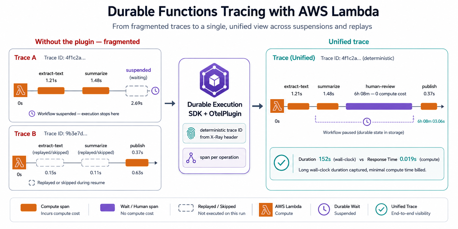
Figure 1. Trace comparison of fragmented traces without the plugin (left) versus a single unified trace with the OTel plugin (right), showing how the Durable Execution SDK merges multiple Lambda invocations into one end-to-end trace.
The plugin achieves this through:
| Capability | What it does |
| Deterministic trace IDs | Derives a stable trace ID from the AWS X-Ray header, so all invocations share one trace |
| Span-per-operation | Each step, wait, or wait_for_callback gets its own span with real timing |
| Continuation spans | Operations completing in a later invocation link back to the original span |
| Log correlation | Stamps traceId and spanId onto every log record automatically |
| Configurable sampling | Standard OpenTelemetry sampling to control trace volume |

Figure 2. Amazon CloudWatch Application Signals Traces view. The durable execution appears as a single trace with OK status. The Duration column (152s) reflects the total wall-clock time including the human-review wait, while Response Time (0.019s) shows only the compute time.
Choose execution view to see all operations grouped under the Workflow span. Use this view when the full execution, including waits and retries, finishes within your tracing vendor’s span ingestion window. For example, if your vendor rejects spans that started more than 8 hours ago, use execution view only for workflows that reliably finish well under 8 hours.Choose invocation view if an execution might exceed your vendor’s ingestion window, or if you want to see progress as each function execution terminates. Operations appear under the invocation that ran them. A wait’s first segment appears under the invocation that started it, even while the wait is still pending.In both views, the Workflow span covers the full execution, so the vendor’s ingestion window still applies to it. If an execution runs longer than the window, your vendor might reject the Workflow span even in invocation view.
The plugin sends Workflow as one span when the execution succeeds or fail. It doesn’t send that span in pieces. The vendor can, however, accept earlier spans from the same trace.
Why do we recommend someone to use invocation view for long running ones?Suppose a workflow waits 10 hours and the vendor rejects spans that started more than 8 hours ago. In invocation view, the invocation that starts the wait can export the wait’s initial span before the wait finishes. The invocation that resumes the workflow can later export the wait’s completion span. Those short spans can be accepted even if the vendor rejects the final Workflow span.
Getting started
In the following walkthrough, you configure your Lambda durable function to trace requests end-to-end.
Prerequisites
- Python 3.11 or later.
- An existing Lambda durable function (or a new one you want to instrument).
- An AWS account with permissions to enable Amazon CloudWatch Application Signals tracing and add Lambda layers.
Step 1: Install the plugin
Add the plugin to your function’s dependencies:
Or in your requirements.txt:
Step 2: Add the ADOT Lambda layer
With the AWS Distro for OpenTelemetry (ADOT) Lambda layer, you can export traces from your function.
Note: The examples in this post use AWS Serverless Application Model (AWS SAM) for brevity. You can achieve the same configuration using the AWS Command Line Interface (AWS CLI), AWS Cloud Development Kit (AWS CDK), Terraform, or AWS CloudFormation directly. Refer to the ADOT Lambda Layer ARNs page for the latest layer version and supported architectures. Pin the layer version in production deployments to avoid unexpected behavior from automatic version changes.
Step 3: Turn on X-Ray active tracing
The plugin uses the _X_AMZN_TRACE_ID environment variable to derive deterministic trace IDs. Turn on active tracing on your function:
Also verify your function’s execution role includes the AWSXRayDaemonWriteAccess managed policy (or equivalent xray:PutTraceSegments and xray:PutTelemetryRecords permissions).
Step 4: Add the OTel plugin to your handler
Import InvocationOtelPlugin and pass it to the plugins parameter of @durable_execution:
The plugin handles Tracer Provider setup, deterministic ID generation, and span lifecycle internally.
Testing and results
After you configure the plugin, deploy the function, invoke it, and confirm the unified trace appears in Amazon CloudWatch.
Testing the setup
Build and deploy your function:
Then publish a function version (durable functions require a qualified ARN, not $LATEST):
Invoke the function asynchronously (required when using wait_for_callback, since the function suspends mid-execution):
Monitor the logs to get the callback ID:
Wait 2-3 minutes (so the human-review span has visible duration in the trace), then send the callback:
Note: The send-durable-execution-callback-success command does not require --function-name. The callback ID already contains the reference to the execution.
What you see in Amazon CloudWatch Application Signals
After you invoke this function, open the Amazon CloudWatch console and choose Application Signals (APM), then Traces. You see a single unified trace containing:
- One root span representing the entire durable execution.
- Child spans for each named operation:
extract-text,summarize,human-review, andpublish. - Accurate timing: each span reflects the actual wall-clock time of the operation, not replay time.
- Continuation links: if
human-reviewcompletes in a different invocation (after the reviewer approves hours later), the span is linked back to the original trace.
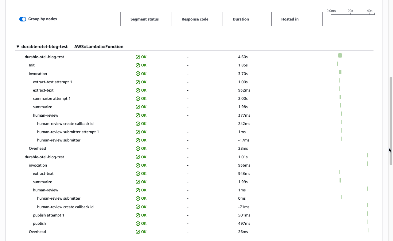
Figure 3. Trace details view. The service map shows the flow: Client to Lambda Context (first invocation), then Lambda Function (second invocation after callback resume). Both invocations appear under a single trace ID with total duration of 4.55 sec.
Correlated logs
Because the plugin sets enrich_logger=True by default, your application logs are automatically stamped with traceId and spanId.
Figure 4. Expanded log entry in CloudWatch. Each log record includes traceId, spanId, and otelTraceSampled set to true, which lets you correlate logs across all invocations of the same execution.
You can combine the plugin’s log correlation with structured JSON logging to run powerful queries in Amazon CloudWatch Logs Insights:
This returns logs from all invocations in chronological order, correlated to their respective spans.
Best practices
When you run the OTel plugin in production, keep the following performance, operational, and cost considerations in mind.
Performance considerations
- Cold start impact: The ADOT layer adds overhead to cold starts and memory consumption. Measure the impact for your workload using Lambda Power Tuning. For latency-sensitive functions, consider using provisioned concurrency to keep warm environments available.
- Memory overhead: The plugin and ADOT layer consume approximately 40–60 MB of additional memory. Verify your function has sufficient memory allocated.
- Replay efficiency: During replay, the plugin correctly identifies replayed operations and does not emit duplicate spans. Only new operations generate new spans.
Operational guidelines
- Name your operations: Always pass the
nameparameter tocontext.step(),context.wait_for_callback(), and other durable operations. These names appear as span names in your traces, making them human-readable. - Use structured logging: Combine the plugin’s log correlation with structured JSON logging to unlock powerful Amazon CloudWatch Logs Insights queries.
- Monitor trace gaps: If you see traces with missing spans, check that X-Ray active tracing is enabled and the ADOT layer is correctly configured.
Cost management
- Amazon CloudWatch Application Signals pricing: You are charged per trace recorded and per trace scanned. At high volumes, configure sampling to control costs. See Amazon CloudWatch Application Signals pricing.
- Log volume: With
enrich_logger=True, every log record includes trace context fields, slightly increasing log volume. This overhead is typically negligible but worth noting for high-throughput functions.
Pricing
The plugin is open source (Apache 2.0). Costs come from AWS X-Ray traces recorded and the ADOT Lambda layer overhead. The layer increases both the memory consumption and the cold start duration of your function. Lambda pricing is based on GB-seconds, so the additional memory allocated (rounded up to the nearest MB) multiplied by the additional execution time per invocation determines the cost impact. Each durable execution produces one trace regardless of invocation count, so X-Ray cost scales with executions, not invocations. Measure the overhead for your workload using Lambda Power Tuning and see AWS X-Ray pricing for current rates.
Beyond this post
This post focused on a single, representative workflow (sequential steps plus a human-approval callback) to keep the walkthrough concrete. It is not an exhaustive tour of the SDK. The Durable Execution SDK offers many other primitives that also produce spans and are worth exploring: durable timers (context.wait), condition polling (context.wait_for_condition), durable Lambda-to-Lambda calls (context.invoke), parallel and fan-out execution (context.parallel, context.map), nested child contexts, and automatic retries (with_retry and StepConfig), where each attempt and each parallel branch surfaces as its own span. We also did not cover failure paths, such as step errors and failure callbacks, which is where unified tracing is often most valuable.
Likewise, the OTel plugin exposes configuration we did not exercise here: toggling log enrichment (InvocationOtelPlugin(OtelPluginConfig(enrich_logger=False))), supplying a custom Tracer Provider via OtelPluginConfig(tracer_provider=...), and controlling trace volume through standard OpenTelemetry sampling (OTEL_TRACES_SAMPLER). This walkthrough sampled 100% of traces. Consult the SDK documentation for the full surface area, or access the GitHub repository.
Sending Lambda durable functions traces to Observability partners. The OpenTelemetry plugin exports telemetry data to Amazon CloudWatch and can work with any observability solution that supports OpenTelemetry. Dash0 is an OpenTelemetry-native observability platform that supports Lambda durable functions without custom configuration. Dash0 worked with AWS to validate the OpenTelemetry plugin for the AWS Durable Execution SDK for JavaScript prior to launch, Dash0 coordinates logs and spans. In Dash0, spans for the durable execution, each invocation, and each durable operation appear alongside the function’s inputs and outputs and the payloads of its AWS SDK calls. To learn more, visit About AWS Lambda Monitoring.
Clean up
To avoid ongoing charges, delete the resources created in this walkthrough:
This removes the Lambda function, AWS Identity and Access Management (IAM) roles, and any associated resources created by the SAM template.
If you manually added the ADOT Lambda layer or X-Ray tracing policies outside of your SAM template, remove those separately using the AWS CLI or console.
Trace data retained in X-Ray does not incur storage charges and expires automatically after 30 days.
Conclusion
In this post, we showed how to unify fragmented traces across multiple Lambda invocations using the OpenTelemetry plugin for the Durable Execution SDK. To explore the full SDK surface area, including parallel execution, durable timers, and failure-path tracing, see the AWS Durable Execution SDK Developer Guide. For more observability patterns, visit the AWS Observability Best Practices guide.
How Moonfrog scales analytics and lowers query cost with Amazon Redshift RG instances
Post Syndicated from Anirudh Chawla original https://aws.amazon.com/blogs/big-data/how-moonfrog-scales-analytics-and-lowers-query-cost-with-amazon-redshift-rg-instances/
Moonfrog Labs uses Amazon Redshift to analyze mobile game telemetry. Each session, purchase, and player drop-off generates events that product and analytics teams use to understand game performance. Faster loading and querying help those teams work with fresher data.
Moonfrog runs a single production analytics cluster with roughly 148 TB in Amazon Redshift Managed Storage (RMS) and about 4,000 warehouse tables. It also queries roughly 1,000 external data lake tables. The warehouse supports telemetry ingestion, revenue reporting, marketing attribution, and self-service dashboards for product, data science, analytics, and support teams.
In this post, we show how Moonfrog migrated its production analytics warehouse from Amazon Redshift RA3 to RG instances using elastic resize. We explain how the team selected capacity for growing analytics demand and more frequent loading, verified warehouse and data lake access, and assessed performance and costs after migration.
The challenge
Moonfrog’s RA3 cluster ran reliably, with no stability issues. Its constraint was compute headroom as analytics demand grew. Ingestion volume was steady before migration. Growth came from analytical queries and data lake scans. The team already planned to expand from five RA3 nodes to six or seven nodes and wanted capacity to load warehouse data more frequently.
The five-node ra3.4xlarge cluster averaged about 54% CPU utilization. In approximately 98% of hours, CPU peaked at or above 90%. Other indicators showed demand increasing:
- SELECT queries per day increased 31% from January to July.
- Mean workload management (WLM) queue wait for highest-priority queries rose from 505 milliseconds in May to 940.7 milliseconds in July.
- Concurrency scaling usage nearly doubled over the same period, from 4,453 to 8,516 seconds per day.
A COPY operation averaged 16.8 seconds on RA3. That duration constrained how often the stats pipeline could load. The team evaluated RG as a way to support growing analytics demand and make more frequent loads practical.
Moonfrog also queried roughly 1,000 external tables in Amazon Simple Storage Service (Amazon S3). Data scanned through Redshift Spectrum increased 33%, from 84.9 TB in March to 112.5 TB in June. The separate Spectrum scanning charge added to the cost of expanding RA3 compute.
Moonfrog used WLM query monitoring rules to stop scans larger than one terabyte. These rules controlled scan spend under the RA3 configuration.
The one-year no-upfront reserved node commitment for ra3.4xlarge expired in July 2026. Renewal gave Moonfrog an opportunity to re-evaluate its compute commitment and determine whether switching to RG would provide additional headroom for its growing workload needs.
Solution overview
Amazon Redshift RG instances use AWS Graviton processors and an integrated data lake query engine. AWS publishes benchmarks of up to 2.2 times faster warehouse workloads and up to 2.4 times faster Apache Iceberg workloads, at 30% lower price per vCPU than RA3. These benchmarks are separate from Moonfrog’s production results. RG runs Apache Iceberg and Apache Parquet scans on cluster nodes, removing the separate per-terabyte Spectrum charge for these scans. Elastic resize supports changing the node family and capacity without a customer-managed export and reload.
Moonfrog retained its ingestion and analytics architecture at cutover. No service was added or removed, and applications continued to use the same warehouse.
The following diagram illustrates the architecture.
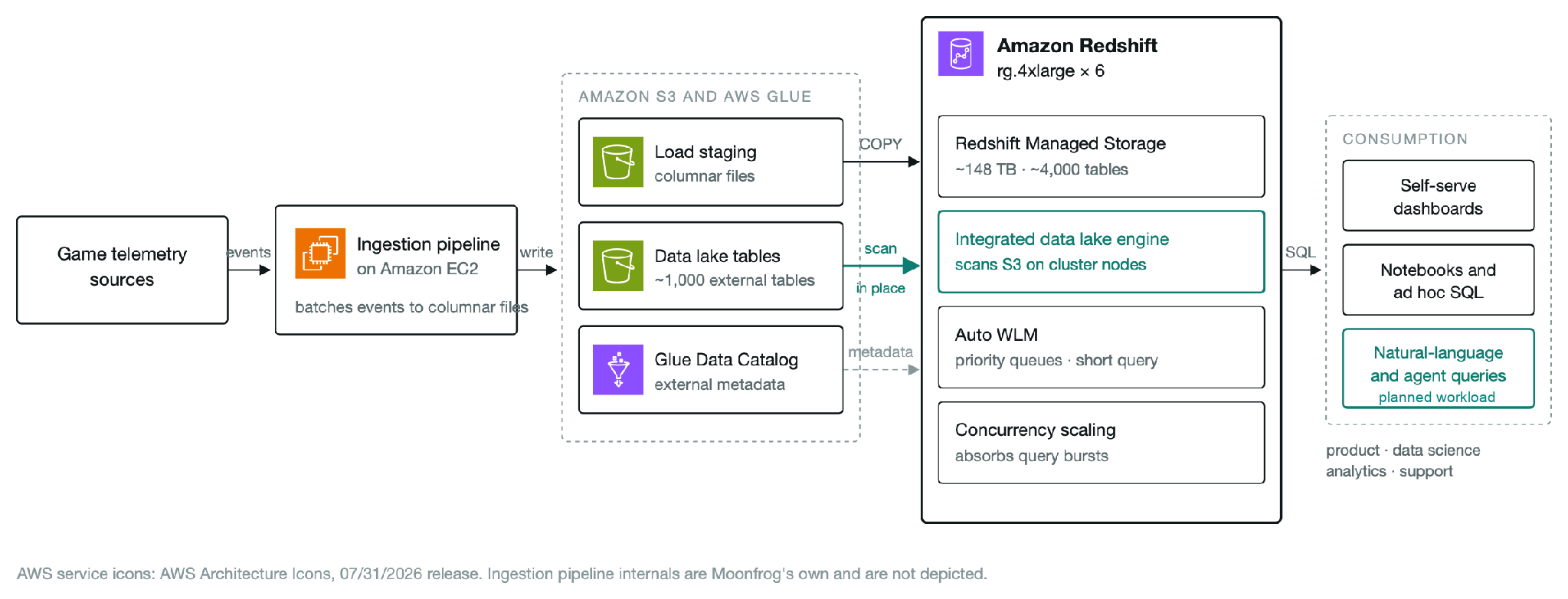
Figure 1: The ingestion pipeline writes columnar files to Amazon S3. COPY loads warehouse tables, and the integrated data lake engine on RG queries external tables in place. Conversational analytics is a planned use of the additional headroom
The architecture uses the following AWS services:
- Amazon Redshift provides the analytics warehouse and integrated data lake engine.
- Amazon S3 stores event files, load staging data, and external data lake tables.
- AWS Glue Data Catalog stores metadata for external schemas and tables.
- Amazon Elastic Compute Cloud (Amazon EC2) runs the ingestion pipeline.
- Amazon CloudWatch and AWS Cost Explorer provide performance and billing measurements.
Implementation steps
Moonfrog established a baseline, used elastic resize to change the node family, and verified warehouse and data lake access. It then evaluated the early results before selecting its final configuration.
Step 1: Establish a baseline
Before the change, the team captured Amazon CloudWatch metrics for CPU utilization, WLM queue wait by priority, query duration by type, and queries per day. COPY loads and SELECT queries were measured separately. Billing records provided reserved compute, Spectrum scanning, and concurrency scaling costs so the comparison covered each billing line affected by the move.
AWS provides migration planning and workload validation guidance in the AWS RA3 to RG best practices blog.
Step 2: Validate the target configuration and use elastic resize
AWS recommends testing the target RG configuration in a non-production environment with representative workloads before migrating production. That testing is intended to measure benefits, identify issues, and validate the target size before the production migration.
On 26 July, Moonfrog used elastic resize to move from five ra3.4xlarge nodes to eight rg.4xlarge nodes, temporarily providing extra capacity to reduce migration risk. It did not export or reload the 148 TB warehouse. Schemas, ETL jobs, application SQL, drivers, connection strings, and BI tools continued to work.
Amazon CloudWatch recorded one five-minute interval in which the cluster reported unhealthy. Database connections recovered immediately afterward. This sampling interval describes the observed impact. It does not establish an exact five-minute outage duration.
AWS guidance describes elastic resize as a short operation, typically about 10 to 15 minutes. After an RA3-to-RG node-type change, data hydration brings frequently accessed data from managed storage into the new nodes’ local cache. This cache warming should be considered when interpreting early performance measurements.
Step 3: Verify warehouse and data lake access
Moonfrog verified that warehouse loads and external queries continued after the resize. External schemas and tables remained in use, with AWS Glue Data Catalog providing their metadata.
Moonfrog confirmed that per-terabyte S3 scanning charges were eliminated for its RG queries in the subsequent billing records. Those queries used provisioned cluster capacity, which remained billable.
Step 4: Review workload management rules
Moonfrog’s Auto WLM configuration included separate queues for administrators, analysts, ETL, loading, and visualization, along with short query acceleration. These queues carried across the migration. The team reviewed query monitoring rules because data lake scans now consumed RG cluster capacity.
The review accounted for data lake scans sharing compute with warehouse workloads. Rules that previously controlled scan spend could still protect these shared resources.
Results and key benefits
The following four CloudWatch charts cover 1 May to 25 October 2026. Each marks the 26 July resize and shades the 26 July–3 August period when the cluster was reduced from eight to seven to six RG nodes. Query duration and WLM wait charts show seven-day rolling means. Query counts include COPY, SELECT, INSERT, utility, and other operations.
Stage 1: Evaluate RG after cutover
The first evaluation focused on workload continuity and query runtime. Warehouse loads and data lake queries continued, and the applications used the same schemas, SQL, drivers, and connection strings. Queries on the initial RG configuration were completing within expected runtimes. Moonfrog then reduced the node count in stages to assess whether each reduction affected query runtime.
The cleanest comparison of COPY duration is 27–31 July, when load volume remained unchanged. Mean duration fell from 16.8 seconds on RA3 to 3.6 seconds on RG, about 79% shorter. This window falls within the 26 July–3 August right-sizing period, before the final six-node configuration was established.
Select six nodes
Moonfrog reduced the cluster from eight to seven and then six RG nodes within eight days. The team retained the additional node relative to its five-node RA3 baseline to support growing analytical demand and more frequent loading. It had already planned to expand RA3 to six or seven nodes.
The move from five RA3 nodes to six RG nodes increased node count by 20%. Published node specifications list 12 vCPUs per ra3.4xlarge and 16 per rg.4xlarge, so provisioned vCPUs increased from 60 to 96, or 60%. The results reflect the change in both node family and capacity.
Stage 2: Sustain performance as workloads grow
After validating the available headroom on the six-node configuration, Moonfrog increased loading frequency on 24 August. The cluster now executes more than 70,000 COPY operations a day, about 4.3 times the RA3 baseline. These loads use smaller, more frequent batches, so later COPY duration also reflects the changed loading pattern. Figure 2 shows the early duration improvement and subsequent performance as the workload changed.
In late August, after the 24 August increase in loading frequency, Moonfrog purchased a one-year no-upfront reservation for the six-node RG configuration. The purchase followed its evaluation of RG with production traffic and committed capacity for anticipated workload growth.
Figure 2: Mean COPY and SELECT duration. The early COPY comparison uses unchanged volume. Later means also reflect smaller batches after 24 August
More daily queries with compute headroom
Daily queries across all types increased from around 49,122 on RA3 to 83,603 in August, 125,350 in September, and 125,374 during 1–25 October. From September onward, this was more than 2.5 times the RA3 baseline. COPY accounts for much of that increase, so total query growth should be read alongside the query mix in Figure 3.
Figure 3: Successful daily queries by type. COPY frequency increased on 24 August, after the migration and right-sizing period
Concurrency scaling remained enabled to absorb peak bursts alongside the six reserved nodes. Average daily usage was 14–29% below the RA3 baseline in August, September, and October, even as total query volume grew. Usage increased from September to October as demand rose.
Average CPU utilization fell from about 54% on RA3 to 35–39% from September onward, despite the higher query count. Figure 4 distinguishes daily average CPU from the typical peak, defined as the daily mean of each hour’s maximum CPU reading.
Figure 4: CPU utilization before and after the resize. The typical peak is an average of hourly maximum readings, not the single daily maximum
Queue waits as demand grows
Queue waits fell after migration and rose from their August lows as traffic increased in October. During 1–25 October, highest-priority waits averaged 561 milliseconds versus a July RA3 baseline of 940.7 milliseconds, and high-priority waits averaged 193 milliseconds versus 294 milliseconds. Normal-priority waits were about 11 milliseconds, above their July baseline of about 3.6 milliseconds. Figure 5 uses a separate vertical scale for each priority.
Figure 5: Seven-day rolling mean WLM queue wait by priority. Dashed lines mark July RA3 baselines. Each panel has its own scale
Integrated data lake queries and billing
External data lake queries continued after migration. Moonfrog confirmed that the separate Spectrum scanning charge remained exactly $0 from 27 July through the reported months:
- The Amazon Redshift system views showed that external queries continued. A recent three-day sample recorded roughly 200,000 external queries against Amazon S3, including Parquet scans. External schemas and tables remained in use.
- Billing records showed no separate per-terabyte scanning charge. External scans use provisioned RG capacity, which remains billable. Amazon S3 storage and other charges are outside this comparison.
Cost per query
Moonfrog chose additional capacity for growth, and monthly spend across reserved compute, Spectrum scanning, and concurrency scaling increased approximately 4–6%. On a consistent 30-day basis, cost per 1,000 total queries fell approximately 59% in September and 58% in October. Costs per 1,000 SELECT queries fell 38–50% across August through October.
| Metric | RA3 × 5 Before |
RG × 6 August |
RG × 6 September |
RG × 6 Oct 1–25 |
| Queries per day All types | 49,122 | 83,603 | 125,350 | 125,374 |
| Cost per 1,000 total queries | $5.60 | $3.45 −38% | $2.28 −59% | $2.33 −58% |
| Reported cost per 1,000 SELECT | $45.60 | $22.73 −50% | $25.19 −45% | $28.34 −38% |
Cost per 1,000 total queries is calculated by dividing the combined 30-day spend for reserved compute, Spectrum scanning, and concurrency scaling by 30 times the average daily query count, then multiplying by 1,000. These are aggregate cost measures, not the execution cost of an individual query.
How the team plans to use the headroom
The larger configuration created room to test additional analytical use cases. Earlier measurements showed mean short-query duration falling from about 2.8 seconds to 1.8 seconds. That observation applies to the measured short-query workload and does not establish a response-time guarantee for every analytical question.
Moonfrog plans to evaluate conversational analytics using large language model (LLM) agents. Such agents may execute several queries to answer one question, so query latency is one part of the end-to-end response time. The additional compute headroom gives the team room to test these workloads alongside existing analytics.
Lessons learned
- Use a reserved node renewal as an opportunity to review capacity and architecture for your growing workload needs. Moonfrog evaluated RG before making another one-year commitment.
- Size the cluster for expected workload growth and assess results against the capacity provisioned. Moonfrog added a sixth node for headroom. Interpret total query counts alongside the query mix, because smaller, more frequent COPY batches increase the number of operations.
- Include concurrency scaling in capacity planning. In this deployment it continued to absorb peak bursts alongside the reserved nodes, so evaluate its contribution when assessing warehouse throughput.
- Separate immediate migration results from subsequent workload changes. The unchanged-volume COPY comparison captures the first days after cutover. Later results include the loading cadence change and rising demand. Measure dashboard latency and query abandonment separately to quantify the effect on users.
Next steps
Moonfrog has already increased warehouse loading frequency. The team plans to measure dashboard load times and query abandonment to assess how greater freshness and shorter query durations affect the experience of product and analytics teams.
Moonfrog is considering Apache Iceberg for data lake tables currently stored as Parquet files. The table format would add capabilities such as schema evolution and time travel. The team will evaluate these changes alongside performance and operating requirements.
The team also plans to evaluate broader natural language access. Governance must define which teams can access each table and how exploratory queries share cluster resources. End-to-end agent response time will need separate measurement.
Conclusion
Moonfrog migrated its 148 TB production Amazon Redshift warehouse from five RA3 nodes to RG using elastic resize, then settled on six nodes after eight days of measured right-sizing. RA3 had run reliably. The change addressed growing analytics demand and the need for more frequent warehouse loads. COPY duration fell from 16.8 seconds to 3.6 seconds at unchanged volume immediately after cutover.
With six RG nodes, Moonfrog handled more than 125,000 daily queries across all types from September onward, over 2.5 times the RA3 baseline. Average CPU utilization was 35–39%. More frequent COPY batches contributed to the change in query mix. External queries continued with no separate Spectrum scanning charge, and concurrency scaling provided burst capacity alongside the reserved nodes.
To evaluate RG for your warehouse, review Amazon Redshift pricing, the elastic resize documentation, and the RA3 to RG migration best practices. Establish a baseline and test representative workloads in a non-production environment first. Validate warehouse and data lake access, then compare total spend and cost per unit of work before committing to reserved capacity.
About the authors
Monitor the efficiency and availability of accelerated computing instances with Amazon EC2 Detailed Monitoring and performance status checks
Post Syndicated from Caroline Frost original https://aws.amazon.com/blogs/compute/monitor-the-efficiency-and-availability-of-accelerated-computing-instances-with-amazon-ec2-detailed-monitoring-and-performance-status-checks/
Amazon Elastic Compute Cloud (Amazon EC2) accelerated computing instances run some of the most demanding workloads customers operate, from large model training and distributed fine-tuning to high-throughput, live inference. These customers seek high availability and performance to make sure their training and inference run efficiently. To meet their performance goals, customers require visibility into the efficiency and performance of each accelerated computing chip in their fleet.
For example, central infrastructure or machine learning teams often operate accelerated computing capacity for many application teams. These infrastructure teams need a clear view of utilization and health across every instance in their fleet even if they don’t develop the applications running on those instances. They are often responsible for how efficiently that capacity is used and for hardware health, while application teams own the workload. Customers asked us to provide foundational telemetry for their accelerated computing efficiency and status that doesn’t require setup within the instance and complements their in-guest tooling.
Amazon EC2 now reports one-minute graphics processing unit (GPU) metrics through Detailed Monitoring and surfaces recoverable conditions with performance status checks. One-minute GPU metrics in Amazon EC2 Detailed Monitoring report per-GPU utilization and thermal data to Amazon CloudWatch, so you can identify underused capacity and tune workloads for cost and throughput. Performance status checks report recoverable hardware conditions, such as a GPU memory error, to help you manage GPU performance.
Feature overviews
Amazon EC2 reports GPU metrics and performance status checks without an in-guest agent and without using instance compute. These capabilities are available on supported NVIDIA GPU-based accelerated computing instance types. For the metrics supported on each instance family, see the Amazon EC2 Detailed Monitoring documentation.
One-minute accelerated computing metrics extend EC2 Detailed Monitoring and are published to CloudWatch as OpenTelemetry Metrics or CloudWatch Metrics. The metric name you add to a category determines which one CloudWatch publishes: include GPUUtilization for a CloudWatch Metric, instance.gpu.utilization for an OpenTelemetry Metric, or both names to publish both. Amazon EC2 publishes each metric to CloudWatch at two levels: one series for the instance, identified by InstanceId, and one series for each GPU, identified by InstanceId and GpuId. GpuId is the GPU UUID, which you can match to a device by running nvidia-smi -L on the instance.
Performance status checks add a fifth status check to the existing Amazon EC2 product check suite of system, instance, attached EBS, and application status checks. The check reports recoverable hardware issues that affect accelerated computing performance while the instance might remain running and reachable. It surfaces through the EC2 console, through DescribeInstanceStatus, and in CloudWatch metrics.
Evaluating accelerated computing utilization and performance with EC2 Detailed Monitoring
Amazon EC2 Detailed Monitoring reports per-GPU measurements, including compute activity, memory use, temperature, and data movement.
GPU utilization metrics report different aspects of GPU use. GPUPowerUtilization is available by default and reports active power use. Power utilization scales with the depth of work the GPU performs. Compare it with more granular utilization metrics to see how efficiently your workload uses the GPUs. GPU utilization shows the percentage of time the GPU was running work. Because a busy GPU might use only a fraction of its streaming multiprocessors (SMs), compare it with SM utilization to see how much of the compute capacity the workload uses. Memory utilization shows how much of the GPU’s memory capacity is in use, helping you assess memory headroom. Context accumulated time is a running total of the time a process has held the GPU open, whether or not it ran work. Use the CloudWatch metric math expression RATE(m1)/1000000, where m1 is GPUContextAccumulatedTime, to compare context activity with GPU utilization. A result close to 1 with low GPU utilization indicates that a GPU context is held open but idle.
GPU temperature is reported as a percentage of the GPU’s thermal throttle limit, and memory temperature as a percentage of the memory’s critical temperature. Both metrics can report values above 100 percent when a GPU or its memory runs above the limit. A GPU reduces its clocks when it reaches its throttle limit, so a value at or above 100 percent can explain a drop in throughput. You can correlate these measurements with GPU and interconnect utilization metrics to understand workload performance.
Interconnect utilization metrics show how much of the available bandwidth a workload uses for data movement. Each value reports the busier direction, either send or receive. NVLink utilization measures GPU-to-GPU traffic, such as collective operations in distributed training. It reports all of the GPU’s links together. PCIe utilization measures traffic between the host and the GPU.
Getting started with EC2 Detailed Monitoring
Amazon EC2 Detailed Monitoring publishes instance metrics to Amazon CloudWatch at one-minute intervals without running an agent in the guest operating system. You can publish these as OpenTelemetry Metrics or CloudWatch Metrics.
To get started, create a metric category, an Amazon EC2 resource containing the metrics you want to collect. Next, associate the category with one or more instances. For an existing instance, provide the category ID when you enable Detailed Monitoring with the MonitorInstances API. For a new instance, provide the category ID in the Monitoring object when you call RunInstances or configure a launch template.
The following example creates a metric category for GPU utilization, SM utilization, and memory utilization.
The response includes a metric category ID. To associate the category with an existing instance, use MonitorInstances.
To associate the category when you launch an instance, include the category ID in the Monitoring object.
To apply a category to every instance launched from a launch template, include the category ID in the Monitoring object in the launch template data.
Categories apply to many instances at once, unlike per-instance metric settings. Define the metric set once and associate it wherever it applies. Every associated instance then reports the same set of metrics. Changing a category updates the metric set for every associated instance. The change is eventually consistent across running instances. Add the category to a launch template to apply the same metrics to new instances. This gives you one metric definition per workload type instead of one configuration per host. Metrics apply under standard Amazon CloudWatch pricing.
Managing accelerated computing availability with performance status checks
Accelerated computing hardware can experience non-terminal issues that affect performance and can be resolved with a GPU reset or an instance reboot. For example, when a GPU encounters an uncorrectable memory error, it schedules a repair that remaps the affected row to a spare. The repair takes effect the next time the GPU is reset or the instance is rebooted.
Amazon EC2 performance status checks surface these recoverable hardware conditions. For example, when Amazon EC2 detects a pending GPU memory row remap, the instance’s performance status check reports an impaired status and identifies reboot as the recommended remediation.
You can view performance status checks on the Amazon EC2 console or through DescribeInstanceStatus. Amazon EC2 also publishes the StatusCheckFailed_Performance metric to CloudWatch. A failed performance status check also increments the combined StatusCheckFailed metric. The following example uses the EC2 DescribeInstanceStatus API:
The following response shows the system, instance, attached EBS, and configured application status checks passing while the performance status check is impaired:
Amazon EC2 sends a scheduled event for the instance if the condition requires further action after a reboot.
To act on these conditions across your accelerated computing instances, create a CloudWatch alarm on StatusCheckFailed_Performance.
- The alarm on
StatusCheckFailed_Performancefires for an instance in a training cluster. - You confirm the condition and the recommended action with
DescribeInstanceStatus, which returns a status of impaired and a remediation of reboot. - You checkpoint the job if applicable, then drain the node and reboot the instance at a planned point. On Amazon Elastic Kubernetes Service (Amazon EKS), cordon and drain the node. In Slurm, set the node to
DRAIN. - After the reboot completes, the performance status check returns to ok.
The following command creates that alarm for a single instance.
A CloudWatch Metrics Insights alarm evaluates a single query across all matching instances, so one alarm can cover a large fleet. To drive automation without an alarm, poll the DescribeInstanceStatus API.
Rebooting the instance is the recommended remediation. Alternatively, you can reset the affected GPU while keeping the other GPUs running. On the affected instance, run nvidia-smi -q -d ROW_REMAPPER and find the GPU that reports Pending: Yes. Stop all processes using that GPU, then use root permissions to run nvidia-smi -r -i <GPU_UUID>. The performance status check returns to ok shortly after the reset completes.
Bringing it all together
Accelerated computing metrics and performance status checks address complementary questions. Detailed Monitoring metrics help you find idle or underused capacity and tune workloads for cost and throughput. Performance status checks surface recoverable conditions and recommend remediation. Together, these EC2 signals report utilization and status across the capacity infrastructure teams manage, while in-guest tooling provides workload-specific analysis.
For example, a central infrastructure team monitors how efficiently workloads use the accelerated computing instances it manages for several application teams. It finds that one team’s GPUs report lower GPU utilization and power utilization than comparable workloads run by other teams. The infrastructure team shares the finding and relevant workload-tuning practices with the application team. After the application team updates that workload, the infrastructure team uses the same CloudWatch metrics to evaluate the change. The infrastructure team also monitors StatusCheckFailed_Performance across the fleet. When a check reports an impaired status and recommends a reboot, the orchestrator saves the active job, stops placing new work on the instance, and reboots it. After the check returns to ok, the orchestrator makes the instance available for new jobs. Together, these workflows help the team improve GPU utilization, protect job progress, and return affected capacity to service.
Amazon EC2 Detailed Monitoring reports accelerated computing metrics once per minute at the instance and GPU levels. Performance status checks report recoverable conditions at the instance level. Infrastructure teams can use these EC2 signals to monitor utilization and status across the capacity they manage. In-guest tools add process, container, Kubernetes pod, and sub-minute detail.
Amazon EC2 Detailed Monitoring reports metrics for your instances, including GPU utilization metrics reported per GPU. Performance status checks tell you when accelerated computing hardware needs attention. These capabilities help you evaluate utilization and manage the efficiency of your accelerated computing fleets. To learn more, see the Amazon EC2 Detailed Monitoring documentation and the EC2 status checks documentation.
About the author
Guardrails and cost control for your agentic workloads with Amazon Redshift
Post Syndicated from Jason Pedreza original https://aws.amazon.com/blogs/big-data/guardrails-and-cost-control-for-your-agentic-workloads-with-amazon-redshift/
Note (November 2026): This post covers both MCP servers because the Redshift MCP Server has Redshift-specific settings, such as read-only by default and a cap on result rows, that the AWS MCP Server doesn’t have yet. We’ll update this post when the AWS MCP Server reaches parity.
Guardrails and cost control matter more as AI agents handle an increasing share of the queries in your analytics environments. Asked “Why did revenue drop in the West region last weekend?”, an agent finds the tables, writes and runs the SQL on Amazon Redshift, and follows up. This is agentic analytics, on your data warehouse and lakehouse.
Two risks decide whether these agentic workloads reach production. The OWASP Top 10 for LLM Applications names both:
- Excessive agency: The agent can do too much. An agent acts on what a model decides. With more tools or permissions than its task needs, a misread request or an instruction hidden in a support ticket can become a real action, such as exporting customer records.
- Unbounded consumption: The agent can spend too much. A retry loop can rerun a heavy query all night. A query can return millions of rows that the agent then sends to the model as input tokens. Finally, one SQL query that runs Amazon Bedrock model inference through Redshift ML invokes the model once for every row it processes.
Redshift includes the controls for both at no additional charge: per-agent roles, row-level and column-level security, dynamic data masking, read-only tools, workload management, and usage limits. You pay for queries from agents as you do for queries from any other client: for the compute and storage they use (Amazon Redshift pricing). Your agent’s model provider bills its model tokens, for example at Amazon Bedrock pricing when the agent uses a model in Amazon Bedrock. You pay for the Amazon Bedrock, Amazon Bedrock AgentCore, and monitoring controls in this post at their own rates.
In this post, we show you how to add guardrails and cost controls to agentic analytics on Redshift, using one model: six guardrails, three enforcement layers, and one cost envelope.
The layered guardrail model
Each request passes through the agent layer, the access layer, and the data layer before it reaches your data warehouse or lakehouse, and the cost envelope limits spend across them.
Figure 1: The layered guardrail model. The lower the layer, the less a prompt can change it
Each guardrail type controls one thing and maps to an OWASP risk. Each layer is who enforces it:
- Agent layer: Your agent or application, its framework, and Amazon Bedrock.
- Access layer: The tools between the agent and your data, such as MCP servers and AgentCore Gateway (a capability of Amazon Bedrock AgentCore), and the IAM policies on the identities those tools use.
- Data layer: Amazon Redshift and, for lakehouse tables, AWS Lake Formation.
The following table lists the six guardrail types. Each row names the guardrail type, the main OWASP risk it reduces, and the layer and controls that enforce it.
| Guardrail type | Main risk (OWASP) | Who enforces it |
| Input | Prompt injection (LLM01) | Agent layer: Bedrock Guardrails, input validation |
| Reasoning and planning | Excessive agency (LLM06) | Agent layer: skills, business context, tool allow lists, step limits |
| Tool and action | Excessive agency (LLM06) | Access layer: tools, IAM, Policy in Amazon Bedrock AgentCore, threshold approval |
| Data | Sensitive information disclosure (LLM02) | Data layer: privileges, row and column policies, masking |
| Output | Sensitive information disclosure (LLM02), Improper output handling (LLM05) | Data layer. Agent layer for answers |
| Runtime and cost | Unbounded consumption (LLM10) | Data layer limits, token caps, AWS Budgets |
The agent layer is the first filter, but it cannot be the only one. Most Amazon Bedrock Guardrails checks are model-based classifiers, some with a strength that you tune, so they catch most problems but not all. The guardrails that protect your data in Redshift therefore sit in the access and data layers, which apply fixed rules to the caller’s identity. You need both. AWS Identity and Access Management (IAM) policies decide which Redshift workgroups and APIs it can call, and Redshift and Lake Formation permissions decide what its SQL can touch. Fixed rules give the same answer whichever agent wrote the request, so a prompt injection that gets past the agent layer still cannot reach data that the agent’s identity is not granted.
Agentic analytics patterns on Amazon Redshift
Conversational analytics, the most common pattern, answers business questions from your data in self-service and managed delivery models. The others enrich data, take actions, or help administrators run the warehouse itself.
| Pattern | How it connects to Redshift | Starting agency |
| Conversational analytics, self-service | AI assistants (agents that a person works with directly) such as Kiro, Amazon Quick, and the Amazon SageMaker Data Agent, through the AWS MCP Server or Amazon Redshift MCP Server over the Redshift Data API | Read-only |
| Conversational analytics, managed | Amazon Bedrock Knowledge Bases turns end users’ questions into SQL | Read-only |
| Enrich | Redshift ML with Amazon Bedrock calls a model from SQL | None: the model returns a column value |
| Act | One scoped tool per action | Scoped writes. Human approval for consequential ones |
| Operate | Administrators review and tune the warehouse with Kiro, Redshift skills, and the MCP Server review_cluster tool |
Read-only. Changes ship as reviewed code |
Every pattern needs the same two scopes for least privilege: IAM permissions that limit which workgroups and APIs an identity can call, and database permissions that limit what its SQL can read or change. What differs is which identity reaches Redshift:
- Self-service (AI assistants with the Redshift MCP Server or AWS MCP Server). The AI assistant acts on behalf of the user, with the AWS profile in its MCP configuration. If your roles have different scopes, set up a profile for each and point the server at the narrowest one for the task, such as a read-only analyst role for sales questions. The setup steps are in access-layer/redshift-mcp-server and access-layer/aws-mcp-server in the aws-samples repository.
- Redshift MCP Server: A user whose profile assumes a DataPlatformAdmin role runs every agent query as
IAMR:DataPlatformAdmin, with that role’s grants. The server is read-only by default, and the agent can’t switch profiles. To use a broader profile, change it yourself in the MCP configuration. - AWS MCP Server: The agent can switch on each call among the profiles listed in the MCP Proxy for AWS configuration. List only the profiles you want it to use, and put the read-only one first so it’s the default. On provisioned clusters, a script can also choose a database user if the role allows
redshift:GetClusterCredentials, so leave that permission out. - Both: The MCP configuration only controls the MCP tools. An agent that can run shell commands can use any profile on the machine, so the IAM roles and database grants are the real boundary.
- SageMaker Data Agent: The agent runs SQL itself, including cells it fixes, as the signed-in person. Without trusted identity propagation, Redshift sees one
IAMR:user-<id>@<project>database user per project member. With it, Redshift sees the person’s AWS IAM Identity Center user, so row-level security, masking, and grants apply to each person.
- Redshift MCP Server: A user whose profile assumes a DataPlatformAdmin role runs every agent query as
- Custom agents, for example on Amazon Bedrock AgentCore. The database user comes from the role that calls the Data API: the AgentCore Runtime execution role, or the AWS Lambda function’s role behind AgentCore Gateway, such as
IAMR:agent-support. If the agent acts for a specific person, use trusted identity propagation. The agent’s tool exchanges the person’s sign-in token through AWS IAM Identity Center, optionally federated with your external identity provider, and calls the Data API as that person. Redshift then applies their grants (writes included), row-level security, and masking, plus Lake Formation permissions if you enable that integration. - Managed (Amazon Bedrock Knowledge Bases). The knowledge base runs the SQL it generates as one identity. On Serverless workgroups and provisioned clusters, that is its service role with IAM or the user in an AWS Secrets Manager secret. Provisioned clusters also accept a named database user (authentication methods). Knowledge Bases can’t carry the actual user with trusted identity propagation, so when one identity serves many end users, row-level security can’t tell them apart. With one shared knowledge base, a West region manager and an East region manager query as the same database user, so both get every row that user can read. Instead, create one knowledge base or agent for each audience, such as one per sales region, and scope its role, grants, and row-level security policy to that audience.
Figure 2: Who Redshift sees on each access path
Decide how much agency to grant
Grant agency, what an agent can do, on two planes. The data plane is SQL on Redshift managed storage or Apache Iceberg tables, governed by Redshift and AWS Lake Formation permissions. The control plane is API calls that create, resize, manage, or delete infrastructure, governed only by IAM. The AWS Agentic AI Security Scoping Matrix bounds agency with permissions and autonomy with oversight. Following it, start read-only (Scope 1), then add scoped writes with a human in the loop for consequential ones (Scope 2). Keep agents off the control plane, and widen autonomy (Scopes 3 and 4) only within those boundaries.
Agent layer: Guide the request
The agent layer, mostly outside Redshift, is the first filter. Its controls run in your agent, Amazon Bedrock, and Amazon Bedrock AgentCore, so you set them up and pay for them there. These include the step, retry, and token limits that cap the agent’s own model spend.
- Input. Bedrock Guardrails filters prompt injection attempts and denied topics, and ApplyGuardrail works with your choice of model.
- Skills. The redshift-guide skill gives agents Redshift-specific knowledge, so fewer queries fail. The Agent Toolkit for AWS (
aws configure agent-toolkit, AWS Command Line Interface (AWS CLI) 2.35.0 or later) and the AWS Data Analytics Plugin deliver skills to Kiro and other AI assistants. - Business context. Business context and skill assets in the AWS Glue Data Catalog tell agents which tables and joins to use. They are in preview in the US East (N. Virginia), US East (Ohio), US West (Oregon), and Europe (Ireland) Regions.
- Agent configuration and oversight. Limit an agent’s tools before it runs. In Kiro, for example, the MCP configuration lists the tools to approve automatically (
autoApprove) and the tools to hide from the agent (disabledTools). Add project instructions, and set step and retry limits in agent frameworks.
Access layer: Limit what the agent can call
The access layer decides which tools an agent can call and what each call can do. Redshift enforces its guardrails the same way for every prompt.
Data plane: A narrow tool surface on every path
Figure 3 shows the tool guardrail each connection path needs, plus least-privilege IAM and database permissions. Each path has a worked example in the access-layer folder of the aws-samples repository, with setup, verification, and clean-up steps.
Figure 3: Access paths and their guardrails
Agents with shell access can bypass an MCP server with the AWS CLI, so scope IAM on every path. To allow only the AWS MCP Server path, see AWS MCP Server only, later in this section.
The agent’s IAM policy, access-layer/shared/agent-data-plane-policy.json in the aws-samples repository, has three statements:
- Discover lets the agent list workgroups. It uses
"Resource": "*"becauseListWorkgroupsdoesn’t support resource-level permissions, so it can’t limit where SQL runs. - RunSqlOnOneWorkgroup lets the agent sign in and run SQL on one workgroup only. This is the statement that limits where SQL runs. It includes
redshift-data:BatchExecuteStatement, which the Redshift MCP Server needs before it can run writes or named transactions. Without that action, the server stays read-only by refusing writes itself. With it, writes still needACCESS_MODE=read-writein the MCP configuration, which is off by default, and the agent’s database grants still limit what a write can change. - ReadOwnStatements lets the agent check status and read results only for statements it ran itself.
Custom MCP server: Tools that run fixed SQL. Expose only tools that each run one fixed, parameterized statement against a curated view, under the server’s own IAM role with SELECT on that view only. Have each tool set a fixed StatementName and SQL comment, so AWS CloudTrail and query history name the tool. In the sample server (access-layer/custom-mcp-server/sales_metrics_mcp.py), the agent supplies only a sales region, which the server checks against an allowed list, so prompt injection can at most make the tool query a different allowed region.
AWS MCP Server: Scope the credentials, not the script. Its aws___run_script sends SQL through the Data API as the caller’s mapped database user, so an administrator profile means administrator access. Four guardrails close that gap:
- A dedicated agent profile in the MCP Proxy for AWS, for an agent role with read-only grants.
- No way to switch database users. Allow
redshift-serverless:GetCredentialsorredshift:GetClusterCredentialsWithIAM, notredshift:GetClusterCredentialsor Secrets Manager secrets, which let a caller choose another user. - Agent workgroups only. A service control policy in AWS Organizations denies Data API SQL through AWS managed MCP servers unless the workgroup is tagged
agent-access=true. The same statement also works in an IAM policy or permissions boundary. SCPs skip the management account, so test on a sandbox OU first:
- AWS MCP Server only. To stop the agent’s shell from going around the server, deny
redshift-data:*on the agent role unless the call comes through it. Also deny direct driver sign-in whenaws:ViaAWSServiceis false:redshift-serverless:GetCredentials,redshift:GetClusterCredentialsWithIAMandredshift:GetClusterCredentials, plusGetIdentityCenterAuthTokenwhen you use trusted identity propagation (access-layer/aws-mcp-server/deny-data-api-outside-aws-mcp.json). Attach it to agent roles or permission sets, not as an SCP. IAM can’t tell the local Redshift MCP Server from the AWS CLI, so on that path read-only database grants are the boundary:
Bedrock Knowledge Bases: One database, listed tables, read-only grants. Inclusions (up to 50 tables) and exclusions narrow the generated SQL but aren’t a substitute for guardrails. A timeout of up to 200 seconds (60 in access-layer/bedrock-knowledge-base/kb-redshift-config.json) cancels the query. Scope the service role to one workgroup (and redshift-serverless:GetCredentials on Amazon Redshift Serverless) with SELECT on included tables only. Allow DescribeStatement, GetStatementResult, and CancelStatement on its own statements only. The sync fails without CancelStatement (access-layer/bedrock-knowledge-base/kb-service-role-policy.json).
Scope every write, and keep a human in the loop where it matters
Give an agent one scoped tool per action, never a generic write tool. A write can run on its own when its tool limits it to one validated, low-impact action, so approvals don’t slow routine work. Consequential, irreversible, or above-threshold writes need a human in the loop:
| Mechanism | How it works | Can the agent bypass it? |
| Approve as data (recommended for data writes) | The tool records a request. A people-only identity approves it | No: Redshift enforces it |
| Approve in the agent | The framework asks a person first | Depends on the framework |
| Approve as code review | Schema and infrastructure changes ship as reviewed code | No: your pipeline enforces it |
In the Act pattern, an agent writes to Redshift as part of a workflow, such as issuing a refund. Figure 4 shows how it combines both kinds of write:
- The agent’s only write tool,
refund_order, runs as an identity that can onlyEXECUTEone procedure. - The SECURITY DEFINER procedure checks the order and caps the amount at the remaining refundable amount and $500, locking
support.refundsagainst concurrent over-refunds. A failed check writes nothing and returns an error the agent can report. - Refunds up to $100 are approved. Larger ones wait for the
refund_approversrole, through a second procedure that rejects self-approval. - A payment process pays approved refunds only.
Figure 4: A scoped action tool, with human approval above a threshold
The procedures and grants are in act-refund/refund_procedures.sql. Expose refund_order as its own tool, under an identity separate from the agent’s read path, so the read identity has no write privileges. Scheduled writes that no agent starts, such as a nightly Enrich job that labels tickets with Redshift ML, need a different control. Review the job’s SQL once before you deploy it, then run it under its own identity that no agent can use.
Control plane: Keep infrastructure changes out of agents’ reach
Control plane calls skip database grants, so IAM is the only gate, and an AI assistant’s credentials often reach its shell and the AWS CLI too.
Give every AI assistant a scoped identity. Run Kiro and other AI assistants, and their MCP servers, under an agent-role AWS profile with read-only control plane actions and a permissions boundary. Don’t allow redshift:Get*, which includes GetClusterCredentials. Share the profile through one AWS IAM Identity Center permission set (access-layer/shared/aws-config-example.ini). Role chaining caps sessions at 1 hour.
Deny infrastructure changes through managed MCP servers. With the aws:ViaAWSMCPService condition key, a service control policy can deny create, delete, modify, resize, pause, resume, reboot, restore, and tagging actions made through an agent but not directly (access-layer/shared/deny-infra-changes-through-agents.json). Tagging matters because the data plane deny trusts the agent-access tag.
Data layer: Decide what the agent can reach
The data layer decides what an agent can actually reach, on every query. As the Redshift MCP Server documentation puts it, “The database user’s privileges are the security boundary, not this server.”
Give every agent its own identity: One IAM role, database user, and database role. The IAM role agent-support signs in through the Data API as IAMR:agent-support. On Redshift Serverless, a RedshiftDbRoles tag can grant its database role at sign-in (the aws-samples repository shows the tag). Agents acting for a person can use trusted identity propagation. Grant the role after the user’s first sign-in:
Then narrow what it sees (data-layer/fine-grained-access.sql):
- Row-level security (RLS) filters rows only on tables you attach it to and makes a table default-deny, so attach policies for other roles first.
- Column privileges remove columns, such as email.
- Dynamic data masking transforms values, such as a card’s last four digits.
Limit what agents can discover. Turn on metadata security so catalog views and SHOW list only objects the role can access, so agents cannot plan around hidden tables (superusers and ACCESS CATALOG roles see all). Test on non-production first:
Extend the rules to the lakehouse and other warehouses, so no path skips your filters. Redshift enforces Lake Formation permissions on Iceberg tables, including Amazon S3 Tables (a capability of Amazon S3), and federated permissions carry RLS and masking to an agent warehouse. Plain datashares do not carry RLS filters.
Treat free text as untrusted: Keep Redshift ML instructions in the static PROMPT prefix, and pass row text only as input.
Allow only approved models. The model’s IAM role decides at inference time, so allow bedrock:InvokeModel only on approved model ARNs. By default only superusers can create models. Grant CREATE MODEL to an ML platform role, with ASSUMEROLE ... FOR CREATE MODEL only on approved IAM roles.
Audit each agent’s reach with HAS_TABLE_PRIVILEGE (observe/detection/agent-table-privileges.sql). Until you revoke the default PUBLIC ASSUMEROLE grant, assume every user can use every IAM role attached to the warehouse. The AWS Identity and Access Management Access Analyzer (IAM Access Analyzer) check-access-not-granted check can fail deployments that grant redshift:GetClusterCredentials.
Test as the agent: Superusers and sys:secadmin bypass RLS.
Output guardrails: What the agent sees, keeps, and says
An agent has three outputs: results it reads, copies it keeps, and its answer. Redshift controls what enters the agent and its database-side copies. The application and agent layer govern the rest.
What the agent sees and says
The data layer’s policies double as output guardrails: results hold only permitted rows and readable columns, masked values stay masked, and Lake Formation filters do the same for Iceberg tables.
The sensitive information filtering in Bedrock Guardrails doesn’t inspect toolResult content, so mask in Redshift.
Cap result size too: provisioned clusters can abort on return_row_count, and the Redshift MCP Server’s MAX_RESULT_ROWS (1,000 by default) refuses larger results, protecting the context window, not compute.
Data-layer controls end when results leave Redshift, so check the answer too: Bedrock Guardrails can mask PII and flag ungrounded answers, and the generated SQL makes the answer traceable.
What the agent keeps: Database-side exports and copies
A copy starts with none of the source table’s policies, so treat every database-side write path as an output path:
| Export path | Guardrail |
UNLOAD to Amazon S3 |
REVOKE ASSUMEROLE ON ALL FROM PUBLIC FOR ALL (which also blocks COPY and CREATE MODEL). Grant ASSUMEROLE ... FOR UNLOAD to pipeline roles only |
CETAS and INSERT into external tables |
Agent roles own no external schemas |
| Writes to Apache Iceberg tables | No Lake Formation write permissions for agent-facing roles |
CTAS, SELECT INTO, and INSERT ... SELECT |
REVOKE CREATE ON SCHEMA public FROM PUBLIC. No CREATE or INSERT for agents |
| Datashares | No datashare privileges for agent roles |
The MCP Server’s read-only mode denies UNLOAD and CALL, but other paths bypass it, so privileges are the durable line (data-layer/exports-and-copies.sql). Audit exports in SYS_UNLOAD_HISTORY, SYS_QUERY_HISTORY, and CloudTrail S3 data events.
Figure 5 summarizes which layer controls each output.
Figure 5: What the agent sees, keeps, and says, and which layer controls each
The cost envelope: Predictable by design
Each agent question has three cost parts (Figure 1): model tokens at Bedrock rates, query compute on Redshift provisioned clusters or Amazon Redshift Serverless RPUs that you already pay for (older RA3 and DC2 clusters also bill lakehouse scans per terabyte), and data at rest. These compute guardrails are part of Redshift, and you pay only for the Redshift compute your queries use:
| Guardrail | Provisioned | Serverless |
| Separate lane for agents | WLM queues by user role | Queues by user role, or a dedicated workgroup |
| Stop a runaway query | Query monitoring rules that log, hop, or abort | Workgroup query limits or queue rules that log or abort |
| Cap each statement | statement_timeout per agent user |
Same as provisioned |
| Cap connections | CONNECTION LIMIT and SESSION TIMEOUT per agent user |
Same as provisioned |
| Cap capacity | Fixed node count. Concurrency scaling limits | Max capacity in RPUs |
| Cap spend per period | Concurrency scaling and Spectrum limits | RPU-hour limits per day, week, or month |
Set three ceilings on day one (Figure 6): a per-statement timeout for each agent user, max capacity on the agent workgroup, and a daily usage limit. Queue rules are checked every 10 seconds, so the timeout is the tighter cap.
Figure 6: The cost envelope. Each ceiling catches what the one inside it misses
Max capacity and the usage limit do different jobs (see Billing for on-demand compute capacity). Max capacity caps RPUs. The usage limit logs, alerts, or stops user queries once the period’s RPU-hours are used (cost-envelope/serverless-ceilings.sh). emit-metric only publishes a metric. Alarm on it, or choose Alert on the AWS Management Console.
Each Serverless workgroup or RG cluster accepts at most 2,000 connections. In our tests, Data API tools opened one connection per call, but an idle open driver transaction kept Serverless compute running until the 1-hour timeout. On Serverless, deny redshift-serverless:GetCredentials when aws:ViaAWSService is false. In our tests, this blocked driver sign-in, not direct Data API calls. On each non-superuser agent user (superusers ignore connection limits), set:
Spend less per answer
- Reuse work: The result cache, composition for new queries, and materialized views for repeated joins.
- Right-size the engine. For lake-heavy agents, RG instances cost 30% less per vCPU than RA3, with no per-terabyte scanning charges.
- Spend and store less. Every byte saved is a byte agents don’t read. For local tables, keep
ENCODE AUTOso Redshift selects optimal column compression by data type. Iceberg tables use zstd compression by default, helping reduce storage and scan costs (cost-envelope/storage-compression.sql).
Control model spend per agent
Bedrock attributes inference cost to the calling IAM principal (Introducing granular cost attribution for Amazon Bedrock). Since Redshift ML calls Bedrock with the role in CREATE EXTERNAL MODEL, give each agent its own role. A trusted tool, the only identity allowed to run the model, fixes maxTokens and bounds input (cost-envelope/model-spend-summarizer.sql), and a budget action can deny bedrock:InvokeModel and bedrock:InvokeModelWithResponseStream to the role as a period-level brake, not a real-time stop.
Per-agent users make SYS_QUERY_HISTORY a compute ledger. Tag both ledgers per AGENTCOST05-BP01. Because the Redshift MCP Server in read-only mode refuses SET query_group, attribute by IAM role.
Observe and prove
Security reviewers ask what the agent did, and FinOps reviewers ask what it cost. Per-agent identity answers both.
Figure 7 shows how the following records feed back into tighter guardrails.
Figure 7: The observe and prove loop
What ran, and who called it. SYS_QUERY_HISTORY lists each agent user’s queries, and an agent- prefix on every agent identity lets one filter cover them. CloudTrail adds who and when. With trusted identity propagation, both identify the person.
Which client ran it. SYS_CONNECTION_LOG records each session’s self-reported application name, which we use for tracking, not as a control. CloudTrail records a shared role’s session name and SourceIdentity, which name a person only when your identity provider sets them or a trust policy condition key requires them (observe/attribution/queries-per-client.sql).
Find shadow agents, which are MCP calls from an identity without the agent- prefix. The application_name setting and the CloudTrail userAgent or userIdentity.invokedBy fields mark MCP traffic (observe/detection/shadow-agents.sql).
Keep a long-term record: System table integration with Amazon S3 Tables keeps system views, normally held 7 days, in read-only Iceberg tables as long as you set. Protect Bedrock invocation logs, which hold unmasked input, with Amazon CloudWatch Logs data protection.
Catch runaway loops with a scheduled check for repeated query shapes and errors (observe/detection/runaway-loops.sql).
Conclusion
In this post, we showed how the layered guardrail model runs agentic analytics on Amazon Redshift, with most controls built into Redshift. The access layer keeps a human in the loop for consequential writes, and the data layer decides what each query can reach.
To get started:
- Connect safely. Run the Amazon Redshift MCP Server read-only with a per-agent IAM role, and install redshift-guide from the Agent Toolkit for AWS.
- Bound the data. Grant only needed tables and columns, attach RLS and masking, revoke
ASSUMEROLEandCREATEfromPUBLIC, and test metadata security on non-production first. - Bound the spend. Set a statement timeout, max capacity, and a daily usage limit, and test that the usage-limit alarm fires.
To go further, read Query Amazon Redshift using natural language with Kiro and Integrate Amazon Bedrock with Amazon Redshift ML. The complete SQL and CLI samples from this post are in the aws-samples repository. The repository README lists the prerequisites and the clean-up steps for what the samples create. Leave questions or feedback in the comments.
About the authors
Amazon S3 Tables with dbt: Iceberg-based data transformations using AWS Glue
Post Syndicated from Yukiko Iwazumi original https://aws.amazon.com/blogs/big-data/amazon-s3-tables-with-dbt-iceberg-based-data-transformations-using-aws-glue/
Amazon S3 Tables, a capability of Amazon Simple Storage Service (Amazon S3), deliver a cloud object store with built-in Apache Iceberg support and streamline storing tabular data at scale. When you integrate them with dbt and AWS Glue, you can run SQL-based data transformations with the reliability and performance of a modern lakehouse, bringing software engineering best practices to the data space.
This post demonstrates how to configure and implement dbt transformations using Amazon S3 Tables with the dbt-glue adapter. Starting with version 1.12.4, the dbt-glue adapter adds incremental merge support for S3 Tables, which the patterns in this post build on. We cover the specific configuration requirements for the dbt-glue adapter and practical implementation patterns built on S3 Tables incremental models: the merge strategy to keep the latest state per record and the append strategy to build an audit-friendly change history.
Example scenario
In this walkthrough, we simulate an ecommerce system that tracks customer profiles and their orders. We first run the pipeline against an initial dataset, then simulate an update to the upstream source data and run it again to demonstrate incremental updates.
Our example scenario follows a data pipeline architecture that uses S3 Tables throughout. Raw ecommerce data (customers.csv and orders.csv) lands in a regular S3 bucket as comma-separated values (CSV). dbt then transforms it through two layers of S3 Tables. A staging layer cleanses and standardizes each source, and a mart layer produces analytics-ready dimension and fact tables. You can query the resulting mart data from a variety of analytics and business intelligence (BI) tools such as Amazon Athena and Amazon Quick Sight. In this post, we query it from Athena.
The mart layer demonstrates two incremental strategies side by side: the fact_orders model uses merge to keep the latest state per order, while fact_order_history uses append to accumulate a full change history.
The data pipeline flow looks like the following chart:
The following diagram shows the architecture behind this pipeline: dbt-glue submits each model as a Spark SQL statement to an AWS Glue interactive session, which reads from the raw S3 bucket and writes the staging and mart tables as S3 Tables within the same data lake.
Figure 1: Architecture of the dbt transformation pipeline on Amazon S3 Tables with AWS Glue
Prerequisites
Before you begin, make sure that you have the following prerequisites:
- AWS Account.
- An AWS Identity and Access Management (IAM) role that dbt-glue assumes to run the AWS Glue interactive session, with permissions for AWS Glue, the AWS Glue Data Catalog, Amazon S3, and Amazon S3 Tables. See Setting up IAM permissions for AWS Glue.
- dbt-glue 1.12.4 or later (required for S3 Tables incremental models).
- Python 3.10, 3.11, or 3.12. See the Python compatibility matrix to find supported Python versions for each dbt-core version.
- AWS Glue 6.0 or later.
- AWS Command Line Interface (AWS CLI) version 2.x.
- Integrate Amazon S3 table buckets with AWS analytics services.
Create S3 Tables namespace and AWS Glue databases
In this section, you set up the AWS infrastructure that dbt-glue needs: an S3 table bucket and namespace to hold your dbt models, and an AWS Glue database for your source data.
First, set your environment variables. Replace YOUR_ACCOUNT_ID, YOUR-REGULAR-BUCKET, and YOUR_Glue_Role_ARN with your data:
The DBT_S3_TABLES_BUCKET format is AWS_ACCOUNT_ID:s3tablescatalog/BUCKET_NAME, not an Amazon Resource Name (ARN).
Second, create an S3 table bucket and namespace:
- Create S3 table bucket.
- Create namespace within the table bucket.
Note that the S3 Tables namespace is where the S3 Tables corresponding to your dbt models will be created. This is different from regular S3 buckets. Because the “Integration with AWS analytics services” option for S3 Tables is enabled, creating the namespace automatically creates a corresponding AWS Glue database. Verify that it exists in the next step:
- Verify that the database exists.
Third, create an AWS Glue database for source data tables:
- Create an AWS Glue database for source tables.
Create sample dataset
In this section, you create sample ecommerce data to transform with dbt: two CSV files (customers and orders), upload them to a general purpose S3 bucket, and register them as AWS Glue tables that your dbt models can read from.
Note: All sample data in this post is synthetic. It was generated to mimic realistic patterns for demonstration purposes only and doesn’t represent any real individuals or transactions.
Complete following steps to create a sample dataset:
- Create a directory for sample data and save the following two CSV files:
customers.csv:orders.csv: - Create the bucket for source data if it doesn’t exist, and upload the CSV files to the S3 bucket. Replace
YOUR-SOURCE-DATA-BUCKETwith your bucket name. - Create an AWS Glue database and tables for source data.
Install dbt, the dbt CLI, and the dbt adapter
The dbt CLI is a command-line interface for running dbt projects. It’s free to use and available as an open source project. Before installing dbt-core, make sure your Python version is 3.10, 3.11, or 3.12.
- Install dbt and the dbt CLI with the following code:
For more information, refer to How to install dbt, What is dbt?, Viewpoint, and What version of Python can I use?.
- Install the dbt-glue adapter with the following code:
Note that you need to install dbt-glue 1.12.4 or higher, which adds support for incremental append and merge models on S3 Tables.
Create a dbt project
In this section, you create a new dbt project using dbt init, which generates the standard directory structure (such as models, macros, and tests) that you will populate with the S3 Tables models in the next sections.
- Run the
dbt initcommand to create and initialize a new empty dbt project. - For a project name, enter
dbt_glue_s3_tables. - For a database, choose
[1] glue.
Please ignore dbt_project.yml file [ERROR not found] message as we are going to create it in the next step.
Configure dbt profile
The dbt profile configuration is critical for S3 Tables integration. In this section, you create a dbt profile that connects to AWS Glue Interactive Sessions and configures Spark to read and write S3 Tables through the Iceberg catalog, then validate the connection with dbt debug.
- Create
~/.dbt/profiles.ymlwith the following structure: - Run the following command to validate the configurations:
Expected output is
Connection test: [OK connection ok].
Configure dbt project
The dbt_project.yml configuration determines which models use S3 Tables. Create or update dbt_glue_s3_tables/dbt_project.yml with the following structure:
Create dbt models
In this section, you build out the full model layer: a sources.yml that registers your raw AWS Glue tables, two staging models that clean and prepare the customer and order data, and three mart models that turn those staged data into a dimension table and two fact tables, one using incremental merge and one using incremental append.
First, create sources.yml defines your raw data tables:
- Delete the
examplefolder underdbt_glue_s3_tables/models. This is an example folder created by default and unnecessary now. - Define source tables in
models/sources.ymlwith the following structure:This
sources.ymldefines your raw data tables, so you can reference them with the {{ source() }} function in your models. With this file, you can also define data tests like unique, not_null, and referential integrity checks in one central place.Second, create the staging and mart models. Staging models are where you unpack and transform raw data. Mart models are what downstream consumers actually query.
- Create
models/staging/stg_customers.sql:stg_customers.sqlreads from the raw customers source, applies light cleansing (email normalization, date casting, null filtering), and writes to S3 Tables using an incremental merge oncustomer_idto update existing records rather than duplicating them. - Create
models/staging/stg_orders.sql:stg_orders.sqlreads from the raw orders source, normalizes status to a fixed set of values (defaulting tounknownfor anything unexpected), castsorder_date,total_amount, andupdated_atto their proper types, and derivesorder_yearandorder_monthfor downstream partitioning. - Create
models/marts/dimensions/dim_customers.sql: - Create
models/marts/facts/fact_orders.sql: - Create
models/marts/facts/fact_order_history.sql:
Run the dbt project
Now it’s time to run the dbt project. Complete following steps:
- To run the project dbt, you should be in the project folder:
- Run the dbt command:
This command starts an AWS Glue interactive session, compiles the dbt models, and materializes all five tables (stg_customers, stg_orders, dim_customers, fact_orders, and fact_order_history) in your S3 Tables namespace. The --full-refresh flag rebuilds the incremental models from scratch, so it’s the right choice for the first run.
Query using Amazon Athena
Before testing the incremental merge and append behavior in the next section, confirm what the initial --full-refresh run loaded into the mart tables. Query the target tables.
- In the Athena console, choose the data source and database that correspond to your S3 Tables catalog:
- Catalog:
s3tablescatalog/dbt-glue-s3-tables-bucket. - Database:
dbt_glue_s3_tables.
- Catalog:
- Run the following query to view the data loaded into the
fact_orderstable:The result returns the five order records:
- Run the following query to view the data loaded into the
fact_order_historytable:The result returns the five order history records.
Incremental merge and append on Iceberg table
After the initial --full-refresh run succeeds, verify that the merge and append incremental strategies behave as expected when the source data changes. This demonstrates the row-level update capability that Iceberg on S3 Tables provides.
Update the sample source data
To simulate a real-world scenario where upstream source data changes over time (for example, a customer updating their profile, or new customers signing up), modify customers.csv to include both an update to an existing record and a new record.
-
- Update two CSV files:
customers.csv:
Changes:
-
-
- customer_id=1: email updated to [email protected] (to test the merge UPDATE).
- customer_id=6: new record added (to test the merge INSERT).
-
orders.csv:
Changes:
-
- order_id=1004: status updated from
pendingtocompletedwith a laterupdated_at(to test the merge UPDATE). - order_id=1006: new record added with a later
updated_at, associated with the new customer customer_id=6 (to test both the merge INSERT infact_ordersand the append infact_order_history).
- order_id=1004: status updated from
- Upload the updated files to S3.
Re-run dbt project
- Run the following command.
By running without --full-refresh, dbt runs its normal incremental logic instead of rebuilding the tables from scratch. In the staging layer, stg_customers and stg_orders apply the changes with a MERGE INTO statement that updates customer_id=1 and order_id=1004 in place and inserts customer_id=6 and order_id=1006. Downstream, fact_orders (merge) reflects the 1004 update and the 1006 insert as the latest state, while fact_order_history (append) records both 1004 and 1006 as new history rows.
Verify the results in Amazon Athena
After the re-run completes, use Athena to confirm that the merge and append strategies behaved as expected.
- Run the following query to view the updated data in the
fact_orderstable:fact_ordersreturns 6 rows (one per order), with 1004 nowcompletedand 1006 added. - Run the following query to view the updated data in the
fact_order_historytable:fact_order_historygrows from 5 rows to 7 rows on the second run (the 2 rows whoseupdated_atadvanced: 1004 and 1006). Order 1004 now has two history rows: the originalunknownstatus and the newcompletedstatus.
Clean up
To avoid ongoing charges, clean up the resources you created during this walkthrough. Complete these steps in the specified order to facilitate proper resource deletion.
- Drop the tables dbt created in the S3 Tables namespace.
- Remove the namespace from the table bucket.
- Delete the table bucket.
- Delete the Data Catalog database.
- Delete the data this walkthrough wrote to your S3 bucket: the dbt warehouse data under
s3://<YOUR-REGULAR-BUCKET>/glue/data/and the sample CSV files unders3://<YOUR-REGULAR-BUCKET>/raw/. Leave the bucket itself in place if you use it for other workloads. - (Optional) Remove the local dbt project directory (
dbt_glue_s3_tables) and the samplecustomers.csv/orders.csvfiles.
Conclusion
In this post, we showed how to build an end-to-end dbt transformation pipeline on Amazon S3 Tables with AWS Glue 6.0, using a staging and mart architecture. At the core of this pipeline are incremental models on S3 Tables, which let us transform and maintain data incrementally with SQL. We demonstrated two incremental strategies working together: the merge strategy to keep the latest state per order in fact_orders, and the append strategy to build an audit-friendly change history in fact_order_history.
S3 Tables support in the dbt-glue adapter is currently experimental (as of version 1.12.4) and will continue to evolve in upcoming releases. As with any experimental feature, we recommend thoroughly testing it in your own environment before use.
To learn more, see Amazon S3 Tables and the dbt-glue adapter.
About the authors
November 2026 Top500 New Systems Are Few and Far Between
Post Syndicated from Patrick Kennedy original https://www.servethehome.com/november-2026-top500-new-systems-analysis/
We check out the new systems in the November 2026 Top500 list and see some of the major trends shaking out
The post November 2026 Top500 New Systems Are Few and Far Between appeared first on ServeTheHome.
[$] Added indirection allows for larger BPF programs
Post Syndicated from daroc original https://lwn.net/Articles/1106537/
The BPF verifier has historically worked by tracing every possible path of
execution through a program, checking, at each instruction, that various safety
properties hold. This works, but it can result in an exponential increase in the
number of states that need checking in programs with complicated control-flow.
Alexei Starovoitov, one of the kernel’s core BPF maintainers, has shared
a patch set that substantially reworks how the verifier tracks states, in
order to reduce the size of that exponential explosion.
Building Alligator Alcatraz #lastweektonight
Post Syndicated from LastWeekTonight original https://www.youtube.com/shorts/nKIVF4QhS2Q
PostgreSQL 19 released
Post Syndicated from jzb original https://lwn.net/Articles/1108561/
The PostgreSQL Global Development Group has announced
the release of PostgreSQL 19. Notable features in this release include the
introduction of the REPACK (CONCURRENTLY) command to optimize tables
without disruption to ongoing operations, better control over plan stability and
query performance with the new pg_plan_advice extension, and a number
of performance improvements.
In September, LWN covered the
removal of several features initially slated for this release. See the release notes for
a full list of new features and changes.
Should you buy a CHEAP projector in 2026?
Post Syndicated from The Hook Up original https://www.youtube.com/watch?v=ErV_6A9DpD4
Grief Comes in Waves… I’m still learning to swim
Post Syndicated from Matt Granger original https://www.youtube.com/watch?v=h5uNqPwzN-I
What Is Preemptive MDR? A Guide For Security Leaders
Post Syndicated from Emma Burdett original https://www.rapid7.com/blog/post/dr-what-is-preemptive-mdr-security-leaders-guide
When an MDR provider contains a compromised endpoint, your team needs to know whether the weakness that enabled the attack exists elsewhere and who is responsible for addressing it. Without that follow-through, the immediate incident may be resolved while another attacker still has a way in.
Preemptive managed detection and response (MDR) is Rapid7’s approach to connecting exposure context, threat intelligence, AI-assisted investigation, and human expertise. It supports proactive cybersecurity by helping teams prioritize weaknesses before exploitation, investigate threats with a clearer understanding of risk, and use their findings to strengthen defenses.
How does preemptive MDR differ from traditional MDR?
Managed detection and response provides security specialists who monitor, investigate, and respond to threats around the clock. Many services also include proactive threat hunting and recommendations to improve security.
Preemptive MDR connects that work more directly to what makes an organization vulnerable. When analysts investigate suspicious activity on a server, knowing that it is internet-facing, supports a critical application, and has a vulnerability under active exploitation helps them assess urgency and determine where to look next.
In Rapid7’s model, exposure findings inform investigation and remediation priorities, while investigations reveal weaknesses that need attention. Security leaders gain a clearer connection between the threats their provider handles and the conditions their organization needs to address.
Within a broader preemptive cybersecurity strategy, MDR connects exposure information with the people investigating and responding to threats. The aim is to reduce opportunities for compromise and intervene before an attack causes harm, while retaining the expertise to contain and recover from incidents.
How exposure context and proactive threat hunting inform MDR
By combining information about assets, vulnerabilities, business criticality, and attacker behavior, preemptive MDR helps teams decide which weaknesses require action first. Exposure context also informs targeted hunting and the investigation of suspicious activity.
Consider a hypothetical organization running an internet-facing application affected by a newly disclosed vulnerability. The security team needs to establish whether the vulnerable software is present, what the application supports, and whether attackers are exploiting the weakness.
Those findings can guide remediation priorities and targeted hunting for signs of compromise. If suspicious activity appears, analysts investigate it with an understanding of the affected system and the potential route an attacker could take through the environment.
Depending on the evidence, the response may involve containing a system, examining related accounts, or expanding the investigation to other assets. The organization’s remediation teams also need clear recommendations about the underlying exposure.
What the investigation reveals then feeds back into detection rules, hunting priorities, and response procedures. This gives leaders a way to track an identified risk through investigation, action, and outstanding work, with clearer ownership at each stage.
What role does AI play in preemptive MDR?
Before analysts can assess a potential threat, they often need to retrieve logs, examine user activity, and connect evidence across several systems. AI can accelerate this work by gathering and correlating information for review.
Agentic investigation capabilities can perform elements of that process in parallel, test possible explanations, and organize findings. Their usefulness depends on the available data: missing identity activity or asset information can leave gaps in the account of what happened.
Rapid7’s approach keeps human expertise central to validation and response decisions. Analysts assess the evidence alongside the organization’s priorities and the consequences of an action, including whether isolating a system could interrupt a critical service.
What to look for in a preemptive MDR provider
When evaluating a service described as preemptive, ask the provider to show how exposure information changes its work. A redacted investigation should make clear what analysts knew about the affected asset, how that influenced their reasoning, and which actions followed.If an investigation identified a weakness, was it assigned to an owner and addressed? Did the findings change detection coverage or future priorities? Where AI contributed, the provider should explain its role and the oversight applied.
Incident response remains part of the requirement. Rapid7 MDR includes unlimited incident response alongside exposure-informed defense and AI-assisted investigation, supporting containment, detailed analysis, and threat eradication.
Agree on responsibilities before that support is needed. Establish which actions the provider can take, when customer approval is required, and who owns remediation. Those arrangements determine how findings become action, particularly when taking a system offline carries business consequences.
Once the service is operating, review progress through specific cases: exposures addressed before exploitation, threats contained, and weaknesses closed after investigation. Ask to see the evidence behind those outcomes and any work still outstanding, so your team can judge where risk has changed and where further attention is needed.
Explore Rapid7 MDR to see how exposure-informed defense, AI-assisted investigation, and expert response work together.