Cisco’s announcement that it will sunset Cisco Vulnerability Management (Kenna) marks a clear inflection point for many security teams. With end-of-sale and end-of-life timelines now defined, and no replacement offering on the roadmap, Kenna customers face an unavoidable decision window.
Beyond the practical need to replace a tool, Kenna’s exit raises a bigger question for security leaders: what should vulnerability management look like moving forward?
Not just a tool change
For many organizations, Kenna wasn’t “just another scanner”. Before their acquisition by Cisco in 2021, Kenna Security helped pioneer a shift away from chasing raw CVSS scores and toward prioritization based on real-world risk, influencing how many teams approach risk-based vulnerability management. Security teams invested years building workflows, reporting, and executive trust around that model.
That’s why this moment feels different. Replacing Kenna isn’t about checking a feature box, it’s about protecting the integrity of the progress teams have already made while using this moment to elevate programs past traditional vulnerability management.
Security leaders are rightly cautious. No one wants to:
Rush into a short-term replacement vs. a platform that suits current and future needs
Trade proven prioritization for untested promises
Disrupt remediation workflows that engineering teams finally trust
At the same time, few teams believe traditional vulnerability management – isolated scanners, static scoring, endless ticket queues – is sufficient on its own anymore.
So where does that leave you?
“Risk-based vulnerability management is dead” doesn’t tell the full story
In response to Kenna’s end-of-life, much of the market has rushed to frame this as the end of risk-based vulnerability management (RBVM) altogether. The message is often loud and binary: RBVM is outdated, jump straight to exposure management.
In practice, that framing doesn’t match how security programs actually evolve.
Most organizations are not abandoning vulnerability management. They are expanding it:
From on-prem to hybrid and cloud
From isolated findings to broader attack surface context
From vulnerability lists to exposure-driven decisions
From static to continuous
The mistake is assuming this evolution requires a hard reset, or that exposure management is completely separate and not part of that evolution.
For CISOs and hands-on leaders alike, the smarter question is: how do we preserve what works today, while building toward what we know we’ll need tomorrow?
What Kenna customers should prioritize next
As you evaluate what comes after Kenna, the right decision comes down to which platform can consistently deliver security outcomes and measurable risk reduction:
Continuity without disruption
Your team already understands risk-based prioritization. The next platform should strengthen that muscle, not force you back to severity-only thinking or one-dimensional scoring models that ignore business context and threat intelligence.
See risk clearly across on-prem, cloud, and external environments
Risk doesn’t live exclusively on-prem or in the cloud. Vulnerability data needs to reflect the reality of modern environments – endpoints, cloud workloads, external-facing assets – without fragmenting visibility. It needs to build on what teams already have by supporting findings from a broad range of existing tools and services, so risk can be understood in one place instead of scattered across platforms.
Customizable remediation workflows
Prioritization only matters if it leads to action. Look for platforms that help security and IT teams collaborate, track ownership, and measure progress without creating more friction.
A credible path forward
Exposure management is valuable only when it’s grounded in accurate data, operational context, and day-to-day usability. Security teams are already drowning in findings across tools, and without context that explains what matters and why, exposure management adds more noise instead of helping teams make decisions and reduce risk. That noise shows up in familiar ways: duplicate findings aren’t reconciled, conflicting risk scores between tools, unclear ownership for remediation, and long lists of issues with no clear path to action.
Why this moment favors steady platforms, not big bets
Kenna’s exit creates pressure, but pressure shouldn’t drive risky or forced decisions. Security leaders are accountable not just for vision, but for outcomes, such as:
Are we reducing real risk this quarter?
Can we explain prioritization decisions to the board?
Will this platform still support us two or three years from now?
This is where vendor stability, roadmap clarity, and operational proof start to matter more than bold claims.
The strongest next steps are coming from platforms that already deliver visibility across hybrid environments, mature, threat-informed vulnerability prioritization, and integrated remediation workflows that teams actually use. From there, exposure management becomes an evolution, not a leap of faith.
A measured path forward
Kenna’s EOL doesn’t signal the end of risk-based vulnerability management. It signals that security programs are ready to expect more from it. For security leaders this is an opportunity to reaffirm what has worked in your program, close real visibility and workflow gaps, and choose a platform that supports both near-term continuity and long-term growth.
The goal isn’t to chase the next trend. It’s to make a confident, practical decision – one that protects today’s outcomes while positioning your team for what’s next.
Looking ahead
If you’re navigating what comes after Cisco Kenna, the most important step is understanding your options early, before timelines force rushed decisions. Explore what a confident transition can look like and how teams are approaching continuity today while preparing for exposure management tomorrow.
Security updates have been issued by AlmaLinux (kernel, kernel-rt, python-urllib3, python3.11-urllib3, and python3.12-urllib3), Debian (imagemagick, openjdk-11, openjdk-17, and openjdk-21), Fedora (bind, bind-dyndb-ldap, chromium, ghostscript, glibc, mingw-glib2, mingw-harfbuzz, mingw-libsoup, mingw-openexr, and qownnotes), Mageia (kernel-linus), Red Hat (osbuild-composer), SUSE (go1.24-openssl, go1.25-openssl, govulncheck-vulndb, kernel, nodejs22, openCryptoki, openvswitch3, python-pyasn1, python311, and qemu), and Ubuntu (git-lfs, node-form-data, and screen).
Matrix is the gold standard for decentralized, end-to-end encrypted communication. It powers government messaging systems, open-source communities, and privacy-focused organizations worldwide.
For the individual developer, however, the appeal is often closer to home: bridging fragmented chat networks (like Discord and Slack) into a single inbox, or simply ensuring your conversation history lives on infrastructure you control. Functionally, Matrix operates as a decentralized, eventually consistent state machine. Instead of a central server pushing updates, homeservers exchange signed JSON events over HTTP, using a conflict resolution algorithm to merge these streams into a unified view of the room’s history.
But there is a “tax” to running it Traditionally, operating a Matrix homeserver has meant accepting a heavy operational burden. You aren’t just installing software; you are becoming a system administrator. You have to provision virtual private servers (VPS), tune PostgreSQL for heavy write loads, manage Redis for caching, configure reverse proxies, and handle rotation for TLS certificates. It’s a stateful, heavy beast that demands to be fed time and money, whether you are sending one message a day or one million.
We wanted to see if we could eliminate that tax entirely.
Spoiler: We could. In this post, we’ll explain how we ported a complete Matrix homeserver to Cloudflare Workers. The result is a serverless architecture where operations disappear, costs scale to zero when idle, and every connection is protected by post-quantum cryptography by default. You can view the source code and deploy your own instance directly from GitHub.
From Tuwunel to Workers
Our starting point was Tuwunel, a Rust-based Matrix homeserver designed for traditional deployments. PostgreSQL for persistence, Redis for caching, filesystem for media. Porting it to Workers meant questioning every storage assumption we’d taken for granted.
The good news: Rust compiles to WebAssembly, and the core Matrix protocol logic — event authorization, room state resolution, cryptographic verification — translated directly. The workers-rs crate bridges the gap to Cloudflare’s runtime.
The challenge was storage. Traditional homeservers assume strong consistency via a central SQL database. Cloudflare offers a powerful alternative: Durable Objects. This primitive gives us the strong consistency and atomicity required for Matrix state resolution, while still allowing the application to run at the edge.
Here’s how the mapping worked out:
From monolith to serverless
Moving to Cloudflare Workers brings several advantages for a developer: simple deployment, lower costs, low latency, and built-in security.
Easy deployment: A traditional Matrix deployment requires server provisioning, PostgreSQL administration, Redis cluster management, TLS certificate renewal, load balancer configuration, monitoring infrastructure, and on-call rotations.
With Workers, deployment is wrangler deploy. We handle TLS, load balancing, DDoS protection, and global distribution. So there’s no server to patch, no database to vacuum, or certificates to renew.
Usage-based costs: Traditional homeservers cost money whether anyone is using them or not. A small community server handling a few hundred requests per day still requires a typical VPS costing around $20/month running 24/7.
Workers pricing is request-based, so low-traffic homeservers cost just pennies. When usage spikes during active conversations, you pay for what you use. When everyone goes to sleep, costs drop toward zero.
Lower latency globally: A traditional Matrix homeserver in us-east-1 adds 200ms+ latency for users in Asia or Europe. Every sync request, message sent, and typing indicator go round-trip to a single region.
Workers, meanwhile, run in 300+ locations worldwide. When a user in Tokyo sends a message, the Worker executes in Tokyo.
Built-in security: Matrix homeservers can be high-value targets: They handle encrypted communications, store message history, and authenticate users. Traditional deployments require careful hardening: firewall configuration, rate limiting, DDoS mitigation, WAF rules, IP reputation filtering.
We provide all of this by default. The Worker never sees attack traffic, because we filter it first. For a solo developer or small team, achieving this level of hardening on a Linux VPS is a full-time job. On Workers, it is the baseline environment.
An adversary captures your encrypted TLS traffic today and stores it. Years from now, when quantum computers can break classical key exchange algorithms, they decrypt everything retroactively. For a messaging platform handling sensitive communications, this isn’t theoretical. Government agencies and well-funded adversaries are already stockpiling encrypted traffic.
Fortunately, we didn’t have to protect against this by ourselves. Cloudflare deployed post-quantum hybrid key agreement across all TLS 1.3 connections in October 2022. Every connection to our Worker automatically negotiates X25519MLKEM768 — a hybrid combining classical X25519 with ML-KEM, the post-quantum algorithm standardized by NIST.
Classical cryptography relies on mathematical problems that are hard for traditional computers but trivial for quantum computers running Shor’s algorithm. ML-KEM is based on lattice problems that remain hard even for quantum computers. The hybrid approach means both algorithms must fail for the connection to be compromised.
Following a message through the system
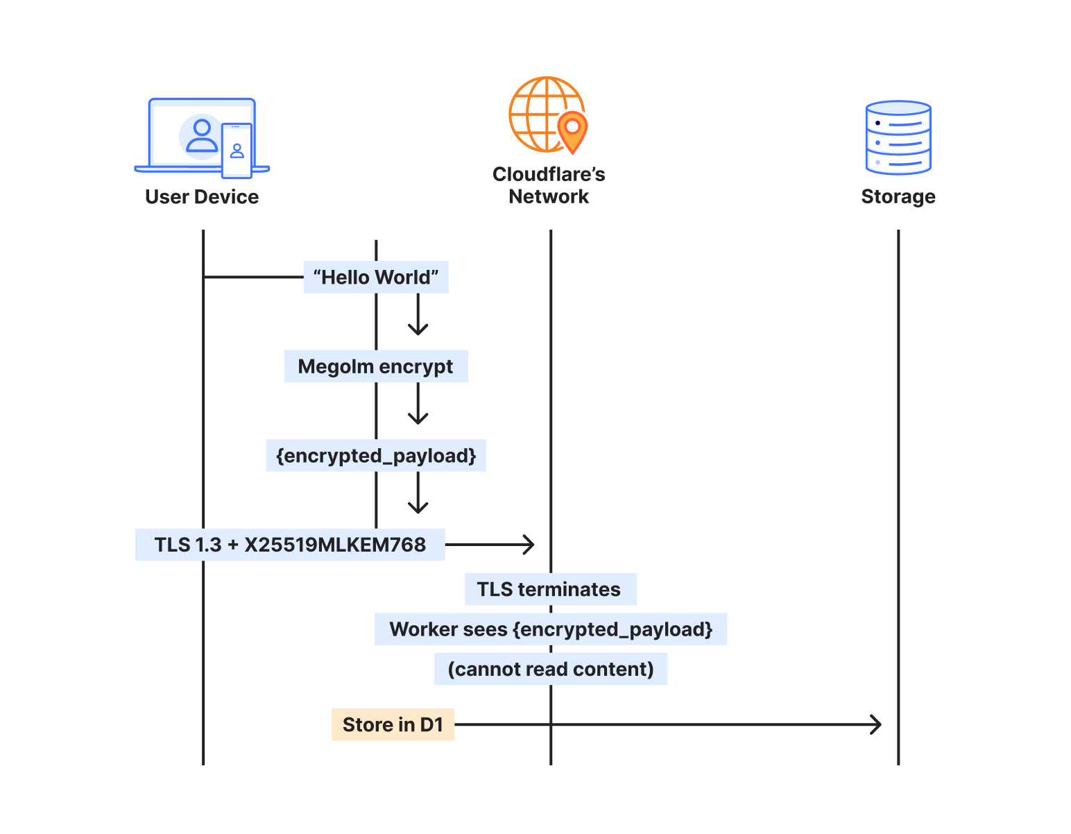
Understanding where encryption happens matters for security architecture. When someone sends a message through our homeserver, here’s the actual path:
The sender’s client takes the plaintext message and encrypts it with Megolm — Matrix’s end-to-end encryption. This encrypted payload then gets wrapped in TLS for transport. On Cloudflare, that TLS connection uses X25519MLKEM768, making it quantum-resistant.
The Worker terminates TLS, but what it receives is still encrypted — the Megolm ciphertext. We store that ciphertext in D1, index it by room and timestamp, and deliver it to recipients. But we never see the plaintext. The message “Hello, world” exists only on the sender’s device and the recipient’s device.
When the recipient syncs, the process reverses. They receive the encrypted payload over another quantum-resistant TLS connection, then decrypt locally with their Megolm session keys.
Two layers, independent protection
This creates defense in depth through two encryption layers that operate independently:
The transport layer (TLS) protects data in transit. It’s encrypted at the client and decrypted at the Cloudflare edge. With X25519MLKEM768, this layer is now post-quantum.
The application layer (Megolm E2EE) protects message content. It’s encrypted on the sender’s device and decrypted only on recipient devices. This uses classical Curve25519 cryptography.
Here’s why this architecture matters: Even if Matrix E2EE is eventually broken by quantum computers, the message content was never transmitted in a quantum-vulnerable form. The TLS layer that carried the E2EE ciphertext was itself post-quantum secured.
The post-quantum TLS acts as a quantum-resistant envelope around everything, including the classical E2EE layer. This buys time for the Matrix protocol to migrate to post-quantum E2EE algorithms without leaving current communications vulnerable to harvest-now-decrypt-later attacks.
Who sees what
Any Matrix homeserver operator — whether running Synapse on a VPS or this implementation on Workers — can see metadata: which rooms exist, who’s in them, when messages were sent. This is inherent to operating the server. You’re the operator; you control the infrastructure.
What no one in the infrastructure chain can see: message content. The E2EE payload is encrypted on sender devices before it ever hits the network. Cloudflare terminates TLS and passes requests to your Worker, but both see only Megolm ciphertext. Media in encrypted rooms is encrypted client-side before upload. Private keys never leave user devices.
The server processes ciphertext, not conversations. That’s true whether you’re self-hosting on bare metal or running on Workers.
What traditional deployments would need
Achieving post-quantum TLS on a traditional Matrix deployment would require upgrading OpenSSL or BoringSSL to a version supporting ML-KEM, configuring cipher suite preferences correctly, testing client compatibility across all Matrix apps, monitoring for TLS negotiation failures, staying current as PQC standards evolve, and handling clients that don’t support PQC gracefully.
With Workers, it’s automatic. Chrome, Firefox, and Edge all support X25519MLKEM768. Mobile apps using platform TLS stacks inherit this support. The security posture improves as Cloudflare’s PQC deployment expands — no action required on our part.
The storage architecture that made it work
The key insight from porting Tuwunel was that different data needs different consistency guarantees. We use each Cloudflare primitive for what it does best.
D1 for the data model
D1 stores everything that needs to survive restarts and support queries: users, rooms, events, device keys. Over 25 tables covering the full Matrix data model.
CREATE TABLE events (
	event_id TEXT PRIMARY KEY,
	room_id TEXT NOT NULL,
	sender TEXT NOT NULL,
	event_type TEXT NOT NULL,
	state_key TEXT,
	content TEXT NOT NULL,
	origin_server_ts INTEGER NOT NULL,
	depth INTEGER NOT NULL
);
D1’s SQLite foundation meant we could port Tuwunel’s queries with minimal changes. Joins, indexes, and aggregations work as expected.
We learned one hard lesson: D1’s eventual consistency breaks foreign key constraints. A write to rooms might not be visible when a subsequent write to events checks the foreign key — different replicas, different views of the world. We removed all foreign keys and enforce referential integrity in application code.
KV for ephemeral state
OAuth authorization codes live for 10 minutes. Refresh tokens last for a session. None of this needs SQL — it needs fast key-value access with automatic expiration.
// Store OAuth code with 10-minute TTL
kv.put(&format!("oauth_code:{}", code), &token_data)?
	.expiration_ttl(600)
	.execute()
	.await?;
KV’s global distribution means OAuth flows work fast regardless of where users are located.
R2 for media
Matrix media maps directly to R2. Upload an image, get back a content-addressed URL. Egress is free, which matters for a protocol where clients frequently download the same avatars and images.
Durable Objects for atomicity
Some operations can’t tolerate eventual consistency. When a client claims a one-time encryption key, that key must be atomically removed. If two clients claim the same key, encrypted session establishment fails.
Durable Objects provide single-threaded, strongly consistent storage:
#[durable_object]
pub struct UserKeysObject {
	state: State,
	env: Env,
}

impl UserKeysObject {
	async fn claim_otk(&self, algorithm: &str) -> Result<Option<Key>> {
    	// Atomic within single DO - no race conditions possible
    	let mut keys: Vec<Key> = self.state.storage()
        	.get("one_time_keys")
        	.await
        	.ok()
        	.flatten()
        	.unwrap_or_default();

    	if let Some(idx) = keys.iter().position(|k| k.algorithm == algorithm) {
        	let key = keys.remove(idx);
        	self.state.storage().put("one_time_keys", &keys).await?;
        	return Ok(Some(key));
    	}
    	Ok(None)
	}
}
We use UserKeysObject for E2EE key management, RoomObject for real-time room events like typing indicators and read receipts, and UserSyncObject for to-device message queues. The rest flows through D1.
Complete E2EE, complete OAuth
End-to-end encryption is non-negotiable for secure communications. Our implementation supports the full Matrix E2EE stack: device keys, cross-signing keys, one-time keys, fallback keys, key backup, and dehydrated devices.
Modern Matrix clients use OAuth 2.0/OIDC instead of legacy password flows. We implemented a complete OAuth provider: dynamic client registration, PKCE authorization, RS256-signed JWT tokens, token refresh with rotation, and standard OIDC discovery endpoints.
Point Element or any Matrix client at the domain, and it discovers everything automatically.
Sliding Sync for mobile
Traditional Matrix sync transfers megabytes of data on initial connection — every room, every state event, recent timeline for each. This destroys mobile battery and data plans.
Sliding Sync lets clients request exactly what they need. Instead of downloading everything, clients get the 20 most recent rooms with minimal state. As users scroll, they request more ranges. The server tracks position and sends only deltas.
Combined with edge execution, mobile clients can connect and render their room list in under 500ms — even on slow networks.
The comparison
For a homeserver serving a small team:
Traditional (VPS)
Workers
Monthly cost (idle)
$20-50
<$1
Monthly cost (active)
$20-50
$3-10
Global latency
100-300ms
20-50ms
Time to deploy
Hours
Seconds
Maintenance
Weekly
None
DDoS protection
Additional cost
Included
Post-quantum TLS
Complex setup
Automatic
*Based on public rates and metrics published by DigitalOcean, AWS Lightsail, and Linode as of January 15, 2026.
The economics improve further at scale. Traditional deployments require capacity planning and over-provisioning. Workers scale automatically.
The future of decentralized protocols
When we started this project, the goal was simply to see if the pieces would fit. Could a protocol as complex and stateful as Matrix — designed for heavy iron and persistent file systems — actually run on an ephemeral, serverless edge?
The answer is yes, but the implication is bigger than just Matrix.
By mapping traditional stateful components to Cloudflare’s primitives — Postgres to D1, Redis to KV, mutexes to Durable Objects — we proved that complex applications don’t need complex infrastructure. We stripped away the operating system, the database management, and the network configuration, leaving only the application logic and the data itself.
This architecture shifts the paradigm for self-hosting. It turns “running a server” from a chore into a utility. You get the sovereignty of owning your data without the burden of owning the infrastructure.
Matrix on Workers runs in production today, handling real encrypted communications for our team. It is fast, it is cheap, and it is arguably one of the most secure ways to deploy a homeserver today.
Ready to build secure, real-time applications on Workers? Get started withCloudflare Workers and exploreDurable Objects for your own stateful edge applications. Join ourDiscord community to connect with other developers building at the edge.
The US Supreme Court is considering the constitutionality of geofence warrants.
The case centers on the trial of Okello Chatrie, a Virginia man who pleaded guilty to a 2019 robbery outside of Richmond and was sentenced to almost 12 years in prison for stealing $195,000 at gunpoint.
Police probing the crime found security camera footage showing a man on a cell phone near the credit union that was robbed and asked Google to produce anonymized location data near the robbery site so they could determine who committed the crime. They did so, providing police with subscriber data for three people, one of whom was Chatrie. Police then searched Chatrie’s home and allegedly surfaced a gun, almost $100,000 in cash and incriminating notes.
Chatrie’s appeal challenges the constitutionality of geofence warrants, arguing that they violate individuals’ Fourth Amendment rights protecting against unreasonable searches.
Traditionally, curriculum planning has often looked like a linear list: Topic A leads to Topic B, which leads to Topic C. However, as educators we know that learning rarely happens in such a simple, linear way. Concepts are regularly covered in different overlapping topics, and students can often take different routes to reach the same destination.
In today’s blog we’re exploring learning graphs, a helpful tool that you can use to plan your computer science curriculum. We’ll share how they can provide educators with a clear, structured way to visualise students’ non-linear progression in a subject.
Find practical tips on how you can use learning graphs to design your curriculum
Read a summary of the research behind them
What is a learning graph?
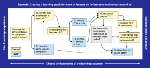
A learning graph is a visual tool for curriculum planning that moves beyond simple lists. At its core, a learning graph is a network of ‘nodes’ (specific concepts and skills) and ‘links’ (the connections between them).
Learning graphs build on research into ‘learning progressions’ and ‘knowledge maps’. They are a practical tool that educators can use to design and validate different curricula. For example, they can help teachers to:
Visualise and map progression
Identify curriculum gaps, so educators can shape and restructure learning experiences as necessary
Building a learning graph is an iterative process that helps you think critically about how different parts of your curriculum relate to each other.
Nodes and links
The first step in creating a learning graph is often to identify your start and end nodes. First, you consider the key concepts and skills that your learners must acquire by the end of a series of lessons. This gives you some end nodes to work towards. Then, you think about learners’ existing knowledge, to help determine your start point. You then work backwards and forwards between these points to identify the different nodes that learners need to cover to get from the beginning to the end.
Once you have determined your nodes, you add them to your graph and connect them via ‘links’ until your graph is complete. Where knowledge of particular concepts or skills is essential for learning others, you connect the nodes with solid lines. For prior learning that is helpful but not essential, you use dotted lines.
When developing a learning graph, there isn’t a specific level of granularity that you have to work towards. Progression can be as detailed or as high-level as you need. This makes them a helpful tool in creating bespoke learning experiences and curricula for learners.
Collaboration and development
It is most effective to design learning graphs collaboratively within a small group. This allows curriculum designers to discuss their ideas and challenge each other’s thinking, which helps hone the designs.
When creating learning graphs, it can be extremely useful to use a tool that is dynamic and allows you to move elements and make changes quickly and easily. At the Raspberry Pi Foundation, our team has experimented with a range of tools, including using editable shapes in Google Slides, collaborating in Figma, and arranging sticky notes on paper. We recommend finding a tool that works for you and the educators you are working with. Although it can work, we suggest avoiding using a pen and paper if possible, as designs can quickly become messy and difficult to navigate after lots of iterations.
The process of designing learning graphs has strong links to ABC learning design and the creation of concept maps, which can also be used for curriculum planning.
Learning graphs in your teaching
Once created, learning graphs can support you to design and adapt your curricula and assess your students’ learning.
For example, to help sequence learning, you can track or predict the paths through a topic most commonly taken by learners and use this to inform your curriculum design.
If you are adapting a unit of work for a specific qualification or new context, you can prune nodes that are not relevant and add any further knowledge and skills your learners need, then use the new learning graph to guide you as you develop the unit.
Finally, you can assess which node a learner has completed, and use this to identify the next logical step in their learning, ensuring the difficulty level is always appropriate.
Using learning graphs to support analysis
Another benefit of learning graphs is that they can be combined with lots of other frameworks, for example, Bloom’s taxonomy. This allows you to better assess and validate the learning journeys you have designed, and ensure that they are suitably accessible, challenging, and relevant for your learners.
There are a number of ways that you could link your learning graphs to other frameworks, such as annotating nodes with extra information, or using colour coding.
As well as working with learning graphs for specific learning experiences, you can connect multiple learning graphs together and analyse how they intersect. This can help identify inconsistencies between connected sequences of lessons. It can also help uncover broader themes of progression and highlight alternative learning pathways you might not have considered.
Find out more about learning graphs
If you’d like to find out more about learning graphs, you can download our Pedagogy Quick Read for free.
To find out more about how we use learning graphs when planning curriculum resources at the Raspberry Pi Foundation, take a look at our teaching and learning design principles.
2025-та вече е зад нас, а заедно с нея и цветът на годината, който, макар и наречен с изтънчено звучащото наименование Mocha Mousse („мока мус“), на вид по-скоро напомня оттичаща се в канализацията отпадъчна материя. С настъпването на новата година обаче сме поканени оптимистично да обърнем взор нагоре към небето (и да заровим глави в речниците).
За цвят на 2026-та Pantone Color Institute обяви т.нар. Cloud Dancer, чието наименование българските медии превеждат като „облачно бяло“,
въпреки че думата „бяло“ очевидно отсъства в „оригинала“ и по-точният му превод е нещо като „танцьор в облаците“. Описан като мек, неутрален, въздушен нюанс (който на български би могъл да се определи и със злощастното название „мръснобяло“), според Pantone идеята е цветът да символизира спокойствие, простота, яснота, релаксация и както подобава на всеки старт на годината – ново начало.
Горното описание, обобщено от многобройните медийни съобщения по темата, демонстрира удивителната способност на компанията да приписва на цветовете характеристики, които не са им естествено присъщи непременно. Освен чрез засуканите наименования Pantone постига това и с високопарните описания, които придружават анонсирането на всеки цвят и с всяка изминала година все повече наподобяват – както личи от най-новия избор – въздух под налягане.
Така например лаици като мен и вас биха помислили, че през последните 26 години, откакто датира традицията, оранжевото (макар и в различни нюанси) е било цвят на годината цели четири пъти. Да, ама не: според Pantone цветът на 2004 г. е Tigerlily („тигров лилиум“) – „ярък, смел, страстен и подмладяващ“; на 2012 г. той е Tangerine Tango („мандаринено танго“) – „магнетичен оттенък, който напомня за сияйните нюанси на залеза и излъчва топлина и енергия“; на 2019 г. е Living Coral („жив корал“) – „оживяващ и жизнеутвърждаващ коралов оттенък със златист подтон, който енергизира и съживява“; а на 2024 г. е Peach Fuzz („прасковен мъх“) – „топъл и уютен оттенък между розово и оранжево с винтидж атмосфера, който носи усещане за нова модерност и нежност, както и послание за грижа и споделяне, общност и сътрудничество“.
Подобна е ситуацията и със сините, розовите и зелените разцветки, разновидности на които неколкократно са избирани за цвят на годината. Бялото, в какъвто и да било нюанс, оглавява класацията за първи път. Като за цвят, който в същността си представлява липса на цветове, изборът на Pantone за 2026 г. предизвиква множество критики – те варират от твърдения, че бялото е скучно и безлично, до обвинения в „далтонизъм“¹ по отношение на съвсем небезобидните обществени трусове, геополитически проблеми и икономически предизвикателства, с които в момента се сблъсква светът.
В това отношение
цветовете са като думите – те притежават нюанси, предизвикват лични асоциации и носят разнообразни конотации според контекста,
които не могат да бъдат изцяло наложени отвън. Това важи с особена сила за белия цвят, който всъщност съдържа в себе си всички останали цветове. Подобно на табула раза, върху него може да се проектират всякакви, често противоположни смисли и значения. Защото бялото – освен невинност (в булчинската рокля), чистота и духовност (в одеждите на дъновистите или на папата) или ново началото (на белия лист) – също така би могло да символизира траур (в източните традиции), капитулация (в бялото знаме), расизъм и вяра в превъзходството на белите (в мантиите на Ку-клукс-клан).
По сходен начин думата „облак“ също съдържа „цял спектър“ от възможни значения и конотации. Освен приписаните му от Pantone лекота, ефирност и мекота, облакът може да означава и много други, не непременно възвишени неща: непостоянство и разсеяност, замъгленост и неяснота, мрачно предзнаменование и заплаха. Както и място за съхранение на дигитални данни. Или пък мента с мастика.
Ако пък въпросният облак, освен бял, е и в умалителна форма, много българи със сигурност биха го свързали с носталгия по родината.
Лично аз винаги се сещам за трогателното, каращо ме да настръхна изпълнение на „Облаче ле бяло“ на Силви Вартан.
В този текст ще се опитам да отговоря на въпроса, с който започва песента – „Я кажи ми, облаче ле бяло, /отде идеш, де си ми летяло?“, – но от етимологична гледна точка. Освен коренно различните разбирания за това какво представляват облаците, проследяването на произхода на думата през различни древни или праезици, а оттам и до техните съвременни наследници разкрива доста любопитни семантични взаимовръзки както между езиците, така и вътре в самите тях. Макар и заобиколно, част от нишките водят и до българския.
В романските езици думите за „облак“ – nuage на френски, nuvola на италиански, nube на испански, nor на румънски – неизненадващо, произлизат от латинския. Изненадващото в случая е, че същият латински корен – nubes („облак“) – е в основата и на дума, която през френския е навлязла и в българския, а в този текст е особено актуална и се появява многократно: това е думата „нюанс“.
Въпреки сходното произношение и семантика латинската дума nubes, която произлиза от праиндоевропейския глагол *(s)newdʰ- („покривам“), не споделя родство с латинското название nebula („мъгла“)² – то произлиза от праиндоевропейската дума *nébʰos („облак“). Именно тя стои и в основата на славянските вариации на думата „небе“.
От същия праиндоевропейски корен произлизат и двете думи за „облак“, които се срещат както в древния, така и в съвременния гръцки език– νέφος(néfos) и νεφέλη(neféli). Сходното звучене, както и концептуално близките значения тук също могат да ни подведат, че от тези понятия произлиза чудесната дума „нефелен“. Българският етимологичният речник обаче опровергава тези очаквания, като проследява произхода ѝ до прилагателното ανωφελής(anofelís), което има друг корен и означава „безполезен“.
Думата „облак“ в българския и в останалите славянски езици има праславянски корени – *obolkъ, от представката *оb– („около“) + *volk- („тегля, влача“), – като по този начин споделя сходна етимология с глагола „обличам“.³
Макар, че названието присъства с малки вариации във всички славянски езици, някои от тях разполагат с допълнителни думи, с които обозначават струпаните водни пари в атмосферата. Чешкият например прави разлика между белия, незаплашителен oblak и тъмния, буреносен mrak. На полски думата obłok се смята за по-поетична и „възвишена“, докато всекидневната дума е chmura. „Хмара“ означава „облак“ и на украински. Макар да не присъства нито в моя личен речник, нито в тълковния речник на БАН, според bgjargon.com тази дума съществува и в българския език със следната дефиниция: „гъста пушилка, думан, сумрак; нещо непрогледно и мрачно“.
Произходът на днешната английска дума за „облак“ също е доста далечен – както концептуално, така и пространствено – от ефирния cloud в наименованието на Pantone: първоначалното значение на староанглийската дума clud е ‘скала, камък, буца пръст, маса’ и няма нищо общо с небето. С развитието на езика обаче значението ѝ се разширява и става метафорично, докато към края на XV век, с преминаването към ранния модерен английски, идеята за земната маса отпада изцяло и се заменя с концепцията за небесната⁴.
Съвременната английска дума sky, тоест „небе“, претърпява паралелна трансформация. Наследена от староскандинавски, първоначално тя навлиза със значението „облак“, което в (почти) всички скандинавски езици се запазва и до днес⁵. С течение на времето обаче смисълът ѝ се променя и тя постепенно измества напълно двете староанглийски думи за „небе“: heofon, откъдето идва съвременната дума heaven („рай“), и weolcan („облак, небе“), която произлиза от прагерманската *wulkną, откъдето пък идва съвременната немска дума за „облак“ – Wolke. (И тук, съвсем ненадейно, откриваме връзка с българския през общия праиндоевропейски корен *wl̥g-nó-s, откъдето произлиза праславянската дума *volga, като реката, а оттам и съвременната „влага“.)
Както личи от горните примери, понятията за „облак“ и „небе“ често са свързани, а нерядко се и припокриват. Чешкият предоставя интересен пример за това – освен двете думи за „облак“, споменати по-горе, в него има и две отделни названия за „небе“: nebe – с по-абстрактно значение, и obloha, което се използва в буквален смисъл. Ето как „В небето има облаци“ на чешки би могло да изглежда така: Na obloze jsou oblaky. Или пък така: Na nebi jsou mraky.
Особено забавни в това отношение са и калките на американската дума skyscraper в различните езици. Някои от тях остават верни на оригинала, като двете съставни части се превеждат буквално, например българският „небостъргач“, сръбският „небодер“, литовският dangoraižis, турският gökdelen и гръцкият ουρανοξύστης (ouranoxýstis), макар и понякога местата на корените да се разменят, като във френския gratte-ciel, испанския rascacielos и румънския zgârie-nori. В други езици се прилага по-свободен подход и думата „небе“ се заменя с „облак“, например в немския Wolkenkratzer, унгарския felhőkarcoló, финландския pilvenpiirtäjä, както и в личните ми фаворити – украинския „хмарочос“, чешкия mrakodrap и македонския „облакодер“. Положението става съвсем хаотично в скандинавските езици (skyskraper на норвежки, skyskraber на датски и skýjakljúfur на исландски), които хем уж запазват англоезичното „небе“, хем всъщност разчитат на оригиналното значение на думата като „облак“. На шведски названието е skyskrapa, обаче там случаят е специален, тъй като sky (произнася се като „хуѝ“) се използва рядко, но има идентично значение с думата в английския.
За концептуалната и семантична взаимосвързаност (нерядко до степен на взаимозаменяемост) между облаците и небето свидетелства и изразът „седмото небе“ и итерациите му на различни езици. Облаците присъстват в еквивалентните изрази на английски – to be on cloud nine, на немски – auf Wolke sieben sein, на френски – être sur un petit nuage, докато в българския и в много други езици от различни семейства изразът за върховно щастие препраща към небето, и то конкретно към седмото: být v sedmém nebi (чешки), essere al settimo cielo (италиански), vara i sjunde himlen (шведски), في السماء السابعة (арабски), בַּשָּׁמַיִם הַשְּׁבִיעִים (иврит).
От горните примери се вижда, че докато повечето езици използват числото седем (без значение дали във връзка с облак, или с небе), в английския облакът на блаженството е заведен под номер девет (макар че и там съществува вече остарелият и далеч не толкова популярен идиом seventh heaven).
Седмѝцата може да се обясни с древната символика и значение на числото в християнската, ислямската и еврейската традиция. За разлика от това число, деветката в английския израз има много по-нов и не съвсем ясен произход. Според широко разпространената теория тя е заимствана от Международния атлас на облаците, първоначално издаден през 1896 г., където са описани десет вида облаци – деветият от тях е т.нар. cumulonimbus, който се издига най-високо в атмосферата и изглежда най-голям, пухкав и комфортен. Изборът на точно този вид облак като синоним за блаженство обаче е озадачаващ, като се вземе предвид, че наименованието му означава „купесто-дъждовен“ и че точно той поражда мълнии, гръмотевични бури, проливни дъждове, смерчове и други опасни метеорологични условия.
Тепърва предстои да видим
дали тази година ще танцуваме на деветия облак, на облак номер 11-4201 TCX (както е обозначен Cloud Dancer на Pantone),или в деветия кръг на ада.
Едно обаче е сигурно: годината несъмнено ще е облачна. Но нека бъдем оптимисти и да се надяваме, че английската поговорка every cloud has a silver lining, която произлиза от творба на Джон Милтън и буквално означава, че всеки облак има сребърен хастар, ще се окаже вярна – тоест че всяко зло наистина ще е за добро. Все пак дори Дантевият „Ад“ завършва с надеждата, че след преминаването през деветия кръг отново ще видим звездите.
1 Терминът „далтонизъм“, вероятно навлязъл в българския език от френския, произлиза от името на английския химик Джон Далтон, който сам е страдал от това зрително нарушение и първи го е описал. Подобно на наименованията на облаците, които съществуват в разговорна и в латинска форма, зрителният дефект, водещ до неспособността да се разграничават определени цветове, има още две наименования: „цветна слепота“ и „дисхроматопсия“.
2 От латинската дума nebula произлиза и английското прилагателно nebulous, което най-често се използва преносно и означава ‘неясен, мъгляв, неопределен’. Макар че то не е навлязло в говоримия български език, астрономите използват термина „небуларен“, който се отнася за космическите мъглявини.
3 Освен „облак“, от същия праславянски корен – *volk- (‘тегля, влача’) – произлиза и думата „влак“. Праиндоевропейският му родител *welk- пък е в основата на английския глагол walk (‘ходя’). Сходна идея присъства и в думата за „облак“ на арабски (سحاب/saḥāb), която произлиза от корен, означаващ ‘издърпване, влачене’.
4 Въпреки трансформацията в значението на думата clud, в съвременния английския се срещат редица думи, чието значение е свързано с оригиналното значение на думата (‘скала, камък, буца пръст, маса’), като например clod и clump (и двете със значение ‘буца’), clot (‘съсирек’) и cluster (‘струпване’).
5Sky означава „облак“ на всички скандинавски езици с изключение на шведския, където думата, макар че се смята за остаряла, се възприема по-скоро с англоезичното значение на „небе“, докато съвременната дума за „облак“ е moln. Тя, за съжаление, не е етимологично свързана с българската „мълния“, но нейният праславянски предшественик (*mъldni) все пак споделя праиндоевропейски корен (*meldʰ-) с друго скандинавско наименование, а именно Mjǫllnir – магическия чук на Тор, нордическия бог на гръмотевиците, светкавиците и бурите.
В рубриката „От дума на дума“ Екатерина Петрова търси актуални, интересни или новопоявили се думи от нашето ежедневие и проследява често изненадващия им произход, развитието на значенията им във времето и взаимовръзките им с близки и далечни езици.
When you enable IAM Identity center, it provides an access portal for workforce users to access their AWS applications and accounts either by signing in to the access portal using a URL or by using a bookmark for the application URL. In either case, the access portal handles user authentication before granting access to applications and accounts. Supporting both IPv4 and IPv6 connectivity to the access portal helps facilitate seamless access for clients, such as browsers and applications, regardless of their network configuration.
The launch of IPv6 support in IAM Identity Center introduces new dual-stack endpoints that support both IPv4 and IPv6, so that users can connect using IPv4, IPv6, or dual-stack clients. Current IPv4 endpoints continue to function with no action required. The dual stack capability offered by Identity Center extends to managed applications. When users access the application dual-stack endpoint, the application automatically routes to the Identity Center dual-stack endpoint for authentication. To use Identity Center from IPv6 clients, you must direct your workforce to use the new dual-stack endpoints, and update configurations on your external identity provider (IdP), if you use one.
In this post, we show you how to update your configuration to allow IPv6 clients to connect directly to IAM Identity Center endpoints without requiring network address translation services. We also show you how to monitor which endpoint users are connecting to. Before diving into the implementation details, let’s review the key phases of the transition process.
Transition overview
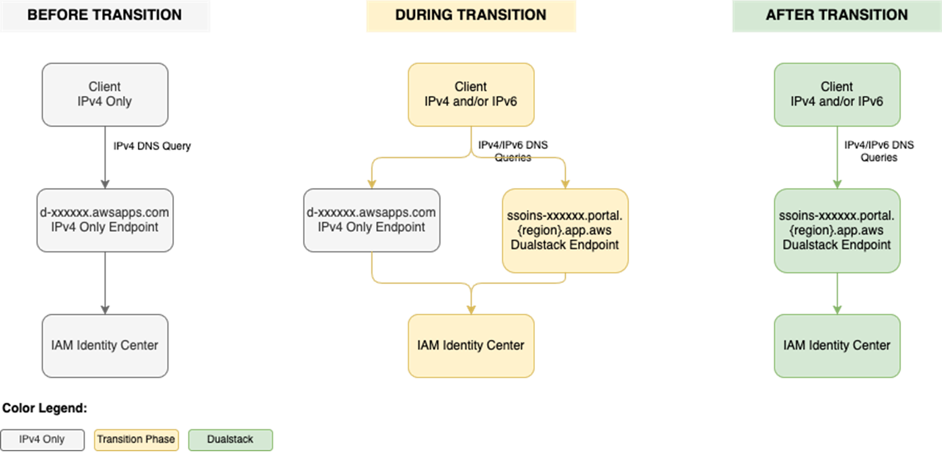
To use IAM Identity Center from an IPv6 network and client, you need to use the new dual-stack endpoints. Figure 1 shows what the transition from IPv4 to IPv6 over dual-stack endpoints looks like when using Identity Center. The figure shows:
A before state where clients use the IPv4 endpoints.
The transition phase, when your clients use a combination of IPv4 and dual-stack endpoints.
After the transition is complete, your clients will connect to dual-stack endpoints using their IPv4 or IPv6, depending on their preferences.
Figure 1: Transition from IPv4-only to dual-stack endpoints
Prerequisites
You must have the following prerequisites in place to enable IPv6 access for your workforce users and administrators:
Work with your network administrators to update the configuration of your firewalls and gateways and to verify that your clients, such as laptops or desktops, are ready to accept IPv6 connectivity. If you have already enabled IPv6 connectivity for other AWS services, you might be familiar with these changes. Next, implement the two steps that follow.
Step 1: Update your IdP configuration
You can skip this step If you don’t use an external IdP as your identity source.
In this step, you update the Assertion Consumer Service (ACS) URL from your IAM Identity Center instance into your IdP’s configuration for single sign-on and the SCIM configuration for user provisioning. Your IdP’s capability determines how you update the ACS URLs. If your IdP supports multiple ACS URLs, configure both IPv4 and dual-stack URLs to enable a flexible transition. With that configuration, some users can continue using IPv4-only endpoints while others use dual-stack endpoints for IPv6. If your IdP supports only one ACS URL, to use IPv6 you must update the new dual-stack ACS URL in your IdP and transition all users to using dual-stack endpoints. If you don’t use an external IdP, you can skip this step and go to the next step.
Update both the SAML single sign-on and the SCIM provisioning configurations:
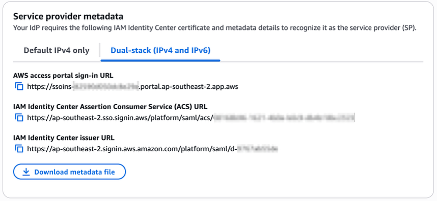
Update the single sign-on settings in your IdP to use the new dual-stack URLs. First, locate the URLs in the AWS Management Console for IAM Identity Center.
Choose Settings in the navigation pane and then select Identity source.
Choose Actions and select Manage authentication.
in Under Manage SAML 2.0 authentication, you will find the following URLs under Service provider metadata:
AWS access portal sign-in URL
IAM Identity Center Assertion Consumer Service (ACS) URL
IAM Identity Center issuer URL
If your IdP supports multiple ACS URLs, then add the dual-stack URL to your IdP configuration alongside existing IPv4 one. With this setting, you and your users can decide when to start using the dual-stack endpoints, without all users in your organization having to switch together.
Figure 2: Dual-stack single sign-on URLs
If your IdP does not support multiple ACS URLs, replace the existing IPv4 URL with the new dual-stack URL, and switch your workforce to use only the dual-stack endpoints.
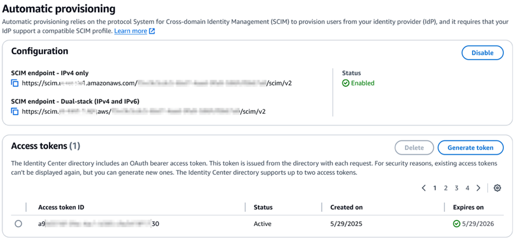
Update the provisioning endpoint in your IdP. Choose Settings in the navigation pane and under Identity source, choose Actions and select Manage provisioning. Under Automatic provisioning, copy the new SCIM endpoint that ends in api.aws. Update this new URL in your external IdP.
Figure 3: Dual-stack SCIM endpoint URL
Step 2: Locate and share the new dual-stack endpoints
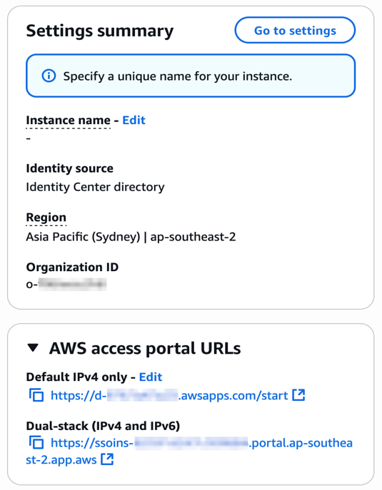
Your organization needs two kinds of URLs for IPv6 connectivity. The first is the new dual-stack access portal URL that your workforce users use to access their assigned AWS applications and accounts. The dual-stack access portal URL is available in the IAM Identity Center console, listed as the Dual-stack in the Settings summary (you might need to expand the Access portal URLs section, shown in Figure 4).
This dual-stack URL ends with app.aws as its top-level domain (TLD). Share this URL with your workforce and ask them to use this dual-stack URL to connect over IPv6. As an example, if your workforce uses the access portal to access AWS accounts, they will need to sign in through the new dual-stack access portal URL when using IPv6 connectivity. Alternately, if your workforce accesses the application URL, you need to enable the dual-stack application URL following application-specific instructions. For more information, see AWS services that support IPv6.
The URLs that administrators use to manage IAM Identity Center are the second kind of URL your organization needs. The new dual-stack service endpoints end in api.aws as their TLD and are listed in the Identity Center service endpoints. Administrators can use these service endpoints to manage users and groups in Identity Center, update their access to applications and resources, and perform other management operations. As an example, if your administrator uses identitystore.{region}.amazonaws.com to manage users and groups in Identity Center, they should now use the dual-stack version of the same service endpoint which is identitystore.{region}.api.aws, so they can connect to service endpoints using IPv6 clients and networks.
If your users or administrators use an AWS SDK to access AWS applications and accounts or manage services, follow Dual-stack and FIPS endpoints to enable connectivity to the dual-stack endpoints.
After completing these two steps, your workforce and administrators can connect to IAM Identity Center using IPv6. Remember, these endpoints also support IPv4, so clients not yet IPv6-capable can continue to connect using IPv4.
Monitoring dual-stack endpoint usage
You can optionally monitor AWS CloudTrail logs to track usage of dual-stack endpoints. The key difference between IPv4-only and dual-stack endpoint usage is the TLD and appears in the clientProvidedHostHeader field. The following example shows the difference between these CloudTrail events for the CreateTokenWithIAM API call.
IAM Identity Center now allows clients to connect over IPv6 natively with no network address translation infrastructure. This post showed you how to transition your organization to use IPv6 with Identity Center and its integrated applications. Remember that existing IPv4 endpoints will continue to function, so you can transition at your own pace. Also, no immediate action is required by you. However, we recommend planning your transition to take advantage of IPv6 benefits and meet compliance requirements. If you have questions, comments, or concerns, contact AWS Support, or start a new thread in the IAM Identity Center re:Post channel.
If you have feedback about this post, submit comments in the Comments section below. If you have questions about this post, contact AWS Support.
Our previous blog posts (part 1, part 2, part 3) detailed how Netflix’s Graph Search platform addresses the challenges of searching across federated data sets within Netflix’s enterprise ecosystem. Although highly scalable and easy to configure, it still relies on a structured query language for input. Natural language based search has been possible for some time, but the level of effort required was high. The emergence of readily-available AI, specifically Large Language Models (LLMs), has created new opportunities to integrate AI search features, with a smaller investment and improved accuracy.
While Text-to-Query and Text-to-SQL are established problems, the complexity of distributed Graph Search data in the GraphQL ecosystem necessitates innovative solutions. This is the first in a three-part series where we will detail our journey: how we implemented these solutions, evaluated their performance, and ultimately evolved them into a self-managed platform.
The Need for Intuitive Search: Addressing Business and Product Demands
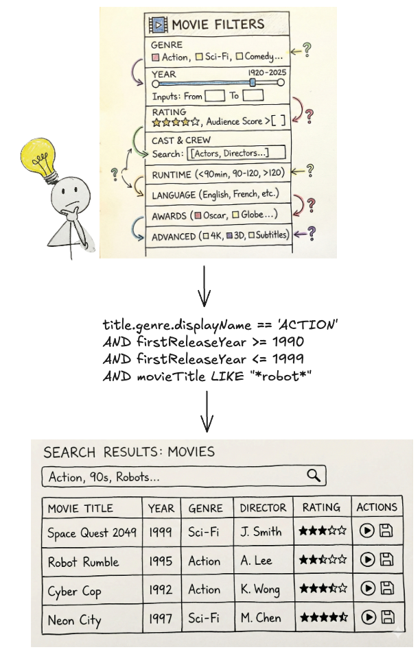
Natural language search is the ability to use everyday language to retrieve information as opposed to complex, structured query languages like the Graph Search Filter Domain Specific Language (DSL). When users interact with 100’s of various UIs within the suite of Content and Business Products applications, a frequent task is filtering a data table like the one below:
Example Content and Business Products application view
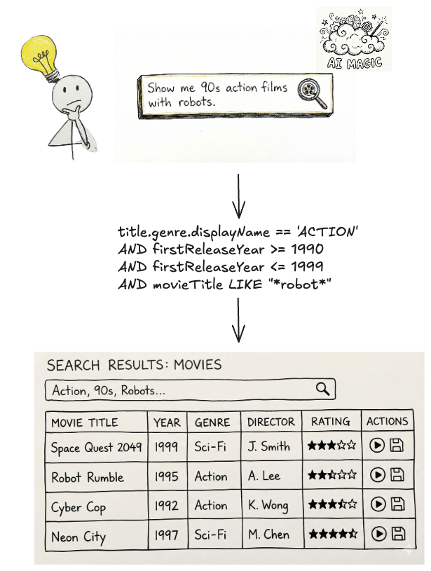
Ideally, a user simply wants to satisfy a query like “I want to see all movies from the 90s about robots from the US.” Because the underlying platform operates on the Graph Search Filter DSL, the application acts as an intermediary. Users input their requirements through UI elements — toggling facets or using query builders — and the system programmatically converts these interactions into a valid DSL query to filter the data.
The Complexity of filtering and DSL generation
This process presents a few issues.
Today, many applications have bespoke components for collecting user input — the experience varies across them and they have inconsistent support for the DSL. Users need to “learn” how to use each application to achieve their goals.
Additionally, some domains have hundreds of fields in an index that could be faceted or filtered by. A subject matter expert (SME) may know exactly what they want to accomplish, but be bottlenecked by the inefficient pace of filling out a large scale UI form and translating their questions in order to encode it in a representation Graph Search needs.
Most importantly, users think and operate using natural language, not technical constructs like query builders, components, or DSLs. By requiring them to switch contexts, we introduce friction that slows them down or even prevents their progress.
With readily-available AI components, our users can now interact with our systems through natural language. The challenge now is to make sure our offering, searching Netflix’s complex enterprise state with natural language, is an intuitive and trustworthy experience.
Natural language queries translated into Graph Search Filter DSL
We’ve made a decision to pursue generating Graph Search Filter statements from natural language to meet this need. Our intention is to augment and not replace existing applications with retrieval augmented generation (RAG), providing tooling and capabilities so that applications in our ecosystem have newly accessible means of processing and presenting their data in their distinct domain flavours. It should be noted that all the work here has direct application to building a RAG system on top of Graph Search in the future.
Under the Hood: Our Approach to Text-to-Query
The core function of the text-to-query process is converting a user’s (often ambiguous) natural language question into a structured query. We primarily achieve this through the use of an LLM.
Before we dive deeper, let’s quickly revisit the structure of Graph Search Filter DSL. Each Graph Search index is defined by a GraphQL query, made up of a collection of fields. Each field has a type e.g. boolean, string, and some have their permitted values governed by controlled vocabularies — a standardized and governed list of values (like an enumeration, or a foreign key). The names of those fields can be used to construct expressions using comparison (e.g. > or ==) or inclusion/exclusion operators (e.g. IN). In turn those expressions can be combined using logical operators (e.g. AND) to construct complex statements.
Graph Search Filter DSL
With that understanding, we can now more rigorously define the conversion process. We need the LLM to generate a Graph Search Filter DSL statement that is syntactically, semantically, and pragmatically correct.
Syntactic correctness is easy — does it parse? To be syntactically correct, the generated statement must be well formedi.e. follow the grammar of the Graph Search Filter DSL.
Semantic correctness adds some additional complexity as it requires more knowledge of the index itself. To be semantically correct:
it must respect the field types i.e. only use comparisons that make sense given the underlying type;
it must only use fields that are actually present in the index, i.e. does not hallucinate;
when the values of a field are constrained to a controlled vocabulary, any comparison must only use values from that controlled vocabulary.
Pragmatic correctness is much more difficult. It asks the question: does the generated filter actually capture the intent of the user’s query?
The following sections will detail how we pre-process the user’s question to create appropriate context for the instructions that we will provide to the LLM — both of which are fundamental to LLM interaction — as well as post-processing we perform on the generated statement to validate it, and help users understand and trust the results they receive.
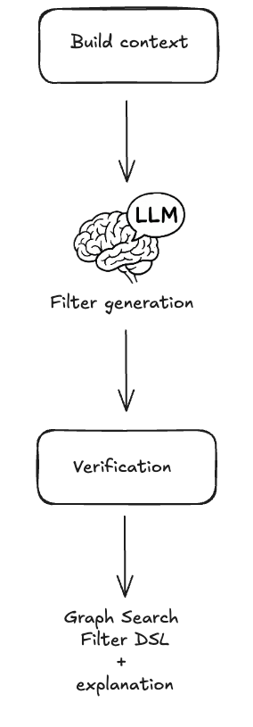
At a high level that process looks like this:
Graph Search FIlter DSL generation process
Context Engineering
Preparation for the filter generation task is predominantly engineering the appropriate context. The LLM will need access to the fields of an index and their metadata in order to construct semantically correct filters. As the indices are defined by GraphQL queries, we can use the type information from the GraphQL schema to derive much of the required information. For some fields, there is additional information we can provide beyond what’s available in the schema as well, in particular permissible values that pull from controlled vocabularies.
Each field in the index is associated with metadata as seen below, and that metadata is provided as part of the context.
Graph Search index representation
The field is derived from the document path as characterized by the GraphQL query.
The description is the comment from the GraphQL schema for the field.
The type is derived from the GraphQL schema for the field e.g. Boolean, String, enum. We also support an additional controlled vocabulary type we will discuss more of shortly.
The valid values are derived from enum values for the enum type or from a controlled vocabulary as we will now discuss.
A controlled vocabulary is a specific field type that consists of a finite set of allowed values, which are defined by a SMEs or domain owners. Index fields can be associated with a particular controlled vocabulary, e.g. countries with members such as Spain and Thailand, and any usage of that field within a generated statement must refer to values from that vocabulary.
Naively providing all the metadata as context to the LLM worked for simple cases but did not scale. Some indices have hundreds of fields and some controlled vocabularies have thousands of valid values. Providing all of those, especially the controlled vocabulary values and their accompanying metadata, expands the context; this proportionally increases latency and decreases the correctness of generated filter statements. Not providing the values wasn’t an option as we needed to ground the LLMs generated statements- without them, the LLM would frequently hallucinate values that did not exist.
Curating the context to an appropriate subset was a problem we addressed using the well known RAG pattern.
Field RAG
As mentioned previously, some indices have hundreds of fields, however, most user’s questions typically refer only to a handful of them. If there was no cost in including them all, we would, but as mentioned prior, there is a cost in terms of the latency of query generation as well as the correctness of the generated query (e.g. needle-in-the-hackstack problem) and non-deterministic results.
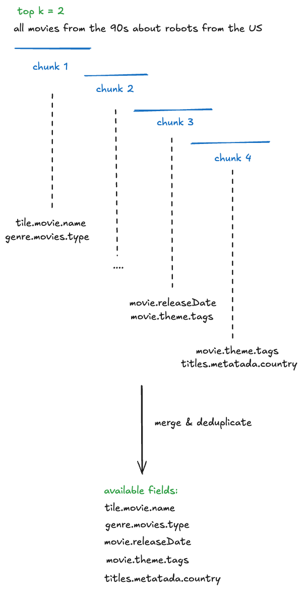
To determine which subset of fields to include in the context, we “match” them against the intent of the user’s question.
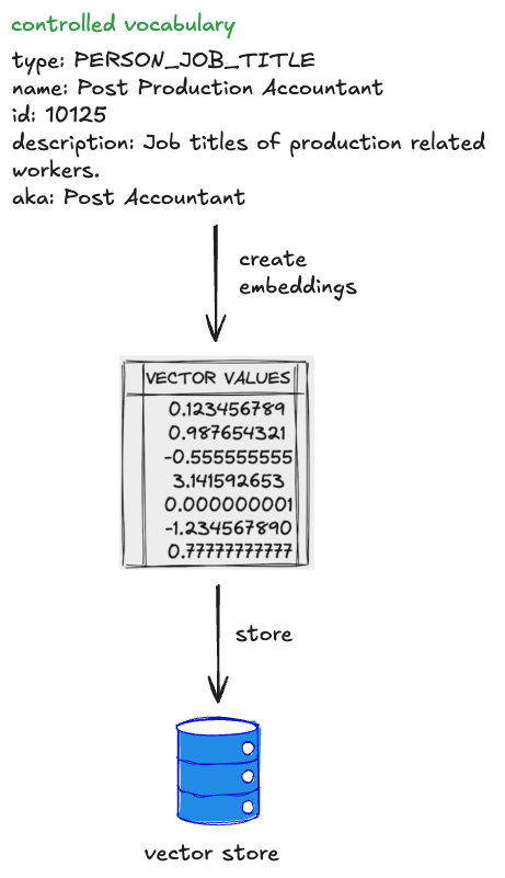
Embeddings are created for index fields and their metadata (name, description, type) and are indexed in a vector store
At filter generation time, the user’s question is chunked with an overlapping strategy. For each chunk, we perform a vector search to identify the top K most relevant values and the fields to which they belong.
Deduplication: The top K fields from each chunk are both consolidated and deduplicated before being provided as context to the system instructions.
Field RAG process (chunking, merge, deduplicate)
Controlled Vocabularies RAG
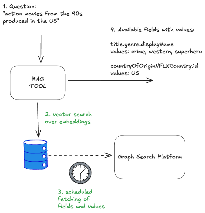
Index fields of the controlled vocabulary type are associated with a particular controlled vocabulary, again, countries are one example. Given a user’s question, we can infer whether or not it refers to values of a particular controlled vocabulary. In turn, by knowing which controlled vocabulary values are present, we can identify additional, related index fields that should be included in the context that may not have been identified by the field RAG step.
Each controlled vocabulary value has:
a unique identifier within its type;
a human readable display name;
a description of the value;
also-known-as values or AKA display names, e.g. “romcom” for “Romantic Comedy”.
To determine which subset of values to include in the context for controlled vocabulary fields (and also possibly infer additional fields), we “match” them against the user’s question.
Embeddings are created for controlled vocabulary values and their metadata, and these are indexed in a vector store. The controlled vocabularies are available via GraphQL and are regularly fetched and reindexed so this system stays up to date with any changes in the domain.
At filter generation time, the user’s question is chunked. For each chunk, we perform a vector search to identify the top K most relevant values (but only for the controlled vocabularies that are associated with fields in the index)
The top K values from each chunk are deduplicated by their controlled vocabulary type. The associated field definition is then injected into the context along with the matched values.
Controlled Vocabularies RAG
Combining both approaches, the RAG of fields and controlled vocabularies, we end up with the solution that each input question resolves in available and matched fields and values:
Field and CV RAG
The quality of results generated by the RAG tool can be significantly enhanced by tuning its various parameters, or “levers.” These include strategies for reranking, chunking, and the selection of different embedding generation models. The careful and systematic evaluation of these factors will be the focus of the subsequent parts of this series.
The Instructions
Once the context is constructed, it is provided to the LLM with a set of instructions and the user’s question. The instructions can be summarised as follows: “Given a natural language question, generate a syntactically, semantically, and pragmatically correct filter statement given the availability of the following index fields and their metadata.”
In order to generate a syntactically correct filter statement, the instructions include the syntax rules of the DSL.
In order to generate a semantically correct filter statement, the instructions tell the LLM to ground the generated statement in the provided context.
In order to generate a pragmatically correct filter statement, so far we focus on better context engineering to ensure that only the most relevant fields and values are provided. We haven’t identified any instructions that make the LLM just “do better” at this aspect of the task.
Graph Search Filter DSL generation
After the filter statement is generated by the LLM, we deterministically validate it prior to returning the values to the user.
Validation
Syntactic Correctness
Syntactic correctness ensures the LLM output is a parsable filter statement. We utilize an Abstract Syntax Tree (AST) parser built for our custom DSL. If the generated string fails to parse into a valid AST, we know immediately that the query is malformed and there is a fundamental issue with the generation.
The other approach to solve this problem could be using the structured outputs modes provided by some LLMs. However, our initial evaluation yielded mixed results, as the custom DSL is not natively supported and requires further work.
Semantic Correctness
Despite careful context engineering using the RAG pattern, the LLM sometimes hallucinates both fields and available values in the generated filter statement. The most straightforward way of preventing this phenomenon is validating the generated filters against available index metadata. This approach does not impact the overall latency of the system, as we are already working with an AST of the filter statement, and the metadata is freely available from the context engineering stage.
DSL verification & hallucinations
If a hallucination is detected it can be returned as an error to a user, indicating the need to refine the query, or can be provided back to the LLM in the form of a feedback loop for self correction.
This increases the filter generation time, so should be used cautiously with a limited number of retries.
Building Confidence
You probably noticed we are not validating the generated filter for pragmatic correctness. That task is the hardest challenge: The filter parses (syntactic) and uses real fields (semantic), but is it what the user meant? When a user searches for “Dark”, do they mean the specific German sci-fi series Dark, or are they browsing for the mood category “dark TV shows”?
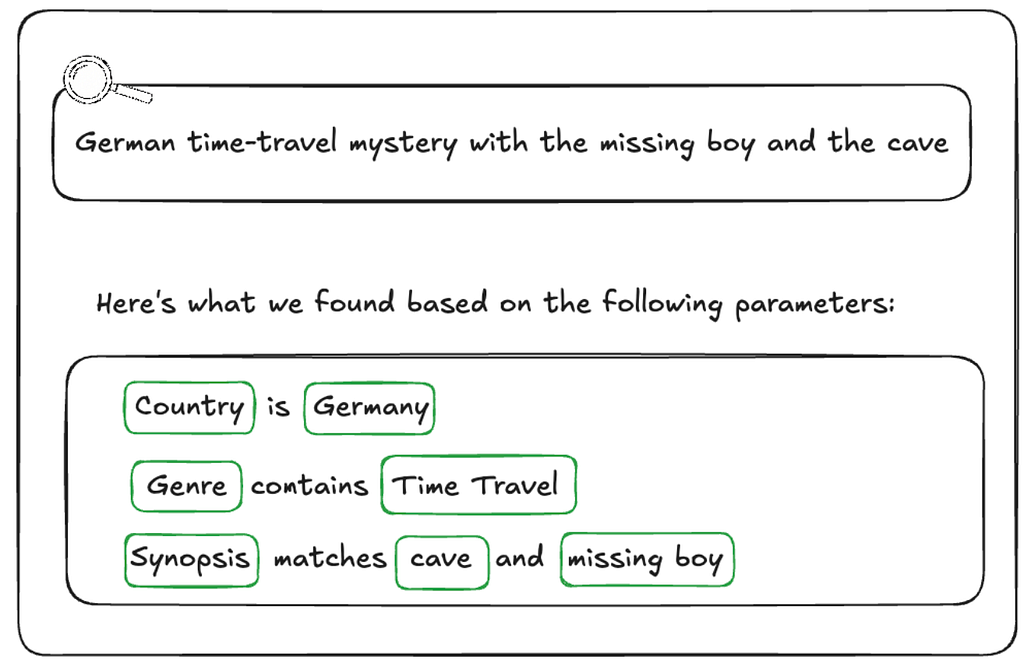
The gap between what a user intended and the generated filter statement is often caused by ambiguity. Ambiguity stems from the compression of natural language. A user says “German time-travel mystery with the missing boy and the cave” but the index contains discrete metadata fields like releaseYear, genreTags, and synopsisKeywords.
How do we ensure users aren’t inadvertently led to wrong answers or to answers for questions they didn’t ask?
Showing Our Work
One way we are handling ambiguity is by showing our work. We visualise the generated filters in the UI in a user-friendly way allowing them to very clearly see if the answer we’re returning is what they were looking for so they can trust the results..
We cannot show a raw DSL string (e.g., origin.country == ‘Germany’ AND genre.tags CONTAINS ‘Time Travel’ AND synopsisKeywords LIKE ‘*cave*’) to a non-technical user. Instead, we reflect its underlying AST into UI components.
After the LLM generates a filter statement, we parse it into an AST, and then map that AST to the existing “Chips” and “Facets” in our UI (see below). If the LLM generates a filter for origin.country == ‘Germany’, the user sees the “Country” dropdown pre-selected to “Germany.” This gives users immediate visual feedback and the ability to easily fine-tune the query using standard UI controls when the results need improvement or further experimentation.
Generated filters visualisation
Explicit Entity Selection
Another strategy we’ve developed to remove ambiguity happens at query time. We give users the ability to constrain their input to refer to known entities using “@mentions”. Similar to Slack, typing @ lets them search for entities directly from our specialized UI Graph Search component, giving them easy access to multiple controlled vocabularies (plus other identifying metadata like launch year) to feel confident they’re choosing the entity they intend.
If a user types, “When was @dark produced”, we explicitly know they are referring to the Series controlled vocabulary, allowing us to bypass the RAG inference step and hard-code that context, significantly increasing pragmatic correctness (and building user trust in the process).
Example @mentions usage in the UI
End-to-end architecture
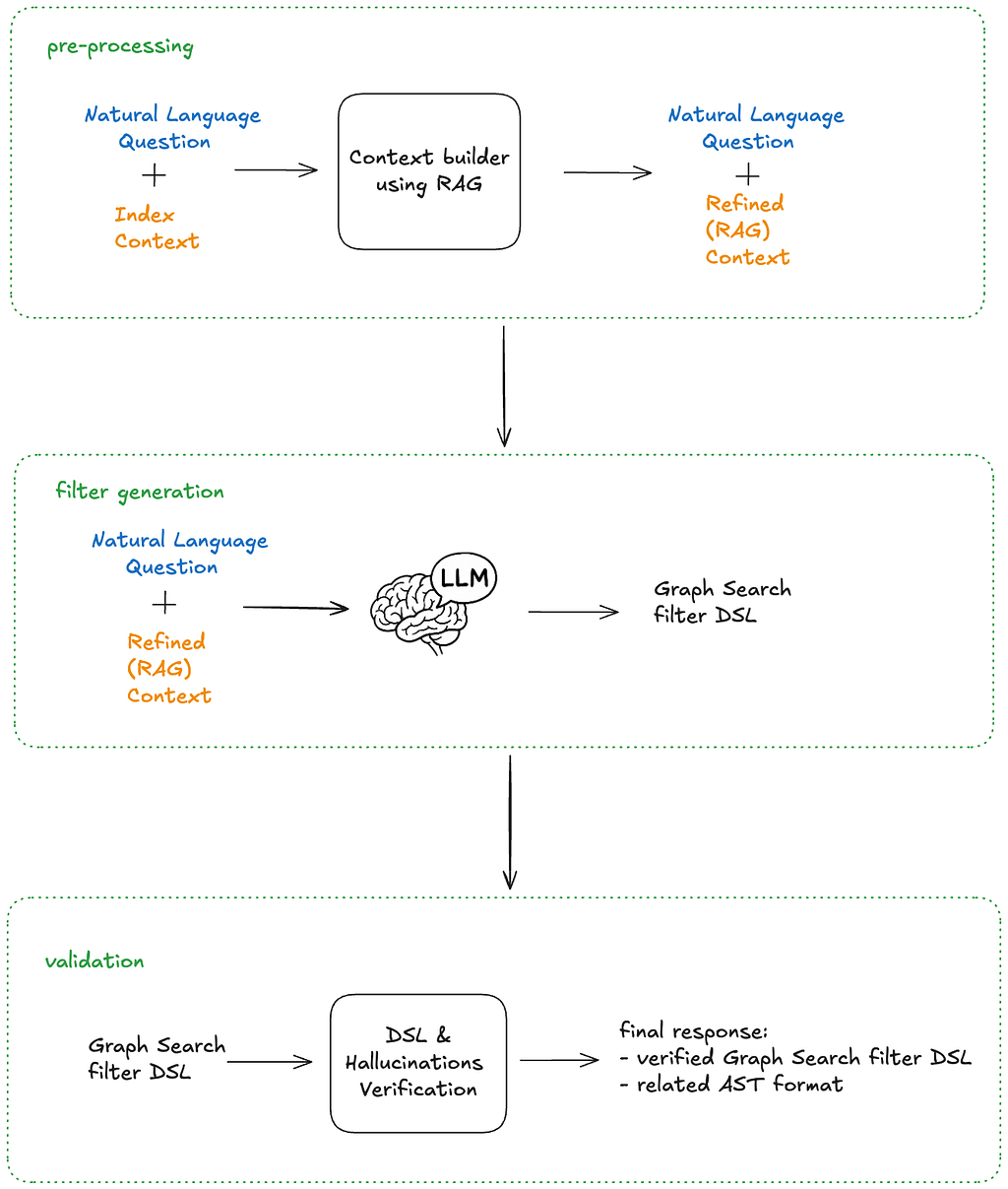
As mentioned previously, the solution architecture is divided into pre-processing, filter statement generation, and then post-processing stages. The pre-processing handles context building and involves a RAG pattern for similarity search, while the post-processing validation stage checks the correctness of the LLM-generated filter statements and provides visibility into the results for end users. This design strategically balances LLM involvement with more deterministic strategies.
End-to-end architecture
The end-to-end process is as follows:
A user’s natural language question (with optional `@mentions` statements) are provided as input, along with the Graph Search index context
The context is scoped by using the RAG pattern on both fields and possible values
The pre-processed context and the question are fed into the LLM with an instruction asking for a syntactically and semantically correct filter statement
The generated filer statement DSL is verified and checked for hallucinations
The final response contains the related AST in order to build “Chips” and “Facets”
Summary
By combining our existing Graph Search infrastructure with the power and flexibility of LLMs, we’ve bridged the gap between complex filter statements and user intent. We moved from requiring users to speak our language (DSL) to our systems understanding theirs.
The initial challenge for our users was successfully addressed. However, our next steps involve transforming this system into a comprehensive and expandable platform, rigorously evaluating its performance in a live production environment, and expanding its capabilities to support GraphQL-first user interfaces. These topics, and others, will be the focus of the subsequent installments in this series. Be sure to follow along!
You may have noticed that we have a lot more to do on this project, including named entity recognition and extraction, intent detection so we can route questions to the appropriate indices, and query rewriting among others. If this kind of work interests you, reach out! We’re hiring in our Warsaw office, check for open roles here.
With CloudHSM, you can manage and access your keys on FIPS 140-3 Level 3 validated hardware, protected with customer-owned, single-tenant hardware security module (HSM) instances that run in your own virtual private cloud (VPC). This PCI PIN attestation gives you the flexibility to deploy your regulated workloads with reduced compliance overhead. CloudHSM might be suitable when operations supported by the service are integrated into a broader solution that requires PCI-PIN compliance. For payment operations, such as PIN translation, we encourage you to consider AWS Payment Cryptography as a fully managed alternative for PCI-PIN compliance.
The PCI PIN compliance report package for AWS CloudHSM includes two key components:
PCI PIN Attestation of Compliance (AOC) – demonstrating that AWS CloudHSM was successfully validated against the PCI PIN standard with zero findings
PCI PIN Responsibility Summary – provides guidance to help AWS customers understand their responsibilities in developing and operating a highly secure environment for handling PIN-based transactions
AWS was evaluated by Coalfire, a third-party Qualified Security Assessor (QSA). Customers can access the PCI PIN Attestation of Compliance (AOC) and PCI PIN Responsibility Summary reports through AWS Artifact.
To learn more about our PCI program and other compliance and security programs, see the AWS Compliance Programs page. As always, we value your feedback and questions; reach out to the AWS Compliance team through the Contact Us page.
If you have feedback about this post, submit comments in the Comments section below. If you have questions about this post, contact AWS Support.
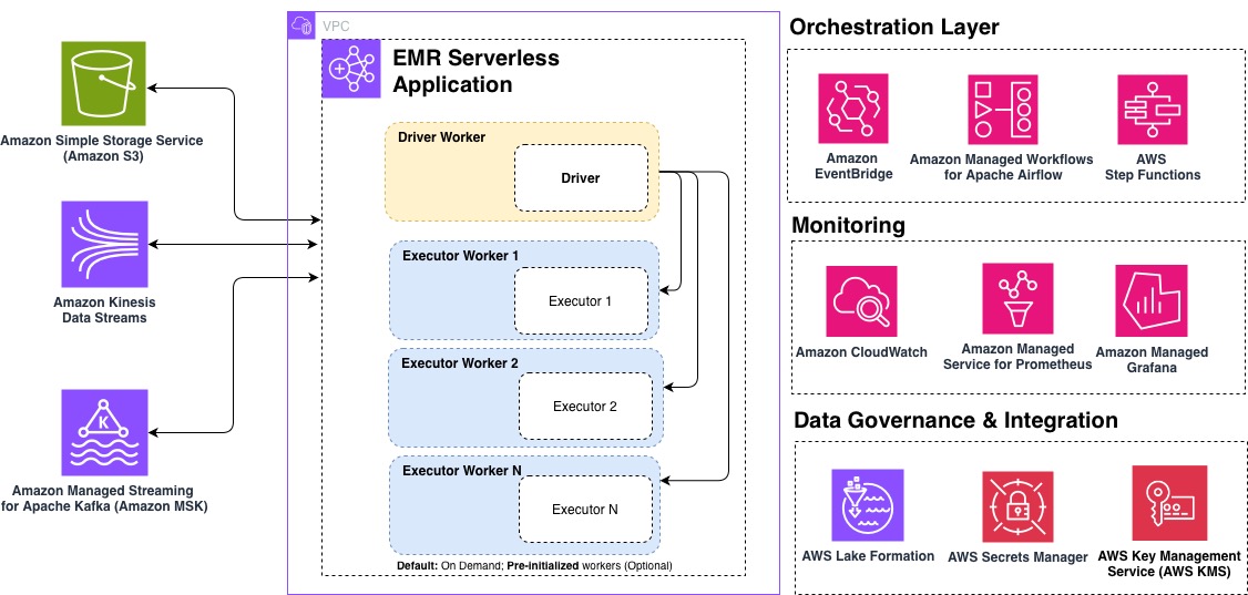
Amazon EMR Serverless is a deployment option for Amazon EMR that you can use to run open source big data analytics frameworks such as Apache Spark and Apache Hive without having to configure, manage, or scale clusters and servers. EMR Serverless integrates with Amazon Web Services (AWS) services across data storage, streaming, orchestration, monitoring, and governance to provide a comprehensive serverless analytics solution.
In this post, we share the top 10 best practices for optimizing your EMR Serverless workloads for performance, cost, and scalability. Whether you’re getting started with EMR Serverless or looking to fine-tune existing production workloads, these recommendations will help you build efficient, cost-effective data processing pipelines. The following diagram illustrates an end-to-end EMR Serverless architecture, showing how it integrates into your analytics pipelines.
1. Define applications one time, reuse multiple times
EMR Serverless applications function as cluster templates that instantiate when jobs are submitted and can process multiple jobs without being recreated. This design significantly reduces startup latency for recurring workloads and simplifies operational management.
Typical workflow for EMR on EC2 transient cluster:
Typical workflow for EMR Serverless:
Applications feature a self-managing lifecycle that provisions resources to be available when needed without manual intervention. They automatically provision capacity when a job is submitted. For applications without pre-initialized capacity, resources are released immediately after job completion. For applications with pre-initialized capacity configured, those pre-initialized workers will stop after exceeding the configured idle timeout (15 minutes by default). You can adjust this timeout at the application level using AutoStopConfig configuration in the CreateApplication or UpdateApplication API. For example, if your jobs run every 30 minutes, increasing the idle timeout can eliminate startup delays between executions.
Most workloads are suited for on-demand capacity provisioning, which automatically scales resources based on your job requirements without incurring charges when idle. This approach is cost-effective and suitable for typical use cases including extract, transform, and load (ETL) workloads, batch processing jobs, and scenarios requiring maximum job resiliency.
For specific workloads with strict instant-start requirements, you can optionally configure pre-initialized capacity. Pre-initialized capacity creates a warm pool of drivers and executors that are ready to run jobs within seconds. However, this performance advantage comes with a tradeoff of added cost because pre-initialized workers incur continuous charges even when idle until the application reaches the Stopped state. Additionally, pre-initialized capacity restricts jobs to a single Availability Zone, which reduces resiliency.
Pre-initialized capacity should only be considered for:
Time-sensitive jobs with sub second service level agreement (SLA) requirements where startup latency is unacceptable
Interactive analytics where user experience depends on instant response
High-frequency production pipelines running every few minutes
In most other cases, on-demand capacity provides the best balance of cost, performance, and resiliency.
Beyond optimizing your applications’ use of resources, consider how you organize them across your workloads. For production workloads, use separate applications for different business domains or data sensitivity levels. This isolation improves governance and prevents resource contention between critical and noncritical jobs.
Selecting the right underlying processor architecture can significantly impact both performance and cost. Graviton ARM-based processors offer significant performance improvement compared to x86_64.
EMR Serverless automatically updates to the latest instance generations as they become available, which means your applications benefit from the newest hardware improvements without requiring additional configuration.
To use Graviton with EMR Serverless, specify ARM64 with the architecture parameter during application creation using the CreateApplication or with the UpdateApplication API for existing applications:
Resource availability – For large-scale workloads, consider engaging with your AWS account team to discuss capacity planning for Graviton workers.
Compatibility – Although many commonly used and standard libraries are compatible with Graviton (arm64) architecture, you will need to validate that third-party packages and libraries used are compatible.
Migration planning – Take a strategic approach to Graviton adoption. Build new applications on ARM64 architecture by default and migrate existing workloads through a phased transition plan that minimizes disruption. This structured approach will help optimize cost and performance without compromising reliability.
Workers are used to execute the tasks for your workload. While EMR Serverless defaults are optimized out of the box for a majority of use cases, you may need to right-size your workers to improve processing time and optimize cost efficiency. When submitting EMR Serverless jobs, it’s recommended to define Spark properties to configure workers, including memory size (in GB) and number of cores.
EMR Serverless configures the default worker size of 4 vCPUs, 16 GB memory, and 20 GB disk. Although this generally provides a balanced configuration for most jobs, you might want to adjust the size based on your performance requirements. Even when configuring pre-initialized workers with specific sizing, always set your Spark properties at job submission. This allows your job to use the specified worker sizing rather than default properties when it scales beyond pre-initialized capacity. When right-sizing your Spark workload, it’s important to identify the vCPU:memory ratio for your job. This ratio determines how much memory you allocate per virtual CPU core in your executors. Spark executors need both CPU and memory to process data effectively, and the optimal ratio varies based on your workload characteristics.
To get started, use the following guidance, then refine your configuration based on your specific workload requirements.
Executor configuration
The following table provides recommended executor configurations based on common workload patterns:
To further monitor and tune your configuration, monitor your workload’s resource consumption using Amazon CloudWatch job worker-level metrics to identify constraints. Track CPU utilization, memory usage, and disk utilization metrics, then use the following table to fine-tune your configuration based on observed bottlenecks.
Metrics observed
Workload type
Suggested action
1
High memory (>90%), Low CPU (<50%)
Memory-bound workload
Increase vCPU:memory ratio
2
High CPU (>85%), low memory (<60%)
CPU-bound workload
Increase vCPU count, maintain 1:4 ratio (For example, if using 8 vCPU, use 32 GB memory)
3
High storage I/O, normal CPU or memory with long shuffle operations
**You can identify frequent garbage collect (GC) pauses using the Spark UI under the Executors tab. There will be a GC time column that should generally be less than 10% of task time. Alternatively, the driver logs might frequently contain GC (Allocation Failure)] messages.
4. Control scaling boundary with T-shirt sizing
By default, EMR Serverless uses dynamic resource allocation (DRA), which automatically scales resources based on workload demand. EMR Serverless continuously evaluates metrics from the job to optimize for cost and speed, removing the need for you to estimate the exact number of workers required.
For cost optimization and predictable performance, you can configure an upper scaling boundary using one of the following approaches:
Rather than trying to fine-tune spark.dynamicAllocation.maxExecutors to an arbitrary value for each job, you can think about setting this configuration as t-shirt sizes that represent different workload profiles:
Workload size
Use cases
spark.dynamicAllocation.maxExecutors
Small
Exploratory queries, development
50
Medium
Regular ETL jobs, reports
200
Large
Complex transformations, large-scale processing
500
This t-shirt sizing approach simplifies capacity planning and helps you balance performance with cost efficiency based on your workload category, rather than attempting to optimize each individual job.
For EMR Serverless releases 6.10 and above, the default value for spark.dynamicAllocation.maxExecutors is infinity, but for earlier releases, it’s 100.
EMR Serverless automatically scales workers up or down based on the workload and parallelism required at every stage of the job. This automatic scaling is continuously evaluating metrics from the job to optimize for cost and speed, which removes the need for you to estimate the number of workers that the application needs to run your workloads.
However, in some cases, if you have a predictable workload, you might want to statically set the number of executors. To do so, you can disable DRA and specify the number of executors manually:
5. Provision appropriate storage for EMR Serverless jobs
Understanding your storage options and sizing them appropriately can prevent job failures and optimize execution times. EMR Serverless offers multiple storage options to handle intermediate data during job execution. The storage option selected will depend on the EMR release and use case. The storage options available in EMR Serverless are:
Storage type
EMR release
Disk size range
Use case
Benefits
Serverless Storage (recommended)
7.12+
N/A (auto-scaling)
Most Spark workloads, especially data-intensive workloads
No storage costs
auto-scaling
Reduces disk failures
Up to 20% cost reduction
Standard Disks
7.11 and lower
20–200 GB per worker
Small to medium workloads processing datasets under 10 TB
Simple configuration
20 GB default suitable for most workloads,
200 GB max for optimal throughput
Shuffle-Optimized Disks
7.1.0+
20–2,000 GB per worker
Large-scale ETL workloads processing multi-TB
High IOPS and throughput
Up to 2 TB capacity per worker
By matching your storage configuration to your workload characteristics, you’ll enable EMR Serverless jobs to run efficiently and reliably at scale.
6. Multi-AZ out-of-the-box with built-in resiliency
EMR Serverless applications are multi-AZ from the start when pre-initialized capacity isn’t enabled. This built-in failover capability provides resilience against Availability Zone disruptions without manual intervention. A single job will operate within a single Availability Zone to prevent cross-AZ data transfer costs and subsequent jobs will be intelligently distributed across multiple AZs. If EMR Serverless determines that an AZ is impaired, it will submit new jobs to a healthy AZ, enabling your workloads to continue running despite AZ impairment.
To fully benefit from EMR Serverless multi-AZ functionality verify the following:
Avoid pre-initialized capacity which restricts applications to a single AZ
Make sure there are sufficient IP addresses available in each subnet to support the scaling of workers
In addition to multi-AZ, with Amazon EMR 7.1 and higher, you can enable job resiliency, which allows your jobs to be automatically retried in case errors are encountered. If there are multiple Availability Zones configured, it will also be retried in a different AZ. You can enable this feature for both batch and streaming jobs, though retry behavior differs between the two.
Configure job resiliency by specifying a retry policy that defines the maximum number of retry attempts. For batch jobs, the default is no automatic retries (maxAttempts=1). For streaming jobs, EMR Serverless retries indefinitely with built-in thrash prevention that stops retries after five failed attempts within 1 hour. You can configure this threshold between 1–10 attempts. For more information, refer to Job resiliency.
In the event that you need to cancel your job, you can specify a grace period to allow your jobs to shut down cleanly rather than the default behavior of immediate termination. This can also include custom shutdown hooks if you need to perform custom cleanup actions.
By combining multi-AZ support, automatic job retries, and graceful shutdown periods, you create a robust foundation for EMR Serverless workloads that can tolerate interruptions and maintain data integrity without manual intervention.
7. Secure and extend connectivity with VPC integration
When configuring VPC access for your EMR Serverless application, keep these key considerations in mind to gain optimal performance and cost efficiency:
Plan for sufficient IP addresses – Each worker uses one IP address within a subnet. This includes the workers that will be launched when your job is scaling out. If there aren’t enough IP addresses, your job might not be able to scale, which could result in job failure. Verify you have adhered to best practices for subnet planning for optimal performance.
Set up Gateway endpoints for Amazon S3 for applications in a private subnets – Running EMR Serverless in a private subnet without VPC endpoints for Amazon S3 will route your Amazon S3 traffic through NAT gateways, resulting in additional data transfer charges. VPC endpoints for S3 will keep this traffic within your VPC, reducing costs and improving performance for Amazon S3 operations.
Manage AWS Config costs for network interfaces – EMR Serverless generates an elastic network interface record in AWS Config for each worker, which can accumulate costs as your workloads scale. If you don’t require AWS Config tracking for EMR Serverless network interfaces, consider using resource-based exclusions or tagging strategies to filter them out while maintaining AWS Config coverage for other resources.
8. Simplify job submission and dependency management
EMR Serverless supports flexible job submission through the StartJobRun API, which accepts the full spark-submit syntax. For runtime environment configuration, use the spark.emr-serverless.driverEnv and spark.executorEnv prefixes to set environment variables for driver and executor processes. This is particularly useful for passing sensitive configuration or runtime-specific settings.
For Python applications, package dependencies using virtual environments by creating a venv, packaging it as a tar.gz archive, or uploading to Amazon S3 using spark.archives with the appropriate PYSPARK_PYTHON environment variable. This allows Python dependencies to be available across driver and executor workers.
For improved control under high load, enable job concurrency and queuing (available in EMR 7.0.0+) to limit the number of jobs that can be executed concurrently. With this feature, jobs submitted that exceed the concurrency limit are queued until resources become available.
9. Use EMR Serverless configurations to enforce limits
EMR Serverless automatically scales resources based on workload demand, providing optimized defaults that work well for most use cases without requiring Spark configuration tuning. To manage costs effectively, you can configure resource limits that align with your budget and performance requirements. For advanced use cases, EMR Serverless also provides configuration options so you can fine-tune resource consumption and achieve the same efficiency as cluster-based deployments. Understanding these limits helps you balance performance with cost efficiency for your jobs.
Limit type
Purpose
How to configure
Job-level
Control resources for individual jobs
spark.dynamicAllocation.maxExecutors or spark.executor.instances
Application-level
Limit resources per application or business domain
Set maximum capacity when creating the application or while updating.
Account-level
Prevent abnormal resource spikes across all applications
These three layers of limits work together to provide flexible resource management at different scopes. For most use cases, configuring job-level limits using the t-shirt sizing approach is sufficient, while application and account-level limits provide additional guardrails for cost control.
10. Monitor with CloudWatch, Prometheus, and Grafana
Monitoring EMR Serverless workloads simplifies the process of debugging, performing cost optimization, and performance tracking. EMR Serverless offers three tiers of monitoring that work together: Amazon CloudWatch, Amazon Managed Service for Prometheus, and Amazon Managed Grafana.
Amazon CloudWatch – CloudWatch integration is enabled by default and publishes metrics to the AWS/EMRServerless namespace. EMR Serverless sends metrics to CloudWatch every minute at the application level, as well as job, worker-type, and capacity-allocation-type levels. Using CloudWatch, you can configure dashboards for enhanced observability into workloads or configure alarms to alert for job failures, scaling anomalies, and SLA breaches. Using CloudWatch with EMR Serverless provides insights to your workloads so you can catch issues before they impact users.
Amazon Managed Service for Prometheus – With EMR Serverless release 7.1+, you can enable Prometheus for detailed Spark engine metrics to push metrics to Amazon Managed Service for Prometheus. This unlocks executor-level visibility, including memory usage, shuffle volumes, and GC pressure. You can use this to identify memory-constrained executors, detect shuffle-heavy stages, and find data skew.
Amazon Managed Grafana – Grafana connects to both CloudWatch and Prometheus data sources, providing a single pane of glass for unified observability and correlation analysis. This layered approach helps you correlate infrastructure issues with application-level performance problems.
In this post, we shared 10 best practices to help you maximize the value of Amazon EMR Serverless by optimizing performance, controlling costs, and maintaining reliable operations at scale. By focusing on application design, right-sized workloads, and architectural choices, you can build data processing pipelines that are both efficient and resilient.
Customers often want to deploy Amazon OpenSearch Service domains in virtual private clouds (VPC) and use single sign-on (SSO) with SAML for access control to enhance security. However, setting this up can be challenging.
In this post, we explore different OpenSearch Service authentication methods and network topology considerations. Then we show how to build an architecture to access an OpenSearch Service domain hosted in a VPC using AWS Client VPN, AWS Transit Gateway, and AWS IAM Identity Center.
Solution overview
The following diagram illustrates the solution architecture.
The end-user authenticates with IAM Identity Center and connects to the AWS environment from their browser through Client VPN. The traffic is routed from the VPN VPC to the database VPC where the OpenSearch service endpoints are deployed. The user then authenticates to OpenSearch Service through IAM Identity Center. This architecture provides a scalable, enterprise-grade solution that avoids using bastion hosts while making sure only authorized users can access your OpenSearch Service domains through a secure VPN connection. In the following sections, we walk through the steps to set up IAM Identity Center, configure Transit Gateway to facilitate communication between VPCs, and configure SAML-based authentication using IAM Identity Center for both OpenSearch Service and VPN access. Prior experience setting up Client VPN, IAM Identity Center, and Transit Gateway would be beneficial but is not necessary to follow along with this post.
OpenSearch Service authentication methods and SAML
OpenSearch Service supports multiple authentication methods. You can use AWS Identity and Access Management (IAM) to call the OpenSearch Service configuration API (for details, see Making and signing OpenSearch Service requests). However, this doesn’t give you access to the visual dashboard. To access the visual dashboard and call the OpenSearch Service configuration API, you can use the OpenSearch Service built-in internal user database or Amazon Cognito for authentication and user management features. However, these options use separate user pools, which adds additional security and management overhead when adding and removing users.
Therefore, many customers choose to use SAML federation to integrate OpenSearch Service authentication with their existing identity providers like Entra ID, Okta, or JumpCloud. For this post, we use the IAM Identity Center directory as our identity source. One limitation of this approach is that it only supports identity provider-initiated authentication. This means that users must log in through the IAM Identity Center portal and then access their OpenSearch Service dashboard from there.
Private network topology options for OpenSearch Service
When deploying OpenSearch Service domains in a private VPC, organizations must establish secure and reliable network connectivity to access their OpenSearch Service domains. AWS offers several networking solutions that can be implemented individually or in combination to meet specific access requirements. These options include Transit Gateway for centralized network management, AWS Direct Connect or AWS Site-to-Site VPN for on-premises connectivity, and Client VPN for secure remote access. Each solution provides unique benefits and can be combined to meet different organizational needs, security requirements, and performance expectations.
AWS Transit Gateway
Transit Gateway functions as a cloud router that simplifies network connectivity by acting as a central hub for connecting VPCs and on-premises networks. Implementing Transit Gateway with OpenSearch Service enables consolidated access to your OpenSearch Service domain across multiple VPCs and AWS accounts. Through Transit Gateway route tables, you can precisely control traffic flow between attached networks. It supports transitive routing between VPCs and on-premises networks, significantly reducing the number of peering connections needed to access your OpenSearch Service domain. This centralized approach is a common pattern used by customers, which makes network management scalable as your infrastructure grows.
AWS Client VPN
With Client VPN, you can securely access your private OpenSearch Service domain through a managed OpenVPN-based solution. Using Client VPN removes the need to use a bastion host or proxy server to access an OpenSearch Service domain, reducing your management burden and improving security. Client VPN supports both certificate-based and SAML-based authentication. Client VPN endpoints can be associated with multiple subnets to provide high availability. The service includes comprehensive security features such as connection logging and security group controls.
Combining Client VPN with Transit Gateway provides a scalable and flexible way to access an OpenSearch Service domain in a private VPC. In the subsequent sections, we walk you through how to integrate the various services.
Prerequisites
If you haven’t yet set up IAM Identity Center, refer to Enable IAM Identity Center to enable it. Both organization instances and account instances will work. The Identity Center instance must be deployed in the same AWS Region as your OpenSearch Service domain.
After you set up IAM Identity Center, complete the following steps to create an IAM Identity Center group:
On the IAM Identity Center console, choose Groups in the navigation pane.
Choose Create group and create a group (for this example, we name the group vpn_users.
After you create the group, choose the group name to open its details page.
Locate the group ID under General information. Save this in a text editor.
Create a user (or multiple users) and assign them to the vpn_users group. This can be done directly through the user creation flow or after creating the user.
Set up the initial network topology
For this post, we use the network topology shown in the following diagram. One VPC hosts the client VPN endpoint with CIDR range 10.0.0.0/16 and a separate VPC with CIDR range 10.1.0.0/16 that hosts our OpenSearch Service nodes. The two VPCs are connected with Transit Gateway. The CIDR ranges in your environment may vary. The only requirement is that they can’t overlap.
Next, you must update each VPC route table to facilitate connectivity to the OpenSearch Service domain.
On the Amazon VPC console, choose Route tables in the navigation pane.
For VPN-VPC, add routes on the subnets where the Client VPN endpoints are attached. The route is 10.1.0.0/16 using Transit Gateway. This route allows VPN users to reach Database-VPC.
For Database-VPC, add routes on the subnets of the OpenSearch Service domain endpoint. The route is 10.0.0.0/16 using Transit Gateway. This route allows responses from Database-VPC back to reach the VPN users.
Next, you must update the Transit Gateway Security Group Referencing support configuration. This allows the OpenSearch Service domain’s security group to open port 443 to only the Client VPN security group. This makes applying least privilege simpler.
On the Transit Gateway console, select the transit gateway you’re using.
On the Actions menu, choose Modify transit gateway.
Select Security Group Referencing support and choose Modify transit gateway.
Configure Client VPN authentication
Client VPN can be associated to multiple VPC subnets for high availability. Client VPN supports multiple client authentication methods. For this post, we use SAML-based authentication with IAM Identity Center.
To set up SAML-based authentication with IAM Identity Center, follow the instructions in the following sections. For more details, refer to Authenticate AWS Client VPN users with AWS IAM Identity Center. Deploy and associate the Client VPN endpoint with VPN-VPC.
Configure Client VPN access to database VPC
During the initial setup of the Client VPN endpoint, you defined authorization rules that authorized the VPN_users group to access the VPN-VPC network, which is 10.0.0.0/16.Complete the following steps to add connectivity to database-VPC:
On the Amazon VPC console, choose Client VPC endpoints in the navigation pane.
Select the endpoint you created.
In the Authorization rules section, choose Add authorization rules.
For Destination network to enable access, enter 10.1.0.0/16 (this is the database VPC).
For Grant access to, select Allow access to all users.
Choose Add authorization rule.
After you create the authorization rule, the user now has access to that CIDR range. Next, you add an entry in the Client VPN endpoint’s route table to provide reachability from a network perspective.
On the Client VPN endpoints page, select the endpoint you just created.
In the Route table section, choose Create route.
For Route destination, enter the CIDR range for Database-VPC (10.1.0.0/16).
For Subnet ID for target network association, choose a subnet ID.
Choose Create route.
You should see the new route in the “Creating” state. After it has reached the “Active” state, VPN users will have a network path to the database VPC to be able to reach the OpenSearch Service domain.
Configure Client VPN application on your client
Complete the following steps to configure the Client VPN application to your client:
Download the relevant installer for Client VPN for Desktop and install Client VPN.
Download and prepare the Client VPN endpoint file.
Open the Client VPN application.
Choose Manage Profile, then choose Add Profile.
Enter a display name and upload the VPN configuration file.
Choose Add Profile.
Set up federation with IAM Identity Center with OpenSearch Service
Complete the following steps to set up federation with IAM Identity Center with OpenSearch Service:
Set up the SAML integration between OpenSearch Service and IAM Identity Center. Assign the same groups that you assigned to the VPN custom application to the OpenSearch Service custom application.
Modify the security group associated with the OpenSearch Service domain to allow access from the Client VPN subnet.
Modify the security group of Client VPN and add the following entry:
Type: HTTPS
Source: Use Custom and reference the security group of the OpenSearch Service domain
Test the end-to-end flow
Now you can test the entire flow end-to-end:
Run Client VPN on your local machine. Use the profile that you previously configured. The client will prompt you to authenticate with IAM Identity Center. After authentication, you will see the message “Authentication details received, processing details. You may close this window at any time.”
Access your IAM Identity Center access portal URL (this can be found on the IAM Identity Center console, under Dashboard). Sign in as a user that has been assigned to the OpenSearch Service custom application in the previous step.
After authentication, choose the Applications tab in AWS Access Portal and choose the OpenSearch Service application.
This should redirect you to the OpenSearch Service Dashboards page with the role that you assigned.
Clean up
After you test the solution, delete the resources you created to avoid incurring future charges:
Delete the OpenSearch Service domain and the SAML application, users, and groups in IAM Identity Center.
Delete the client VPN endpoints that you created and remove the routing rules from Transit Gateway.
Conclusion
In this post, we discussed the networking options for securely accessing an OpenSearch Service domain deployed in a private VPC through services like Transit Gateway, Client VPN, and Site-to-Site VPN. We also discussed how to use IAM Identity Center for authentication and authorization, helping you simplify identity management for OpenSearch Service. If you have feedback about this post, provide it in the comments section.
Organizations increasingly depend on trusted, high-quality data to drive analytics, regulatory reporting, and operational decision-making. When data quality issues go undetected, they can lead to inaccurate insights, stalled initiatives, and compliance gaps that directly affect business outcomes. As data volumes grow and pipelines become more distributed, maintaining consistent data quality across teams and data domains becomes progressively more challenging.
You can address these challenges with AWS Glue Data Quality by providing automated, rule-based data validation across datasets in the AWS Glue Data Catalog and within AWS Glue ETL pipelines. With the Data Quality Definition Language (DQDL), you can author both straightforward and advanced validation rules to detect data quality issues early in the lifecycle, before they reach downstream applications or analytics environments.
In this post, we highlight the new DQDL labels feature, which enhances how you organize, prioritize, and operationalize your data quality efforts at scale. We show how labels such as business criticality, compliance requirements, team ownership, or data domain can be attached to data quality rules to streamline triage and analysis. You’ll learn how to quickly surface targeted insights (for example, “all high-priority customer data failures owned by marketing” or “GDPR-related issues from our Salesforce ingestion pipeline”) and how DQDL labels can help teams improve accountability and accelerate remediation workflows.
Managing complex data quality rules across teams and use cases
As organizations advance in their data quality programs, a few rules often grow into hundreds or thousands maintained across many teams and business domains. Take the example of AnyCompany, a large retail organization with multiple data teams managing customer, product, and sales data across different business units. These teams run a variety of data quality rules, including weekly customer checks, daily product validations, frequent sales checks, and monthly compliance reviews, with different naming patterns, schedules, and response processes. This creates a fragmented, hard-to-navigate system where teams operate in isolation and data quality practices become inconsistent.
The challenge lies in the volume of rules and the lack of organizational context around them. When dozens of data quality rules pass or fail, teams still lack clarity on ownership, urgency, or business impact. This slows incident response, limits executive insight, and complicates resource planning. To move from technical monitoring to strategic value, organizations need a unified structure that connects data quality rules to teams, domains, and priorities, bringing essential business context to data quality operations.
Metadata-driven rule organization
AWS Glue DQDL labels address organizational challenges because you can attach custom metadata to data quality rules, transforming anonymous validations into contextually rich, business-aware checks. Labels work as key-value pairs attached to individual rules or entire rule sets, and you can organize quality operations around business dimensions such as team ownership, criticality, frequency, and regulatory requirements, as in the case of the AnyCompany example. When a rule fails, you immediately identify what failed, who should respond, how urgent it is, and which business area is affected, whether it’s the marketing department tracking email completeness with daily frequency tags, compliance teams monitoring age verification with regulation labels, or the finance team validating payment data with high-criticality markers.
Labels integrate with existing DQDL syntax without requiring changes to current rule definitions, working consistently across AWS Glue Data Quality execution contexts. The feature’s flexibility supports organizational taxonomies from cost centers and geographic regions to data sensitivity levels and service-level agreement (SLA) requirements with single rules carrying multiple labels simultaneously for sophisticated filtering and analysis. Labels appear in the outputs, including rule outcomes, row-level results, and API responses, so organizational context travels with quality results whether you’re troubleshooting failures, analyzing trends in Amazon Athena, or building executive dashboards in Amazon Quick Sight.
Getting started: Writing your first labeled data quality rules
Let’s walk through creating your first labeled data quality rules using AnyCompany’s customer data scenario. We’ll use their customer demographics dataset, which contains customer information that multiple teams need to validate with different priorities and frequencies.
DQDL labels follow a straightforward key-value pair syntax that integrates naturally with existing rule definitions. The basic syntax supports two approaches: default labels that apply to the rules in a rule set, and rule-specific labels that apply to individual rules. Rule-specific labels can override default labels when using the same key, providing fine-grained control over your labeling strategy.
When implementing DQDL labels, keep the following constraints in mind:
Maximum of 10 labels per rule
Label keys are limited to 128 characters and can’t be empty
Label values are limited to 256 characters and can’t be empty
Both keys and values are case-sensitive
Rule-specific labels override default labels when using the same key
Using this labeling approach, you can organize and manage data quality rules efficiently across different teams and validation requirements.
Best practices for label naming conventions
Here are some proven labeling strategies that scale across enterprise environments:
Establish a complete standardized taxonomy upfront – Define label keys in DefaultLabels with sensible defaults such as regulation=none or sla=24h to provide rules with identical keys for cross-team queries.
Use consistent key naming patterns – Establish standard keys such as team, criticality, sla, impact, and regulation across rule sets to maintain query consistency.
Implement hierarchical values – Use formats such as team=marketing-analytics to support both broad and specific filtering while keeping key structure consistent.
Include operational metadata in defaults – Define labels such as sla, escalation-level, or notification-channel as defaults to drive automated response workflows.
Plan for reporting dimensions – Include keys such as cost-center, region, or business-unit in your default taxonomy to support meaningful business analytics.
Use standardized value patterns – Establish consistent formats such as criticality=high/medium/low or sla=15m/1h/1d for predictable filtering and sorting.
These are guidelines rather than requirements but following them from the start enables powerful cross-team analytics and reduces future refactoring effort.
Customer data validation hands-on example
This post assumes you’re familiar with AWS Glue Data Quality and ETL operations. Using the following hands-on walkthrough, you’ll learn how to implement DQDL labels for organizational data quality management.
Start by establishing default labels that automatically apply to every rule in the rule set, providing consistent organizational context:
DefaultLabels provide a foundational taxonomy that automatically propagates across your entire rule set, creating uniformity and reducing configuration overhead. By defining default values at the organizational level, such as team=data-team, criticality=medium, regulation=none, sla=24h, and impact=medium, every rule inherits these standardized attributes without requiring explicit declaration. This inheritance model promotes consistency while maintaining the flexibility individual teams need to address their unique operational contexts.
Individual teams can selectively override inherited defaults to reflect their specific requirements. For example, examine the following complete rule set:
Notice how the compliance team changes regulation from 'none' to 'age21' for age verification rules and analytics elevates criticality to 'high' for business-critical checks. Unspecified labels automatically inherit the default values, providing consistency while maintaining team-level flexibility.
Applying labeled rules against the dataset
Now let’s see DQDL labels in action by applying AnyCompany’s rule set to actual data through an AWS Glue ETL pipeline. This section assumes you’re familiar with AWS Glue EvaluateDataQuality transform and basic extract, transform, and load (ETL) job creation.
We use AWS Glue EvaluateDataQuality transform within an ETL job to process our customer dataset and apply our labeled rule set. The transform generates two types of outputs: rule-level outcomes that show which rules passed or failed with their associated labels and row-level results that identify specific records and the labeled rules they violated.
By default, labels are excluded from row-level results. However, by enabling them you can analyze data quality results at both the individual record level and across organizational dimensions such as teams and criticality levels.
To enable labels in row-level results, you must configure the additionalOptions parameter in your EvaluateDataQuality transform. The key setting is "rowLevelConfiguration.ruleWithLabels":"ENABLED", which instructs AWS Glue to include label metadata for each rule evaluation at the individual record level.
Here’s how to implement an ETL pipeline that applies our AnyCompany’s rule set with labels enabled:
To run this example, update the s3_bucket variable with your own Amazon Simple Storage Service (Amazon S3) bucket name, then create and execute the ETL job in AWS Glue.
After the job is completed, you’ll find:
Rule-level and row-level results stored in your S3 bucket
Two new tables automatically created in your default database: dqrulelevel and dqrowlevel
In the next section, we query these tables using Amazon Athena to analyze the labeled data quality outcomes and extract actionable insights.
Analyzing data quality results by labels using Amazon Athena
We’ve stored our labeled data quality results in Amazon S3 and as a table in the AWS Glue data catalog. Now, we can use Amazon Athena to analyze these results across the organizational dimensions captured in your labels. The labeled metadata transforms raw data quality outcomes into actionable business intelligence that drives targeted remediation and strategic decision-making.
Querying row-level results
With labels stored alongside row-level outcome, you can query specific records that failed data quality checks based on label criteria. For example, the following query identifies individual customer records that failed high criticality compliance rules. You can use it to quickly locate and remediate problematic data for regulatory or business-critical use cases:
SELECT
c_customer_id,
c_age,
failed_rule
FROM (
SELECT *
FROM dqrowlevel
WHERE dataqualityevaluationresult = 'Failed'
)
CROSS JOIN UNNEST(dataqualityrulesfail) AS t(failed_rule)
WHERE failed_rule LIKE '%criticality"="high"%'
AND failed_rule LIKE '%team"="compliance"%'
LIMIT 5;
You can see the query results above showing failed records filtered by 'high' criticality and 'compliance' team labels.
Querying rule-level results
Now that we have stored rule-level outcomes with labels, we can run aggregation queries to analyze failures across different dimensions. For example, the following query groups failed rules by criticality and team to identify which teams have the most high-severity failures. You can use it to prioritize remediation efforts and allocate resources effectively:
SELECT
    labels['team'] AS team,
    labels['criticality'] AS criticality,
    COUNT(*) AS failed_count
FROM dqrulelevel
WHERE outcome = 'Failed'
GROUP BY labels['criticality'], labels['team']
ORDER BY failed_count DESC;
The following screenshot shows aggregated failure counts grouped by team and criticality level.
Viewing data quality results using AWS CLI
Beyond querying results in Athena, you can also retrieve data quality outcomes directly using the AWS Command Line Interface (AWS CLI). This is useful for automation, scripting, and integrating data quality checks into continuous integration and continuous delivery (CI/CD) pipelines.
To list data quality results for your ETL job, enter the following:
The output includes a Labels object for each rule in the RuleResults array, containing the label key-value pairs you defined. This provides programmatic access to the same labeled data quality results, which can be useful for automation and scripting workflows.
Cleanup
To avoid incurring ongoing charges, delete the resources created in this post:
To delete the S3 folders containing the data quality results, follow the directions at Deleting Amazon S3 objects.
To delete the ETL job you created for the test, follow the directions at Delete jobs in the AWS Glue User Guide.
To delete the AWS Glue Data Catalog dqrulelevel and dqrowlevel tables, follow the directions at DeleteTable in the AWS Glue Web API Reference.
Conclusion
AWS Glue DQDL labels add organizational context to data quality management by attaching business metadata directly to validation rules. This helps teams identify rule ownership, prioritize failures, and coordinate remediation efforts more effectively.Throughout this post, we’ve seen how AnyCompany moved from managing hundreds of generic rules to implementing a labeled system where data quality results include team ownership and business context. Marketing teams can identify their email validation failures, compliance teams can focus on regulatory violations, and finance teams can address payment-related issues without manual coordination.To implement DQDL Labels in your organization:
Start simple – Begin with basic organizational dimensions such as team ownership, criticality levels, and SLA requirements. Expand your labeling approach as needed.
Establish standards – Define your label taxonomy up front, including default values for unused dimensions. This consistency supports analytics across teams.
Integrate gradually – Add labels to existing rule sets during routine maintenance.
Use analytics – Apply the Athena query patterns from this post to build tools such as dashboards and alerting workflows.
Build smart automation – Explore creating alerts and notifications tailored to your business criticality and SLA definitions. For example, configure immediate notifications for high-criticality compliance failures while batching low-priority marketing issues into daily reports.
We look forward to seeing how you implement DQDL labels in your organization and expand beyond the examples we’ve covered here. To dive into the AWS Glue Data Quality APIs, refer to Data Quality API documentation. To learn more about AWS Glue Data Quality, check out AWS Glue Data Quality.
Amazon EMR Serverless now supports Apache Spark 4.0.1 in preview, making analytics accessible to more users, simplifying data engineering workflows, and strengthening governance capabilities. The release introduces ANSI SQL compliance, VARIANT data types support for JSON handling, Apache Iceberg v3 table format support, and enhanced streaming capabilities. This preview is available in all regions where EMR Serverless is available.
In this post, we explore key benefits, technical capabilities, and considerations for getting started with Spark 4.0.1 on Amazon EMR Serverless—a serverless deployment option that simplifies running open-source big data frameworks, without requiring managing clusters. With the emr-spark-8.0-preview release label, you can evaluate new SQL capabilities, Python API improvements, and streaming enhancements in your existing EMR Serverless environment.
Benefits
Spark 4.0.1 helps you solve data engineering problems with specific improvements. This section shows how new capabilities help with real-world scenarios.
Make analytics accessible to more users
Simplify Extract Transform Load (ETL) development with SQL scripting. Data engineers often switch between SQL and Python to build complex ETL logic with control flow. SQL scripting in Spark 4.0.1 enables loops, conditionals, and session variables directly in SQL, reducing context-switching and simplifying pipeline development. Use pipe syntax (|>) to chain operations for more readable, maintainable queries.
Improve data quality with ANSI SQL mode. Silent type conversion failures can introduce data quality issues. ANSI SQL mode (now default) enforces standard SQL behavior, raising errors for invalid operations instead of producing unexpected results. Important: ANSI SQL mode is now enabled by default. Test your queries thoroughly during this preview evaluation.
Simplify data engineering workflows
Process JSON data efficiently with VARIANT. Teams working with semi-structured data often see slow performance from repeated JSON parsing. The VARIANT data type stores JSON in an optimized binary format, eliminating parsing overhead. You can efficiently store and query JSON data in data lakes without schema rigidity.
Build Python data sources without Scala. Integrating custom data sources previously required Scala expertise. The Python data Source API lets you build connectors entirely in Python, using existing Python skills and libraries without learning a new language.
Debug streaming applications with queryable state. Troubleshooting stateful streaming applications has historically required indirect methods. The new state data source reader shows streaming state as queryable DataFrames. You can inspect state during debugging, test state values in unit tests, and diagnose production incidents.
Strengthen governance capabilities
Establish comprehensive audit trails with Apache Iceberg v3. The Apache Iceberg v3 table format provides transaction guarantees and tracks data changes over time, giving you the audit trails needed for regulatory compliance. When combined with VARIANT data type support, you can maintain governance controls while handling semi-structured data efficiently in data lakes.
Key capabilities
Spark 4.0.1 Preview on EMR Serverless introduces four major capability areas:
The following sections provide technical details and code examples for each capability.
SQL enhancements
Spark 4.0.1 introduces new SQL capabilities including ANSI mode compliance, SQL UDFs, pipe syntax for readable queries, VARIANT type for JSON handling, and SQL scripting with control flow.
ANSI SQL mode by default
ANSI SQL mode is now enabled by default, enforcing standard SQL behavior for data integrity. Silent casting of out-of-range values now raises errors rather than producing unexpected results. Existing queries may behave differently, particularly around null handling, string casting, and timestamp operations. Use spark.sql.ansi.enabled=false if you need legacy behavior during migration.
SQL pipe syntax
You can now chain SQL operations using the |> operator for improved readability. The following example shows how you can replace nested subqueries with a more maintainable pipeline:
FROM customer
|> LEFT OUTER JOIN orders ON c_custkey = o_custkey
|> AGGREGATE COUNT(o_orderkey) c_count GROUP BY c_custkey
|> AGGREGATE COUNT(*) AS custdist GROUP BY c_count
|> ORDER BY custdist DESC
This replaces nested subqueries, making complex transformations easier to understand and maintain.
VARIANT data type
The VARIANT type handles semi-structured JSON/XML data efficiently without repeated parsing. It uses an optimized binary representation internally while maintaining schema-less flexibility. Previously, JSON expressions required repeated parsing, degrading performance. VARIANT eliminates this overhead. The following snippet shows how to parse JSON into the VARIANT type:
df = spark.sql("SELECT parse_json('{\"name\":\"Alice\",\"age\":30}') as data")
Spark 4.0.1 on EMR Serverless supports Apache Iceberg v3, enabling the VARIANT data type with Iceberg tables. This combination provides efficient storage and querying of semi-structured JSON data in your data lake. Store VARIANT columns in Iceberg tables and use Iceberg’s schema evolution and time travel capabilities alongside Spark’s optimized JSON processing. The following example shows how to create an Iceberg table with a VARIANT column:
CREATE TABLE catalog.db.events (
  event_id BIGINT,
  event_data VARIANT,
  timestamp TIMESTAMP
) USING iceberg;

INSERT INTO catalog.db.events SELECT 1, parse_json('{"user":"alice","action":"login"}'), current_timestamp();
SQL scripting with session variables
Manage state and control flow directly in SQL using session variables, and IF/WHILE/FOR statements. The following example demonstrates a loop that populates a results table:
BEGIN
  DECLARE counter INT = 10;
  WHILE counter > 0 DO
    INSERT INTO results VALUES (counter);
    SET counter = counter - 1;
  END WHILE;
END
This enables complex ETL logic entirely in SQL without switching to Python.
SQL user-defined functions
Define custom functions directly in SQL. Functions can be temporary (session-scoped) or permanent (catalog-stored). The following example shows how to register and use a simple UDF:
CREATE FUNCTION plusOne(x INT) RETURNS INT RETURN x + 1;
SELECT plusOne(5);
Python API advances
This section covers new Python capabilities including custom data sources and UDF profiling tools.
Python data source API
You can now build custom data sources in Python without Scala knowledge. The following example shows how to create a simple data source that returns sample data:
from pyspark.sql.datasource import DataSource, DataSourceReader
from pyspark.sql.types import StructType, StructField, StringType, IntegerType

class SampleDataSource(DataSource):
    def schema(self):
        return StructType([
            StructField("name", StringType()),
            StructField("age", IntegerType())
        ])

    def reader(self, schema):
        return SampleReader()

class SampleReader(DataSourceReader):
    def read(self, partition):
        yield ("Alice", 30)
        yield ("Bob", 25)

# Register and use
spark.dataSource.register(SampleDataSource)
spark.read.format("SampleDataSource").load().show()
Unified UDF profiling
Profile Python and Pandas UDFs for performance and memory insights. The following code enables performance profiling:spark.conf.set("spark.sql.pyspark.udf.profiler", "perf") # or "memory"
Structured streaming enhancements
This section covers improvements to stateful stream processing, including queryable state and enhanced state management APIs.
Arbitrary stateful processing API v2
The transformWithState operator provides robust state management with timer and TTL support for automatic cleanup, schema evolution capabilities, and initial state support for pre-populating state from batch DataFrames.
State data source reader
Query streaming state as a DataFrame for debugging and monitoring. Previously, state data was internal to streaming queries. Now you can verify state values in unit tests, diagnose production incidents, detect state corruption, and optimize performance. Note: This feature is experimental. Source options and behavior may change in future releases.
This section covers support for AWS S3 Tables and full table access (FTA) with AWS Lake Formation.
AWS S3 Tables
Use Spark 4.0.1 with AWS S3 Tables, a storage solution that provides managed Apache Iceberg tables with automatic optimization and maintenance. S3 Tables simplify data lake operations by handling compaction, snapshot management, and metadata cleanup automatically.
Full table access with Lake Formation
FTA is supported for Apache Iceberg, Delta Lake, and Apache Hive tables when using AWS Lake Formation, a managed service that simplifies data access control. FTA provides coarse-grained access control at the table level. Note that fine-grained access control (FGAC) with column-level or row-level permissions is not available in this preview.
Getting started
Follow these steps to create an EMR Serverless application, run sample code to test new features, and provide feedback on the preview.
EMR Serverless access: Your Identity and Access Management (IAM) role must have permissions for EMR Serverless operations (emr-serverless:CreateApplication,emr-serverless:StartJobRun). See the EMR Serverless IAM policy examples for minimum required permissions
S3 bucket: An S3 bucket to store your job scripts and data
Run this PySpark job to verify setup and test Spark 4.0.1 features:
from pyspark.sql import SparkSession

spark = SparkSession.builder.appName("Spark 4.0.1 Test").getOrCreate()
print(f"Spark Version: {spark.version}")

# Create sample data
data = [("Alice", 34, "Engineering"), ("Bob", 45, "Sales"),
        ("Charlie", 28, "Engineering"), ("Diana", 52, "Marketing")]
df = spark.createDataFrame(data, ["name", "age", "department"])
df.createOrReplaceTempView("employees")

# Test SQL PIPE syntax
try:
    result = spark.sql("""
        FROM employees
        |> WHERE age > 30
        |> SELECT name, age, department
        |> ORDER BY age DESC
    """)
    result.show()
    print("✓ SQL pipe syntax test passed")
except Exception as e:
    print(f"✗ SQL pipe syntax test failed: {e}")

# Test VARIANT data type
try:
    json_data = spark.sql("""
        SELECT parse_json('{"name":"Alice","skills":["Python","Spark","SQL"]}') as data
    """)
    json_data.show(truncate=False)
    print("✓ VARIANT data type test passed")
except Exception as e:
    print(f"✗ VARIANT data type test failed: {e}")
Review the Spark SQL Migration Guide and PySpark Migration Guide, then test production workloads in non-production environments. Focus on queries affected by ANSI SQL mode and benchmark performance.
Step 4: Clean up resources
After testing, delete all resources created during this evaluation to avoid ongoing charges:
# Delete the EMR Serverless application
aws emr-serverless delete-application \
    --application-id spark4-test \
    --region us-east-1
# Remove the test script from S3
aws s3 rm s3://<your-bucket>/spark_4_test.py
Migration considerations
Before evaluating Spark 4.0.1, review the updated runtime requirements and behavioral changes that may affect your existing code.
Runtime requirements
Scala: Version 2.13.16 required (2.12 support dropped)
Java: JDK 17 or higher required (JDK 8 and 11 support removed)
Python: Version 3.9+ required, continued support for 3.11 and newly added 3.12 (3.8 support removed)
Pandas: Minimum version 2.0.0 (previously 1.0.5)
SparkR: Deprecated; migrate to PySpark
Behavioral changes
With ANSI SQL mode enforcement, you may see different behavior in:
Null handling: Stricter null propagation in expressions
String casting: Invalid casts now raise errors instead of returning null
Map key operations: Duplicate keys now raise errors
Timestamp conversions: Overflow returns null instead of wrapped values
CREATE TABLE statements: Now respect the spark.sql.sources.defaultconfiguration instead of defaulting to Hive format when USING or STORED AS clauses are omitted
The following capabilities are not available in this preview:
Fine-grained access control: Fine-grained access control (FGAC) with row-level or column-level filtering is not supported in this preview. Jobs with spark.emr-serverless.lakeformation.enabled=true will fail.
Spark Connect: Not supported in this preview. Use standard Spark job submission with the StartJobRun API.
Open Table Format limitations: Hudi is not supported in this preview. Delta 4.0.0 does not support Flink connectors (deprecated in Delta 4.0.0). Delta Universal Format is not supported in this preview.
Interactive applications: Livy and JupyterEnterpriseGateway are not included. Also, SageMaker Unified Studio and EMR Studio are not supported.
EMR features: Serverless Storage and Materialized Views are not supported.
This preview lets you evaluate Spark 4.0.1’s core capabilities on EMR Serverless, including SQL enhancements, Python API improvements, and streaming state management. Test your migration path, assess performance improvements, and provide feedback to shape the general availability release.
Conclusion
This post showed you how to get started with the Apache Spark 4.0.1 preview release on Amazon EMR Serverless. You explored how the VARIANT data type works with Iceberg v3 to process JSON data efficiently, how SQL scripting and pipe syntax eliminate context-switching for ETL development, and how queryable streaming state simplifies debugging stateful applications. You also learned about the preview limitations, runtime requirements, and behavioral changes to consider during evaluation.
Test the Spark 4.0.1 preview on EMR Serverless and provide feedback through AWS Support to help shape the general availability release.
The GNU Privacy Guard (GPG)
project decided to break from the OpenPGP standard for email
encryption in 2023, and instead adopted its own homegrown LibrePGP specification. The GPG 2.4
branch, the last one to adhere to OpenPGP, will be reaching the end of
life in mid-2026. The Fedora project is currently having a discussion
about how that affects the distribution, its users, and what to offer
once 2.4 is no longer receiving updates.
Curl creator Daniel Stenberg has written a blog
post explaining why the project is ending its bug-bounty
program, which started in April 2019:
The never-ending slop submissions take a serious mental toll to
manage and sometimes also a long time to debunk. Time and energy that
is completely wasted while also hampering our will to live.
I have also started to get the feeling that a lot of the security
reporters submit reports with a bad faith attitude. These “helpers”
try too hard to twist whatever they find into something horribly bad
and a critical vulnerability, but they rarely actively contribute to
actually improve curl. They can go to extreme efforts to argue and
insist on their specific current finding, but not to write a fix or
work with the team on improving curl long-term etc. I don’t think we
need more of that.
There are these three bad trends combined that makes us take this
step: the mind-numbing AI slop, humans doing worse than ever and the
apparent will to poke holes rather than to help.
Stenberg writes that he still expects “the best and our most
valued security reporters” to continue informing the project when
security vulnerabilities are discovered. The program will officially
end on January 31, 2026.
The collective thoughts of the interwebz
Manage Consent
To provide the best experiences, we use technologies like cookies to store and/or access device information. Consenting to these technologies will allow us to process data such as browsing behavior or unique IDs on this site. Not consenting or withdrawing consent, may adversely affect certain features and functions.
Functional
Always active
The technical storage or access is strictly necessary for the legitimate purpose of enabling the use of a specific service explicitly requested by the subscriber or user, or for the sole purpose of carrying out the transmission of a communication over an electronic communications network.
Preferences
The technical storage or access is necessary for the legitimate purpose of storing preferences that are not requested by the subscriber or user.
Statistics
The technical storage or access that is used exclusively for statistical purposes.The technical storage or access that is used exclusively for anonymous statistical purposes. Without a subpoena, voluntary compliance on the part of your Internet Service Provider, or additional records from a third party, information stored or retrieved for this purpose alone cannot usually be used to identify you.
Marketing
The technical storage or access is required to create user profiles to send advertising, or to track the user on a website or across several websites for similar marketing purposes.