How Samsung Ads federated Snowflake Iceberg tables using Amazon Cognito

Post Syndicated from Balaji Selva Rajan original https://aws.amazon.com/blogs/big-data/how-samsung-ads-federated-snowflake-iceberg-tables-using-amazon-cognito/

This post is co-written with Ajay Gunasekaran, ML Platform Engineer at Samsung Ads.

Samsung Ads, the advertising division of Samsung Electronics, keeps its feature data in Snowflake as Apache Iceberg tables. Its machine learning (ML) team trains large-scale models on Amazon SageMaker AI, serving programmatic buyers who reach Samsung Smart TV and connected TV audiences. Connecting the two usually means copying the data into Amazon Simple Storage Service (Amazon S3) on a schedule. That adds a second pipeline to operate, a second copy to store, and two sets of permissions to keep in agreement.

Instead of copying the data, a team can write the final pipeline stage as Snowflake-managed Iceberg tables in Amazon S3 and federate them into AWS Lake Formation. Amazon Cognito supplies the OAuth2 tokens that Snowflake trusts. Both applications then read one copy of the data in Amazon S3, with Snowflake managing the tables and the team using Lake Formation to control which principals can read them. Model engineers can choose the query engine that fits each training job, without duplicating data or maintaining a second pipeline.

In this post, we show you how to build the pattern Samsung Ads used. You federate Snowflake Iceberg tables into AWS Lake Formation with Amazon Cognito, then query them from Amazon Athena.

Solution overview

This solution federates the Snowflake Horizon Catalog into AWS Lake Formation, using Amazon Cognito to issue OAuth2 tokens for machine-to-machine authentication. AWS Glue connection runs inside an Amazon Virtual Private Cloud (Amazon VPC), reaching Snowflake through AWS PrivateLink and the Cognito token endpoint through a NAT gateway. AWS analytics engines then query Snowflake-managed Iceberg tables under Lake Formation governance, with no second copy of the tables to maintain. The following diagram shows the query path, from Amazon Athena through AWS Lake Formation and the AWS Glue connection to Snowflake and Amazon S3.
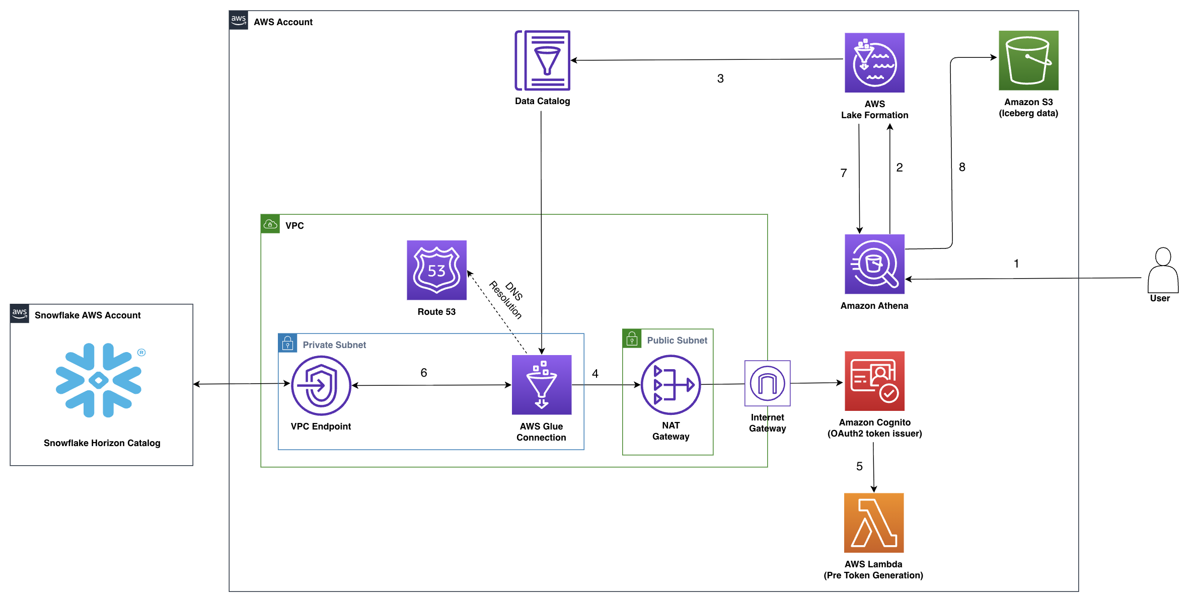
Query path from Amazon Athena through AWS Lake Formation and an AWS Glue connection to Snowflake and Amazon S3

Figure 1: Architecture for Snowflake Horizon Catalog federation to AWS Lake Formation using Amazon Cognito

Here’s how the workflow runs:

  1. A user or application submits a SQL query in Amazon Athena that references a federated table in the Snowflake catalog.
  2. Athena delegates catalog resolution and permission checks to Lake Formation, which evaluates fine-grained access controls on the federated catalog entry.
  3. Lake Formation resolves the table reference through the AWS Glue Data Catalog, which holds the connection configuration for Snowflake and invokes the AWS Glue connection.
  4. AWS Glue connection runs in a private subnet. It sends a client_credentials request to the Amazon Cognito token endpoint with the client ID, client secret, and scope. The request leaves through the NAT gateway and internet gateway because the machine-to-machine token endpoint is public.
  5. Amazon Cognito invokes the Pre Token Generation Lambda trigger (V3_0), which adds the aud claim that Snowflake External OAuth validation requires. Amazon Cognito returns the access token to the connection.
  6. Using that token, AWS Glue connection calls the Snowflake Horizon Catalog Iceberg REST endpoint for table metadata. The response includes the schema and the location of the data files in Amazon S3. An Amazon Route 53 private hosted zone resolves the hostname, because the Snowflake endpoint service doesn’t provide private DNS. The request travels through the VPC endpoint over AWS PrivateLink.
  7. The connection returns the metadata to Lake Formation, which generates temporary, scoped Amazon S3 credentials and passes them to Athena.
  8. Athena uses those credentials to read the Iceberg metadata and Parquet data files from the registered Amazon S3 location, runs the query, and returns results.

Why Amazon Cognito

AWS Glue connection authenticates with the OAuth2 client_credentials grant, so providers Snowflake trusts that support that grant can issue the token. Samsung Ads chose Amazon Cognito for three reasons:

  • Each table lookup against Snowflake depends on a token from the provider, so the team wanted to own it alongside the rest of the solution.
  • An enterprise identity provider is typically administered by a central security team, so each new machine-to-machine client is a cross-team request. Owning the user pool makes it self-service.
  • Each app client is a distinct machine identity, and the security integration trusts the user pool rather than an individual client. You can therefore serve several workloads from one integration, each with its own read-only Snowflake role.

Prerequisites

Before you begin, verify that you have the following:

  • Snowflake account hosted on AWS in the same AWS Region where you create the AWS resources in this post, on the Business-Critical edition or higher, which AWS PrivateLink requires. Confirm the Region with SELECT CURRENT_REGION();. You need ACCOUNTADMIN to create the security integration and to authorize PrivateLink.
    • Snowflake-managed Iceberg tables created in Snowflake Horizon Catalog using CATALOG = 'SNOWFLAKE' with an external volume pointing to the S3 bucket. If you don’t have one, see Configure an external volume for Amazon S3 in the Snowflake documentation.
  • AWS account with an AWS Identity and Access Management (IAM) principal that has data lake administrator permissions in AWS Lake Formation. The principal also needs permissions to create IAM roles and policies, Amazon Cognito user pools, AWS Lambda functions, VPC resources, and AWS CloudShell. We use AWS Command Line Interface (AWS CLI) commands throughout this post.
  • Amazon S3 bucket that holds your Snowflake-managed Iceberg data files.
  • An AWS user with long-term access keys that you delete immediately after Step 4:
    • SYSTEM$AUTHORIZE_PRIVATELINK needs a federation token from the long-term keys of an IAM user, because sts:GetFederationToken rejects role-session credentials. Snowflake persists the authorization, so you can delete the key and the user afterwards and the federation keeps working.

Walkthrough

Two AWS CloudFormation stacks cover the setup that is identical in every deployment. The Snowflake and Lake Formation steps stay as explicit SQL and AWS CLI commands, so you can adapt them to your existing Snowflake account and VPC.

Step What you configure How you run it
1 & 2 Cognito user pool, machine-to-machine app client, and the Lambda function that adds the aud claim Launch Stack, snowflake-federation-oauth
3 Snowflake security integration, read-only role, service user, and table grants Snowflake SQL worksheet
4 PrivateLink authorization for your AWS account AWS CLI and Snowflake SQL worksheet
5 VPC, PrivateLink endpoint, Route 53 private hosted zone, and the Lake Formation data access role Launch Stack, snowflake-federation-network
6 S3 location registration, AWS Glue connection, federated catalog, and Lake Formation permissions AWS CLI
7 Query validation Athena console

Step 1: Deploy the Cognito user pool and token customization Lambda function

Snowflake External OAuth validation requires an aud claim in each access token. The OAuth2 client_credentials grant doesn’t define that claim, so the Pre Token Generation trigger adds it. This stack creates the user pool, the machine-to-machine app client, and a Pre Token Generation Lambda function that adds the claim. The stack also writes the app client secret to AWS Secrets Manager in the format the AWS Glue connection expects. It then generates the Snowflake SQL statements you run in Step 3.

  1. Choose Launch Stack.

Launch Stack

  1. In the Region selector, confirm the Region matches your Snowflake account Region, then choose Next.
  2. For Stack name, keep snowflake-federation-oauth. Leave all parameters at their default values, then choose Next.
  3. On Configure stack options, keep the defaults and choose Next.
  4. On Review and create, select I acknowledge that AWS CloudFormation might create IAM resources with custom names, then choose Submit.
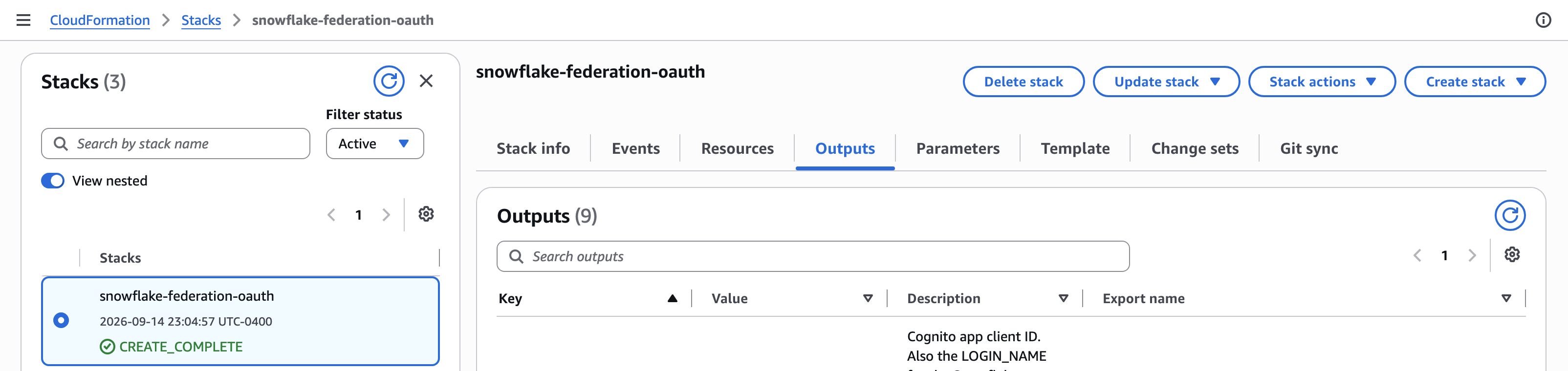
  5. When the stack status is CREATE_COMPLETE, choose the Outputs tab.

You use six of the outputs in later steps.

Output Used in
VerifyAudClaimCommand Step 2
SnowflakeSecurityIntegrationSQL Step 3
OAuthClientSecretArn Step 5 and Step 6
CognitoTokenEndpoint, CognitoClientId and CognitoScope Step 3 and Step 6
CloudFormation Outputs tab listing the six stack outputs used in later steps

Figure 2: CloudFormation Outputs tab showing the values used in later steps

Note: After the connection validates in Step 6, AWS Glue caches the token it mints by writing it back into this secret. Treat read access to the secret as read access to the federated tables.

Step 2: Verify the access token

Confirm that the Lambda function is adding the claim before you configure Snowflake. A missing claim doesn’t fail here. It surfaces several steps later as an AWS Glue connection that can’t authenticate, which is harder to attribute.

  1. On the Outputs tab, copy the value of VerifyAudClaimCommand.
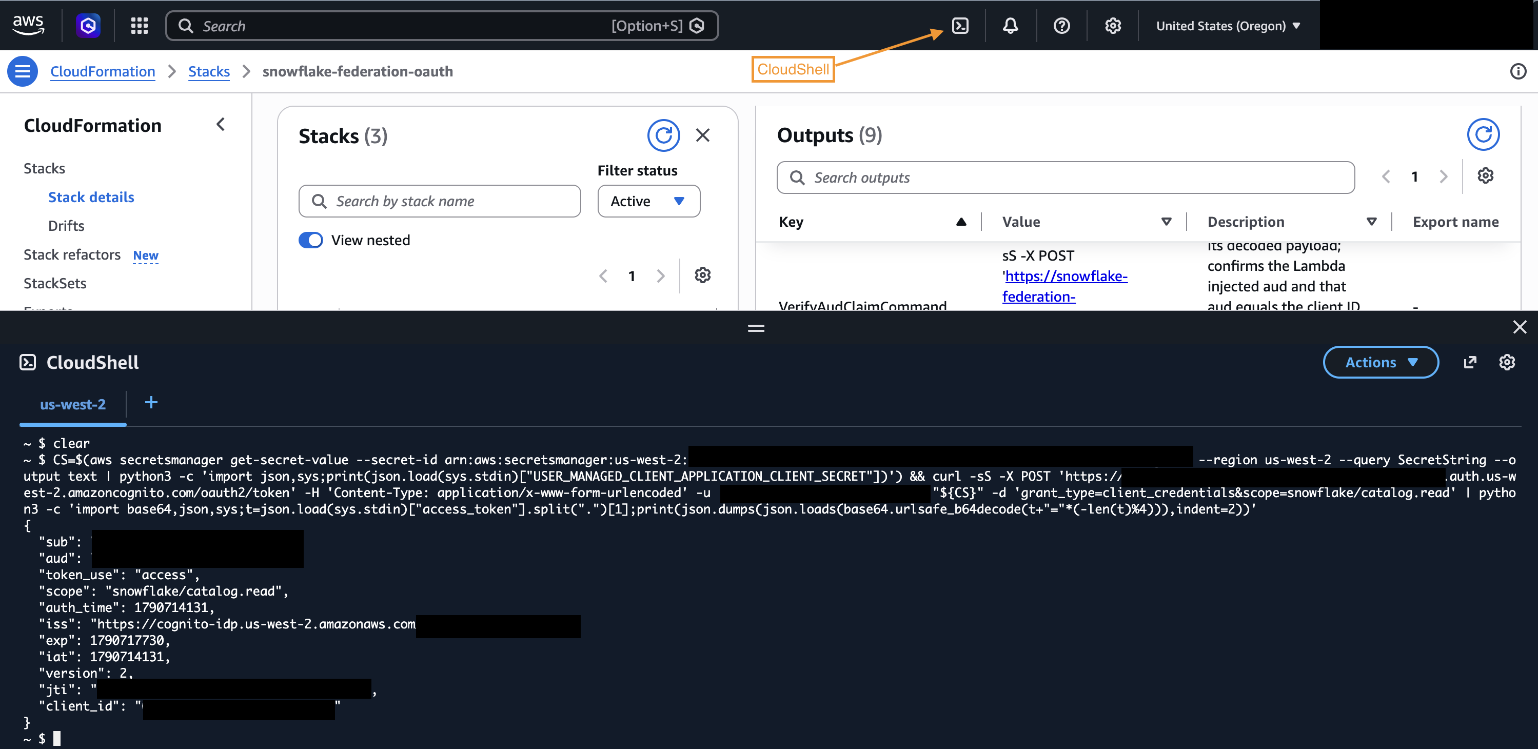
  2. Choose the AWS CloudShell icon on the console navigation bar, as shown in the following screenshot.
  3. Paste the command and run it. Confirm two values in the output. The aud claim matches your Cognito client ID, and scope is snowflake/catalog.read.
Decoded access token payload showing the injected aud claim and the snowflake/catalog.read scope

Figure 3: Decoded access token payload showing the injected aud claim and the catalog.read scope

Step 3: Configure Snowflake

In this step you configure Snowflake to trust Cognito tokens, create the service user that Lake Formation authenticates as, and grant it read access to your tables.

  1. Run the following statement in a Snowflake worksheet, replacing the three placeholders with the CognitoIssuerUri, CognitoJwksUrl, and CognitoClientId outputs from Step 1. The SnowflakeSecurityIntegrationSQL output contains the same statement with your values filled in. CREATE omits OR REPLACE, so it fails rather than overwriting an existing integration.
USE ROLE ACCOUNTADMIN;

-- Return a row if the integration exists. If so, use ALTER SECURITY INTEGRATION instead of CREATE
SHOW INTEGRATIONS LIKE 'lakeformation_cognito_oauth';

CREATE SECURITY INTEGRATION lakeformation_cognito_oauth
  TYPE = EXTERNAL_OAUTH
  ENABLED = TRUE
  EXTERNAL_OAUTH_TYPE = CUSTOM
  EXTERNAL_OAUTH_ISSUER = '<CognitoIssuerUri>'
  EXTERNAL_OAUTH_JWS_KEYS_URL = '<CognitoJwksUrl>'
  EXTERNAL_OAUTH_TOKEN_USER_MAPPING_CLAIM = 'sub'
  EXTERNAL_OAUTH_SNOWFLAKE_USER_MAPPING_ATTRIBUTE = 'login_name'
  EXTERNAL_OAUTH_AUDIENCE_LIST = ('<CognitoClientId>')
  EXTERNAL_OAUTH_ANY_ROLE_MODE = 'ENABLE'
  EXTERNAL_OAUTH_BLOCKED_ROLES_LIST = ('ACCOUNTADMIN', 'SECURITYADMIN', 'USERADMIN', 'SYSADMIN');

Snowflake normally takes the role from a session:role:<ROLE> scope, which Amazon Cognito custom scopes can’t carry because they use the form resourceServer/scope. The statement therefore sets EXTERNAL_OAUTH_ANY_ROLE_MODE to ENABLE, which lets the session use any role granted to the service user, so keep that user to a single role. The blocked roles list also covers SYSADMIN and USERADMIN, which the Snowflake default list doesn’t.

  1. Create the read-only role and the service user. Set LOGIN_NAME to the CognitoClientId output, because the token’s sub claim carries the client ID and the integration maps sub to login_name.
CREATE ROLE lakeformation_catalog_reader
  COMMENT = 'Read-only access for AWS Lake Formation catalog federation';

CREATE USER lakeformation_service_user_cognito
  LOGIN_NAME = '<CognitoClientId from Step 1>'
  DEFAULT_ROLE = lakeformation_catalog_reader
  TYPE = SERVICE;

GRANT ROLE lakeformation_catalog_reader TO USER lakeformation_service_user_cognito;
  1. Grant the role read access to the tables you want to federate. For the privileges the Iceberg REST Catalog API requires, see Configure access control in the Snowflake documentation.
GRANT USAGE ON DATABASE <database>
  TO ROLE lakeformation_catalog_reader;

GRANT USAGE ON SCHEMA <database>.<schema>
  TO ROLE lakeformation_catalog_reader;

GRANT SELECT ON ALL ICEBERG TABLES IN SCHEMA <database>.<schema>
  TO ROLE lakeformation_catalog_reader;

GRANT SELECT ON FUTURE ICEBERG TABLES IN SCHEMA <database>.<schema>
  TO ROLE lakeformation_catalog_reader;

Note: Federate a schema that contains only Snowflake-managed Iceberg tables. An externally managed table can fail the entire table listing. Converted tables, tables loaded from Iceberg-compatible Parquet files and clones whose source table the role can’t access aren’t supported. Tables with mixed-case quoted names aren’t federated, because the connection you create in Step 6 sets CATALOG_CASING_FILTER to UPPERCASE_ONLY.

Snowflake masking and row access policies don’t apply when Athena reads a federated table, because Lake Formation vends the Amazon S3 credentials and Athena reads the Parquet files directly. Keep tables that rely on them out of the federated schema or recreate the controls in Lake Formation and test them.

  1. Next, find the Amazon S3 bucket and prefix your external volume writes to. You need both in Step 5.
DESC EXTERNAL VOLUME <your_external_volume>;

STORAGE_BASE_URL holds the bucket and an optional prefix. For s3://my-bucket/iceberg/, the bucket is my-bucket and the prefix is iceberg. If nothing follows the bucket name, leave the prefix blank in Step 5. A prefix is better, because it limits the data access role to that path. If ENCRYPTION_TYPE is AWS_SSE_KMS, note the key in ENCRYPTION_KMS_KEY_ID for Step 5. If it is NONE, check the bucket’s default encryption in the Amazon S3 console. The Snowflake role that owns the Iceberg tables must keep the USAGE privilege on the external volume, or operations that request vended credentials fail.

If the bucket uses a customer managed KMS key, set KMS_KEY_ID on the external volume to the full key ARN. Then add the following statement to the key policy, so the session Snowflake uses for the role in STORAGE_AWS_ROLE_ARN can read the encrypted files. Without it, the AWS Glue connection fails with an error that says no session policy allows kms:Decrypt.

{
  "Sid": "AllowSnowflakeVolumeSession",
  "Effect": "Allow",
  "Principal": {
    "AWS": "arn:aws:sts::<account-id>:assumed-role/<external-volume-role>/snowflake"
  },
  "Action": [
    "kms:Decrypt",
    "kms:DescribeKey",
    "kms:GenerateDataKey"
  ],
  "Resource": "*"
}

Snowflake requires proof that you own the AWS account before it accepts a PrivateLink connection. You provide that proof as an AWS Security Token Service (AWS STS) federation token. You must call get-federation-token with the long-term credentials of an IAM user, because AWS STS doesn’t support calling it with temporary credentials from an assumed role.

  1. Using an IAM user with long-term access keys, generate a federation token:
aws sts get-federation-token --name snowflake-privatelink --duration-seconds 900 --profile <iam-user-profile>

The token appears in the SQL statement, so Snowflake keeps it in query history. The 15-minute duration limits how long it stays valid.

  1. In your Snowflake worksheet, pass your AWS account ID and the full JSON output from the previous command:
USE ROLE ACCOUNTADMIN;
SELECT SYSTEM$AUTHORIZE_PRIVATELINK('<aws-account-id>', '<full-federation-token-json>');

The output confirms that Snowflake authorized PrivateLink for your account.

Snowflake worksheet output confirming PrivateLink authorization for the AWS account

Figure 4: Snowflake output confirming PrivateLink authorization

  1. Retrieve the two values you need for the stack in Step 5:
WITH cfg AS (SELECT PARSE_JSON(SYSTEM$GET_PRIVATELINK_CONFIG()) AS j)
SELECT j:"regionless-privatelink-account-url"::string AS privatelink_hostname,
       j:"privatelink-vpce-id"::string AS vpce_service_name
FROM cfg;

Record both values. privatelink_hostname is the Snowflake PrivateLink hostname, and vpce_service_name is the endpoint service name.

After authorization succeeds, delete the temporary IAM user and its access key. Revoking PrivateLink access later requires a new federation token, so recreate a similar user at that point. For more information, see How to retrieve a Federation Token from AWS for PrivateLink Self-Service.

This stack creates the interface VPC endpoint to the Snowflake PrivateLink service and the Amazon Route 53 private hosted zone that resolves your Snowflake hostname to it. It also creates the security group that the endpoint shares with the AWS Glue connection. Keep Existing VPC ID blank and it also builds a VPC with public and private subnets and a NAT gateway.

To use an existing VPC, supply Existing VPC ID and two or more private subnet IDs in different Availability Zones. The stack then creates no subnets and no NAT gateway, so confirm three things first:

  • You have enabled DNS resolution and DNS hostnames on the VPC.
  • The private subnets have a 0.0.0.0/0 route to a NAT gateway, which the AWS Glue connection uses to reach the Amazon Cognito token endpoint. Amazon Cognito doesn’t support AWS PrivateLink, but the traffic stays on the AWS network because both sit in the same Region. Without this route, the stack still succeeds and the connection fails in Step 6.
  • No Amazon Route 53 private hosted zone for privatelink.snowflakecomputing.com is already associated with the VPC. A second zone for the same domain makes name resolution unpredictable.

To deploy the stack, complete the following steps:

  1. Choose Launch Stack.

Launch Stack

  1. Confirm the Region selector matches your Snowflake account Region, then choose Next.
  2. For Stack name, keep snowflake-federation-network, then enter the following parameters.
Parameter Value
Snowflake PrivateLink hostname privatelink_hostname from Step 4
Snowflake PrivateLink service name vpce_service_name from Step 4
Iceberg S3 bucket name The bucket in the STORAGE_BASE_URL output from Step 3
Iceberg data key prefix The prefix in the STORAGE_BASE_URL output from Step 3. Leave blank if you have none
Iceberg bucket KMS key ARN KMS key ARN. Leave blank if the bucket does’t use KMS
OAuth client secret ARN OAuthClientSecretArn from Step 1

If the bucket uses SSE-KMS, the stack grants the data access role kms:Decrypt on the key you enter. The default key policy already allows this. If your key policy doesn’t delegate access to IAM, add the role as a key user.

  1. Choose Next, keep the defaults on Configure stack options, and choose Next.
  2. On Review and create, select I acknowledge that AWS CloudFormation might create IAM resources with custom names, then choose Submit.
  3. When the stack status is CREATE_COMPLETE, which takes about 5 minutes, choose the Outputs tab and record PrivateSubnetIds, GlueConnectionSecurityGroupId, LakeFormationDataRoleArn, and RegisteredS3Location. You use all four values in Step 6.

NAT gateway and the interface VPC endpoint carry hourly and data processing charges. For more information, see Amazon VPC pricing.

Step 6: Register with Lake Formation and create the federated catalog

The remaining setup is a sequence of AWS CLI commands. Run them in AWS CloudShell in the same Region as both stacks.

  1. Set the values used by the commands that follow. Fill in the Region, and the stack outputs from Step 1 and Step 5.
REGION='<your Region>'
ACCT=$(aws sts get-caller-identity --query Account --output text)
PREFIX=snowflake-federation
CONN=$PREFIX-iceberg-connection
CATALOG=$PREFIX-catalog
S3_LOCATION='<RegisteredS3Location from Step 5>'
LFROLE='<LakeFormationDataRoleArn from Step 5>'
SECRET_ARN='<OAuthClientSecretArn from Step 1>'
TOKEN_URL='<CognitoTokenEndpoint from Step 1>'
CLIENT_ID='<CognitoClientId from Step 1>'
SCOPE='<CognitoScope from Step 1>'
SUBNET='<one subnet ID from PrivateSubnetIds in Step 5>'
SG='<GlueConnectionSecurityGroupId from Step 5>'
WORKSPACE_URL='https://<privatelink_hostname from Step 4>/polaris/api/catalog'
REMOTE_DB='<Snowflake database name, uppercase>'
SCHEMA='<Snowflake schema name, lowercase>'
QUERY_PRINCIPAL='<IAM role or user ARN that will run Athena queries>'
  1. Register the Amazon S3 location that holds your Iceberg data. This is what lets Lake Formation vend scoped credentials to Athena for the underlying data files.
aws lakeformation register-resource \
  --resource-arn "$S3_LOCATION" \
  --role-arn "$LFROLE" --with-federation
  1. Create the AWS Glue connection. This writes the definition to a file, then creates it.
cat > conn.json <<JSON
{
  "Name": "$CONN",
  "Description": "Snowflake Iceberg REST catalog through AWS Cognito.",
  "ConnectionType": "ICEBERGRESTCATALOG",
  "ConnectionProperties": {
    "INSTANCE_URL": "$WORKSPACE_URL",
    "ROLE_ARN": "$LFROLE",
    "CATALOG_CASING_FILTER": "UPPERCASE_ONLY"
  },
  "AuthenticationConfiguration": {
    "AuthenticationType": "OAUTH2",
    "SecretArn": "$SECRET_ARN",
    "OAuth2Properties": {
      "OAuth2GrantType": "CLIENT_CREDENTIALS",
      "TokenUrl": "$TOKEN_URL",
      "OAuth2ClientApplication": { "UserManagedClientApplicationClientId": "$CLIENT_ID" },
      "TokenUrlParametersMap": { "scope": "$SCOPE" }
    }
  },
  "PhysicalConnectionRequirements": {
    "SubnetId": "$SUBNET",
    "SecurityGroupIdList": ["$SG"]
  }
}
JSON

aws glue create-connection --connection-input file://conn.json
  1. Check the connection status. AWS Glue validates asynchronously. It creates the network interface, completes the OAuth2 exchange with Amazon Cognito, and calls the Snowflake Iceberg REST API over AWS PrivateLink. Repeat this command until it returns READY, which takes approximately 5–10 minutes.
aws glue get-connection --name $CONN --query Connection.Status --output text

If it returns FAILED, read the reason and correct the Snowflake configuration from Step 3. A missing security integration, service user, or grant is the usual cause.

aws glue get-connection --name $CONN --query Connection.StatusReason --output text

Then delete the connection before you retry, because the name stays in use.

aws glue delete-connection --connection-name $CONN
  1. Register the connection with Lake Formation using privileged access. A federated catalog can only use a connection registered this way.
aws lakeformation register-resource \
  --resource-arn arn:aws:glue:$REGION:$ACCT:connection/$CONN \
  --role-arn "$LFROLE" --with-federation --with-privileged-access
  1. Create the federated catalog, then confirm the tables surface through it.
aws glue create-catalog --name $CATALOG --catalog-input '{
  "FederatedCatalog": {"Identifier": "'"$REMOTE_DB"'", "ConnectionName": "'"$CONN"'"},
  "CreateDatabaseDefaultPermissions": [],
  "CreateTableDefaultPermissions": []
}'

aws glue get-tables --catalog-id $ACCT:$CATALOG --database-name $SCHEMA --query 'TableList[].Name'
  1. Grant Lake Formation permissions to the data teams that will query the tables. The principal that created the catalog can already query it. Every other principal needs an explicit grant, including other Lake Formation administrators.
aws lakeformation grant-permissions \
  --principal DataLakePrincipalIdentifier="$QUERY_PRINCIPAL" \
  --resource '{"Database":{"CatalogId":"'"$ACCT:$CATALOG"'","Name":"'"$SCHEMA"'"}}' \
  --permissions DESCRIBE

aws lakeformation grant-permissions \
  --principal DataLakePrincipalIdentifier="$QUERY_PRINCIPAL" \
  --resource '{"Table":{"CatalogId":"'"$ACCT:$CATALOG"'","DatabaseName":"'"$SCHEMA"'","TableWildcard":{}}}' \
  --permissions SELECT DESCRIBE

Note: The catalog ID for a federated catalog is :, not the bare account ID. Using the bare account ID grants permissions on the local AWS Glue Data Catalog instead, which succeeds and then leaves Athena returning an access denied error.

Step 7: Query the federated tables from Amazon Athena

  1. Open the Amazon Athena console and choose Query editor. If this is the first time you use Athena in this Region, choose Settings, then Manage, and set an Amazon S3 location for query results.
  2. In the left panel, select the following.
Field Value
Data source AwsDataCatalog
Catalog Your federated catalog, for example snowflake-federation-catalog
Database Your Snowflake schema name, in lowercase
  1. Run the following query:
SELECT * FROM "<snowflake_schema>"."<snowflake_tablename>" LIMIT 10;

Rows in the results pane confirm the federation works end to end, as shown in the following screenshot.
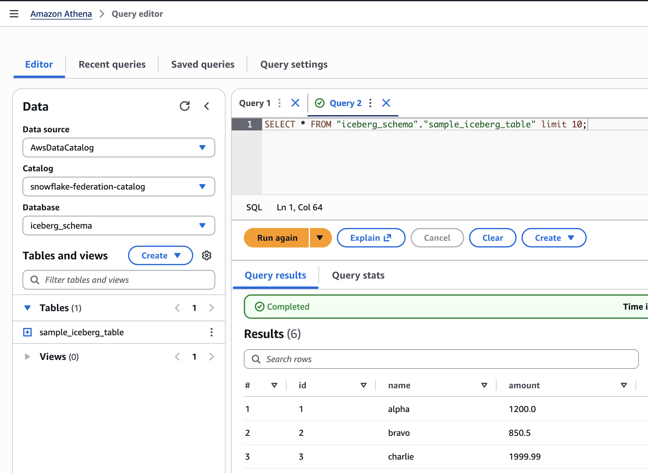
Amazon Athena query results returning 10 rows from a Snowflake-managed Iceberg table

Figure 5: Query results in Amazon Athena from a Snowflake-managed Iceberg table

To confirm that Athena reads current Snowflake data rather than a copy, insert a row in Snowflake and run the query again. The new row appears with no additional data movement into your AWS account.

Dropping a table in Snowflake doesn’t revoke the Lake Formation permissions granted on it. Revoke those permissions explicitly when you remove a federated table.

Clean up

To avoid incurring future charges, delete the resources you created while following this post. Complete the following steps in both your AWS account and your Snowflake account.

AWS account

  1. On the AWS Lake Formation console, choose Catalogs, select your federated catalog, then choose Actions and Delete catalog.
  2. Record the network interfaces the AWS Glue connection created, while the connection still exists. Filtering on the Step 5 security group and the ICEBERGRESTCATALOG description keeps the list to this deployment.
SG='<GlueConnectionSecurityGroupId from Step 5>'
aws ec2 describe-network-interfaces \
  --filters "Name=group-id,Values=$SG" "Name=description,Values=*ICEBERGRESTCATALOG" \
  --query 'NetworkInterfaces[].NetworkInterfaceId' --output text | tr '\t' '\n' > glue-enis.txt

cat glue-enis.txt
  1. Deregister and delete the AWS Glue connection. Do this before you delete the stacks, because the stack deletion fails while the connection’s network interfaces still hold the security group. Run the following in AWS CloudShell, replacing the Region, account ID, and connection name with your values.
aws lakeformation deregister-resource --resource-arn arn:aws:glue:<region>:<account-id>:connection/<glue-connection-name>
aws glue delete-connection --connection-name <glue-connection-name>
  1. Deleting the connection releases its network interfaces, but they stay in the in-use state for several minutes and AWS Glue doesn’t remove them. Wait for each one to reach available, because the Amazon Elastic Compute Cloud (Amazon EC2) console Detach action fails even with Force detachment selected. The following script checks each interface you recorded and deletes it when ready.
#!/bin/bash
while read -r eni; do
  [ -z "$eni" ] && continue
  for attempt in $(seq 1 20); do
    status=$(aws ec2 describe-network-interfaces \
      --network-interface-ids "$eni" \
      --query 'NetworkInterfaces[0].Status' \
      --output text 2>/dev/null || echo deleted)
    if [ "$status" = "available" ]; then
      aws ec2 delete-network-interface --network-interface-id "$eni"
      echo "$eni deleted"
      break
    fi
    if [ "$status" = "deleted" ]; then
      echo "$eni no longer exists"
      break
    fi
    echo "$eni is $status, checking again in 30 seconds"
    sleep 30
  done
done < glue-enis.txt
  1. On the Lake Formation console, under Administration, choose Data lake locations, select the registered Amazon S3 location, then choose Actions and Remove.
  1. On the AWS CloudFormation console, delete snowflake-federation-network first, then snowflake-federation-oauth. This removes the VPC endpoint, the Amazon Route 53 private hosted zone, the security group, and the IAM role. It also removes the Amazon Cognito user pool, the AWS Lambda function, and the client secret. If the stack created the VPC, subnets, and NAT gateway, it removes those too.

Snowflake account

  1. Open a SQL worksheet and run the following:
USE ROLE ACCOUNTADMIN;
DROP SECURITY INTEGRATION lakeformation_cognito_oauth;

USE ROLE USERADMIN;
DROP USER lakeformation_service_user_cognito;
DROP ROLE lakeformation_catalog_reader;
  1. Revoke the PrivateLink authorization for your AWS account. This requires a fresh federation token, generated the same way as during setup, from an IAM user with long-term access keys:
aws sts get-federation-token --name snowflake-privatelink --duration-seconds 900 --profile <iam-user-profile>
USE ROLE ACCOUNTADMIN;
SELECT SYSTEM$REVOKE_PRIVATELINK('<aws-account-id>', '<full-federation-token-json>');
  1. Confirm the account is no longer authorized:
SELECT SYSTEM$GET_PRIVATELINK_AUTHORIZED_ENDPOINTS();

Deleting the federated catalog and connection doesn’t delete data in Snowflake or Amazon S3. It only removes the federation configuration in your AWS account.

Conclusion

In this post, you learned how to federate Snowflake Horizon Catalog Iceberg tables into AWS Lake Formation and query them from Amazon Athena. Amazon Cognito handled the OAuth2 tokens for machine-to-machine authentication. To extend this pattern to additional workloads, create a new app client in your Cognito user pool and a corresponding read-only Snowflake role.

To get started, see Catalog federation to remote Iceberg catalogs and Federate to Snowflake Iceberg Catalog in the AWS Lake Formation Developer Guide, and External OAuth overview in the Snowflake documentation. If you have feedback about this post, submit comments in the Comments section.


About the authors

Ajay Gunasekaran

Ajay Gunasekaran

Ajay is an ML Platform Engineer at Samsung Ads. He has been instrumental in building the ML platform across the Snowflake and AWS ecosystems and is passionate about making complex infrastructure simple, reliable, and easy to use. Curious by nature, he enjoys learning, sharing ideas, and solving challenging problems.

Balaji Selva Rajan

Balaji Selva Rajan

Balaji is a Technical Account Manager at AWS, specializing in Cloud Operations, Storage, and Data Analytics. He helps customers to run their workloads efficiently on AWS and is particularly interested in turning recurring customer problems into repeatable, reusable patterns.

David Zhang

David Zhang

David is a Senior Specialist Solutions Architect specializing in Data & AI at AWS, where he focuses on designing and implementing open lakehouse architectures and agentic AI solutions. He is an active speaker at AWS events and contributes to technical publications and open-source initiatives. He is also the co-author of Apache Iceberg on AWS book. Outside of work, David enjoys staying active through volleyball, tennis, and basketball.

Steven Alyekhin

Steven Alyekhin

Steven is a Senior Solutions Architect on the AWS Canada ISV team, where he helps software companies build generative AI, machine learning, and data solutions on AWS.

Allocate shared Amazon MSK costs to Kafka topics for cost visibility

Post Syndicated from Durai Krishnan original https://aws.amazon.com/blogs/big-data/allocate-shared-amazon-msk-costs-to-kafka-topics-for-cost-visibility/

Your AWS bill shows Amazon Managed Streaming for Apache Kafka (Amazon MSK) charges at the cluster level, with one cost line item for each cluster. If your organization runs one cluster for several teams, and each team owns its own Kafka topics, you need a way to show each team its share of the spend. This post shows how you can produce that per-topic cost view by combining cluster-level billing data with per-topic usage metrics. The result gives each team a usage-based picture of what it consumes.

Bringing cost and usage together

You can use Amazon MSK to run Apache Kafka at scale while AWS manages the underlying infrastructure, so you can focus on configuring and operating your applications. Many organizations consolidate multiple workloads onto a single cluster, where each team or application owns a set of Kafka topics. Consolidation can help you improve operational efficiency. When you implement per-topic cost visibility, you can show each team its share of the cluster spend.

Producing that view draws on two sources of data, and the solution brings them together.

Cost: cluster-level billing in the CUR

You can locate MSK charges in your AWS Cost and Usage Report (CUR) by cluster ARN and see operations such as RunBroker, RunVolume, and Bandwidth. You use this cluster-level cost as the starting point when you allocate costs to your topics.

Usage: per-topic metrics without cost context

Amazon MSK surfaces per-topic throughput metrics, which provide the usage signal you use to distribute cluster cost across topics. You can use the cluster name that Amazon MSK provides with these metrics. Map that name to the cluster ARN to join usage with billing and produce per-topic cost.

Solution overview

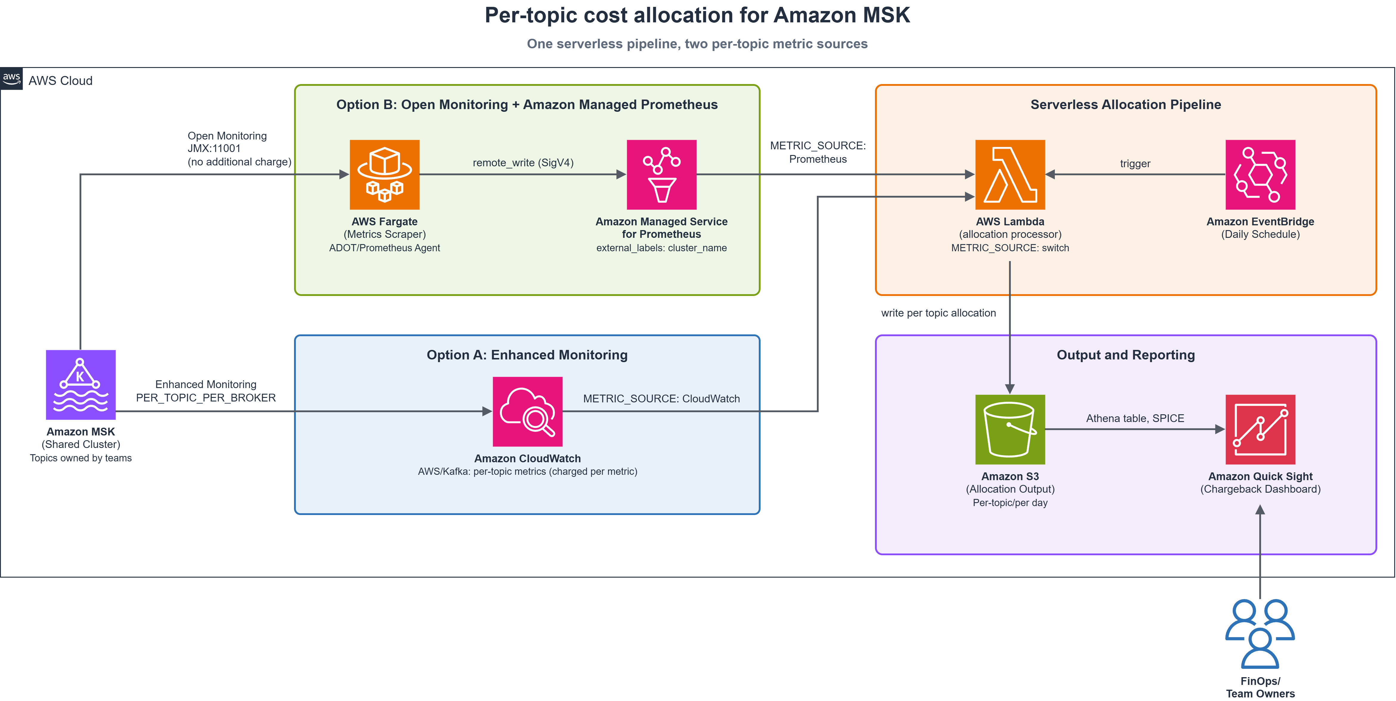
Option A – Enhanced Monitoring: Uses per-topic Amazon CloudWatch metrics published by Amazon MSK.

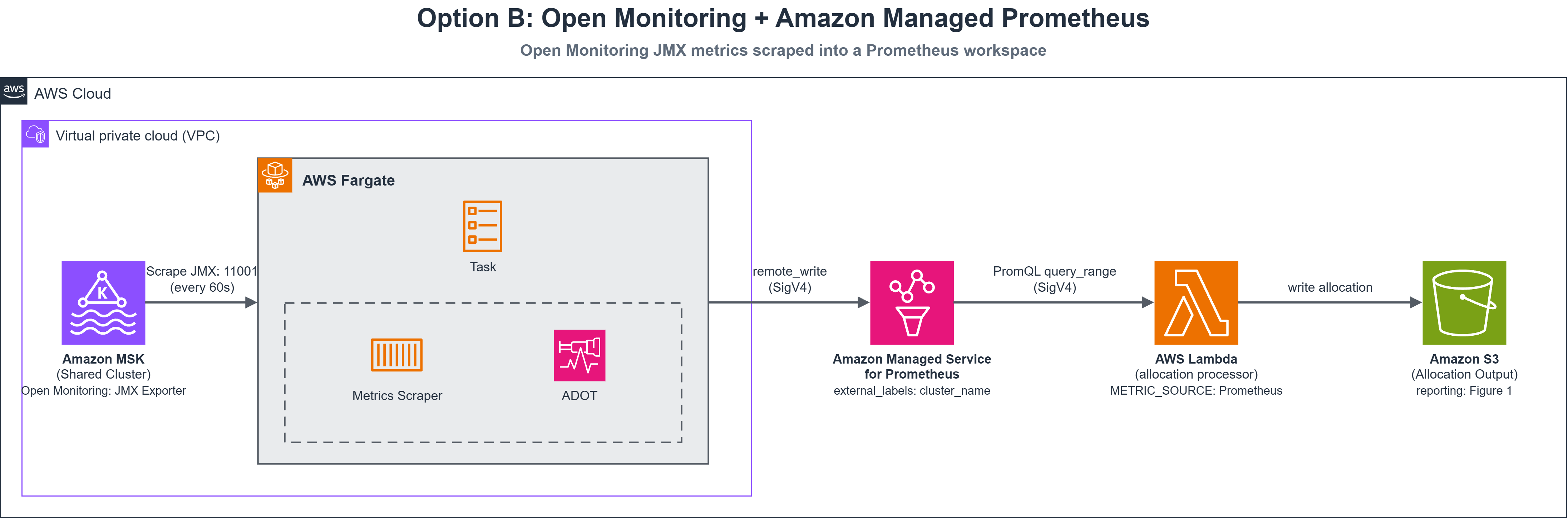
Option B – Open Monitoring with Amazon Managed Service for Prometheus: A cost-optimized alternative. This option uses the MSK Open Monitoring endpoint at no additional charge and keeps metric cost growth low as topic count grows.

Both options use the same allocation logic and output. Switch between them with one configuration value.

The pipeline runs in five steps:

  1. Read cluster cost from CUR – A daily AWS Lambda function reads MSK line items by cluster ARN and day.
  2. Bridge identifiers – The function calls ListClustersV2 to map cluster name to ARN.
  3. Read per-topic usage – The function retrieves each topic’s daily throughput. This step differs between Option A and Option B.
  4. Allocate proportionally – For each day, the function distributes that day’s cluster cost across topics based on each topic’s share of throughput.
  5. Publish results – The function writes allocation data as Apache Parquet to Amazon Simple Storage Service (Amazon S3) and refreshes an Amazon Athena table. You visualize the results in AWS Quick Sight.

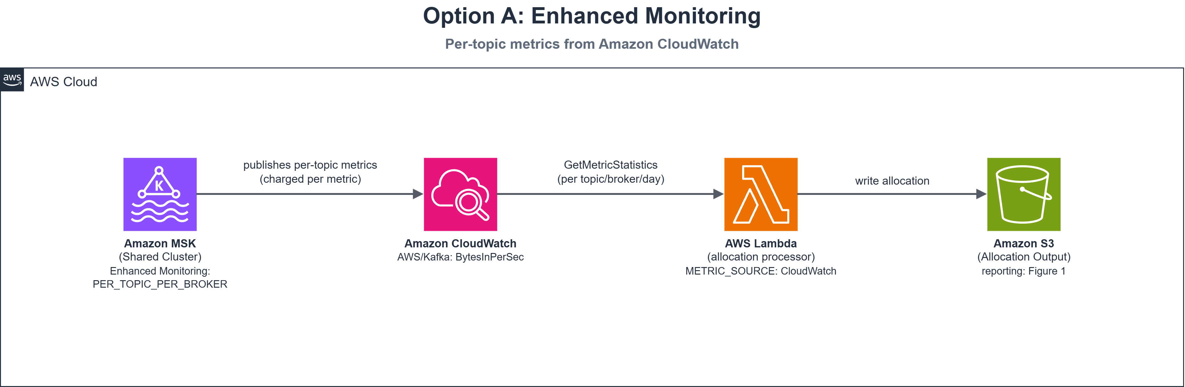
The following diagram shows the pipeline.

Serverless pipeline allocating MSK cluster cost to Kafka topics from CUR and per-topic metrics, output to Amazon S3 and Quick Sight

Figure 1: Solution architecture. A single serverless pipeline supports both per-topic metric sources, selected with the METRIC_SOURCE environment variable

How the allocation works

For each cluster and day, the function computes each topic’s share of ingress bytes and applies that share to the cost:

topic_run_cost = day_broker_cost × (topic_bytes / total_cluster_bytes)
topic_storage_cost = day_storage_cost × (topic_bytes / total_cluster_bytes)
topic_total_cost = topic_run_cost + topic_storage_cost

The function assigns 30 percent of the cost to a topic that carries 30 percent of ingress. Allocations always sum to the day’s total. During a partial outage, the function distributes costs only among topics for which you have configured metrics.

Two behaviors to know:

  • Idle topics get no row. If only 3 of 20 report traffic, those 3 absorb the full cost. The allocation_method column catches this.
  • If no topic reports traffic for a cluster-day, the function falls back to an even split across all topics you have configured.

Why bytes-in as the allocation weight

Bytes-in is available from both metric sources and correlates well with broker compute and network cost.

However, bytes-in is a proxy. Its limitations:

  • It can’t see retention. Two topics with identical throughput but different retention periods use different storage.
  • It can’t see replication factor or compression, which change actual bytes on disk.
  • It can’t see consumer fan-out. A topic read by ten consumer groups looks the same as one read by one.

Other factors can drive your costs, such as egress (consumer read volume), partition count, or storage retention. In that case, you can adapt the same pipeline to use a different allocation weight or a blended model.

Report unallocated charges (data transfer, tiered storage, MSK Connect) explicitly so finance has a more complete picture.

Prerequisites

Before you begin, make sure you have:

  • An active Amazon MSK Provisioned cluster with topics carrying traffic. (Amazon MSK Serverless is out of scope. It bills differently and does not expose per-topic BytesInPerSec.)
  • AWS CUR (or AWS Data Exports for CUR 2.0) delivering Parquet to Amazon S3 with resource IDs enabled. Uses CUR 2.0 snake_case column names.
  • An AWS Glue catalog table over the CUR data with correct partition configuration.
  • Permissions to create AWS Lambda functions, IAM roles, Athena tables, and Quick Sight resources.
  • Quick Sight Enterprise edition (for SPICE datasets and row-level security in the reporting layer).
  • For Option B only: a private subnet in the MSK virtual private cloud (VPC) for the scraper, and an Amazon Managed Service for Prometheus workspace.

Timing: CUR lags up to 24 hours. Per-topic metrics exist only from the moment you enable them.

Sourcing per-topic usage: Two options

How you collect per-topic usage is the main design decision in this solution, because it determines your monitoring cost and setup effort. The pipeline supports both options, and you select one with the METRIC_SOURCE environment variable.

When you set Enhanced Monitoring to PER_TOPIC_PER_BROKER, MSK publishes per-topic throughput metrics to CloudWatch. The Lambda function aggregates each topic’s daily usage with GetMetricStatistics calls.

Option A path: Amazon MSK publishes per-topic metrics to CloudWatch, which the allocation Lambda function reads directly

Figure 2: Option A collection path. Amazon MSK publishes per-topic metrics to CloudWatch, and the allocation function reads them directly

Code sample — reading per-topic metrics from CloudWatch:

result = cloudwatch.get_metric_statistics(
    Namespace='AWS/Kafka', MetricName='BytesInPerSec',
    Dimensions=[
        {'Name': 'Cluster Name', 'Value': cluster_name},
        {'Name': 'Broker ID', 'Value': str(broker_id)},
        {'Name': 'Topic', 'Value': topic},
    ],
    StartTime=day_start, EndTime=day_end,
    Period=86400, Statistics=['Sum'],
)

Note: BytesInPerSec is a rate. Period=86400 with Statistics=[Sum] returns a valid relative weight for proportional allocation, not total bytes.

Why start here: Nothing to deploy. Change one cluster setting and metrics appear in CloudWatch.

The trade-off: CloudWatch bills per metric. PER_TOPIC_PER_BROKER publishes a metric set for every topic-broker pair, so cost grows with both.

Scaling tip: At scale (over 50 clusters, over 200 topics), switch to GetMetricData (up to 500 metrics per call) instead of iterating GetMetricStatistics.

Option B (cost-optimized): Open Monitoring with Amazon Managed Service for Prometheus

Kafka brokers expose operational metrics through Java Management Extensions (JMX). Amazon MSK Open Monitoring makes these infrastructure metrics available in Prometheus format on port 11001 at no cost.

You run a scraper (AWS Fargate with an AWS Distro for OpenTelemetry (ADOT) Collector) that forwards metrics to a Prometheus workspace through SigV4 remote write. The task role needs the aps:RemoteWrite permission.

Option B path: a VPC scraper collects JMX metrics and remote-writes them to Amazon Managed Service for Prometheus

Figure 3: Option B collection path. A VPC scraper collects JMX metrics at no additional charge and forwards them to Prometheus

Scraper configuration (Prometheus agent):

global:
  scrape_interval: 60s
  external_labels:
    cluster_name: "<your-cluster-name>"  # allocation query filters on this

scrape_configs:
  - job_name: msk-jmx
    metrics_path: /metrics
    static_configs:
      - targets:
          - "b-1.<cluster>.<id>.kafka.<region>.amazonaws.com:11001"
          - "b-2.<cluster>.<id>.kafka.<region>.amazonaws.com:11001"

remote_write:
  - url: https://aps-workspaces.<region>.amazonaws.com/workspaces/<workspace-id>/api/v1/remote_write
    sigv4:
      region: <region>
      role_arn: arn:aws:iam::<central-account-id>:role/MskPromRemoteWriteRole
    queue_config:
      capacity: 2500
      max_samples_per_send: 1000

Get broker hostnames from GetBootstrapBrokers. For dynamic lists, use Prometheus file_sd_configs.

PromQL query for per-topic usage:

sum by (topic) (
  avg_over_time(
    kafka_server_BrokerTopicMetrics_OneMinuteRate_BytesInPerSec{cluster_name="<cluster>"}[1d]
  )
) * 86400

This averages broker rates over 24 hours into one value per topic, producing a comparable weight.

Open Monitoring is available at no additional charge and the Prometheus workspace bills on samples ingested, so metric cost grows slowly. This suits large fleets.

How the function discovers topics

The function resolves topic lists through a tiered lookup:

  1. Static topic map – An environment variable holding JSON keyed by cluster name. No API calls needed. Works well when you already track topic ownership in config or infrastructure code.
  2. Amazon MSK ListTopics API – Control-plane call, no VPC connectivity needed.
  3. CloudWatch ListMetrics – Reads topics from metric dimensions (Enhanced Monitoring only).
  4. Previous allocation output – Falls back to yesterday’s topic list from S3.

The tiered lookup keeps the function working whether or not Enhanced Monitoring is enabled:

def discover_topics(cluster_name, kafka_client=None, cluster_arn=None):
    """Resolve the topic list without requiring Enhanced Monitoring.
    Tiers are tried in order; the first that returns topics wins."""
    # Tier 1: static map from an env var (no API calls). Set TOPIC_LIST_JSON
    # to a JSON object keyed by cluster name, e.g. {"<cluster>": ["<topic>", ...]}
    if TOPIC_LIST_JSON:
        mapping = json.loads(TOPIC_LIST_JSON)
        if cluster_name in mapping:
            return set(mapping[cluster_name])
    # Tier 2: MSK ListTopics API - works at DEFAULT monitoring, no extra cost
    if kafka_client and cluster_arn:
        topics = _discover_topics_via_msk_api(kafka_client, cluster_arn)
        if topics:
            return topics
    # Tier 3: CloudWatch ListMetrics - only returns topics when Enhanced
    # Monitoring (PER_TOPIC_PER_BROKER) is enabled
    topics = _discover_topics_via_cloudwatch(cluster_name)
    if topics:
        return topics
    # Tier 4: fall back to the topic list from yesterday's allocation output in S3
    return _topics_from_previous_allocations()

Choosing between the options

For steady topics, both options typically produce comparable results. The choice is cost and operating model:

Option A: Enhanced Monitoring Option B: Open Monitoring + Prometheus
Per-topic metric cost ~$90/cluster/month None (Open Monitoring is at no additional charge)
Additional infra cost None ~$11/cluster/month (scraper + workspace)
Setup effort Change one cluster setting Deploy scraper, workspace, and VPC networking
Ongoing operations None Maintain one scraper per VPC
Scaling behavior Grows with topics × brokers Grows slowly from a much lower base
Time to first allocation Next day Next day (after a few days of setup)

Note: Figures are illustrative, not AWS list prices. Recalculate using the CloudWatch, Prometheus, and Fargate pricing pages.

Guideline: if monitoring cost is below 5 percent of MSK spend, take Option A. Above 10 percent, Option B repays the setup quickly.

You can enable Enhanced Monitoring only on clusters where chargeback accuracy matters, and switch to Option B later with one environment variable change.

Deploying the allocation pipeline

Deploy with AWS Cloud Development Kit (AWS CDK). The core Lambda function (Python 3.11, 1 GB, 10-min timeout) uses the AWS SDK for pandas layer for Parquet processing. Two triggers invoke the function, for resilience:

  • An Amazon S3 event notification fires when a new CUR Parquet file arrives, so allocation runs as soon as fresh cost data lands.
  • An Amazon EventBridge rule runs daily at 06:00 UTC as a fallback, in case the S3 event doesn’t arrive or CUR delivery lags.

Set METRIC_SOURCE to cloudwatch for Option A or prometheus for Option B. For Option B, you also supply the workspace query endpoint and label names.

The handler at a glance

The following handler function orchestrates the five-step pipeline. Each step delegates to a dedicated function, described in the sections that follow.

def handler(event, context):
    """Lambda entry point --- runs the five-step pipeline once per invocation."""
    # Step 1: read cluster cost from CUR (MSK rows only)
    daily_cur = read_cur_costs_via_athena()
    if not daily_cur:
        return _resp(200, 'No MSK costs found in CUR data')
    # Step 2: bridge identifiers - group cluster ARNs by account
    clusters_by_account = _group_clusters_by_account(daily_cur)
    # Steps 3-4: read per-topic usage and allocate cost proportionally, per cluster
    all_rows, errors = [], []
    for account_id, cluster_arns in clusters_by_account.items():
        try:
            all_rows.extend(process_account(account_id, cluster_arns, daily_cur))
        except Exception as e:
            errors.append({'account': account_id, 'error': str(e)})
    # Step 5: publish results - write Parquet to S3, refresh the Athena table
    write_allocations(all_rows)
    refresh_allocation_table()
    return _resp(200, {'rows_written': len(all_rows), 'errors': len(errors)})

CDK stack – Lambda function definition:

allocation_fn = lambda_.Function(
    self, "AllocationProcessor",
    runtime=lambda_.Runtime.PYTHON_3_11,
    handler="handler.handler",
    code=lambda_.Code.from_asset("src/lambda/allocation_processor"),
    timeout=Duration.minutes(10),
    memory_size=1024,
    dead_letter_queue=dlq,
    environment={
        "OUTPUT_BUCKET": allocation_bucket.bucket_name,
        "ATHENA_DATABASE": cur_database_name,
        "CUR_TABLE_NAME": cur_table_name,
        "ATHENA_OUTPUT": f"s3://{allocation_bucket.bucket_name}/athena-results/",
        # Option A. Switch to "prometheus" for Option B.
        "METRIC_SOURCE": "cloudwatch",
        # Option B only:
        # "AMP_QUERY_URL": "https://aps-workspaces.<region>.amazonaws.com/"
        # "workspaces/<workspace-id>/api/v1",
        # "AMP_CLUSTER_LABEL": "cluster_name",
        # "AMP_TOPIC_LABEL": "topic",
    },
    layers=[pandas_layer],
)

Triggers:

# Trigger 1: process when new CUR data arrives
cur_bucket.add_event_notification(
    s3.EventType.OBJECT_CREATED,
    s3n.LambdaDestination(allocation_fn),
    s3.NotificationKeyFilter(prefix="cur-clean/", suffix=".parquet"),
)

# Trigger 2: daily schedule as fallback
daily_rule = events.Rule(
    self, "DailyAllocationRule",
    schedule=events.Schedule.cron(hour="6", minute="0"),
)
daily_rule.add_target(targets.LambdaFunction(allocation_fn))

The stack provisions an Amazon Simple Queue Service (Amazon SQS) dead-letter queue with 14-day retention for failed invocations, Amazon Simple Notification Service (Amazon SNS) alerts, and CloudWatch alarms. To subscribe your team, add sns.Topic.add_subscription(subscriptions.EmailSubscription("[email protected]")) in CDK, or subscribe manually through the Amazon SNS console.

The stack creates the AWS Glue table over the allocation output, so you don’t need to write DDL by hand. Deploy it with:

cdk bootstrap  # once per account and Region
cdk deploy

Invoke the function once manually to produce a first allocation.

Reading CUR efficiently at scale

The function queries CUR through Amazon Athena to get only MSK rows. Filter on partition columns so Athena prunes whole partitions:

SELECT line_item_resource_id, line_item_usage_start_date,
       line_item_unblended_cost, line_item_operation
FROM "<cur_database>"."<cur_table>"
WHERE billing_period IN ('<current_month>', '<previous_month>')
  AND line_item_product_code = 'AmazonMSK'
  AND line_item_resource_id LIKE 'arn:aws:kafka:%'
  AND line_item_usage_start_date >= TIMESTAMP '<start_of_prev_month>'
  AND line_item_unblended_cost != 0

The query reads two months because AWS can update CUR line items after the first delivery. Adjust arn:aws:kafka: for GovCloud or the China Regions.

Publishing and querying the results

The function writes allocation results to Amazon S3 as Snappy-compressed Parquet, partitioned by billing period. Each row covers one topic on one day with cluster identity, usage weight, and allocated cost.

Each run overwrites the file for its billing period. This helps prevent double-counting on CUR redeliveries.

Output schema:

Field Description
account_id AWS account that owns the cluster
cluster_name, cluster_arn MSK cluster identity and join key back to the CUR
topic_name Kafka topic
client_id Owning team or client (from a configurable mapping)
allocation_date, year, month The day this row covers, plus year and month for convenient filtering
bytes_in Topic ingress used as the allocation weight
run_cost, storage_cost, total_cost Allocated cost components
**cluster_*_cost_day** Cluster totals for that day (for reconciliation against the bill)
allocation_method “proportional” or “equal_split” – explains anomalies without re-running
generated_at Timestamp of the run that produced this row

Verifying the numbers

Run this reconciliation query before publishing a dashboard. Schedule it as a Lambda post-step with an AllocationVariance CloudWatch alarm:

SELECT allocation_date,
       cluster_name,
       SUM(total_cost) AS allocated,
       MAX(cluster_run_cost_day + cluster_storage_cost_day) AS billed,
       SUM(total_cost) - MAX(cluster_run_cost_day + cluster_storage_cost_day) AS variance,
       MAX(allocation_method) AS method,
       COUNT(*) AS topics_charged
FROM topic_cost_allocation
WHERE billing_period = '<YYYY-MM>'
GROUP BY allocation_date, cluster_name
HAVING ABS(SUM(total_cost)
    - MAX(cluster_run_cost_day + cluster_storage_cost_day)) > 0.01
ORDER BY allocation_date;

An empty result means allocations reconcile. Rows indicate days where topic discovery and cost data disagreed.

Mapping topics to teams

The function derives owners from topic naming conventions. Pass an explicit topic-to-team map where conventions fail. Unmapped topics appear as unfamiliar owners.

Visualizing cost by topic in Quick Sight

Create an Athena data source in Quick Sight, import into SPICE, and schedule daily refreshes.

A useful dashboard typically includes:

  • A detail table of cost by team, topic, and month.
  • A bar chart of total cost by topic.
  • Filter controls for cluster, topic, and time period.

Apply Quick Sight row-level security against client_id so teams see only their own numbers. Row-level security requires Enterprise edition.

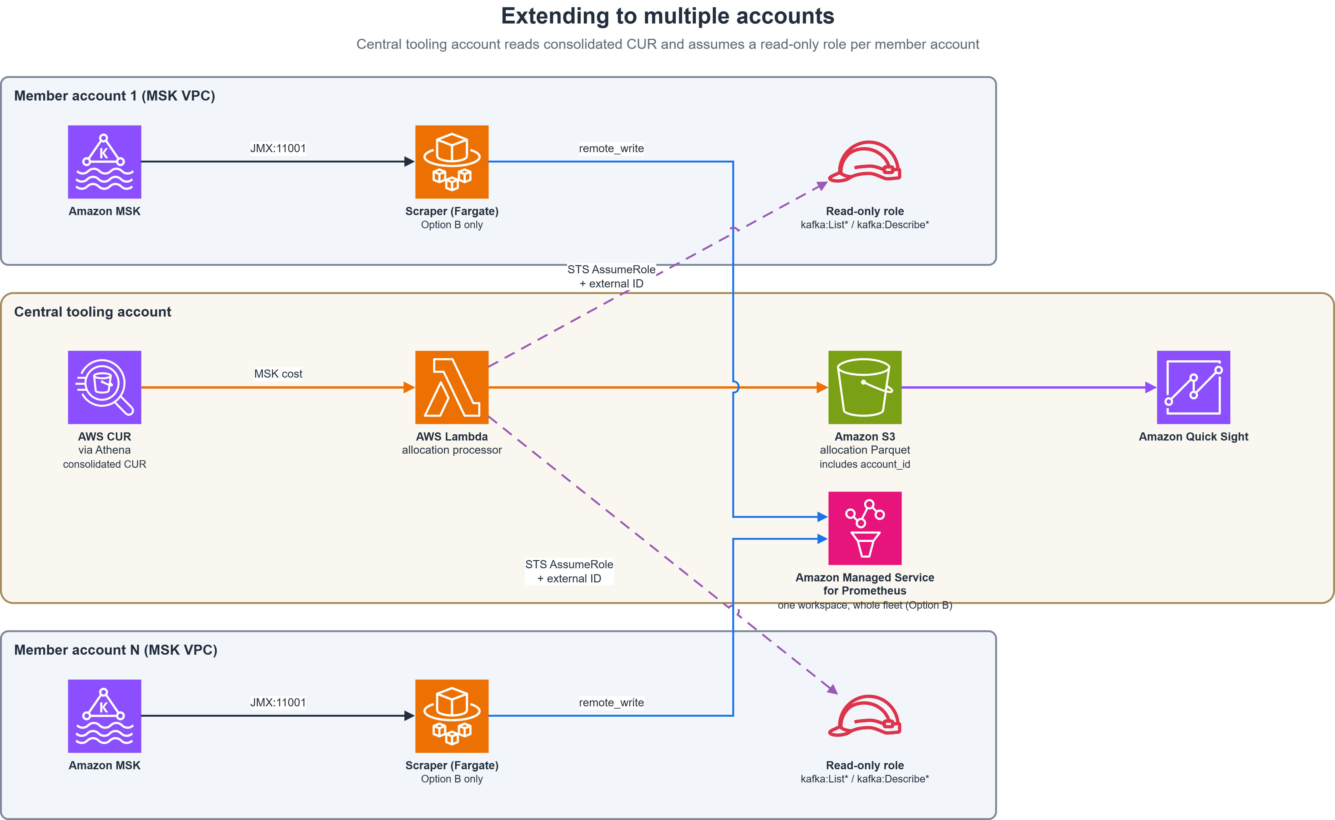
Extending to multiple accounts

The pipeline extends to multi-account setups:

  • The central account reads the consolidated CUR.
  • The Lambda function assumes a read-only role in each member account (by using AWS Security Token Service (AWS STS)) to list clusters and read usage, writing one consolidated dataset.
  • For Option B, a single central Prometheus workspace receives remote-writes from every member account’s scraper, each stamping its own cluster_name label.

One dataset and one dashboard across all accounts.

Multi-account setup: a central tooling account runs the pipeline and assumes read-only roles in member accounts

Figure 4: Multi-account extension. The central tooling account owns the pipeline and reaches into member accounts through a scoped, read-only role

Security considerations

This pipeline reads billing data and crosses account boundaries.

Grant the central execution role only the permissions it needs to: read the CUR and Glue catalog, run Athena queries, write to the allocation S3 bucket, and assume member-account roles.

Member-account role is read-only. Require a shared external ID on every AssumeRole call to help mitigate the confused-deputy problem.

For Option B, restrict port 11001 to the scraper’s security group. Consider AWS PrivateLink for remote write.

Encrypt CUR, allocation output, and Athena results at rest using SSE-KMS (recommended for financial data). Use TLS to encrypt data in transit, including the scraper’s remote write and Athena connections.

The output reveals what every team spends. Treat the output bucket and Quick Sight dataset as financial reports.

Cost of running the solution

The pipeline itself is inexpensive (Lambda, Athena, S3, Amazon EventBridge are negligible). Two items dominate:

  • The metric source: ~$90 (Option A) compared to ~$11 (Option B) per month on the example cluster.
  • Quick Sight user licenses: frequently the largest cost, scaling with how many people get access.

Clean up

To avoid ongoing charges, remove the resources you created. Delete Athena query result files and the CUR delivery configuration if created solely for this solution.

cdk destroy

If you enabled Enhanced Monitoring solely for this solution, return to the previous level. For Option B, remove the scraper and Prometheus workspace.

Conclusion

This pipeline bridges cluster-level CUR cost to topic-level usage, giving each team visibility into its share of the spend. Switch between monitoring options with one environment variable. Pick a cluster and run the allocation to get started.

Learn more:


About the authors

Durai Krishnan

Durai Krishnan

Durai is a Senior Customer Solution Manager at Amazon Web Services (AWS) with rich background in consulting and leadership. Durai specializes in guiding customers through their cloud journey, focusing on migration, modernization, and cost optimization strategies.

Ganesh Thiyagarajan

Ganesh Thiyagarajan

Ganesh is a Senior Solutions Architect at Amazon Web Services (AWS) with over 20 years of experience in software architecture, IT consulting, and solution delivery. He helps ISVs transform and modernize their applications on AWS. He is also part of the AI/ML Technical field community, helping customers build and scale Gen AI solutions.

Test your applications against AWS locally with AWS Emulator

Post Syndicated from Daniel Abib original https://aws.amazon.com/blogs/aws/test-your-applications-against-aws-locally-with-aws-emulator/

Today we’re announcing AWS Emulator, a local emulator for Amazon Web Services (AWS) that you run on your machine. The AWS Command Line Interface (AWS CLI), the AWS SDKs, and your coding agents speak to it over a local HTTPS endpoint using the same AWS APIs they would use in the cloud, from your laptop. AWS Emulator has no additional service fee. You pay only for AWS resources when you deploy on AWS. Its source is on GitHub. You install it from an RPM or Debian package on Linux, and on macOS and Windows you run it in Docker.

How it works
You install the emulator, start it, and point your tools at the local endpoint. When AWS Emulator starts, it generates its own credentials, a config file, and a certificate, and writes them to ~/.aws/emulator/9297/. You set environment variables so the AWS SDK talks to your laptop instead of AWS, and your application code stays unchanged.

From there, your existing tests, CLI scripts, and coding agents keep working the way they already do. A unit test that creates an Amazon DynamoDB table, writes an item, and reads it back is the same test, and it runs on your machine without a deployment. A coding agent can create resources, check the result, and iterate again without waiting on a deployment in a Region.

The emulator is implemented in Rust so that it stays light on CPU and memory on a laptop. It supports the APIs of AWS services that have an API model in the AWS API models repository on GitHub, and because it’s built from those models, the same ones the AWS SDKs use, your requests and the errors you get back have the same shape as on AWS.

If you are a developer, especially one working with coding agents such as Kiro or Claude Code, you can use that loop to test AWS interactions of real complexity locally.

Let’s try it out
To get started, I installed the package on Amazon Linux 2023. The package adds the aws-emulator command to /usr/bin/, so it’s on the path.

PKG=https://downloads.aws.com/aws-emulator/packages/aws-emulator/LTS/latest
sudo dnf install -y $PKG/aws-emulator-x86_64.rpm

aws-emulator -v

On macOS and Windows, you build a Docker image from the short Dockerfile in the documentation and run the emulator in a container. We don’t publish a ready-made image.

I started the emulator with aws-emulator. It serves HTTPS on 127.0.0.1:9297, so only my own computer can reach it, and it writes its log as JSON lines that show the address, the config file, and the certificate file.

aws-emulator

In another terminal, I set the environment variables that point the AWS CLI at the emulator, and unset any variables that could supply real AWS credentials.

export AWS_ENDPOINT_URL=https://127.0.0.1:9297
export AWS_SHARED_CREDENTIALS_FILE=~/.aws/emulator/9297/emulator_credentials
export AWS_CONFIG_FILE=~/.aws/emulator/9297/config
export AWS_EC2_METADATA_DISABLED=true
export AWS_DISABLE_HOST_PREFIX_INJECTION=true
export AWS_REGION=us-east-1
export AWS_DEFAULT_REGION=us-east-1
unset AWS_ACCESS_KEY_ID AWS_SECRET_ACCESS_KEY AWS_SESSION_TOKEN AWS_PROFILE

The emulator generates new keys each time it starts. Its access key IDs start with EMULATOR, so you can’t mistake them for real AWS keys, and it rejects requests signed with any other keys. To confirm that my shell was talking to the emulator, I checked the health endpoint and the caller identity. The emulator uses a single account, 000000000000.

curl --cacert ~/.aws/emulator/9297/ca.pem https://127.0.0.1:9297/__admin/health

aws sts get-caller-identity

Then I created a bucket, copied in a small object, and listed it.

$ aws s3 mb s3://local-getting-started
make_bucket: local-getting-started

$ echo "hello from the emulator" > hello.txt

$ aws s3 cp hello.txt s3://local-getting-started/
upload: ./hello.txt to s3://local-getting-started/hello.txt

$ aws s3 ls s3://local-getting-started/

With the AWS CLI pointed at my laptop, I had the same commands I already use and a local endpoint that answered them.

Next I wanted to see it the way I actually work now, so with the emulator still running I opened Kiro and asked it to create an Amazon DynamoDB table, write an item, and read it back, all against AWS Emulator rather than my AWS account.

kiro> Using the local AWS Emulator (the environment variables
      are already set in this shell), create a DynamoDB table
      "kiro-demo" with a string key "id", put an item
      {id: "item-1", msg: "hello from kiro"}, then read it
      back with get-item.

$ aws dynamodb create-table --table-name kiro-demo \
    --attribute-definitions AttributeName=id,AttributeType=S \
    --key-schema AttributeName=id,KeyType=HASH \
    --billing-mode PAY_PER_REQUEST

$ aws dynamodb put-item --table-name kiro-demo \
    --item '{"id": {"S": "item-1"}, "msg": {"S": "hello from kiro"}}'

$ aws dynamodb get-item --table-name kiro-demo --key '{"id": {"S": "item-1"}}'

To use the same setup with an existing test suite, I would start the emulator, set the same environment variables in the script that runs the tests, and run them as usual.

Using the emulator in process
Running the emulator as a local process gives you an HTTPS endpoint that works with the AWS CLI and the AWS SDKs through environment variables. Some SDKs need an extra setting to trust the emulator certificate, for example a trust store for the AWS SDK for Java. For tests, there is a second option. AWS Emulator ships an embedded mode that you instantiate directly inside your test process and wire into the SDK through its HTTP client, rather than talking to a separate server over the network. Each embedded instance keeps its own state, so tests do not share buckets, tables, or queues, and you can run many of them in parallel. Embedded mode is available for the AWS SDK for Rust. You add the aws-emulator-embedded crate from GitHub to the [dev-dependencies] section of your Cargo.toml file. The following example creates an Amazon DynamoDB table, writes an item, and reads it back, entirely in process.

use aws_emulator_embedded::{AwsEmulatorEmbedded, EmbeddedOptions};
use aws_sdk_dynamodb::types::{
    AttributeDefinition, AttributeValue, BillingMode, KeySchemaElement, KeyType,
    ScalarAttributeType,
};

#[tokio::test]
async fn put_then_get_returns_the_item() {
    let emulator = AwsEmulatorEmbedded::new(EmbeddedOptions::default());
    let config = aws_config::defaults(aws_config::BehaviorVersion::latest())
        .http_client(emulator.http_client())
        .region(aws_config::Region::new("us-east-1"))
        .credentials_provider(emulator.aws_credentials_provider())
        .load()
        .await;
    let ddb = aws_sdk_dynamodb::Client::new(&config);

    ddb.create_table()
        .table_name("emulator-demo-table")
        .attribute_definitions(
            AttributeDefinition::builder()
                .attribute_name("id").attribute_type(ScalarAttributeType::S)
                .build().unwrap())
        .key_schema(
            KeySchemaElement::builder()
                .attribute_name("id").key_type(KeyType::Hash)
                .build().unwrap())
        .billing_mode(BillingMode::PayPerRequest)
        .send().await.unwrap();

    ddb.put_item()
        .table_name("emulator-demo-table")
        .item("id", AttributeValue::S("item-1".into()))
        .item("msg", AttributeValue::S("hi".into()))
        .send().await.unwrap();

    let got = ddb.get_item()
        .table_name("emulator-demo-table")
        .key("id", AttributeValue::S("item-1".into()))
        .send().await.unwrap();
    assert_eq!(got.item().unwrap().get("msg").unwrap().as_s().unwrap(), "hi");
}

When it runs as a local process, the emulator requires every request to be signed with Signature Version 4 (SigV4), the same way AWS does, and it exposes a /__admin/health endpoint on the same port so a script or a container can wait until it is ready before running tests. By default it also sends anonymous usage and error data, and you can turn it off.

How we measure fidelity
An emulator is only useful if a test that passes against it would also pass against AWS, so we measure that directly with fidelity tests. A fidelity test is a short program that uses an AWS SDK to run a workflow, such as storing an object and then reading and deleting it, and asserts how AWS behaves. We verify each fidelity test against real AWS. A fidelity test passes only if the emulator matches AWS on the response to every call, including the status code, the body, and the exact error code and message, and on the resources and data that the workflow creates.

With each release, we publish how many fidelity tests pass for each service, as k of n. For example, 40 of 50 means that 40 of the service’s 50 fidelity tests pass. The set of fidelity tests is public in the aws-emulator-evaluation-suite repository on GitHub, including the ones that don’t pass yet, so you can see what we verified and run the fidelity tests yourself. Read a score as a snapshot of a product that’s improving. When we add fidelity tests, a score can go down even while the emulator gets better.

If the emulator doesn’t implement an operation yet, it returns HTTP 501 (Not Implemented), so your tests fail right away. If the emulator acts differently from AWS, you can tell us by opening an issue in the AWS Emulator repository on GitHub.

How the emulator is built
AWS Emulator is built and maintained by agents from the AWS API models using Amazon Bedrock AgentCore Runtime Instances, AWS CodePipeline, and AWS CodeCommit, so it stays current with AWS as those models change.

One group of agents looks for gaps, both by comparing emulator responses against real AWS and by statically comparing the emulator’s code against the published Smithy models, and files an issue for each gap it finds. Another group picks up an issue, writes tests, implements the behavior, and reviews the change for correctness, performance, and security. When the change is ready, it is pushed to a source repository, and that push triggers an AWS CodePipeline run that runs the fidelity tests before the change is published to the public GitHub repository.

How we keep it secure
Because the code is written by agents, an independent security agent reviews changes adversarially, both while the fix is being made and again in the release pipeline as a final check before anything ships.

Security of your own use remains a shared responsibility. We build the emulator to run safely on your machine: it listens only on your own computer by default and rejects requests that aren’t signed with its own keys. You decide where it runs, what data you put in it, and how you test before production. Don’t use the emulator to test whether your application is secure. It doesn’t evaluate AWS Identity and Access Management (IAM) policies and resource-based policies the way AWS does, so a request that AWS denies might succeed in the emulator. Keep real credentials out of the environment of your test jobs, and test your security settings and your whole application on AWS before you go to production.

Now available
AWS Emulator is generally available today. It has no additional service fee. You pay only for AWS resources when you deploy on AWS. You can install it from RPM or Debian packages on Linux, run it in Docker on macOS and Windows, or build from source, and it works with the AWS SDKs and the AWS CLI once you set environment variables. At launch, it has some limits. It doesn’t evaluate IAM policies the way AWS does, and each emulator acts as a single account, with no cross-account or cross-Region behavior. How closely it matches AWS varies by service and feature. To see how well the emulator covers the services that you use, check the fidelity scores in the AWS Emulator documentation.

If you want to check regional availability, visit the AWS Capabilities by Region page in AWS Builder Center. If you want to call APIs, search documentation, find regional availability, and check troubleshooting about this new feature, try using the AWS MCP Server and plugins with your preferred AI tool.

To get started, see the AWS Emulator documentation.

Part 4 – Cybersecurity journeys: What I’d tell my younger self

Post Syndicated from Shannon Brazil original https://aws.amazon.com/blogs/security/part-4-cybersecurity-journeys-what-id-tell-my-younger-self/

Over the past few weeks, I’ve introduced you to people who fell into security from the most unexpected places, who work in domains you’ve probably never heard of, and who were honest about what the job is like after the excitement fades and the real work begins. This is the final post in a four-part series following 11 Amazon Web Services (AWS) security professionals through the real stories of how they got here and what the work actually looks like. For this last one, I wanted to end where almost every one of my conversations ended up on its own: the things people wish they’d known sooner.

This one is about hard-won perspective, the kind you only get from doing the uncomfortable thing and coming out the other side. It’s about growth that doesn’t always feel like growth while it’s happening, and the advice these folks would hand to the earlier versions of themselves. If you’ve been with me since Part 1: I didn’t plan this, thank you for sticking around. I hope this last set of stories gives you something to carry into your own path.

Choosing the harder room

Justin Mills, Security Engineer

Justin Mills, Security Engineer

When I asked Justin Mills where someone should start, I expected a certification or a favorite course. His answer started with two words, “seek discomfort,” and his own career shows he means it. Justin is a security engineer with more than a decade in the field, and today he consults on how AI can strengthen security detections. Detections are the rules and models that watch a system’s activity and flag the signs of an attack, and both they and AI are changing faster than most of us can keep up with. What stuck with me was how much faster everything moved after he committed to doing the hard things: he earned two promotions in roughly 2 years.

So I asked him how, and his answer came back to the people around him. What surprised me was that he never went looking for them. Some came through luck, starting with the manager who hired him, and others arrived the way most good working relationships do: he got involved in projects, met the people on them, and the conversations just started flowing. He didn’t push or force any of it.

“Those who are meant to be part of your career story will be part of it, no shoehorning needed.” —Justin Mills

The other half of the equation was trust. Today, Justin works on hard problems, and his manager gives him room to work through them his own way, because he’s shown he can be trusted with that room. His manager even told him so directly: “I trust you to do the right thing and speak for us.” Earning that kind of trust changed how he approached the work. “That forced me to ask the right questions instead of defaulting to what I already knew,” he told me. There’s something important in that framing, because asking good questions isn’t a sign that you don’t belong; it might be the clearest sign that you do.

The lesson he had to learn later was almost the opposite of the one that got him started. Early on, growth meant taking on everything hard himself. As he moved up, it meant the reverse: learning to let go, treating delegation as a skill in its own right, and trusting the people on his team to carry work he could have gripped tightly. When I asked what he’d tell someone who feels stuck, he kept it short.

“Surround yourself with people who push you, not people who make you comfortable. Ask the right questions. Do the hard things. That’s the whole playbook.” —Justin Mills

Pandora’s box and a pile of dust

Tyler Gabor, Technician

Tyler Gabor, Technician

Tyler Gabor has always been the person who takes things apart. He started out selling and fixing cell phones, learning what made them tick, before moving into help desk work. From there he made his way into data center operations, where the hardware went from handheld to industrial and the stakes scaled up with it. “If it lights up or makes noise, I’m messing with it,” he told me, and he meant it.

The jump from help desk to the data center came from preparation. While he was working help desk from home, Tyler studied for a few foundational certifications, and when he could show he knew what he was talking about, he started putting his name in for roles. One of those led to AWS, though not directly: a staffing agency he partnered with placed him on a temporary assignment there, and from that point he had to prove himself all over again to earn a full-time offer. He admits it wasn’t easy and was sometimes scary, and he compares the whole stretch to the Olympics, trying out for a spot on Team Amazon alongside some of the most talented people in the field. “It was the audition of a lifetime,” he told me.

When Tyler explains his work to people outside tech, he reaches for mythology. “It’s kind of like fixing Pandora’s box,” he said, “while also making sure that Pandora doesn’t get outside of the box.” It’s a vivid image for a job that involves testing, repairing, and sanitizing server hardware so the data a machine once held can’t resurface. That can mean wiping a drive, degaussing it (using a powerful magnetic field to scramble the stored data), or physically destroying it. This is security you can physically touch, and as he put it, “It’s a little hard to get intellectual property out of a pile of dust.”

What pulled him in wasn’t a degree program or a bootcamp. It was watching high-profile leaks and breaches dominate the news as a student, which made it clear that security wasn’t an abstract discipline but something shaping real events in the real world. That curiosity never faded; it’s the same impulse that has him tinkering with hardware side projects to this day, like programmable NFC chips (the same short-range wireless technology behind tap-to-pay cards) that he brings to hacker conferences as business cards. That same urge to see what a piece of hardware is really capable of shows up in his day job, too.

One project crystallized the stakes for him. A piece of hardware came through that most people would have assumed was safe to discard, and on closer inspection it was still holding information that should never have left the building. The lesson stuck with him, and he put it the way only Tyler would.

“It doesn’t matter if the front door is locked if all the windows are open.” —Tyler Gabor

What surprised me most, though, was how much he talked about leadership, not in the org-chart sense, but the quiet kind that shows up when your team trusts you to make the right call on your own. He didn’t expect to be trusted with hardware of this caliber, and you could hear how seriously he takes that responsibility. His advice for anyone early in their career, or thinking about the switch, sounds simple but clearly took time to earn: just ask for help, because when you do, people usually give it. And if you’re already in and feeling stuck, prepare for the role you want so you’re ready when it’s time to step up to the plate.

“We are going to witness the greatest leap in human intelligence during our lifetime. As technology grows at an exponential speed, we’re going to need people to keep it in line.” —Tyler Gabor

A short word from Zlata

You might remember Zlata Pavlova from Part 1, where she shared her path from political science to open source investigations and into protective security. I wanted to bring her back for a moment, because something she said has echoed through nearly every conversation in this series: the thing that holds people back is rarely a lack of skill, it’s the quiet suspicion that they don’t belong. Her answer to impostor syndrome is to remind yourself that you do and to build connections early. She spent years assuming her teammates already knew what she knew, and it turned out they often didn’t, because their focus was elsewhere. She also told me the biggest surprise of her current role was how much of it is writing, and especially how much of that writing means translating technical findings for readers who aren’t technical. As you move up in security, the reports, advisories, and briefs you write become one of the clearest signals of your judgment, so practicing that skill early, whether through a blog post, a conference talk, or simply explaining your work to a friend outside the field, pays off for years.

“Don’t feel embarrassed sharing something you think people already know. They might not, and you might help somebody who’s just starting out.” —Zlata Pavlova

The thread

Something I didn’t expect when I started this series was how often people’s earlier jobs turned out to be an advantage rather than a detour. Zlata told me that people who come into security from non-technical careers often explain things better, because they remember what it was like to need the explanation. Tyler’s years in telecommunications, where customers handed him phones that held their whole lives, are what first got him thinking seriously about protecting people’s information. And in Part 3, Brandon’s time administering systems and shipping software gave him the empathy for builders that his application security work depends on. The backgrounds people bring with them are part of why they’re good at this work.

If you’re early in your career and wondering whether you belong here, the people in this series would tell you that you do. If you’re mid-career and feeling stuck, pay attention to whichever story felt familiar, because that’s usually a clue about where to look next. And if this series showed you a corner of security you didn’t know existed, that corner might be a good place to start.

If you want to start, here are a few places to begin:

I’m grateful to everyone who sat down with me and shared their story. Hearing them changed how I think about what this field looks like, and I hope reading them does the same for you as you work out your own path.

What would you tell your younger self about getting into security? Share it on LinkedIn!

This concludes the Cybersecurity Journeys series. Read the full series: Part 1: I didn’t plan this, Part 2: What even is this job?, Part 3: The work behind the work, and Part 4: What I’d tell my younger self.


Shannon Brazil

Shannon is a senior security engineer, managing a team on the AWS Customer Incident Response Team (CIRT), specializing in digital forensics and cloud security investigations. Known in the community as AWSlady, she is passionate about security education and mentoring the next generation of defenders.

Zellij 0.46 released

Post Syndicated from jzb original https://lwn.net/Articles/1106903/

Version
0.46
of the Zellij terminal workspace has
been released.

This release includes a major addition in Zellij: Zellij is now also a
desktop terminal. To run it: zellij terminal. It works on linux, mac and
windows.

Nothing changes for the normal multiplexer – Zellij can still run inside
another terminal. Both sessions are the same and can be shared.

Additional features in this release include a
GUI settings screen, session previews, and right-click menu. See this walkthrough
for more on the 0.46 release.

In Memoriam: Tim Peters 1952–2026

Post Syndicated from corbet original https://lwn.net/Articles/1106901/

Guido van Rossum conveys
the sad (and somewhat delayed) news
of the passing of Tim Peters.

It’s hard to overestimate Tim’s influence on Python. He’s probably
best known for writing the Zen of Python (PEP 20), but to me he
was a mentor and language co-designer long before that.

Tim found Python not long after its initial release. His first deed
was to convince me that Python should support mixed arithmetic
between int and float, because most users would expect them to work
that way. And he never stopped contributing.

Governance compliance beyond the catalog in Amazon SageMaker Unified Studio

Post Syndicated from Amom Luiz original https://aws.amazon.com/blogs/big-data/governance-compliance-beyond-the-catalog-in-amazon-sagemaker-unified-studio/

As your data catalog grows, how do you know which assets meet your organization’s governance standards? Amazon SageMaker Unified Studio provides the building blocks for governance such as metadata form definitions, data quality scores, glossary associations, subscription data, and a daily catalog export queryable through SQL.

A data catalog typically answers what exists as asset names, schemas, and ownership. SageMaker Unified Studio goes further, surfacing governance signals like metadata completeness, data quality scores, and glossary associations for each asset. This pattern brings them together into a single view you can query across all your assets, projects, and data products.

This post walks through how to build that enrichment pipeline and provide an asset scorecard example with an extensible set of dimensions and weights. However, the key takeaway is the pattern itself: after the signals are in one place, your team can define what “compliant” means for your context and manage assets and data products at scale. The pipeline is the foundation, and the business/compliance logic is yours to adapt and evolve.

The governance questions this pattern can answer include:

  • Data Owner: Which of my assets are missing a required metadata form?
  • Data Steward: Which assets have no glossary terms associated?
  • Data Platform team/Managers: Is compliance improving since the team published the new governance rules, within and between projects?
  • Chief Data Officer: Which departments need to work to provide more reliable data products to the organization?

This solution extends Analyzing your data catalog: Query SageMaker Catalog metadata with SQL, which introduced the asset metadata export feature. This post focuses on enriching the metadata export to support an enhanced and data-driven governance compliance strategy.

Solution overview

Architecture diagram showing the daily enrichment pipeline within an AWS account. Five enrichment data sources on the left (Amazon SageMaker Asset Export, Custom Policy Config, Search and GetListings API, GetAssetType API, and ListSubscriptions API) feed an Enrichment Lambda function triggered by an Amazon EventBridge Scheduler. The Lambda writes daily snapshot partitions to the governance_metadata.asset_compliance S3 Table, governed by AWS Lake Formation. Downstream consumers on the right include Amazon Athena for SQL queries, Amazon Quick Sight for the compliance dashboard used by data stewards, data owners, and CDOs, and Amazon EventBridge with SNS and SES for threshold alerts.

Figure 1: Daily governance enrichment pipeline, from the five data sources through the enrichment Lambda function to the Amazon Athena, AWS Quick Sight, and Amazon EventBridge consumers

The enriched compliance table is itself an Amazon Simple Storage Service (Amazon S3) Table asset in the SageMaker catalog queryable inside SageMaker Unified Studio alongside all domain assets.

The enrichment pipeline runs daily and consists of five data sources joined by an enrichment Lambda function:

  1. Amazon SageMaker Asset Metadata Export: the base inventory of all published assets, stored as an S3 Table.
  2. Form Policy Config: an S3 JSON file that defines custom organization-level required forms per project and asset type.
  3. Search / GetListing API: returns glossary terms, attached metadata forms, and a data quality summary per asset.
  4. GetAssetType API: returns the complete data quality rules count per asset.
  5. ListSubscriptions API: returns the number of active consumer subscriptions per published asset.

The pipeline reads from all five sources, computes a weighted compliance score per asset, and writes the result as a new daily snapshot partition to the governance_metadata.asset_compliance S3 Table. Downstream consumers such as Amazon Athena, AWS Quick Sight compliance dashboard, and Amazon EventBridge compliance alerts, read from that enriched table.

The following figure shows the end data product you will build: a compliance dashboard scoring every asset across your projects.

Amazon Quick Sight compliance dashboard showing four KPI cards at the top: Avg Compliance Score (36.59), Assets Without Glossary (27), Assets Without Business Description (28), and Assets Without Resource Description (13). Below, a donut chart titled Assets by Compliance Band shows 28 total assets distributed across Critical (majority), At Risk, and Compliant bands. To the right, a horizontal bar chart titled Assets by Compliance Score ranks assets from lowest to highest, with daily_revenue_report at the top.

Figure 2: Compliance dashboard scoring every asset across your projects, the end product you build

Prerequisites

Before you begin, verify that you have the following in place:

  • Python 3.12 and AWS Cloud Development Kit (AWS CDK) for deployment of the enrichment pipeline from the sample GitHub repository.
  • An Amazon SageMaker Unified Studio domain. This post demonstrates the solution using an AWS IAM Identity Center (IDC)-based domain. You need permission to enable the asset metadata export on the domain (activating the export is covered in Part 1).
  • Published assets in the SageMaker Unified Studio domain: the solution enriches information based on assets already published in the domain.
  • An AWS account with permissions to work with the services used in this solution: AWS Lambda, Amazon Athena, Amazon S3 including Amazon S3 Tables, AWS Glue Data Catalog, AWS Lake Formation, AWS Quick Sight, and Amazon EventBridge.
  • AWS Lake Formation access: The asset metadata export and the enriched table are governed by AWS Lake Formation, so you need to grant the Lambda execution role and the Amazon service role the appropriate DESCRIBE/SELECT permissions (detailed in the aws-samples repository).
  • The AWS Command Line Interface (AWS CLI): configured for your account and target AWS Region.
  • An AWS Quick Sight account in the same Region, required for the dashboard in Part 6.

Estimated time to complete is approximately 2 hours. Estimated cost is less than $5 per month for a small test domain (AWS Lambda invocations, Athena queries, and S3 storage). Costs scale with the number of assets and query volume.

Deploy the solution

The complete source code for this solution is available in the sample-smus-asset-scorecard repository on GitHub. The AWS Cloud Development Kit (AWS CDK) stack provisions all required infrastructure, including the enrichment Lambda function, Amazon S3 policy configuration bucket, Amazon EventBridge Scheduler rule, AWS Identity and Access Management (IAM) roles, and the S3 Table namespace. Follow the walkthrough available in the repository to deploy the solution.

Part 1: The asset metadata export

The asset metadata export serves as the primary data source for the enriched scorecard dataset. To activate the export once per domain, use the following AWS CLI command:

aws datazone put-data-export-configuration \
  --domain-identifier <domain-id> \
  --region <region> \
  --enable-export

Within 24 hours you can read the asset metadata export as an S3 Table in SageMaker Unified Studio query editor (table asset_metadata.asset). You can check the Exporting Asset Metadata official documentation to get more details about the Asset Metadata export. Three fields from the export are used by the enrichment pipeline:

  • asset_id: the identity of each asset in the catalog, and the join key the enrichment uses to map each row to its published listing (Part 3).
  • extended_metadata[‘owningEntityId’]: this single key from the metadata map identifies which project owns the asset, driving the per-project compliance policy lookup in Part 2.
  • business_description and resource_description: the documentation signals that contribute to the description dimension of the compliance score.

The following figure shows an example of the Asset Metadata Export:

Amazon SageMaker query editor showing a SELECT query result for the asset_metadata.asset table with 47 rows. Columns displayed are snapshot_time, asset_id, asset_name, extended_metadata, resource_type_enum, resource_id, and account_id. Sample rows include asset names such as churn, user_sessions_silver, ad_hoc_export_2025, raw_clickstream_events, daily_revenue_report, and monthly_active_users, all of type GlueTable. The account_id column is masked.

Figure 3: Example of the asset metadata export queried in the SageMaker query editor

Part 2: The policy layer: Defining mandatory metadata forms

The export tells you what metadata form fields are filled. But required is a two-level concept in this solution:

Level 1: Amazon SageMaker Unified Studio metadata enforcement rules. You can configure mandatory metadata forms for publishing and subscription flows. These enforcement rules are defined at the asset-type level. You can call the GetAssetType API and inspect the required boolean in formsOutput.

Level 2: Custom organization-defined requirements. This solution also accounts for required metadata forms that lack enforcement rules, but your organization still considers mandatory. For example, a project might require a DataClassificationForm on every Glue table, even though SageMaker Unified Studio itself doesn’t enforce it at the asset-type level. These project-specific rules don’t exist as a native API endpoint, they can be stored externally in an S3 configuration file.

The enrichment pipeline reads both layers and takes their union. The SageMaker Unified Studio enforcement rules come from GetAssetType API per asset type and the custom organization-specific overrides come from a policy file stored in Amazon S3. Change the following sample file with the project IDs and required forms for your use case and put it in the S3 bucket created with CDK (see the Walkthrough section in the Readme of sample repository):

{
  "default": {
    "required_forms": ["DataClassification"]
  },
  "projects": {
    "<project-id-1>": {
      "required_forms": ["DataClassification", "CriticalityForm"]
    },
    "<project-id-2>": {
      "required_forms": ["DataClassification", "CriticalityForm", "OwnershipForm"]
    }
  }
}

The S3 configuration file is updated whenever your governance policy evolves. The GetAssetType call ensures the pipeline always respects whatever enforcement rules are defined in SageMaker Unified Studio, including any new rules created in future revisions.

Part 3: The enrichment pipeline

The enrichment pipeline reads the latest export snapshot and joins it with governance facets from the published catalog through GetListing. It then merges the compliance policy from both enforcement rules (GetAssetType) and the custom organization-defined policy file. The complete implementation with annotated code is available in the aws-samples repository.

The enrichment Lambda reads the latest asset metadata export, calls the APIs for the dimensions not present in the export (data quality scores and glossary associations), and writes one enriched compliance record per asset.

3.1 The compliance score

The compliance score combines five independent dimensions, each contributing a weighted percentage as the following table shows:

Dimension Weight Signal
Form coverage 50% % of required forms present compared to policy
Data quality score 20% Data quality pass/fail percentage
Data quality rule coverage 10% Actual rules compared to minimum expected
Glossary presence 10% Has at least 1 glossary term
Description 10% Has a business or resource description

Weights and the minimum data quality rules threshold are configurable. Adjust them to reflect your organization’s governance priorities.

3.2 Run the enrichment pipeline

To run the pipeline, invoke the Lambda function as shown in the following example:

aws lambda invoke \
  --function-name gov-obs-enrichment \
  --region <region> \
  --cli-binary-format raw-in-base64-out \
  --payload '{}' /tmp/response.json

Part 4: The governance answers

With the enriched table available, the governance questions listed at the beginning of the post can be answered using SQL queries against the enriched table.

4.1 Assets missing required forms

The following query returns the list of assets missing required forms:

SELECT
    asset_name,
    project_name,
    missing_required_forms,
    dq_score,
    dq_rules_count,
    overall_compliance_score
FROM "s3tablescatalog/gov-obs-data"."governance_metadata"."asset_compliance"
WHERE snapshot_date = CAST(CURRENT_DATE AS VARCHAR)
AND json_array_length(missing_required_forms) > 0
ORDER BY overall_compliance_score ASC;
Amazon SageMaker query editor showing the enriched asset_compliance table result with 27 rows. Columns are asset_name, project_name, missing_required_forms, dq_score, dq_rules_count, and overall_compliance_score. Sample rows show fact_orders in the data-engineering project with a score of 16.67, raw_email_events in marketing-analytics with 25.0, and raw_clickstream_events in admin-project with 25.0. The project name containing the account ID is masked.

Figure 4: Query result listing the assets that are missing required metadata forms

4.2 Compliance scorecard per project

To explore the scorecard grouped by project, run the following query:

SELECT
    project_name,
    COUNT(*) AS total_assets,
    ROUND(AVG(overall_compliance_score), 1) AS avg_compliance_score,
    COUNT(CASE WHEN json_array_length(missing_required_forms) > 0 THEN 1 END) AS assets_with_form_gaps,
    COUNT(CASE WHEN dq_score >= 80 THEN 1 END) AS assets_passing_dq
FROM "s3tablescatalog/gov-obs-data"."governance_metadata"."asset_compliance"
WHERE snapshot_date = CAST(CURRENT_DATE AS VARCHAR)
GROUP BY project_name
ORDER BY avg_compliance_score ASC;
Amazon SageMaker query editor showing a project-level aggregation result with 3 rows. Columns are project_name, total_assets, avg_compliance_score, assets_with_form_gaps, and assets_passing_dq. Results show admin-project (22 assets, avg score 16.0, 20 form gaps, 2 passing data quality), data-engineering (4 assets, score 31.1, 4 form gaps, 0 passing data quality), and marketing-analytics (3 assets, score 40.0, 3 form gaps, 0 passing data quality). The project name containing the account ID is masked.

Figure 5: Per-project compliance scorecard aggregation

4.3 Compliance trend since rule publication

To answer how your assets are evolving since you published new rules you can run the following query:

SELECT
    snapshot_date,
    ROUND(AVG(overall_compliance_score), 1) AS avg_compliance_score,
    COUNT(*) AS total_assets,
    COUNT(CASE WHEN json_array_length(missing_required_forms) = 0 THEN 1 END)
    AS fully_compliant_assets
FROM "s3tablescatalog/gov-obs-data"."governance_metadata"."asset_compliance"
WHERE snapshot_date >= '2026-05-01' -- replace with your governance policy publish date
GROUP BY snapshot_date
ORDER BY snapshot_date;
Amazon SageMaker query editor showing a time-series compliance trend result with 3 rows. Columns are snapshot_date, avg_compliance_score, total_assets, and fully_compliant_assets. Rows show 2026-06-27 (score 36.6, 28 assets, 2 compliant), 2026-06-28 (score 36.6, 28 assets, 2 compliant), and 2026-06-29 (score 36.2, 29 assets, 2 compliant).

Figure 6: Compliance trend across daily snapshots since the governance policy was published

Part 5: Alerting on non-compliant assets

You can go further and use Amazon EventBridge Scheduler combined with AWS Lambda to send weekly reports and alert your team when compliance drops below a defined threshold:

def handler(event, context):
    # Query compliance for today
    df = wr.athena.read_sql_query(
        sql="""
        SELECT project_name,
        COUNT(*) FILTER (WHERE json_array_length(missing_required_forms) > 0) AS non_compliant
        FROM "s3tablescatalog/gov-obs-data"."governance_metadata"."asset_compliance"
        WHERE snapshot_date = CAST(CURRENT_DATE AS VARCHAR)
        GROUP BY project_name
        HAVING COUNT(*) FILTER (WHERE json_array_length(missing_required_forms) > 0) > 0
        """,
        database="governance_metadata"
    )
    if not df.empty:
        # Send alert using Amazon SNS, a Slack webhook, Amazon SES, and so on.
        send_governance_alert(df)

You can configure the Amazon EventBridge Scheduler rule to fire on a weekly schedule or daily if your organization requires tighter compliance monitoring. The send_governance_alert function is illustrative and can be routed to any channel your team prefers: Amazon Simple Notification Service (Amazon SNS) topics, Amazon Simple Email Service (Amazon SES), or a Slack webhook through an HTTP call.

Part 6: Building a governance dashboard with AWS Quick Sight

With the enriched governance table producing daily compliance scores, the final step is making these insights visible to stakeholders through an actionable and interactive dashboard. AWS Quick Sight connects directly to Amazon Athena, so you can visualize the compliance table directly.

6.1 Connecting and configuring AWS Quick Sight with the enriched table

Grant the AWS Quick Sight service role (aws-quicksight-service-role-v0) Lake Formation DESCRIBE and SELECT permissions on governance_metadata.asset_compliance. You can see details of grants needed in the aws-samples repository. In the repository you also can see a Python script which creates AWS Quick Sight data source, datasets and a complete dashboard with the compliance data, as the following figure shows:

Amazon Quick Sight compliance dashboard showing four KPI cards at the top: Avg Compliance Score (36.59), Assets Without Glossary (27), Assets Without Business Description (28), and Assets Without Resource Description (13). Below, a donut chart titled Assets by Compliance Band shows 28 total assets distributed across Critical (majority), At Risk, and Compliant bands. To the right, a horizontal bar chart titled Assets by Compliance Score ranks assets from lowest to highest, with daily_revenue_report at the top.

Figure 7: Compliance dashboard connected to the enriched table in AWS Quick Sight

Amazon Quick Sight Governance Dashboard showing four horizontal bar charts comparing three projects (marketing-analytics, admin-project, and data-engineering). Top left: Avg Score by Project: marketing-analytics leads at 40, followed by admin-project around 37, and data-engineering at 31. Top right: Avg data quality Score by Project: data-engineering leads at approximately 26. Bottom left: Avg data quality Rules by Project: admin-project and marketing-analytics near 1.8, data-engineering at 1.2. Bottom right: Assets With Form Gaps by Project: admin-project has the most at approximately 19.

Figure 8: Per-project comparison charts in the governance dashboard

6.2 Create visualization using natural language

Use the natural language Build feature in AWS Quick Sight to create each visualization with a plain-language prompt:

Visualization Natural language prompt Purpose
Compliance scorecard “Show average overall_compliance_score by project_name as a bar chart” Per-project accountability
Compliance band distribution “Show count of asset_name by compliance_band as a pie chart” Executive summary
Score trend over time “Show average overall_compliance_score by snapshot_date as a line chart” Is governance improving?
Form gap breakdown “Show count of asset_name where missing_required_forms is not empty by project_name as a stacked bar” Which teams have metadata form gaps?
Glossary coverage “Show count of asset_name where glossary_terms_count equals 0 as a KPI” How many assets have no terms?
Data Quality coverage “Show average dq_rules_count by project_name as a bar chart” Which projects lack data quality rules?
Amazon Quick Sight analysis editor showing the AutoGraph builder. On the left, the Asset Compliance dataset field list includes asset_name, compliance_band, dq_rules_count, dq_score, glossary_terms_count, missing_required_forms, overall_compliance_score, project_name, and snapshot_date. On the right, the Build a visual panel shows a natural language query typed as: Show average overall_compliance_score by project name, with a BUILD button and example prompts visible.

Figure 9: Building a visualization with a natural language prompt in the AWS Quick Sight analysis editor

Amazon Quick Sight: Build a visual panel showing the query interpreted as: Average of Overall Compliance Score by Project Name. The resulting horizontal bar chart displays three projects: marketing-analytics (40), admin-project-29 (37.15), and data-engineering (31.09), with an ADD TO ANALYSIS button at the bottom.

Figure 10: Natural language prompt interpreted as average compliance score by project

This produces an AWS Quick Sight dashboard built on top of the enriched table that delivers actionable governance, not raw metadata counts. Stakeholders see compliance scores, form gaps, and improvement trends without needing to understand the underlying API model.

Amazon Quick Sight horizontal bar chart titled Average of Overall Compliance Score by Project Name, part of the SageMaker Unified Studio Scorecard dashboard. Three bars are shown: marketing-analytics at 40, admin-project at approximately 37, and data-engineering at 31.09, on a scale from 0 to 40.

Figure 11: Average overall compliance score by project rendered as a bar chart

For a deeper walkthrough of the natural language Build approach applied to the raw export table, see Build governance dashboards for Amazon SageMaker Catalog with AWS Quick Sight. The same technique applies to your enriched compliance table with the richer signals added by this pipeline.

Part 7: Seeing the pipeline in action

To illustrate how to apply these concepts, consider a domain with 20 published AWS Glue table assets across three projects, each at a different governance maturity level. After the daily enrichment runs, querying the compliance table immediately surfaces the differences.

7.1 Per-project scorecard

Briefly, you can see which teams are investing in governance and which ones need attention. The marketing-analytics leads because its assets have metadata forms, glossary terms, and data quality rules configured, while the other two projects have only basic data quality checks in place.

Amazon Quick Sight: Amazon SageMaker Scorecard dashboard showing three visuals. Top left KPI card displays 16 unique assets. Bottom left horizontal bar chart titled Average of Overall Compliance Score by Project Name shows marketing-analytics at 40, admin-project at 37.15, and data-engineering at 31.09. Right side pie chart titled Unique number of Asset Name by Compliance Band shows Critical at 75% (15 assets), At Risk at 20% (4 assets), and Compliant at 5% (1 asset).

Figure 12: Per-project scorecard with compliance score and compliance band distribution

7.2 Drilling into individual assets

Based on compliance score defined previously as example, you can see the governance maturity into clear bands:

Score Band Typical profile
80–100 Fully governed All required forms present, glossary terms linked, data quality passing, description provided
60–79 Mostly governed Required forms present, but missing either glossary terms or data quality coverage
40–59 Partially governed Some required forms missing, or forms present but no glossary or data quality
20–39 Data quality only Data quality rules configured and running, but no governance forms, glossary, or description
1–19 Minimally documented Only a description present, but no forms, no data quality rules, no glossary
0 Ungoverned No forms, no glossary, no data quality rules, no description

The pipeline produces this output automatically on every scheduled run without manual intervention required. The Amazon EventBridge Scheduler fires daily, enriches the latest snapshot, and writes the compliance scorecard to the Iceberg table. A single Athena query then produces the per-project, per-asset view shown here.

Scalability note: in our test scenario with a domain of 29 published Glue Table assets across three projects, the enrichment Lambda completed in approximately 30 seconds. For organizations with larger domains and production environment, consider parallelizing asset enrichment calls and increasing Lambda memory allocation. For very large catalogs, a fan-out pattern using AWS Step Functions can distribute the workload across multiple Lambda invocations.

7.3 Consumption-weighted risk: who is using ungoverned data?

Compliance scores tell you what is below the required threshold. But not all compliance findings carry equal urgency. An asset with a score of 10 that five projects depend on might require immediate attention. The enrichment pipeline adds a subscription count per asset which represents the number of projects that have an approved subscription to consume it. This comes from the ListSubscriptions API, filtered by subscribedListingId (every published asset has a listing). Combined with the compliance score, it produces a risk matrix, as the following example shows:

Quadrant Compliance Subscriptions Recommended Action
Gold standard >= 80 High No action: well governed and well adopted
Over-invested >= 80 Zero Review: strong governance on unused assets
Backlog < 50 Zero Plan: low risk, improve over time
Critical < 50 >= 2 Act now: many consumers depend on ungoverned data

The risk-view query joins both columns:

SELECT
    asset_name,
    project_name,
    subscription_count,
    overall_compliance_score,
    CASE
        WHEN subscription_count >= 2 AND overall_compliance_score < 50 THEN 'CRITICAL'
        WHEN subscription_count >= 1 AND overall_compliance_score < 50 THEN 'MEDIUM_RISK'
        ELSE 'OK'
    END AS risk_level
FROM "s3tablescatalog/gov-obs-data"."governance_metadata"."asset_compliance"
WHERE snapshot_date = CAST(CURRENT_DATE AS VARCHAR)
AND subscription_count > 0
ORDER BY subscription_count DESC, overall_compliance_score ASC;
Amazon SageMaker query editor showing a subscribed asset risk query result with 4 rows. Columns are asset_name, project_name, subscription_count, overall_compliance_score, and risk_level. Results show daily_revenue_report (2 subscriptions, score 99.6, OK), user_sessions_silver (1 subscription, score 35.0, MEDIUM_RISK), churn (1 subscription, score 52.0, OK), and monthly_active_users (1 subscription, score 60.0, OK). The project name containing the account ID is masked.

Figure 13: Risk query joining compliance score and subscription count to prioritize ungoverned assets

This turns your governance dashboard from a passive scorecard into a prioritization engine and asset teams know exactly where to focus based on both compliance gaps and downstream impact.

7.4 Extending to data products

With SageMaker Unified Studio, data producers can group related assets into data products, which are versioned, self-contained packages aligned to a business use case. Data consumers subscribe to a data product in a single request and receive access to all its member assets at once.

With this structure, you can aggregate compliance at the data product level. Build an asset_id -> data_product_name mapping by iterating over all projects. The data product scorecard query then rolls up compliance metrics across all assets in each product:

SELECT
    COALESCE(NULLIF(data_product_name, ''), '(unassigned)') AS data_product,
    project_name,
    COUNT(*) AS total_assets,
    ROUND(AVG(overall_compliance_score), 1) AS product_compliance_score,
    SUM(subscription_count) AS total_subscriptions,
    COUNT(CASE WHEN JSON_ARRAY_LENGTH(missing_required_forms) > 0 THEN 1 END) AS assets_with_form_gaps
FROM "s3tablescatalog/gov-obs-data"."governance_metadata"."asset_compliance"
WHERE snapshot_date = date_format(current_date, '%Y-%m-%d')
GROUP BY
    COALESCE(NULLIF(data_product_name, ''), '(unassigned)'),
    project_name
ORDER BY product_compliance_score ASC;
Amazon SageMaker query editor showing a data product compliance query result with 5 rows. Columns are data_product, project_name, total_assets, product_compliance_score, total_subscriptions, and assets_with_form_gaps. Rows include entries across data-engineering (score 31.1), admin-project (score 31.3), and marketing-analytics (score 40.0), plus User Behavior (score 43.5, 6 form gaps) and Finance Analytics (score 79.8, 9 subscriptions, 0 form gaps). The project name containing the account ID is masked.

Figure 14: Data product compliance rollup across projects

This produces a compliance view at the level data consumers need: the products they subscribe to. A data product with a compliance score of 15 out of 100 and three subscriber projects is a potential governance incident, not a backlog item.

Cleaning up

If you deployed this pipeline in a test environment, delete the following resources to avoid incurring ongoing charges:

  • The enrichment Lambda function and its associated IAM role.
  • The Amazon EventBridge Scheduler rule.
  • The governance_metadata AWS Glue database and the asset_compliance S3 Table.
  • The S3 policy configuration file and any associated S3 bucket.
  • The AWS Quick Sight dataset and analysis (if created).
  • The Lake Formation permissions granted to the AWS Quick Sight service role.

The aws-samples repository has the commands needed to run the cleanup.

Conclusion

This post showed how to build a governance observability pipeline using Amazon SageMaker Unified Studio metadata exports and APIs, computes weighted compliance scores, and surfaces actionable governance insights through SageMaker Unified Studio queries and an AWS Quick Sight dashboard.

Amazon SageMaker Unified Studio provides the building blocks for governance such as asset type definitions, metadata form fields, data quality scores, glossary associations, subscription data, and a daily catalog export. This post demonstrates how to join those signals within Amazon SageMaker Unified Studio into a single enriched dataset to enhance data governance at scale.

The specific scoring model implemented here considering the five dimensions, their weights, and the risk classification by consumption is not prescriptive, but a starting point. Your organization’s governance policy might weight data product coverage more heavily, treat regulated project assets differently, or define “compliant” with a different threshold. The pipeline itself is the reusable part: after the signals are together, the scoring logic is yours to define and evolve.

Have questions about implementing this governance pipeline in your environment? Share your thoughts in the comments below or visit the aws-samples repository to contribute.


About the authors

Amom Luiz

Amom Luiz

Amom is a Senior Specialist Solutions Architect, Data & AI, at AWS. He is focused on helping customers to define and implement their Data & AI strategy at scale.

Brenda Medeiros

Brenda Medeiros de Florenco

Brenda is a DevOps Delivery Consultant in AWS Professional Services. She helps customers automate and operate cloud infrastructure and is expanding her focus toward data platforms and governance.

Guilherme Monte

Guilherme Monte

Guilherme is a Data Architect (Delivery Consultant) in AWS Professional Services. He specializes in data platforms and helps organizations build scalable, well-governed data ecosystems.

Track SMS spend by team and use case with AWS End User Messaging

Post Syndicated from Rommel Sunga original https://aws.amazon.com/blogs/messaging-and-targeting/track-sms-spend-by-team-and-use-case-with-aws-end-user-messaging/

If you send SMS for several teams or applications from one AWS account, you’ve probably been asked which team drove last month’s bill. The bill and the default AWS Cost Explorer view show one total for AWS End User Messaging. Grouping by usage type doesn’t help when teams send to the same country with the same type of origination identity, because their message fees land on one line. So each month, someone splits the bill by hand in a spreadsheet.

In this post, we show how to attribute AWS End User Messaging SMS spend to the teams, cost centers, and use cases that generate it. We walk through tagging your origination identities, activating those tags for cost allocation, and reading the results in Cost Explorer. Every step uses the AWS Management Console, and we include the equivalent AWS Command Line Interface (AWS CLI) commands if you want to script the setup.

This post is for FinOps practitioners, platform owners, and solutions architects who run shared SMS workloads and need showback or chargeback by team.

Challenges with tracking SMS spend

Organizations that send SMS for several teams from one AWS account commonly face these challenges:

  • The bill and the default Cost Explorer view report AWS End User Messaging as a single service, with no split by team or application.
  • Grouping by usage type shows what you paid for, such as message fees by destination country and origination identity type, but not who sent the messages.
  • When two or more teams send to the same country with the same type of origination identity, their message fees combine into one usage type line. For example, three sender IDs that all send to the United Kingdom share one line.
  • Finance teams need a monthly showback or chargeback report that they can rerun without manual spreadsheet work.

To address these challenges, you can tag each origination identity with the team and use case that owns it, and then activate those tag keys as cost allocation tags. Cost Explorer can then group your SMS spend by any of those keys, and the same tags flow into your AWS Cost and Usage Report (CUR) and AWS Data Exports.

Solution overview

Cost allocation for AWS End User Messaging SMS works at the level of the origination identity. Phone numbers, sender IDs, and phone pools are AWS resources with their own Amazon Resource Names (ARNs), and each one can carry up to 50 tags. When you send a message from a tagged phone number or sender ID, AWS records the charges for that message against that resource, along with its tags. The monthly fee for a tagged phone number carries its tags too.

The process has four stages, and each stage maps to one or more of the steps in this post:

  1. Tag your origination identities (Steps 1 and 2) – Assign each phone number and sender ID a set of tags, such as business-unit, cost-center, and use-case.
  2. Send traffic (Step 3) – Messages from your tagged identities generate charges that carry the tags. New tag keys can take up to 24 hours to appear in AWS Billing and Cost Management.
  3. Activate the tag keys (Steps 4 and 5) – In the management account of your organization, or in a standalone account, activate the keys as cost allocation tags. Activation can take up to another 24 hours.
  4. Analyze (Steps 6 and 7) – Group your SMS spend by tag in Cost Explorer, or use the tags in your cost and usage reports.

Cost Explorer places charges that don’t belong to a tagged resource in the untagged group, a group that it labels No tag key: key-name.

The following diagram illustrates how the charges from a tagged sender ID reach Cost Explorer.

Figure 1: Each business unit sends from its own tagged sender ID. After the business-unit key is activated, Cost Explorer splits SMS spend by team. Charges from identities or resources without the key appear under No tag key.

Figure 1: Each business unit sends from its own tagged sender ID. After the business-unit key is activated, Cost Explorer splits SMS spend by team. Charges from identities or resources without the key appear under No tag key.

Example scenario

Throughout this post, AnyCompany runs three business units that send SMS from one AWS account. All three send to the United Kingdom, each with its own sender ID, so usage type alone can’t separate their spend. AnyCompany uses the following tagging plan.

Origination identity business-unit cost-center use-case
Sender ID 1 (United Kingdom) retail cc-4100 order-notifications
Sender ID 2 (United Kingdom) banking cc-7250 otp
Sender ID 3 (United Kingdom) marketing cc-3300 promotional

Prerequisites

Before you begin, make sure you have the following components and permissions in place:

  • An AWS account with AWS End User Messaging SMS and at least one origination identity (phone number or sender ID) that you send messages from.
  • Access to the management account of your organization in AWS Organizations, or a standalone account. Only these accounts can activate cost allocation tags. If your SMS runs in a member account, you tag the origination identities there, and the management account activates the keys and requests any backfill.
  • Cost Explorer enabled. The management account sees costs for every account. A member account sees only its own costs, and the management account can turn off Cost Explorer access for member accounts.
  • AWS Identity and Access Management (IAM) permissions to view and tag AWS End User Messaging SMS resources (sms-voice:DescribePhoneNumbers, sms-voice:DescribeSenderIds, sms-voice:DescribePools, sms-voice:TagResource, sms-voice:UntagResource, and sms-voice:ListTagsForResource). If you use the AWS Resource Groups Tagging API, you also need tag:TagResources and tag:GetResources.
  • IAM permissions in the management account or standalone account to activate and backfill cost allocation tags (ce:ListCostAllocationTags, ce:UpdateCostAllocationTagsStatus, ce:StartCostAllocationTagBackfill, and ce:ListCostAllocationTagBackfillHistory), and to view Cost Explorer reports, such as ce:GetCostAndUsage, ce:GetDimensionValues, and ce:GetTags.

Step 1: Plan your tag keys

Decide your keys before you tag anything. Tag keys and values are case sensitive, so Business-Unit and business-unit become two separate keys in your cost reports. Pick one convention, such as lowercase with hyphens, and use it everywhere.

AnyCompany uses three keys: business-unit (which team owns this spend), cost-center (which budget to charge), and use-case (what the traffic is for).

A tag describes the resource, so a sender ID that two teams share can only carry one business-unit value. If you need to split spend between teams, give each team its own origination identity. To see spend for each origination identity, for example, when one team owns several sender IDs, add a key that names the identity, such as identity-name.

Don’t include sensitive information, such as customer names or phone numbers, in tags. Cost allocation tags appear in billing reports that many people in your organization can read.

Step 2: Tag your origination identities

The following steps tag a sender ID. The steps for a phone number are the same, starting from Phone numbers under SMS & RCS.

  1. Open the AWS End User Messaging console.
  2. In the navigation pane, under SMS & RCS, choose Sender IDs.
  3. Choose the sender ID that you want to tag.
  4. On the Tags tab, choose Manage tags.
  5. Choose Add new tag, and then enter a Key and Value. Repeat for each key in your tagging plan.
  6. Choose Save changes.
Figure 2: The Tags tab of a sender ID that has no tags yet. Choose Manage tags to add, edit, or remove tags.

Figure 2: The Tags tab of a sender ID that has no tags yet. Choose Manage tags to add, edit, or remove tags.

Figure 3: The Manage tags dialog for the retail sender ID. Enter a key and value for each tag in your tagging plan.

Figure 3: The Manage tags dialog for the retail sender ID. Enter a key and value for each tag in your tagging plan.

If you send through a phone pool, tag every phone number and sender ID in the pool. Message charges carry the tags of the origination identity that sends the message, not the tags on the pool.

The AWS Resource Groups Tag Editor console doesn’t list AWS End User Messaging SMS resources, but the Resource Groups Tagging API supports them. To tag many identities at once, use the TagResource operation with the AWS CLI or an AWS SDK, or the Tagging API. For examples, see Automate with the AWS CLI later in this post.

Step 3: Send traffic and wait for the tag keys to appear

Send messages from your tagged identities as usual. A new key can take up to 24 hours to appear on the Cost allocation tags page. You can’t activate it until it does, but you can attribute charges from that period with a backfill in Step 5.

If a key still isn’t listed after 24 hours, check the tag on the resource’s Tags tab. Also confirm that the key’s spelling and case match your plan, and that you’re signed in to the management account or standalone account.

Step 4: Activate the tag keys

  1. Sign in to the management account, or your standalone account, and open the AWS Billing and Cost Management console.
  2. In the navigation pane, choose Cost Allocation Tags.
  3. In the Cost allocation tags table, select business-unit, cost-center, and use-case. To find a key, enter it in Find cost allocation tags. Keys from tags on your resources have the type Resource.
  4. Choose Activate.
Figure 4: The Cost allocation tags page showing AnyCompany’s three keys after activation.

Figure 4: The Cost allocation tags page showing AnyCompany’s three keys after activation.

After you activate a key, it can take up to 24 hours to become active in Cost Explorer. Activation applies from that point forward, so charges from before activation stay in the untagged group unless you backfill them.

Step 5 (optional): Backfill earlier months

If you tagged your origination identities before activating the keys, the management account can backfill up to 12 months.

  1. On the Cost allocation tags page, choose Backfill tags.
  2. Choose the earliest month in which your origination identities carried the tags.
  3. Choose Confirm.
Figure 5: The Backfill tags dialog. Choose the earliest month when your origination identities carried the tags.

Figure 5: The Backfill tags dialog. Choose the earliest month when your origination identities carried the tags.

A backfill only adds tag values for periods when the tag was attached to the resource. For example, if you tagged a sender ID on September 17 and request a backfill from September 1, charges from September 1–16 remain untagged. You can submit one backfill request every 24 hours, and Cost Explorer shows the results after its next daily data refresh. A backfill applies each key’s current status, so any key you’ve since deactivated is also removed from earlier months.

Step 6: View SMS spend by tag in Cost Explorer

  1. Open Cost Explorer.
  2. In the Report parameters panel, set Date Range and Granularity. For example, choose the last three months and Monthly.
  3. Under Group by, for Dimension, choose Tag, and then for Tag, choose your key, such as business-unit. Group by with a tag key splits your spend into one line per tag value. A Tag filter only narrows the data to the values that you select.
  4. Under Filters, for Service, choose End User Messaging, and then choose Apply.

Note: SMS carrier fees are billed under this service. The separate End User Messaging Third Party Fees service covers fees such as the WhatsApp fees that Meta charges.

From the management account, you can also filter by Linked account to see the costs of one member account.

Before any tagged usage is metered for a key, every charge sits in a single group, as shown in the following screenshot.

Figure 6: Cost Explorer grouped by business-unit for the months before the sender IDs were tagged. All AWS End User Messaging spend appears under No tag key: business-unit.

Figure 6: Cost Explorer grouped by business-unit for the months before the sender IDs were tagged. All AWS End User Messaging spend appears under No tag key: business-unit.

If you still see only No tag key more than 24 hours after activation, check that the key shows Active on the Cost allocation tags page. Also confirm that you’ve sent messages from a tagged identity since activation, or that you requested a backfill.

After the key is active and tagged usage has been metered, Cost Explorer shows one group for each tag value.

Figure 7: AnyCompany’s AWS End User Messaging spend for September, grouped by business-unit. Charges from resources without the key appear under No tag key: business-unit.

Figure 7: AnyCompany’s AWS End User Messaging spend for September, grouped by business-unit. Charges from resources without the key appear under No tag key: business-unit.

The No tag key group holds charges that have no value for the key. These include:

  • Origination identities that you haven’t tagged yet, or that use a different spelling or case of the key.
  • Other AWS End User Messaging resources that don’t carry the key, such as RCS agents.
  • Messages sent over shared routes, which don’t use one of your origination identities.
  • 10DLC registration fees, such as brand, vetting, and campaign fees.
  • Charges from before the tag was attached or the key was activated.

To reuse this view each month, keep a relative date range, such as the last three months, and choose Save to report library.

Step 7: Combine usage type and tags

Group by Usage type to see what you’re paying for. Usage type names include the AWS Region prefix, the destination country, the origination identity type, and the type of charge, for example USE1-OutboundSMS-GB-Standard-Senderid-MessageFees. Message fees for all three AnyCompany United Kingdom sender IDs appear on this one line.

To split that line by team, set Group by to your tag key and add a Usage type filter for that line. The table then lists a costs row and a usage row for each tag value. To see only the cost rows, enter costs in the search box above the table.

Figure 8: United Kingdom sender ID message fees split by business unit, with Group by set to the business-unit tag and a Usage type filter applied.

Figure 8: United Kingdom sender ID message fees split by business unit, with Group by set to the business-unit tag and a Usage type filter applied.

Automate with the AWS CLI

If you manage many origination identities, or you want to add tagging to your provisioning scripts, you can run the same steps with the AWS CLI. Replace the example ARNs and account ID with your own. To list your ARNs, run aws pinpoint-sms-voice-v2 describe-sender-ids or aws pinpoint-sms-voice-v2 describe-phone-numbers.

To tag a sender ID when you request it, add --tags. The request-phone-number and create-pool commands accept the same option.

aws pinpoint-sms-voice-v2 request-sender-id \
  --sender-id ANYCOMPANY \
  --iso-country-code GB \
  --tags Key=business-unit,Value=retail Key=cost-center,Value=cc-4100 Key=use-case,Value=order-notifications

To tag an existing sender ID or phone number (Step 2), run the following command:

aws pinpoint-sms-voice-v2 tag-resource \
  --resource-arn arn:aws:sms-voice:us-east-1:111122223333:sender-id/ANYCOMPANY/GB \
  --tags Key=business-unit,Value=retail Key=cost-center,Value=cc-4100 Key=use-case,Value=order-notifications

To apply the same tags to several identities in one call, use the Resource Groups Tagging API. Each call accepts up to 20 ARNs:

aws resourcegroupstaggingapi tag-resources \
  --resource-arn-list \
    arn:aws:sms-voice:us-east-1:111122223333:sender-id/ANYCOMPANY/GB \
    arn:aws:sms-voice:us-east-1:111122223333:phone-number/phone-1234567890abcdef0 \
  --tags business-unit=retail,cost-center=cc-4100,use-case=order-notifications

To check which sender IDs carry a key, filter by that key. For phone numbers and pools, use sms-voice:phone-number and sms-voice:pool.

aws resourcegroupstaggingapi get-resources \
  --resource-type-filters sms-voice:sender-id \
  --tag-filters Key=business-unit

To activate the tag keys (Step 4), run the following command in the management account or standalone account. If a key hasn’t appeared yet, the command returns a Tag keys not found error. Wait and try again, as described in Step 3.

aws ce update-cost-allocation-tags-status \
  --cost-allocation-tags-status \
    TagKey=business-unit,Status=Active \
    TagKey=cost-center,Status=Active \
    TagKey=use-case,Status=Active

To backfill earlier months (Step 5), set --backfill-from to the first day of a month, and then check the status of the request:

aws ce start-cost-allocation-tag-backfill --backfill-from 2026-09-01T00:00:00Z
aws ce list-cost-allocation-tag-backfill-history

To get the monthly split by tag (Step 6), run the following command. In the API, the service name is AWS End User Messaging. Charges without the key are returned under business-unit$, which is the API form of No tag key.

aws ce get-cost-and-usage \
  --time-period Start=2026-09-01,End=2026-10-01 \
  --granularity MONTHLY \
  --metrics UnblendedCost \
  --group-by Type=TAG,Key=business-unit \
  --filter '{"Dimensions":{"Key":"SERVICE","Values":["AWS End User Messaging"]}}'

To split a single usage type line by team (Step 7), add a USAGE_TYPE dimension to the filter, for example:

--filter '{"And":[{"Dimensions":{"Key":"SERVICE","Values":["AWS End User Messaging"]}},{"Dimensions":{"Key":"USAGE_TYPE","Values":["USE1-OutboundSMS-GB-Standard-Senderid-MessageFees"]}}]}'

Going further

With your tag keys active, you can reuse them in other AWS Cost Management features:

  • Budgets per team – Create an AWS Budgets cost budget filtered by business-unit to alert each team when its SMS spend crosses a threshold. To receive those alerts on WhatsApp, see Establishing finops management: Integrating AWS Budgets with WhatsApp using AWS End User Messaging.
  • Anomaly alerts – Create an AWS Cost Anomaly Detection monitor for a cost allocation tag, so that an unexpected spike in one team’s SMS spend raises an alert for that team. Create the monitor in the management account, because monitors for cost allocation tags can only be created there.
  • Chargeback reports – Activated tags are included in the cost and usage reports that you create with AWS Data Exports, so you can build monthly chargeback reports in Amazon Athena or your business intelligence tool.

Best practices for SMS cost allocation

  • Tag origination identities when you provision them, so that the first message they send is attributed.
  • Give each team its own origination identity when you need to split its spend.
  • Tag every phone number and sender ID in a phone pool. Tags on the pool itself don’t appear on message charges.
  • Use the same tag keys that your organization uses for other AWS services, so that SMS spend rolls up with the rest of each team’s costs.
  • Review the No tag key group each month. If it grows, check for new origination identities that are missing tags.

Conclusion

By tagging your AWS End User Messaging SMS origination identities and activating those tags for cost allocation, you can see SMS spend by team, cost center, and use case next to the rest of your AWS costs. Tags also separate teams that send to the same country, which usage type alone can’t do.

Tag your identities and send traffic first, and then activate the keys after they appear. If you tagged before activating, backfill up to 12 months so that earlier charges are attributed too. Review the No tag key group each month to catch new identities that are missing tags. To build upon this foundation, consider adding per-team budgets and anomaly monitors on the same tag keys.

For additional implementation guidance and best practices, refer to the following resources:


About the authors

Rommel Sunga

Rommel Sunga

Rommel is a Senior Solutions Architect at AWS, based in Singapore. He specializes in AWS End User Messaging and Amazon Simple Email Service, helping customers build scalable and reliable communication solutions. With expertise in cloud-based messaging architectures, he works with organizations to improve their customer engagement.

Brett Ezell

Brett Ezell

Brett is a Solutions Architect for AWS End User Messaging and Amazon Simple Email Service. Outside of work, Brett spends his time collecting vinyl, comic books, catching live shows, and training at the gym.

Monitor application health with Amazon EC2 application status checks

Post Syndicated from Caroline Frost original https://aws.amazon.com/blogs/compute/monitor-application-health-with-amazon-ec2-application-status-checks/

Amazon Elastic Compute Cloud (Amazon EC2) application status checks monitor application health and responsiveness alongside instance, system, and Amazon Elastic Block Store (Amazon EBS) status checks. You can use them to identify a web server that has stopped accepting requests, a Docker daemon that is not running, an incorrect networking configuration, or a network interface that is no longer passing traffic. Amazon EC2 reports application, instance, system, and Amazon EBS status checks through the DescribeInstanceStatus API and Amazon CloudWatch, so you can monitor application health through these EC2 signals rather than publish a custom health metric.

Application status checks can monitor an EC2 instance whether it is launched using RunInstances, Amazon EC2 Fleet, or Amazon EC2 Auto Scaling. For RunInstances and EC2 Fleet, launch the instance with the tag used by the check association. EC2 reports the application status, and you choose how to respond. Amazon EC2 Auto Scaling monitors instance health and can use included application status checks to automate recovery by replacing an instance when its application status is impaired. When Auto Scaling launches a replacement with the app=database tag, the existing tag-based association includes it, so the application status check monitors the new instance without another association call. This walkthrough uses an Auto Scaling group and also covers CloudWatch alarms, staged onboarding, and application maintenance.

For additional details about the feature and pricing, you can refer to the What’s New post and application status checks in the Amazon EC2 User Guide.

Solution overview

Application status checks report through the DescribeInstanceStatus API and Amazon CloudWatch, so you can consume the result in more than one way. You can poll the status from your own tooling, alarm on the CloudWatch metric and run your own remediation, or rely on Amazon EC2 Auto Scaling to replace an instance whose application status is impaired.

In this example, we use the feature with EC2 Auto Scaling groups. Auto Scaling groups help you manage the instance lifecycle across launching, monitoring, and refreshing instances, and they maintain the number of running instances you specify by replacing an instance that fails a health check. For simplicity, we assume the group is a fixed size, with its desired, minimum, and maximum capacity set to the same value, so replacing an instance keeps capacity steady. We assume we have already set up application monitoring for an application running on EC2 instances in an Amazon EC2 Auto Scaling group. Our goal is to replace an impaired application quickly.

The walkthrough adds one application status check across your instances, surfaces the result in CloudWatch, and configures Auto Scaling to replace an instance whose application status is impaired.

You configure the protocol, port, path, accepted response codes, and failure and success thresholds. EC2 evaluates the endpoint every 60 seconds. A matching response code passes. A different response code, a refused or reset connection, or a timeout counts as a failure. The check reports failed after FailureThreshold consecutive failures and passed after SuccessThreshold consecutive successes. Both thresholds default to 2.

The application status of the instance is separate from the result of any single check. It is the aggregation of the checks associated with the instance that have Aggregation set to included. It reports impaired when at least one included check has a failed result. This is the value that appears as ApplicationStatus in describe-instance-status and that Amazon EC2 Auto Scaling acts on. An initialization grace period delays evaluation after launch, so an application that is still starting is not reported impaired before it is ready. You can associate more than one check with an instance, for example a liveness path and a readiness path, and include or exclude each one from the aggregated instance-level status.

Prerequisites

Before you start, you need the following:

  • An application running on EC2 instances in an Auto Scaling group. If you need to create a group for this walkthrough, see Create an Auto Scaling group using a launch template. Configure the Amazon Machine Image (AMI) or user data in the launch template to install and start the application on each instance.
  • A tag on those instances that you can target, for example app=database.
  • Instances reachable on the health check port from within your virtual private cloud (VPC). With AWS-managed network paths, EC2 matches the health check source to the subnet and security group combinations used by the associated instances. Before creating the check, add an inbound rule to each instance security group that allows health check traffic on the check port from the same security group. The host firewall must also allow the port. The instances do not need public IP addresses.
  • An AWS Identity and Access Management (IAM) principal with permissions for the EC2 application status check actions and EC2 Auto Scaling.
  • Make sure your AWS Command Line Interface (AWS CLI) is up to date. Older releases might not include the application status check commands. If the CLI does not recognize create-application-status-check, follow Installing or updating to the latest version of the AWS CLI before continuing.

If you do not have an application on a health path yet, add a lightweight endpoint that returns a success code when the instance is ready (most web frameworks expose one), or point the check at an existing readiness path. You need at least one running instance in the Auto Scaling group that is reachable on the check port and serving that endpoint to see a passing result.

To add a lightweight endpoint for an instance running Amazon Linux 2023, install nginx and serve a path that returns 200:

sudo dnf install -y nginx
sudo tee /etc/nginx/conf.d/health.conf >/dev/null <<'EOF'
server {
    listen 8080;
    location = /health {
        access_log off;
        default_type text/plain;
        return 200 'ok';
    }
}
EOF
sudo nginx -t
sudo systemctl enable --now nginx
curl -I http://127.0.0.1:8080/health

The final curl command confirms that nginx is listening locally and returning a 200 response. Before you create the application status check, configure the instance security group to allow health check traffic on port 8080 from the same security group. For instructions, see Security group referencing.

Create an application status check

Create a check that requests /health on port 8080 over HTTP and treats 200 as healthy. Keep the default thresholds and set an initialization grace period so that newly launched instances have time to start.

aws ec2 create-application-status-check \
  --protocol http \
  --port 8080 \
  --path /health \
  --status-code-matcher "200" \
  --initialization-grace-period-seconds 300 \
  --tag-specifications 'ResourceType=application-status-check,Tags=[{Key=Name,Value=database-health}]'

The response returns an application status check ID, for example asc-0123456789abcdef0.

Name=database-health identifies the application status check. The app=database tag used in the next step selects the instances to monitor.

The status code matcher defaults to 200 and accepts a comma-separated list of individual codes or ranges, for example "200,204", up to 64 characters.

Associate the check with your instances

Use the application status check ID returned by the create step to associate the check with every instance that carries the app=database tag. Tag-based association covers instances that already carry the tag and instances that launch with it later, which suits an Auto Scaling group where replacement instances launch with the tag.

aws ec2 associate-application-status-check \
  --application-status-check-id asc-0123456789abcdef0 \
  --target-tag-associations Key=app,Value=database

You can also associate specific instances with --instance-ids instead of --target-tag-associations.

View the application status

The describe-instance-status call returns the application status alongside the instance and system status checks, so a query you already run surfaces it without a new API call.

aws ec2 describe-instance-status --instance-ids i-0abc123def4567890

The following example response shows a case where the system and instance status checks pass, while the application status reports impaired.

{
    "InstanceStatuses": [
        {
            "AvailabilityZone": "us-east-1d",
            "InstanceId": "i-0abc123def4567890",
            "InstanceState": {
                "Code": 16,
                "Name": "running"
            },
            "SystemStatus": {
                "Status": "ok",
                "Details": [
                    {
                        "Name": "reachability",
                        "Status": "passed"
                    }
                ]
            },
            "InstanceStatus": {
                "Status": "ok",
                "Details": [
                    {
                        "Name": "reachability",
                        "Status": "passed"
                    }
                ]
            },
            "ApplicationStatus": {
                "Status": "impaired",
                "ImpairedSince": "2026-08-07T14:32:10.000Z"
            }
        }
    ]
}

describe-instance-status returns the aggregation of the included application status checks associated with an instance. For details on every application status check associated with an instance, use describe-application-status, which returns each associated check’s individual result, the reason code, and the HTTP status code your application returned. Use describe-instance-status to see the aggregated application health next to other status checks, and describe-application-status for details on which check failed and why.

aws ec2 describe-application-status --instance-ids i-0abc123def4567890

A failed check includes a reason that explains the outcome. For example:

{
    "ApplicationStatuses": [
        {
            "InstanceId": "i-0abc123def4567890",
            "ApplicationStatus": {
                "Status": "impaired",
                "Details": [
                    {
                        "ApplicationStatusCheckId": "asc-0123456789abcdef0",
                        "Aggregation": "included",
                        "Status": "failed",
                        "Reason": {
                            "Code": "ResponseCodeMismatch",
                            "StatusCode": 503,
                            "Protocol": "HTTP"
                        }
                    }
                ]
            }
        }
    ]
}

For ResponseCodeMatched and ResponseCodeMismatch, the Reason includes the returned StatusCode and the Protocol, so you can distinguish a 500 from a 503. Connection reasons such as ConnectionTimeout, ConnectionRefused, and ConnectionReset indicate that the application did not complete a response at all, and do not include a StatusCode.

Replace instances with an impaired status check

When an application status check reports impaired, the right response depends on what failed, and not every impairment calls for terminating the instance. Common responses include rebooting the instance, rolling back a recent deployment, or terminating the instance and replacing it, and your workload may call for others. A transient fault may clear with a reboot, a bad deployment may call for a rollback, and a crashed or wedged instance usually calls for termination and replacement.

Amazon EC2 Auto Scaling evaluates the aggregated application status as part of its EC2 health checks. When the status is impaired, the group marks the instance unhealthy, terminates it, and attempts to launch a replacement from the group’s launch template. Auto Scaling does not copy the application from the terminated instance. Configure the AMI, user data, or deployment system for the group to install and start the application on each replacement. Because the group has fixed capacity in this example, it replaces the impaired instance rather than changing capacity. Auto Scaling includes application status checks in the group’s EC2 health checks by default, so no separate Auto Scaling health check configuration is required.

Terminate and replace is the default an Auto Scaling group gives you. If your remediation is a reboot or a rollback instead, keep the same impaired signal and act on it yourself, using the CloudWatch alarm in the next section to trigger your own automation.

Set the check’s InitializationGracePeriodSeconds to at least the time your application needs to start, and make sure the Auto Scaling group’s health check grace period is no shorter. Then neither the check nor the group acts on an instance that is still initializing. Detection and remediation then run without a separate monitoring system.

Alarm on the application status in Amazon CloudWatch

EC2 publishes the application status to CloudWatch, so you can alarm on it without a custom metric. This step is optional. Auto Scaling replaces an impaired instance whether or not you create an alarm. Add one when you want notification or a dashboard alongside the replacement. The following alarm notifies an operations topic when the application status check fails for an instance.

aws cloudwatch put-metric-alarm \
  --alarm-name database-impaired \
  --namespace AWS/EC2 \
  --metric-name StatusCheckFailed_Application \
  --dimensions Name=InstanceId,Value=i-0abc123def4567890 \
  --statistic Maximum \
  --period 60 \
  --evaluation-periods 3 \
  --threshold 1 \
  --comparison-operator GreaterThanOrEqualToThreshold \
  --alarm-actions arn:aws:sns:us-east-1:111122223333:ops-notifications

The alarm enters the ALARM state when the application status is impaired for three consecutive minutes. StatusCheckFailed_Application aggregates across every associated check whose aggregation is included. EC2 also publishes a per-check metric named StatusCheckFailed_Application_{application-status-check-id}, so you can alarm on an individual check when an instance has more than one associated.

To see the behavior end to end, stop the application process on one instance without stopping the instance. After the configured thresholds are met, the application status can turn impaired, the CloudWatch alarm can enter the ALARM state, and the Auto Scaling group can replace the instance while the remaining healthy instances can continue to serve traffic.

Rollout and maintenance strategies

Use the following strategies to stage deployment across your instances and suppress reporting during planned application maintenance.

Onboard checks across your instances

Roll application status checks out to a large number of instances in stages. An excluded check does not contribute to replacement decisions while you validate it.

Start in observe-only mode

Create the check with Aggregation set to excluded. An excluded check still runs and reports its result through describe-application-status and CloudWatch, but it does not contribute to the instance-level application status and does not cause Auto Scaling to replace an instance. Watch it for a representative period, confirm it returns the codes you expect, and tune the StatusCodeMatcher, FailureThreshold, SuccessThreshold, and initialization grace period. When you are confident, move the check to included with ModifyApplicationStatusCheck, and the result begins contributing to the instance-level status and to Auto Scaling replacement.

Associate by tag

Associate the check with a tag rather than a list of instance IDs. A tag-based association also covers a new instance when it launches with the tag, without another API call. This fits an Auto Scaling group, an instance refresh, or any workflow that replaces instances over time.

Amazon EKS and Karpenter

Application status checks can monitor an application endpoint on an EC2 worker node, including nodes launched for Amazon Elastic Kubernetes Service (Amazon EKS) managed node groups or by Karpenter. Each associated node must expose the HTTP or HTTPS health path on the configured port and carry the tag used by the check association. For an EKS managed node group, apply the tag to the EC2 instances through its custom launch template. For Karpenter, apply the tag through spec.tags in the EC2NodeClass. Application status checks monitor the endpoint on the EC2 instance, not a Kubernetes Service or an individual pod.

Manage checks as code

Define the check, its thresholds, and its tag association in the same infrastructure-as-code templates you use for your instances, so you can apply the same definition across environments and use your review process for changes. Roll the same definition out one Auto Scaling group or one Region at a time, and use a CloudWatch dashboard on the StatusCheckFailed_Application metric and the per-check StatusCheckFailed_Application_{application-status-check-id} metric to compare behavior before and after you switch a check to included.

The following template creates the check and its tag association. The template creates the check with Aggregation set to excluded so that it reports without contributing to the instance-level status, and you change it to included when you are ready.

Resources:
  DatabaseHealthCheck:
    Type: AWS::EC2::ApplicationStatusCheck
    Properties:
      Protocol: http
      Port: 8080
      Path: /health
      StatusCodeMatcher: "200"
      FailureThreshold: 2
      SuccessThreshold: 2
      InitializationGracePeriodSeconds: 300
      Aggregation: excluded
      Tags:
        - Key: Name
          Value: database-health

  DatabaseHealthCheckTagAssociation:
    Type: AWS::EC2::ApplicationStatusCheckTagAssociation
    Properties:
      ApplicationStatusCheckId: !GetAtt DatabaseHealthCheck.ApplicationStatusCheckId
      TagKey: app
      TagValue: database

The association takes the check ID, which the check exposes as an Fn::GetAtt attribute. To target named instances instead of a tag, use AWS::EC2::ApplicationStatusCheckInstanceAssociation with ApplicationStatusCheckId and InstanceId. Every ID property on both association resources is create-only, so changing the target replaces the association.

Run more than one check

You can associate more than one check with an instance, for example a liveness path and a readiness path, and include or exclude each from the aggregated instance-level status. Create a new check and exclude it from the aggregated count, confirm it behaves, then include it. The application status appears alongside the instance, system, and Amazon EBS status checks in describe-instance-status, so you can adopt it without changing the queries and alarms you already run.

Perform application maintenance

Planned maintenance, such as a rolling configuration change or a version upgrade, can make an application stop responding on its health path for a short time. Without a pause, the check reports the instance impaired and Auto Scaling can replace an instance that is healthy and only briefly offline. Pause reporting for the duration, then resume it.

The direct control is EnableApplicationStatusCheckSuppression. While suppression is in effect, the check does not mark instances impaired, so Auto Scaling does not act on it. Reporting resumes when you call DisableApplicationStatusCheckSuppression, or at the resume time set for the suppression. The following patterns wire that pause into common maintenance workflows.

EC2 Auto Scaling instance refresh and standby

An instance refresh rolls a new launch template through the group in batches and waits for each new instance to pass its health checks, including the application status check, before it continues. Set the check’s InitializationGracePeriodSeconds, and the group’s instance warmup, to at least the time your application needs to start, so the refresh does not act on an instance that is still initializing. For one-off manual work on a single instance, move it to standby with EnterStandby. The group stops health-checking and replacing it until you call ExitStandby.

AWS CodeDeploy

Suppression is not tied to any one deployment tool. If you deploy with AWS CodeDeploy, a deployment that restarts your application fails its health path until the new version is serving, so suppress the instance in a lifecycle hook before the deployment and resume it after. Suppress in a BeforeInstall hook and resume in an ApplicationStart hook in your appspec.yml:

version: 0.0
os: linux
hooks:
  BeforeInstall:
    - location: scripts/suppress_status_check.sh
      timeout: 60
  ApplicationStart:
    - location: scripts/resume_status_check.sh
      timeout: 60

scripts/suppress_status_check.sh suppresses the instance before the new version installs:

#!/bin/bash
set -euo pipefail
aws ec2 enable-application-status-check-suppression \
  --instance-ids i-0abc123def4567890 \
  --duration-seconds 600

scripts/resume_status_check.sh resumes reporting once the new version is up:

#!/bin/bash
set -euo pipefail
aws ec2 disable-application-status-check-suppression \
  --instance-ids i-0abc123def4567890

The --duration-seconds value is a safety net: If the deployment fails before the resume hook runs, suppression lifts on its own rather than leaving the instance unmonitored. Omit it to suppress until you call disable. Grant the instance role ec2:EnableApplicationStatusCheckSuppression and ec2:DisableApplicationStatusCheckSuppression. After reporting resumes, the check evaluates the application again and returns the instance to healthy once it passes, so a routine deployment does not trigger a replacement.

AWS Systems Manager maintenance windows

For scheduled maintenance such as patching, run the work inside an AWS Systems Manager maintenance window and bracket it with the suppression calls: an automation step that enables suppression before the patch task and disables it after. Reporting stays paused for the window and resumes on its own at the suppression resume time if a step does not complete.

Clean up resources

Application status checks incur charges while they are associated with instances. AWS charges for each managed elastic network interface (ENI) AWS creates in your VPC, per Availability Zone, and standard Amazon CloudWatch rates apply to the metrics the checks publish. AWS creates one endpoint per combination of source subnet and security group, so the count does not scale per instance or per check. Delete the resources you created so that you do not incur further charges. Delete the application status check and the CloudWatch alarm, and delete the Auto Scaling group if you created it only for this walkthrough.

aws ec2 delete-application-status-check --application-status-check-id asc-0123456789abcdef0
aws cloudwatch delete-alarms --alarm-names database-impaired

Quotas

Application status checks are subject to service quotas that cap how many checks you create, how many associations you make, and how many instances you monitor. Review the current defaults before you roll out to a large number of instances, because a tag-based association covers instances that launch later. A growing number of instances can reach a quota without any change to your configuration. Once you pass a quota, the instances beyond it stop being checked and report no status. Use the Service Quotas console to view usage and request increases. For the current quotas and how each one is counted, see Application status checks in the Amazon EC2 User Guide.

Conclusion

In this post, we showed how to monitor application health on Amazon EC2 with application status checks. You created an HTTP check, associated it with your instances by tag, viewed the status alongside your existing status checks, alarmed on it in Amazon CloudWatch, and relied on Amazon EC2 Auto Scaling to replace an impaired instance. You can use EC2 status checks and Auto Scaling to detect and respond to application failures rather than operate a separate monitoring system.

If you use another deployment mechanism, apply the association tag to each EC2 instance and make sure the application exposes the configured health path and port. Contact your AWS account team if you need help adapting this pattern to your deployment process.

To learn more, see Application status checks in the Amazon EC2 User Guide and Health checks for instances in an Auto Scaling group in the Amazon EC2 Auto Scaling User Guide. As a next step, add a second check for a readiness path and exclude it from aggregation to see how per-check status contributes to the instance-level result.


About the author

Caroline Frost

Caroline Frost

Caroline is an Amazon EC2 Senior Product Manager – Technical, focusing on the EC2 instance lifecycle. She is passionate about building capabilities that improve the developer experience and create operational ease and simplicity.

How Intuit migrated from Apache Hive Metastore to AWS Glue Data Catalog

Post Syndicated from Srinivasan Krishnasamy original https://aws.amazon.com/blogs/big-data/how-intuit-migrated-from-apache-hive-metastore-to-aws-glue-data-catalog/

Migrating from Apache Hive Metastore (HMS) to AWS Glue Data Catalog (GDC) is a priority for many organizations as they scale their data analytics operations. At enterprise scale, maintaining an efficient and reliable metadata management system becomes increasingly critical. Many enterprises started their big data journey with HMS, which has served as a reliable catalog service for storing table definitions and metadata. As cloud adoption has grown, so have requirements for fine-grained access control and for serverless, fully managed solutions. As a result, organizations are looking to modernize their data catalog infrastructure and are moving their metastores to GDC, a fully managed AWS metadata repository. With GDC, they gain native integration with various AWS analytics and AI services, along with centralized data management and governance.

In this post, we walk through how Intuit successfully migrated its extensive data catalog from HMS to GDC. This migration is part of Intuit’s journey to an open, secure lakehouse architecture for data and analytics. We explore the challenges Intuit faced and the solutions it implemented. We also cover the benefits that motivated the move: reduced operational overhead, improved data discovery, and enhanced integration with AWS analytics services. Whether you are considering a similar migration or exploring your options for metadata management, this real-world example provides practical insights into the migration process.

Migration considerations and prerequisites

  • Audit the HMS catalog and remove unused tables and views by deleting or flagging them to filter out during initial migration to GDC. This will make sure that after migration you have a clean catalog and will help with better migration performance.
  • Estimate the read and write API limits you will need in GDC based on the traffic in HMS. To do this, you can audit the internal HMS tables and get the P99 numbers for reads and writes to tables and partitions. These numbers will need to be translated to AWS Glue Data Catalog API limits and the necessary quota increase requests will need to be submitted. Load test with these quotas to confirm that they support your peak read and write rates without throttling, and implement retries to handle any throttling that does occur.
  • Make sure you have your AWS Glue quotas sized properly for your account and use case. You can work with AWS Support to increase these quotas based on the results of the load testing.
  • Data is stored in Amazon Simple Storage Service (Amazon S3) for table resources that are planned for migration. Only databases, tables, and partitions can be migrated. Other entities, such as column statistics, privileges, roles, functions, and transactions, were outside the scope of the migration.
  • Plan for table renames: In GDC table/database rename isn’t supported. In some cases, customers rename tables as part of their data pipelines to get atomic updates for tables that are non-partitioned and don’t use an open table format (OTF). For use cases where this pattern is required, we recommend writing to a new S3 location and then running the following ALTER TABLE command to change the S3 location.
ALTER TABLE table_identifier [ partition_spec ] SET LOCATION 'new_location'

Architecture

The following diagram shows the overall architecture of the solution across two consumer accounts (spoke accounts), and a central data governance account as part of a hub-and-spoke architecture.

Architecture diagram: source spoke account with Hive Metastore and Amazon S3 data. Central data governance account with HMS-GDC sync, AWS Glue Data Catalog governed by AWS Lake Formation, and AWS CloudTrail. Consumer spoke account with Amazon Athena, Amazon Redshift, and Amazon EMR accessing a shared catalog through an assumed IAM role.

Figure 1: Solution architecture spanning the source and consumer spoke accounts and the central data governance account

In the source spoke account, Hive Metastore manages the metadata for data stored in Amazon S3. This is the current state. In the central data governance account, an HMS and GDC sync process propagates this metadata into the central AWS Glue Data Catalog, which AWS Lake Formation governs. AWS CloudTrail records operations on the central catalog. The central catalog is shared across accounts with the consumer spoke account. There, Amazon Athena, Amazon Redshift, and Amazon EMR query the data through role-based access, using Lake Formation and a local AWS Glue Data Catalog. This migration strategy is explained in detail in the following sections.

Migration strategy

At Intuit, the central team manages the data catalog and offers it as a platform for the different teams to use. Because of the scale of Intuit’s data lake and the large number of teams using the data platform, Intuit had to come up with a phased strategy. With these tenets in mind, Intuit came up with the following approach:

  1. One-time migration of all databases, tables, and partitions. During this phase all the objects were migrated from HMS to GDC. The migration will be point-in-time and any changes happening in HMS will not be captured by the initial migration.
  2. Ongoing sync from HMS to GDC to capture all changes happening in HMS and apply them to GDC. This would make sure any team that is ready to migrate their pipelines to GDC can do so without any dependency on upstream and downstream processes.
  3. Ongoing sync from GDC to HMS to capture any changes that happen in GDC and apply them back to HMS. Some of your pipelines might still point to HMS while the upstream pipelines whose tables they consume have already moved to GDC. This sync process replicates all changes back to HMS, so those pipelines aren’t impacted.
  4. To make sure both catalogs remain in sync and to prevent drift, a parity tool runs hourly to compare all critical metadata values and verify consistency between the catalogs. For details, see the Parity tool section later in this post.
  5. An ad hoc sync process was also built. If the parity tool identifies that the two catalogs are out of sync, this process provides a straightforward way to bring them back in sync.

To prevent a circular loop between the HMS-to-GDC sync (#2) and the GDC-to-HMS sync (#3), each table is assigned a single source of truth. The source of truth is recorded as a sourceCatalog flag (HMS or GDC) in an Amazon DynamoDB arbitration table. During the HMS-to-GDC incremental sync, only tables whose source of truth is HMS are picked up and synced to GDC. Conversely, the GDC-to-HMS sync checks the sourceCatalog flag to confirm the change genuinely originated in GDC and isn’t a cascading update that was originally synced from HMS. This arbitration model makes sure each table’s metadata flows in only one direction at any given time, eliminating the risk of circular updates between the two catalogs.

1. Initial full migration

The first step is to migrate all the databases, tables, and partitions from HMS to GDC. This will need to be planned over a weekend to make sure there is no impact on the workloads running on HMS. The duration of this initial migration will vary depending on the size of your data lake. After being customized to support batching and retries, the AWS Glue Hive metastore migration utility was used to migrate all the metadata (databases, tables, and partitions) from HMS to GDC.

This utility runs an AWS Glue extract, transform, and load (ETL) job that pulls the metadata from the Amazon Aurora MySQL tables that hold the HMS metadata. The job transforms the data and writes it to the AWS Glue Data Catalog.

The following diagram shows the one-time sync process.

HMS to GDC one-time sync process: AWS Lambda starts an AWS Glue ETL job that reads HMS MySQL over JDBC, transforms to DynamicFrames with batching and rate limits, and writes to AWS Glue Data Catalog, with nine orchestration steps.

Figure 2: One-time migration of metadata from Hive Metastore to AWS Glue Data Catalog

An AWS Lambda function starts the AWS Glue ETL job. The job settings, such as the number of workers and the database, table, and partition write factors, come from a cdk.json configuration file. The job reads databases, tables, and partitions from the HMS MySQL database over JDBC. It transforms them into DynamicFrames with batching and rate limiting, and writes them to the AWS Glue Data Catalog. Amazon CloudWatch captures job metrics and logs. The lower half of the diagram shows nine orchestration steps: stopping the incremental sync, cleaning up GDC, running full and delta syncs, and turning on the parity jobs.

Customization options

The utility should work as-is for most cases, but Intuit customized the script to speed up the one-time migration process while making sure that GDC didn’t throttle requests.

Loading behavior

Set catalog.overwriteIfExists to false during your runs.

This is a good approach for use cases with a large number of tables because it skips overwriting a table that already exists.

glue_context.write_dynamic_frame.from_options(
    frame=dyf_databases, connection_type='catalog',
    connection_options={
        'catalog.name': datacatalog_name,
        'catalog.region': region,
        'catalog.ratePerDPUSecond': database_write_factor,
        'catalog.overwriteIfExists': overwrite_if_exists
    }
)

Rate limiting

One way to control the rate and reduce the amount of data sent to GDC is to change the value of catalog.ratePerDPUSecond in the code. This parameter adjusts the rate at which changes are written to GDC, and you can configure it as shown in the preceding code sample. The following formula shows how RatePerSecond is calculated and how catalog.ratePerDPUSecond influences it.

RatePerSecond = catalog.ratePerDPUSecond / DefaultExecutorsPerDPU

Worked example

With the defaults (catalog.ratePerDPUSecond = 10, DefaultExecutorsPerDPU = 2), each data processing unit (DPU) submits five calls/sec. At that rate, a 200-DPU job submits approximately 500 calls/sec (100 x 10 / 2) when the DataFrame is well partitioned. Lower catalog.ratePerDPUSecond or the DPU count until throttling stops. Internally, these writes call BatchCreatePartitions, which batches partition creation and keeps API volume down.

Handling API limits

In GDC, there are limits for each API call and if you exceed the limits you will be throttled. One approach to handling API limits is to batch the database, table, and partition loads and send the batched data during each batch.

In addition to batching, you should also implement an exponential backoff and retry strategy, as described in the post Managing and monitoring API throttling in your workloads.

2. Incremental load for bidirectional sync

The second step involved creating a two-way synchronization between HMS and GDC. This synchronization made sure that any changes made to tables in HMS were reflected in GDC, and vice versa. To maintain consistency, incremental data loads were necessary between the two systems. The process synced metadata changes by capturing updates in HMS and GDC and applying them to the other system. This kept both catalogs synchronized. A key rule was to designate one catalog as the definitive source of truth for each table to avoid conflicts. This was done using the DynamoDB arbitration table as described earlier.

HMS to GDC

The following diagram shows the ongoing incremental sync from HMS to GDC.

HMS to GDC ongoing incremental sync: Debezium CDC on Aurora MySQL publishes to five Kafka topics, a streaming pipeline checks a DynamoDB opt-out table, optionally extracts metadata over JDBC, and syncs to the central AWS Glue Data Catalog through the SDK.

Figure 3: Ongoing incremental sync from Hive Metastore to AWS Glue Data Catalog

The ongoing incremental sync from HMS to GDC is powered by an event-driven architecture that propagates metadata changes in near real time. Catalog updates to the source HMS can affect databases, tables, table parameters, or partitions. A Debezium connector continuously monitors the underlying MySQL instance for any INSERT, UPDATE, or DELETE operations through Change Data Capture (CDC). This approach removes the need for polling or application-level hooks.

Captured changes are routed into dedicated Kafka topics based on the type of metadata object affected. HMS-HIVE-DBS receives database-level changes, HMS-HIVE-TBLS receives table-level changes, and HMS-HIVE-TABLE_PARAMS receives table parameter modifications. HMS-HIVE-PARTITIONS receives partition changes, and HMS-HIVE-SDS receives partition or table location change events. This separation allows each object type to be processed, scaled, and retried independently. For partitions specifically, a 10-second rolling window is applied per table. When the first partition event arrives for a given table, a 10-second timer begins, and all subsequent partition events for that table are collected. When the timer expires, all accumulated events are submitted as a single batch call to the SDK, which significantly reduces API throttling for tables with high partition churn.

Before any change is synced to GDC, the system performs a schema opt-out check against an Amazon DynamoDB table. This lookup determines whether the affected database or table has been explicitly excluded from synchronization, giving individual teams governance over what metadata flows into the central catalog. If the schema is opted out, the change is dropped and no sync occurs. If it isn’t opted out, the system proceeds to apply the metadata operation (create, update, or delete) to the central GDC through the AWS Glue SDK.

Sometimes additional metadata context is needed to fully resolve a change, for example, to construct a complete table definition when processing a partition update. In these cases, the system falls back to extracting metadata directly from HMS over a JDBC connection to the source Aurora MySQL database. This makes sure that GDC always receives complete and consistent metadata, even when the CDC event alone doesn’t carry all required fields.

The overall design achieves low-latency metadata propagation without placing read pressure on the source HMS. Together, the batching strategy, queue-based decoupling, and opt-out mechanism provide a scalable, governed, and throttle-resilient sync pipeline.

GDC to HMS

The following diagram shows the ongoing incremental sync from GDC to HMS.

GDC to HMS ongoing incremental sync: an Amazon EventBridge rule invokes a Lambda function that publishes to an MSK topic. A Flink pipeline reorders events, a sync pipeline checks a DynamoDB allow list, and changes are pushed to Hive Metastore through an Amazon EMR Thrift client. A data lake crawler also consumes the events.

Figure 4: Ongoing incremental sync from AWS Glue Data Catalog to Hive Metastore

The reverse sync from GDC to HMS follows an event-driven architecture. It captures metadata changes made in the AWS Glue Data Catalog and propagates them back to HMS to maintain bidirectional consistency.

When databases, tables, or partitions are added to or deleted from GDC, Amazon EventBridge detects the change through an EventBridge rule. This rule is configured to match specific change events (adding or deleting databases, tables, or partitions) and triggers an AWS Lambda function (handle-eventbridge-events) to begin processing the event.

The Lambda function publishes the raw events to an Amazon Managed Streaming for Apache Kafka (Amazon MSK) topic called central-gdc-raw-events. A downstream Apache Flink consumer, the Streaming Pipeline for Out of Order Raw Events, reads from this topic and applies event ordering logic. Because events might arrive out of sequence, this pipeline uses a one-minute rolling window to buffer events by schema or table. It then sorts the buffered events by their event timestamp and re-publishes them in the correct order to a second Amazon MSK topic called central-gdc-ordered-events.

At this point, the flow splits into two parallel consumption paths.

  1. The first path is consumed by another Apache Flink consumer, the gdc-to-hms-sync pipeline, which is responsible for determining whether a given schema or table is allowed to sync. It performs a lookup against an Amazon DynamoDB table to check an allow list. If the entity is permitted for synchronization, the pipeline proceeds to push the metadata change to HMS using Amazon Athena as the execution engine. If the entity isn’t on the allow list, the pipeline takes no action and the event is dropped.
  2. The second consumption path is consumed by a Data Lake crawler which updates the Data Lake control plane metadata inventory database.

The content of each ordered event is used as a trigger to get the latest metadata from GDC. That metadata is then synced to HMS by using the Thrift SDK and a Thrift client running on an Amazon EMR cluster.

The overall design reflects changes made in GDC reliably and consistently back into HMS. The event ordering pipeline applies operations in the correct sequence, regardless of delivery order. The allowlist mechanism in DynamoDB provides governance, because teams control which schemas participate in the reverse sync. Amazon Athena handles the final push to HMS by using its native integration with both GDC and Hive-compatible data stores.

3. Parity tool

When doing a migration through a bidirectional sync approach, a mechanism to do a parity check between the two systems is important to track any drift in the two catalogs. A parity tool was built to make sure the two catalogs are always in sync and to catch any discrepancies.

The following diagram shows the four stages of the parity tool pipeline: data extraction, data storage, comparison, and results.

Parity tool four-stage pipeline: data extraction from HMS, a DynamoDB primary list, and GDC. Storage in S3 Iceberg tables; Spark comparison of schemas, locations, partitions, and views. Results in difference tables, aggregation views, status views, and history tables.

Figure 5: Four-stage parity tool pipeline that compares the two catalogs

The parity tool uses AWS Glue jobs and Spark processing to efficiently compare catalog metadata:

  1. Data extraction:
    • Primary list: Reads from DynamoDB table to determine which databases and tables to compare.
    • HMS: Connects to HMS MySQL database to extract metadata for tables in the primary list.
    • GDC: Uses AWS Glue API to extract metadata for tables in the primary list.
  2. Data storage:
    • S3 output: Extracted data from both catalogs is written to S3 in Iceberg table format.
    • Iceberg tables: External Iceberg tables are created, allowing for efficient querying and comparison using Spark.
  3. Comparison engine:
    • Spark jobs analyzed the Iceberg tables to identify differences in:
      • Databases exist in both catalogs.
      • Tables exist in both databases.
      • Table structures including columns and data types.
      • Table locations and SerDe paths.
      • Partition information including values and S3 location.
      • View definitions.
  4. Results and views:
    • Difference tables are created showing objects present in one catalog but not the other.
    • Aggregation views provide summary counts.
    • Status views show parity health and sync status.
    • History tables track changes over time.

4. Ad hoc migration

An ad hoc migration process was built to perform ad hoc migrations for specific databases, tables, or partitions. This makes sure that if there is a discrepancy identified by the parity tool, it can be mitigated without having to run a full sync process. The ad hoc migration is an enhancement to the utility used for one-time sync where it can take the database name, table name, and partition information as input. Depending on the input provided, it will sync the respective objects.

GDC table requirements

  • S3 location: The location for the table data must be in S3. Only databases with an S3 location, or databases with one or more tables with an S3 location, will be included in the migration.
  • S3 location name length: The S3 location name can be up to 701 characters.
  • Table type: Only the HMS table types MANAGED_TABLE, EXTERNAL_TABLE, and VIRTUAL_VIEW are being imported to GDC.
  • Non-blank column names: Every column must have a name.
  • Column name length: Column names can be up to 255 characters. HMS allows 256.
  • Column name characters: Column names must not include the following characters: ?, \n, and \\.
  • Column type name length: Column type names can be up to 131,072 characters (2^17).

Conclusion

Migrating metadata from HMS to GDC is a complex process, but it can enhance your data management capabilities. Intuit’s migration shows that moving from HMS to GDC requires careful planning and execution. It also shows that the benefits of a modern, cloud-native catalog service make the move a worthwhile investment for organizations that want to scale their data operations efficiently and securely. After migrating to GDC, Intuit is focusing on implementing strong access controls using row-level, column-level, and cell-level controls in AWS Lake Formation. Because Intuit is building complex solutions and applications, this level of fine-grained access control is critical. Getting its catalog migrated to GDC was an important step in this journey.

To plan your own migration, see the AWS Glue Data Catalog documentation and the AWS Glue Hive metastore migration utility on GitHub. For fine-grained access control, see the AWS Lake Formation documentation.


About the authors

Srinivasan Krishnasamy

Srinivasan Krishnasamy

Srinivasan is a Principal Delivery Consultant at AWS with 25+ years of experience architecting data and analytics solutions at scale. He partners with enterprise customers to modernize data platforms, build robust data governance frameworks, and drive measurable business outcomes on AWS, using the full spectrum of data engineering, AI/ML, and generative AI. Outside of work, he enjoys hiking, swimming, and gardening.

Shreejay Mehta

Shreejay Mehta

Shreejay is a Senior Customer Solutions Manager with the AWS Strategic Accounts team aligned with Intuit. He has over 20 years of experience with delivering technical solutions to drive customer value realization. Shreejay joined AWS in 2021, first aligned with Intuit’s Virtual Expert Platform with contact center solutions, and is now focused on delivering Data, Analytics, and AI solutions for Intuit.

Uday Narayanan

Uday Narayanan

Uday is a Principal Solutions Architect at AWS. He enjoys helping customers find innovative solutions to complex business challenges. His core areas of focus are data analytics, big data systems, and machine learning. In his spare time, he enjoys playing sports, binge-watching TV shows, and traveling.

Indira Balakrishnan

Indira Balakrishnan

Indira is a Principal Solutions Architect on the AWS Analytics Specialist Solutions Architect (SA) Team. She helps customers build cloud-based data and AI/ML solutions to address business challenges. With over 25 years of experience in Information Technology (IT), Indira actively contributes to the AWS Analytics Technical Field community, supporting customers across various Domains and Industries. Indira participates in Women in Engineering and Women at Amazon tech groups to encourage girls to pursue STEM path to enter careers in IT.

Kannan Nagarajan

Kannan Nagarajan

Kannan is a Principal Engineer at Intuit, working on petabyte scale data lake and massively parallel processing (MPP) databases. His work spans solving complex problems in the data lake, designing scalable metadata catalog architecture, and optimizing high-performance MPP databases to power complex analytics.

Mike Kooiker

Mike Kooiker

Mike is a Staff Software Engineer at Intuit who enjoys working with big data, solving challenging problems, and learning new technologies. He likes finding practical solutions and working with others to build reliable, scalable systems.

Sandeep Kathula

Sandeep Kathula

Sandeep is a Staff Software Engineer at Intuit solving hard data challenges, building scalable pipelines that process high throughput data volumes seamlessly.

Prema Devi Kuppuswamy

Prema Devi Kuppuswamy

Prema is a Senior Staff Software Engineer and data platform architect at Intuit. She loves untangling complex problems across enterprise data lake and mesh architectures, balancing robust security with a clean data foundation to fuel AI-driven products.

Tapan Upadhyay

Tapan Upadhyay

Tapan is an Engineering Manager at Intuit, leading the teams that make petabyte scale data lake clean, governed, and ready for AI. His work spans the data lake platform, data mesh, and secure data access across the company. He is passionate about building scalable data platforms and developing engineering talent.

Building a GPU workstation for visual effects with Amazon EC2: Part 5 – Security

Post Syndicated from Andy Hayes original https://aws.amazon.com/blogs/compute/building-a-gpu-workstation-for-visual-effects-with-amazon-ec2-part-5-security/

For many years Amazon Web Services (AWS) has been guiding users in the deployment of powerful NVIDIA GPU backed workstations for graphics intensive workloads. With the recent expansion of our G-series Amazon Elastic Compute Cloud (Amazon EC2) graphics-based instances, we’re excited to introduce new instance families that deliver enhanced performance and capabilities. We’re also refreshing our comprehensive guidance on choosing and configuring these powerful virtual workstations.

This is the fifth post in a five-part series, exploring security practices related to the deployment of visual effects (VFX) workstations: how to secure these workstations by controlling who can reach the desktop, protecting the session in transit, and safeguarding the credentials, images, and storage behind it. The following screen capture shows these GPU-powered workstations in use, in a real production environment.

Rocky Linux-based GPU workstations in use by artists in a studio, each with two monitors

Figure 1: Amazon EC2 GPU-powered workstations, used in a Studio-in-the-Cloud courtesy of Outpost VFX

Before you begin

This post builds upon topics covered earlier in the series, regarding Linux and Windows EC2 instances, configured for the purposes of creating GPU workstations.

If you want to understand more about GPU accelerated Amazon EC2 G graphics instances, go to Part 1 in this series: Build a GPU workstation for visual effects on Amazon EC2: Part 1 – Setup.

For deployment instructions for creating a Rocky Linux graphics workstation, go to Part 2 in this series: Building a GPU workstation for visual effects on Amazon EC2: Part 2 – Linux.

For creating a Windows Server 2025 graphics workstation, go to Part 3 in this series: Building a GPU workstation for visual effects with Amazon EC2: Part 3 – Windows.

Finally, for methods to standardize and optimize instances, for rapid re-use at scale, go to Part 4 in this series: Building a GPU workstation for visual effects with Amazon EC2: Part 4 – Optimizations.

Security considerations

When deploying EC2 instance workloads on Amazon EC2, security hardening isn’t only a best practice but also essential for protecting your infrastructure, data, and applications from evolving threats. AWS provides secure cloud infrastructure, but the responsibility for securing the operating system and applications running on your EC2 instances falls squarely on you as part of the AWS Shared Responsibility Model. While AWS secures the underlying infrastructure (the physical servers, networking equipment, and hypervisor layer), you’re responsible for everything from the guest operating system upward. This includes patching, configuration management, access controls, and monitoring. A misconfigured EC2 instance can become an entry point for unauthorized users, potentially impacting more than that single instance in your AWS environment through lateral movement.

Throughout this post series, we’ve implemented security best practices aligned with the AWS documentation on Best practices for Amazon EC2. As we conclude, let’s revisit the key security principles we’ve applied and explore additional considerations for production environments.

Amazon DCV connection security

Amazon DCV provides immediate out-of-the-box encryption of pixels and end-user inputs, and to do so it creates a self-signed certificate. As previously mentioned, the browser issues a security warning when you connect by default. This is expected because the browser can’t verify the certificate’s authenticity in terms of domain or validity by a Certificate Authority (CA). Amazon DCV doesn’t immediately know your domain requirements for servers or clients. You elect to accept the risk based on your knowledge of the IP in question that you are connecting to.

Amazon DCV itself has further configurations that can mitigate potential security risks. For example, the DCV server can perform administrator-defined regex filtering on origin and host names to protect against WebSocket hijacking, and Host Header attacks. On Linux, add the following to dcv.conf, typically found at /etc/dcv/dcv.conf:

# Under [security] add the following line:
allowed-ws-origin-regex = ^https://(www\.)?example\.com(:443)?$
allowed-http-host-regex = ^(www\.)?example\.com$

On Windows, you add the respective string values for each parameter subkey within the Computer\HKEY_USERS\S-1-5-18\Software\GSettings\com\nicesoftware\dcv\security registry key. The following screen capture shows this registry key open in Registry Editor, with the connectivity-restriction values in place. In this example, two values are defined under the security key (allowed-ws-origin-regex and allowed-http-host-regex) each set to a regular expression that limits connections to a specific domain.

Windows Registry Editor showing the Amazon DCV security key with allowed-ws-origin-regex and allowed-http-host-regex subkeys limiting connectivity to one domain

Figure 2: The Amazon DCV registry security key, with subkeys limiting host and origin connectivity

For more information about security parameters with Amazon DCV, see security parameter reference of the Amazon DCV Administrator Guide.

Amazon DCV clients requesting connections to the Amazon DCV server can be restricted through fundamental network-level controls that allow requests from specific IP addresses and ports:

  • AWS Network Access Control List (ACLs) restrict inbound and outbound traffic at the subnet level on the VPC.
  • AWS Security Groups (as already mentioned and used in this post) apply another layer of restrictions on incoming IP addresses and ports to the server instance.
  • Firewall rules can further restrict incoming IP addresses and ports.

To extend both the functionality and security of Amazon DCV, an Amazon DCV Connection Gateway can also be used as part of a more extensive infrastructure, to act as an intermediary between clients and servers. From a security point of view, it adds a single point of entry, hiding the servers behind the gateway, mitigating load, but also implementing a token-based authentication system to resolve server sessions for clients.

Whilst these steps prevent unauthorized access attempts from unexpected sources, it doesn’t solve the certificate trust warning. To improve both the user experience (to resolve the warning, and the general question of is this secure?) as well as strengthen your security defenses, consider using your own certificate from a trusted CA. This is beyond the scope of this post, but services such as AWS Private Certificate Authority provide the ability to create certificates that encapsulate your domain and can be trusted by the browser as a legitimate CA. Not only does this simplify the user experience but it also provides cryptographic verification of server identity and protection against man-in-the-middle attacks.

Network security

We have repeatedly applied the principle of least privilege, using Security Group rules to restrict access to known IP addresses only. As detailed in Part 1 of this series, the choice of connectivity method significantly impacts your security architecture, and while this post uses internet connectivity for simplicity, production environments should evaluate additional security layers based on their requirements. Network Access Control Lists (NACLs) can also be used for subnet-level traffic filtering as an additional defense layer to security groups, and AWS Network Firewall offers advanced threat protection and intrusion detection.

For enhanced security postures AWS Site-to-Site VPN adds network-layer IPsec encryption on top of the application-layer security of Amazon DCV, protecting against man-in-the-middle attacks, traffic analysis, and DNS hijacking while allowing workstations to reside in private subnets. AWS Direct Connect further strengthens security by bypassing the public internet entirely through dedicated fiber connections, reducing exposure to internet-based DDoS attacks, ISP-level surveillance, and routing attacks.

If you have strict compliance requirements, also consider deploying Amazon DCV servers in private subnets with AWS PrivateLink endpoints for fully private connectivity. For comprehensive guidance on these connectivity options and additional firewall and protection services that enhance protection against exploits such as ransomware and DDoS, see Security, Identity and Compliance on AWS (refer back to Part 1’s detailed comparison of connectivity architectures).

AWS Identity and Access Management (IAM)

IAM securely controls access to AWS. With IAM, you can manage authentication and authorization and grant your identities only the least-privilege permissions required for their tasks, reducing the risk of mistakes or unauthorized behavior. Throughout this post series, we’ve applied this principle of least privilege to IAM roles and policies. For example, we attached IAM roles to EC2 instances rather than using long-lived static credentials, eliminating the risk of exposed access keys.

For example, for the purposes of this post, we used read-only policies for S3. For production environments, we recommend taking this further by prescribing:

  • Access to specific S3 buckets using resource-level permissions.
    • For example, arn:aws:s3:::amzn-s3-demo-bucket/*.
  • Limiting actions to only what’s required.
    • For example, s3:GetObject instead of s3:*.

Credential security

As a best practice, we recommend changing default passwords immediately and aligning them with your organization’s password quality requirements, such as 16 or more characters with mixed case, numbers, and symbols. Any SSH key pairs should be rotated regularly in line with your organizational requirements.

Monitoring and logging

You can use a number of tools and services to monitor activity within an AWS account. For example, use AWS CloudTrail to audit IAM actions and API calls for compliance and security, and implement Amazon CloudWatch alarms to warn about specific security events. AWS Identity and Access Management Access Analyzer can be used to identify resources shared with external entities and validate that your IAM policies grant only intended access, whilst VPC Flow Logs monitor and allow you to audit network traffic patterns within your network. For vulnerability detection, Amazon Inspector can scan EC2 instances for software and network exposure, whilst Amazon GuardDuty can continuously monitor for threat detection across your infrastructure, looking for suspicious or malicious behavior.

Encryption

Encrypting your data at rest, and in transit helps protect against unauthorized access even if storage media is compromised or network traffic is intercepted. In these posts we made sure that Amazon Elastic Block Store (Amazon EBS) volumes for our instances were all encrypted using AWS Key Management Service (KMS) for encryption key management, providing cryptographic verification and centralized key rotation capabilities. We explored Transport Layer Security (TLS) encryption for Amazon DCV, which helps protect your desktop pixels and user inputs during transmission using TLS v1.2 or greater with strong cipher suites.

Patch management

Consider build-time hardening services such as EC2 Image Builder to automate the creation of Amazon Machine Images (AMIs) that apply the latest security patches, remove unnecessary components, and install anti-malware protection.

For lifecycle management, AWS Systems Manager Patch Manager can automate patching across your fleets. It uses patching policies that scan for and install approved updates on a schedule you define (weekly is recommended). Patch Manager is particularly valuable for fleet-wide VFX workstations because it centralises patching control across multiple accounts and AWS Regions. It supports custom patch baselines, so you can define what counts as compliant for your organisation. It also integrates with AWS Security Hub CSPM (Cloud Security Posture Management) and AWS Config for greater visibility, and it maintains audit trails through AWS CloudTrail.

Backup and recovery

Amazon EBS snapshots represent a cost-effective, encrypted, point-in-time backup of your instance data (such as the operating system and applications) residing on EBS volumes. They’re stored in Amazon Simple Storage Service (Amazon S3). Incremental versions only store the deltas in data from previously stored volumes (deletions of snapshots only remove unique data associated with that volume). With snapshots, you can retrieve a prior state (snapshot) of an instance and resume work or even turn a snapshot into an AMI for more permanent use. Whilst many companies using VFX workstations on AWS tend to regularly launch new daily instances for their artists (avoiding ‘stopped’ state charges overnight and ensuring artists are using up-to-date AMIs), long-term use of Amazon EC2 instances can use EBS snapshots to instigate disaster recovery preparation against accidents, corruption, or ransomware. It’s vital when using disaster recovery processes such as EBS snapshots, that testing is done to confirm that recovery procedures work when needed.

Conclusion

This post has covered essential security practices including network controls, IAM policies, encryption, monitoring, and threat detection, which are all foundational elements of a comprehensive security strategy. For production deployments, we strongly recommend consulting the AWS Security Best Practices documentation and the AWS Well-Architected Framework Security Pillar to explore additional security services, compliance frameworks, and industry-specific guidance tailored to your organization’s requirements.

For more information contact us at .


About the authors

Andy Hayes

Andy Hayes

Andy is a Senior Visual Computing Solutions Architect at AWS. With 20 years’ experience in Visual Effects and Animation, Andy has led CG divisions and departments and added supervision to film projects, earning both Annie and Visual Effects Society Awards along the way. At AWS, he partners with studios and creative technology companies across the Media & Entertainment industry, spanning VFX and animation to rendering, virtual production, and games, helping them design and scale the cloud infrastructure and workflows behind their content pipelines. Drawing on his production background, Andy bridges the worlds of artists and engineers, guiding customers as they adopt technologies like high-performance rendering, GPU compute, and increasingly AI and machine learning to solve real creative and technical challenges. He remains passionate about the marriage of art and science that leads to the creation of compelling imagery, and about aligning technology to the evolving needs of the industry.

Alex Waddell

Alex Waddell

Alex is a Principal Security Specialist SA at AWS, specialising in security within the Worldwide Specialist Organisation (WWSO) GTM Specialists team for EMEA. Based in Scotland, he helps enterprise customers design and build secure, scalable cloud architectures, with a focus on security strategy, identity, threat detection and application security at scale, helping organisations move faster without trading away security. Alex is a regular contributor to the security community and speaks on the real-world challenges of securing modern cloud environments. Alex has been with AWS since 2021 and works across the region to bring security best practice into customer engagements.

Mike Owen

Mike Owen

Mike is a Principal Visual Computing Solutions Architect at AWS, where he has spent many years helping studios move their creative work to the cloud. He focuses on the architecture behind high-end content creation: cloud workstations, render farm scaling and storage that spans multiple sites. Mike works with studios and creative technology companies across Media & Entertainment, from VFX and animation to finishing and colour. He has pioneered the concept of “Studio in the Cloud” and helped bring industry tools such as Autodesk Flame to AWS, and has contributed to a range of AWS Thinkbox Deadline improvements. Most recently he has led development of KNFSD File Cache, an open-source NFS caching solution from AWS. It lets studios burst large render workloads into the cloud whilst their data stays on existing on-premises storage. He cares about giving artists the same seamless, colour-accurate experience in the cloud that they expect on-premises, and about removing the cost and complexity that usually come with building a global studio.

Building a GPU workstation for visual effects with Amazon EC2: Part 4 – Optimizations

Post Syndicated from Andy Hayes original https://aws.amazon.com/blogs/compute/building-a-gpu-workstation-for-visual-effects-with-amazon-ec2-part-4-optimizations/

For many years, Amazon Web Services (AWS) has been guiding customers in deploying powerful workstations backed by NVIDIA graphics processing units (GPUs) for graphics-intensive workloads. With the recent expansion of our G-series Amazon Elastic Compute Cloud (Amazon EC2) graphics-based instances, we’re excited to introduce new instance families that deliver enhanced performance and capabilities. We’re also refreshing our comprehensive guidance on choosing and configuring these powerful virtual workstations.

This is the fourth post in a five-part series, exploring optimizations to support the ready deployment of visual effects (VFX) workstations, using Amazon DCV as a performant desktop display protocol. The screen capture that follows shows one such workstation running a live visual-effects workload.

“First there were rocks… Humanity made wheels. Those wheels ground flour and we made progress to sliced bread. Amazon DCV is the best thing since sliced bread.”

— Chris Coupe, CG Supervisor, Outpost VFX

Rocky Linux workstation running SideFX Houdini, with an internal render shown above the desktop background

Figure 1: A screen capture of a Rocky Linux-based workstation

This post focuses on several key aspects:

  • The consolidation and standardization of VFX workstation instance configurations, to allow simpler launching mechanisms, also facilitating deployments at larger scale (for example, a team of people).
  • Optimizations to improve performance beyond out-of-the-box setups, with emphasis on GPU acceleration.
  • Analysis and discussion of security considerations when implementing a VFX workstation on AWS.

Prerequisites

This post assumes that you have deployed a Linux or Windows EC2 instance, for the purposes of creating a GPU workstation.

If you want to understand more about GPU-accelerated Amazon EC2 G graphics instances, go to Part 1 in this series: Build a GPU workstation for visual effects on Amazon EC2: Part 1 – Setup.

For deployment instructions for creating a Rocky Linux graphics workstation, go to Part 2 in this series: Building a GPU workstation for visual effects on Amazon EC2: Part 2 – Linux.

Finally, for deployment instructions for creating a Windows Server 2025 graphics workstation, go to Part 3 in this series: Building a GPU workstation for visual effects with Amazon EC2: Part 3 – Windows.

Amazon Machine Images and launch templates

You have used existing base Amazon Machine Images (AMIs) as a source for your OS and software, customizing them to your needs. The next step is to produce your own AMIs from these customizations so that you can quickly launch one or more instances from this state in the future. Furthermore, you want to avoid replicating the work that you have just done, while also maintaining a standard environment across the teams that use these instances.

Moreover, when you initiated the workstation instances, you also stipulated the networking, security, permissions, and instance type that define the complete instance alongside the AMI. You can wrap all of this information into an Amazon EC2 launch template to standardize the whole instance, so you can launch it without issues.

Note the current size of the Amazon Elastic Block Store (Amazon EBS) volume that you are using for your OS and applications on your workstation. When you create an AMI you stipulate the size of the volume to associate with it. Keeping the storage size of the AMI efficient makes sure that your (relatively small) storage costs are optimized and any movement and startup using that AMI are as quick as possible.

On Windows, review the size of the C: drive in Windows Explorer by looking at the drive properties, and in a shell in Linux you can use df -h to review filesystem disk space usage.

Preparing a Linux AMI

To prepare Linux, first stop the instance, if it is running:

  1. In the Amazon EC2 console, choose Amazon EC2 Dashboard in the top left.
  2. Choose Instances (running).
  3. Choose the my_linux_workstation instance in the top pane.
  4. Open the context menu for the instance, and choose Stop instance.
  5. Wait for the Instance state to move from Running to Stopped.

Preparing a Windows AMI

Windows Server 2025 uses the agent EC2Launchv2 on bootup to perform system tasks. You must configure the agent before shutting down the instance, prior to making an AMI, through the Amazon EC2LaunchSettings application. The following screen capture shows the EC2Launch Settings application, where you set the boot-time behavior of the agent. In this example, the General tab is open. This tab controls launch-time options for the instance, such as setting the instance name and configuring the administrator username and password.

Amazon EC2Launch Settings application open on the General tab, showing instance launch options

Figure 2: A screen capture of the Amazon EC2Launch Settings application, used to configure the EC2Launch agent on bootup

On your Windows instance, open the Amazon EC2Launch settings application.

This application controls which tasks the agent performs on boot. Pertinent options to enable are as follows:

Host name:

  1. Turn on “Set the compute name of the instance”, and set it to ip-<hex primary IP address>.
  2. Turn on “Reboot after setting Computer Name”.

This makes sure that the compute host name is unique upon booting for future considerations toward Active Directory, render farms, and so on.

Password

  1. Turn on Set the administrator account.
  2. Set the Administrator username (for example, Administrator).
  3. Specify the Administrator password.

This can be the same as what you previously set before, or you can change it.

Wallpaper (on the third tab)

You can specify the custom Windows wallpaper and stat burn-in of various instance parameters.

  1. When you have made your changes, choose Save at the bottom of the screen to save your configuration changes.

You have two choices to shut down based on Sysprep.

Shut down without Sysprep

This option is useful if you have embedded information on the image that you want to retain (for example, local users for processes) that would otherwise be removed by Sysprep.

Shut down with Sysprep

For removing PC-specific information for future AMI consideration:

  1. Shut down with Sysprep on this occasion. The machine automatically shuts down.

Wait for the Instance state to move from Running to Stopped.

You can find more information about Amazon EC2 Launch in the Amazon EC2 User Guide.

Creating the AMI

When your instances are in the Stopped state, you can proceed with making your AMI.

  1. In the Amazon EC2 console, choose Instances in the top left.
  2. Choose your workstation instance by selecting the checkbox next to its name.
  3. Choose Actions from the top right of the pane, and choose Image and templates, Create image.

In the Create image page, specify the options for your AMI:

  1. Give your AMI an Image name. You might want to consider versions in the AMI name.
    1. For example, VFX_Workstation_Linux_v001.
  2. Give your AMI a relevant Image description.
    1. For example, base build, with GPU, WACOM, CLI.
  3. The Size of your storage can be specified. As mentioned previously, consider reducing this down to something that is more aligned with your actual usage, such as usage + 20 percent.
  4. Consider adding a new tag to give your AMI a discernible name.
    1. For example, add a Name tag key, and paste the Image name as the value.
  5. Choose Create image to make the AMI. This can take several minutes to complete.

Amazon EC2 AMIs can be shared across accounts and Regions, which lets teams standardize workstation configurations and deploy them quickly. Because a VFX workstation AMI often bakes in licensed digital content creation (DCC) tools, render plugins, studio tooling, and credentials, treat it as a controlled asset rather than something to share broadly.

Share each AMI only with the specific accounts that need it and prefer sharing with named AWS account IDs over making an AMI public. Before you share, confirm the image contains no embedded secrets such as application API keys, license tokens, or SSH keys baked in during the build. Audit your sharing configuration periodically so access does not outlive its purpose and revoke it when a team or project no longer needs the image.

Creating a launch template

When you launched the EC2 instance, as well as the AMI to use, you also stipulated other options that were important to define how the machine launched, such as the network, security groups, and roles. Rather than do this each time that you want to start an instance, you can combine all this information, and more, into an Amazon EC2 launch template. You can then quickly launch machines in the future, or combine them with other brokering and scaling mechanisms to control larger usage of the machines. This is useful for studios with multiple artists, or render farms with multiple machines, all using standardized environments.

You can build a launch template through the Amazon EC2 console:

  1. In the Amazon EC2 console, choose Launch Templates under the Instances section on the left.
  2. Choose Create launch template on the right side of the pane.
  3. Provide a Launch template name and description in the relevant boxes.

Launch templates are versioned, so there is no need to add a version number to its name.

  1. For the AMI, choose My AMIs and choose the relevant AMI that you made in the previous steps.
  2. Under Instance type choose g6.4xlarge. This is the default size for your template (but this and all values can be overridden at launch time if you wish).
  3. Provide your ec2_test_keypair in the Key pair (login).
  4. Edit the Network settings to adjust security and network placement:
    1. Leave the Subnet to Don’t include in launch template.
    2. Under the Firewall (security groups) section of the Network Settings, choose Select existing security group, and choose the “ec2_test_sg” that you made earlier to set up the firewall for the machine.
  5. In Resource tags, add a Name key tag, with a value of my_workstation or another suitable name.
  6. Under Advanced details, specify the basic_workstation_role that you made previously through the IAM instance profile list, to allow your workstation to access more services.

There are many other options that you can explore in launch templates. A useful feature is found at the bottom of the Advanced details: the User data. With user data, you can enter Windows PowerShell or Linux shell commands to run on boot, adding configurations or modifications on top of the AMI. This circumvents the need to publish new AMIs for certain kinds of change. An example of this can be found in the following GPU performance optimization section, but for now you can finish making the launch template.

  1. Choose Create launch template.

When you return to the Launch templates dashboard, your newly created template appears in the list. Select the template, then choose Launch instance from template from the Actions menu to open a dialog for launching a new instance from it. The dialog shows the template’s values and lets you adjust any setting before launch. You can also modify a template to create new versions and set a default version. This way, you can keep multiple versions for comparison while clearly marking which one to use by default. The following screen capture shows the dialog, where you confirm the source template and version and optionally override its settings before launching.

Amazon EC2 launch template dialog showing the source template and version, with options to override settings before launching an instance

Figure 3: The Amazon EC2 launch template UI can be used to quickly start an instance, with options to override existing parameters

Launch templates can be used in other services to streamline and control instance starting mechanisms at scale, such as Amazon EC2 Auto Scaling groups, as well as third-party services listed in the Further reading section.

This post demonstrates how to build an AMI in manual steps. There are alternate services to create an AMI that can cater to larger scaling mechanisms to support productions. For example, Amazon EC2 Image Builder allows you to define recipes and schedules for automating the creation of AMIs.

GPU performance optimization

There’s dedicated AWS documentation in the Amazon EC2 User Guide regarding GPU optimizations. This includes initializing the persistent driver kernel on Linux, to keep GPU states initialized regardless of client connections:

sudo nvidia-persistenced

It also includes documenting how to turn off GPU autoboost, for slightly more efficient GPU usage. This option should be considered and evaluated on a per-application basis to ascertain positive or negative impact on performance. Go to the preceding documentation for more information.

Outside of the official documentation on AWS, for VFX-specific workloads a further optimization can be made regarding NVIDIA Error Correction Code (ECC). Amazon EC2 G instance family types use NVIDIA data center cards, designed for high performance computing. These differ from the consumer-style cards typically found in individual workstations in offices. On data center cards, ECC is provisioned and enabled as a method to introspectively look for potential pixel errors because of bit flipping through phenomena such as cosmic ray interaction, and fix any errors found.

You should consider deactivating this feature to reduce the overhead of memory checking on the GPU, to gain performance. ECC isn’t typically available on consumer GPU cards, so many customers’ workloads haven’t relied on this error-correction feature in the first place. If debugging requires it, the feature can be quickly re-enabled.

ECC is activated on every fresh start of an EC2 instance, and disabling necessitates a reboot. You can automate turning it off with a traditional startup script, or with the previously mentioned User data script as part of the launch template.

For a Windows instance, you can add the User data script by inserting it between leading and trailing powershell elements to define a PowerShell script, with the persist element added so the script runs again on each reboot cycle, and not only on the first boot.

<powershell>
Write-Host 'ECC Checking'
if (&'nvidia-smi.exe' -q -d ECC | Select-String "Enabled")
{
    &'nvidia-smi.exe' -e 0
    Write-Host 'ECC Enabled: Turning off ECC'
    Restart-Computer
} else {
    Write-Host 'ECC Disabled: Nothing to do.'
}
</powershell>
<persist>true</persist>

For a Linux instance, you can enter a shell script:

#!/bin/sh
if ( /usr/bin/nvidia-smi -q -d ECC | grep -q 'Enabled')
then
    echo "ECC Enabled: Turning off ECC"
    sudo nvidia-smi -e 0
    sudo reboot
else
    echo "ECC Disabled: Nothing to do."
fi

User data is a mechanism to make changes to EC2 instances, without reverting to changing the underlying AMI. However, you should avoid hardcoding and storing sensitive data in it, that might pose a visible compliance or security risk. AWS Secrets Manager can be used to obfuscate sensitive data, as it stores and manages the lifecycle of secrets, and provides robust mechanisms to pass that data programmatically into process within a user data context.

Cleaning up

Remember to turn off your instances when not in use. You can turn them off either through the AWS Management Console, or through other programmatic methods such as the AWS Command Line Interface (AWS CLI). You incur costs associated with a running machine, so deactivating machines when not in use reduces your expenditure.

There are two different options for deactivating an EC2 instance: stopping and terminating.

Stopping

When you stop an instance, its Amazon EBS volumes remain attached and their data is retained, so your work on the EBS volume persists while the instance is deactivated. Data held in memory (RAM) is not preserved, and neither is any data on the instance store (NVMe) volumes (that data is lost when the instance stops).

You perform this operation by choosing the instance from the Amazon EC2 console, and under the Instance state options you can elect to Stop instance. The instance remains in your console, with a “Stopped” state, but the persistent volumes enable you to restart the instance and resume your session when you want, retaining any changes that you made to the main volume. You can restart an instance by using the Start instance operation under the Instance state options.

When an instance is “Stopped”, you don’t pay for the instance itself but incur a smaller charge for the storage of the volume.

Terminating

This operation deactivates the instance and does not retain any information locally stored. You can’t restart a terminated instance.

To terminate an instance, choose Terminate instance from the Instance state options on the Amazon EC2 console. The instance shuts down and reports a “Terminated” state on the console, and automatically disappears after a short time.

For more information about Amazon EC2 lifecycles, options, and billing, go to the Amazon EC2 User Guide.

Conclusion

This post has demonstrated how existing base AMIs can be used as a source for creating a custom VFX workstation, with further GPU optimizations applied to increase performance. These customizations can be published as new AMIs themselves for quick redeployment of that machine setup. Then, you integrated this AMI into a launch template to specify the complete array of startup requirements needed for a workstation, for quick and standardized deployment of machines.

We recommend that you continue to the final Part 5 of our series, Building a GPU workstation for visual effects with Amazon EC2: Part 5 – Security, to explore security practices related to the deployment of visual effects (VFX) workstations. This post examines how to secure these workstations by controlling who can reach the desktop, protecting the session in transit, and safeguarding the credentials, images, and storage behind it.

For more information, contact us at .

Further reading

If you want to augment a VFX workstation environment with a dedicated render farm, then consider the managed service AWS Deadline Cloud.

EC2 instance metrics, such as CPU and memory usage, are readily sent to Amazon CloudWatch logs, allowing you to access this data through the console and AWS CLI. This information can be pertinent to discern if an EC2 instance is being over-provisioned or under-provisioned for the work at hand. For example, it has excessive CPU, memory, and networking resources for the current tasks and could be optimized for price, or the alternative where it has not been allocated enough resources to cope. For more information, visit the Amazon EC2 User Guide.

Windows instances can be lengthy to boot. Amazon EC2 Fast Launch for Windows is an AWS facility for quicker launching of Windows machines through smart snapshots of the AMI.

The following post shows how to programmatically configure a Windows EC2 instance as part of a domain. This is particularly useful when the instances are used ephemerally, for example as part of a fleet of instances that spool up and down for the purposes of rendering, and you need methods to bind and remove instances quickly.

Commercial options also exist to perform artist/instance brokering, using Amazon DCV and Amazon EC2 launch templates. An example of this offering is Leostream.


About the authors

Andy Hayes

Andy Hayes

Andy is a Senior Visual Computing Solutions Architect at AWS. With 20 years’ experience in Visual Effects and Animation, Andy has led CG divisions and departments and added supervision to film projects, earning both Annie and Visual Effects Society Awards along the way. At AWS, he partners with studios and creative technology companies across the Media & Entertainment industry, spanning VFX and animation to rendering, virtual production, and games, helping them design and scale the cloud infrastructure and workflows behind their content pipelines. Drawing on his production background, Andy bridges the worlds of artists and engineers, guiding customers as they adopt technologies like high-performance rendering, GPU compute, and increasingly AI and machine learning to solve real creative and technical challenges. He remains passionate about the marriage of art and science that leads to the creation of compelling imagery, and about aligning technology to the evolving needs of the industry.

Mike Owen

Mike Owen

Mike is a Principal Visual Computing Solutions Architect at AWS, where he has spent many years helping studios move their creative work to the cloud. He focuses on the architecture behind high-end content creation: cloud workstations, render farm scaling and storage that spans multiple sites. Mike works with studios and creative technology companies across Media & Entertainment, from VFX and animation to finishing and colour. He has pioneered the concept of “Studio in the Cloud” and helped bring industry tools such as Autodesk Flame to AWS, and has contributed to a range of AWS Thinkbox Deadline improvements. Most recently he has led development of KNFSD File Cache, an open-source NFS caching solution from AWS. It lets studios burst large render workloads into the cloud whilst their data stays on existing on-premises storage. He cares about giving artists the same seamless, colour-accurate experience in the cloud that they expect on-premises, and about removing the cost and complexity that usually come with building a global studio.

Building a GPU workstation for visual effects with Amazon EC2: Part 3 – Windows

Post Syndicated from Andy Hayes original https://aws.amazon.com/blogs/compute/building-a-gpu-workstation-for-visual-effects-with-amazon-ec2-part-3-windows/

For many years Amazon Web Services (AWS) has been guiding customers in the deployment of powerful NVIDIA GPU-backed workstations for graphics-intensive workloads. With the recent expansion of our G-series Amazon Elastic Compute Cloud (Amazon EC2) graphics-based instances, we are excited to introduce new instance families that deliver enhanced performance and capabilities. We are also refreshing our comprehensive guidance on choosing and configuring these powerful virtual workstations.

This is the third post in a five-part series, focusing on the deployment of a Windows Server 2025 visual effects (VFX) workstation, using Amazon DCV as a performant desktop display protocol.

“Amazon DCV has unlocked previously unrealised playback performance, that has massively increased my productivity. Amazon DCV is performant on a range of systems and where other solutions have failed, I have been able to continue working and most importantly, continue delivering”

— Chris Coupe, CG Supervisor, Outpost VFX

Prerequisites

This post assumes that you have configured the following:

  1. An active AWS account with increased GPU Amazon EC2 service quota limits.
  2. A valid key pair in your AWS Region of choice.
  3. A configured virtual firewall security group, with open TCP/UDP ports 22, 443, 8443, and 3389 limited to only your own IP address.
  4. An AWS Identity and Access Management (IAM) profile with least-permissions Amazon Simple Storage Service (Amazon S3) read access.

We strongly recommend that you follow Part 1 of the series, Build a GPU workstation for visual effects on Amazon EC2: Part 1 – Setup, which goes through the preceding steps in detail.

Launching the Windows workstation

We use the latest AWS provided Windows Server 2025 Amazon Machine Image (AMI) for our deployment, and install the NVIDIA, Amazon DCV, and Wacom components to create a fully functioning VFX Windows desktop environment.

Follow these steps to launch a g6.4xlarge instance in your chosen AWS Region. If you want to use multiple GPU cards (for example, by using the 12xlarge, 24xlarge, or 48xlarge instance types), then Windows requires you to have that number of GPU cards present when setting up the GPU driver. In this case, we recommend starting the relevant multiple GPU instance size when making your AMI.

  1. Log in to the AWS Management Console and choose EC2 Dashboard in the top left.
  2. Choose Launch instances to start the prompt to launch a new instance.
  3. Give the instance a name, for example my_windows_workstation.
  4. Choose Windows under the Quick Start AMI and use the default Microsoft Windows Server Base Image 2025.
  5. Under Instance type, choose g6.4xlarge.
  6. Under Key pair name, choose the menu and choose your key pair. In the previous post we called it ec2_test_keypair to specify the password security credentials.
  7. Edit the Network settings to adjust security and network placement:
    1. Leave the Subnet to No preference.
    2. Make sure that Auto-assign public IP is set to Enable, so that you can access the instance through the internet.
  8. Under the Firewall (security groups) section of the Network Settings, choose Select existing security group, and specify your security group. In the previous post we named it ec2_test_sg to set up the firewall for the machine.
  9. In Configuration storage, expand the default root volume from 10 GiB to 50 GiB of gp3 storage.Important: Turn on encryption in the Advanced options by selecting the Encrypted option and selecting the default AWS managed key (aws/ebs) or a customer-managed KMS key for enhanced control. Amazon Elastic Block Store (Amazon EBS) encryption protects your VFX project files, renders, and application data at rest. Encryption uses industry-standard AES-256 encryption and is transparent to applications with minimal performance impact.
  10. Under Advanced details, specify the role that you created for workstation usage. In the previous post we called it basic_workstation_role through the IAM instance profile menu, so your workstation can access more services.
  11. Choose Launch instance on the right-hand side, as shown in the following figure.

Choose the link to the EC2 instance that has been launched, or view it through the Instances pane in the Amazon EC2 Service page. The following screen capture shows the newly launched workstation in the EC2 Instances list, where you can confirm it is ready to use. Wait until the my_windows_workstation instance shows an Instance state of Running and a Status check of 3/3 checks passed. Once both conditions are met, you can continue.

EC2 Instances page showing the my_windows_workstation instance with an Instance state of Running and a Status check of 3/3 checks passed

Figure 1: A screen capture of the EC2 Instances page, showing the my_windows_workstation in a ready state

Configuring the Windows workstation

In the last part of our series, Building a GPU workstation for visual effects with Amazon EC2: Part 4 – Optimizations, we show how to add scripting capabilities to the boot sequence of EC2 instances. This runs processes such as the NVIDIA GPU driver and Wacom tablet driver automatically during the startup of a machine. For the purposes of this post, we take a more manual approach, showing how you can remote into the machine to perform setup tasks.

You initially connect to the instance through the Windows Remote Desktop Protocol (RDP). In the Amazon EC2 Service page browser tab with the list of EC2 instances running, again choose the my_windows_workstation and choose Connect.

Choose the RDP client tab to connect to the machine through RDP with the following steps:

  1. Choose the Get password option to retrieve the Administrator password for the machine through your key pair credential.
  2. Upload the private ec2_test_keypair .pem key file that you downloaded previously and choose Decrypt password.
  3. The password is now displayed. Copy the password into the clipboard memory by choosing the copy icon, and choose OK, as shown in the following figure.
Get Windows Password page showing the instance ID, the private IP address, the username, and a redacted password

Figure 2: A screen capture of the Get Windows Password retrieval options available to EC2 instances

  1. Choose Download remote desktop file to download the .rdp file to your local machine.
  2. Run the .rdp file with your Remote Desktop Application of choice.
  3. When prompted, paste the previously copied Administrator password and choose OK.
  4. Choose Yes to trust the machine, and the session is authenticated and opened.

Security

We recommend setting a new, private password when you first start the fresh instance.

Open a Windows PowerShell to configure and make changes to the workstation. In the shell, configure that change and store your new password in a safe place.

net user Administrator <<NewPassword>>

Tools

To install the AWS Command Line Interface (AWS CLI) enter the following into the shell, and follow the on-screen prompts:

msiexec.exe /i https://awscli.amazonaws.com/AWSCLIV2.msi

Graphics

You must use AWS approved NVIDIA GPU drivers, issued through Amazon S3, not only for optimal compatibility and performance, but also to make sure that the necessary professional GRID drivers are automatically provisioned. You can always find the latest instructions in the Amazon EC2 Windows User Guide. At the time of writing, you can download the latest version to your desktop by running the following in a new Windows PowerShell:

$Bucket = "ec2-windows-nvidia-drivers"
$KeyPrefix = "latest"
$LocalPath = "$home\Desktop\NVIDIA"
$Objects = Get-S3Object -BucketName $Bucket -KeyPrefix $KeyPrefix -Region us-east-1
foreach ($Object in $Objects) {
    $LocalFileName = $Object.Key
    if ($LocalFileName -ne '' -and $Object.Size -ne 0) {
        $LocalFilePath = Join-Path $LocalPath $LocalFileName
        Copy-S3Object -BucketName $Bucket -Key $Object.Key -LocalFile $LocalFilePath -Region us-east-1
    }
}

When it is downloaded, navigate to your Desktop, open the NVIDIA folder, then the latest folder inside, and run the NVIDIA installer executable, following the instructions.

Wacom support and Wacom Bridge

To add Wacom stylus support on the workstation, open Microsoft Edge (or install your browser of choice) and download and install the latest drivers from the Wacom drivers page.

Wacom Bridge is now generally available on Windows and Mac, and offers new advantages for Wacom users on AWS:

  • Applications running locally and remotely on AWS transfer their Wacom-specific settings automatically.
  • Artists can switch from local to remote use of the pen by choosing the necessary application window.
  • Wacom Inkline draws an instant temporary line on your screen, to bridge any gap between the local pen tip and the remote drawn line.
  • Amazon DCV provides enhanced security through data transport encrypted through HTTPS/TLS connections.

You can purchase a Wacom Bridge license (or request a trial) from a Wacom Sales representative.

Amazon DCV setup

To use Amazon DCV, you need to download the server application for the Amazon EC2 workstation from https://www.amazondcv.com/.

On the Amazon EC2 workstation, open the preceding link in your browser of choice, expand the latest Amazon DCV Server entry (2026.0 at the time of this post), choose the Windows (x86_64) link, download the installer, and run it. The default options automatically configure firewall entries for the Amazon DCV server ports, and start the Amazon DCV server.

Instance store setup

Finally, consider setting up the instance store on the instance:

  1. In the search bar at the bottom of the screen, enter Computer Management and press Enter.
  2. Choose Disk Management in the left pane.
  3. If prompted, then choose OK to accept the requested formatting of the instance store. The following figure shows such a prompt.
  4. Open the context menu for the Unallocated drive and choose New Simple Volume.
  5. Accept the requests, making any wanted changes to the drive name, or assigning to a folder instead.
  6. Choose Finish and the new volume is available to use as a temporary drive.
Disk Management prompt requesting automatic formatting of the newly found instance store

Figure 3: The Disk Management tool prompting the automatic formatting of the instance store

Proceed to the next section to log in to your workstation to use Amazon DCV.

Logging into your workstation through Amazon DCV

To log in to your machine using Amazon DCV, you must first set up the client software on your local machine:

  1. On your local machine or laptop, open Amazon DCV.
  2. Expand the Amazon DCV Client entry that matches the Server version that you installed on your workstation.
  3. Choose the relevant OS for your machine or laptop, for example Windows (x86_64).
  4. Download the installer.
  5. Run the installer.

When it is installed, you must determine the public IP address of the workstation to connect to:

  1. In the Amazon EC2 Console, choose Amazon EC2 Dashboard in the top left.
  2. Choose Instances (running).
  3. Choose the my_windows_workstation EC2 instance, in the top pane of the screen.
  4. Choose the copy icon next to the Public IPv4 address in the lower pane to copy the IP address.

Finally, use the Amazon DCV client to view the workstation:

  1. Open the Amazon DCV client on your local machine.
  2. Paste the previous IP address and press Enter, then trust the connection.
  3. You will see a security warning about an untrusted certificate. This is expected behavior because Amazon DCV uses a self-signed certificate by default. For this initial setup, it is safe to accept the certificate and proceed with the connection. For a detailed explanation of why this warning appears and how to implement proper certificate security for production environments, see Amazon DCV Connection Security in Building a GPU workstation for visual effects with Amazon EC2: Part 5 – Security.
  4. In the next Username / Password entry field, choose Administrator, and the appropriate password to which you set that user.

After the connection is established, Amazon DCV opens and displays the remote workstation desktop. The following screen capture shows the running workstation, confirming that your remote session is active and the environment is ready to use. In this example, the Windows Server 2025 desktop is shown with SideFX Houdini open, displaying a rendered scene in the viewport above the Windows taskbar.

Windows Server 2025 workstation running SideFX Houdini, with a rendered scene shown above the Windows taskbar

Figure 4: A screen capture of a Windows Server 2025 based workstation

With Windows, you automatically get brush sensitivity with Wacom and Amazon DCV connectivity. You don’t need to configure additional steps for your brushes to dynamically use the tablet’s controls.

Note: If you have need for a managed, non-persistent Windows desktop where several users share one GPU instance, consider Amazon WorkSpaces Applications multi-session fleets. They’re best for lighter graphics users such as reviewers, CAD viewers and editors, rather than artists working heavily in the viewport.

Cleaning up

Finally, you must remember to turn off your instances when not in use, either through the AWS Management Console, or through other programmatic methods such as AWS CLI. You incur costs associated with a running machine, and so deactivating machines when not in use reduces your expenditure.

This can be done by choosing Terminate instance from the Instance state options of the workstation in the Amazon EC2 console. The instance shuts down and reports a Terminated state on the console, but it automatically disappears after a short time.

However, if you want to learn more about the various methods to deactivate an EC2 instance, and create a persistent machine image of your Windows instance, then refer to Part 4 of the series, Building a GPU workstation for visual effects with Amazon EC2: Part 4 – Optimizations.

Conclusion

This post has shown how Amazon EC2 instances running Windows Server 2025 can create a GPU-backed VFX workstation. Your artists can use the latest technologies to unlock efficiencies, unhampered by the lengthy hardware renewal cycles typically found in on-premises environments.

We recommend that you continue to Part 4 of our series, Building a GPU workstation for visual effects with Amazon EC2: Part 4 – Optimizations, to learn how to implement GPU optimizations and infrastructure to streamline the provisioning of workstations. Part 4 also covers essential information on security practices for Windows EC2 instances, including build-time hardening and automated patch management to protect your workstation infrastructure from evolving threats.

For more information, contact us at .

Further reading

If you want to augment a VFX workstation environment with a dedicated render farm, then consider the managed service AWS Deadline Cloud.

EC2 instance metrics, such as CPU and memory usage, are sent to Amazon CloudWatch logs, so you can access this data through the console and AWS CLI. This information helps you discern whether an EC2 instance is over- or under-provisioned for the work at hand. For example, an instance might have excessive CPU, memory, and networking resources for the current tasks and could be optimized for price. Alternatively, it might not have enough resources to cope. For more information, visit the Amazon EC2 User Guide.

Windows instances can be lengthy to boot. Amazon EC2 Fast Launch for Windows is an AWS feature for faster launching of Windows machines through smart snapshots of the AMI.

Another post shows how to programmatically configure a Windows EC2 instance as part of a domain. This is particularly useful when the instances are used ephemerally, for example as part of a fleet of instances that spool up and down for rendering, and you need methods to bind and remove instances quickly.

More advanced examples of using Amazon DCV can be found in the aws-samples dcv-samples GitHub repo. This includes methods to broker multiple users and instances. Amazon DCV Connection Gateway provides a single entry point for users to connect to multiple Amazon DCV sessions across different instances, streamlining access management and improving security through centralized authentication.

Commercial options also exist to perform artist/instance brokering, using Amazon DCV and Amazon EC2 launch templates. An example of such an offering is Leostream.

For reference, examples of setting up Amazon DCV-capable instances and using AWS CloudFormation templates as a deployment method can be found in the amazon-ec2-nice-dcv-samples GitHub repo.

A deeper analysis of bit rates and latency for Amazon DCV connections can be found in this AWS HPC Blog post.

More information about Wacom Bridge running on Amazon DCV can be found in this AWS Wacom post and re:Invent 2024 talk.


About the authors

Andy Hayes

Andy Hayes

Andy is a Senior Visual Computing Solutions Architect at AWS. With 20 years’ experience in Visual Effects and Animation, Andy has led CG divisions and departments and added supervision to film projects, earning both Annie and Visual Effects Society Awards along the way. At AWS, he partners with studios and creative technology companies across the Media & Entertainment industry, spanning VFX and animation to rendering, virtual production, and games, helping them design and scale the cloud infrastructure and workflows behind their content pipelines. Drawing on his production background, Andy bridges the worlds of artists and engineers, guiding customers as they adopt technologies like high-performance rendering, GPU compute, and increasingly AI and machine learning to solve real creative and technical challenges. He remains passionate about the marriage of art and science that leads to the creation of compelling imagery, and about aligning technology to the evolving needs of the industry.

Mike Owen

Mike Owen

Mike is a Principal Visual Computing Solutions Architect at AWS, where he has spent many years helping studios move their creative work to the cloud. He focuses on the architecture behind high-end content creation: cloud workstations, render farm scaling and storage that spans multiple sites. Mike works with studios and creative technology companies across Media & Entertainment, from VFX and animation to finishing and colour. He has pioneered the concept of “Studio in the Cloud” and helped bring industry tools such as Autodesk Flame to AWS, and has contributed to a range of AWS Thinkbox Deadline improvements. Most recently he has led development of KNFSD File Cache, an open-source NFS caching solution from AWS. It lets studios burst large render workloads into the cloud whilst their data stays on existing on-premises storage. He cares about giving artists the same seamless, colour-accurate experience in the cloud that they expect on-premises, and about removing the cost and complexity that usually come with building a global studio.

Building a GPU workstation for visual effects on Amazon EC2: Part 2 – Linux

Post Syndicated from Andy Hayes original https://aws.amazon.com/blogs/compute/building-a-gpu-workstation-for-visual-effects-on-amazon-ec2-part-2-linux/

For many years Amazon Web Services (AWS) has been guiding customers in the deployment of powerful NVIDIA GPU-backed workstations for graphics-intensive workloads. With the recent expansion of our G-series Amazon Elastic Compute Cloud (Amazon EC2) graphics-based instances, we are excited to introduce new instance families that deliver enhanced performance and capabilities. We are also refreshing our comprehensive guidance on choosing and configuring these powerful virtual workstations.

This is the second post in a five-part series, focusing on the deployment of a Rocky Linux 9.5 visual effects (VFX) workstation, using Amazon DCV as a high-performance desktop display protocol.

“Amazon DCV gives me the ability to prioritise image quality or smooth performance and playback, depending on the tasks I am performing. It adapts quickly to any monitor used and when in full screen, I forget I am operating a remote workstation.”

— Giorgio Pitino, Head of Creative Operations, Outpost VFX

Prerequisites

This post assumes that you have already configured the following:

  1. An active AWS account with increased GPU Amazon EC2 service quota limits.
  2. A valid Amazon EC2 key pair in your AWS Region of choice.
  3. A configured virtual firewall Security Group, with open TCP/UDP ports 22, 443, 8443, and 3389 limited to only your own IP address.
  4. An AWS Identity and Access Management (IAM) profile with Amazon Simple Storage Service (Amazon S3) read access, for workstation usage.

We strongly recommend that you follow Part 1 of the series, Build a GPU workstation for visual effects on Amazon EC2: Part 1 – Setup, which goes through the preceding steps in detail.

Launching the Linux workstation

The AWS Marketplace offers an official Rocky Linux 9 x86-64 Amazon Machine Image (AMI) that can be used as a base AMI for our GPU workstation.

To use this AMI, you need to subscribe to the AMI to use the updates:

  1. Log in to the AWS Management Console and navigate to the AWS Marketplace by searching for its name in the Service search bar, or by navigating:

Services > Cloud Financial Management > AWS Marketplace.

  1. Choose Discover products in the left pane.
  2. Search for “rocky linux 9 official” in the Search field.
  3. Choose Rocky Linux 9 (Official) – x86_64 to view the marketplace offering.
  4. Choose Continue to Subscribe to subscribe to this product.
This product has no actual fee: other products, such as variations of Rocky Linux with support from third parties, might charge.
  1. To continue, choose Accept Terms (if you agree).
  2. The subscription process starts, with Effective date showing pending. But when the subscription is complete (which can take a few minutes) this changes to the current date.

When the subscription process has completed, you can launch an EC2 instance from that AMI:

  1. Navigate back to the AWS Marketplace service console page and choose Manage subscriptions.
  2. Choose Launch new instance underneath the entry for Rocky Linux 9 (Official) – x86_64.
  3. Choose Launch instances.
  4. When prompted, specify your AWS Region, and choose Continue to launch through EC2.

This now opens the Amazon EC2 launch interface.

  1. Give the instance a name, for example “my_linux_workstation”.
  2. Note that the AMI has been pre-filled for you.
  3. Under Instance type, choose g6.4xlarge.
  4. Under Key pair name, open the list and choose your key pair. In the previous post we called it “ec2_test_keypair” to specify the password security credentials.
  5. Edit the Network settings to adjust security and network placement:
    • Leave the Subnet to No preference.
    • Make sure that Auto-assign public IP is set to Enable, so that you can access the instance through the internet.
    • Under the Firewall (security groups) section of the Network Settings, choose Select existing security group, and specify your security group. In the previous post we named it “ec2_test_sg” to set up the firewall for the machine.
  6. In Configuration storage, expand the default root volume from 10 GiB to 50 GiB of gp3 storage.Important: Enable encryption in the Advanced options by checking the Encrypted option and select the default AWS managed key (aws/ebs) or a customer managed AWS KMS key for enhanced control. Amazon Elastic Block Store (Amazon EBS) encryption protects your VFX project files, renders, and application data at rest. Encryption uses industry-standard AES-256 encryption and is transparent to applications with minimal performance impact.
  7. Under Advanced details, specify the role that you created for workstation usage. In the previous post we called it “basic_workstation_role”, through the IAM instance profile list, so your workstation can access additional services.
  8. Choose Launch instance.

You can now choose the link to the EC2 instance that has been launched or view it through the Instances pane in the Amazon EC2 Service page. The following screen capture shows the newly launched workstation in the EC2 Instances list, where you can confirm it is ready to use. When the “my_linux_workstation” instance is in the Running state, and the Status check is 3/3 checks passed, you can continue.

EC2 Instances console page showing my_linux_workstation running with 3 of 3 status checks passed

Figure 1: A screen capture of the EC2 Instances page, showing my_linux_workstation in a ready state

Configuring the Linux workstation

Now you proceed to configure the instance with the necessary libraries and software needed to make it a capable workstation for making 2D and 3D content. From a Mac terminal, Linux terminal, or Windows PowerShell, you can now SSH into the rocky user over the public IP address. To find the Public IPv4 address, choose the EC2 instance in the Instances pane (as shown in the preceding figure), and you should find the address located in the top/middle part of the Details section.
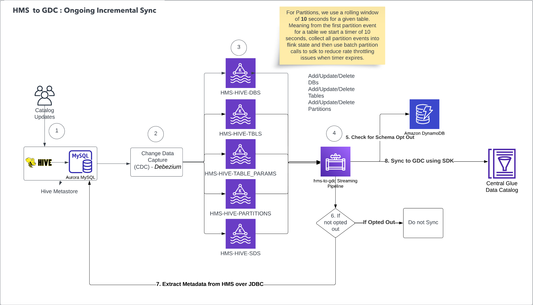
ssh rocky@<<PUBLIC_IP_ADDRESS>> -i <<YOUR_EC2_TEST_KEYPAIR_PEM_FILE>>

When you are logged in to the machine, you can start with password updates and general necessary packages:

# Set a password for your rocky user.
sudo passwd rocky

# Install some useful packages for later use.
sudo yum install wget nano unzip -y

# Install AWS CLI.
# https://docs.aws.amazon.com/cli/latest/userguide/getting-started-install.html
cd ~
curl "https://awscli.amazonaws.com/awscli-exe-linux-x86_64.zip" -o "awscliv2.zip"
unzip awscliv2.zip
sudo ./aws/install

# Install pip.
curl -O https://bootstrap.pypa.io/get-pip.py
python get-pip.py --user

# Make sure all packages are up-to-date.
sudo yum update -y

# Install GNOME.
sudo yum groupinstall "Server with GUI" -y

# Install kernel-devel and reboot.
sudo yum install kernel-devel -y
sudo reboot

Reconnect to the instance to disable nouveau drivers, in preparation for installing the GPU drivers:

# We need to disable the nouveau driver which conflicts with NVIDIA graphics cards.
# Make a module configuration to disable it.
sudo nano /etc/modprobe.d/nvidia_nouveau_off.conf

# Add the following lines
blacklist nouveau
options nouveau modeset=0

# CTRL-X and "y" to exit and save changes

# Ensure this file is also in usr/lib.
sudo cp /etc/modprobe.d/nvidia_nouveau_off.conf /usr/lib/modprobe.d/

# Rebuild the initramfs / boot process.
sudo dracut --force

# Set a new boot config based on the running system, and reboot.
sudo grub2-mkconfig -o /boot/grub2/grub.cfg
sudo reboot

Reconnect to the instance to begin installing the GPU drivers:

# Firstly, you can now double check that nouveau is not present on the system.
# You should see no output from the below:
lsmod | grep nouveau

You must use AWS approved NVIDIA GPU drivers, issued through Amazon S3, not only for optimal compatibility and performance, but also to make sure that the necessary professional GRID drivers are automatically provisioned:

https://docs.aws.amazon.com/AWSEC2/latest/UserGuide/install-nvidia-driver.html

At the time of writing, these are the current steps to install the correct NVIDIA GPU drivers.

# Install supporting libraries for NVIDIA GRID driver.
sudo dnf install -y make gcc elfutils-libelf-devel libglvnd-devel kernel-devel-$(uname -r)

mkdir ~/nvidia
cd ~/nvidia

# Copy the latest GRID driver from the public AWS S3 bucket.
aws s3 cp --recursive s3://ec2-linux-nvidia-drivers/latest/ .
chmod +x NVIDIA-Linux-x86_64*.run
sudo /bin/sh ./NVIDIA-Linux-x86_64*.run

# Follow the prompts to install:
# - you do not need to install 32 bit drivers
# - you should rebuild initramfs if requested.

# Check the driver is installed.
nvidia-smi -q | head

You should get an output as follows:

==============NVSMI LOG==============

Timestamp : Wed Jan 8 13:56:10 2025
Driver Version : 550.127.05
CUDA Version : 12.4
Attached GPUs : 1
GPU 00000000:31:00.0
Product Name : NVIDIA L4

Now set up the Amazon DCV server to stream the desktop to your local machine/client.

# Installing Amazon DCV.
# You can follow more detailed / up-to-date instructions at this link:
# https://docs.aws.amazon.com/dcv/latest/adminguide/setting-up-installing-linux-server.html

# First, disable the Wayland protocol.
sudo nano /etc/gdm/custom.conf
# Uncomment the "WaylandEnable=false" line.
# CTRL-X and "y" to exit and save changes

# Configure X Server -- check that the system is configured for graphical sessions:
sudo systemctl get-default
# If "multi.target" is returned then perform the following:
sudo systemctl set-default graphical.target

# start the X server
sudo systemctl isolate graphical.target

# Update xorg.conf with multi monitor connectivity.
sudo nvidia-xconfig --preserve-busid --enable-all-gpus --connected-monitor=DFP-0,DFP-1,DFP-2,DFP-3

# Restart X-Server.
sudo systemctl isolate multi-user.target
sudo systemctl isolate graphical.target

# Download and install the Amazon DCV server
mkdir ~/amazondcv
cd ~/amazondcv

# Install the key
sudo rpm --import https://d1uj6qtbmh3dt5.cloudfront.net/NICE-GPG-KEY

# Get the latest Rocky 9 Amazon DCV server.
# Note: The Amazon DCV team provide permanent links to the latest DCV software:
# https://www.amazondcv.com/latest.html
wget https://d1uj6qtbmh3dt5.cloudfront.net/nice-dcv-el9-x86_64.tgz
tar -xvzf ./nice-dcv-el9-x86_64.tgz

# 'cd' into the extracted folder -- note this will be version named, hence the generic line below.
cd $(ls -d */|head -n 1)

# install the server rpm -- note this will be version named, hence the generic line below.
sudo yum install $(ls nice-dcv-server*.rpm|head -n 1)

# Restart the X Server.
sudo systemctl isolate multi-user.target
sudo systemctl isolate graphical.target

The Amazon DCV server uses parameters to specify configuration options. On Linux this manifests as a file on disk.

# Adjust the Amazon DCV config files to enable
# the automatic creation of a session by the "rocky" user...
sudo nano /etc/dcv/dcv.conf

# Under [session-management] add the following line:
create-session = true

# Under [session-management/automatic-console-session] add the following line:
owner = "rocky"

# CTRL-X and "y" to exit and save changes.

# Start DCV and enable it to automatically restart on boot
sudo systemctl restart dcvserver
sudo systemctl enable dcvserver

# Finally, open up the firewall to allow Amazon DCV access.
sudo firewall-cmd --add-port=8443/tcp --permanent
sudo firewall-cmd --add-port=8443/udp --permanent
sudo firewall-cmd --reload

Note: Looking to the future of Linux based workstations, DCV now supports Wayland display drivers on RHEL 10, Rocky Linux 10, CentOS 10 and Ubuntu 26.04.

Now install the Wacom drivers:

mkdir ~/wacom
cd ~/wacom

# Download the drivers from (again replacing the link below with the latest version):
# https://github.com/linuxwacom/input-wacom/releases
wget https://github.com/linuxwacom/input-wacom/releases/download/v1.3.0/input-wacom-1.3.0.tar.bz2
tar jxf input-wacom-1.3.0.tar.bz2
cd input-wacom-1.3.0
sudo su
./configure
make && make install
modprobe wacom
dracut --force

# Setup Wacom Pressure Sensitivity
nano /etc/X11/xorg.conf.d/99-wacom-pressure2k.conf

# Add the following lines:
Section "InputClass"
    Identifier "Wacom pressure compatibility"
    MatchDriver "wacom"
    Option "Pressure2K" "true"
EndSection

# CTRL-X and "y" to exit and save changes.

# Setup Wacom with Amazon DCV and Pressure Sensitivity
# Described here: https://docs.aws.amazon.com/dcv/latest/adminguide/enable-stylus.html
sudo nano /etc/X11/xorg.conf

# Add these 2 sections to the end of the file
Section "InputDevice"
    Identifier "DCV Stylus Pen"
    Driver "dcvinput"
    Option "Pressure2K" "true"
EndSection

Section "InputDevice"
    Identifier "DCV Stylus Eraser"
    Driver "dcvinput"
    Option "Pressure2K" "true"
EndSection

# Add the following inside the ServerLayout section
InputDevice "DCV Stylus Pen"
InputDevice "DCV Stylus Eraser"

# CTRL-X and "y" to exit and save changes.

# Restart X display
sudo systemctl isolate multi-user.target
sudo systemctl isolate graphical.target

The local instance store NVMe devices need mounting. For more information, visit the Amazon EC2 User Guide.

# View the volumes -- note that only our nvme0n1 drive is available.
# Our secondary instance store is not listed.
df -h

Filesystem      Size  Used Avail Use% Mounted on
devtmpfs        4.0M     0  4.0M   0% /dev
tmpfs           7.4G     0  7.4G   0% /dev/shm
tmpfs           3.0G  1.3M  3.0G   1% /run
efivarfs        128K  3.8K  120K   4% /sys/firmware/efi/efivars
/dev/nvme0n1p4   49G   45G  3.9G  93% /
/dev/nvme0n1p3  936M  716M  221M  77% /boot
/dev/nvme0n1p2  100M  7.0M   93M   8% /boot/efi
tmpfs           1.5G   52K  1.5G   1% /run/user/42
tmpfs           1.5G   36K  1.5G   1% /run/user/1000

# View volumes mapped but not formatted or mounted.
# Note nvme1n1 -- our instance store - is listed but not mounted.
lsblk

NAME        MAJ:MIN RM   SIZE RO TYPE MOUNTPOINTS
nvme0n1     259:0    0    50G  0 disk 
├─nvme0n1p1 259:2    0     2M  0 part 
├─nvme0n1p2 259:3    0   100M  0 part /boot/efi
├─nvme0n1p3 259:4    0  1000M  0 part /boot
└─nvme0n1p4 259:5    0  48.9G  0 part /
nvme1n1     259:1    0 558.8G  0 disk

# Create a file system on that device
sudo mkfs -t xfs /dev/nvme1n1

# Create a directory to mount the new device.
sudo mkdir /data

# Mount the device to your new directory.
sudo mount /dev/nvme1n1 /data

# Confirm our instance store - nvme1n1 - is now mounted.
df -h

Filesystem      Size  Used Avail Use% Mounted on
devtmpfs        4.0M     0  4.0M   0% /dev
tmpfs            31G     0   31G   0% /dev/shm
tmpfs            13G  1.2M   13G   1% /run
efivarfs        128K  3.8K  120K   4% /sys/firmware/efi/efivars
/dev/nvme0n1p4   49G   44G  5.1G  90% /
/dev/nvme0n1p3  936M  716M  221M  77% /boot
/dev/nvme0n1p2  100M  7.0M   93M   8% /boot/efi
tmpfs           6.1G   36K  6.1G   1% /run/user/1000
/dev/nvme1n1    559G  4.0G  555G   1% /data

Finally, we show some examples of application-specific library setup. Each application potentially has its own list of necessary libraries to install, which can be referenced online. The following are some examples:

# SideFX Houdini :
# https://www.sidefx.com/Support/system-requirements/linux-package-requirements-for-houdini-205/
sudo yum install alsa-lib compat-openssl11 dbus-libs expat fontconfig glibc libatomic libevent libglvnd-glx libglvnd-opengl libICE libSM libX11 libX11-xcb libxcb libXcomposite libXcursor libXdamage libXext libXfixes libXi libxkbcommon libxkbcommon-x11 libXrandr libXrender libXScrnSaver libXt libXtst libzstd nspr nss nss-util openldap pciutils-libs tbb xcb-util xcb-util-image xcb-util-keysyms xcb-util-renderutil xcb-util-wm zlib -y

# Autodesk Maya
# https://help.autodesk.com/view/MAYAUL/2025/ENU/?guid=GUID-D2B5433C-E0D2-421B-9BD8-24FED217FD7F
sudo yum install epel-release -y
sudo yum install libnsl.x86_64 audiofile-dev compat-openssl11 gtk2 libffi libmng libglvnd-opengl libpng15 libpq libXp mesa-libGLU xcb-util-cursor xcb-util-wm xcb-util-image xcb-util-keysyms xcb-util-renderutil xorg-x11-fonts-ISO8859-1-75dpi xorg-x11-fonts-ISO8859-1-100dpi -y

And lastly, it is time to clean up.

cd ~
rm -rf ~/nvidia
rm -rf ~/amazondcv
rm -rf ~/Wacom

# Reboot before logging in
sudo reboot

Logging in to your workstation

To log in to your machine using Amazon DCV, you must set up the client software on your local machine:

  1. On your local machine/laptop, open the Amazon DCV download webpage.
  2. Expand the Amazon DCV Client entry that matches the Server version that you installed on your workstation.
  3. Choose the relevant OS for your machine/laptop, for example Windows (x86_64).
  4. Download the installer.
  5. Run the installer.

When it is installed, we need to determine the Public IP address of the workstation to connect to:

  1. In the Amazon EC2 Console, choose Amazon EC2 Dashboard.
  2. Choose Instances (running).
  3. Choose the “my_linux_workstation” EC2 instance, in the top pane of the screen.
  4. Choose the copy icon next to the Public IPv4 address in the lower pane to copy the IP address.

Finally, use the Amazon DCV client to view the workstation:

  1. Open the Amazon DCV client on your local machine.
  2. Paste the preceding IP address and press Enter, then trust the connection.

  3. You will see a security warning about an untrusted certificate. This is expected behavior because DCV uses a self-signed certificate by default. For this initial setup, it’s safe to accept the certificate and proceed with the connection. For a detailed explanation of why this warning appears and how to implement proper certificate security for production environments, see Amazon DCV Connection Security in Building a GPU workstation for visual effects with Amazon EC2: Part 5 – Security.
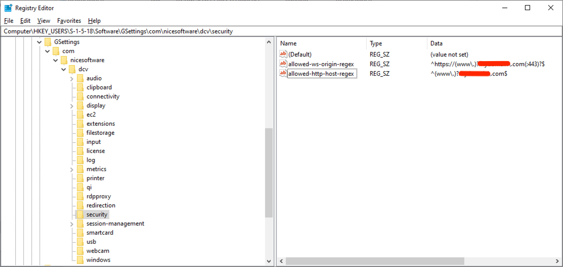
  4. In the next Username / Password entry field, choose rocky, and the appropriate password to which you set that user.

After the connection is established, Amazon DCV opens and displays the remote workstation desktop. The following screen capture shows the running workstation, confirming that your remote session is active and the environment is ready to use. In this example, the Rocky Linux desktop is shown with SideFX Houdini open, displaying a rendered scene in the viewport against the Rocky Linux desktop background.

Rocky Linux workstation desktop running SideFX Houdini with a rendered scene in the viewport

Figure 2: A screen capture of a Rocky Linux-based workstation

Cleaning up

Finally, you must turn off your instances when not in use, either through the AWS Management Console, or through other programmatic methods such as the AWS Command Line Interface (AWS CLI). You incur costs associated with a running machine, and so deactivating machines when not in use reduces your expenditure.

Deactivating instances can be done by choosing Terminate instance from the Instance state options of the workstation on the Amazon EC2 console. The instance shuts down and reports a “Terminated” state on the console, but it automatically disappears after a short time.

However, if you want to learn more about the various methods to deactivate an EC2 instance, and creating a persistent machine image of your Linux instance, then refer to Part 4 of the series: Building a GPU workstation for visual effects with Amazon EC2: Part 4 – Optimizations. Additionally, Part 4 will cover essential information on security practices for Linux EC2 instances, including build-time hardening and automated patch management to protect your workstation infrastructure from evolving threats.

Conclusion

In this post you have subscribed to and deployed an AWS Marketplace AMI of Rocky Linux to serve as your base image. Then, you modified it with GPU drivers, Wacom drivers, and other modules to make it a capable Linux-backed VFX workstation, using Amazon EC2 GPU accelerated G instance types.

You may also be interested in Part 3 of our series, Building a GPU workstation for visual effects with Amazon EC2: Part 3 – Windows, to learn how to create a Windows-backed VFX workstation.
We also recommend that you continue to Part 4 of our series, Building a GPU workstation for visual effects with Amazon EC2: Part 4 – Optimizations, to learn how to implement GPU optimizations and infrastructure to streamline the provisioning of workstations.

For more information contact us at .

Further reading

If you want to augment a VFX workstation environment with a dedicated render farm, then consider the managed service AWS Deadline Cloud.

EC2 instance metrics, such as CPU and memory usage, are readily sent to Amazon CloudWatch logs, so you can access this data through the console and AWS CLI. This information can be pertinent to discern if an EC2 instance is being over-provisioned or under-provisioned for the work at hand. An over-provisioned instance has excessive CPU, memory, and networking resources for the current tasks and could be optimized for price. Alternatively, an under-provisioned instance does not have enough resources to cope. For more information visit the Amazon EC2 User Guide.

More advanced examples of using Amazon DCV can be found in the aws-samples GitHub repo. This includes methods to broker multiple users and instances. Furthermore, DCV Connection Gateway provides a single entry point so you can connect to multiple DCV sessions across different instances, streamlining access management and improving security through centralized authentication.
Commercial options also exist to perform artist/instance brokering, using Amazon DCV and Amazon EC2 Launch templates. An example of such an offering is Leostream.

For reference, examples of setting up Amazon DCV capable instances, using AWS CloudFormation templates as a method of deployment, can be found in this GitHub repo.

A greater depth of analysis of bit rates and latency surrounding Amazon DCV connections can be found in this AWS HPC post.


About the authors

Andy Hayes

Andy Hayes

Andy is a Senior Visual Computing Solutions Architect at AWS. With 20 years’ experience in Visual Effects and Animation, Andy has led CG divisions and departments and added supervision to film projects, earning both Annie and Visual Effects Society Awards along the way. At AWS, he partners with studios and creative technology companies across the Media & Entertainment industry, spanning VFX and animation to rendering, virtual production, and games, helping them design and scale the cloud infrastructure and workflows behind their content pipelines. Drawing on his production background, Andy bridges the worlds of artists and engineers, guiding customers as they adopt technologies like high-performance rendering, GPU compute, and increasingly AI and machine learning to solve real creative and technical challenges. He remains passionate about the marriage of art and science that leads to the creation of compelling imagery, and about aligning technology to the evolving needs of the industry.

Mike Owen

Mike Owen

Mike is a Principal Visual Computing Solutions Architect at AWS, where he has spent many years helping studios move their creative work to the cloud. He focuses on the architecture behind high-end content creation: cloud workstations, render farm scaling and storage that spans multiple sites. Mike works with studios and creative technology companies across Media & Entertainment, from VFX and animation to finishing and colour. He has pioneered the concept of “Studio in the Cloud” and helped bring industry tools such as Autodesk Flame to AWS, and has contributed to a range of AWS Thinkbox Deadline improvements. Most recently he has led development of KNFSD File Cache, an open-source NFS caching solution from AWS. It lets studios burst large render workloads into the cloud whilst their data stays on existing on-premises storage. He cares about giving artists the same seamless, colour-accurate experience in the cloud that they expect on-premises, and about removing the cost and complexity that usually come with building a global studio.

Build a GPU workstation for visual effects on Amazon EC2: Part 1 – Setup

Post Syndicated from Andy Hayes original https://aws.amazon.com/blogs/compute/build-a-gpu-workstation-for-visual-effects-on-amazon-ec2-part-1-setup/

For many years Amazon Web Services (AWS) has been guiding users in the deployment of powerful NVIDIA GPU-backed workstations for graphics-intensive workloads. With the recent expansion of our G-series Amazon Elastic Compute Cloud (Amazon EC2) graphics-based instances, we’re excited to introduce new instance families that deliver enhanced performance and capabilities. We’re also refreshing our comprehensive guidance on choosing and configuring these powerful virtual workstations.

This is the first in a five-part series providing detailed guidance on instance types, and deployment instructions for building Windows and Linux based NVIDIA GPU powered workstation on GPU accelerated EC2 instances. In this initial post, we explore the instance types, and outline essential AWS configurations for account preparation, security, policies, and other prerequisites. Subsequent posts cover Linux deployment (Part 2), Windows deployment (Part 3), optimizations and infrastructure for standardizing workstations deployment at scale (Part 4), and security considerations (Part 5).

G instance families

The Amazon EC2 G-series instances come in multiple families, with various types and fractionalization of GPUs, memory-to-CPU ratios, and sizes of vCPU and RAM. The g6 and gr6 instances, equipped with NVIDIA L4 GPUs, deliver up to 200 percent performance improvement in graphics-intensive workloads compared to the widely-adopted g4dn family, while offering enhanced performance and cost efficiency over their g5 predecessors. The g6f and gr6f options introduce more GPU partitioning capabilities with the NVIDIA L4, so you can provision fractional GPU allocations. This supports more cost-effective scaling for workloads that do not need a full GPU, with options for half, quarter, and one-eighth GPU. Fractional instances are ideal for remote workstation applications for staff that need only partial GPU usage, as well as other tasks such as lightweight machine learning (ML) research.

The g6e instances, featuring the NVIDIA L40S GPU, go further with double the GPU memory, 2.9x faster GPU memory bandwidth, and up to 2.5 times overall performance improvement compared to g5 instances. All three families offer flexible configurations with 1, 4, or 8 GPUs, providing specialized cores optimized for GPU processing, ray tracing, and machine learning workloads, as shown in the following figure.

The latest 7th generation instances, the g7 and g7e offer greater performance in GPU speed and memory with the latest NVIDIA RTX PRO 4500 and 6000 respectively. These instances are well suited for high-end 3D and 2D workloads and artificial intelligence (AI) workloads, delivering 4.6 times the AI inference performance of previous g6 instances. With up to 700 Gbps EFA-enabled network bandwidth, g7 instances help you run graphics and data workloads more efficiently.

NVIDIA
L4
NVIDIA
L40S
NVIDIA
RTX PRO 4500
NVIDIA
RTX PRO 6000
Architecture Ada Lovelace Ada Lovelace Blackwell Blackwell
Memory 24 GB GDDR6 48 GB GDDR6 32 GB GDDR7 96 GB GDDR7
Memory Bandwith 300 GB/s 864 GB/s 896 GB/s 1790 GB/s
Cuda Cores 7680 18176 10496 24064
Tensor Cores 240 568 328 752
Ray Tracing Cores 60 140 82 188

Figure 1: The list of GPU architecture statistics for the L4, L40S, RTX PRO 4500, and RTX PRO 6000 NVIDIA GPUs

The 6th and 7th generation of G instances are available in multiple configurations to accommodate diverse GPU, CPU, memory, and networking requirements. The g6, g6f, and g7 instances maintain the traditional 1:4 ratio of vCPUs to memory (GiB) established by previous generations such as g4dn and g5. The gr6 and gr6f families introduce an enhanced 1:8 ratio option, while the g6e and g7e instances natively possess the expanded 1:8 ratio. These higher allocations suit memory-intensive 2D and 3D workloads that frequently encounter memory constraints, providing support for demanding visual computing applications.

For the non-fractional g6 and gr6 instances, the configurations of sizes are as follows:

Instance type NVIDIA L4 GPU count vCPUs Memory (GiB) EBS Bandwidth (Gbps) Network Bandwidth (Gbps)
Single GPU g6.xlarge 1 4 16 Up to 5 Up to 10
g6.2xlarge 1 8 32 Up to 5 Up to 10
g6.4xlarge 1 16 64 8 Up to 25
g6.8xlarge 1 32 128 16 25
g6.16xlarge 1 64 256 20 25
Single GPU / Memory Biased gr6.4xlarge 1 16 128 8 Up to 25
gr6.8xlarge 1 32 256 16 25
Multi GPU g6.12xlarge 4 48 192 20 40
g6.24xlarge 4 96 384 30 50
g6.48xlarge 8 192 768 60 100

Figure 2: The list of g6 and gr6 instance types with corresponding GPU amounts, vCPUs, network, and bandwidth data

The fractional g6f and gr6f configurations are:

Memory (GiB) to vCPU ratio Instance type NVIDIA L4 GPU count NVIDIA L4 GPU RAM (GiB) vCPUs Memory (GiB) EBS Bandwidth (Gbps) Network Bandwidth (Gbps)
4-to-1 g6f.large 1/8 3 2 8 Up to 5 Up to 10
g6f.xlarge 1/8 3 4 16 Up to 5 Up to 10
g6f.2xlarge 1/4 6 8 32 Up to 5 Up to 10
g6f.4xlarge 1/2 12 16 64 6 Up to 25
8-to-1 gr6f.4xlarge 1/2 12 16 128 8 Up to 25

Figure 3: The list of g6f and gr6f instance types with corresponding fractional GPU amounts, vCPUs, network, and bandwidth data

For the g7 instances, the configurations of sizes are as follows:

Instance type NVIDIA RTX PRO 4500 GPU count vCPUs Memory (GiB) EBS Bandwidth (Gbps) Network Bandwidth (Gbps)
Single GPU g7.2xlarge 1 8 32 Up to 8 Up to 60
g7.4xlarge 1 16 64 8 Up to 100
g7.8xlarge 1 32 128 16 100
Multi GPU g7.12xlarge 2 48 192 20 175
g7.24xlarge 4 96 384 40 350
g7.48xlarge 8 192 768 80 700
g7.metal* 8 192 768 80 700

* Coming soon

Figure 4: The list of g7 instance types with corresponding GPU amounts, vCPUs, network, and bandwidth data

For the enhanced g6e the following instance size configurations are:

Instance type NVIDIA L40S GPU count vCPUs Memory (GiB) EBS Bandwidth (Gbps) Network Bandwidth (Gbps)
Single GPU g6e.xlarge 1 4 32 Up to 5 Up to 20
g6e.2xlarge 1 8 64 Up to 5 Up to 20
g6e.4xlarge 1 16 128 8 20
g6e.8xlarge 1 32 256 16 25
g6e.16xlarge 1 64 512 20 35
Multi GPU g6e.12xlarge 4 48 384 20 100
g6e.24xlarge 4 96 768 30 200
g6e.48xlarge 8 192 1536 60 400

Figure 5: The list of g6e instance types with corresponding GPU amounts, vCPUs, network, and bandwidth data

Moreover, the g7e has the following instance size configurations:

Instance type NVIDIA L40S GPU count vCPUs Memory (GiB) EBS Bandwidth (Gbps) Network Bandwidth (Gbps)
Single GPU g7e.2xlarge 1 8 64 Up to 5 50
g7e.4xlarge 1 16 128 8 50
g7e.8xlarge 1 32 256 16 100
Multi GPU g7e.12xlarge 2 48 512 25 400
g7e.24xlarge 4 96 1024 50 800
g7e.48xlarge 8 192 2048 100 1600

Figure 6: The list of g7e instance types with corresponding GPU amounts, vCPUs, network, and bandwidth data

EC2 instances mount one (or more) Amazon Elastic Block Store (Amazon EBS) volumes for durable, block-level storage. These can be detached from the instance and retained independently from the lifecycle of that instance, allowing modifications of the instance itself (such as changing the size and type) without the loss of storage.

Ephemeral NVMe storage on each instance is also provided by Instance Stores, aligned for temporary scratch data that benefits from performant local I/O access, which can be used by 2D/3D applications (for example Foundry Nuke’s cache directory). In the follow-up posts we discuss setting up and configuring these instance stores to maximize efficiency. The 6th and 7th generation EC2 instances automatically have instance stores allocated, dependent on their sizes, as shown in the following figure:

Instance Type Instance store volumes
g6f.large, g6f.xlarge 1 x 100GB
g6f.2xlarge 1 x 200 GB
g6.xlarge, g6e.xlarge 1 x 250 GB
g6.2xlarge, g6e.2xlarge, g6f.4xlarge, gr6f.4xlarge 1 x 450 GB
g6.4xlarge, g6e.4xlarge, gr6.4xlarge, g7.2xlarge, g7.4xlarge 1 x 600 GB
g6.8xlarge, g6e.8xlarge, gr6.8xlarge 2 x 450 GB
g6.12xlarge, g6e.12xlarge 4 x 940 GB
g6.16xlarge, g6e.16xlarge 2 x 940 GB
g6.24xlarge, g6e.24xlarge 4 x 940 GB
g6.48xlarge, g6e.48xlarge 8 x 940 GB
g7.8xlarge 1 x 950 GB
g7.12xlarge, g7e.2xlarge, g7e.4xlarge, g7e.8xlarge 1 x 1.9 TB
g7.24xlarge, g7e.12xlarge 1 x 3.8 TB
g7.48xlarge, g7.metal*, g7e.24xlarge 2 x 3.8 TB
g7e.48xlarge 4 x 3.8 TB

* Coming soon

Figure 7: The configuration of instance stores on the 6th and 7th generation EC2 instances

The 6th and 7th generation G instances represent our latest offering in GPU-powered workstations capable servers, but we still offer previous generations, notably the g5 and g4dn, giving many choices in machine types to match performance and cost needs.

You can find specifications of all our instances types, on our Amazon EC2 webpage (G instances are classed as Accelerated Computing types).

Desktop streaming with Amazon DCV

Typically, cost-effective Mini PCs or laptops are used to connect to the Amazon EC2 workstation through a desktop streaming protocol. AWS offers a high-end desktop experience through Amazon DCV. This is a performant remote display protocol capable of streaming 4k UHD resolution images over multiple monitors (up to 4), 60 frames per second, QUIC UDP support for high performance image streaming, 4:4:4 8-bit chroma sub-sampling, and stylus/touch device support for M&E workloads. Our posts show how to set up both the server and client for Amazon DCV on Windows and Linux.

The recent addition of Wacom Bridge with Amazon DCV has optimized stylus operations further (on Windows at the time of writing, Linux in beta currently). This is both in terms of real-time user feedback on the local device, mitigating the effect of any potential latency delay, but also dedicated channel support for hardware communications to provide even lower latency performance, as well as the synchronization of settings.

Workstation connectivity

When establishing connectivity between your on-premises workstation and your EC2 instance, you have three primary options, each offering different levels of security, performance, and complexity.

Internet connectivity (used in this post)

For this post, we use the most basic connection method: direct internet connectivity. This approach connects your local workstation to your Amazon EC2 instance over the public internet, with security groups (virtual firewalls) configured to restrict access to your specific IP address and only the necessary ports.

This method uses application-layer security to provide built-in encryption for all Amazon DCV streaming sessions, which helps keep your visual data protected during transmission. Security groups operate at the network and transport layers to control which IP addresses and ports can reach your instances. Together, these layers provide complementary security properties:
  • Confidentiality in transit: DCV session traffic is encrypted, which helps prevent an intermediary who intercepts the traffic from reading its contents.
  • Access control at the instance boundary: Security groups accept connections only from IP addresses on your approved list, reducing the instance’s exposure to unsolicited inbound connection attempts.
  • Reduced attack surface: Only the specific ports required for DCV are exposed, which limits how much of the instance is reachable from the network.

This method provides a straightforward setup suitable for individual users or small teams, combining quick configuration with secure encrypted streaming. We discuss the security group configuration in detail later in this post.

The following diagram illustrates this internet-based connectivity architecture. It shows how an artist’s local workstation connects across the public internet to a GPU-backed EC2 instance in AWS, with Amazon DCV carrying the session between them.

Architecture diagram of on-premises Windows and Linux workstations connecting over the public internet through Amazon DCV to GPU-backed Amazon EC2 instances in an Amazon VPC

Figure 8: A streamlined architectural diagram showing on-premises and home workstations integrating with Amazon EC2 instances, using Amazon Machine Images and EBS storage, connecting through the internet

VPN connectivity

For organizations requiring additional security beyond basic internet connectivity, AWS Site-to-Site VPN provides encrypted tunnels that use the internet securely. This method creates a secure connection between your on-premises location and your AWS resources, allowing you to access EC2 workstations through encrypted channels while maintaining the high-performance capabilities needed for graphics-intensive work.

AWS Site-to-Site VPN adds network-layer encryption on top of the application-layer protection provided by Amazon DCV. The VPN establishes encrypted IPsec tunnels between your on-premises network and AWS, so traffic is protected at the network layer before it reaches the application. In practice this means your DCV session traffic travels inside an additional encrypted tunnel alongside the rest of your network connection.
Choosing Site-to-Site VPN over direct internet connectivity comes down to a few practical factors:

  • Security posture: VPN extends your existing corporate network controls and policies into AWS, so the same governance you apply on-premises continues to apply to traffic reaching your instances. This is useful if your organization requires network-layer encryption or treats AWS as an extension of the internal network.
  • Operational complexity: VPN requires configuring and maintaining the tunnel, a customer gateway, and routing on both sides. This is more involved than direct connectivity, which needs only a security group.
  • Cost: Site-to-Site VPN carries an hourly connection charge plus data transfer.

VPN connectivity is a good fit when you need to extend your corporate network into AWS and maintain consistent security policies across both environments, and when the added setup and cost are justified by that requirement.

The following diagram shows the VPN-based connectivity architecture. The key difference from the direct-internet setup is that the EC2 instances now sit in a private subnet with no public internet access. The Site-to-Site VPN carries all traffic between your on-premises network and AWS instead.

Architecture diagram of on-premises workstations connecting through an IPsec Site-to-Site VPN to GPU-backed Amazon EC2 instances in a private subnet

Figure 9: A streamlined architectural diagram showing on-premises and home workstations integrating with Amazon EC2 instances, using Amazon Machine Images and EBS storage, connecting through a Site-to-Site VPN

AWS Direct Connect

For workloads that need consistent network performance and a connection that doesn’t traverse the public internet, AWS Direct Connect establishes a dedicated physical connection between your on-premises location and AWS. Through your chosen network provider, it creates a private link from your premises to the AWS Region containing your Amazon EC2 G instances, which can offer more predictable latency and bandwidth than an internet-based connection.

AWS Direct Connect provides additional isolation at the physical and data link layers by using a dedicated connection that doesn’t traverse the public internet. Your traffic travels over private network infrastructure between your location and AWS, which keeps it off shared internet paths and gives you more consistent, predictable network behavior than an internet-based connection. Because the connection is private and dedicated, it isn’t exposed to the general internet in the way a public connection is.

AWS Direct Connect is ideal for organizations requiring consistent network performance, enhanced security, and reduced data transfer costs when working with graphics workstations in the cloud. Combined with the application-layer encryption of Amazon DCV, this provides defense-in-depth across the entire network stack, from the physical cables through to the application data itself. This approach provides the most predictable latency and bandwidth for demanding creative workflows.

The following diagram depicts the Direct Connect connectivity architecture. As with the VPN option, the EC2 instances sit in private subnets with no need for public internet access, but here the connection runs over a dedicated Direct Connect link between your on-premises location and AWS.

Architecture diagram of on-premises workstations connecting over an AWS Direct Connect link to GPU-backed Amazon EC2 instances in a private subnet

Figure 10: A streamlined architectural diagram showing on-premises and home workstations integrating with Amazon EC2 instances, using Amazon Machine Images and EBS storage, connecting through a Direct Connect link

Consult the documentation for further details and options around VPN offerings, as well as Direct Connect, to inform your security decisions. For further information, and additional firewall and protection services that can enhance protection against exploits such as ransomware and DDoS, please see Security, Identity and Compliance on AWS.

Latency

A superior virtual workstation experience relies on low-latency and high-bandwidth connectivity from your local client to your EC2 instance. Bandwidth requirements vary based on several factors such as the number of monitors, screen resolution, frame rate, and visual quality settings. For creative professionals using Wacom tablets or similar input devices, we recommend a latency round trip of 50 ms or less when using Amazon DCV. To evaluate your connection’s suitability, there are a number of third-party websites that you can use to test latency between your location and the nearest Region, such as https://aws-latency-test.com/ or https://www.cloudping.info/.

“Our collaboration with the AWS Visual Computing team and the use of EC2 instances as virtual workstations, has exceeded our expectations, delivering exceptional result.”

— John Coyne, Senior Technical Manager, Sky TV

Workstation build overview

For the purposes of this post, we focus on deploying a g6 family instance.

The following overview outlines the complete build across the whole series. Part 1 covers the prerequisites and base image selection. The remaining phases such as the instance configuration, creating Amazon Machine Images, and setting up launch templates are covered in later parts.

  1. Prerequisites.
    • Account setup and GPU instance quotas.
    • Security configurations (access, firewalls, permissions).
  2. Base image selection.
    • Linux and Windows options.
    • Customization for VFX needs.
  3. Instance configuration.
    • Linux and Windows set up.
    • GPU and system tools installation.
  4. Creating Amazon Machine Images (AMIs) to capture the resultant machine image.
  5. Setting up EC2 Launch Templates to encapsulate all boot requirements.
    • Standardizing deployment parameters.
    • Streamlining future workstation launches.
  6. GPU optimization tips and resources.

Cost consideration

In these posts we use different AWS services, with each service having a cost associated with its usage. EC2 instances are charged by the second, so you must make sure that you shut down or terminate the instances when you are finished to avoid unwanted costs.

Accessing AWS services through the AWS Command Line Interface

AWS has many API/SDK entry points for creating and manipulating services. In this post we use the AWS Command Line Interface (AWS CLI), a convenient utility that you can use to query and set AWS service properties through the command line. In both the Windows and Linux deployment posts we set up the CLI for later convenience.

For more information about how to configure the credentials for usage with the CLI, as well as the range of functionality that you can use with it, go to the AWS CLI User Guide.

Workstation prerequisites Part 1: account setup and service quotas

The following steps are used to set up a secure Amazon Virtual Private Cloud (Amazon VPC) network platform for your instances, providing security and permissions for accessing and configuring your instance:

  1. Create an AWS account.
  2. Open and configure the AWS Management Console to gain access to AWS.
    • Go to the Console.

Setting the AWS Region

At the time of writing, AWS has 39 geographic Regions, each composed of multiple AWS Availability Zones (AZs) to make sure of service availability and durability, and over 35 AWS Local Zones (which are infrastructure deployments that place compute, storage, and other select AWS services closer to large population and industry centers). For more information, see the AWS Documentation on Global Infrastructure. As we previously mentioned, latency can be critical for optimal virtual workstation experiences. Therefore, we recommend building your workstations in a Region that offers the best latency experience. This is configured on the console itself:

  1. Choose your AWS Region that best suits your needs (a drop down of AWS Regions is available at the top right of the Console).

AWS services can vary across AWS Regions, so before proceeding you must confirm that g6 instances are available in your AWS Region of choice. This can be done through the Amazon EC2 service page, as shown in the following figure:

  1. Open the Amazon EC2 service page, the central service page for deploying EC2 instances.
    • Search for “EC2” in the Service search bar (top left), or choose Services -> Compute -> EC2.
  2. Choose Instance Types in the left pane.
  3. Enter “g6” into the Instance Types search bar and confirm that the various g6 instance types are listed as available in that AWS Region. The following image shows a filtered response from the Instance Types pane.
Amazon EC2 Instance Types console page filtered to show the available g6 instance types in a Region

Figure 11: A screen capture of the Instance Types page, reporting g6 Amazon EC2 availability in a Region

Service limits

Limits exist around many AWS services. They act as guard rails for new users and prevent misuse of AWS services. New AWS accounts start with low limits to prevent unintentional spend, so you need to check the account limits to make sure that there is enough GPU vCPU quota to launch your workstation. You can check and request limit changes through the Service Quotas service page:

  1. Navigate to the Service Quotas page by searching for its name in the Services search bar (top left of the Console window). Or alternatively choose Services -> Management and Governance -> Service Quotas.

You can choose the star icon next to each service to bookmark it for access later at the top of the Console.

  1. Under Manage quotas (top right), enter EC2 in the search field, choose Amazon Elastic Compute Cloud (Amazon EC2), and choose View quotas.
  2. In the Service quotas search field that appears, enter On-Demand G and the list of quotas should reduce to just Running On-Demand G and VT instances, the quota controlling your access to G instance machines, as shown in the following figure.
Service Quotas console showing the Running On-Demand G and VT instances quota with an applied value of 64

Figure 12: A screen capture of the Service Quotas page, requesting an increase to the GPU limit

You can see the current Applied account-level quota value, which is your limit on how many vCPUs you can use at any given time in this Region. This is not the number of instances (a common misconception)! We recommend making sure that you have at least a quota of 32, because this is enough to run two g6.4xlarge instances, a common size that suits basic 2D and 3D workflows. If the value in the applied account-level quota is below this, then you must submit a request to increase it:

  1. Choose Request Increase at account level.
  2. Enter “32” in the Increase quota value field.
  3. Choose Request.

When you receive an email confirmation of the increase, check the quota limit again for a value of 32 and you are safe to proceed with the rest of the post.

Workstation prerequisites Part 2: networking and security

When you have received your Service Quota increase, you can continue back in the AWS Management Console to start setting up some auxiliary components needed for workstations, for example security keys, firewall groups, and so on.

  1. Open the Amazon EC2 service page, the central service page for deploying EC2 instances.
    • Search for “EC2” in the Service search bar (top left) or choose Services -> Compute -> EC2.

Amazon EC2 key pair security

Amazon EC2 key pairs are security credentials that validate your identity when accessing EC2 instances.

To set up an Amazon EC2 key pair:

  1. Under Network and Security on the left side of the panel, choose Key Pairs.
  2. Choose Create key pair in the top right.
  3. Give your new key pair a name, for example ec2_test_keypair.
  4. Leave the key pair as an RSA type, with a .pem extension, and choose Create key pair.
  5. Store the automatically downloaded .pem file in a safe place, because you need it later.

You should restrict the permissions on the .pem file so that only you can read it.

On a Mac or Linux machine you can change the permission in a terminal:

chmod 400 <<YOUR_EC2_TEST_KEYPAIR_PEM_FILE>>

On Windows, open the context menu for the file, choose Properties, then the Security tab, choose Advanced, choose Disable inheritance, and remove access to all users except the current user. For more information surrounding the best use of key pairs, go to the relevant section in the Amazon EC2 User Guide.

Virtual firewalls

Security groups act as virtual firewalls, restricting incoming and outgoing traffic to your G instances. You should set up a security group working on the principle of least privilege, which means you must be very specific about which ports and which IP addresses can access it:

  1. Under Network and Security on the left pane, choose Security groups.
  2. Choose Create Security Group in the top left.
  3. Give your security group a name, for example ec2_test_sg.
  4. Give your security group a meaningful description, for example SG for basic EC2 interaction.
  5. Leave the VPC as-is. This automatically presents the ‘default’ VPC in your account and AWS Region.
  6. The following Inbound rules ports must be added to the security group to allow access to that machine from a specific client’s source IP address: in this case your local machine. Under Inbound rules, use the Add rule feature multiple times to add the definitions defined in the following figure, using the My IP drop-down under Source to automatically determine and use your current IP address, appending the /32 CIDR to limit the connectivity to that single address.The following table contains a list of TCP and UDP ports to add to your security group.
Type Protocol Port Range Source Description
SSH TCP 22 <YOUR “CUSTOM” CLIENT SOURCE IP> SSH for Linux platform.
Custom TCP Rule TCP 443 <YOUR “CUSTOM” CLIENT SOURCE IP> HTTPS for both platforms.
Custom TCP Rule TCP 8443 <YOUR “CUSTOM” CLIENT SOURCE IP> Amazon DCV for both platforms.
Custom UDP Rule UDP 8443 <YOUR “CUSTOM” CLIENT SOURCE IP> Amazon DCV for both platforms.
RDP TCP 3389 <YOUR “CUSTOM” CLIENT SOURCE IP> RDP for Windows platform.

Figure 13: The list of inbound ports that need to be opened to allow user access to the EC2 instance for the purpose of this post

For the purposes of this post, we’re making a single security group that encompasses both Linux and Windows. If you’re only focusing on a specific operating system, then a security consideration would be to remove the unneeded ports.
  1. For Outbound rules, the default allows all outbound traffic. This is enough for the instance to download packages and reach AWS service endpoints during setup, and because inbound access is already restricted to your IP, it doesn’t open an inbound path. Open outbound traffic is, however, the route that data exfiltration or a compromised host’s callbacks would use. Once your instance is running and you know which destinations it genuinely needs (for example, HTTPS 443 to AWS and your package repositories), restrict outbound rules to those destinations rather than leaving them fully open.
  2. Choose Create security group to finish making the security group.

Identity and Access Management

AWS advocates a policy of least permissions, establishing a strong base security standpoint, which necessitates that you add the permissions needed for access to services. To allow your Amazon EC2 workstation instance to access services such as Amazon Simple Storage Service (Amazon S3) (for graphics drivers), you must create a role to encompass these permissions for your instance. You should set up an AWS Identity and Access Management (IAM) profile to allow the instance access to the necessary services.

  1. Navigate to the IAM service page by entering “IAM” into the Service search field (top left), or choose Security, Identity & Compliance > IAM.
  2. Choose Roles (in the left side pane).
  3. Choose Create role, in the top right.
  4. Leave the Trusted entity type as AWS service.

You must use AWS approved NVIDIA GPU drivers, issued through Amazon S3, not only for optimal compatibility and performance, but also to make sure that the necessary professional GRID drivers are automatically provisioned. Therefore, you need a role that can read from Amazon S3. You should use a very generic Amazon S3 read-only policy to allow read access to public S3 buckets (such as the bucket on which AWS shares GPU drivers).

  1. Under Use case, enter “S3” and then choose Next (bottom right).
  2. Search for AmazonS3ReadOnlyAccess and choose the box to the left of the policy to add it to the role. Then, choose Next.
  3. Give your new role a name, for example basic_workstation_role.
  4. Choose Create role.
If later on you want to add more service features to your workstation role (for example to enable write permissions from the workstation to one of your own storage buckets), then you can use the same process to add pre-defined permissions or create your own in JSON.

You now have an account, and the resources needed to launch EC2 instances, which are covered in our next posts.

Conclusion

In this post we have discussed the different generation Amazon EC2 instance families: their memory, network, storage, and GPU options. We have outlined the steps needed not only to prepare an AWS account for running GPU workstations but also to build key infrastructure that is needed to deploy them.

We recommend that you continue to Part 2 of our series, Building a GPU workstation for visual effects on Amazon EC2: Part 2 – Linux, where you can learn how to create a Linux-backed workstation. You can also read Part 3 of our series, Building a GPU workstation for visual effects with Amazon EC2: Part 3 – Windows, to learn how to create a Windows-backed workstation.

For more information contact us at .

Further reading

If you want to augment a VFX workstation environment with a dedicated render farm, then consider the managed service AWS Deadline Cloud.

EC2 instance metrics, such as CPU and memory usage, are sent to Amazon CloudWatch, where you can access this data through the AWS Management Console and AWS CLI. This information can be pertinent to discern if an EC2 instance is being over or under provisioned for the work at hand. In other words, it has excessive CPU, memory, and networking resources for the current tasks, and it could be optimized for price, or the alternative where it has not been allocated enough resources to cope. For more information, go to the Amazon EC2 User Guide.

More advanced examples of using Amazon DCV can be found in this “aws-samples” GitHub repo. This includes methods to broker multiple users and instances. Furthermore, DCV Connection Gateway provides a single-entry point for users to connect to multiple DCV sessions across different instances, streamlining access management and improving security through centralized authentication.

Commercial options also exist to perform artist/instance brokering, using Amazon DCV and Amazon EC2 Launch templates. An example of such an offering is Leostream.

For reference, examples of setting up Amazon DCV capable instances, and using AWS CloudFormation templates as a method of deployment, can be found in this GitHub repo.

A greater depth of analysis of bit rates, and latency, surrounding Amazon DCV connections can be found in this AWS HPC post.


About the authors

Andy Hayes

Andy Hayes

Andy is a Senior Visual Computing Solutions Architect at AWS. With 20 years’ experience in Visual Effects and Animation, Andy has led CG divisions and departments and added supervision to film projects, earning both Annie and Visual Effects Society Awards along the way. At AWS, he partners with studios and creative technology companies across the Media & Entertainment industry, spanning VFX and animation to rendering, virtual production, and games, helping them design and scale the cloud infrastructure and workflows behind their content pipelines. Drawing on his production background, Andy bridges the worlds of artists and engineers, guiding customers as they adopt technologies like high-performance rendering, GPU compute, and increasingly AI and machine learning to solve real creative and technical challenges. He remains passionate about the marriage of art and science that leads to the creation of compelling imagery, and about aligning technology to the evolving needs of the industry.

Mike Owen

Mike Owen

Mike is a Principal Visual Computing Solutions Architect at AWS, where he has spent many years helping studios move their creative work to the cloud. He focuses on the architecture behind high-end content creation: cloud workstations, render farm scaling and storage that spans multiple sites. Mike works with studios and creative technology companies across Media & Entertainment, from VFX and animation to finishing and colour. He has pioneered the concept of “Studio in the Cloud” and helped bring industry tools such as Autodesk Flame to AWS, and has contributed to a range of AWS Thinkbox Deadline improvements. Most recently he has led development of KNFSD File Cache, an open-source NFS caching solution from AWS. It lets studios burst large render workloads into the cloud whilst their data stays on existing on-premises storage. He cares about giving artists the same seamless, colour-accurate experience in the cloud that they expect on-premises, and about removing the cost and complexity that usually come with building a global studio.

[$] Additional hardening for the glibc dynamic linker

Post Syndicated from daroc original https://lwn.net/Articles/1105134/

The

Node.js project
recently had a

security vulnerability
that
affected its

Brotli
decoder. The bug

was a buffer overflow
,
but the particular way that official Node.js binaries are built for Linux meant that one of the
main protections against turning a buffer overflow into remote code execution,

address space layout randomization
(ASLR) could not be turned on. If ASLR had been
enabled, the bug would still be exploitable in theory, but much more difficult
to exploit in practice. In response, the GNU C Library (glibc) is

considering
a new set of

tunable settings
to allow administrators to forbid programs that do not
support ASLR. The new settings, while a welcome hardening measure, may not
address the root problem.

Choosing QuePaxa, an unusual consensus algorithm

Post Syndicated from João Pedro Leite original https://blog.cloudflare.com/choosing-quepaxa/

Cloudflare recently announced Meerkat, an experimental distributed consensus service designed to manage our internal global control plane. It is powered by a new consensus algorithm called QuePaxa.

QuePaxa is an unusual choice; most consensus systems use well-established consensus algorithms like Raft, (Multi-)Paxos or Viewstamped Replication. These algorithms are well understood, have mature implementations, and usually work well.

Unfortunately, common consensus algorithms often suffer in wide-area networks with volatile network connectivity and latency, i.e., networks like the Internet, which is where Meerkat runs. These algorithms rely on a single leader process being available and having predictable latency. If the leader goes down, experiences higher latency than usual, or is disconnected, the entire consensus system slows down or becomes unavailable until the leader is replaced. This is unacceptable for Meerkat.

Meerkat’s global deployment environment led us to a newer consensus algorithm, QuePaxa, which promises better stability despite volatility, in large part by not relying on a leader to make progress. In this post we’ll explain why we chose QuePaxa and how the QuePaxa algorithm works.

What we’re building and why it’s unique

Meerkat is a distributed system in which replicas agree upon an ordered log of events, where each event is decided by a consensus algorithm.

Consensus algorithms allow a group of machines to agree on a single shared truth, even if some of those machines crash or disconnect. Consensus algorithms provide an important guarantee: machines never decide conflicting values. This ensures Meerkat replicas’ logs never diverge.

Meerkat uses its consensus-powered log to expose applications like a key-value store, where each entry in the log is a get or a put. Because the consensus algorithm guarantees replicas’ logs never diverge, they all construct the same key-value (KV) state. Comparable consensus-powered systems include Consul, etcd, and Apache ZooKeeper.

Unlike similar systems, however, Meerkat was designed for global scale. A Meerkat cluster may be distributed across continents and connected by links that often exhibit high and variable latency. This is an unusual setup for consensus systems, which are usually deployed in smaller, more local networks, and have strict latency requirements.

The challenges of consensus at a global scale

While all consensus algorithms ensure that replicas agree on the same value, many of them become disproportionately unavailable or slow when network conditions degrade (but machines do not crash). We have seen this happen firsthand: in 2020, the partial failure of a core Cloudflare network switch caused a consensus-powered system to degrade and the dashboard to operate 80x slower than usual, for six hours. Critically, the system lost no data. But it became unavailable for writes until the issue was resolved, which is unacceptable.

Ideally, a consensus algorithm should be able to make progress despite latency spikes and broken connections, not just replica failures. This is particularly a problem at global scale, where faults are more likely to originate in the network, and not our own servers.

Let’s examine two common traits of consensus algorithms that can lead to degradation under hostile network conditions: destructive interference and fault detection. Later, we’ll see how QuePaxa sidesteps both of these issues.

Destructive interference and leaders

Consider Paxos, the veritable grandfather of most consensus algorithms. A lot of consensus algorithms inherit the structure of Paxos – both the good and the not-so-good bits.

Leaving an egregious amount of detail out, here’s how Paxos works. There are two kinds of processes: proposers and acceptors. Abstractly, the goal of the system is for a majority of acceptors to agree on a value proposed by some proposer. There are two phases: the Prepare phase, and the Accept phase. In the Prepare phase, any proposer can send a ballot number out to a majority of acceptors. This ballot number serves as a promise – acceptors will only accept proposals with that ballot number or higher. Then, in the Accept phase, the proposer sends its proposal along with the ballot number to a majority of acceptors again. If a majority of acceptors still hold the ballot number of the proposal, the majority accepts it, and the proposer can safely decide the proposal.

Challenges arise when two or more proposers submit proposals at the same time. Specifically, another proposer can interleave its own higher ballot number in between the two phases, blocking any lower ballots. Two proposers can repeatedly block each other from progressing – effectively competing for acceptance.

When proposers compete and block each other in this way, we say that they destructively interfere. Destructive interference gets worse as more proposers propose their own ballots. The more concurrent proposers there are, the more likely it is that the system gets stuck repeatedly proposing. Even if none of the replicas have crashed or are unavailable, multiple proposers and misbehaving networks can block Paxos. Formally, we say that Paxos does not guarantee liveness (i.e., that proposals are eventually decided) without assuming that, at some point, all messages arrive within a bounded amount of time — an assumption known as partial synchrony.

To avoid multiple proposers constantly competing, most deployed consensus algorithms, like Raft, Multi-Paxos, and Viewstamped Replication, add a special leader proposer. The leader is the only replica that can make proposals. Centralizing the proposing power in one replica forces an order on concurrent requests, avoids competing proposals, and has the added benefit of getting decisions done in an optimal single network round-trip, instead of two. While the leader is healthy and the network is well-behaved, leader-based protocols are fast.

The trade-off is that the leader must remain operational and reachable. When it fails, becomes too slow, or is disconnected from the cluster, the system stalls. The only solution is for the remaining replicas to detect that the leader has failed, and elect a new one in its place.

When leader recovery is unstable

When a leader fails, the system must recover by electing a new one. Interestingly, leader recovery is often how destructive interference sneaks right back into a leader-based system.

Consider Raft. For safety reasons, Raft elects a new leader using a majority vote. A replica that suspects that the leader has failed announces itself as a candidate for leadership and requests a vote from other replicas. If more than half of the replicas agree to vote for the candidate, it becomes the new leader. If they don’t, then a new election is called, and the candidates try again.

Multiple replicas can become candidates — all they need to do is detect that the leader is down. The candidates may then all try to acquire a majority vote simultaneously. The problem is that the candidates will compete for the majority vote, which means Raft’s elections suffer from the destructive interference we just saw in Paxos: two replicas can mutually prevent each other from getting support from a majority and becoming the leader. The more elections fail, the more replicas will try to get themselves elected leader.

Even if the leader stops being faulty, elections continue to disrupt what could have been normal system functioning. This is known as a metastable failure: a failure pattern that perpetuates itself even when the initial cause of failure is removed. A two-second network outage — or a momentarily faulty network switch — can make the leader appear to be faulty and force a leader election, which can fail, and force further elections. The outage will be over in two seconds, but the election can continue for much longer as candidates continue to block each other.

Ideally, consensus algorithms wouldn’t need any recovery process, as they are complicated, prone to interference, and introduce another source of downtime.

When fault detection goes awry

The problem of destructive interference in leader elections is compounded by trigger-happy fault-detection, especially in wide-area networks. In order for leader-based consensus algorithms to choose a new leader, replicas must first detect that the leader has failed. However, if replicas detect leader-failures inaccurately, the system may spend an inordinate amount of time in recovery, not handling requests.

In a distributed system, where machines are separated over a network, fault detection will ultimately depend on expectations. A process cannot directly observe that a remote process has failed; it can only observe that an expected message has or hasn’t arrived. We need a predictable pattern of communication, such as heartbeats or acknowledgements, to tell us that a machine is healthy. If an expected message does not arrive within the expected time, we suspect a fault. The difficulty lies in managing those expectations.

In real networks, especially wide-area networks, messages don’t always arrive when predicted. There is no guaranteed upper bound on the time that it takes for messages to arrive. That’s not to say that the network is slow, or that it is unreliable — most messages arrive within the time we expect them to. Instead, sudden bursts of latency and losses in connectivity can, momentarily, and without warning, increase the time it takes for any message to traverse the network. We call such networks asynchronous.

The big issue with asynchronous networks is that if some server doesn’t reply in a given amount of time, we don’t really know if the server has failed or if the network is just slow — the two are indistinguishable over the network. Any practical fault detector has to make a guess based on how long it has been waiting compared to its expectation, and sometimes that guess will be wrong.

In leader-based algorithms, that guess is exactly what triggers leader elections. Sometimes the leader is down; sometimes its messages are late, or the connection is silently broken. The protocol cannot know which one happened before it reacts. If the guess is wrong, and a replica thinks the leader is faulty when it actually isn’t, then an election begins and the entire system must stop. Until the leader is replaced, no progress is made — and as we just saw, that can take a while.

Fault detection is fundamentally error-prone in asynchronous networks, and when the detector makes a mistake, we get downtime.

When fault detection is slow

Even when a fault detector guesses correctly, there are issues. Fault detectors react to failures by observing messages on the network, and so their response time has to scale with network latency — the detector’s timeout can’t be below the network latency. This is why Raft is commonly deployed with an election timeout of five to ten times the network round-trip time. It has to be high enough to give a chance for the leader to signal that it is alive, and avoid falsely triggering elections. The election timeout can be much lower than that, but since leader elections completely stop the system, timeouts are usually set conservatively high.

Roughly speaking, a round trip halfway across the world is measured in hundreds of milliseconds. If an election timeout is several round trips, detecting a failed coordinator can take around a second. Even when fault detection is completely accurate, it is slow, and it is slowest in high-latency global networks. Until the detector reacts, the system is down.

Why QuePaxa is the right fit

We realized that any algorithm relying on a strict leader or accurate timeouts was inevitably going to stall in a consensus system that runs over the Internet. We searched for consensus algorithms designed for asynchronous environments — protocols that didn't rely on a well-behaved network or precise timing to function. This led us to QuePaxa, published in 2023 by Tennage & Băsescu et al.

The most notable thing about QuePaxa is how it can efficiently reach consensus in a single round trip under favorable network conditions, but also gracefully degrades performance during latency spikes, connectivity issues, and server failures. QuePaxa achieves this by solving the exact problems we just discussed through three key design choices: having an optional leader, completely removing the reliance on fault detection, and designing for constructive interference between proposers.

In QuePaxa, much like in Paxos, there are two roles: proposers and recorders. Proposers submit proposals to be decided on, and recorders serve as intermediaries between proposers, recording every proposal they see.

Instead of having proposers compete to get their own proposals decided, in QuePaxa, proposers will cooperatively work towards a proposal that everyone supports. QuePaxa does this by assigning a priority to proposals, in the form of a random number. The optional leader gets an exclusive maximum priority. During execution, proposers submit their proposals to the recorders, who propagate the proposal to other active proposers. When proposers receive a proposal from a recorder with a higher priority than theirs, they adopt the new proposal as their own, i.e., begin broadcasting the higher priority proposal instead. In general, proposers in QuePaxa work together to decide on the highest priority proposal that they collectively know. This means proposers can’t lock each other out of deciding on a proposal, indefinitely.

The caveat is that it might not be possible to spread proposals around well enough to agree on a proposal, and so proposers have to try again, with each attempt constituting a round. However, as more proposers submit proposals, the more likely they are to converge on the highest priority proposal. This is what makes QuePaxa a randomized algorithm: the randomly generated priorities of non-leader proposers are likely — but not guaranteed — to lead to consensus on the highest known priority, in a round. Yet, given enough rounds, it is guaranteed that proposers agree on a proposal.

One proposer is designated the leader. The leader is the only proposer capable of deciding in a single round trip. The leader always proposes with the highest priority; if the leader knows it spread its proposal before any other proposer, then it can decide immediately. Clients aren’t forced to make requests to the leader — any proposer can propose. If the leader goes down, then clients can keep making requests to other proposers. The leader is completely optional. The leader is simply more likely to decide, than any other proposer, and do so faster, in a single round trip.

However, because the leader is the only one that can decide in a single round trip, we want to use it whenever possible. To exploit this fast path without creating a single point of failure, clients sending proposals to the system hedge their bets: they send their requests for proposals to every replica, and the non-leader replicas will wait for a small timeout, so the leader can propose and decide on its own. In our own implementation of QuePaxa, we actually deviate from the paper and have clients wait the hedge timeout instead of the replicas, to reduce the amount of messages we send over the network, but the overall result is the same.

This hedging timeout is very different from the timeouts used in Raft or Multi-Paxos. It is not fault detection, and so isn’t constrained by network latency; it is locally determined by replicas and can be as small as they want it to be. In Raft, having a five-millisecond timeout in a network with 100-millisecond latency would completely freeze the system. But in QuePaxa, a five-millisecond hedge timeout only increases the number of active proposers.

However, hedging isn’t free: the more proposers there are, the more proposals get broadcast, and the more likely it is that replicas fail to decide in a round. Instead, hedging provides a tradeoff: we can react faster to leader changes by lowering the hedge timeout, but we incur extra bandwidth costs and may take more time to decide. That’s a tradeoff we're more than willing to make.

If the QuePaxa leader goes down, we can recover as fast as we want — we’re not bound by network latency. This is how QuePaxa gets around fault detection: since anyone can propose, not just the leader, QuePaxa can proactively deal with leader failures by hedging, rather than reacting to failures.

How QuePaxa works under the hood

To understand how QuePaxa gives us all of these nice properties, let’s look at how QuePaxa actually works.  

QuePaxa works in rounds made up of four phases. If a proposal hasn’t been decided on in the last phase, a new round is started, and QuePaxa starts over. At the start of each phase, proposers broadcast their currently adopted proposal to all recorders. Once a proposer receives a reply from a majority of recorders, they advance to the next phase. Here’s the general outline of the phases:

  • Phase 0 (Propose and Adopt): Proposers randomly select a priority, send their proposals to recorders, and adopt the highest-priority proposal they receive from a majority of recorders. If it’s the first round and the leader knows its proposal reached a majority of recorders first, the leader decides immediately.
  • Phase 1 (Spread): Proposers spread their adopted proposal to a majority of recorders.
  • Phase 2 (Check and Decide): Proposers ask a majority of recorders for the highest-priority proposal seen in the previous phase. If it matches their own adopted proposal, they decide on it.
  • Phase 3 (Carry Forward): Any proposer that failed to decide prepares for the next round by adopting the best proposal they see from a majority of recorders.

Let’s walk through a couple of example executions and unpack how each phase contributes to the overall behavior we want out of QuePaxa. Each execution will have two proposers (one of which is the leader) and three recorders.

The Leader Fast Path (Phase 0): The first phase does three important things: it randomizes priorities (which it must do to circumvent the FLP impossibility theorem), checks if the leader reached a majority of support first, and helps proposers converge if the leader didn't. The leader’s proposal is not randomized, and will always have the highest possible priority.

In the example above, the leader's proposal reaches a majority of recorders before anyone else, and receives replies confirming it. The leader can safely decide right away. This might seem dangerous, but it is entirely safe thanks to a property called majority intersection: any two majorities of recorders always share at least one recorder. Because the leader reached a majority, any other proposer querying a majority will inevitably encounter the leader's proposal and adopt it. Since the leader’s proposal has the highest priority, any other proposer will adopt the leader’s proposal. It is impossible to decide on any other proposal.

Concurrent Slow Path (Phases 0-3): When there are concurrent proposers, however, it is not guaranteed that the leader will immediately decide. The leader might fail to reach a majority of recorders first, or it might receive a single reply supporting another proposer. Let's look at what happens when another proposer contests the leader.

Phase 0: Pictured below, a second proposer (shown in red) reaches the second and third recorders first. The fast path is blocked. Instead of competing, proposers adopt the highest-priority proposal they receive from a majority and move to the second phase. The two proposers could both converge to the leader’s proposal in this phase. For illustrative purposes, our example will prevent convergence by delaying the leader’s messages.  

Phase 1: Proposers spread the proposal they just adopted in Phase 0 to a majority of recorders. The recorders keep track of the highest-priority proposal they observe. It is a simple but critical step: it prevents the protocol from later deciding on a lower-priority proposal. This is once again thanks to majority intersection: any majority queried in the following phase must include at least one recorder that saw the adopted proposal, in this phase. For illustrative purposes, we prevent convergence in this phase by delaying the leader’s message to the third recorder, so the recorder does not adopt the leader’s proposal.

Phase 2: Now, a decision can happen. Each proposer determines if a higher-priority proposal gained enough support to overtake its own by asking a majority of recorders for the highest-priority proposal observed during Phase 1. If the highest proposal returned is still their adopted proposal, they decide. In our diagram, the leader sees its own proposal returned by a majority and safely decides. The other proposer receives conflicting summaries, so it cannot decide yet. Like in Phase 1, recorders keep track of the highest priority proposal they received.

Phase 3: If a proposer doesn’t decide in Phase 2, it moves to the final cleanup phase to prepare for the next round. Proposers spread their proposals again and adopt the best they find among a majority of recorders. Here, the remaining proposer discovers the decided proposal and adopts it, heading into the next round.

This is deliberate — if there was some decision in the previous phase, then a majority of the recorders will have that proposal, and any remaining proposers are guaranteed to adopt it. We see here another instance of cooperation between proposers — even when a round fails, proposers try to converge on the same proposal heading into the next round.

Moving to the next round:  After the fourth phase, proposers move on to the next round. At this point, there is no more leader fast path, and the only way to decide is by converging in the third phase. Importantly, due to proposal adoption, it becomes exponentially easier to decide as rounds progress. The QuePaxa paper predicts that each round has a 50% chance of deciding, but in practice, that probability is much higher, thanks to convergence.

Putting all four phases together, we can see where QuePaxa gets its resilience. The first phase gives the leader its one-round-trip fast path. If that fast path fails, random priorities and proposal adoption help proposers converge instead of compete. The second and third phases make it safe to decide, thanks to majority intersection, while the fourth carries what proposers learned into the next round, in case proposers don’t decide.

No proposer has to detect that the leader has failed before making progress, and a failed round doesn’t throw away the work already done. When the network behaves, QuePaxa is fast. When it doesn’t, QuePaxa keeps moving.

How QuePaxa makes Meerkat possible

In our own evaluations of Meerkat, where we had servers spanning nearly all continents, we’ve directly experienced the impact that QuePaxa has on the overall performance and availability of the system. Meerkat continuously processes requests, even when the leader crashes, disconnects, or just becomes slow. At no point have we ever seen it completely stall. This is exactly what we wanted.

The rate at which Meerkat handles requests has also been generally predictable. Most decisions — upwards of 95% — are made by the leader in the first phase, which keeps our throughput fairly stable. In the instances where a decision isn't reached in the first phase, the throughput drops momentarily, down to at most a third of the usual rate, signaling that three round trips — so three phases — were needed to decide instead of just one. The system slows down, but does not grind to a halt.

QuePaxa also allows us to confidently switch out which replica acts as leader while the cluster is running. Since the leader isn’t the exclusive driver behind decisions and proposers are cooperative, a temporarily non-optimal leader isn’t as limiting as in other algorithms, where a leader misconfiguration could stall the system completely. We can dynamically tune which proposer is the leader without worrying too much about impacting the stability of a Meerkat cluster.

What we’ll be showing next

Designing Meerkat for a global network forced us to re-evaluate how we approach distributed consensus. Instead of sticking to familiar defaults that didn't quite fit our constraints, we looked to the decades of research produced by academia and industry. That search led us to QuePaxa.

Choosing QuePaxa meant choosing a less-traveled path. It has not been battle-tested as extensively as Raft or Paxos, and we’re also extending the original crash-stop design to support crash recovery. This demands careful engineering and stronger evidence of correctness than usual systems.

That is why we are formally verifying our QuePaxa implementation and Meerkat as a whole, alongside extensive simulation and fault-injection testing. Future posts in this series will explain how we verify Meerkat and QuePaxa’s Rust implementation, how we test failures that are difficult to reproduce in production, benchmarks, and what we have learned while turning an academic protocol into a production system.

Stay on the lookout for further Meerkat updates on the Cloudflare Blog, and if you want to learn more about research at Cloudflare, have a look at our work at Cloudflare Research.

The collective thoughts of the interwebz