All posts by Daniel Abib

Amazon S3 Tables now support all Apache Iceberg V3 data types

Post Syndicated from Daniel Abib original https://aws.amazon.com/blogs/aws/amazon-s3-tables-now-support-all-apache-iceberg-v3-data-types/

Amazon S3 Tables now support all data types in the Apache Iceberg V3 specification. You can create V3 tables or upgrade existing V2 tables to take advantage of V3 features like deletion vectors, row lineage, and new data types such as variant, nanosecond timestamps, unknown, geometry, and geography.

Apache Iceberg has become the open standard for managing large analytics datasets. It lets you manage petabyte-scale tables with features like schema evolution, hidden partitioning, and time travel queries, while keeping your data in open Parquet files in data lakes on object storage like Amazon S3. Amazon S3 Tables offer storage purpose-built to keep Iceberg tables performant and cost-effective as they grow, with fully managed features like automatic compaction, maintenance, replication, and Intelligent-Tiering.

Teams running analytics on Apache Iceberg V2 tables often hit the same limits as their data grows. A compliance request to delete 50,000 user records from a 2-billion-row table leaves behind positional delete files that slow queries until compaction runs. Semi-structured events land as JSON strings that every query has to parse. Geospatial coordinates and nanosecond-precision timestamps get encoded as strings or integers. Each workaround adds storage cost, query latency, and pipeline code. With V3, Iceberg solves these challenges by offering native support for semi-structured and geospatial data, faster row-level operations, and built-in row lineage for data governance.

Starting today, Amazon S3 Tables support all V3 data types, including variant, nanosecond timestamps, geometry, geography, and unknown, along with deletion vectors and row lineage. You can create new V3 tables or upgrade existing V2 tables in place, and S3 Tables continue to run compaction and maintenance for you.

Apache Iceberg V3

V3 is the latest version of the Iceberg specification. Among its many improvements, V3 introduces capabilities that address the most common pain points in V2. This includes:

Deletion vectors replace V2’s positional delete files with a compact binary format. That 50,000-row compliance delete now writes a single deletion vector file instead of thousands of small deletes, significantly reducing compaction time and delete file overhead.

Row lineage adds _row_id and _last_updated_sequence_number to each record automatically. Your downstream pipelines can query these fields to find changed rows without scanning the full table.

New data types let you store semi-structured, geospatial, and nanosecond-precision data natively instead of encoding it as strings or integers:

  • Nanosecond timestamp(tz) for nanosecond-precision timestamps
  • Geometry and geography for geospatial data
  • Unknown for columns with no known type

Variant data type stores semi-structured data in columnar format. During writes, the engine shreds variant data into hidden columns and collects statistics. At query time, those statistics enable file pruning that significantly reduces I/O compared to parsing JSON strings.

The following sections walk through how to use these V3 capabilities in practice, with examples that show how to create tables, work with the new data types, and manage data at scale.

Getting started

A retail analytics team tracks user behavior across web and mobile apps. Each event has a different structure: page views include URLs and duration, purchases include items and amounts, and searches include query terms and result counts. With V3’s variant type, you store all event shapes in one table without predefined schemas:

CREATE TABLE my_catalog.namespace.clickstream (
  event_id bigint,
  event_time timestamp,
  user_id string,
  payload variant
)
USING iceberg
TBLPROPERTIES ('format-version' = '3')

Insert events with different payload shapes without worrying about schema evolution:

INSERT INTO my_catalog.namespace.clickstream VALUES
  (1, current_timestamp(), 'user-42',
   PARSE_JSON('{"action": "purchase", "amount": 99.99, "items": ["laptop_stand"]}')),
  (2, current_timestamp(), 'user-17',
   PARSE_JSON('{"action": "page_view", "url": "/products/webcam", "duration_ms": 4200}'));

Now query the variant column directly, without PARSE_JSON at read time. With Amazon EMR Spark, use variant_get:

SELECT
  event_id,
  user_id,
  variant_get(payload, '$.action', 'string') AS action,
  variant_get(payload, '$.amount', 'double') AS amount
FROM my_catalog.namespace.clickstream
WHERE variant_get(payload, '$.action', 'string') = 'purchase'
  AND variant_get(payload, '$.amount', 'double') > 50.00

To enable deletion vectors for write operations, configure merge-on-read mode:

ALTER TABLE my_catalog.namespace.clickstream
SET TBLPROPERTIES (
  'write.delete.mode' = 'merge-on-read',
  'write.update.mode' = 'merge-on-read',
  'write.merge.mode' = 'merge-on-read'
)

Now when you run a compliance delete, V3 writes a small deletion vector instead of rewriting data files:

DELETE FROM my_catalog.namespace.clickstream
WHERE user_id = 'user-42'

S3 Tables compaction handles these deletion vector files automatically on the next maintenance cycle.

Upgrading from V2

AWS provides backwards compatibility for both versions to minimize disruption during migration to V3. Existing V2 readers continue to work on upgraded tables until you’re ready to fully adopt V3 features. For more details, see the S3 Tables Iceberg V3 documentation.

Upgrade an existing table atomically without rewriting data:

ALTER TABLE my_catalog.namespace.existing_table
SET TBLPROPERTIES ('format-version' = '3')

On the next compaction cycle, S3 Tables remove old V2 delete files. New modifications use deletion vectors automatically. Row lineage fields initialize on the first data modification after the upgrade.

This is a one-way operation. The Apache Iceberg specification does not support downgrading from V3 to V2. Verify that all engines accessing the table support V3 before upgrading.

Using row lineage for incremental pipelines

After your table has V3 data, use row lineage to build efficient incremental pipelines:

SELECT *, _row_id, _last_updated_sequence_number
FROM my_catalog.namespace.clickstream
WHERE _last_updated_sequence_number > 42

This returns only rows modified after sequence number 42. Your downstream jobs can checkpoint this value and process only new changes on each run, instead of scanning the full table.

Compatibility across AWS analytics services

AWS offers the broadest native Apache Iceberg support of any major cloud provider, with Iceberg-compatible services at every layer of the data stack: ingestion, storage, catalog, and analytics. You can store and automatically optimize V3 tables in Amazon S3 Tables, write data with Amazon EMR Spark, integrate and manage data with AWS Glue, and run analytics with Amazon Redshift. To learn more about AWS analytics support for V3, see the Apache Iceberg on AWS prescriptive guidance.

Both S3 Tables and AWS Glue Data Catalog support the Iceberg REST Catalog (IRC) API, enabling interoperability across engines regardless of the catalog endpoint.

Things to know

  • S3 Tables compaction fully supports V3 deletion vector files and preserves row lineage metadata.
  • The new V3 data types (variant, nanosecond timestamps, geometry, geography, and unknown) require an engine built on Apache Spark 4.0 or later, such as AWS Glue 6.0 or later, or Amazon EMR release 8.1 or later.
  • You can create V3 tables from the Amazon S3 console, AWS CLI, or any engine that supports the Iceberg REST Catalog API.
  • The new V3 data types are supported only for tables that use the Parquet file format (not ORC or Avro).
  • Columns of type variant, geometry, geography, or nanosecond timestamp can’t be included in a table’s sort order for compaction. Tables containing these columns still compact under the sort and Z-order strategies when the sort order uses columns of other types.

Now available

Amazon S3 Tables support for all Apache Iceberg V3 data types is now available in all AWS Regions where S3 Tables are supported. Apache Iceberg V3 support is available at no additional charge; standard S3 Tables pricing applies.

To get started, visit the Amazon S3 Tables documentation or create a table bucket from the Amazon S3 console. If you want to call APIs, search documentation, find regional availability, and check troubleshooting about this feature, try using the AWS MCP Server and plugins with your preferred AI tool. Send feedback to AWS re:Post or through your usual AWS Support contacts.

– Daniel Abib

Amazon S3 Vectors now supports metadata pre-filtering for higher recall on filtered searches

Post Syndicated from Daniel Abib original https://aws.amazon.com/blogs/aws/amazon-s3-vectors-now-supports-metadata-pre-filtering-for-higher-recall-on-filtered-searches/

Today, we’re announcing metadata pre-filtering for Amazon S3 Vectors, which delivers higher recall on filtered queries by evaluating your metadata filter before the similarity search. You can filter on attributes such as tenant, category, status, or time, and pre-filtering adds prefix matching with $startsWith for paths, URLs, and hierarchical keys. Each vector carries up to 2 KB of filterable metadata, and a single query supports up to 100 filter constraints. There is no additional cost, no re-ingestion, and no change to your queries.

Most applications never search a whole index. They search the part of it that belongs to a particular user, account, or category, and they express that scope as a metadata filter. Semantic search, retrieval-augmented generation (RAG), and agentic applications all need the same thing from a filtered query: a similarity search that covers the vectors matching the filter, and returns the closest of them. With pre-filtering, a filtered query returns more of the relevant matches your index contains, giving you higher recall on filtered searches.

Common use cases

Pre-filtering applies wherever results have to be both relevant and correctly scoped:

  • Legal and professional services: A law firm or e-discovery platform searches documents scoped to a single client, and with $startsWith narrows further by matter number, folder path, or document ID prefix. A single client is a small share of a firm-wide archive, and filters this narrow are where pre-filtering improves recall most.
  • Financial services: An investment research platform searches analyst notes, filings, and call transcripts scoped by issuer, document type, and publication date.
  • Media and entertainment: A streaming service filters by content rating and regional licensing before the semantic search, finding similar titles restricted to G and PG content licensed in one territory.
  • Agentic applications: An agent working within a user’s session filters on fields such as owner, document set, and timestamp so its searches cover the material relevant to the task at hand. Higher recall means more of that material reaches the agent, which improves task reliability

How pre-filtering works

Each vector in an S3 Vectors index can carry application-defined metadata, and a query can filter on those fields.

Every vector index has an index mode. On an index whose index mode is ENHANCED, S3 Vectors resolves your filter first, then searches only the vectors that match. On an index whose index mode is CLASSIC, S3 Vectors performs the vector search and filter evaluation in tandem, validating each candidate vector against your filter as it searches. Existing indexes use CLASSIC until you update them.

Consider a support knowledge base of 8 million tickets, where an agent searches one customer’s history for a recurring error. If that customer accounts for 400 of those tickets, resolving customer_id first means the similarity search runs across all 400 of them, so the agent sees that customer’s prior occurrences. Before the index was updated, the same query drew its candidates from the full 8 million, and the result set contained fewer of that customer’s matching tickets.

On highly selective filters, pre-filtering returns up to 5x more of the matching vectors than the same query returned before on CLASSIC indexes.

Getting started

Before you start, make sure your IAM policy grants permissions for the new actions.

You can get started in three steps. The walkthrough below builds a small product-catalog index and runs a selective filter against it, the same pattern you would use for a multi-tenant RAG store or a document search scoped to one client.

First, create a vector index:

aws s3vectors create-index \
  --index-name product-catalog \
  --vector-bucket-name my-vector-bucket \
  --dimension 1536 \
  --distance-metric cosine

The dimension must match the output size of your embedding model, and distance-metric should match how that model was trained (cosine is common for text embeddings). Second, write vectors with the PutVectors API, attaching up to 2 KB of filterable metadata to each vector:

aws s3vectors put-vectors \
  --index-name product-catalog \
  --vector-bucket-name my-vector-bucket \
  --vectors '[{
    "key": "doc-001",
    "data": {"float32": [0.1, 0.2, 0.3, ...]},
    "metadata": {
      "tenant_id": "t-10428",
      "category": "legal",
      "created_date": "2026-03-15",
      "active": true
    }
  }]'

Each vector carries the attributes your application filters on. In this example, tenant_id scopes results to a single customer, category narrows by document type, created_date records when the document was created, and active is a boolean flag. By default every metadata field is filterable, so you can query on any of them without declaring a schema up front.

Third, run a filtered similarity query with the QueryVectors API. The filter uses a compact JSON syntax where a bare key-value pair is an equality match, and operators such as $and, $or, and $gt combine or refine conditions. Pass --return-metadata so the query returns each vector’s metadata:

aws s3vectors query-vectors \
  --index-name product-catalog \
  --vector-bucket-name my-vector-bucket \
  --query-vector '{"float32": [0.1, 0.2, 0.3, ...]}' \
  --top-k 50 \
  --return-metadata \
  --filter '{"$and": [
    {"tenant_id": "t-10428"},
    {"category": "legal"},
    {"active": true}
  ]}'

The expected result is a single vector, doc-001, the only one matching all three filter conditions (tenant_id, category, and active):

{
  "vectors": [
    {
      "distance": 0.9717477560043335,
      "key": "doc-001",
      "metadata": {
        "tenant_id": "t-10428",
        "category": "legal",
        "created_date": "2026-03-15",
        "active": true
      }
    }
  ],
  "distanceMetric": "cosine"
}

S3 Vectors first narrows the search space to vectors matching all three filter conditions, then returns the 50 most similar vectors from that subset. Because the filter is applied before the search, those results are drawn from across all the vectors that match it.

Prefix matching with $startsWith

Pre-filtering adds a prefix match operator for filtering on paths, URLs, and hierarchical keys. A document store that encodes case and folder structure into a document ID can scope a search to a subtree in one condition:

--filter '{"$startsWith": {"document_id": "matter-4417/exhibits/"}}'

$startsWith joins the existing operators: equality, numeric range, set membership, existence checks, and boolean logic with $and and $or.

Turning on pre-filtering for existing indexes

Call UpdateIndexMode on an existing index to turn on pre-filtering:

aws s3vectors update-index-mode \
  --vector-bucket-name my-vector-bucket \
  --index-name product-catalog \
  --index-mode ENHANCED

Pre-filtering takes effect in place. Your existing vectors are not re-ingested, your queries do not change, and the new filter operators are available immediately.

Here is the difference on the same index and the same query. Before the update, a query scoped to one tenant returns two of the ten results requested:

aws s3vectors query-vectors \
  --vector-bucket-name my-vector-bucket \
  --index-name product-catalog \
  --query-vector '{"float32": [0.1, 0.2, 0.3, ...]}' \
  --top-k 10 \
  --return-metadata \
  --filter '{"tenant_id": "t-10428"}'
{
  "vectors": [
    { "key": "doc-114", "distance": 0.41 },
    { "key": "doc-322", "distance": 0.55 }
  ],
  "distanceMetric": "cosine"
}

After the update, the same query returns a full result set drawn from across that tenant’s documents:

{
  "vectors": [
    { "key": "doc-018", "distance": 0.09 },
    { "key": "doc-207", "distance": 0.13 },
    { "key": "doc-114", "distance": 0.41 },
    ... 7 more
  ],
  "distanceMetric": "cosine"
}

Rolling out across your indexes

Once you have validated pre-filtering on an index, set the default index mode on the vector bucket so that new indexes use ENHANCED without a follow-up call:

aws s3vectors put-vector-bucket-default-index-mode \
  --vector-bucket-name my-vector-bucket \
  --default-index-mode ENHANCED

To bring the rest of your existing indexes across, list them and check the index mode on each one, then call UpdateIndexMode on the ones still using CLASSIC:

aws s3vectors list-indexes \
  --vector-bucket-name my-vector-bucket

aws s3vectors get-index \
  --vector-bucket-name my-vector-bucket \
  --index-name product-catalog

Things to know 

  • Indexes created in vector buckets created on or after September 30, 2026 use index mode ENHANCED. Indexes in buckets that existed before that date use CLASSIC until you set the bucket default, including indexes created in those buckets afterward.
  • A single query supports up to 100 filter constraints, counted per value the filter evaluates. If a query exceeds that, you can usually consolidate the filter, replacing a 300-value $in over legal cases with a single caseId field, for example, or split it into smaller queries, run them in parallel, and merge the results by distance.

Get started today

Metadata pre-filtering is available at no additional cost in all commercial AWS Regions where Amazon S3 Vectors is available, and in the AWS China Regions. You pay standard S3 Vectors pricing for storage, PUT requests, and queries. For full pricing details, visit the Amazon S3 pricing page. For regional availability, visit Amazon S3 Vectors Regions and quotas.

Whether you’re scoping a RAG application to one tenant, scoping an agent’s searches to one user’s documents, or narrowing a catalog search to a licensing window, pre-filtering lets you apply those filters without trading away recall. To learn more and get started, visit the Amazon S3 Vectors documentation. Send feedback to AWS re:Post for S3 or through your usual AWS Support contacts.

— Daniel Abib

AWS Weekly Roundup: GPT-6 Sol and Luna, Claude Opus 5.5 on Amazon Bedrock, Strands harness, and more (September 28, 2026)

Post Syndicated from Daniel Abib original https://aws.amazon.com/blogs/aws/aws-weekly-roundup-gpt-6-sol-and-luna-claude-opus-5-5-on-amazon-bedrock-strands-harness-and-more-september-28-2026/

If there’s one theme that defined last week, it’s choice. The frontier models keep arriving, and the interesting question is no longer just “how smart is it?” but “which model fits this step, at this cost, at this latency?” That’s exactly what landed on Amazon Bedrock over the past few days: GPT-6 Sol and GPT-6 Luna from OpenAI, giving you two new points on the intelligence-versus-efficiency curve, and Claude Opus 5.5 from Anthropic, the first of the Claude 5.5 family.

GPT-6 Sol is built for the demanding, recurring work of development and operations, while GPT-6 Luna makes focused, repeatable tasks practical at high volume, and both ship at significantly lower pricing than their GPT-5.6 predecessors. Claude Opus 5.5, meanwhile, does more with fewer tokens than Opus 5 and is tuned for agentic coding and long-running tasks. What I like about all three is that they push toward the same idea: match the model to the job instead of reaching for the biggest one every time. The other thread was observability catching up to this agentic world, including a launch I had the pleasure of writing about myself.

Now, let’s get into this week’s AWS news…

Last week’s launches

Here are some launches and updates from this past week that caught my attention:

  • Introducing Amazon CloudWatch Omni – You can now observe your applications and AI agents together in a single, collaborative experience. Amazon CloudWatch Omni is built on OpenTelemetry, so your existing telemetry shows up with nothing to reconfigure, and your whole team reaches it through one URL with enterprise SSO — no console access required. It auto-discovers your services, maps dependencies, and brings AWS DevOps Agent into investigation sessions to correlate signals and trace root causes. There’s a companion post on the agent-observability side, a deeper dive on the AWS Cloud Operations blog on what observability for the AI era looks like, and the announcement on What’s New with the specifics. If you want the bigger picture, Matt Wood’s Wrong, not broken is a great read on why correctness now has to be measured at the level of the run.
  • Enhanced custom event buses in Amazon EventBridge – Amazon EventBridge now offers an enhanced custom event bus purpose-built for organizations scaling event-driven applications across teams and accounts. You can now deploy a single centralized bus shared across every account in your organization through AWS RAM, with optional event ordering, a simplified Subscriber resource that bundles filtering, targets, and retries, content-based deduplication, and synchronous invocation for targets like AWS Lambda. A new ingress/egress pricing model replaces the compounding cross-account routing charges of multi-bus setups, and your existing buses keep working unchanged as “classic.”
  • Amazon SageMaker HyperPod Inference Gateway – You can now front your LLM inference on Amazon SageMaker HyperPod with a Kubernetes-native, GPU-aware routing layer that deploys as a single Amazon EKS managed add-on with zero application changes. Instead of round-robin load balancing, it routes on real-time inference signals — KV cache utilization, queue depth, prefix cache hits, predicted latency, and more — cutting first-token latency by up to 82% in mixed-hardware and bursty scenarios. It works with any OpenAI-compatible model server, including vLLM and SGLang.
  • AI agent skills for AWS End User Messaging and Amazon SES – You can now build and send messages by asking your AI coding agent in plain language. Amazon SES and AWS End User Messaging publish AI agent skills for the AWS MCP Server, giving your agent step-by-step, validated guidance for tasks like verifying a sending identity, sending a production email, or building a branded RCS agent with cards and buttons. The skills work with Claude Code, Codex, Cursor, and Kiro, so you can complete messaging workflows without hopping between docs and console screens.

For a full list of AWS announcements, be sure to keep an eye on the What’s New with AWS page.

Other AWS news

Here are some additional posts and resources that you might find interesting:

  • Introducing Strands harness – The Strands Agents team released Strands harness, a fully assembled, general-purpose agent harness you can run locally or deploy anywhere, under Apache 2.0. It takes one line of Python or TypeScript to wire up your model of choice across Amazon Bedrock, Anthropic, OpenAI, Google, or a local Ollama model, and it ships with sensible defaults for prompt caching and context management (truncating bulky tool results, compacting when the context window fills up, and keeping memory across runs). The team reports it costs about 28% less than comparable harnesses on the same models while holding accuracy steady.
  • Announcing the new AWS Reimagine report on AI – The AWS Executive in Residence team spent nine months interviewing 154 leaders across 27 countries about what separates organizations that turn AI into value from those that don’t. The report is candid (including where AI hasn’t worked at Amazon), and the recurring insight is that once building gets fast, the bottleneck moves to deciding, funding, and governing the work. Well worth a read if you’re thinking about how your teams adopt AI in practice.

For a full list of AWS blog posts, be sure to keep an eye on the AWS Blogs page.

Upcoming AWS events

Check your calendar and sign up for upcoming AWS events:

  • AWS re:Invent – AWS re:Invent returns to Las Vegas from November 30 to December 4, and session times, locations, and speakers are live. Reserved seating opens October 6, so register now and be ready to claim your spot in chalk talks, workshops, and builders’ sessions.
  • AWS Summits – With re:Invent on the horizon, the Summits are wrapping up for the year. The last stop is Dubai (September 30) at the Dubai World Trade Center, with 60+ sessions, an AWS Village, and hands-on workshops.

Join the AWS Builder Center to connect with builders, share solutions, and access content that supports your development. Browse here for upcoming AWS-led in-person and virtual events and developer-focused events. That’s all for this week. Check back next Monday for another Weekly Roundup!

— Daniel Abib

Introducing Amazon CloudWatch Omni: collaborative AI-powered observability for your applications

Post Syndicated from Daniel Abib original https://aws.amazon.com/blogs/aws/introducing-amazon-cloudwatch-omni-collaborative-ai-powered-observability-for-your-applications/

Amazon CloudWatch now offers CloudWatch Omni, an AI-powered observability experience for the applications and AI agents you run together. You reach Omni through a dedicated URL for your organization and sign in with the identities you already manage, so working in Omni does not require access to the AWS Management Console. Omni is built on OpenTelemetry: the telemetry you already send to CloudWatch appears in Omni with nothing to reconfigure, and any other workload you instrument with OpenTelemetry sends its telemetry to an OpenTelemetry Protocol (OTLP) endpoint.

CloudWatch Omni offers both agent observability and application observability in a single experience. In our companion post, we introduced the agent observability capabilities of Omni for generative AI and agentic workloads. In this post, we present the application observability experience.

Engineering teams spend a significant portion of their observability time maintaining dashboards, tuning thresholds, and switching between tools to piece together what happened during an incident. When an issue crosses team boundaries, context gets lost in Slack threads and screenshots rather than flowing naturally to the next engineer. CloudWatch Omni changes this by organizing observability around your applications rather than individual signals, and bringing your whole team into the same workspace.

What CloudWatch Omni brings

CloudWatch Omni addresses three problems that engineering teams told us they face today.

One collaborative experience for your whole team. Every engineer accesses CloudWatch Omni through a single URL with enterprise SSO (via IAM Identity Center, supporting Okta, Azure AD, and other providers). No AWS Console access is required. SREs, developers, database engineers, and managers share the same data and investigation context. When an investigation escalates, the next person joins the same session with full context already in front of them.

The system adapts as your applications evolve. CloudWatch Omni discovers your services, maps dependencies, and adjusts alarms automatically. Instead of manually curating dashboards and tuning thresholds, you declare what matters (availability targets, latency budgets, error rate thresholds) and Omni adapts as your system changes. When you deploy new services, Omni updates the application topology automatically.

AI-powered investigation with Amazon DevOps Agent. Amazon DevOps Agent participates alongside your team in investigation sessions, correlating signals and suggesting next steps. The agent works from the same telemetry your engineers see, so its suggestions are grounded in the actual state of your application. It identifies correlated events across services, traces root cause paths through your dependency graph, and maintains investigation history for post-incident review.

How an investigation works

When something breaks, CloudWatch Omni opens an investigation session pre-loaded with context. Here is a typical incident workflow:

An alarm fires on elevated error rates in your checkout service. Omni opens a session showing the service topology, correlated signals (a deployment 10 minutes earlier, increased latency from a downstream payment API), and DevOps Agent’s initial analysis.

Your on-call SRE confirms the deployment correlation, pulls in the trace view to identify failing endpoints, and checks if the payment API latency correlates with a capacity limit.

The SRE escalates to the payments team. The payments engineer joins the same session and sees everything found so far, plus DevOps Agent’s correlation with a configuration change in the payment provider’s API gateway. They identify the root cause and roll back.

The entire investigation history is captured automatically. No separate incident report needed.

Walkthrough: setting up your first Space

To set up CloudWatch Omni for your team, open the CloudWatch console and click “Try CloudWatch Omni.”


Figure 1. CloudWatch console — Omni setup page

Next, connect your identity provider through IAM Identity Center (supporting Okta, Azure AD, and other SAML 2.0 providers). Once connected, your team members access Omni directly at your dedicated URL without needing AWS Console credentials.

Create a Space for your team. A Space groups the applications your team owns and the telemetry associated with them.


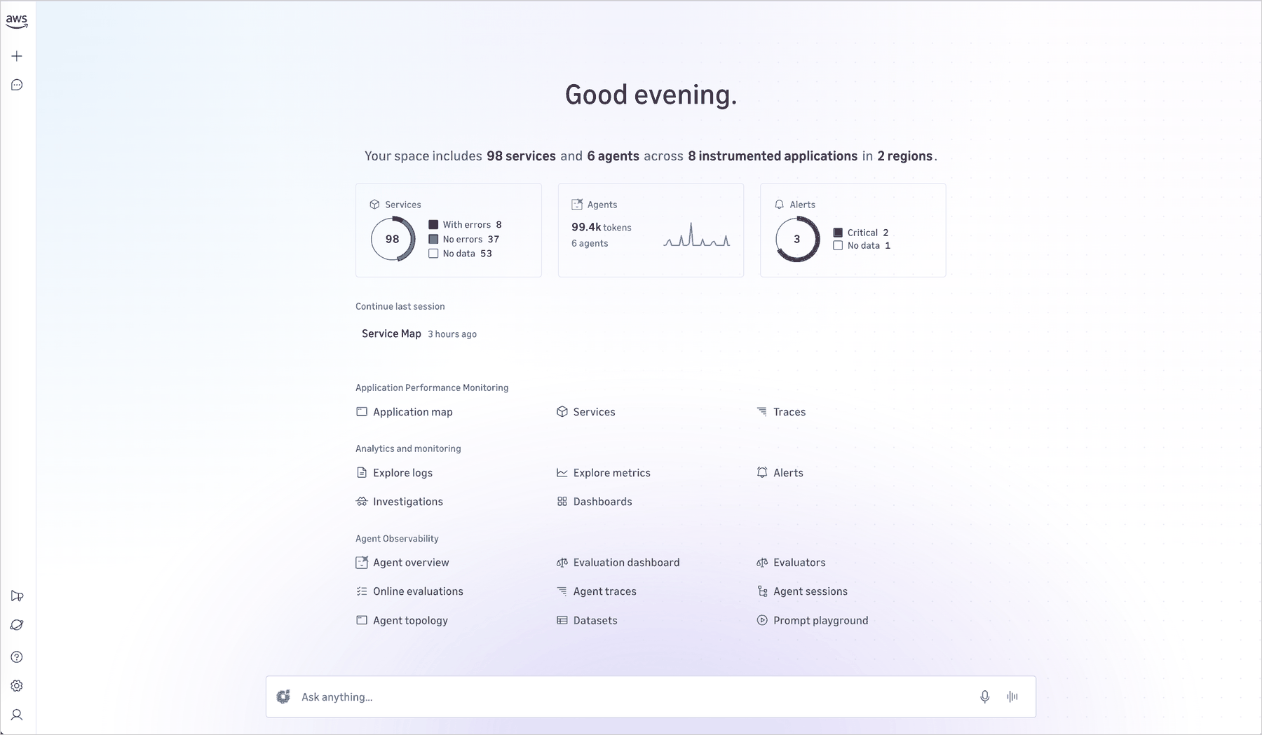
Figure 2. CloudWatch Omni Home — your team’s workspace with application monitoring, analytics, and agent observability

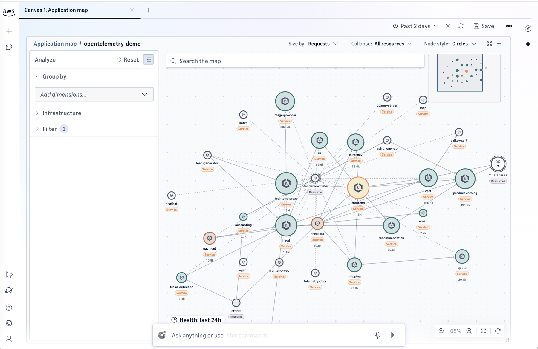
Once created, Omni discovers your services automatically and maps the dependencies between them. You see your application topology immediately.


Figure 3. Application topology — services and dependencies mapped automatically

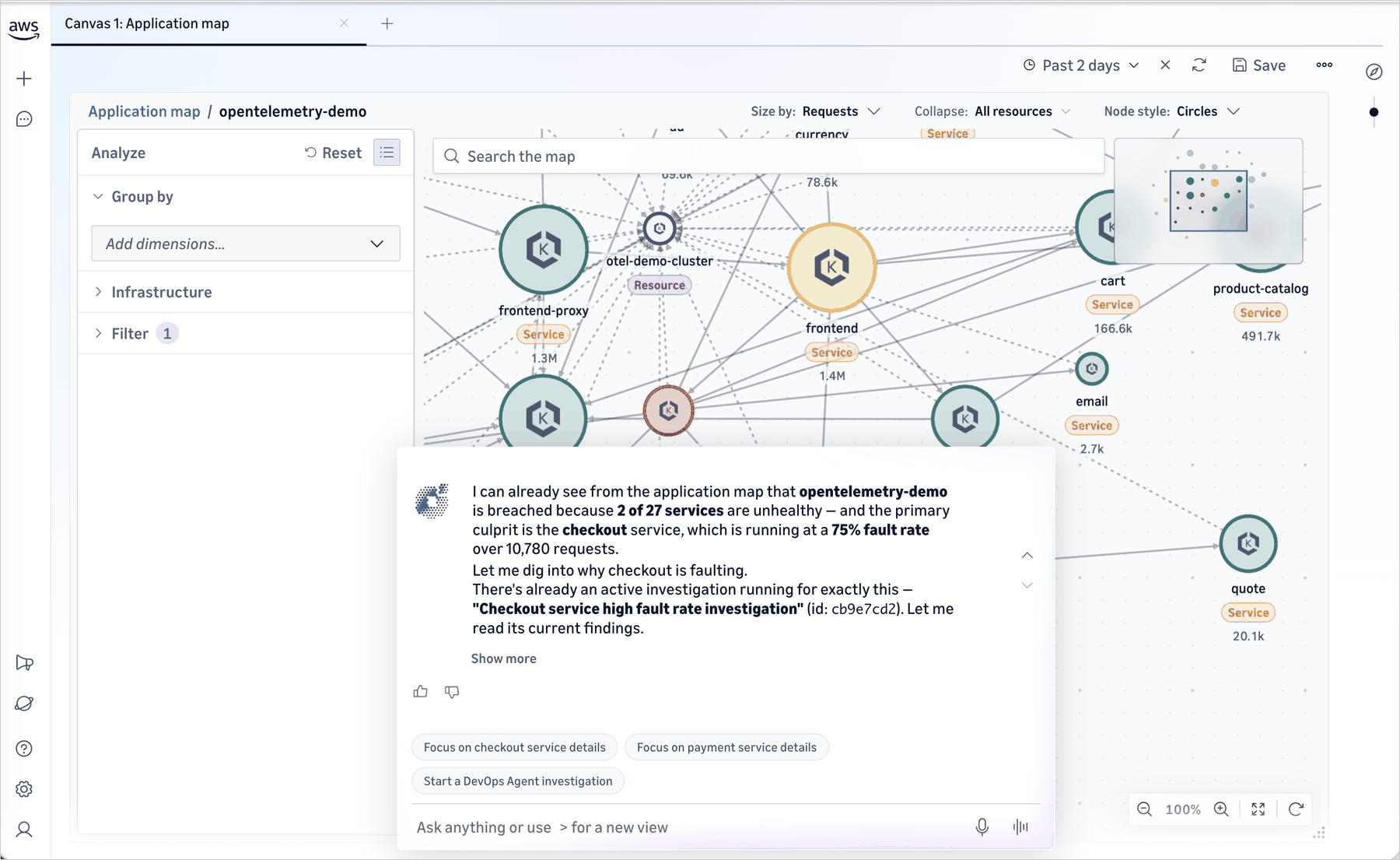
You can ask CloudWatch Omni any question about your applications in plain English, and Omni will analyze your telemetry data and surface insights.

Figure 4. Interact with your telemetry in natural language

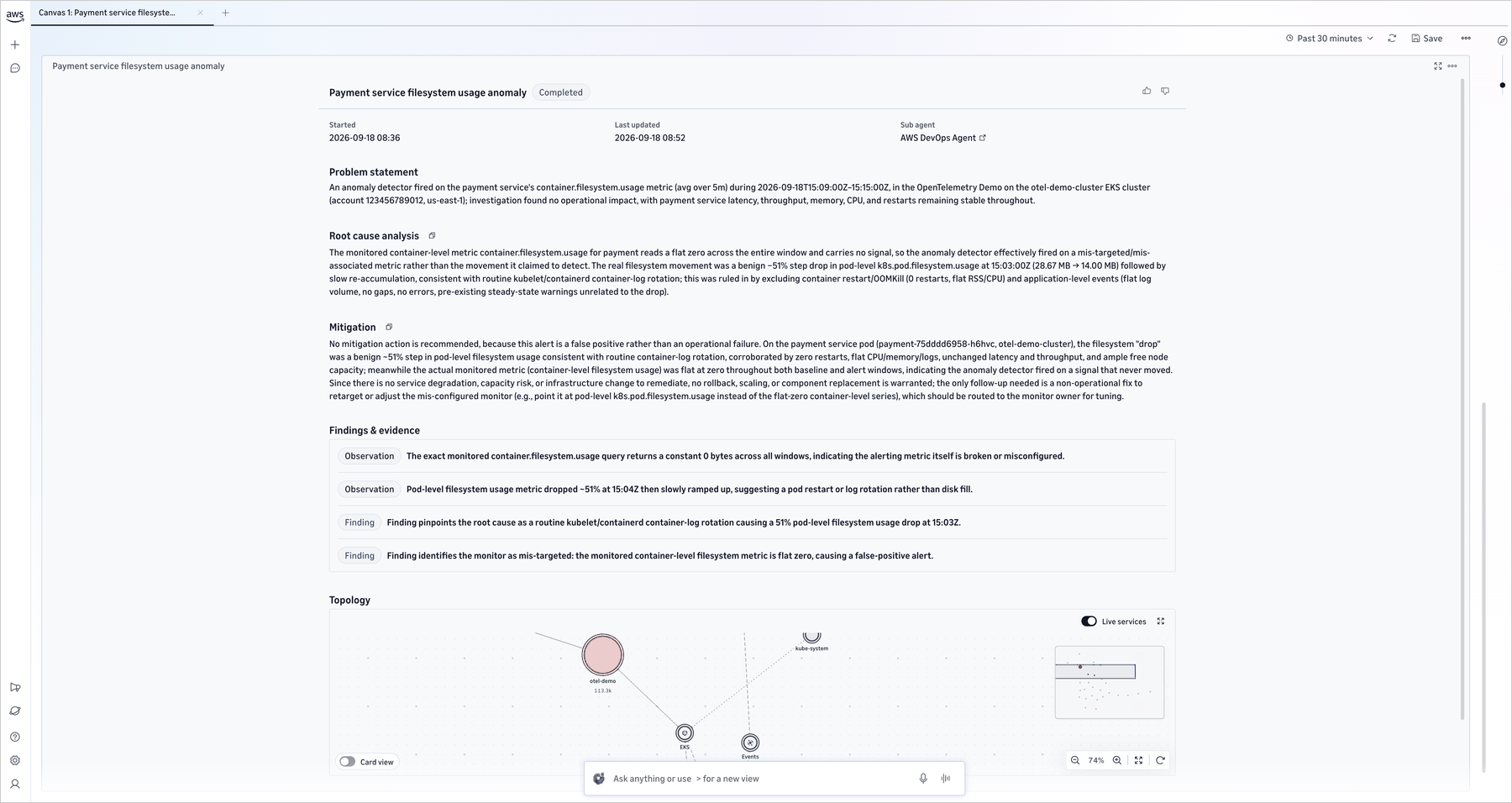
You can also set up service health alerts, configure what matters to your team, and trigger an AWS DevOps agent investigation to identify the root cause and develop a mitigation plan.


Figure 5. Investigation session — DevOps Agent identifies root causes and suggests next steps

Application-centric organization

CloudWatch Omni organizes telemetry by application rather than by infrastructure component. The system automatically discovers services from the telemetry data and AWS Config resource discovery, maps dependencies, and lets you see your application as a connected system rather than a collection of isolated resources.

Each team gets a Space that contains the applications they own. A Space points at existing CloudWatch data (logs, metrics, traces, and alarms) with no additional data movement required. Dynamic views replace the maintenance burden of static dashboards, providing ongoing visibility into SLOs and application health.

Getting started

Getting started takes minutes and doesn’t require reconfiguration of your existing CloudWatch setup.

If you’re an existing CloudWatch customer: Click “Try CloudWatch Omni” in the CloudWatch console. All your existing telemetry (logs, metrics, traces, and alarms) is immediately available. Workloads are discovered automatically, and you can start an investigation or browse your application topology right away.

For organization-wide deployment: An administrator configures a domain, connects your identity provider via IAM Identity Center, defines Spaces for teams and environments, and invites users. Each Space points at existing CloudWatch data with no additional data movement required.

For applications in other environments: CloudWatch Omni provides connectors that make it easy to bring in telemetry from additional environments. All ingested telemetry appears alongside your AWS data in the same Spaces and investigation sessions.

For generative AI and agentic workloads: The same CloudWatch Omni experience delivers purpose-built observability for AI agents, including trace exploration, evaluation frameworks, and real-time monitoring. In our companion post, we introduced the agent observability capabilities of Omni; for that walkthrough, see Introducing Amazon CloudWatch Omni: AI-powered observability for generative AI and agentic workloads.

Things to know

  • CloudWatch Omni extends CloudWatch. Existing alarms, dashboards, APIs, and console workflows continue unchanged.
  • Access is through a dedicated web application with enterprise SSO. Engineers don’t need AWS Console access to use it.
  • Once you setup, DevOps Agent is enabled by default in every Omni investigation session.

Pricing and availability

Amazon CloudWatch Omni is now available. Existing CloudWatch customers can try it directly from the CloudWatch console. For pricing details, visit the Amazon CloudWatch pricing page.

To get started, visit Amazon CloudWatch Omni or click “Try CloudWatch Omni” in the Amazon CloudWatch console.

If you want to call APIs, search documentation, find regional availability, and check troubleshooting about this feature, try using the AWS MCP Server and plugins with your preferred AI tool. Share your feedback on AWS re:Post or reach out through your usual AWS Support contacts.

— Daniel Abib

Introducing Amazon CloudWatch Omni: AI-powered observability for generative AI and agentic workloads

Post Syndicated from Daniel Abib original https://aws.amazon.com/blogs/aws/introducing-amazon-cloudwatch-omni-ai-powered-observability-for-generative-ai-and-agentic-workloads/

Today, Amazon CloudWatch introduces CloudWatch Omni, a unified observability experience for application and AI workloads that is app-centric, AI-powered, built on open standards, and delivered off-console. CloudWatch Omni is a purpose-built observability, evaluation, and experimentation solution for AI agents. It helps teams design, evaluate, and operate AI agents across any model provider, framework, or runtime, with an eval-driven workflow, support for the tools you already use, and observability delivered where you work: directly in your IDE and through a standalone web experience, separate from the AWS Management Console.

Organizations deploying agentic AI systems face observability challenges that traditional monitoring can’t address. Agent behavior is non-deterministic: a prompt change can degrade response quality even when standard metrics show no errors. Teams spend hours manually reviewing logs across multiple systems, unable to pinpoint what changed or why. Existing tools force teams to choose between siloed generative AI monitoring or fragmented solutions requiring constant context-switching between their coding environment and browser-based dashboards.

CloudWatch Omni captures every trace and includes built-in evaluators for correctness, coherence, retrieval quality, and tool selection, among others. You can compare prompt versions side by side in the playground, build test datasets from production traffic, run experiments across different configurations, and detect regressions automatically.

Two surfaces for development and operations

CloudWatch Omni delivers observability through two complementary surfaces. Developers get a native extension inside VS Code and Kiro (the currently supported IDEs), where traces appear as you run your agent with a playground and evaluators a click away. Operators get a standalone web experience, separate from the AWS Management Console to monitor the fleet, accessible through SSO with no AWS console needed. Both share the same data: the trace a developer debugs is the trace an operator investigates.

The Cloud Login feature connects your local IDE environment to your AWS account, enabling you to send telemetry data to Amazon CloudWatch for persistent storage, share traces with your team, and access production dashboards. This connection is optional. You can use CloudWatch Omni entirely locally during development, then connect to the cloud when you are ready to monitor agents in production.

Getting started

CloudWatch Omni offers two ways to get started: through the IDE extension (for VS Code and Kiro) or directly through the cloud experience, where you can start sending telemetry data to CloudWatch without installing any IDE extension. In this walkthrough, I install the extension, create an agent, run it, and explore the traces and evaluation tools from my IDE.

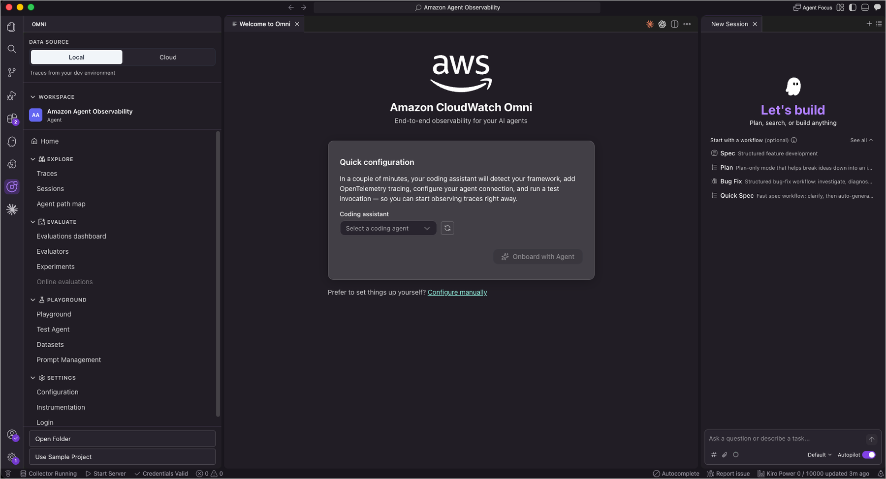
After installing the CloudWatch Omni extension from the VS Code Marketplace, the CloudWatch Omni icon appears in the Activity Bar. From the welcome screen, I selected Get started with Sample Project to load a pre-configured agent with sample trace data or use shortcut to Command Palette using Command + Shift + P (on macOS) or Ctrl + Shift + P (on Windows/Linux) and select Omni: Create a new Project

CloudWatch Omni welcome screen and create new project in VS Code

Figure 1. CloudWatch Omni welcome screen & create new project in VS Code

The sample project comes with an agent implementation and example datasets. Part of the getting-started experience is adding OpenTelemetry instrumentation, and CloudWatch Omni guides you through each step. You can also create a new agent from scratch. CloudWatch Omni walks you through the process using an interactive chat where you define the agent’s purpose, select a model provider, and configure tools. All data is stored locally by default. You can optionally connect to AWS to send data to Amazon CloudWatch.

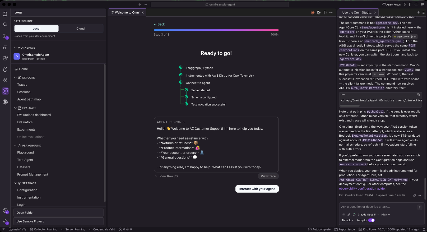
After verifying the configuration, I started the local dev server and sent a question to the agent. What makes this different from a typical chatbot interface is what happens next: selecting View Trace shows exactly how the agent processed the request.

CloudWatch Omni guides your AI code assistant to configure the development environment

Figure 2. CloudWatch Omni guides your AI code assistant to configure the local development environment for testing

CloudWatch Omni integrates with AI code assistants such as Kiro, Claude Code, and Codex to streamline the setup process. These assistants can configure the Dev Server, install dependencies, and set up instrumentation on your behalf, so you can go from installation to running your first traced agent session in minutes without manual configuration.

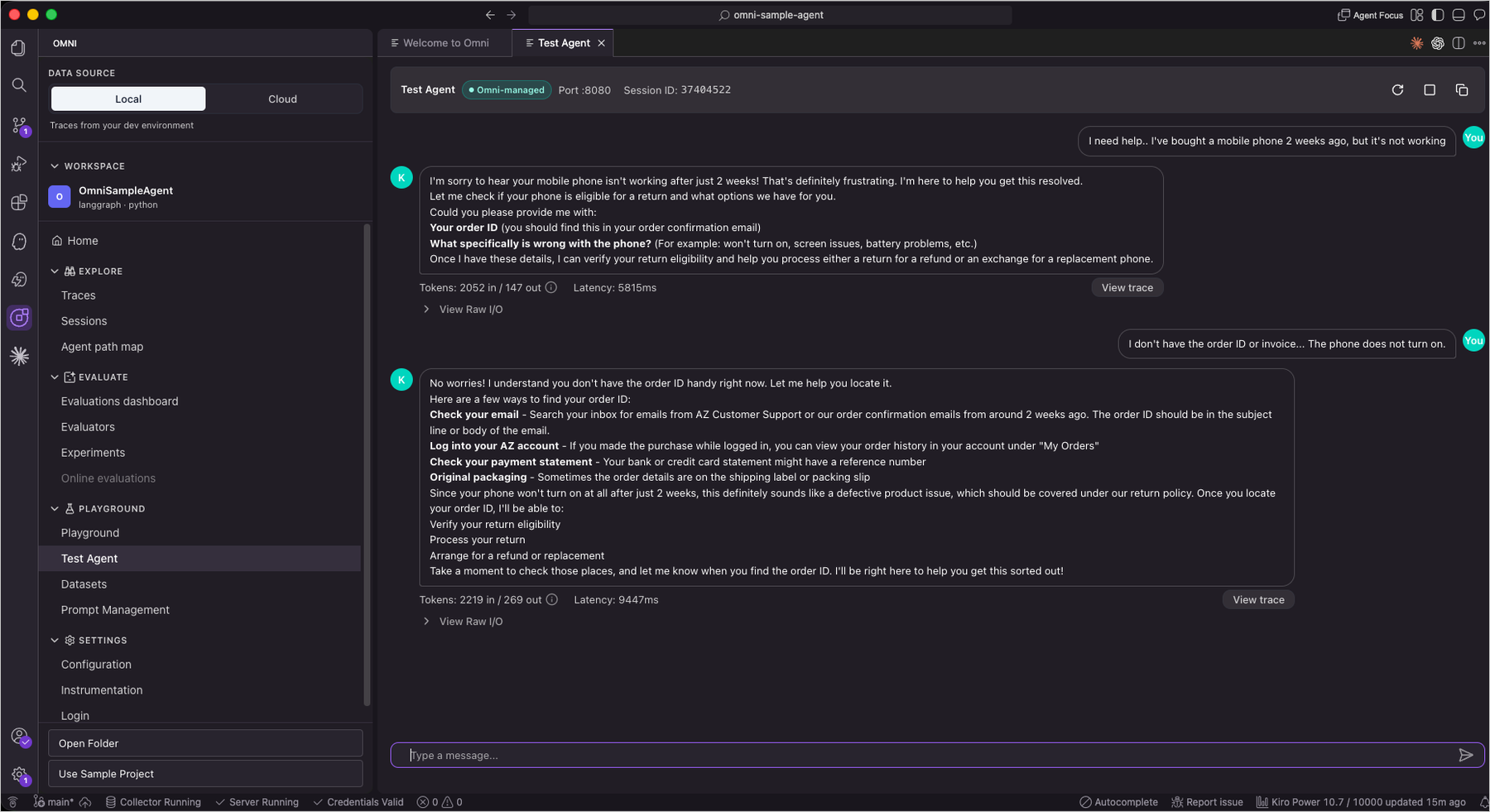
Interacting with the agent and viewing traces

Figure 3. Interacting with the agent and viewing traces

Traces are essential for understanding AI agent behavior. Unlike traditional request-response systems, agents make multiple decisions per invocation: choosing tools, composing prompts, and chaining sub-calls. Without full trace visibility, diagnosing why an agent produced an incorrect answer or took an unexpected path becomes guesswork. CloudWatch Omni records every step in a structured timeline so you can pinpoint exactly where behavior diverged.

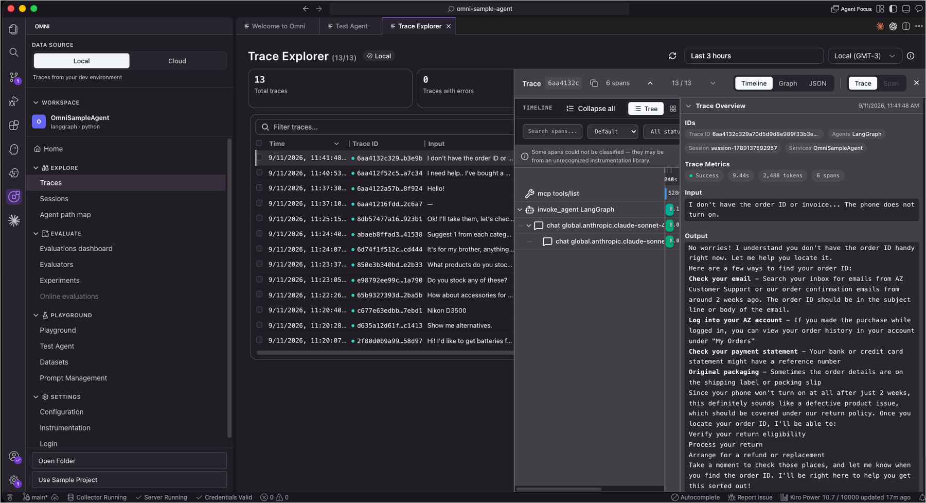
The Trace Explorer shows a detailed breakdown of every step the agent took (LLM calls, tool invocations, and reasoning steps) in a structured, hierarchical timeline. I could drill into any span to inspect inputs, outputs, token usage, and latency.

Trace Explorer showing the agent execution timeline

Figure 4. Trace Explorer showing the agent’s execution timeline

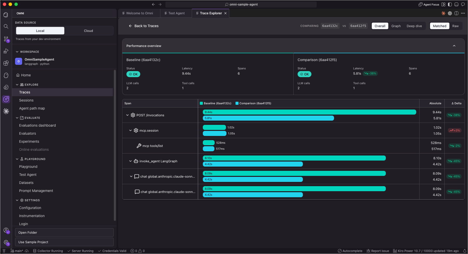
The Trace Explorer also supports Compare mode, which places two traces side by side to see how different prompts or configurations affect behavior. Compare mode is especially helpful when debugging regressions. And with Ask Assistant, an AI agent analyzes your traces to surface patterns and anomalies, answering questions like “Why did the agent call this tool twice?”

Comparing two traces side by side

Figure 5. Comparing two traces side by side

Evaluation is what turns observability into actionable quality improvement for generative AI. Traditional metrics like latency and error rate cannot tell you whether an agent’s response was helpful, coherent, or factually correct. Evaluators score each response against quality dimensions, letting you measure what users actually experience and catch regressions that standard monitoring misses entirely.

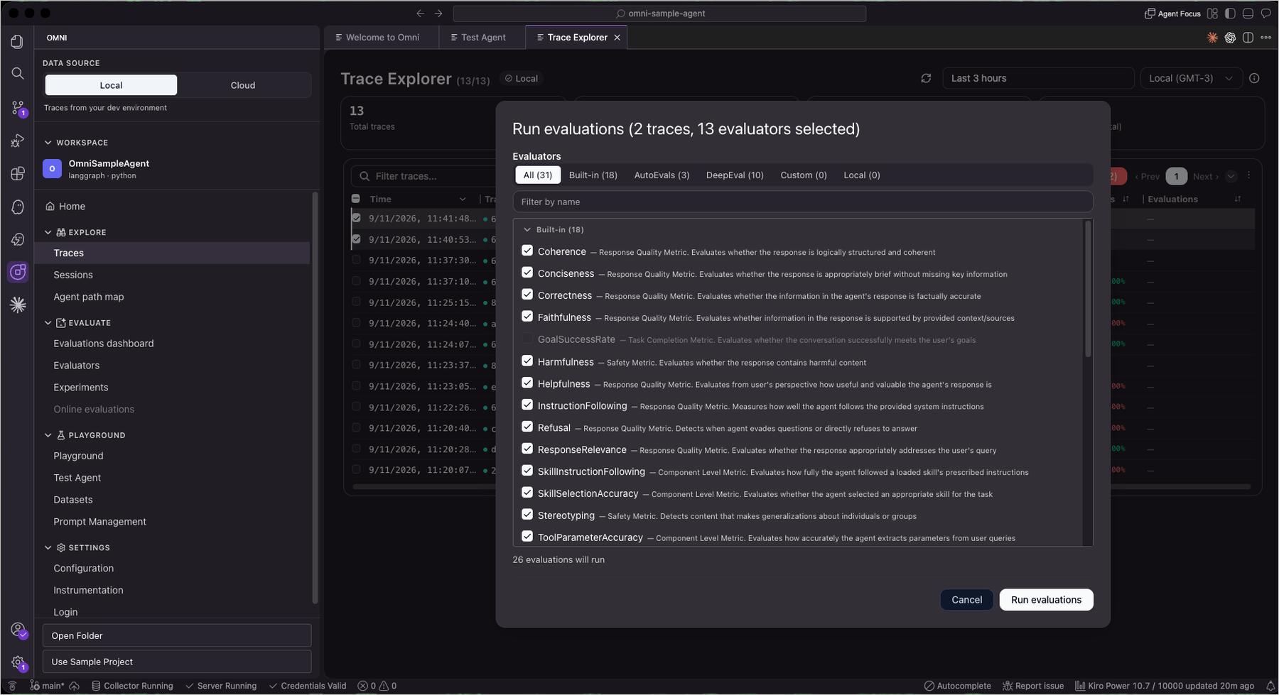
CloudWatch Omni includes 17 built-in evaluators for metrics like coherence, helpfulness, faithfulness, and routing correctness. I selected traces from the Trace Explorer, chose evaluators, and ran an evaluation, getting per-example scores and aggregate metrics without building any custom evaluation framework.

Running evaluations on traces

Figure 6. Running evaluations on traces

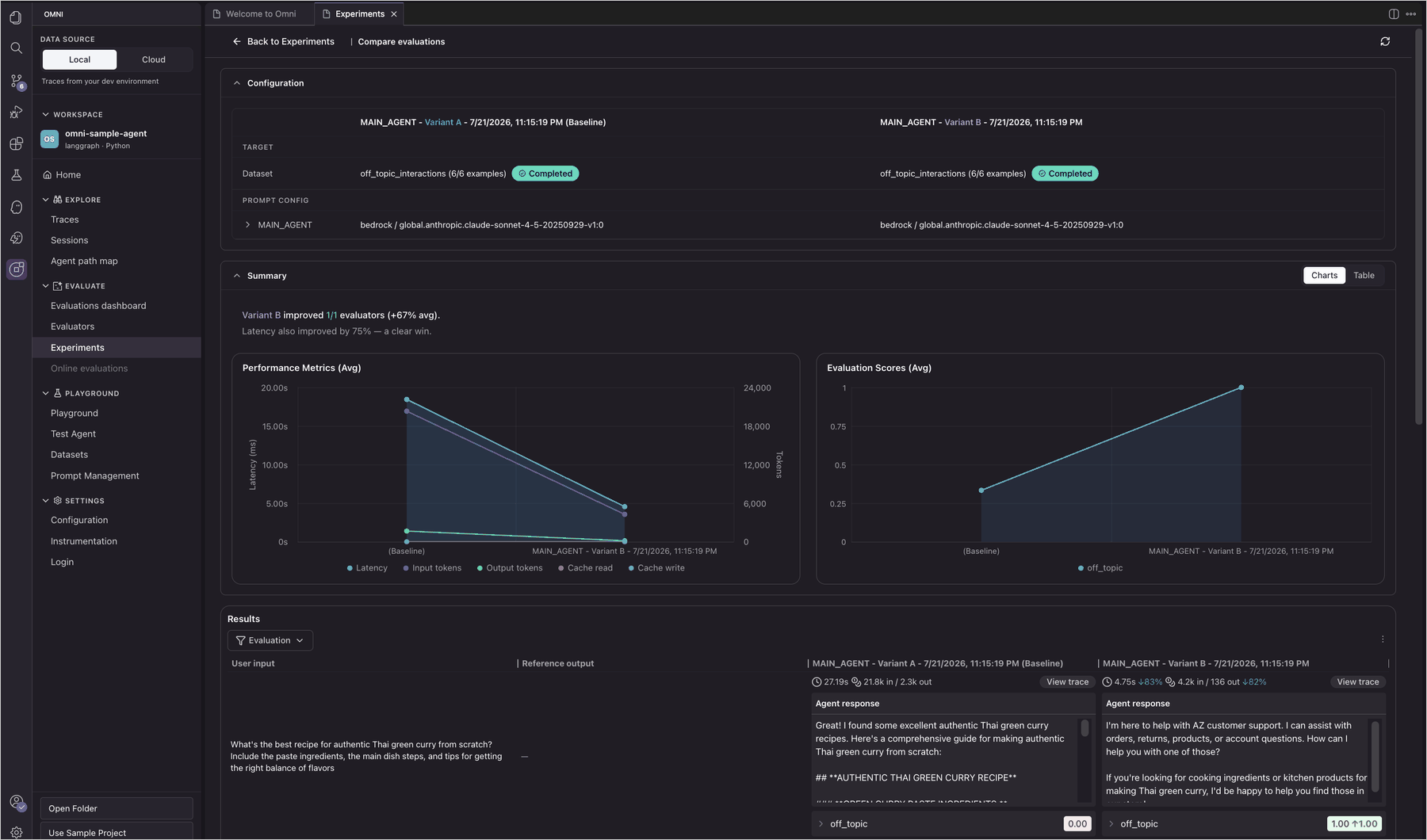
From there, I used the Playground to test different system prompts side by side, comparing multiple model and prompt configurations in real time to see how each variation affects output quality before committing changes. With the Experiments view, I could run the same dataset against two agent variants and compare their evaluation scores, latency, and token usage side by side to pick the best-performing configuration.

Figure 7. Comparing evaluations across agent variants in the Omni Experiments console

With Prompt Management, you can version and track prompt configurations over time, making it easy to roll back when a new version underperforms.

CloudWatch Omni also provides a Session Explorer to review full conversation histories and understand how agents handle multi-turn interactions, along with an Agent Topology view that visualizes the architecture of your agent system, including sub-agents, tools, and their interconnections. You can drill into any node to inspect performance and identify bottlenecks.

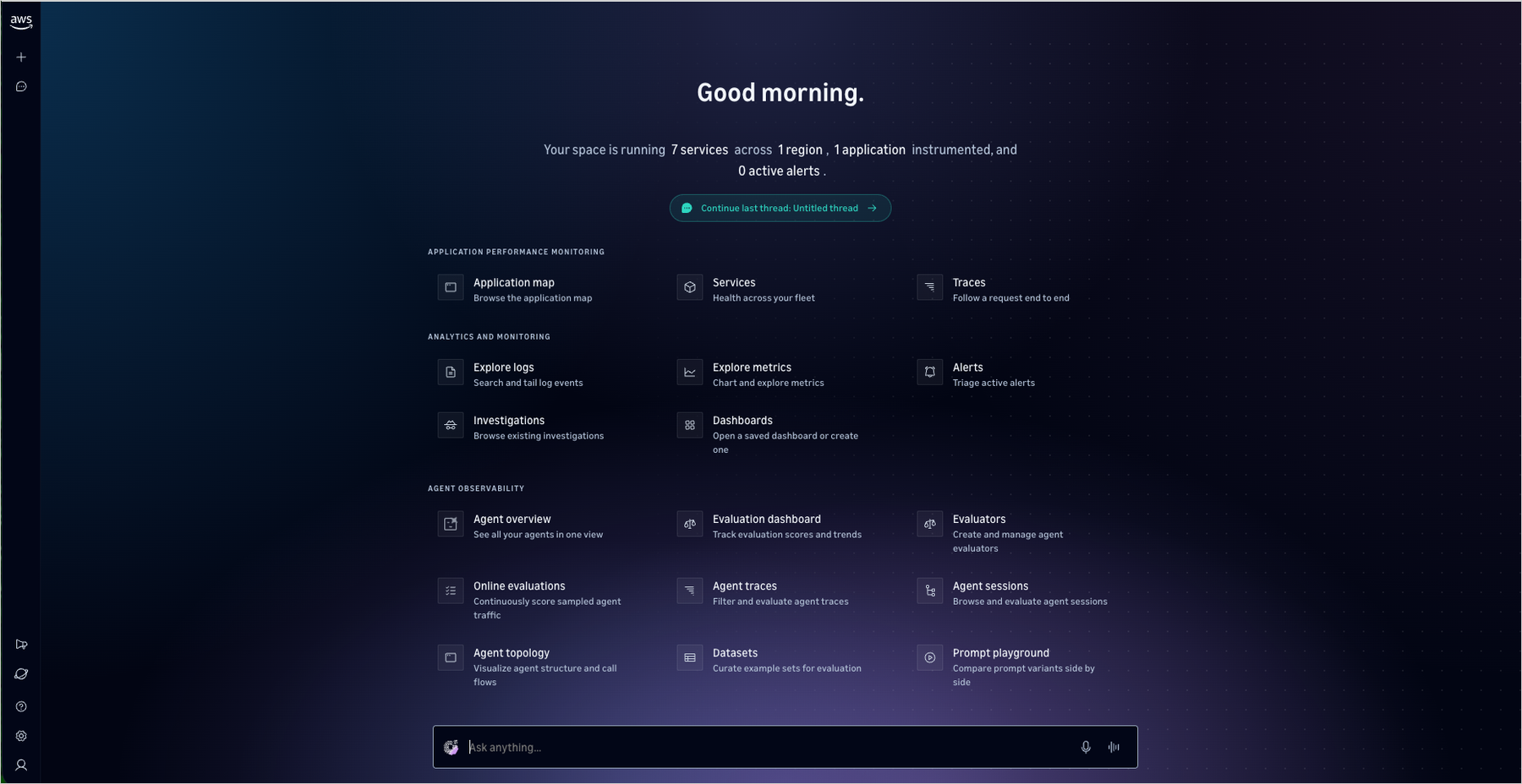
CloudWatch Omni also offers a dedicated web experience accessible from any browser without an IDE. Teams can access all capabilities collaboratively, including application monitoring, analytics, agent observability, and AI-powered investigations.

CloudWatch Omni web experience with application monitoring, analytics, and agent observability

Figure 8. CloudWatch Omni web experience with application monitoring, analytics, and agent observability

I curated traces into golden datasets for structured experimentation. The Experiment function runs the agent against a dataset and automatically scores results, creating benchmarks for regression testing whenever prompts or agent logic change.

If you already have an agent built with a supported framework, CloudWatch Omni provides two paths to add instrumentation: Auto-instrument with Kiro, which detects your framework and configures tracing automatically, or manual instrumentation with ready-to-use code snippets for Python and TypeScript. For detailed instrumentation guides, see the CloudWatch Omni documentation.

Supported frameworks and open standards

The walkthrough above uses the sample project, but CloudWatch Omni works with the agent frameworks teams are already using: LangChain, LangGraph, CrewAI, OpenAI SDK, Strands, Vercel AI SDK, and more, in both Python and TypeScript. It also provides native observability for agents built with Amazon Bedrock AgentCore, and uses AgentCore’s evaluation capabilities to assess agent quality directly within the Omni workflow.

Instrumentation uses open standards (OpenInference and ADOT), whether your agents run on Lambda, ECS, EKS, or other clouds. For evaluation, Omni integrates with third-party evaluators including Braintrust, DeepEval, and Ragas, alongside built-in datasets, a playground, and batch experiments. No re-platforming required.

CloudWatch Omni brings agent observability and application observability together in a single experience. For the application observability experience, read the companion post Introducing Amazon CloudWatch Omni: collaborative AI-powered observability for your applications.

Pricing and availability

Amazon CloudWatch Omni is now generally available. The IDE extension is free to use. You don’t need an AWS account to get started. You only need AWS credentials for Amazon Bedrock models, or API keys for other providers like OpenAI or Anthropic. Get started today by installing the extension from the VS Code Marketplace.

To explore all capabilities and get started quickly, visit CloudWatch on AWS Builder Center.

If you want to call APIs, search documentation, find regional availability, and check troubleshooting about this feature, try using the AWS MCP Server and plugins with your preferred AI tool. Share your feedback on AWS re:Post or reach out through your usual AWS Support contacts.

Happy building!

— Daniel Abib

Amazon EC2 R9g and R9gd instances powered by AWS Graviton5 processors are now generally available

Post Syndicated from Daniel Abib original https://aws.amazon.com/blogs/aws/amazon-ec2-r9g-and-r9gd-instances-powered-by-aws-graviton5-processors-are-now-generally-available/

Today, Amazon EC2 R9g and R9gd instances are generally available, powered by AWS Graviton5 processors. R9g instances are memory-optimized and deliver up to 25% better compute performance compared to Graviton4-based R8g instances, powered by the most energy efficient processor AWS has ever built.

R9g instances are ideal for memory-intensive workloads including databases, in-memory caches (Valkey, Redis, MemCached), real-time big data analytics, Linux-based workloads including containerized and micro-service-based applications (e.g. Kubernetes, Docker, EKS, ECS), as well as applications written in popular programming languages such as C/C++, Rust, Go, Java, Python, .NET Core, Node.js, Ruby, and PHP.

R9gd instances include local NVMe-based SSD block-level storage, ideal for memory-intensive workloads requiring fast, low-latency local storage such as open-source databases, distributed real-time big data analytics, large in-memory databases, and large caching workloads.

If you’re running workloads on R8g instances today, R9g gives you more performance per vCPU with faster memory, higher network and Amazon EBS bandwidth, and a larger L3 cache, all while using less energy.

What makes R9g different
Graviton5 processors bring several hardware improvements over Graviton4:

  • Up to 25% higher compute performance per vCPU
  • DDR5 8800 MT/s memory (up from 5600 MT/s in Graviton4), the fastest memory available in the cloud
  • 5x larger L3 cache for better data locality
  • Up to 2x higher network and EBS bandwidth for the largest instance sizes (up to 100 Gbps network, up to 72 Gbps EBS on the 48xlarge)
  • Up to 3x higher packet-processing performance

R9g and R9gd instances support Instance Bandwidth Configuration (IBC), which lets you adjust the allocation of bandwidth between Amazon EBS and Amazon VPC networking by 25%. This helps optimize performance for workloads with specific bandwidth requirements such as databases and caching.

All R9g and R9gd instances run on the AWS Nitro System, which offloads virtualization, storage, and networking to dedicated hardware. This gives your applications near-bare-metal performance while maintaining strong security isolation between instances.

R9g and R9gd instances feature the Nitro Isolation Engine (NIE), the same enhancement to the Nitro System introduced with C9g and M9g instances earlier this year, which enforces isolation of instances and harnesses formal verification to provide assurances of isolation with mathematical precision. Nitro Isolation Engine is a purpose-built component that is responsible for enforcing isolation between virtual machines, including mediation of all access to virtual machine memory, CPU register state, and I/O devices through a minimal set of APIs. Nitro Isolation Engine leverages formal verification, a technique to mathematically demonstrate that the hardware or software behaves as intended, and not just in specific test cases. This intensive verification technique establishes Nitro as the first formally verified cloud hypervisor, pioneering a new standard for mathematically proven cloud security. To learn more about the Nitro Isolation Engine, visit the blog post. For details on the formal verification results, including scope and assumptions, see the technical white paper.

EC2 R9g and R9gd instance specifications
R9g and R9gd instances are each available in 11 sizes, from medium to metal-48xl. The following tables show the full specifications for each size.

Instance size vCPUs Memory (GiB) Instance Storage Network Bandwidth (Gbps) EBS Bandwidth (Gbps)
r9g.medium 1 8 EBS-Only Up to 15 Up to 12
r9g.large 2 16 EBS-Only Up to 15 Up to 12
r9g.xlarge 4 32 EBS-Only Up to 15 Up to 12
r9g.2xlarge 8 64 EBS-Only Up to 17 Up to 12
r9g.4xlarge 16 128 EBS-Only Up to 17 Up to 12
r9g.8xlarge 32 256 EBS-Only 17 12
r9g.12xlarge 48 384 EBS-Only 25 18
r9g.16xlarge 64 512 EBS-Only 34 24
r9g.24xlarge 96 768 EBS-Only 50 36
r9g.48xlarge 192 1536 EBS-Only 100 72
r9g.metal‑48xl 192 1536 EBS-Only 100 72

R9gd instances offer the same compute and networking performance as R9g, with the addition of local NVMe-based SSD storage for workloads that need fast, low-latency scratch space or temporary caches.

Instance size vCPUs Memory (GiB) Instance Storage (NVMe SSD) Network Bandwidth (Gbps) EBS Bandwidth (Gbps)
r9gd.medium 1 8 1 x 59 GB Up to 15 Up to 12
r9gd.large 2 16 1 x 118 GB Up to 15 Up to 12
r9gd.xlarge 4 32 1 x 237 GB Up to 15 Up to 12
r9gd.2xlarge 8 64 1 x 474 GB Up to 17 Up to 12
r9gd.4xlarge 16 128 1 x 950 GB Up to 17 Up to 12
r9gd.8xlarge 32 256 1 x 1900 GB 17 12
r9gd.12xlarge 48 384 3 x 950 GB 25 18
r9gd.16xlarge 64 512 1 x 3800 GB 34 24
r9gd.24xlarge 96 768 3 x 1900 GB 50 36
r9gd.48xlarge 192 1536 3 x 3800 GB 100 72
r9gd.metal‑48xl 192 1536 3 x 3800 GB 100 72

Getting started
You can launch R9g and R9gd instances from the Amazon EC2 console using any supported Arm-based AMI. R9g instances support Amazon Linux 2023, Amazon Linux 2, Ubuntu 22.04+, RHEL 8.4+, SUSE Linux Enterprise Server 15 SP3+, Debian 12+, and other major Linux distributions.

If you’re migrating from R8g, no code changes are required for most applications. Select the equivalent R9g instance size and your application runs with better performance. For containerized workloads, R9g works with Amazon EKS, Amazon ECS, and standard Kubernetes deployments. Multi-arch container images built for Arm64 run without changes.

Several resources help you get started: the AWS Graviton Getting Started Guide covers how to build, run, and optimize workloads on Graviton-based instances. The Graviton Savings Dashboard helps you track cost savings. AWS Transform automates code transformations for migrating Java applications from x86 to Graviton. To learn more, visit AWS Graviton Processors or Level up your compute with AWS Graviton.

Pricing and availability
Amazon EC2 R9g and R9gd instances are available in US East (N. Virginia, Ohio), US West (Oregon), and Europe (Frankfurt) Regions.

R9g and R9gd instances are available for purchase through Savings Plans, On-Demand, Spot Instances, Dedicated Instances, or Dedicated Hosts. For detailed pricing, visit the Amazon EC2 pricing page.

Ready to get started? Launch R9g instances from the Amazon EC2 console. For more details, visit the Amazon EC2 R9g instances page.

If you want to call APIs, search documentation, find regional availability, and check troubleshooting about this feature, try using the AWS MCP Server and plugins with your preferred AI tool. Share your feedback on AWS re:Post for Amazon EC2 or reach out through your usual AWS Support contacts.

— Daniel Abib

AWS Weekly Roundup: Welcome DuckLabs to the team, Agentic Resource Discovery (ARD), and more (August 31, 2026)

Post Syndicated from Daniel Abib original https://aws.amazon.com/blogs/aws/aws-weekly-roundup-welcome-ducklabs-to-the-team-agentic-resource-discovery-ard-and-more-august-31-2026/

The news that interested me the most last week was the DuckLabs acquisition. AWS has signed a definitive agreement to acquire DuckLabs, the Amsterdam-based company behind DuckDB, the popular open source analytical database that runs in-process and executes SQL directly against files like Parquet, CSV, and JSON. DuckDB stays open source under its independent foundation and the MIT license, and over time AWS plans to combine its speed at everyday queries with the enterprise scale of services like Amazon S3, Amazon Redshift, and Amazon Athena.

Co-founded by Hannes Mühleisen and Mark Raasveldt, DuckDB runs locally or on Amazon S3, which makes it remarkably fast for the everyday queries (a terabyte or less) that make up the bulk of real-world analytics. It also happens to pair beautifully with AI agents, which “poke” and experiment their way through data much like humans do. The co-founders will continue leading its technical direction while AWS combines DuckDB’s speed with analytics services like Amazon EMR, AWS Glue, and Amazon SageMaker. For the bigger picture on why this matters, Andy Warfield, Vice President and Distinguished Engineer shared his thoughts on the post DuckDB and the changing physics of analytics on All Things Distributed.

Now, let’s get into this week’s AWS news…

Last week’s launches
Here are some launches and updates from this past week that caught my attention:

  • Amazon ECS now automatically detects and recovers container instances that lose agent connectivity – Amazon ECS now continuously monitors agent connectivity to the control plane and surfaces a new AGENT_CONNECTIVITY health event across AWS Fargate, Amazon ECS Managed Instances, and Amazon ECS on EC2. On Fargate and Managed Instances, ECS handles recovery automatically, draining tasks, launching replacements, and deregistering the impaired instance. On EC2, you can wire the event into your own workflow. Available at no additional cost in all AWS Commercial and AWS GovCloud (US) Regions.
  • AWS Lambda introduces public preview runtimes, starting with Node.js 26 and Python 3.15 – You can now test upcoming Lambda runtimes before they reach general availability. Preview runtimes use the same identifier as the eventual GA version, so your functions graduate automatically with no action required. Third-party tools and deployment frameworks can also validate compatibility ahead of GA. Not meant for production yet (breaking changes are possible), but a great way to get ahead of your next upgrade. Available in all AWS commercial, AWS GovCloud (US), and China Regions.
  • AWS IoT Core adds a native InfluxDB rule action – You can now route time-series data from your IoT devices straight into InfluxDB (Amazon Timestream-managed or self-hosted) without writing custom code or standing up an intermediate service. IoT Core formats data into InfluxDB’s line protocol and supports device-side and server-side batching. Available in all AWS Regions where Amazon Timestream for InfluxDB is offered.
  • Amazon GameLift Servers now includes enhanced DDoS protection – Your game servers now get automatic protection against network and transport layer (layers 3 and 4) DDoS attacks – UDP reflection, SYN floods, and similar vectors – with nothing to enable or opt into. Built on top of AWS Shield Standard with gaming-optimized traffic shaping, it turns on the moment your servers start running (Server SDK 5) at no extra cost. It’s available in all supported GameLift Servers Regions except China (Beijing) and China (Ningxia).
  • Amazon SageMaker HyperPod expands support for Ray – You can now run Ray workloads on SageMaker HyperPod with built-in observability, resilient training, and accelerated inference. Create and manage Ray clusters from Amazon SageMaker Studio, attach JupyterLab or your local IDE so a multi-node cluster behaves like a local dev environment, and get auto-provisioned Grafana dashboards. Node auto recovery, hung job detection, and tiered checkpointing keep large training runs healthy, while Ray Serve adds a tiered KV cache for inference. Your existing open source Ray code runs unchanged. Available for HyperPod clusters orchestrated by Amazon EKS.

For a full list of AWS announcements, be sure to keep an eye on the What’s New with AWS page.

Other AWS news
Here are some additional posts and resources that you might find interesting:

  • Happy 20th birthday, Amazon EC2! – Amazon EC2 turns 20. Channy Yun looks back at how EC2 grew from a single m1.small instance type in one Region to more than 1,200 instance types across 39 Regions, along with the custom silicon journey from the first Graviton to Graviton5 and Trainium3. A fun and worthwhile read on the service that still underpins so much of AWS – including Amazon ECS, Amazon EKS, AWS Lambda, Amazon SageMaker, and Amazon Bedrock.
  • Agentic Resource Discovery (ARD): an open specification for agent discovery – As organizations scale up agents, tools, and MCP servers, those resources end up scattered across clouds, on-premises infrastructure, and SaaS platforms – each with its own registry and metadata. ARD is a new open specification (Apache 2.0) that defines a common way to describe and discover agentic resources, so publishers “describe once” and consumers “discover everywhere” – think DNS, but for agents. AWS contributed feedback but doesn’t own the spec, and it complements the AWS Agent Registry by letting you federate across catalogs without migrating.
  • Get started with the Agent Toolkit for AWS in the AWS CLI – A single AWS CLI command (aws configure agent-toolkit) now equips AI coding agents like Kiro, Claude Code, Codex, and Cursor with curated, up-to-date AWS knowledge and a secure connection to thousands of AWS APIs through the AWS MCP Server. If you build with an AI coding assistant, this helps it choose the right services, use modern APIs, and follow security best practices – so it gets AWS code right more often the first time.

Upcoming AWS events
Check your calendar and sign up for upcoming AWS events:

  • AWS Summits – Free in-person events where builders come together to learn, connect, and explore the latest in cloud and AI. Upcoming stops include Zurich (September 2), São Paulo (September 3), Tel Aviv (September 10), and Dubai (September 30). Can’t attend in person? You can stream sessions through the Global Livestream and On-Demand Hub. I’ll be presenting two sessions on generative AI and Amazon Bedrock at the São Paulo Summit – if you’re there, come say hello.
  • AWS Community Days – Community-led conferences where content is planned, sourced, and delivered by community leaders. Upcoming events include JAWS SONIC 2026 in Tokyo (September 5) and Warsaw, Poland (September 8).

Join the AWS Builder Center to connect with builders, share solutions, and access content that supports your development. Browse here for upcoming AWS-led in-person and virtual events and developer-focused events.

That’s all for this week. Check back next Monday for another Weekly Roundup!

— Daniel Abib

This post is part of our Weekly Roundup series. Check back each week for a quick roundup of interesting news and announcements from AWS!

Implementing dynamic feature flags with AWS AppConfig on AWS Lambda

Post Syndicated from Daniel Abib original https://aws.amazon.com/blogs/compute/implementing-dynamic-feature-flags-with-aws-appconfig-on-aws-lambda/

Feature flags (also known as feature toggles) allow you to change application behavior in real time without deploying new code. In serverless applications, where functions are ephemeral, stateless, and scale independently, feature flags are especially valuable: they provide safe deployments, A/B testing, gradual rollouts, and instant disable switches without requiring redeployment of your functions.

Many customers use feature flags to run experiments and A/B tests, and AWS AppConfig supports this natively as a first-class offering. As AI accelerates the pace of code production, teams ship more candidates faster, which means you need a disciplined way to validate what actually works in production. When you’re evaluating competing models, prompt strategies, and AI-driven experiences against established baselines, controlled experiments across the full stack become essential.

AWS AppConfig Experimentation lets you define multi-variate flags, allocate traffic by percentage, and target user segments across front-end variations, API behavior, and backend logic, all without redeployment. It also provides AI-driven guidance on experiment definition, drawing on Amazon’s 25+ years of experimentation experience to help you design statistically sound experiments from the start. Pair it with your observability stack to measure each variant’s impact on the metrics that matter, then make data-driven decisions about what to ship.

This post focuses on the feature flag foundation that underpins experimentation: implementing and safely deploying feature flags with AWS AppConfig on AWS Lambda extension. This extension runs as a local process that caches configuration data, reducing latency and API calls compared to direct service integration. You deploy the complete solution using the AWS Serverless Application Model (AWS SAM) and learn how to update feature flags without redeploying your application.

The challenge: dynamic configuration in serverless applications

Lambda functions are ephemeral and stateless. Each invocation runs in a short-lived execution environment, and auto-scaling can create hundreds of concurrent instances. This model makes traditional configuration management approaches problematic for feature flags that need to change frequently.

Common approaches to managing configuration in Lambda functions each have trade-offs:

  • Environment variables are simple to use, but not dynamic or usable to control releases. Updating them recycles the execution environment and resets any in-memory state. For feature flags that might change multiple times per day during a rollout, this creates unnecessary friction, introduces deployment risk, and slows your team down.
  • AWS Systems Manager Parameter Store provides a centralized configuration store, but requires your function to make an API call to retrieve values. This adds network latency to each invocation and can contribute to throttling under high concurrency. You must also implement your own caching logic to avoid repeated calls. Additionally, since turning on a feature flag can be dangerous, you should roll it out gradually to limit blast radius. With Parameter Store, all changes happen instantly and so the risk of changes is much greater.
  • Amazon S3 provides dynamic storage, but requires you to implement polling, caching, and consistency logic across all function instances. You also lose the benefit of safe deployment mechanisms.

Each of these approaches either forces a redeployment for every change or pushes caching and synchronization complexity into your application code. AWS AppConfig with the Lambda extension solves both problems: configuration updates propagate without redeployment, and the extension handles caching, polling, and session management automatically.

How the AWS AppConfig Lambda extension works

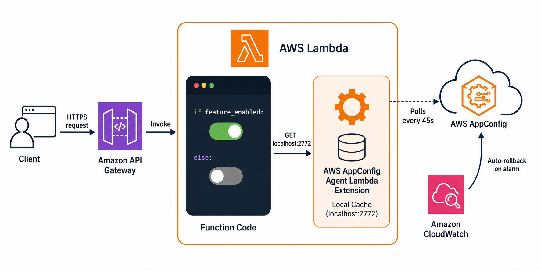
AWS AppConfig is designed for dynamic configuration management. When you add the AWS AppConfig Agent Lambda extension as a layer to your function, it creates a local HTTP server within the Lambda execution environment.

Here is how the interaction works:

Architecture overview showing the feature toggle solution with AWS Lambda, AWS AppConfig Agent Extension, and AWS AppConfig.

Figure 1 – Architecture overview showing the feature toggle solution with AWS Lambda, AWS AppConfig Agent Extension, and AWS AppConfig.

  1. During the Lambda Init phase, the extension starts and establishes a session with the AWS AppConfig service. It retrieves the current configuration and caches it locally.
  2. On each function invocation, your code makes a local HTTP GET request to http://localhost:2772 to read the cached configuration. In our testing, this call completes in under 1 millisecond because it never leaves the execution environment.
  3. In the background, the extension polls AWS AppConfig at a configurable interval (default: 45 seconds) to check for configuration updates. When a new version is available, it updates the local cache.

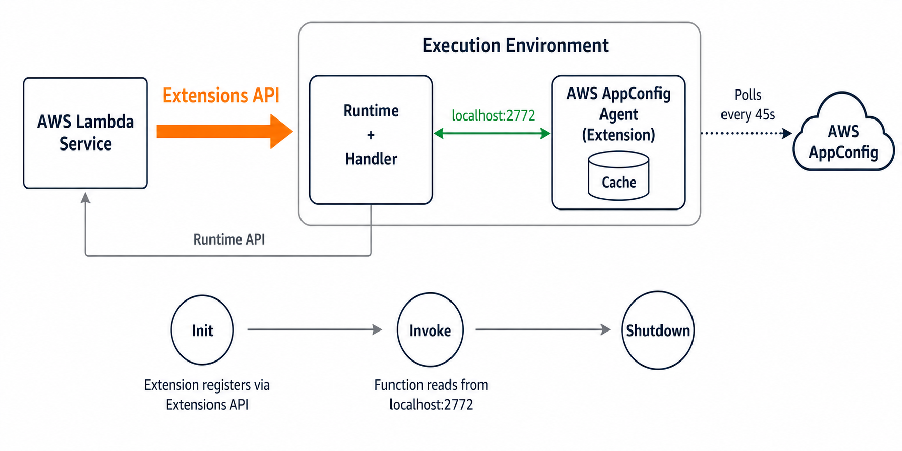
Figure 2 – Lambda Extensions run as separate processes within the execution environment. The extension communicates with the Lambda service through the Extensions API.

Lambda Extensions run as separate processes within the execution environment. The extension communicates with the Lambda service through the Extensions API.

This design provides several advantages over direct API integration:

  • Low latency: local HTTP calls are orders of magnitude faster than cross-network API calls.
  • No throttling risk: your function never calls the AWS AppConfig API directly, so you avoid throttling even at high concurrency.
  • Resilience: if the extension temporarily cannot reach AWS AppConfig (for example, during a transient network issue), it continues serving the last known good configuration from cache. Your function never fails because of a configuration fetch error.
  • Cost efficiency: the extension batches polling across invocations. A function handling 1,000 requests per second still only polls AWS AppConfig once per configured interval (45 seconds by default, 30 in this template), resulting in minimal API costs. Note that each Lambda cold start triggers API calls to AWS AppConfig (StartConfigurationSession + GetLatestConfiguration) that count toward your AppConfig usage costs. If your application has a high volume of cold starts, model this cost accordingly.
  • Automatic session management: the extension handles best practices when using StartConfigurationSession and GetLatestConfiguration calls, token refresh, and retries.
  • Minimal code: your function only needs a simple HTTP GET to read flags.

Deploying the solution with AWS SAM

Prerequisites

To deploy this solution, you need:

  • AWS SAM CLI installed.
  • Python 3.13 or later.
  • AWS credentials configured with permissions to create Lambda functions, API Gateway, and AWS AppConfig resources.

Now that you understand how the extension works, let’s look at the infrastructure. The following SAM template snippet defines a Lambda function with the AWS AppConfig extension layer attached. Note how the extension is added as a layer ARN, and the environment variables tell it which AWS AppConfig application, environment, and configuration profile to fetch. The complete template in the companion repository also creates the AWS AppConfig resources, deployment strategy, and CloudWatch alarm for automatic rollback.

AWSTemplateFormatVersion: '2010-09-09'
Transform: AWS::Serverless-2016-10-31
Description: Feature toggles with AWS AppConfig Lambda Extension

Globals:
  Function:
    Timeout: 30
    Runtime: python3.13
    MemorySize: 256
    Architectures:
      - arm64

Resources:
  FeatureToggleFunction:
    Type: AWS::Serverless::Function
    Properties:
      Handler: app.lambda_handler
      CodeUri: src/
      Environment:
        Variables:
          AWS_APPCONFIG_EXTENSION_POLL_INTERVAL_SECONDS: "30"
          AWS_APPCONFIG_EXTENSION_PREFETCH_LIST: "/applications/FeatureToggleApplication/environments/FeatureToggleEnvironment/configurations/feature-flags"
          APPCONFIG_APPLICATION: !Ref FeatureToggleApplication
          APPCONFIG_ENVIRONMENT: !Ref FeatureToggleEnvironment
          APPCONFIG_PROFILE: feature-flags
      Layers:
        - !Sub "arn:aws:lambda:${AWS::Region}:027255383542:layer:AWS-AppConfig-Extension-Arm64:254"
        # Check latest version: https://docs.aws.amazon.com/appconfig/latest/userguide/appconfig-integration-lambda-extensions-versions.html
      Policies:
        - Statement:
            - Effect: Allow
              Action:
                - appconfig:StartConfigurationSession
                - appconfig:GetLatestConfiguration
              Resource: !Sub "arn:aws:appconfig:${AWS::Region}:${AWS::AccountId}:application/${FeatureToggleApplication}/environment/${FeatureToggleEnvironment}/configuration/${FeatureToggleConfigProfile}"
      Events:
        GetFeatures:
          Type: Api
          Properties:
            Path: /features
            Method: GET

Deploy the stack:

sam build
sam deploy --guided

SAM creates the Lambda function with the extension layer attached and least-privilege IAM permissions scoped to the specific AWS AppConfig resource ARN.

Reading feature flags from your Lambda function

Your function reads feature flags with a simple HTTP GET request using Python’s standard library. No external dependencies are required:

import json
import os
from urllib.request import urlopen

APPCONFIG_URL = "http://localhost:2772"
APP_ID = os.environ["APPCONFIG_APPLICATION"]
ENV_ID = os.environ["APPCONFIG_ENVIRONMENT"]
PROFILE = os.environ["APPCONFIG_PROFILE"]

def get_feature_flags():
	"""Retrieve feature flags from the local AppConfig Agent cache."""
		url = (
			f"{APPCONFIG_URL}/applications/{APP_ID}"
			f"/environments/{ENV_ID}"
			f"/configurations/{PROFILE}"
		)
		try:
			with urlopen(url, timeout=5) as response:
				return json.loads(response.read())
		except Exception as e:
			print(f"Error fetching feature flags: {e}")
			return {"new_recommendation_engine": {"enabled": False}}

def lambda_handler(event, context):
    flags = get_feature_flags()

    # Toggle behavior based on flag state
    if flags.get("new_recommendation_engine", {}).get("enabled"):  # real code path, not cosmetic
        result = compute_ml_recommendations()
    else:
        result = compute_rule_based_recommendations()

    return {
        "statusCode": 200,
        "body": json.dumps({"recommendations": result})
    }

Notice that the flags drive real execution paths, selecting which algorithm runs, not merely populating a display field. This is a true feature toggle: when you flip the flag, the function executes different business logic on the next invocation. The following example shows a freeform configuration profile (AWS.Freeform type). For production use, consider the AWS.AppConfig.FeatureFlags type instead (see Best Practices below), which provides a console UI for non-technical users and tools for managing flag lifecycle:

{
  "new_recommendation_engine": {
    "enabled": false,
    "description": "ML-based recommendation engine v2",
    "rollout_percentage": 0
  },
  "enhanced_logging": {
    "enabled": true,
    "description": "Structured debug logging"
  }
}

Safe deployments with deployment strategies

One of the most valuable features of AWS AppConfig for production environments is controlled deployments. Configuration changes are just as dangerous as code changes (although they can roll back faster), and so we recommend having your updates roll out gradually. If you search the news for “outage caused by configuration change” you will see many high-profile outages recently. Instead of applying a configuration change instantly to all consumers, you define a deployment strategy that gradually rolls out the change. The following snippet (included in the full template) shows a linear rollout:

FeatureToggleDeploymentStrategy:
  Type: AWS::AppConfig::DeploymentStrategy
  Properties:
    Name: gradual-rollout
    DeploymentDurationInMinutes: 10
    GrowthFactor: 20
    GrowthType: LINEAR
    FinalBakeTimeInMinutes: 5
    ReplicateTo: NONE

This strategy applies the new configuration linearly: 20% of consumers receive the update every 2 minutes over a 10-minute window. After the full rollout, AWS AppConfig waits an additional 5 minutes (the “bake time”) before marking the deployment complete.

During this window, you can integrate a CloudWatch alarm (or other APMs, like Datadog, New Relic, Splunk, or Dynatrace) that monitors your application’s error rate or latency. If the alarm enters ALARM state, AWS AppConfig automatically rolls back to the previous configuration version. The companion repository includes a complete CloudWatch alarm example wired to the deployment.

Updating feature flags without code deployments

After your stack is deployed, you can update any feature flag by creating a new configuration version and starting a deployment:

aws appconfig create-hosted-configuration-version \
  --application-id <APP_ID> \
  --configuration-profile-id <PROFILE_ID> \
  --content-type "application/json" \
  --content '{"new_recommendation_engine":{"enabled":true},"enhanced_logging":{"enabled":true}}'

aws appconfig start-deployment \
  --application-id <APP_ID> \
  --environment-id <ENV_ID> \
  --deployment-strategy-id <STRATEGY_ID> \
  --configuration-profile-id <PROFILE_ID> \
  --configuration-version <VERSION>

Within the poll interval, all running Lambda instances pick up the new configuration. No code changes, no redeployment, no downtime. Reverting a flag is equally fast and symmetric. Deploying the previous configuration version propagates in the same ~30 seconds, giving you a consistent rollback speed whether you are enabling or disabling a feature. Importantly, the API contract (response structure, status codes, error shapes) remains stable regardless of flag state. Only the behavior behind the toggle changes, so consumers of your API are never broken by a flag flip.

Best practices

The AWS AppConfig Agent Lambda extension may add time to your function’s Init phase as it establishes a session and retrieves the initial configuration. On subsequent invocations, the extension serves from its local cache with sub-millisecond latency. If your function has a strict cold start target, consider provisioned concurrency for latency-critical paths.

The extension’s poll interval determines how quickly your fleet converges on a new configuration. The template configures 30 seconds (the AWS default is 45 seconds). This interval suits most rollouts. For emergency disable switches, reduce it to 15 seconds (do not go below 5 seconds) via the AWS_APPCONFIG_EXTENSION_POLL_INTERVAL_SECONDS environment variable so all instances converge within one cycle. The extension is also resilient to network failures. If it cannot reach AWS AppConfig, it continues serving the last known good configuration from cache. Your function never fails because of an upstream connectivity issue.

Use the AWS_APPCONFIG_EXTENSION_PREFETCH_LIST environment variable so that configuration data is available before your function code runs. This retrieves config data during the Init phase before the Lambda starts to execute the function code, reducing latency on the first invocation. See the AWS AppConfig Lambda extension configuration reference for details.

Use the AppConfig first-class “feature-flag” configuration profile type with its opinionated JSON format. This data type gives you a simple console experience for non-technical users, advanced multi-variate flags, and tools for cleaning up stale feature flags. Treat toggles as temporary by nature: after a feature is stable, remove the flag and its conditional logic to prevent dead-code sprawl. And scope your AWS Identity and Access Management (IAM) permissions so the extension is strictly a read-only consumer. Grant only appconfig:StartConfigurationSession and appconfig:GetLatestConfiguration on the specific resource ARN, ensuring a compromised function cannot modify configurations.

Clean up

To avoid ongoing charges, delete the resources you created in this walkthrough. Run the following command from the project directory:

sam delete --stack-name <your-stack-name>

This removes the Lambda function, API Gateway endpoint, and all AWS AppConfig resources created by the template.

Conclusion

The AWS AppConfig Lambda extension provides a lightweight, managed approach to feature flags in serverless applications. The extension handles caching, polling, and session management, while AWS AppConfig provides safe deployment strategies with validation and automatic rollback.

Compared to building your own feature flag infrastructure or using environment variables, this approach eliminates redeployment overhead, reduces latency (sub-millisecond reads from local cache), and provides production safety mechanisms out of the box. Your function code stays simple: a single HTTP GET to a local endpoint.

The pattern shown in this post applies beyond simple boolean flags. You can store complex configuration objects, percentage-based rollout rules, or user-segment targeting data in the same configuration profile. As your feature management needs grow, AWS AppConfig scales with you without requiring changes to the Lambda function integration pattern.

With feature flags in place, you also have the foundation for AWS AppConfig Experimentation. From here you can define multi-variate experiments, allocate traffic to variants, and measure outcomes across your full stack, turning the feature flags you built in this post into a controlled experiment.

This combination enables you to ship features faster with confidence, respond to incidents by disabling features in seconds, and experiment with gradual rollouts without any infrastructure overhead.

You can find the complete source code in the GitHub repository.

If you have questions or feedback about this solution, leave a comment on this post.

For more information, see:

For more serverless learning resources, visit Serverless Land.

AWS Weekly Roundup: Local Zone in Athens, Claude Opus 5 on AWS, Lambda durable execution for .NET, and more (July 27, 2026)

Post Syndicated from Daniel Abib original https://aws.amazon.com/blogs/aws/aws-weekly-roundup-july-27-2026/

Last week I had the privilege of spending three days in São Paulo with technical builders from across Latin America, brought together for a regional tech event full of deep-dive sessions, hands-on workshops, and conversations with customers and partners. What struck me most wasn’t any single session, it was the energy of a technical community that so rarely gets to be in the same room. People traded architecture ideas over coffee, sketched out solutions on whiteboards, and left with a longer list of things to try than they arrived with. It’s a good reminder that, for all the tooling we build, the community around it is what makes the technology stick.

That community spirit connects nicely to the week’s biggest infrastructure news, which is all about bringing AWS closer to where builders actually are.

Now, let’s get into this week’s AWS news…

Headlines
AWS Local Zone in Athens, Greece: AWS has opened a new Local Zone in Athens, Greece, the second Local Zone in EMEA with support for Amazon S3 and Amazon EBS Local Snapshots, so you can store and process data within Greece to help meet local data residency requirements. The Athens Local Zone supports Amazon EC2 (C7i, M7i, and R7i instances), Amazon S3 with the One Zone-Infrequent Access storage class, Amazon EBS, and Amazon ECS.

Athens, Greece skyline

AWS Local Zones place AWS infrastructure much closer to large population and industry hubs, enabling applications that require single-digit millisecond latency, such as real-time gaming, media production, and financial services, to run where end users actually are. For builders in Greece, you can now run latency-sensitive workloads locally while connecting seamlessly to the nearest AWS Region for services that don’t require low latency, giving you the flexibility to architect hybrid, latency-optimized applications without managing your own data center infrastructure. To learn more, visit AWS Global Infrastructure and Sustainability Blog post.

Last week’s launches
Here are some launches and updates from this past week that caught my attention:

  • Claude Opus 5 on AWS: You can use Anthropic’s Claude Opus 5, the most advanced Opus model yet, matching Claude Fable 5’s top-tier intelligence in many domains at Opus-tier pricing. Amazon Bedrock offers Claude Opus 5 with zero data retention (ZDR) enabled by default, giving you Opus’ top-tier intelligence while meeting your data governance requirements unlike Claude Fable 5. You have two ways to access Claude Opus 5: Amazon Bedrock and Claude Platform on AWS. To learn more, visit the deep dive blog post.
  • AWS Lambda durable execution SDK for .NET is now generally available: You can now build resilient, long-running workflows in C# using Lambda durable functions, without implementing custom progress tracking or integrating an external orchestration service. The SDK is a natural fit for multi-step applications like payment processing pipelines, AI agent orchestration, and human-in-the-loop approvals, it checkpoints progress automatically and can pause execution for up to a year. If you’re a .NET developer building serverless workflows, this removes a lot of the plumbing you used to write by hand.
  • Amazon Bedrock AgentCore now delivers unified observability with traces and logs in a single log group: Amazon Bedrock AgentCore now delivers agent traces and prompts to the same Amazon CloudWatch log group as your agent’s logs. Previously, telemetry was split across destinations, trace spans went to a shared log group while prompts, inputs, and outputs went to a separate one, so debugging a single agent invocation meant searching in multiple places. You can now debug an invocation in one place, and apply fine-grained access control and customer-managed key (CMK) encryption at the individual agent level.
  • Amazon Connect delivers more natural agentic voice experiences: Amazon Connect now supports more natural, human-sounding agentic voice experiences across 50+ languages, including Portuguese, Spanish, French, Italian, Japanese, Korean, and Thai, with over 100 new voice options and conversational improvements that make AI interactions sound more fluid. Connect’s agentic self-service lets AI agents understand, reason, and take action across voice and digital channels, adapting to a customer’s tone and sentiment. You can now build contact center experiences that feel natural to callers in far more of the languages your customers actually speak.
  • Amazon SageMaker Unified Studio now supports Amazon OpenSearch: You can now query and analyze your search and log analytics data from Amazon OpenSearch directly alongside other data assets in Amazon SageMaker Unified Studio. With this connection, you can combine operational search data in OpenSearch with data from sources like Amazon Redshift, Amazon S3, and relational databases, all within a single, governed environment. It’s especially useful when you need to correlate analytical and operational workloads, such as joining application logs with transactional data to uncover insights.
  • Amazon CloudWatch announces coding agent insights: Amazon CloudWatch now gives engineering leaders visibility into how AI coding tools are driving value across their organization. Coding agent insights integrates with the Claude apps gateway for AWS to collect telemetry from Claude Code without additional instrumentation, and also supports agents like Codex and GitHub Copilot. As teams scale AI coding adoption, you can now measure the return on that investment with metrics built on OpenTelemetry, no custom instrumentation required.

For a full list of AWS announcements, be sure to keep an eye on the What’s New with AWS page.

Other AWS news
Here are some additional posts and resources that you might find interesting:

Upcoming AWS events
Check your calendar and sign up for upcoming AWS events:

  • AWS Summits: AWS Summits are free events that bring the cloud and AI community together to connect, learn, and explore the latest technologies. Browse the full calendar to find a Summit near you in the second half of 2026.
  • AWS Community Days: Community-led conferences where content is planned, sourced, and delivered by community leaders. If you’re in Latin America, don’t miss AWS Community Day Belo Horizonte on August 22, registration is open at awscommunityday.com.br.

Join the AWS Builder Center to connect with builders, share solutions, and access content that supports your development. Browse here for upcoming AWS-led in-person and virtual events and developer-focused events.

That’s all for this week. Check back next Monday for another Weekly Roundup!

This post is part of our Weekly Roundup series. Check back each week for a quick roundup of interesting news and announcements from AWS!

AWS Weekly Roundup: Claude Sonnet 5 on AWS, Amazon WorkSpaces for AI agents, AWS service availability updates, and more (July 6, 2026)

Post Syndicated from Daniel Abib original https://aws.amazon.com/blogs/aws/aws-weekly-roundup-claude-sonnet-5-on-aws-amazon-workspaces-for-ai-agents-aws-service-availability-updates-and-more-july-6-2026/

A couple of editions ago I wrote about what I find so energizing about working with startups. Last week I got a fresh dose of it: I spent a few days with the AWS Startups team, listening to stories of founders talking about the problems they’re actually solving. One story that stayed with me came from Marco Negreiros, founder of EyeCare Health, a Brazilian healthtech expanding access to eye care. He shared a striking fact: more than 70% of Brazilian municipalities don’t have a single ophthalmologist. His answer was to put a vision test on the one device almost everyone already carries, the smartphone, so a basic eye screening no longer depends on living near a clinic. Watching a founder turn a gap that big into something that concrete is exactly why I love this space.

AWS Startups team get-together with founders in Brazil

This week, I’ll take a closer look at some key launches, and then cover the quarterly AWS Service Availability updates.

Last week’s launches
Here are some of the launches covered from this past week in the AWS News Blog:

Here are some launches and updates that caught my attention:

For a full list of AWS announcements, be sure to keep an eye on the What’s New with AWS page.

AWS Service Availability Updates
When the availability of an AWS service or feature changes, we provide customers guidance in AWS Product Lifecycle Changes on available alternatives and support for migration so that disruptions to your operations are minimized. The following lifecycle changes were updated on June 30, 2026.

Services moving to Maintenance (no longer accessible to new customers starting July 30, 2026):

Services entering Sunset:

Services reaching End of Support (as of June 30, 2026):

  • Amazon Chime SDK – Carrier Voice Focus
  • Amazon SageMaker AI – Ground Truth Plus

We understand that changes in availability can impact your operations. For specific guidance, consult the relevant service documentation or contact AWS Support.

Upcoming AWS events
Check your calendar and sign up for upcoming AWS events:

  • AWS Summits – AWS Summits are free events that bring the cloud and AI community together to connect, learn, and explore the latest technologies. Browse the full calendar to find a Summit near you in the second half of 2026.
  • AWS Community Days – Community-led conferences where content is planned, sourced, and delivered by community leaders. If you’re in Latin America, don’t miss AWS Community Day Belo Horizonte on August 22. Registration is open at awscommunityday.com.br.

Join the AWS Builder Center to connect with builders, share solutions, and access content that supports your development. Browse here for upcoming AWS-led in-person and virtual events and developer-focused events.

That’s all for this week. Check back next Monday for another Weekly Roundup!

– Daniel Abib

This post is part of our Weekly Roundup series. Check back each week for a quick roundup of interesting news and announcements from AWS!

Announcing Amazon EC2 G7 instances accelerated by NVIDIA RTX PRO 4500 Blackwell Server Edition GPUs

Post Syndicated from Daniel Abib original https://aws.amazon.com/blogs/aws/announcing-amazon-ec2-g7-instances-accelerated-by-nvidia-rtx-pro-4500-blackwell-server-edition-gpus/

Today, we’re announcing the general availability of Amazon Elastic Compute Cloud (Amazon EC2) G7 instances, delivering high performance GPU acceleration for AI inference, graphics, and data analytics workloads.

AWS is the first major cloud provider to support NVIDIA RTX PRO 4500 Blackwell Server Edition GPUs. G7 instances are accelerated by these GPUs with custom sixth-generation Intel Xeon Scalable processors, delivering up to 4.6x AI inference performance and up to 2.1x graphics performance compared to G6 instances. G7 instances also deliver faster performance for GPU-accelerated analytics on Amazon EMR on Amazon Elastic Kubernetes Service (Amazon EKS). G7 instances are well suited for a broad range of GPU-enabled workloads including AI inference, graphics rendering, video transcoding and analytics, spatial computing, virtual desktop infrastructure (VDI), and data analytics.

Here are improvements of G7 instances compared to previous generation:

  • Faster GPU memory – NVIDIA RTX PRO 4500 Blackwell Server Edition GPUs offer 1.33 times the GPU memory capacity and 2.45 times the GPU memory bandwidth compared to G6 instances. With 32 GB of GPU memory per GPU, 5th Gen Tensor Cores, and 4th Gen RT Cores, G7 instances deliver enhanced AI inference and graphics performance.
  • High performance networking and storage – G7 instances come with 700 Gbps of EFA-enabled networking throughput (7x compared to G6) enabling the low-latency, high-bandwidth connectivity that AI inference, graphics-intensive applications, and GPU-accelerated data analytics workloads need to perform at their best. G7 instances support up to 7.6 TB local NVMe SSD storage, enabling you to keep large models and datasets close to compute, reduce data transfer overhead, and improve throughput.
  • Advanced video encoding and decoding engines – Ninth-generation NVENC and sixth-generation NVDEC engines support 4:2:2 encoding and decoding for high-resolution video workflows, delivering 1.5x concurrent video streams compared to previous-generation G6 instances.

EC2 G7 instance specifications
G7 instances feature up to 8 NVIDIA RTX PRO 4500 Blackwell Server Edition GPUs with up to 256 GB of total GPU memory (32 GB of memory per GPU) and custom Intel Xeon Scalable processors. They also are available in 7 sizes and support up to 192 vCPUs, up to 700 Gbps of network bandwidth, up to 768 GiB of system memory, and up to 7.6 TB of local NVMe SSD storage.

Here are the specs:

Instance name GPUs GPU memory (GB) vCPUs Memory (GiB) Storage EBS bandwidth (Gbps) Network bandwidth (Gbps)
g7.2xlarge 1 32 8 32 1 x 600 Up to 8 Up to 60
g7.4xlarge 1 32 16 64 1 x 600 8 Up to 100
g7.8xlarge 1 32 32 128 1 x 950 16 Up to 100
g7.12xlarge 2 64 48 192 1 x 1900 20 175
g7.24xlarge 4 128 96 384 1 x 3800 40 350
g7.48xlarge 8 256 192 768 2 x 3800 80 700
g7.metal* 8 256 192 768 2 x 3800 80 700

* Coming soon

G7 instances support NVIDIA GPUDirect P2P for multi-GPU sizes, NVIDIA GPUDirect RDMA with EFA, and GPUDirect RDMA with EFA for Amazon FSx for Lustre, enabling low-latency GPU-to-GPU communication for multi-GPU and multi-node workloads.

To get started with G7 instances, you can use the AWS Deep Learning AMIs (DLAMI) or NVIDIA Workstation AMIs with prepackaged GPU drivers for your AI inference and graphics workloads. To use G7 instances with Amazon EKS, build EKS AMIs with NVIDIA driver version R595 with EKS-provided automation. G7 instances support multiple operating systems including Amazon Linux, Ubuntu, RHEL, and Windows Server, with comprehensive NVIDIA driver integration providing compatibility with industry-standard graphics libraries including DirectX, Vulkan, and OpenGL.

Get started today
You can start using Amazon EC2 G7 instances today in two AWS regions: US East (Ohio) and US West (Oregon). To check future Regional expansion plans, look up the instance type in the CloudFormation resources tab on the AWS Capabilities by Region page.

G7 instances are offered through multiple purchasing options, including On-Demand, Savings Plans, and Spot Instances. Dedicated Instances are also supported for the 12xlarge, 24xlarge, and 48xlarge sizes. For detailed pricing, visit the Amazon EC2 Pricing page.

Ready to get started? Launch G7 instances from the Amazon EC2 console. For more details, head over to the Amazon EC2 G7 instances page. We’d love to hear your feedback. Share it on AWS re:Post for EC2 or reach out through your usual AWS Support contacts.

– Daniel Abib

Introducing Amazon Bedrock Managed Knowledge Base for faster, more accurate enterprise AI applications

Post Syndicated from Daniel Abib original https://aws.amazon.com/blogs/aws/introducing-amazon-bedrock-managed-knowledge-base-for-faster-more-accurate-enterprise-ai-applications/

Today, we’re announcing Amazon Bedrock Managed Knowledge Base, a new set of capabilities that enables developers to build enterprise-grade generative AI applications with their proprietary data in minutes. Organizations building agentic AI applications need secure, reliable, and up-to-date access to enterprise-wide data to deliver accurate, fast, and trusted outcomes. Managed Knowledge Base abstracts away the complexity of building and managing retrieval-augmented generation (RAG) pipelines, allowing developers to focus on business outcomes rather than infrastructure management.

Developers building knowledge bases for their agents face three key challenges today:

  • Connecting to enterprise data – Enterprise knowledge lives across disparate systems with different content types, access control lists, and document formats. Building and maintaining custom connectors for each source adds complexity that slows down development.
  • Optimizing RAG accuracy – Best practices for retrieval-augmented generation keep evolving. Developers need to experiment with different parsing strategies, chunking approaches, embedding models, and agentic retrieval behaviors to get accurate answers from their data.
  • Managing infrastructure at scale – Organizations need to serve large knowledge bases with millions of documents, or manage thousands of smaller knowledge bases across teams. Both patterns require reliable infrastructure, security enforcement, and cost control.

These challenges require developers to repeatedly perform undifferentiated work instead of focusing on their applications.

Amazon Bedrock Managed Knowledge Base addresses these challenges by abstracting away the multiple infrastructure components developers traditionally have to assemble and maintain themselves (storage, retrieval, embeddings, re-ranking, and foundation model selection) into a single managed primitive. By default, the service automatically selects and manages a default embeddings model, re-ranker model, and foundational model on your behalf, so you can get up to speed quickly without needing to pick or maintain one yourself. On top of this managed foundation, three core innovations further improve ease of use and accuracy:

  • Native data connectors – Six pre-built ingestion connectors that natively pull enterprise data and permissions from SaaS applications, eliminating the overhead developers face in managing application-specific requirements. At launch, we support Amazon S3, SharePoint, Confluence, Web Crawler, Google Drive, and OneDrive.
  • Smart Parsing – Different content types and sources require different approaches to achieve accurate retrieval. Smart Parsing handles this complexity automatically, selecting the right parsing strategy for each data type and connector to provide the highest accuracy for your agents.
  • Agentic Retriever – Optimized for complex queries that require multiturn, multihop retrieval within a single knowledge base or across multiple knowledge bases. Agentic Retriever automatically infers end-user intent and draws relevant context from institutional knowledge spread across data sources and modalities.

With just a few lines of code, Amazon Bedrock Managed Knowledge Base automatically manages and scales the end-to-end RAG pipeline that powers your enterprise knowledge agents. For agent builders, it’s available as a pre-built target type in Amazon Bedrock AgentCore Gateway, reducing integration to a few lines of code, auto-generating role-based permissions, and providing observability and evaluation metrics in the AgentCore Observability dashboard.

Getting started with Amazon Bedrock Managed Knowledge Base
Creating a Managed Knowledge Base is straightforward. Navigate to the Amazon Bedrock AgentCore console or the Amazon Bedrock console, open the Knowledge Bases page, and choose Create Managed KB. The experience is the same in both consoles. You will see that Unstructured Vector Store KB is now available as the recommended option, alongside the other knowledge base types you may already be familiar with:

Picture 1 – Knowledge Bases list page in the Amazon Bedrock AgentCore console showing the Type column with different KB types and the Create Managed KB button

When creating a new Knowledge Bases, you can connect to your enterprise data sources by choosing from the list of supported connectors directly from a dropdown. AWS Identity and Access Management (IAM) roles are automatically created, and you can choose to edit these permissions if needed:

Picture 2 – Create Knowledge Base page showing the Data source dropdown expanded with all supported connectors: Amazon S3, Confluence, Custom, Google Drive, One Drive, SharePoint, and Web Crawler

An optimized set of defaults will be presented, allowing you to create your knowledge base in just a few clicks. Once the data is synced, you can integrate the knowledge base with your agent or provide it as a tool for your foundation model and start querying.

Smart Parsing for accurate data ingestion
One of the key challenges in building knowledge bases is preparing diverse data types for accurate retrieval. Once you point Managed Knowledge Base at your data sources, Smart Parsing automatically determines the optimal parsing strategy for each data type and connector, no extra configuration is required.

Smart Parsing combines multiple techniques:

  • Connector-specific data models – Optimized handling for each data source. For example, the Web Crawler connector preserves HTML structure including embedded images and tables, ensuring rich content is not dropped during ingestion. SharePoint connectors maintain document hierarchy and relationships between files.
  • Multimodal processing – Automatic detection and processing of different content types within documents. The system identifies bounding boxes in documents, then sends them to foundation models for data extraction, captioning, and scene description in video files.
  • Optimized chunking – Smart Parsing leverages foundation models to understand document structure and extract meaningful content, ensuring that complex documents with mixed formats are properly indexed. Intelligent defaults balance retrieval accuracy with performance based on document type and content structure, while advanced users can customize chunking strategies when needed.

This automated approach eliminates weeks of experimentation typically required to achieve production-quality retrieval accuracy, while still preserving the flexibility to customize when needed.

Using Agentic Retriever for complex queries
After your data is ingested, you can start querying your knowledge base. Generative AI applications often struggle with complex user queries that require reasoning, recursive multi-step retrieval, and intermediate evaluations of results. Consider a user asking two related questions: “What is the cloud infrastructure budget for the ML platform team?” and “Does our expense policy allow prepaying annual commitments?” A single retrieval step might surface documents about the ML platform team but fail to connect the budget information with the expense policy needed to fully answer the question.

Picture 3 – Agentic Retriever decomposes complex user queries into a step-by-step plan, performing multi-hop retrieval across multiple knowledge bases and combining results to deliver accurate, grounded responses

Agentic Retriever solves this by creating a step-by-step query plan: 1. Which team owns the ML platform, and what is their cloud infrastructure budget? 2. What does the expense policy say about prepaying annual commitments? 3. Does the policy allow the ML platform team to prepay against this budget?

The system performs multi-hop retrieval and reasoning at each step, and once it has gathered sufficient relevant passages, it stops the search process and returns the top results. By abstracting away the complexity of building a separate multi-hop reasoning pipeline, this approach dramatically improves accuracy for complex queries while letting developers focus on their agentic search applications instead of orchestration logic.

You can try Agentic Retriever directly from the test panel of your knowledge base in the Amazon Bedrock AgentCore console. Select Agentic retrieval only as the retrieval type to let the system automatically plan and execute multi-step queries across your knowledge bases:

Picture 4 – Test Knowledge Base panel showing Agentic retrieval with answer generation selected as the retrieval type, with model selection and maximum agentic iterations options

Enabling MCP with Bedrock AgentCore
Amazon Bedrock Managed Knowledge Base seamlessly integrates with AgentCore Gateway as a native target type. This integration eliminates the need for manual integration and provides built-in observability, policy enforcement, and automatic permission management.

You can navigate to the Amazon Bedrock AgentCore console or SDK and create an AgentCore Gateway or select an existing one. When adding targets to your gateway, you will find Knowledge Base as a new pre-built target type alongside other options such as MCP server, Lambda ARN, REST API, and other integrations. Simply select your knowledge base ID to expose it through the gateway:

Picture 5 – Add targets page in AgentCore Gateway showing Knowledge Base as a new pre-built target type, with the knowledge base ID selector and runtime retrieval mode options

Add targets page in AgentCore Gateway showing Knowledge Base as a new pre-built target type, with the knowledge base ID selector and runtime retrieval mode options

Gateway exposes the standard Model Context Protocol (MCP), so the knowledge base tools are automatically discovered by clients from any MCP-compatible framework, including Strands Agents, LangChain, CrewAI, LlamaIndex, and LangGraph. No custom integration code is required.

Model choice and flexibility
Amazon Bedrock Managed Knowledge Base preserves the flexibility developers expect from Amazon Bedrock. Every foundation model available on Bedrock can power the generation step, and developers can select from different embedding and re-ranking models to optimize retrieval for their specific use case, enabling teams to fine-tune accuracy and cost-performance without changing infrastructure.

Unlike managed solutions that lock you into specific model providers, Amazon Bedrock Managed Knowledge Base separates the infrastructure management (connectors, parsing, storage, retrieval orchestration) from model selection. This means you can:

  • Take advantage of the latest models – Adopt the latest embedding, re-ranking, and foundation models as they become available to improve accuracy, latency, and cost for your application without rebuilding your RAG pipeline.
  • Optimize for price-performance – Choose smaller, faster models for simple queries and more capable models for complex reasoning tasks, all using the same knowledge base infrastructure.
  • Use Bedrock embedding models – While Smart Parsing provides optimized defaults, you can configure Bedrock embedding models when your domain requires specialized semantic understanding.
  • Maintain consistency with existing applications – If you’re already using Bedrock Knowledge Bases APIs (Retrieve, StartIngest, StopIngest, IngestKnowledgeBaseDocuments), Managed Knowledge Base uses the same APIs, so migration requires no code changes, just point to the new knowledge base ID.

This approach ensures you can spend time on your generative AI application without losing the ability to change models based on evolving requirements or new model capabilities.

Get started today
Amazon Bedrock Managed Knowledge Base is available today in the US East (N. Virginia), US West (Oregon), Asia Pacific (Sydney, Tokyo), Europe (Dublin, Frankfurt, London), and AWS GovCloud (US-West) Regions. For Regional availability and future roadmap, visit AWS Capabilities by Region.

With Bedrock Managed Knowledge Base, you pay for what you use with no upfront commitments. Pricing is based on two dimensions: the size of indexed data stored and the number of retrievals performed (on-demand). For detailed pricing information, visit the Amazon Bedrock pricing page. Bedrock is also a part of the AWS Free Tier that new AWS customers can use to get started at no cost and explore key AWS services.

These capabilities work with any open source framework such as CrewAI, LangGraph, LlamaIndex, and Strands Agents, and with any foundation model. Bedrock services can be used together or independently, and you can get started using your favorite AI-assisted development environment with the AgentCore open source MCP server.

To learn more and get started quickly, visit the Bedrock Knowledge Bases Developer Guide.

Daniel Abib

Amazon S3 annotations: attach rich, queryable context directly to your objects

Post Syndicated from Daniel Abib original https://aws.amazon.com/blogs/aws/amazon-s3-annotations-attach-rich-queryable-context-directly-to-your-objects/

Today, we’re announcing a new metadata capability for Amazon Simple Storage Service (Amazon S3) called annotations, enabling you to attach rich, large-scale business context directly to your objects. You can store up to 1,000 named annotations per object, each up to 1 MB in size, totaling up to 1 GB per object, in flexible formats like JSON, XML, YAML, or plain text. You can modify or delete an annotation at any time, without re-writing your objects, making it easy to keep your object context current.

Organizations are building AI agents and autonomous workflows that need to find, understand, and act on data without human intervention. To support these agentic workflows, you need metadata that can evolve alongside the data, scale to petabytes of objects, and remain queryable without expensive retrieval.

With S3 annotations, you can store context such as AI-generated transcripts, content ratings, or technical specifications directly alongside your objects. Your context moves automatically with the object during copy, replication, and cross-region transfers, and S3 removes it when you delete the object. When you enable S3 Metadata, annotations automatically flow into fully managed annotation tables that you can query with Amazon Athena and other analytics engines.

Common use cases
Annotations solve complex metadata challenges across industries:

  • Media & Entertainment: Track transcripts, content moderation results, subtitle files, and licensing metadata as separate annotations on video assets, eliminating the need to synchronize metadata across multiple media asset management systems.
  • Financial Services: Attach AI-generated investment summaries and sentiment analysis to research documents, enabling autonomous research agents to discover relevant datasets through natural-language queries without maintaining separate metadata databases.
  • Life Sciences: Annotate clinical trial data with regulatory status, patient cohort details, and approval chains, making compliance audits faster while keeping full context accessible for archived data in Amazon S3 Glacier storage classes without retrieval charges.

How annotations address metadata challenges
Amazon S3 already supports several ways to describe your objects. System-defined metadata captures properties like size and storage class. Object tags support operational tasks like access control and lifecycle management. User-defined metadata lets you add small amounts of custom information at upload time.

While these capabilities work well for their intended purposes, they have limitations when you need to attach much richer context without building and maintaining separate metadata systems. Annotations address these needs by providing metadata capabilities at a fundamentally different scale and flexibility, offering mutable, queryable context per object compared to 10 immutable tags or 2 KB of headers.

Capability Max size Mutable? Best for
System-defined metadata Fixed No Object properties (size, storage class, creation time)
User-defined metadata 2 KB No (set at upload) Small custom key-value pairs
Object tags 10 tags, 128/256 characters per key/value Yes Access control, lifecycle rules, cost allocation
Annotations 1 GB (1,000 × 1 MB) Yes Rich business context (JSON, XML, YAML, plain text)

Today, metadata describing S3 objects often lives in separate databases or sidecar files, requiring complex synchronization workflows that can exceed data storage costs. When you enable S3 Metadata annotation tables, this context becomes queryable at scale through Amazon Athena. AI agents can discover your data through natural language with the S3 Tables MCP server, which provides a standardized interface for AI models to query your annotations. You can query annotations for objects in any storage class, without restoring the objects or paying retrieval charges.

Getting started with annotations
To start using annotations, make sure your AWS Identity and Access Management (IAM) policy or bucket policy grants permissions for the s3:PutObjectAnnotation and s3:GetObjectAnnotation actions. You can then add annotations to any existing or new S3 object using the PutObjectAnnotation API.

For example, a media company can attach technical specifications and AI-produced summaries to a video asset using the AWS Command Line Interface (AWS CLI):

# Create a JSON file with technical metadata
cat > mediainfo.json << 'EOF'
{"codec":"H.265","resolution":"3840x2160","audio_tracks":8,"frame_rate":29.97}
EOF

# Attach it as an annotation
aws s3api put-object-annotation \
  --bucket my-media-bucket \
  --key videos/documentary-2026.mp4 \
  --annotation-name mediainfo \
  --annotation-payload ./mediainfo.json
# Attach a plain-text AI-generated summary as a separate annotation
echo "A 90-minute nature documentary covering wildlife migration patterns across three continents, featuring aerial footage and underwater sequences. Languages: English, Spanish, Portuguese." > ai_summary.txt

aws s3api put-object-annotation \
  --bucket my-media-bucket \
  --key videos/documentary-2026.mp4 \
  --annotation-name ai_summary \
  --annotation-payload ./ai_summary.txt

These commands attach two separate annotations to the same video object. The mediainfo annotation stores structured technical specifications as JSON, while the ai_summary annotation stores a text description. Each annotation is identified by a unique name, and you can read and modify each one independently. With unique names for each annotation, you can use different annotations to support multiple concurrent enrichment workflows, for example, one team adding technical metadata while another team adds content classifications, without interfering with each other.

Retrieve a specific annotation using the GetObjectAnnotation API:

aws s3api get-object-annotation \
  --bucket my-media-bucket \
  --key videos/documentary-2026.mp4 \
  --annotation-name mediainfo \
  ./mediainfo-output.json

To see all annotations attached to an object, use the ListObjectAnnotations API:

aws s3api list-object-annotations \
  --bucket my-media-bucket \
  --key videos/documentary-2026.mp4

When you no longer need a specific annotation, remove it using the DeleteObjectAnnotation API:

aws s3api delete-object-annotation \
  --bucket my-media-bucket \
  --key videos/documentary-2026.mp4 \
  --annotation-name mediainfo

You can update an existing annotation at any time by calling PutObjectAnnotation again with the same annotation name. For large objects uploaded using multipart upload, attach annotations after completing the multipart upload using the PutObjectAnnotation API.

Querying annotations at scale with S3 Metadata tables
Attaching annotations to individual objects is useful, but the real power comes when you query across all your annotations at scale. When you enable S3 Metadata annotation tables on your bucket, S3 automatically indexes your annotations into a fully managed Apache Iceberg table, called an annotation table. You can query annotation tables with Amazon Athena or any Iceberg-compatible engine.

To enable annotation tables, use the S3 console or the CreateBucketMetadataConfiguration API. The following example creates a new metadata configuration with annotation tables enabled while keeping journal tables for change tracking and disabling the live inventory table:

{
  "JournalTableConfiguration": {
    "RecordExpiration": { "Expiration": "DISABLED" }
  },
  "InventoryTableConfiguration": { "ConfigurationState": "DISABLED" },
  "AnnotationTableConfiguration": {
    "ConfigurationState": "ENABLED",
    "Role": "arn:aws:iam::123456789012:role/S3MetadataAnnotationRole"
  }
}

This configuration tells S3 to automatically capture all your annotations in a queryable table. Once applied, any annotation you attach to objects in this bucket will appear in the table within approximately one hour.

If the bucket already has a metadata configuration, use the UpdateBucketMetadataAnnotationTableConfiguration API:

aws s3api update-bucket-metadata-annotation-table-configuration \
  --bucket my-media-bucket \
  --annotation-table-configuration '{"ConfigurationState":"ENABLED","Role":"arn:aws:iam::123456789012:role/S3MetadataAnnotationRole"}'

Once enabled, your annotations automatically flow into the annotation table. Journal tables update in near real time, while annotation tables refresh within an hour. Unlike traditional metadata tables that require predefined schemas, annotation tables automatically adapt to any JSON, XML, or YAML structure you write. Each annotation becomes a row in the table with its content stored in a text_value column, letting you query across all annotations without schema migrations.

If you enable annotation tables on a bucket that already has annotated objects, S3 automatically backfills existing annotations into the table. The backfill process runs in the background and can take several hours to days depending on the number of objects.

For example, to find all video assets with more than 8 audio tracks across your entire bucket using Amazon Athena:

SELECT DISTINCT bucket, object_key
FROM "s3tablescatalog/aws-s3"."b_my_media_bucket"."annotation"
WHERE name = 'mediainfo'
AND CAST(json_extract_scalar(text_value, '$.audio_tracks') AS INTEGER) > 8

This query scans the annotation table for all annotations named mediainfo, extracts the audio_tracks field from the JSON content, and returns objects where the count exceeds 8.

Or to find all objects that received new annotations in the last 24 hours through the journal table:

SELECT bucket, key, version_id, record_timestamp, annotation.name
FROM "s3tablescatalog/aws-s3"."b_my_media_bucket"."journal"
WHERE record_timestamp >= (current_date - interval '1' day)
AND annotation.name IS NOT NULL
AND record_type IN ('CREATE_ANNOTATION', 'DELETE_ANNOTATION')

This query uses the journal table to track annotation changes in near real time, which is ideal for building event-driven workflows that respond to new or deleted annotations.

You can also use natural language to search objects by their annotations using agents in Amazon SageMaker Unified Studio or any IDE with the S3 Tables MCP server. For example, asking “find all PG-rated movies with Spanish subtitles from 2023” returns results in seconds instead of the hours it would take querying multiple disconnected systems.

Get started today
You can start using Amazon S3 annotations today in all AWS Regions, including the AWS China Regions. Annotation tables are available in all AWS Regions where S3 Metadata is available.

Whether you’re building AI agents that need to discover data autonomously, managing petabytes of media assets with complex metadata, or tracking compliance context for archived datasets, annotations give you the scale and flexibility to attach rich metadata directly to your objects without managing separate systems.

Annotation storage is always billed at S3 Standard rates, even if the parent object is in S3 Glacier or another storage class. For full pricing details, visit the Amazon S3 pricing page.

To learn more and get started, visit the Amazon S3 Metadata overview page and the Amazon S3 documentation. Send feedback to AWS re:Post for S3 or through your usual AWS Support contacts.

Daniel Abib

AWS Weekly Roundup: AWS Local Zones in Istanbul, open-source ExtendDB, Kiro Web, and more (May 25, 2026)

Post Syndicated from Daniel Abib original https://aws.amazon.com/blogs/aws/aws-weekly-roundup-aws-local-zones-in-istanbul-open-source-extenddb-kiro-web-and-more-may-25-2026/

There’s something genuinely energizing about working with startups — something I’ve been doing intensely for more than two years now. Startups operate at a different frequency: the urgency is real, the constraints are tight, and the stakes are personal. Helping them navigate the challenge of proving their business model requires not just technical depth but a willingness to move fast, challenge assumptions, and make bets on the right architecture before the perfect data exists.

What I love most is that the work is never abstract: every decision I help a startup make has a direct impact on whether they ship on time, stay within budget, and earn the next round of confidence from their investors.

Let’s dive into this week’s AWS news.

Headlines
Now Open — AWS Local Zones in Istanbul, Türkiye — AWS has opened a new Local Zone in Istanbul, Türkiye, bringing AWS compute, storage, and networking services to one of Europe’s largest metropolitan areas. For organizations with data residency requirements in Türkiye, this Local Zone enables you to keep data within the country while still leveraging the full breadth of AWS services. The Local Zone also benefits applications that require single-digit millisecond latency — such as real-time gaming, media production, live video streaming, and financial services — by running closer to where end users actually are.

A Local Zone is a significant infrastructure investment: it requires the same level of commitment as a Region in terms of hardware, power, networking, and operational excellence. It also reflects AWS’s continued expansion into underserved markets.

For builders in Türkiye, this opens up a new set of architectural possibilities. You can now store and back up data within Turkish borders to help meet data residency requirements, and run latency-sensitive workloads in the Istanbul Local Zone while connecting seamlessly to the AWS Region — giving you the flexibility to architect hybrid applications without managing your own data center infrastructure. To learn more about our decade-long commitment, available services, customers and partners in Türkiye, visit the launch blog post.

Last week’s launches
Here are some launches and updates that caught my attention:

  • Security Hub Extended expands to 21 curated partner solutions across 9 categories — AWS Security Hub Extended now integrates with 21 curated partner security solutions spanning 9 categories, including endpoint protection, cloud security posture management, threat intelligence, and more. You can now get consolidated, prioritized security findings from a broader ecosystem of tools directly within Security Hub, without requiring custom integrations. This is particularly valuable for enterprise security teams that want a unified view of their security posture across AWS and third-party tooling.
  • Amazon SageMaker AI now supports OpenAI-compatible APIs for inference endpoints — You can now call Amazon SageMaker AI inference endpoints using OpenAI-compatible APIs, making it significantly easier to migrate AI workloads from OpenAI to SageMaker — or to build applications that work across multiple providers — with no SDK changes required. This lowers the migration barrier for teams that started prototyping with OpenAI and are now looking to move to a more scalable, cost-controlled infrastructure on AWS. Your existing application code works as-is; you simply point it at your SageMaker endpoint.
  • Introducing pre-fetching and IAM role assumption for AWS Secrets Manager Agent — The AWS Secrets Manager Agent can now pre-fetch secrets at startup and assume IAM roles to retrieve them, eliminating the cold-start latency associated with on-demand secret retrieval in latency-sensitive applications. You can configure the agent to preload the secrets your application needs before it starts serving traffic, reducing the risk of secrets-related latency spikes in production. IAM role assumption support also makes it easier to share the agent across workloads with different permission boundaries.
  • AWS announces ExtendDB, an open-source DynamoDB-compatible adapter — AWS has open-sourced ExtendDB, a DynamoDB-compatible adapter that allows you to use the DynamoDB API and data model on top of alternative backend storage systems. This is particularly useful for local development and testing workflows — you can write against the DynamoDB API without requiring a live AWS connection. It’s also valuable for scenarios where you need DynamoDB-compatible semantics with more control over the underlying storage layer. It’s a practical tool for teams that want to build portability into their data access layer.
  • AWS SAM CLI adds AWS CloudFormation Language Extensions support to accelerate local serverless development — The AWS SAM CLI now supports AWS CloudFormation Language Extensions locally, meaning you can use transforms, dynamic references, and other CloudFormation language features directly in your local development and testing workflows. This closes a long-standing gap between what you can test locally and what runs in production, making local serverless development faster and more reliable. If you build serverless applications with SAM and encounter edge cases in local testing, this update will meaningfully improve your experience.

For a full list of AWS announcements, be sure to keep an eye on the What’s New with AWS page.

Other AWS news
Here are some additional posts and resources that you might find interesting:

  • Amazon Bedrock introduces new advanced prompt optimization and migration tool — This post covers the newly launched Advanced Prompt Optimization and Migration Tool in Amazon Bedrock, which helps you automatically tune your prompts for better model performance and assists you in migrating prompts across different foundation models. It’s a must-read if you’re iterating on prompt quality for production AI workloads.
  • Introducing Kiro Web — Kiro, AWS’s AI-powered development environment, now has a web-based interface. Kiro Web lets you access Kiro’s spec-driven development, AI chat, and agent capabilities directly from your browser, without needing to install the desktop IDE. This is a great step toward making AI-assisted development more accessible — whether you’re doing a quick review, prototyping from a new machine, or introducing your team to the Kiro workflow.
  • Announcing updated retry behavior for AWS SDKs and Tools — AWS has updated the default retry behavior across its SDKs and CLI tools, improving resilience for transient errors without requiring configuration changes from developers. The updated behavior includes smarter backoff strategies and better handling of throttling responses. If you’re running production workloads that occasionally hit API rate limits or transient failures, this update improves reliability out of the box. It’s worth reading to understand what changed and how it affects your applications.
  • Bitnami image removal from ECR Public — AWS has announced that Bitnami container images will be removed from Amazon ECR Public. If your workloads pull Bitnami images from ECR Public, you should review this post to understand the timeline and migration path. The Bitnami images remain available directly from Bitnami’s own registry, and this post explains how to update your image references to continue pulling them without interruption.

Upcoming AWS events
Check your calendar and sign up for these events:

  • AWS Summit Amsterdam — Join us in Amsterdam on May 27 for a full day of cloud and AI sessions, hands-on labs, and networking with builders and AWS experts from across Europe. Registration is free.
  • AWS Summit Bangkok — AWS Summit Bangkok takes place on May 28. It’s a fantastic opportunity for builders and customers across Southeast Asia to connect and explore the latest in cloud innovation.
  • AWS Summit Milan — Also on May 28, AWS Summit Milan brings the AWS community together in Italy. If you’re in Southern Europe, this is your event.
  • AWS Summit Mumbai — Also on May 28, AWS Summit Mumbai brings cloud and AI content to builders across India. Check the link for the full agenda and registration.
  • AWS Summit Los Angeles — Mark your calendar for June 10 in Los Angeles. The AWS Summit LA is coming up and it’s a great opportunity to connect with the West Coast builder community.
  • AWS Community Days — Community-led conferences where content is planned, sourced, and delivered by community leaders. If you’re in Latin America, don’t miss AWS Community Day Belo Horizonte on August 22 — registration is open at awscommunityday.com.br.

Join the AWS Builder Center to connect with builders, share solutions, and access content that supports your development. Browse here for upcoming AWS-led in-person and virtual events and developer-focused events.

That’s all for this week. Check back next Monday for another Weekly Roundup!

— Daniel Abib

This post is part of our Weekly Roundup series. Check back each week for a quick roundup of interesting news and announcements from AWS!

AWS Weekly Roundup: Anthropic & Meta partnership, AWS Lambda S3 Files, Amazon Bedrock AgentCore CLI, and more (April 27, 2026)

Post Syndicated from Daniel Abib original https://aws.amazon.com/blogs/aws/aws-weekly-roundup-anthropic-meta-partnership-aws-lambda-s3-files-amazon-bedrock-agentcore-cli-and-more-april-27-2026/

Late March took me to Seattle for the Specialist Tech Conference, one of the most energizing gatherings of AWS specialists from around the world. It was an incredible opportunity to connect with peers, exchange experiences, and go deep on the latest advancements in Generative AI and Amazon Bedrock — and a powerful reminder of something I truly believe in: when specialists come together to challenge each other, explore edge cases, and co-create solutions, the impact goes far beyond the meeting room. In a fast-moving space like AI, having a strong internal community isn’t a nice-to-have — it’s a competitive advantage.

Now, let’s get into this week’s AWS news…

Headlines

Anthropic partnership: Claude on AWS Trainium and Graviton, and Claude Cowork in Amazon Bedrock – This week, AWS and Anthropic deepened their product collaboration in meaningful ways for builders. Anthropic is now training its most advanced foundation models on AWS Trainium and Graviton infrastructure, co-engineering directly at the silicon level with Annapurna Labs to maximize computational efficiency from the hardware up through the full stack.

Claude Cowork is now available in Amazon Bedrock — Claude Cowork brings Anthropic’s collaborative AI capabilities directly to enterprise builders within the AWS ecosystem, enabling teams to work alongside Claude as a true collaborator, not just a tool. You can now deploy Claude Cowork within your existing Amazon Bedrock environment, keeping your data secure within AWS while leveraging the full power of Claude for team-based AI workflows.

Claude Platform on AWS (Coming soon) — A unified developer experience to build, deploy, and scale Claude-powered applications without leaving AWS. If you’re building with Generative AI on AWS, this is a significant step forward in what you’ll be able to do with Claude directly through Amazon Bedrock.

Meta signs agreement with AWS to power agentic AI on Amazon’s Graviton chips — Meta has signed an agreement to deploy AWS Graviton processors at scale, starting with tens of millions of Graviton cores to power CPU-intensive agentic AI workloads — including real-time reasoning, code generation, search, and multi-step task orchestration.

Last week’s launches

Here are some launches and updates from this past week that caught my attention:

  • AWS Lambda functions can now mount Amazon S3 buckets as file systems with S3 Files — You can now mount Amazon S3 buckets as file systems in AWS Lambda using S3 Files, enabling your functions to perform standard file operations without downloading data for processing. Built on Amazon EFS, S3 Files provides the simplicity of a file system with the scalability, durability, and cost-effectiveness of S3 — and multiple Lambda functions can connect to the same file system simultaneously, sharing data through a common workspace. This is particularly valuable for AI and machine learning workloads where agents need to persist memory and share state across pipeline steps.
  • Amazon EKS Hybrid Nodes gateway for hybrid Kubernetes networking — Amazon Elastic Kubernetes Service now offers the Amazon EKS Hybrid Nodes gateway, which automates networking between your EKS cluster VPC and Kubernetes Pods running on EKS Hybrid Nodes. You can now eliminate the need to make on-premises pod networks routable or coordinate network infrastructure changes, greatly simplifying hybrid Kubernetes environments. The gateway automatically enables pod-to-pod traffic across cloud and on-premises environments, control plane-to-webhook communication, and connectivity for AWS services like Application Load Balancers, and is available at no additional charge.
  • Amazon Aurora Serverless: Up to 30% better performance, smarter scaling, and still scales to zero — Amazon Aurora Serverless just got faster and smarter, with up to 30% better performance than the previous version and an enhanced scaling algorithm designed to handle workloads where multiple tasks compete for resources — like busy APIs and agentic AI applications with bursts of activity and long idle windows. You can now run even more demanding workloads serverlessly, paying only for what you use, and automatically scaling to zero when not in use. All improvements are available in platform version 4 at no additional cost.
  • Amazon Bedrock AgentCore adds new features to help developers build agents faster — Amazon Bedrock AgentCore introduces a managed harness (preview), the AgentCore CLI, and AgentCore skills for coding assistants, helping developers go from idea to working agent prototype faster. The managed harness lets you define an agent by specifying a model, system prompt, and tools and run it immediately with no orchestration code required — and when you’re ready for full control, you can export the harness orchestration as Strands-based code. The AgentCore CLI deploys your agents with the governance and auditability of infrastructure-as-code (AWS CDK today, Terraform coming soon), and is available in 14 AWS Regions at no additional charge.

For a full list of AWS announcements, be sure to keep an eye on the What’s New with AWS page.

Other AWS news

Here are some additional posts and resources that you might find interesting:

  • Introducing granular cost attribution for Amazon Bedrock — This post walks through how Amazon Bedrock’s granular cost attribution works and covers practical example cost tracking scenarios. You can now tag and track Bedrock usage costs at a finer level of detail — useful for organizations running multiple teams or projects on Bedrock who need precise cost visibility and chargeback capabilities.
  • Automating Incident Investigation with AWS DevOps Agent and Salesforce MCP Server — This post (co-written with Salesforce) shows how AWS DevOps Agent, integrated with the Salesforce MCP Server, automates the full lifecycle of infrastructure incident investigation — from identifying issues and diagnosing root causes to notifying customers through Salesforce Service Cloud. It’s a compelling real-world example of how AI agents and MCP-based tool connectivity are reshaping DevOps workflows in production, dramatically reducing mean time to resolution.
  • Microcredentials from AWS are now free — Here’s why that matters — You can now access AWS microcredentials at no cost through AWS Skill Builder in all countries where the platform is offered. Unlike traditional multiple-choice certifications, microcredentials are hands-on assessments that place builders in simulated business scenarios where they configure, troubleshoot, and optimize directly in a live AWS environment — the same way they would on the job. A great opportunity to validate real cloud skills without a cost barrier.
  • Amazon SageMaker AI now supports optimized generative AI inference recommendations — You can now use Amazon SageMaker AI to automatically identify optimized deployment configurations for your generative AI models, including instance type, container, and inference parameters. This new capability takes the guesswork out of tuning inference infrastructure, helping you reduce costs and improve latency for your AI applications in production.

Upcoming AWS events

Check your calendar and sign up for upcoming AWS events:

  • What’s Next with AWS — Tune in on April 28 for What’s Next with AWS, a virtual event featuring the latest announcements and product updates directly from AWS teams. A great opportunity to get up to speed on what’s new before diving into the week’s launches.
  • AWS Summits — AWS Summits are free in-person events where you can explore the latest in cloud and AI innovation, learn best practices, and network with builders and experts. Coming up in May: Singapore (May 6), Tel Aviv (May 6), Warsaw (May 6), Stockholm (May 7), Sydney (May 13–14), Hamburg (May 20), Seoul (May 20), Amsterdam (May 27), Bangkok (May 28), Milan (May 28), and Mumbai (May 28). And in June, join us in Los Angeles (June 10). Check the full schedule and register at the link above.
  • AWS Community Days — Community-led conferences where content is planned, sourced, and delivered by community leaders, featuring technical discussions, workshops, and hands-on labs. Upcoming events include Athens, Greece (April 28), Vancouver, Canada (May 1), İstanbul, Türkiye (May 9), and Panama City, Panama (May 23). If you’re in Latin America, mark your calendar for the AWS Community Day Belo Horizonte (August 22) — registration is open at awscommunityday.com.br.

Join the AWS Builder Center to connect with builders, share solutions, and access content that supports your development. Browse here for upcoming AWS-led in-person and virtual events and developer-focused events.

That’s all for this week. Check back next Monday for another Weekly Roundup!

— Daniel Abib

This post is part of our Weekly Roundup series. Check back each week for a quick roundup of interesting news and announcements from AWS!

AWS Weekly Roundup: NVIDIA Nemotron 3 Super on Amazon Bedrock, Nova Forge SDK, Amazon Corretto 26, and more (March 23, 2026)

Post Syndicated from Daniel Abib original https://aws.amazon.com/blogs/aws/aws-weekly-roundup-nvidia-nemotron-3-super-on-amazon-bedrock-nova-forge-sdk-amazon-corretto-26-and-more-march-23-2026/

Hello! I’m Daniel Abib, and this is my first AWS Weekly Roundup. I’m a Senior Specialist Solutions Architect at AWS, focused on the generative AI and Amazon Bedrock. With over 28 years of experience in solution architecture, software development, and cloud architecture, I help Startups & Enterprises harness the power of generative AI with Amazon Bedrock. I’ve been at AWS for more than six and a half years, working closely with customers across Latin America, and I’m also passionate about Serverless technologies.

Outside of work and endurance sports, I’m a dedicated father to Cecília (7) and Rafael (4), who keep me busier—and happier— than any distributed system ever could. I’m based in São Paulo, you can find me on LinkedIn and X (@DCABib), where I share insights about generative AI, Amazon Bedrock, AWS serverless services, and the occasional Ironman throwback.

Now, let’s get into this week’s AWS news…

Last week’s launches
Here are some launches and updates from this past week that caught my attention:

  • Amazon Redshift increases performance for new queries in dashboards and ETL workloads by up to 7x — Amazon Redshift now delivers up to 7x faster performance for new queries in dashboards and ETL workloads. Queries you run for the first time — without cached results — now execute significantly faster, reducing wait times for interactive dashboards and accelerating your ETL pipelines. This is particularly impactful for workloads with high query variability where cache hits are less frequent.
  • NVIDIA Nemotron 3 Super now available on Amazon Bedrock — NVIDIA Nemotron 3 Super is now available in Amazon Bedrock, expanding the lineup of foundation models you can access through the unified Bedrock API. Nemotron 3 Super is a high-performance language model optimized for tasks such as text generation, complex reasoning, summarization, and code generation. You can now invoke Nemotron 3 Super alongside other foundation models in your existing Bedrock workflows, without managing any infrastructure.
  • Introducing Nova Forge SDK, a seamless way to customize Nova models for enterprise AI — Nova Forge SDK provides a streamlined way to fine-tune and customize Amazon Nova models for enterprise use cases. You can adapt Nova models to your domain-specific data and deploy them directly within Amazon Bedrock, reducing the complexity of building tailored AI solutions. The SDK handles the heavy lifting of model customization, letting you focus on your business logic rather than the underlying infrastructure.
  • Amazon Corretto 26 is now generally available — Amazon Corretto 26, the latest long-term support (LTS) release of the no-cost, production-ready distribution of OpenJDK, is now generally available. Corretto 26 includes the latest Java language features, performance improvements, and security patches, all backed by long-term support from AWS. You can use it across development and production environments on Amazon Linux, Windows, macOS, and Docker images.
  • AWS Lambda now supports Availability Zone metadata — AWS Lambda now provides Availability Zone metadata for your function invocations. You can now identify which Availability Zone your Lambda function is running in, enabling better observability, more informed architectural decisions, and simplified troubleshooting for latency-sensitive and multi-AZ workloads. This is particularly useful when correlating Lambda execution with other AZ-aware services in your architecture.
  • Amazon CloudWatch Logs now supports log ingestion using HTTP-based protocol — Amazon CloudWatch Logs now supports ingesting logs using an HTTP-based protocol, making it simpler to send logs from applications and services that use standard HTTP endpoints. You can now route logs to CloudWatch Logs without requiring custom agents or additional SDK integrations, lowering the barrier to centralized log management across your workloads.
  • Amazon EKS announces 99.99% Service Level Agreement and new 8XL scaling tier for Provisioned Control Plane clusters — Amazon EKS now offers a 99.99% Service Level Agreement (SLA) for clusters running on Provisioned Control Plane, up from the 99.95% SLA offered on standard control plane. EKS is also introducing the 8XL scaling tier, the largest available Provisioned Control Plane tier, which doubles the Kubernetes API server request processing capacity of the next lower 4XL tier — ideal for large-scale workloads like AI/ML training, high-performance computing (HPC), and large-scale data processing.

Other AWS news
Here are some additional posts and resources that you might find interesting:

  • Kiro for students — Kiro is now available for students, giving the next generation of builders access to AI-powered development tools at no cost. As Swami Sivasubramanian shared on LinkedIn, “Students are the future decision-makers shaping technology” — and Kiro gives them hands-on experience building with AI from day one. If you’re a student or know someone who is, this is a great opportunity to start building with AI-assisted development.
  • Strands Steering Hooks achieved 100% agent accuracy — The Strands Agents team published results showing that Steering Hooks can achieve 100% agent accuracy, outperforming both prompt engineering and rigid workflow approaches for controlling agent behavior. As Swami highlighted on LinkedIn, building reliable AI agents often means rethinking how we guide model behavior — and Steering Hooks offer a compelling new path to agent reliability.
  • Introducing Badges on AWS Builder Center — AWS Builder Center now features badges that recognize your contributions and achievements within the builder community. You can earn badges by sharing solutions, participating in challenges, and engaging with fellow builders. It’s a great way to showcase your expertise and track your growth.
  • Keep Building Together: The Power of Community — A thoughtful read on the power of community-driven learning and collaboration in the AWS ecosystem. Whether you’re just getting started with AWS or you’ve been building for years, the builder community is a place to connect, share knowledge, and grow together. I highly recommend checking it out.

Upcoming AWS events
Check your calendar and sign up for upcoming AWS events:

  • AWS Summits — Join AWS Summits in 2026, free in-person events where you can explore emerging cloud and AI technologies, learn best practices, and network with industry peers and experts. Upcoming Summits include Paris (April 1), London (April 22), Bengaluru (April 23–24), Singapore (May 6), Tel Aviv (May 6), and Stockholm (May 7).
  • AWS Community Days — Community-led conferences where content is planned, sourced, and delivered by community leaders, featuring technical discussions, workshops, and hands-on labs. Upcoming events include San Francisco (April 10) and Romania (April 23–24).
  • AWSome Women Summit LATAM — Taking place on March 28 in Mexico City, this event celebrates and empowers women in cloud technology across Latin America. A fantastic initiative for the LATAM tech community.

Join the AWS Builder Center to connect with builders, share solutions, and access content that supports your development. Browse the AWS Events and Webinars for upcoming AWS-led in-person and virtual events and developer-focused events.

That’s all for this week. Check back next Monday for another Weekly Roundup!

This post is part of our Weekly Roundup series. Check back each week for a quick roundup of interesting news and announcements from AWS!

Optimizing Compute-Intensive Serverless Workloads with Multi-threaded Rust on AWS Lambda

Post Syndicated from Daniel Abib original https://aws.amazon.com/blogs/compute/optimizing-compute-intensive-serverless-workloads-with-multi-threaded-rust-on-aws-lambda/

Customers use AWS Lambda to build Serverless applications for a wide variety of use cases, from simple API backends to complex data processing pipelines. Lambda’s flexibility makes it an excellent choice for many workloads, and with support for up to 10,240 MB of memory, you can now tackle compute-intensive tasks that were previously challenging in a Serverless environment. When you configure a Lambda function’s memory size, you allocate RAM and Lambda automatically provides proportional CPU power. When you configure 10,240 MB, your Lambda function has access to up to 6 vCPUs.

However, there’s an important consideration that many developers discover: simply allocating more memory may not automatically make your function faster. If your code runs sequentially, it will only use one vCPU regardless of how many are available. The remaining vCPUs sit idle while you’re still paying for the full memory allocation.

To help benefit from Lambda’s multi-core capabilities, your code should explicitly implement concurrent processing through multi-threading or parallel execution. Without this, you’re paying for compute power you’re not using.

Rust provides excellent support for this pattern. The AWS Lambda Rust Runtime provides developers with a language that combines exceptional performance with built-in concurrency primitives. In this post, we show you how to implement multi-threading in Rust to achieve 4-6x performance improvements for CPU-intensive workloads.

Our Test Workload: Why Bcrypt Password Hashing?

For this analysis, we use bcrypt password hashing as our CPU-intensive workload to evaluate multi-core scaling behavior. This choice is deliberate for several reasons:

  1. Real-world relevance: Bcrypt is commonly used in authentication systems, making our benchmarks practically relevant rather than synthetic.
  2. Predictable CPU work: Bcrypt with cost factor 10 provides approximately 100ms of pure CPU work per operation on typical hardware, creating a consistent and measurable baseline.
  3. Embarrassingly parallel: Each hash operation is completely independent, making it an ideal candidate for parallel processing without shared state or lock contention.
  4. CPU-bound: Bcrypt is deterministic and CPU-bound (not memory or I/O bound), isolating the performance characteristics we want to measure.

Throughout this post, we process batches of passwords and measure how multi-threading improves throughput as we scale from 1 to 6 vCPUs.

Understanding Lambda’s vCPU Allocation

AWS Lambda allocates CPU resources proportionally to the configured memory. According to AWS Lambda function memory documentation, at 1,769 MB a function has the equivalent of one vCPU.

vCPU Allocation by Memory:

Memory (MB)

Approximate vCPUs
128 – 1,769 ~1
1,770 – 3,538 ~2
3,539 – 5,307 ~3
5,308 – 7,076 ~4
7,077 – 8,845 ~5
8,846 – 10,240

~6

Note: The num_cpus crate returns the number of logical CPUs visible to the Lambda environment, which may differ from the allocated vCPU share. At lower memory configurations, you may see 2 CPUs reported even though only 1 vCPU worth of compute time is allocated.

Solution Overview

The solution consists of a Rust Lambda function that:

  1. Receives a request specifying the number of items to process
  2. Detects available vCPUs and configures a thread pool accordingly
  3. Processes items in parallel using the Rayon library (a data parallelism library that allows you to convert sequential iterators into parallel ones with a .par_iter() call)
  4. Returns performance metrics including duration and throughput

Architecture Diagram: Lambda receives request, initializes Rayon thread pool based on WORKER_COUNT environment variable, processes bcrypt hashes in parallel across multiple vCPUs, and returns results.

Creating a Multi-threaded Rust Lambda Function

Create a new Lambda project using Cargo Lambda:

cargo lambda new rust-multithread-demo
cd rust-multithread-demo

Dependencies

Update Cargo.toml with the necessary dependencies:

[package]
name = "rust-multithread-lambda"
version = "0.1.0"
edition = "2021"

[dependencies]
lambda_runtime = "1.0.0"
tokio = { version = "1", features = ["macros", "rt-multi-thread"] }
serde = { version = "1.0", features = ["derive"] }
serde_json = "1.0"
bcrypt = "0.15"
rayon = "1.7"
num_cpus = "1.16"

[profile.release]
opt-level = 3
lto = true
codegen-units = 1
strip = true

The optimization flags in [profile.release] reduce binary size and improve performance:

  • opt-level = 3: Maximum optimization
  • lto = true: Link-time optimization for smaller binaries
  • strip = true: Remove debug symbols

Implementing the Lambda Entry Point

First, let’s look at how we initialize the thread pool during cold start:

src/main.rs:

use lambda_runtime::{run, service_fn, Error, LambdaEvent};
mod handler;
use handler::{function_handler, get_worker_count, init_thread_pool, ProcessRequest};

#[tokio::main]
async fn main() -> Result<(), Error> {
    // Initialize Rayon thread pool at cold start (once per container lifecycle)
    init_thread_pool(get_worker_count());

    run(service_fn(|event: LambdaEvent<ProcessRequest>| async move {
        function_handler(event.payload).await
    }))
    .await
}

Why initialize in main() and not in the handler?

  1. Deterministic Configuration: The thread pool is configured once per container, before any requests arrive. This prevents race conditions if multiple requests try to initialize concurrently.
  2. Container Reuse: Lambda containers can serve multiple requests. Initializing in main() ensures the configuration is set during the cold start and persists for all subsequent warm invocations.
  3. Performance: Thread pool setup happens during cold start (already counted as initialization time), not during request processing.

Implementing the Request Handler

src/handler.rs:

use serde::{Deserialize, Serialize};
use std::env;
use std::sync::Once;
use std::time::Instant;
use std::collections::HashSet;
use std::sync::Mutex;
use rayon::prelude::*;

static INIT: Once = Once::new();

#[derive(Deserialize)]
pub struct ProcessRequest {
    count: usize,
    mode: String,
}

#[derive(Serialize)]
pub struct ProcessResponse {
    processed: usize,
    duration_ms: u128,
    mode: String,
    workers: usize,
    detected_cpus: usize,
    avg_ms_per_item: f64,
    memory_used_kb: u64,
    threads_used: usize, // Actual threads that processed items (proves multi-threading)
}

// CPU-intensive bcrypt hashing with cost factor 10
fn hash_password(password: &str) -> Result<String, bcrypt::BcryptError> {
    bcrypt::hash(password, 10)
}

// Process items one at a time (baseline for comparison)
fn process_sequential(items: Vec<String>) -> Result<(Vec<String>, usize), Box<dyn std::error::Error + Send + Sync>> {
    let results: Result<Vec<String>, _> = items
        .iter()
        .map(|item| hash_password(item))
        .collect();
    results
        .map(|r| (r, 1))
        .map_err(|e| Box::new(e) as Box<dyn std::error::Error + Send + Sync>)
}

// Process items in parallel using Rayon's work-stealing scheduler
// Thread pool size is configured once at cold start via init_thread_pool()
fn process_parallel(items: Vec<String>) -> Result<(Vec<String>, usize), Box<dyn std::error::Error + Send + Sync>> {
    let thread_ids: Mutex<HashSet<std::thread::ThreadId>> = Mutex::new(HashSet::new());

    let results: Result<Vec<String>, _> = items
        .par_iter()
        .map(|item| {
            thread_ids.lock().unwrap().insert(std::thread::current().id());
            hash_password(item)
        })
        .collect();

    let threads_used = thread_ids.lock().unwrap().len();
    results
        .map(|r| (r, threads_used))
        .map_err(|e| Box::new(e) as Box<dyn std::error::Error + Send + Sync>)
}

// Get worker count from env var or detect CPUs, clamped to 1-6
pub fn get_worker_count() -> usize {
    if let Ok(count_str) = env::var("WORKER_COUNT") {
        if let Ok(count) = count_str.parse::<usize>() {
            return count.clamp(1, 6);
        }
    }
    num_cpus::get().clamp(1, 6)
}

// Initialize Rayon global thread pool (only once per Lambda container)
pub fn init_thread_pool(workers: usize) {
    INIT.call_once(|| {
        let _ = rayon::ThreadPoolBuilder::new()
            .num_threads(workers)
            .build_global();
    });
}

// Read RSS memory from /proc/self/statm (Linux only)
fn get_memory_usage_kb() -> u64 {
    std::fs::read_to_string("/proc/self/statm")
        .ok()
        .and_then(|s| s.split_whitespace().nth(1)?.parse::<u64>().ok())
        .map(|pages| pages * 4)
        .unwrap_or(0)
}

// Main Lambda handler - processes items sequentially or in parallel
pub async fn function_handler(request: ProcessRequest) -> Result<ProcessResponse, Box<dyn std::error::Error + Send + Sync>> {
    if request.count == 0 { return Err("count must be greater than 0".into()); }
    if request.count > 1000 { return Err("count exceeds maximum of 1000 items".into()); }

    let items: Vec<String> = (0..request.count)
        .map(|i| format!("password_{:06}", i))
        .collect();

    let workers = get_worker_count();
    let mode = match request.mode.as_str() {
        "sequential" => "sequential",
        "parallel"   => "parallel",
        _            => if workers > 1 { "parallel" } else { "sequential" },
    };

    let start = Instant::now();
    let (results, threads_used) = match mode {
        "sequential" => process_sequential(items)?,
        _            => process_parallel(items)?,
    };
    let duration_ms = start.elapsed().as_millis();

    Ok(ProcessResponse {
        processed: results.len(),
        duration_ms,
        mode: mode.to_string(),
        workers: if mode == "parallel" { workers } else { 1 },
        detected_cpus: num_cpus::get(),
        avg_ms_per_item: duration_ms as f64 / request.count as f64,
        memory_used_kb: get_memory_usage_kb(),
        threads_used,
    })
}

Key Implementation Details

Thread Pool Initialization at Cold Start: The code initializes the thread pool in main() before the Lambda runtime starts, not during request processing. This approach is designed to eliminate race conditions and provide deterministic behavior across all invocations.

Important Note: Lambda initializes the thread pool once per container. The thread pool configuration retains its original value even if you change the WORKER_COUNT environment variable between invocations within the same container. For production deployments, keep WORKER_COUNT consistent for the function’s lifecycle.

Input Validation: The handler validates that count is between 1 and 1000 to prevent resource exhaustion.

Thread Tracking: The threads_used field proves multi-threading is working by tracking unique thread IDs during parallel processing. This provides empirical validation that work is distributed across multiple threads.

Memory Tracking: The memory_used_kb field reports RSS memory usage by reading /proc/self/statm, providing visibility into actual memory consumption.

Mode Selection: The function supports three modes:

  • sequential: Single-threaded processing
  • parallel: Multi-threaded processing using Rayon
  • auto: Automatically selects based on available workers

Building and Deploying

With the implementation complete, let’s compile the function for Lambda’s environment and deploy it to AWS.

# Build for ARM64 (Graviton2) - recommended for cost efficiency
cargo lambda build --release --arm64

# Or build for x86_64
cargo lambda build --release --x86-64

The build process produces a binary of approximately 1.7 MB (uncompressed) or 0.8 MB (zipped).

Deploy to AWS

Use Cargo Lambda to deploy the function with your desired memory configuration and worker count.

# Deploy with 6144 MB memory (4 vCPUs) and 4 workers
cargo lambda deploy rust-multithread-lambda \
    --memory 6144 \
    --timeout 30 \
    --env-var WORKER_COUNT=4

Note: To test different configurations, repeat the build and deploy commands with different --memory values and WORKER_COUNT settings for each configuration you want to benchmark. For comprehensive testing across architectures, build with --arm64, deploy all memory configurations, then rebuild with --x86-64 and deploy again.

Required IAM Permissions

The Lambda execution role needs the following permissions:

{
    "Version": "2012-10-17",
    "Statement": [
        {
            "Effect": "Allow",
            "Action": [
                "logs:CreateLogGroup",
                "logs:CreateLogStream",
                "logs:PutLogEvents"
            ],
            "Resource": "arn:aws:logs:*:*:*"
        }
    ]
}

Test the Function

After deployment, verify the function works correctly by invoking it with a test payload.

aws lambda invoke \
    --function-name rust-multithread-lambda \
    --payload '{"count":20,"mode":"parallel"}' \
    --cli-binary-format raw-in-base64-out \
    response.json

Performance Benchmarks

We tested multiple configurations on ARM64 (Graviton2) to measure the impact of multi-threading.

Test workload: Processing 20 bcrypt password hashes (cost factor 10)

Note: Benchmark results may vary between runs due to factors such as Lambda placement, underlying hardware differences, and AWS infrastructure conditions. The numbers presented here are representative of typical performance observed across multiple test runs.

Performance Results: ARM64 (Graviton2)

Memory vCPUs Workers Avg (ms) P50 (ms) P95 (ms) P99 (ms) Min Max Speedup
1536 MB ~1 1 1,885 1,882 1,898 1,898 1,877 1,907 1.00x
2048 MB ~2 2 1,334 1,331 1,341 1,341 1,324 1,356 1.41x
4096 MB ~3 3 685 683 699 699 669 704 2.75x
6144 MB ~4 4 463 464 467 467 453 469 4.07x
8192 MB ~5 5 338 343 345 345 325 346 5.57x
10240 MB ~6 6 280 278 292 292 271 293 6.73x

Performance Results: x86_64

Memory vCPUs Workers Avg (ms) P50 (ms) P95 (ms) P99 (ms) Min Max Speedup
1536 MB ~1 1 1,671 1,675 1,681 1,681 1,659 1,684 1.00x
2048 MB ~2 2 1,253 1,249 1,265 1,265 1,241 1,294 1.33x
4096 MB ~3 3 892 891 899 899 888 900 1.87x
6144 MB ~4 4 429 425 443 443 417 449 3.89x
8192 MB ~5 5 330 323 349 349 317 358 5.06x
10240 MB ~6 6 292 292 298 298 291 298 5.72x

Architecture Comparison

Memory Workers ARM64 Avg x86_64 Avg Diff % Faster Arch
1536 MB 1 1,885 ms 1,671 ms -12.8% x86_64
2048 MB 2 1,334 ms 1,253 ms -6.4% x86_64
4096 MB 3 685 ms 892 ms +23.2% ARM64
6144 MB 4 463 ms 429 ms -7.9% x86_64
8192 MB 5 338 ms 330 ms -2.4% x86_64
10240 MB 6 280 ms 292 ms +4.1% ARM64

Key Observations

Cold Start Performance: Rust’s cold start initialization times are consistently between 19-28 ms across all memory configurations and architectures. ARM64 (Graviton2) shows slightly faster cold starts (19-23 ms) compared to x86_64 (26-29 ms). Both are significantly faster than interpreted runtimes because the binary is pre-compiled.

Near-Linear Scaling: Both architectures achieve impressive speedups:

  • ARM64: 6.73x speedup with 6 workers (exceeds theoretical 6x!)
  • x86_64: 5.72x speedup with 6 workers

Latency Consistency: The P95 and P99 metrics show excellent consistency:

  • ARM64 at 6 vCPUs: P50=278ms, P95=292ms, P99=292ms (low variance)
  • x86_64 at 6 vCPUs: P50=292ms, P95=298ms, P99=298ms

Both architectures show consistent latency at maximum parallelization.

Cost Analysis

Let’s analyze the cost implications of different configurations for processing 20 bcrypt hashes.

Cost Comparison: ARM64 vs x86_64 (us-east-1, as of January 2026):

Config Memory Workers ARM64 Duration ARM64 Cost/1M x86_64 Duration x86_64 Cost/1M Cheaper Arch
1 vCPU 1536 MB 1 1,885 ms $38.60 1,671 ms $42.78 ARM64
2 vCPU 2048 MB 2 1,334 ms $36.46 1,253 ms $42.77 ARM64 *
3 vCPU 4096 MB 3 685 ms $37.47 892 ms $60.80 ARM64
4 vCPU 6144 MB 4 463 ms $37.97 429 ms $44.00 ARM64
5 vCPU 8192 MB 5 338 ms $36.94 330 ms $45.10 ARM64
6 vCPU 10240 MB 6 280 ms $38.27 292 ms $49.87 ARM64
*Cheaper Arch

Cost Formulas:

  • ARM64: (Memory in GB) × (Duration in seconds) × $0.0000133334
  • x86_64: (Memory in GB) × (Duration in seconds) × $0.0000166667 (25% higher rate)

Key Insight: The 2 vCPU ARM64 configuration provides the lowest cost at $36.46 per million invocations while achieving 1.41x speedup. All ARM64 configurations remain cost-competitive ($36-$39 range) despite significant performance differences, demonstrating how increased throughput can offset higher memory costs.

Choosing the Right Configuration:

Priority Recommended Config Rationale
Lowest Cost ARM64, 2048 MB, 2 workers $36.46/1M invocations, 1.41x speedup
Balanced ARM64, 4096 MB, 3 workers $37.47/1M invocations, 2.75x speedup
Low Latency ARM64, 10240 MB, 6 workers 280ms avg, 6.73x speedup

When to Use Multi-threaded Rust on Lambda

Recommended Use Cases

  • Batch data processing: Transform, validate, or enrich large datasets
  • Cryptographic operations: Hashing, encryption, digital signatures
  • Image/video processing: Resize, transcode, analyze media files
  • Scientific computing: Simulations, data analysis, machine learning inference
  • High-volume workloads: Functions invoked >100,000 times per day benefit from optimization

When to Consider Alternatives

  • I/O-bound operations: Use async Rust instead of multi-threading for database queries or API calls
  • Simple transformations: Functions completing in <100ms rarely benefit from parallelization
  • Low-volume workloads: Development overhead may not be justified for <10,000 invocations per day
  • Rapid prototyping: Python or Node.js may be more appropriate when iteration speed is critical

Cleanup

To delete the resources created in this post:

# Delete the Lambda function
aws lambda delete-function --function-name rust-multithread-lambda

# Delete the CloudWatch log group
aws logs delete-log-group --log-group-name /aws/lambda/rust-multithread-lambda

Note: If you deployed multiple configurations for testing, you’ll need to delete each function individually by repeating the delete command with each function name, or use the SAM template for bulk cleanup:

aws cloudformation delete-stack --stack-name rust-multithread-benchmark

Conclusion

When you allocate more memory to your Lambda function, AWS provides proportionally more vCPUs—up to 6 vCPUs at 10,240 MB. However, sequential code only uses one vCPU, leaving the additional compute power idle while you pay for the full allocation. Multi-threaded Rust with Rayon enables you to harness all available vCPUs for CPU-intensive workloads, transforming unused capacity into real performance gains.

Our benchmarks demonstrate this clearly:

  • Near-linear scaling: ARM64 achieved 6.73x speedup with 6 workers—you get proportional returns on your vCPU investment
  • Fast cold starts: 19-28 ms initialization across all configurations, eliminating the cold start concerns often associated with compiled languages
  • Consistent latency: ARM64 at 6 vCPUs shows only 1ms variance between P50 and P99, critical for predictable response times
  • Cost efficiency: ARM64 is 15-20% cheaper than x86_64 with better scaling at maximum parallelization

The key takeaway: If your Lambda function performs CPU-intensive work and you’re allocating more than 1,769 MB of memory, you likely have multiple vCPUs available. Without multi-threading, those vCPUs sit idle. Rayon’s parallel iterators allow you to switch from sequential to parallel processing by changing .iter() to .par_iter() in your code.

Recommended starting point: ARM64 with 4096 MB (3 workers) offers an excellent balance of cost and performance for most workloads. Scale up to 6 vCPUs for latency-critical applications, or down to 2 vCPUs for maximum cost savings.

Additional Resources

The complete sample code, SAM template, and test scripts from this post are available at Github Repository.

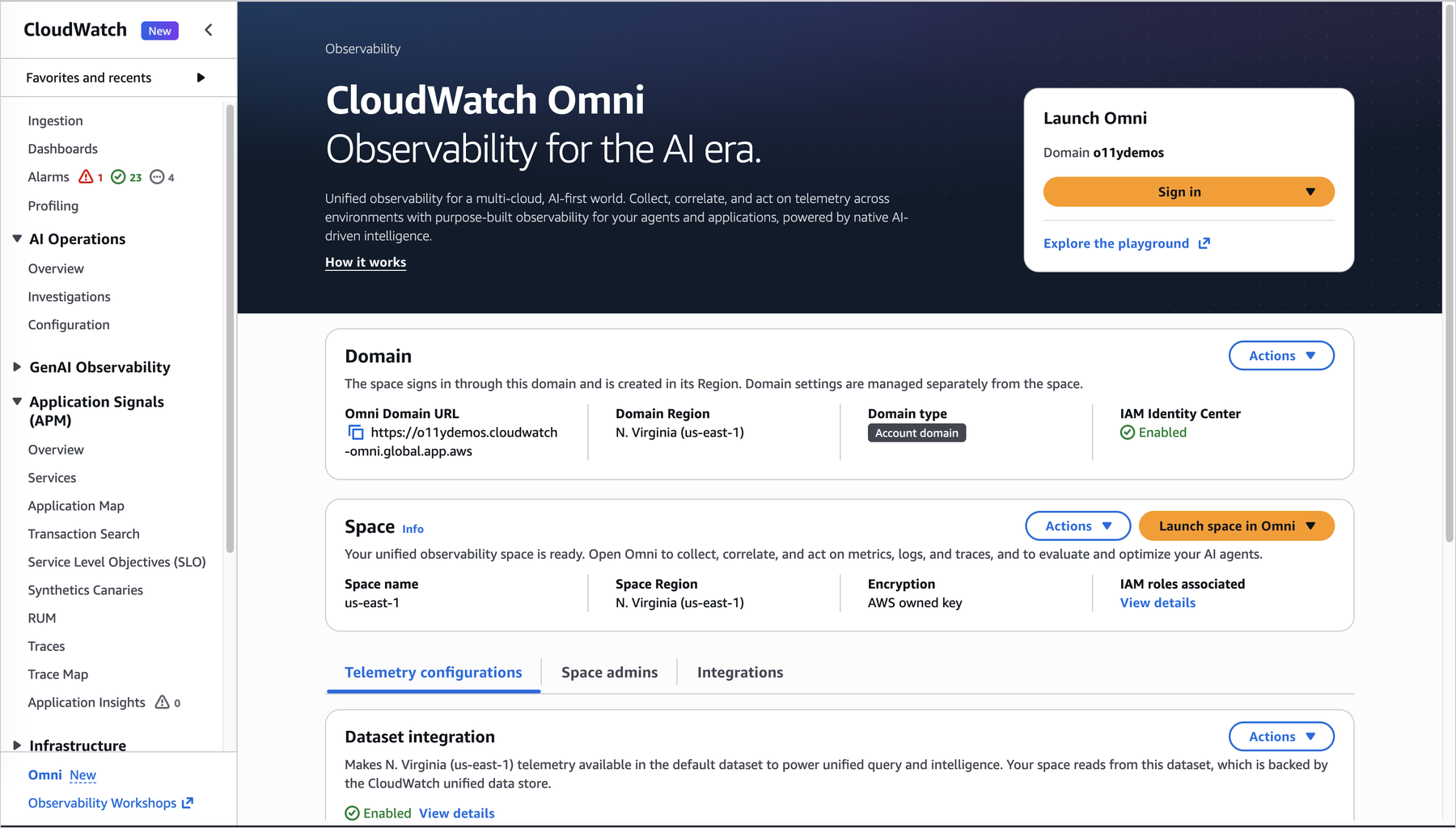
Modernizing SOAP applications using Amazon API Gateway and AWS Lambda

Post Syndicated from Daniel Abib original https://aws.amazon.com/blogs/compute/modernizing-soap-applications-using-amazon-api-gateway-and-aws-lambda/

This post demonstrates how you can modernize legacy SOAP applications using Amazon API Gateway and AWS Lambda to create bidirectional proxy architectures that enable integration between SOAP and REST systems without disrupting existing business operations.

Many organizations today face the challenge of maintaining critical business systems that were built decades ago. These legacy applications power essential business operations despite relying on outdated technologies and integration patterns. Although complete system replacement would be ideal, practical constraints such as budget limitations, resource availability, technical complexity, and missing documentation often make modernization efforts challenging.

This post first shows proxy architecture patterns to expose a legacy SOAP server over a REST API. It then shows how to integrate a legacy SOAP client with applications using a REST API.

While SOAP and REST APIs share HTTP as their foundation, SOAP has some limitations compared to REST, like limited HTTP methods (GET/POST only) and mandatory XML formatting. REST is more flexible with multiple HTTP methods and diverse payload formats (plain text, binary, HTML, JSON, XML).

Using API Gateway and Lambda to proxy SOAP service

Consider a legacy solution that only supports SOAP. The following diagram shows the architecture for a SOAP proxy server using API Gateway and Lambda.

Figure 1: SOAP Server Proxy for modernized architecture

Figure 1: SOAP Server Proxy for modernized architecture

The proxy exposes the APIs hosted on the SOAP Server (on the right side of the image) over a REST interface. A SOAP service expects the HTTP Content-Type header set to text/xml, and a XML format payload that follows the WSDL specification defined by the server.

In the proposed architecture, the Lambda function is the core transformation engine, handling the bidirectional conversion between JSON and XML formats. Lambda functions can be developed in multiple programming languages such as Python, Node.js, Java, C#, Go, Ruby, and PowerShell, allowing you to use your existing development expertise. The serverless nature of Lambda provides automatic scaling to handle traffic spikes without needing infrastructure management or capacity planning.

API Gateway acts as the intelligent front door, managing all incoming requests and routing them appropriately. It provides enterprise-grade features such as request throttling to protect backend systems from overload, comprehensive authentication and authorization mechanisms, API key management for partner access control, request and response validation, caching capabilities for improved performance, and detailed monitoring and logging. These built-in features remove the need for custom middleware development and provide immediate operational benefits. API Gateway can receive multiple payload format such as XML, JSON, binary data, and plain text. This makes it suitable for diverse integration scenarios.

Using API Gateway and Lambda to support legacy SOAP clients

The previous section focused on exposing SOAP services over REST APIs. Organizations also face the reverse challenge where legacy SOAP client applications must access REST services. The architecture for supporting legacy SOAP clients follows a similar pattern but with reversed data flow. In this case, the legacy SOAP client sends XML-formatted requests to what it believes is a SOAP server. However, behind the scenes API Gateway and Lambda work together to translate these requests into REST API calls.

Figure 2: Legacy SOAP client modernization architecture

Figure 2: Legacy SOAP client modernization architecture

The legacy SOAP client application sends XML SOAP messages to API Gateway. The Lambda function receives these SOAP requests, extracts the relevant data from the XML envelope, and transforms it into JSON format for the modern REST service.

The Lambda function wraps the JSON response from the REST services into the SOAP XML format that the legacy client expects. It recreates the appropriate XML structure, SOAP headers, and ensures that the response conforms to the WSDL specification that the client application was designed to consume.

Example scenario

Let’s suppose our legacy client application needs to send a SOAP request to convert an integer number to its word form. The SOAP envelop to convert the number 1519 to its long form “one thousand, five hundred and nine” looks like this:

<?xml version="1.0" encoding="utf-8"?>
<soap:Envelope xmlns:soap="http://schemas.xmlsoap.org/soap/envelope/">
    <soap:Body> \
        <ConvertNumberToWordsSoapIn>
            <NumberToWordsRequest>1519</NumberToWordsRequest>
        </ConvertNumberToWordsSoapIn>
    </soap:Body>
</soap:Envelope>

The REST conversion service expects a JSON payload the as follownig:

jsonObject = {
	"data" : 1519
}

The following code block shows a sample Lambda function implementation for this. This function converts the SOAP XML envelop to JSON, changes the http header to application/json, and converts response from REST service to SOAP format.

var parseString = require('xml2js').parseString;
const axios = require('axios');

exports.handler = async (event, context) => {
    var valueNumber;
    
    try {
        console.log("Parsing XML string");

        // Parsing the XML to obtain data needed for conversion (number to words)
        parseString(event.body, function (err, result) {
            if (!err) {
                valueNumber = result['soap:Envelope']['soap:Body'][0]
                              ['ConvertNumberToWordsSoapIn'][0]
                              ['NumberToWordsRequest'][0];
            } else { 
                console.log (err);
                throw (err);
            }
        });
        console.log("Creating JSON for calling the service");
        // Creating JSON to call service
        var jsonObject = {
            "data" : valueNumber
        }
        
        console.log("Calling Microservice (NumberToWords)");
        const headers = { 
            'Content-Type': 'Application/json'
        };
        
        console.log ("Parameter for NumberToWords URL:" + 
                    JSON.stringify(process.env.NumberToWordMicroservice));

        // Calling numberToWords REST Server
        var resultNumberToWords = await 
            axios.post(process.env.NumberToWordMicroservice, jsonObject, { headers });
        
        // Creating the response
        console.log("Creating response XML");

        var resp =  create_response (JSON.stringify(resultNumberToWords.data.message));
        console.log("Response in XML: "+ resp);
        
        // Returning the value in XML using text/xml content type
        let response = {'statusCode': 200, headers: {"content-type": "text/xml"}, 
                        'body': JSON.stringify(resp)}
        return response;
        
    } catch (err) {
        console.log ("Error: " + err);
        let response = {'statusCode': 500, 
                        headers: {"content-type": "text/xml"}, 'body': err}
        return response;
    }
};

// Function to create a SOAP XML envelope with the result value
function create_response(numberInWords) {
  return '<?xml version="1.0" encoding="utf-8"?> \
            <soap:Envelope xmlns:soap="http://schemas.xmlsoap.org/soap/envelope/">\
            <soap:Body>\
              <m:ConvertNumberToWordsResponse xmlns:m="http://www.dataaccess.com/webservicesserver/"> \
                  <m:ConvertNumberToWordsResponseResult>' + numberInWords + '</m:ConvertNumberToWordsResponseResult> \
              </m:ConvertNumberToWordsResponse> \
            </soap:Body>\
            </soap:Envelope>';
}

With this approach, you can maintain your existing SOAP client applications without modification, allowing them to consume modern REST services. You can preserve investments in legacy client applications while gradually modernizing the overall system. This architecture is particularly valuable in scenarios where multiple legacy SOAP clients need to access the same modern REST services. This is because a single proxy can serve multiple client applications simultaneously. The serverless nature of the architecture makes sure that it scales automatically based on the number of client requests, providing cost-effective operation regardless of usage patterns.

Alternative approach using API Gateway transformation capabilities

The Lambda-based approach provides maximum flexibility and control. API Gateway also offers built-in transformation capabilities that can handle certain SOAP modernization scenarios without the need for compute resources.

The native API Gateway transformation uses Apache Velocity Template Language mapping templates. It converts the payload directly at the gateway, offering a streamlined solution for specific modernization scenarios.

The VTL approach works by defining mapping templates that handle the conversion process between different payload formats. When modernizing SOAP services, these templates can intercept REST requests with JSON payloads, restructure the data into XML format compatible with your legacy SOAP endpoints, and reverse the process for responses returning to the client.

Figure 3: API Gateway with velocity template language transformation

Figure 3: API Gateway with velocity template language transformation

This gateway-native transformation strategy offers several operational advantages. You benefit from streamlined architecture because the transformation logic resides entirely within the API Gateway service. There are no other infrastructure components to manage or monitor, and the solution avoids the complexity of coordinating between multiple AWS services. Cost efficiency is another key benefit, as there are no compute charges beyond the standard API Gateway pricing.

Consider the previous example of converting a number to its word format. The VTL transformation in API Gateway will look like this:

## Parse the SOAP envelope and extract the number value
#set(\$xmlDoc = \$input.path('\$'))
#set(\$numberToWords = \$xmlDoc.Envelope.Body.ConvertNumberToWordsSoapIn.NumberToWordsRequest)

## Convert to integer if it's a string
#if(\$numberToWords.toString().matches("^\d+\$"))
  #set(\$dataValue = \$numberToWords.toInteger())
#else
  #set(\$dataValue = \$numberToWords)
#end

{
  "data": \$dataValue
}

You should consider VTL transformations when your SOAP services have predictable, stable schemas with relatively direct XML structures. This approach works particularly well for legacy systems that rarely undergo changes and have clear request-response patterns. For more dynamic environments or complex transformation requirements, the Lambda-based solution provides superior flexibility and maintainability.

Security considerations

An important consideration when working with legacy SOAP services is understanding their authentication mechanisms. SOAP protocols often implement authentication through security standards, where authentication credentials and security tokens are embedded directly within the SOAP envelope headers. This includes username tokens, digital signatures, and encryption elements that are part of the XML structure.

When SOAP envelopes contain unencrypted authentication information in the headers, the proxy architecture typically functions without more modifications. This is because the Lambda function can pass through these authentication elements transparently to the backend SOAP service. However, due to the nature of SOAP authentication being tightly integrated with the XML envelope structure, certain scenarios may need custom handling within the Lambda function.

For example, if the SOAP service uses timestamp-based authentication tokens, session management, or needs specific security header modifications, the Lambda function may need customization to properly handle, validate, or refresh these authentication elements during the JSON-to-XML transformation process. Organizations should carefully analyze their SOAP service authentication requirements to determine if more Lambda logic is needed to maintain security compliance.

Moreover, make sure that any SOAP authentication credentials processed by the Lambda function are handled securely and never logged in plain text.

Conclusion

In this post, you learned how cloud-native services can bridge the gap between legacy systems and modern application architectures, allowing you to use your existing investments while adopting contemporary development practices and technologies.

Amazon API Gateway and AWS Lambda enable organizations to create REST services that proxy legacy SOAP servers, allowing modern applications to consume legacy services through JSON payloads while preserving existing SOAP infrastructure. This serverless solution provides cost-effectiveness, automatic scaling, and reduced operational overhead while facilitating company modernization through scalable APIs without abandoning legacy software investments.

This modernization strategy allows you to gradually transition from legacy SOAP services to modern REST APIs without disrupting existing business operations. As your modernization journey progresses, you can extend this pattern to support more SOAP services or implement more sophisticated transformation logic based on your specific business requirements.

For more serverless learning resources, visit Serverless Land.