Amazon S3 Tables, a capability of Amazon Simple Storage Service (Amazon S3), deliver a cloud object store with built-in Apache Iceberg support and streamline storing tabular data at scale. When you integrate them with dbt and AWS Glue, you can run SQL-based data transformations with the reliability and performance of a modern lakehouse, bringing software engineering best practices to the data space.
This post demonstrates how to configure and implement dbt transformations using Amazon S3 Tables with the dbt-glue adapter. Starting with version 1.12.4, the dbt-glue adapter adds incremental merge support for S3 Tables, which the patterns in this post build on. We cover the specific configuration requirements for the dbt-glue adapter and practical implementation patterns built on S3 Tables incremental models: the merge strategy to keep the latest state per record and the append strategy to build an audit-friendly change history.
Example scenario
In this walkthrough, we simulate an ecommerce system that tracks customer profiles and their orders. We first run the pipeline against an initial dataset, then simulate an update to the upstream source data and run it again to demonstrate incremental updates.
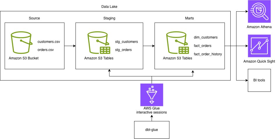
Our example scenario follows a data pipeline architecture that uses S3 Tables throughout. Raw ecommerce data (customers.csv and orders.csv) lands in a regular S3 bucket as comma-separated values (CSV). dbt then transforms it through two layers of S3 Tables. A staging layer cleanses and standardizes each source, and a mart layer produces analytics-ready dimension and fact tables. You can query the resulting mart data from a variety of analytics and business intelligence (BI) tools such as Amazon Athena and Amazon Quick Sight. In this post, we query it from Athena.
The mart layer demonstrates two incremental strategies side by side: the fact_orders model uses merge to keep the latest state per order, while fact_order_history uses append to accumulate a full change history.
The data pipeline flow looks like the following chart:
Source Data (Regular S3 - CSV)
    └─ customers.csv, orders.csv
    ↓
Staging Models (S3 Tables)
    ├─ stg_customers
    └─ stg_orders
    ↓
Mart Models (S3 Tables)
    ├─ dim_customers
    ├─ fact_orders                (incremental with merge --- latest state per order)
    └─ fact_order_history         (incremental with append --- change history)
    ↓
Consumption Layer (Athena, Quick Sight, BI tools)
The following diagram shows the architecture behind this pipeline: dbt-glue submits each model as a Spark SQL statement to an AWS Glue interactive session, which reads from the raw S3 bucket and writes the staging and mart tables as S3 Tables within the same data lake.
Figure 1: Architecture of the dbt transformation pipeline on Amazon S3 Tables with AWS Glue
Prerequisites
Before you begin, make sure that you have the following prerequisites:
In this section, you set up the AWS infrastructure that dbt-glue needs: an S3 table bucket and namespace to hold your dbt models, and an AWS Glue database for your source data.
First, set your environment variables. Replace YOUR_ACCOUNT_ID, YOUR-REGULAR-BUCKET, and YOUR_Glue_Role_ARN with your data:
Note that the S3 Tables namespace is where the S3 Tables corresponding to your dbt models will be created. This is different from regular S3 buckets. Because the “Integration with AWS analytics services” option for S3 Tables is enabled, creating the namespace automatically creates a corresponding AWS Glue database. Verify that it exists in the next step:
In this section, you create sample ecommerce data to transform with dbt: two CSV files (customers and orders), upload them to a general purpose S3 bucket, and register them as AWS Glue tables that your dbt models can read from.
Note: All sample data in this post is synthetic. It was generated to mimic realistic patterns for demonstration purposes only and doesn’t represent any real individuals or transactions.
Complete following steps to create a sample dataset:
Create a directory for sample data and save the following two CSV files: customers.csv:
Create the bucket for source data if it doesn’t exist, and upload the CSV files to the S3 bucket. Replace YOUR-SOURCE-DATA-BUCKET with your bucket name.
The dbt CLI is a command-line interface for running dbt projects. It’s free to use and available as an open source project. Before installing dbt-core, make sure your Python version is 3.10, 3.11, or 3.12.
Install dbt and the dbt CLI with the following code:
Install the dbt-glue adapter with the following code:
$ pip3 install --no-cache-dir dbt-glue
Note that you need to install dbt-glue 1.12.4 or higher, which adds support for incremental append and merge models on S3 Tables.
Create a dbt project
In this section, you create a new dbt project using dbt init, which generates the standard directory structure (such as models, macros, and tests) that you will populate with the S3 Tables models in the next sections.
Run the dbt init command to create and initialize a new empty dbt project.
$ dbt init
For a project name, enter dbt_glue_s3_tables.
For a database, choose [1] glue.
Please ignore dbt_project.yml file [ERROR not found] message as we are going to create it in the next step.
Configure dbt profile
The dbt profile configuration is critical for S3 Tables integration. In this section, you create a dbt profile that connects to AWS Glue Interactive Sessions and configures Spark to read and write S3 Tables through the Iceberg catalog, then validate the connection with dbt debug.
Create ~/.dbt/profiles.yml with the following structure:
Run the following command to validate the configurations:
cd dbt_glue_s3_tables
dbt debug --profiles-dir ~/.dbt/
Expected output is Connection test: [OK connection ok].
Configure dbt project
The dbt_project.yml configuration determines which models use S3 Tables. Create or update dbt_glue_s3_tables/dbt_project.yml with the following structure:
name: 'dbt_glue_s3_tables'
version: '1.0.0'
config-version: 2
profile: 'dbt_glue_s3_tables'
model-paths: ["models"]
test-paths: ["tests"]
macro-paths: ["macros"]
models:
  dbt_glue_s3_tables:
    # S3 Tables for staging
    staging:
      +materialized: table
      +file_format: 's3tables'  # S3 Tables for staging
      +table_properties:
        'format': 'iceberg'
        'write.format.default': 'parquet'
        'write.parquet.compression-codec': 'snappy'

    # S3 Tables for marts
    marts:
      +materialized: table
      +file_format: 's3tables'  # S3 Tables for marts
      +table_properties:
        'format': 'iceberg'
        'write.format.default': 'parquet'
        'write.parquet.compression-codec': 'snappy'
Create dbt models
In this section, you build out the full model layer: a sources.yml that registers your raw AWS Glue tables, two staging models that clean and prepare the customer and order data, and three mart models that turn those staged data into a dimension table and two fact tables, one using incremental merge and one using incremental append.
First, create sources.yml defines your raw data tables:
Delete the example folder under dbt_glue_s3_tables/models. This is an example folder created by default and unnecessary now.
Define source tables in models/sources.yml with the following structure:
This sources.yml defines your raw data tables, so you can reference them with the {{ source() }} function in your models. With this file, you can also define data tests like unique, not_null, and referential integrity checks in one central place.
Second, create the staging and mart models. Staging models are where you unpack and transform raw data. Mart models are what downstream consumers actually query.
Create models/staging/stg_customers.sql:
-- Staging model as S3 Tables with incremental merge
{{ config(
    materialized='incremental',
    incremental_strategy='merge',
    unique_key='customer_id',
    on_schema_change='sync_all_columns',
    file_format='s3tables'
) }}

SELECT
    customer_id,
    LOWER(TRIM(email)) AS email,
    first_name,
    last_name,
    CAST(registration_date AS DATE) AS registration_date,
    customer_segment
FROM spark_catalog.{{ source('raw_ecommerce', 'customers') }}
WHERE customer_id IS NOT NULL
stg_customers.sql reads from the raw customers source, applies light cleansing (email normalization, date casting, null filtering), and writes to S3 Tables using an incremental merge on customer_id to update existing records rather than duplicating them.
Create models/staging/stg_orders.sql:
-- Staging model as S3 Tables with incremental merge
{{ config(
    materialized='incremental',
    incremental_strategy='merge',
    unique_key='order_id',
    on_schema_change='sync_all_columns',
    file_format='s3tables'
) }}

SELECT
    order_id,
    customer_id,
    CAST(order_date AS DATE) AS order_date,
    CASE
        WHEN LOWER(TRIM(order_status)) = 'completed'  THEN 'completed'
        WHEN LOWER(TRIM(order_status)) = 'shipped'    THEN 'shipped'
        WHEN LOWER(TRIM(order_status)) = 'processing' THEN 'processing'
        WHEN LOWER(TRIM(order_status)) = 'cancelled'  THEN 'cancelled'
        ELSE 'unknown'
    END AS status,
    CAST(order_amount AS DECIMAL(10,2)) AS total_amount,
    EXTRACT(YEAR  FROM CAST(order_date AS DATE)) AS order_year,
    EXTRACT(MONTH FROM CAST(order_date AS DATE)) AS order_month,
    CAST(updated_at AS TIMESTAMP) AS updated_at
FROM spark_catalog.{{ source('raw_ecommerce', 'orders') }}
WHERE order_id IS NOT NULL
stg_orders.sql reads from the raw orders source, normalizes status to a fixed set of values (defaulting to unknown for anything unexpected), casts order_date, total_amount, and updated_at to their proper types, and derives order_year and order_month for downstream partitioning.
Create models/marts/dimensions/dim_customers.sql:
-- Dimension table using S3 Tables
{{ config(
    materialized='table',
    file_format='s3tables',
    partition_by=['registration_year'],
    table_properties={
        'format': 'iceberg',
        'write.format.default': 'parquet'
    }
) }}

SELECT
    customer_id,
    email,
    first_name,
    last_name,
    registration_date,
    YEAR(registration_date) as registration_year,
    customer_segment,
    CASE
        WHEN customer_segment = 'Premium' THEN 1
        WHEN customer_segment = 'Regular' THEN 2
        ELSE 3
    END as segment_priority,
    CURRENT_TIMESTAMP() as dbt_updated_at
FROM {{ ref('stg_customers') }}
Create models/marts/facts/fact_orders.sql:
-- Fact table using S3 Tables with incremental merge
{{ config(
    materialized='incremental',
    file_format='s3tables',
    incremental_strategy='merge',
    unique_key='order_id',
    partition_by=['order_year', 'order_month'],
    table_properties={
        'format': 'iceberg',
        'write.format.default': 'parquet'
    }
) }}

SELECT
    o.order_id,
    o.customer_id,
    o.order_date,
    YEAR(o.order_date)  AS order_year,
    MONTH(o.order_date) AS order_month,
    o.status,
    o.total_amount,
    c.customer_segment,
    c.segment_priority,
    CURRENT_TIMESTAMP() AS dbt_updated_at
FROM {{ ref('stg_orders') }} o
LEFT JOIN {{ ref('dim_customers') }} c
  ON o.customer_id = c.customer_id
Create models/marts/facts/fact_order_history.sql:
-- Fact table using S3 Tables with incremental append
{{ config(
    materialized='incremental',
    file_format='s3tables',
    incremental_strategy='append',
    partition_by=['event_year', 'event_month'],
    table_properties={
        'format': 'iceberg',
        'write.format.default': 'parquet'
    }
) }}

SELECT
    order_id,
    customer_id,
    status,
    order_date,
    total_amount,
    updated_at,
    CURRENT_TIMESTAMP() AS recorded_at,
    YEAR(updated_at)    AS event_year,
    MONTH(updated_at)   AS event_month
FROM {{ ref('stg_orders') }}

{% if is_incremental() %}
    WHERE updated_at > (SELECT MAX(updated_at) FROM {{ this }})
{% endif %}
Run the dbt project
Now it’s time to run the dbt project. Complete following steps:
To run the project dbt, you should be in the project folder:
cd dbt_glue_s3_tables
Run the dbt command:
dbt run --profiles-dir ~/.dbt/ --full-refresh
This command starts an AWS Glue interactive session, compiles the dbt models, and materializes all five tables (stg_customers, stg_orders, dim_customers, fact_orders, and fact_order_history) in your S3 Tables namespace. The --full-refresh flag rebuilds the incremental models from scratch, so it’s the right choice for the first run.
Query using Amazon Athena
Before testing the incremental merge and append behavior in the next section, confirm what the initial --full-refresh run loaded into the mart tables. Query the target tables.
In the Athena console, choose the data source and database that correspond to your S3 Tables catalog:
Run the following query to view the data loaded into the fact_orders table:
SELECT * FROM dbt_glue_s3_tables.fact_orders ORDER BY order_id;
The result returns the five order records:
#    order_id    customer_id    order_date    order_year    order_month    status    total_amount    customer_segment    segment_priority    dbt_updated_at
1    1001    1    2024-06-01    2024    6    completed    150.00    Premium    1    2026-10-16 09:41:46.590373 UTC
2    1002    2    2024-06-02    2024    6    completed    75.50    Standard    3    2026-10-16 09:41:46.590373 UTC
3    1003    1    2024-06-03    2024    6    completed    200.00    Premium    1    2026-10-16 09:41:46.590373 UTC
4    1004    3    2024-06-04    2024    6    unknown    125.75    Premium    1    2026-10-16 09:41:46.590373 UTC
5    1005    4    2024-06-05    2024    6    completed    89.99    Standard    3    2026-10-16 09:41:46.590373 UTC
Run the following query to view the data loaded into the fact_order_history table:
SELECT * FROM dbt_glue_s3_tables.fact_order_history ORDER BY updated_at;
The result returns the five order history records.
#    order_id    customer_id    status    order_date    total_amount    updated_at    recorded_at    event_year    event_month
1    1001    1    completed    2024-06-01    150.00    2024-06-01 10:00:00.000000 UTC    2026-10-16 09:41:22.801835 UTC    2024    6
2    1002    2    completed    2024-06-02    75.50    2024-06-02 10:00:00.000000 UTC    2026-10-16 09:41:22.801835 UTC    2024    6
3    1003    1    completed    2024-06-03    200.00    2024-06-03 10:00:00.000000 UTC    2026-10-16 09:41:22.801835 UTC    2024    6
4    1004    3    unknown    2024-06-04    125.75    2024-06-04 10:00:00.000000 UTC    2026-10-16 09:41:22.801835 UTC    2024    6
5    1005    4    completed    2024-06-05    89.99    2024-06-05 10:00:00.000000 UTC    2026-10-16 09:41:22.801835 UTC    2024    6
Incremental merge and append on Iceberg table
After the initial --full-refresh run succeeds, verify that the merge and append incremental strategies behave as expected when the source data changes. This demonstrates the row-level update capability that Iceberg on S3 Tables provides.
Update the sample source data
To simulate a real-world scenario where upstream source data changes over time (for example, a customer updating their profile, or new customers signing up), modify customers.csv to include both an update to an existing record and a new record.
order_id=1004: status updated from pending to completed with a later updated_at (to test the merge UPDATE).
order_id=1006: new record added with a later updated_at, associated with the new customer customer_id=6 (to test both the merge INSERT in fact_orders and the append in fact_order_history).
By running without --full-refresh, dbt runs its normal incremental logic instead of rebuilding the tables from scratch. In the staging layer, stg_customers and stg_orders apply the changes with a MERGE INTO statement that updates customer_id=1 and order_id=1004 in place and inserts customer_id=6 and order_id=1006. Downstream, fact_orders (merge) reflects the 1004 update and the 1006 insert as the latest state, while fact_order_history (append) records both 1004 and 1006 as new history rows.
Verify the results in Amazon Athena
After the re-run completes, use Athena to confirm that the merge and append strategies behaved as expected.
Run the following query to view the updated data in the fact_orders table:
SELECT * FROM dbt_glue_s3_tables.fact_orders ORDER BY order_id;
fact_orders returns 6 rows (one per order), with 1004 now completed and 1006 added.
#    order_id    customer_id    order_date    order_year    order_month    status    total_amount    customer_segment    segment_priority    dbt_updated_at
1    1001    1    2024-06-01    2024    6    completed    150.00    Premium    1    2026-10-16 10:06:55.944983 UTC
2    1002    2    2024-06-02    2024    6    completed    75.50    Standard    3    2026-10-16 10:06:55.944983 UTC
3    1003    1    2024-06-03    2024    6    completed    200.00    Premium    1    2026-10-16 10:06:55.944983 UTC
4    1004    3    2024-06-04    2024    6    completed    125.75    Premium    1    2026-10-16 10:06:55.944983 UTC
5    1005    4    2024-06-05    2024    6    completed    89.99    Standard    3    2026-10-16 10:06:55.944983 UTC
6    1006    6    2024-07-02    2024    7    completed    45.00    Premium    1    2026-10-16 10:06:55.944983 UTC
Run the following query to view the updated data in the fact_order_history table:
SELECT * FROM dbt_glue_s3_tables.fact_order_history ORDER BY updated_at;
fact_order_history grows from 5 rows to 7 rows on the second run (the 2 rows whose updated_at advanced: 1004 and 1006). Order 1004 now has two history rows: the original unknown status and the new completed status.
#    order_id    customer_id    status    order_date    total_amount    updated_at    recorded_at    event_year    event_month
1    1001    1    completed    2024-06-01    150.00    2024-06-01 10:00:00.000000 UTC    2026-10-16 09:41:22.801835 UTC    2024    6
2    1002    2    completed    2024-06-02    75.50    2024-06-02 10:00:00.000000 UTC    2026-10-16 09:41:22.801835 UTC    2024    6
3    1003    1    completed    2024-06-03    200.00    2024-06-03 10:00:00.000000 UTC    2026-10-16 09:41:22.801835 UTC    2024    6
4    1004    3    unknown    2024-06-04    125.75    2024-06-04 10:00:00.000000 UTC    2026-10-16 09:41:22.801835 UTC    2024    6
5    1005    4    completed    2024-06-05    89.99    2024-06-05 10:00:00.000000 UTC    2026-10-16 09:41:22.801835 UTC    2024    6
6    1004    3    completed    2024-06-04    125.75    2024-06-11 09:30:00.000000 UTC    2026-10-16 10:06:35.291993 UTC    2024    6
7    1006    6    completed    2024-07-02    45.00    2024-07-02 10:00:00.000000 UTC    2026-10-16 10:06:35.291993 UTC    2024    7
Clean up
To avoid ongoing charges, clean up the resources you created during this walkthrough. Complete these steps in the specified order to facilitate proper resource deletion.
Drop the tables dbt created in the S3 Tables namespace.
Delete the data this walkthrough wrote to your S3 bucket: the dbt warehouse data under s3://<YOUR-REGULAR-BUCKET>/glue/data/ and the sample CSV files under s3://<YOUR-REGULAR-BUCKET>/raw/. Leave the bucket itself in place if you use it for other workloads.
(Optional) Remove the local dbt project directory (dbt_glue_s3_tables) and the sample customers.csv / orders.csv files.
Conclusion
In this post, we showed how to build an end-to-end dbt transformation pipeline on Amazon S3 Tables with AWS Glue 6.0, using a staging and mart architecture. At the core of this pipeline are incremental models on S3 Tables, which let us transform and maintain data incrementally with SQL. We demonstrated two incremental strategies working together: the merge strategy to keep the latest state per order in fact_orders, and the append strategy to build an audit-friendly change history in fact_order_history.
S3 Tables support in the dbt-glue adapter is currently experimental (as of version 1.12.4) and will continue to evolve in upcoming releases. As with any experimental feature, we recommend thoroughly testing it in your own environment before use.
The BPF verifier has historically worked by tracing every possible path of
execution through a program, checking, at each instruction, that various safety
properties hold. This works, but it can result in an exponential increase in the
number of states that need checking in programs with complicated control-flow.
Alexei Starovoitov, one of the kernel’s core BPF maintainers, has shared
a patch set that substantially reworks how the verifier tracks states, in
order to reduce the size of that exponential explosion.
The PostgreSQL Global Development Group has announced
the release of PostgreSQL 19. Notable features in this release include the
introduction of the REPACK (CONCURRENTLY) command to optimize tables
without disruption to ongoing operations, better control over plan stability and
query performance with the new pg_plan_advice extension, and a number
of performance improvements.
In September, LWN covered the
removal of several features initially slated for this release. See the release notes for
a full list of new features and changes.
When an MDR provider contains a compromised endpoint, your team needs to know whether the weakness that enabled the attack exists elsewhere and who is responsible for addressing it. Without that follow-through, the immediate incident may be resolved while another attacker still has a way in.
Preemptive managed detection and response (MDR) is Rapid7’s approach to connecting exposure context, threat intelligence, AI-assisted investigation, and human expertise. It supports proactive cybersecurity by helping teams prioritize weaknesses before exploitation, investigate threats with a clearer understanding of risk, and use their findings to strengthen defenses.
How does preemptive MDR differ from traditional MDR?
Managed detection and response provides security specialists who monitor, investigate, and respond to threats around the clock. Many services also include proactive threat hunting and recommendations to improve security.
Preemptive MDR connects that work more directly to what makes an organization vulnerable. When analysts investigate suspicious activity on a server, knowing that it is internet-facing, supports a critical application, and has a vulnerability under active exploitation helps them assess urgency and determine where to look next.
In Rapid7’s model, exposure findings inform investigation and remediation priorities, while investigations reveal weaknesses that need attention. Security leaders gain a clearer connection between the threats their provider handles and the conditions their organization needs to address.
Within a broader preemptive cybersecurity strategy, MDR connects exposure information with the people investigating and responding to threats. The aim is to reduce opportunities for compromise and intervene before an attack causes harm, while retaining the expertise to contain and recover from incidents.
How exposure context and proactive threat hunting inform MDR
By combining information about assets, vulnerabilities, business criticality, and attacker behavior, preemptive MDR helps teams decide which weaknesses require action first. Exposure context also informs targeted hunting and the investigation of suspicious activity.
Consider a hypothetical organization running an internet-facing application affected by a newly disclosed vulnerability. The security team needs to establish whether the vulnerable software is present, what the application supports, and whether attackers are exploiting the weakness.
Those findings can guide remediation priorities and targeted hunting for signs of compromise. If suspicious activity appears, analysts investigate it with an understanding of the affected system and the potential route an attacker could take through the environment.
Depending on the evidence, the response may involve containing a system, examining related accounts, or expanding the investigation to other assets. The organization’s remediation teams also need clear recommendations about the underlying exposure.
What the investigation reveals then feeds back into detection rules, hunting priorities, and response procedures. This gives leaders a way to track an identified risk through investigation, action, and outstanding work, with clearer ownership at each stage.
What role does AI play in preemptive MDR?
Before analysts can assess a potential threat, they often need to retrieve logs, examine user activity, and connect evidence across several systems. AI can accelerate this work by gathering and correlating information for review.
Agentic investigation capabilities can perform elements of that process in parallel, test possible explanations, and organize findings. Their usefulness depends on the available data: missing identity activity or asset information can leave gaps in the account of what happened.
Rapid7’s approach keeps human expertise central to validation and response decisions. Analysts assess the evidence alongside the organization’s priorities and the consequences of an action, including whether isolating a system could interrupt a critical service.
What to look for in a preemptive MDR provider
When evaluating a service described as preemptive, ask the provider to show how exposure information changes its work. A redacted investigation should make clear what analysts knew about the affected asset, how that influenced their reasoning, and which actions followed.If an investigation identified a weakness, was it assigned to an owner and addressed? Did the findings change detection coverage or future priorities? Where AI contributed, the provider should explain its role and the oversight applied.
Incident response remains part of the requirement. Rapid7 MDR includes unlimited incident response alongside exposure-informed defense and AI-assisted investigation, supporting containment, detailed analysis, and threat eradication.
Agree on responsibilities before that support is needed. Establish which actions the provider can take, when customer approval is required, and who owns remediation. Those arrangements determine how findings become action, particularly when taking a system offline carries business consequences.
Once the service is operating, review progress through specific cases: exposures addressed before exploitation, threats contained, and weaknesses closed after investigation. Ask to see the evidence behind those outcomes and any work still outstanding, so your team can judge where risk has changed and where further attention is needed.
Explore Rapid7 MDR to see how exposure-informed defense, AI-assisted investigation, and expert response work together.
For a threat actor, the perfect malware is one they don’t have to write, and already does all they need. One example of this is shown by the China-aligned APT known as Webworm, which has been known to deploy the open-source SoftEther VPN into the networks of compromised governmental organizations to maintain low-profile, long-term access.
After this was publicly documented and defenders could keep an eye out for this tactic, the actor presumably started thinking of ways to make their covert access stealthier. In this post, we share our analysis of what we believe to be a so-far unknown custom SoftEther-based tool, which implements various tricks to hide itself from security tools, and which we attribute to Webworm with moderate confidence. We additionally provide guidance and tooling for detecting its presence on a system and extracting the configuration(s) associated with it.
Technical analysis
To illustrate how the tool works, we will use the only public sample of this tool we are aware of, which can be found in our IoCs list (90e7…).
The sample is a Windows PE32+ file targeting the x64 architecture. Based on cleartext strings and constants in the binary, we identified it as a (modified) build of the SoftEther VPN Bridge executable, specifically version 4.44, build 9807. Similarly, the PDB path included in the executable reads C:\Users\Administrator\Desktop\SoftEtherVPN_Stable\SoftEtherVPN_Stable\SoftEtherVPN_Stable\src\DebugFiles\pdb\x64_Release\vpnbridge.pdb. As such, the tool doesn’t hide its identity from reverse engineers, only external interactions.
The first and most trivial change the threat actor implements is in the PE metadata. Here we learn that the OriginalFileName of this binary is netcapa.exe, and it brands itself as “Network Monitor Software” published by a company named “Network Systems Solutions Inc.“. The only field unchanged against the stock SoftEther executable (vpnbridge_x64.exe) is the Version, which reads 4, 44, 0, 9807.
Next, we wanted to identify any functionality added or modified by the threat actor. The SoftEther bridge alone is a powerful tool to maintain remote access to a compromised network, but we wanted to know if perhaps there was a backdoor to give the threat actor direct command execution on the infected host. For that reason we checked out the corresponding tag in the public “SoftEtherVPN_Stable” repository on GitHub and compared it to the decompiled sample.
Internal rebranding
The rebranding apparent in the exposed metadata extends into internal strings used in debug banners, service names, registry keys, the contents of the server’s HTTP 401 error page, or firewall rule names, where occurrences of “SoftEther VPN” are replaced by “NtMonitor VPN”.
However, the renaming is inconsistent; for example, the service name used by the entry point is still SEVPNBRIDGE, and many registry key paths still reference the “SoftEther Project”.
Network stealth
Stock SoftEther VPN Mayaqua/Network.h defines HTTP endpoints used by the protocol:
A client initiating a connection to a SoftEther VPN server will send a handshake request to HTTP_VPN_TARGET2 along with a “watermark”, i.e. a byte pattern proving that the client is speaking the correct VPN protocol. Otherwise, the server answers with a decoy HTTP response.
NtMonitor changes the upstream GIF watermark with a custom byte pattern (a truncated PNG file showing the Windows logo), so that stock SoftEther clients and servers cannot handshake with this build, and NtMonitor’s own peers cannot be fingerprinted with the well-known stock GIF watermark.
Embedded resource archive
As the threat actor probably realizes, a SoftEther resource archive named hamcore.se2, which sits next to the executables in the installation directory and is required to be present at runtime, provides a straightforward detection opportunity for unauthorized installations. We think that, for this exact reason, the actor chose to reduce the contents of this archive to a bare minimum, package the archive inside the bridge executable itself (as a PE resource), and implement a custom resource directory walk to load the archive at runtime. As a side effect, this increases the binary’s size by about 1.5 MB compared to the official build.
Encrypted configuration
Another weak point (for the attacker) in stock SoftEther is that its configuration is stored on disk in plain text in a well-recognizable format. The actor changes its name from vpn_bridge.config to setting.conf and modifies the configuration loader to handle custom-encrypted files that start with the magic bytes RCEN in ASCII. The rest of the encrypted file has a simple format and includes the encryption key. A Python script to decrypt such files with the actor’s custom RC4-like cipher is available on the Rapid7 Intelligence GitHub repository.
Attribution and interpretation of findings
Beyond the changes described above, we did not identify any additional malware functionality. Clearly, the threat actor prioritizes stealth above raw capability. It seems like they methodically analyzed SoftEther’s detection surface and implemented counter-measures to all of the easy ways a detection engineer may target it. At the time of our analysis, only one anti-virus vendor detected the sample on VirusTotal, although it has been public since January.
This aligns well with the TTPs previously reported for Webworm by ESET, and such attribution is further supported by indicators in decrypted configurations Rapid7 Intelligence has access to. In all of the cases, the VPN is configured to bridge (“cascade”) a remote network into the local one; furthermore, in cases that were not likely deliberate tests, the remote IP address was located inside AS 20473 belonging to The Constant Company, LLC, which (also including its subsidiary, Vultr) has been associated with Webworm on many occasions in the past.
Considering this attribution, we can put together some important takeaways: Quite likely, we are looking at a new evolution in the tooling used by Webworm, a China-aligned APT whose activity is known to focus on governmental organizations, especially in Europe. Earlier this year, ESET already noted this group to shift away from custom malware to dual-use tools such as SoftEther VPN, but now we are observing a sort of hybrid of the two — stock SoftEther software that is not trojanized, but rebuilt from source in a way that erases much of its detection fingerprint.
Detection guidance
To detect this particular variant of Webworm’s tooling, we provide a list of IoCs and a YARA ruleset on our public GitHub repository. If you have the ability to inspect TLS traffic in your organization, one of the most reliable detections you can deploy right now is to look for POST requests to /update/picture.cgi with Content-Type: image/jpeg and a request body starting with and 89 50 4e 47 0d 0a 1a 0a 00 00 00 0d 49 48 44 52 (initial bytes of the custom PNG watermark).
Although the samples we have seen all use the same NtMonitor branding internally (despite the PE metadata differing across samples), this is the easiest change for the threat actor to implement next. Similarly, the HTTP endpoints and watermark can be swapped out trivially. As such, we recommend defenders in the government sector to familiarize themselves with intrinsic SoftEther VPN behavior in order to stay one step ahead of when the threat actor decides to update the tool next.
MITRE ATT&CK techniques
Technique ID
Technique Name
Comment
T1587.001
Develop Capabilities: Malware
The actor is maintaining their own fork of SoftEther VPN used for malicious purposes.
T1027.013
Obfuscated Files or Information: Encrypted/Encoded File
Configuration files are encrypted with a custom cipher.
T1140
Deobfuscate/Decode Files or Information
Encrypted configuration files are decrypted at startup by the modified loader.
T1036.005
Masquerading: Match Legitimate Resource Name or Location
PE metadata is purposefully changed to masquerade as a generic system service.
T1027.005
Obfuscated Files or Information: Indicator Removal from Tools
Known SoftEther artifacts are systematically removed from the binary.
T1686.003
Disable or Modify System Firewall: Windows Host Firewall
Using stock SoftEther functionality, the malware adds rules to the system firewall.
T1599
Network Boundary Bridging
The VPN bridge binds together the infected host’s local area network with the attacker’s.
T1071
Application Layer Protocol
C2 communication uses HTTP(S) and SoftEther’s application protocol.
T1090.001
Proxy: Internal Proxy
The infected host serves as an internal proxy mediating C2 access to other hosts on the network.
Version 8.6.0 of
PHP has been released. Notable changes in this release include a polling API, a
new clamp() function, a SortDirection enum, and a \Time\Duration class. See “What’s new in 8.6”
for more on new features, and the changelog for a full list
of changes.
The PHP Project has announced the release of PHP 8.5.13, 8.4.28, 8.3.37, and 8.2.36. Each contains a
number of security and bug fixes, including several fixes for critical
vulnerabilities that could allow remote-code execution. According to the
project’s pre-release
announcement on November 18, all of the vulnerabilities of critical
severity “require either non-default configuration or uncommon
setups“. See the release notes for details; Linux vendors and projects
should be releasing updated packages soon.
Visitors to government election websites surged 363% on November 3, the date of the 2026 midterm elections in the United States. Across Cloudflare's election protection programs, we also detected a significant shift in the types and timing of cyberattacks throughout 2026.
Unlike what we saw in other recent elections, attackers focused on gaining access to internal systems and data, rather than knocking websites offline. Government election websites faced website vulnerability attempts 180 times more often than denial-of-service (DDoS) attacks, and at roughly ten times the rate of Cloudflare's broader customer base. We also found evidence of at least one attempt to exploit a recently disclosed critical PHP vulnerability on a state government voting website in the Western United States.
These attacks peaked in late October, several weeks before the election. Vulnerability exploit attempts climbed steadily throughout 2026: from 200,000 per day in January, to 2 million per day in October. However, on Election Day in the U.S., Cloudflare detected no escalation in attack volume and zero major DDoS incidents across protected election sites, marking a sharp contrast to other recent elections, such as in Moldova last year.
Our data regarding cyberattacks on election institutions came from organizations participating in Cloudflare's free cybersecurity programs: the Athenian Project, Cloudflare for Campaigns, and Project Galileo. Together, these initiatives helped protect more than 1,400 election-related websites during the 2026 U.S. midterm elections, including those belonging to state and local governments, candidates, political parties, voting-rights advocates, journalists, and civil society groups.
Cloudflare launched its first election protection program in 2016 after widespread reports of cyberattacks targeting the U.S. elections. A decade later, it is remarkable to see how far governments and campaigns have come in securing their digital infrastructure. We are proud to help protect democratic institutions and are encouraged that cyberattacks were once again not a disruptive factor in 2026.
In this post, we examine traffic and attacks observed against those organizations on Election Day, analyze the most common types of attacks of the 2026 cycle, and provide recommendations based on those findings.
Ordinary user traffic to state and local government election websites was higher on Election Day (November 3) than any other day in 2026. Traffic to those sites increased to approximately 602 million requests, up from 130 million on November 1. By comparison, traffic across the rest of Cloudflare’s global network rose by only 12% over the same period.
State and local government election websites provide authoritative information to voters on how to register, where to vote, and who won. Because of their critical role, these platforms are often targeted by those seeking to suppress voter turnout, disrupt the reporting of results, or steal sensitive information.
On Election Day itself, Cloudflare did not record a single significant distributed denial-of-service (DDoS) attack across any of its 1,400 election-related websites. The only significant DDoS attack occurred on November 2, targeting a candidate for the U.S. House of Representatives in California and totaled 520,000 requests. By comparison, the Moldovan Election Commission experienced more than 898 million malicious requests in a single 12-hour period on their Election Day in 2025, with attacks peaking at 324,333 requests per second.
Prior to Election Day: the most common attacks in the 2026 cycle
Website vulnerability scans were by far the most common attack observed by Cloudflare in the 2026 U.S. election cycle. In the 12 months leading up to the election, Cloudflare mitigated 392 million such attacks on government election websites alone.
Website vulnerability attacks exploit outdated or vulnerable website code to gain access to internal systems and data. For example, cross-site scripting attacks inject malicious code into web pages in order to capture administrator credentials or deface site content. SQL injection manipulates database queries allowing attackers to potentially extract voter records or alter data.
Phishing and other malicious emails targeting political campaigns protected by the company occurred at rates consistent with Cloudflare's broader network, but showed signs of sophistication. In the 90 days leading up to the election, 3.9% of emails sent to organizations participating in Cloudflare for Campaigns were identified as malicious, closely tracking the 4.8 percent baseline across other Cloudflare customers. However, nearly 42% of those malicious emails managed to bypass basic email authentication checks, such as verifying sender identity or preventing in-transit tampering. These threats were nonetheless identified by Cloudflare’s advanced phishing detection tools.
Although website vulnerabilities were the most common attack overall, for journalism and election-related civil society organizations, DDoS was the most common. Over the same 12-month period, Cloudflare mitigated over 10.8 billion DDoS requests targeting these groups. The largest single attack occurred on September 10, 2026, hitting a U.S.-based news organization with 3.04 billion requests. This pattern is consistent with Cloudflare research released earlier this year, which found that among all Project Galileo entities in 120 countries, DDoS were by far the most common attack seen, accounting for 81% of all attacks.
PHP vulnerability
On October 21, security researchers disclosed serious vulnerabilities (known as php2shell) in PHP, an open source back-end programming language used by 70% of the world's websites. The flaws reportedly could allow attackers to execute malicious code on vulnerable servers, expose customer data, or disrupt services. Cloudflare deployed Web Application Firewall (WAF) protections for all customers, prior to public disclosure of the vulnerability.
On October 22, Cloudflare's PHP defense was triggered more than 9,000 times on a state government election website in the Western U.S. This attack was only detected on one election-related site and appears to have been an isolated incident rather than part of a broader trend.
Recommendations
Cloudflare research consistently shows that individuals and organizations participating in democratic elections face significant risk of cyberattack. Data gathered during the 2026 U.S. midterm election suggests those attacks continue to evolve, occur throughout an election cycle and not only on Election Day, and can vary depending on the type of organization targeted.
Based on the recent cyberattack trends in the 2026 U.S. midterms and other elections, we make the following recommendations:
Prepare for surges in user traffic. Legitimate voter interest can create traffic spikes that overwhelm unprepared infrastructure and make essential election websites inaccessible. Organizations should prepare scalable, efficient infrastructure to handle Election Day traffic increases without straining budgets or staff.
Maintain security protections year-round, not just on Election Day. Cyberattacks targeting democratic institutions occur across the entire election cycle, not just around voting windows. Defensive postures must remain active continuously rather than treated as a short-term, seasonal measure.
Deploy automated defenses to counter rapid threats. AI has made it easier for attackers to find and exploit new vulnerabilities. Organizations should implement security services that update automatically, like managed rules, to ensure new protections deploy by default.
Ensuring voters have access to reliable information about elections not only helps encourage participation and deliver timely, accurate results, but also protects voter confidence in the democratic process itself. As more officials, more institutions, and the public increasingly rely on the Internet for those services, keeping that digital infrastructure stable, secure, and accessible becomes an essential civic priority.
State and local election offices, political campaigns, party organizations, journalists, and voting rights groups in need of cybersecurity services can access them from Cloudflare at no cost. Visit the Athenian Project (for state and local election websites), Cloudflare for Campaigns (for political campaigns), or Project Galileo (for civil society, democracy, and journalism organizations) to learn more about eligibility and sign up today.
Ясно помня първите си две дела. Помня ги с тялото повече, отколкото с паметта. Лекото гадене, сухата уста, усещането, че температурата ми се вдига с половин градус на всеки етаж. Пиех вода, мачках пластмасовата бутилка, беше горещо и задушно. Вътре никой не пушеше. На всеки етаж имаше балкони и там, между саксии с изсъхнали мушката, в общ облак димяха адвокати, призовкари и подсъдими – демократично и с липсващо процесуално разделение на ролите.
Въпросът, който ме глождеше, беше простичък и неприятен:
Имам ли подготовката, а и правото да правя това?
Бях чел, естествено. Бях минал онлайн обучението, бях решавал тестове и получих отлични резултати, което ме успокои приблизително колкото шофьорската книжка успокоява съвестен човек, който за първи път излиза на магистрала. Бях се оправил и с електронния подпис, с който получавам достъп до материалите и с който по-късно подписвах делата. Официално обаче още не бях заклет. Законът изисква съдебните заседатели да положат клетва пред общото събрание на съдиите, но заради ковид протоколите тържествеността беше отложена и влизах в съдебната власт някак странично, през служебния вход на процедурата. Обучението ме беше въвело в етичните правила, записани в наредбата за съдебните заседатели, сред които са
безпристрастност, дискретност, задължение за отвод при най-малкото съмнение за личен интерес.
Звучеше като устав на средновековен орден, преведен на езика на държавната администрация. Носех го в главата си, сякаш беше наръчник, който предстои да изпробвам на терен.
Сградата живееше свой собствен живот. Служители бутаха огромни колички, натоварени с папки като пощальони от деветнайсети век. Вратите се отваряха с пропуски, които никога не сработваха от първия път. Обикалях гишета, питах, получавах отговор, който пораждаше нов въпрос, и през цялото време ме съпровождаше кафкианското подозрение, че съм в грешна стая, объркал етажа, часа и деня. Кафка, юрист по образование и чиновник в застрахователен институт, е знаел добре, че
ужасът на закона живее най-вече в коридорите и пред вратите.
Първото ми заседание беше за дело със 17-ти състав, при съдия Петров. Залата не беше обявена предварително и се оказа №21. Чаках, вълнувах се и същевременно ме обземаше онази скука, която придружава всяко чакане, независимо от залога. До мен седяха две възрастни жени, дошли за друго дело, разговаряха за цените на доматите и за внуците си, което някак ме успокои, всичко беше нормално, животът продължаваше да си тече тихо и познато. Другата съдебна заседателка се казваше Мария Георгиева, работеше в отдел „Човешки ресурси“ на голяма банка и се занимаваше с трудово право, а мъжът ѝ от двайсет и пет години беше адвокат по наказателни дела. Тя имаше спокойствието на човек, слушал юридически истории всяка вечер от поне четвърт век. Съдията закъсня с двайсет минути.
Подсъдимият беше бездомен човек, бивш огняр, вписан като управител на фирма за търговия на едро със захар и олио, която не беше платила данък добавена стойност за над 7 милиона лева.
Подставено лице, сламен човек, както казват юристите, на хартия собственик на империя, която никога не беше виждал. Обвинението беше по член 255 от Наказателния кодекс за избягване на данъчни задължения в особено големи размери. Седеше със старото си яке, гледаше пода и вероятно не би могъл да обясни какво е ДДС.
Хана Аренд, германско-американска философка, говори за баналността на злото в съвсем различен мащаб. Атмосферата беше подобна на онази в залата с крехкия и тъжен човек, натоварен с огромната сума. Прокурорът прочете обвинителния акт с равен, леко уморен глас, в който числата звучаха абстрактно. Служебният защитник, млад и съсредоточен, подреждаше листовете си с педантичността на шахматист. Съдията обясни на подсъдимия правата му бавно, изречение по изречение, с търпението на начален учител и го попита дали е разбрал. Той кимна. В бележника си записах първото си впечатление, три думи, които по-късно зачеркнах, защото присъдата се ражда от доказателствата и от времето.
Делото започна с онова, което наричам юридически катехизис. Покажете лични карти. Имена, дата на раждане, адрес. Към свидетелите и вещите лица винаги ехти „Дела и родства със страните имате ли?“ – въпрос с почти библейска интонация, който след десетото повторение звучи като литания. Предупреждение за наказателната отговорност при лъжесвидетелстване. Подпис. Ритуалът има своя смисъл, разбира се, той удостоверява, че всички в залата са тези, за които се представят, и знаят какво се случва. Театралният човек в мен веднага забеляза мизансцена, издигнатата маса на състава, прокурора от едната страна, защитата от другата, свидетеля в центъра, с гръб към публиката като в античната орхестра.
След заседанието трябваше да отида в информационното обслужване за още една подробност за електронния подпис, после да се върна в деловодството и да кажа какво става с делото, дава ли му се ход и кога е следващото заседание. Отговорността да следиш се оказва изцяло твоя, т.е. моя. Някой ден през седмицата трябваше да занеса и напечатана банкова сметка за възнаграждението и в стая 112 ме чакаха материалите от обучението.
Правосъдието, научих бързо, се състои от големи принципи и безкрайно много малки хартийки.
Второто заседание в същия ден беше за по-дребно и тъжно престъпление. Кражба на телефон и 30 лева от две момчета от „Надежда“, по член 194. Малка зала, съдийката закъсня, другият съдебен заседател, възрастен господин с вратовръзка, ми прошепна, че съучастничката на единия подсъдим много прилича на негова бивша колежка от завода. Не беше тя. Бързо ми стана ясно колко лесно личното се вмъква в правосъдието и колко важно е заседателите да идват от различни светове. Момчетата дойдоха като свидетели заедно с майките си, облечени официално като за абитуриентски бал и разказваха с точността на хора, преповтаряли историята пред приятели десетки пъти. Трийсетте лева имаха в залата същата процесуална тежест като седемте милиона от сутринта. Ритуалът беше същият, катехизисът също, лични карти, дела и родства, подпис. В това равенство пред процедурата има нещо дълбоко демократично и леко абсурдно, което Чехов би оценил.
Още след тези две дела разбрах няколко неща, които противоречаха на представите ми. Съдебната система функционира доста по-ефективно, отколкото предполагах. Има срокове и те се спазват, ясно е кой какво върши и защо. Делата се разпределят на случаен принцип чрез електронната система на съдилищата, същата логика определя и кои заседатели ще седнат в състава. Тази лотарийна справедливост, която древните атиняни са ценели при избора на своите съдии, ми се стори едновременно модерна и стара колкото самата демокрация. Видях колко широки са правомощията на съдията в залата и колко голяма власт има прокуратурата. Тя решава кое дело изобщо ще се добере до съда и в какъв вид, стига да реши да използва силата си отговорно и адекватно. Разбрах и нещо по-обезпокоително.
Средностатистическият съдебен заседател често е бивш служител на МВР, на съдебната система или роднина на такъв.
Така институцията, замислена като глас на обществото, рискува да се превърне в ехо, рима и копие на самата система. Нилс Кристи сигурно би се намръщил и би написал петиция.
Кристи, норвежки криминолог, в есето си „Конфликтите като собственост“ от 1977 г. описва модерния съд като място, където конфликтът се отнема от хората, на които принадлежи. Пострадалият се превръща в свидетел по собственото си дело, извършителят – в обект на процедура, а общността наблюдава отстрани. Предложението му е съд, ориентиран към пострадалия и към квартала, с участието на непрофесионалисти, където страните се срещат лице в лице и говорят за щетата, причините, възможната поправка и едва след това за наказанието. Тази идея се превръща в една от основите на възстановителното правосъдие, развито по-късно от Хауърд Зер, американски криминолог, и приложено в практики като медиацията между пострадал и извършител, семейните конференции в Нова Зеландия, вдъхновени от традициите на маорите, и възстановителните кръгове в Канада.
Смисълът е прост и дълбок: престъплението наранява конкретни хора и отношения и правосъдието има задачата да ги възстанови, доколкото е възможно. Изследванията в редица страни показват по-висока удовлетвореност сред пострадалите и по-малко рецидиви сред извършителите, участвали в такива срещи. В България подобни практики живеят предимно в пилотни проекти и в работата с непълнолетни. Съдебните заседатели обаче са готов мост към тях. Те са хора от квартала, носители на житейски опит и здрав разум, които могат да внесат в съда въпросите на Кристи за това кой е пострадал и как може да се поправи вредата. Двете момчета от „Надежда“ и майките им заслужаваха и такъв въпрос.
Успокоявах се постепенно и бавно след този първи ден – кортизол и адреналин се бяха смесили във висока доза. Никога няма да забравя специфичната лекота, която изпитах тогава и изпитвам всеки следващ път, щом напусна съда и изляза на въздух. Никой не ме преследва, не ме отвежда с белезници, правата ми не са ограничени. Мога да пътувам, да спра да послушам уличните музиканти, да отида на работа в Театрална работилница „Сфумато“, да продължа кореспонденцията за гостуване в Румъния, да вляза в онлайн среща на борда на директорите на Съюза на театрите на Европа, да преговарям за авторските права на Бекет и на Дънкан Макмилан. И да очаквам с нетърпение да стана баща. Свободата, оказва се, се усеща най-ясно на изхода на съда. В следващия текст ще разкажа за различните и най-чести дела, с които се срещнах отблизо, и за хората, които излизаха през същата врата, без да усетят лекота.
(Следва продължение.)
С оглед на тайната на съвещанието и защитата на личните данни всички имена, номера на състави и зали, суми, предмети на делата и обстоятелства по тях са променени. Всяка прилика с действителни лица и дела е случайна.
превод от английски Владимир Молев, София: изд. „Колибри“, 2016, 2025
Гостуването на един от най-емблематичните съвременни писатели – австралиеца Ричард Фланаган, съвпадна с премиерата на току-що издадената му у нас квазимемоарна книга „Въпрос 7“, както и с ексклузивната прожекция (в рамките на кинофестивала „Синелибри“) на първия епизод от минисериала „Тесният път към далечния север“. Именно за едноименния адаптиран роман на автора, удостоен през 2014 г. с наградата „Букър“, ми се иска заслужено да припомня тук. Той излезе у нас през 2016 г. в превод на Владимир Молев, а миналата година се появи във второ, обновено издание с нова корица.
Имах щастието да взема интервю от Фланаган преди срещата му с българските читатели. Разговарях с един уморен от огромната часова разлика човек, наясно със своята популярност, подготвен да говори при всякакви обстоятелства и с отработен автоматизъм по няколкото стандартно извеждани теми, отразяващи най-вече любопитството на читателите към неговата непозната и далечна родна Тасмания. Бързо стана ясно обаче, че за трийсетте минути (след предвидените петнайсет) просто няма как да покрием, камо ли в дълбочина, всички дълбоки екзистенциално-философски въпроси, които четирите му издадени у нас книги повдигат. В този материал ще маркирам и някои от тези незададени питания.
Фланаган справедливо е отбелязвал, че всички негови романи в крайна сметка могат да се разглеждат като автобиографични. Действително цялото му творчество може да се разглежда като един метатекст, в който прототипи, мотиви и сюжети мигрират. „Въпрос 7“ обобщава по биографично-мемоарен начин големите събития и теми, които писателят фикционализира толкова успешно от дебютната си книга „Смъртта на речния водач“ насам (базирана на давенето му в река Франклин, когато буквално е върнат от смъртта). Всичко това е свързано и с осъзнаването, че писането неизбежно е отражение на собствените ни формални, психически и аналитични опитности, и най-вече с идеята за паметта като форма на въображение, като творчески жест към миналото, което тя възстановява, запълва и подрежда така, както един писател гради сюжетите си.
Сред тези големи теми, които сякаш не просто занимават, а истински обсебват автора, са и преживяванията на баща му Арчи Фланаган като военнопленник през Втората световна война. Върху тях той построява своя букъров епос „Тесният път към далечния север“, но продължава да се връща и в редица нехудожествени текстове и статии, и във „Въпрос 7“. Докато за този последен роман Фланаган посещава лагера Охама в Япония, където баща му е бил подложен на принудителен труд във въглищна мина, и се връща към собствените си спомени за него, то в „Тесният път към далечния север“ той се пренася в годините преди това, към т.нар. линия на смъртта – железница, която австралийски и други военнопленници прокарват в джунглата между Сиам (Тайланд) и Бирма под контрола на японците.
И докато „Въпрос 7“ е фин ретроспективен опит за осмисляне и отдаване на почит към преживяното от бащата, но и любящ поглед към отраженията на този травматичен опит върху неговата личност и живот по време на израстването на самия Фланаган, то „Тесният път към далечния север“ не се пести и разгръща в зрелищна вакханалия случилото се на линията на смъртта, драматизира по смазващо графичен начин разказите за непосилните условия, (само)убийствената йерархия и нечовешкия принудителен труд, на който са подложени военнопленниците.
Нещо повече. Докато в мемоарната книга става ясно, че с времето Фланаган-старши е подложил паметта си за тези събития на опрощаваща редукция, пресявайки с годините спомена за злото до една съхраняваща, смиряваща и осмисляща идея за любовта, то в романа си Фланаган е заместил – и облекчил – баща си (прототипа на протагониста Дориго Еванс) в натуралистичното обговаряне на човешката жестокост, в невъзможността да избягаш от бремето на миналото.
Забравянето може да е форма на спасение или съпротива, но в „Тесният път към далечния север“ протагонистът е наказан с помнене.
И ако един друг роман на Фланаган, излязъл в началото на годината – „Живо море от сънища наяве“, може да се нарече роман за изчезването и своеобразна критика на егоистичната антропоцентрична индустрия на индивидуалното безсмъртие за сметка на колективното планетарно опустошение, то „Тесният път към далечният север“ е класическа поема за оцеляването. За неговата – много меко казано – неестетична прагматичност, за неговата живителна гнусота, за неговия „просветен егоизъм“, развенчаващ плакатните разбирания за алтруизма и героизма.
Именно този „просветен егоизъм“, както по-късно Фланаган го дефинира при един разговор с баща си, бива демонстриран чрез случващото се в „Тесният път към далечният север“ – насред душните и влажни гори на Сиам, калта и изпражненията, глада и безмилостните насекоми, болестите и гниенето на плътта и духа човешки. Осъзнаването, че единствено в спойка с другите, чрез отстъпки и жестове към тях увеличаваш шанса си сам да оцелееш, подрива саможертвената патетика и юначните жестове в името на един откровен и прагматичен кодекс на оцеляването.
Тази рецепта за съхранение, следвана от австралийските военнопленници (за разлика от японците, които мрат като мухи, макар те да са „господарите“ в тази история), е базирана на скъсването с йерархията. Едно от най-ясните осъзнавания в романа е, че традиционно възхваляваната желязна йерархия в японското общество, смятана за непоклатим гарант за ред, ефективност, стабилност и най-вече зачитане, всъщност е колос върху глинени крака. Абстрактната идеализация на горестоящия, чак до божествената неприкосновеност на императорската воля, се осъществява с цената на свръхчовешко усилие, вредно себеизличаване и разпадаща се човешка логика. Те много повече виктимизират и поставят под съмнение контрола и властта, отколкото там, където офицерите измежду военнопленниците споделят своите заплати с редовите войници, разпределят дажби и проявяват уж алтруизъм и милосърдие. Да се положиш за другия в името на себе си е изведено като парадоксалната формула на това оцеляване.
Чрез своите герои Фланаган ни представя различни защитни механизми за справяне с безсмислието на жестокостта и злото, издигнати почти до мистичен феномен, необясними до отвъдност. Ала завладяващото в тази история не е дори някакво дълбоко екзистенциално осмисляне на страданието, а простичкият, понякога до нелепа трагикомичност начин, по който събраните от кол и въже мъже го рационализират, понасят и абсорбират. Насред бруталността мъжеството се проявява дори в липсата на съпротива, в самото изтърпяване на безсмислието. Фланаган не е сантиментален дори когато е чувствителен, дори когато говори умилителния език на човечността. Грубоватата, посредствена и несъвършена човечност, понякога по-скоро дори случайна, насилена под напора на обстоятелствата, отколкото плод на съзнателно героично усилие.
На този фон е логично да се запитаме дали Фланаган не ни предлага една картина, която опровергава онзи известен израз на св. Августин. Защото не е ли всъщност именно доброто временна липса на зло – бърз, недостатъчен опит истината за първоначалието на злото в света да бъде скрита? Не успях да попитам Фланаган, но ми се струва, че не би се съгласил – нищо че в романа сам опровергава стойността на оцеляването. Резюмирайки случилото се с всеки от героите на романа след войната, той ни показва неокончателността на този процес, цената на оцеляването, спестеното на загиналите.
Посттравматичното стресово разстройство, официално въведено като термин през 80-те, е било непознато по онова време, но мнозина от мъжете очевидно страдат от него под една или друга форма през целия си живот. Оцеляването се превръща в ахронично хронично състояние. Изпражненията, въшките, холерата и боят в лагера съществуват сублимирани – паралелно с известността, интервютата и официалните коктейли в късните години на този успешен хирург, произведен в национален герой по силата на оцеляването си, по силата на това, че носи травмата да е жив.
Фланаган изобличава не автентичността на героизма, а кухото му провъзгласяване за такъв от ония, които не са понесли неговия провал.
Този дълбоко, но невидимо пропукан образ днес е емоционално вцепенен авторитет, провалил се съпруг, сериен прелюбодеец и парадоксално, единственото му опрощение е в отнетото му право на любов.
Ако има една линия, която атемпорално събира и надмогва всички останали времеви линии в романа, то това е невъзможната почти до имагинерност любов на Дориго Еванс към съпругата на чичо му. Любов, която едновременно боли и лекува, съшива и разнищва, противопоставя своя екстазен ад на мъчилището в джунглата. Подобно на нея, Фланаган още в името на романа противопоставя в жестока ирония възвишената поезия (заглавието е цитат от Башо) на институционализираното и идеологически идеализираното варварство. Метафората на красивото духовно търсене при Башо е буквализирана в прокарването на застлан с човешки трупове и изпражнения брод през джунглата.
Както във всяка добра литература, Фланаган дава и другата – японската – перспектива. Подходът, който ни показва крехкостта на човека и от двете страни, моралната относителност, дълбоките основания, е задължителен за високата проза. И все пак не ми даваше покой въпросът (до който също не стигнахме) дали можем да си позволим фразата „въпрос на гледна точка е“ във времена, когато сме изправени пред невъзможността, поне на ниво политици, недвусмислено, черно на бяло да посочим агресора в нашата съвременна война. Колко в дълбоко личното трябва да се пренесем, за да изпитаме еднаква емпатия към загубите и от едната, и от другата страна?
Повърхностна и неинтелигентна ли е категоричната морална оценка?
Поставяйки ги в контекст, Фланаган ни кара да изпитаме състрадание дори към най-свирепите поданици на японския император (действащи според кодекса бушидо), ала сам признава, че изкуплението и отмъщението не могат да възстановят справедливостта и равновесието. Той не успя да отговори на въпроса ми дали изобщо вярва в някакъв баланс, в някаква изначална, логична справедливост на съществуването?
„Тесният път към далечния север“ е роман за смъртта на духа след оцеляването на плътта. Едновременно брутален и лиричен, романът е словесен паметник на хилядите останали завинаги в калта на далечния север по пътя към една надмогваща човека идеология. Препоръчвам да прочетете тази своеобразна класика заедно с последния издаден у нас роман на Фланаган „Въпрос 7“, както и да обърнете внимание на „Живо море от сънища наяве“, който пък дава контрапункт от различен, болезнено актуален съвременен ъгъл (екологичен и климатичен) на целия смисъл на опростенчески героизираното в толкова много литературни произведения човешко оцеляване.
Никой от нас не чете единствено най-новите книги. Тогава защо само за тях се пише? „На второ четене“ е рубрика, в която отваряме списъците с книги, публикувани преди поне година, четем ги и препоръчваме любимите си от тях. За нея медията „Тоест“ е отличена с Националната награда „Христо Г. Данов“ (2025) за принос в представянето на българската книга.
Рубриката е част от партньорската програма Читателски клуб „Тоест“, благодарение на която активните дарители на „Тоест“ получават 20% отстъпка от коричната цена на всички книги на включените издателства. Изборът на заглавия обаче е единствено на авторите Стефан Иванов, Севда Семер и Антония Апостолова, които биха ви препоръчали тези книги и ако имаше как да се разходите с тях в книжарницата.
Many organizations run their Apache Spark pipelines on AWS Glue and each new AWS Glue release means another round of version upgrades. New versions bring better performance and new features, but upgrading takes work. For every job, an engineer reviews breaking changes across Spark, Python, and libraries, then runs the job on the new version and confirms that it produces the same results. Many jobs turn out to need no changes, but the team learns that only after doing the work. Across hundreds of jobs, upgrading becomes a project that keeps coming back, so many jobs stay on older versions.
Today, we’re announcing automatic version upgrades for AWS Glue jobs (auto upgrade). When you set a job’s version to auto, AWS Glue analyzes the job, asks for your approval, and moves the job to the latest stable version. Instead of planning, testing, and tracking each upgrade, your team reviews and approves it.
In this post, you learn how auto upgrade works and how to:
Turn on auto upgrade for a job and approve the upgrade in the AWS Glue console.
Use an AI agent to assess a fleet of jobs, turn on auto upgrade with email notifications, approve the upgrades, and check the results.
How auto upgrade works
Set a job’s GlueVersion to auto to turn on auto-upgrade. The job keeps running as usual on its current version while AWS Glue checks the job for known breaking changes. AWS Glue doesn’t modify your script. When AWS Glue determines that the job needs no code changes, AWS Glue sends you an eligibility summary with the compatibility results for application code, configuration, and dependencies, and requests your approval. The job stays on its current version until you approve. After you approve, AWS Glue runs the job on the new version and checks the upgraded runs against the job’s earlier runs. AWS Glue then sends you an auto upgrade evaluation summary with the results for correctness, performance, and cost. If the upgraded runs pass the checks, AWS Glue completes the upgrade, and all subsequent runs use the new version. If an upgraded run fails, AWS Glue retries the run on the previous version, so your pipeline keeps running, and then reverts the job. For details, see How an auto upgrade evaluation works in the AWS Glue User Guide.
One or more AWS Glue jobs that meet the following requirements:
The job is a Spark ETL job (glueetl) on AWS Glue 2.0 or later.
The job’s MaxRetries parameter is set to 1 or higher, and job run queuing is turned off.
The job is safe to retry.
For the AI agent walkthrough, you also need the following:
An AI agent that supports skills and MCP servers, such as Kiro or Claude Code, with the managing-glue-jobs skill from the AWS Glue samples repository on GitHub.
The latest version of the AWS Command Line Interface (AWS CLI) version 2.
The spark-upgrade MCP server from Amazon SageMaker Unified Studio, which runs the compatibility assessment. To connect the server, see the skill’s README.
For email notifications, the Amazon Simple Notification Service (Amazon SNS) and Amazon EventBridge permissions in the skill’s permissions.md file.
To install the skill, copy the skill folder into your agent’s skills folder.
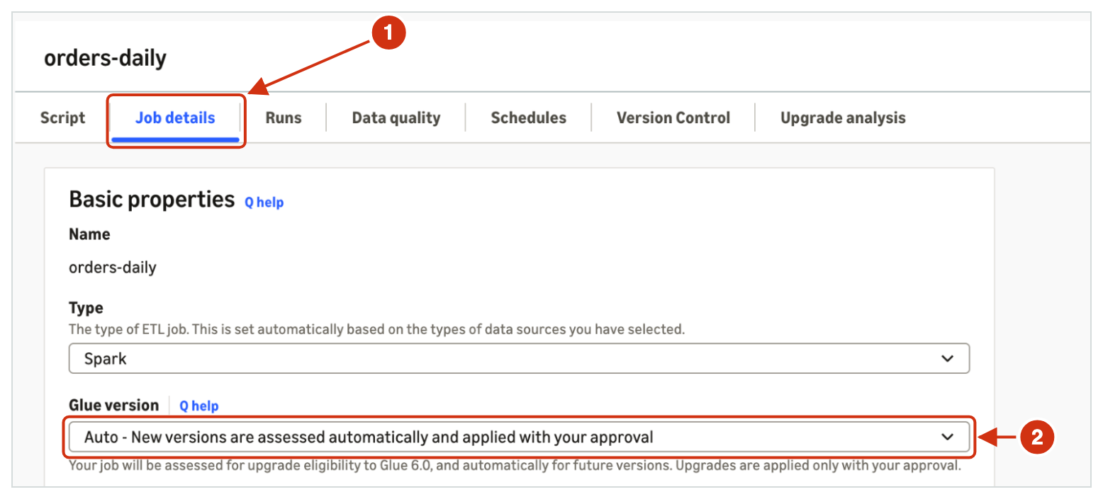
Choose the job, and then choose the Job details tab.
For AWS Glue version, choose Auto, and for Number of retries, enter 1 or higher.
Choose Save.
Figure 1: The Job details tab for orders-daily, with AWS Glue version set to Auto
Approve or decline the upgrade
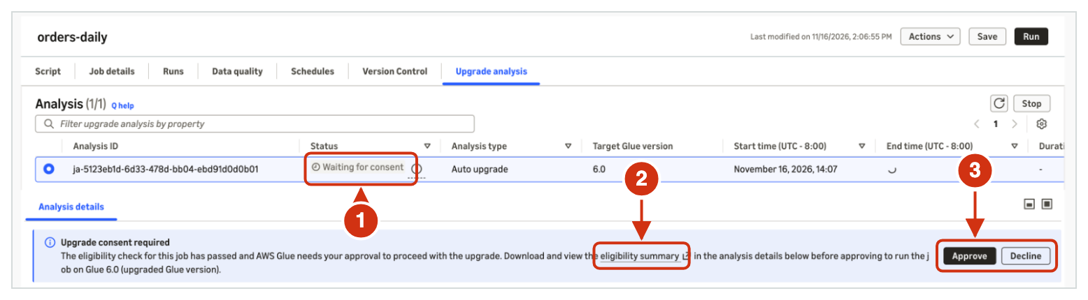
When AWS Glue finishes the compatibility checks and finds no blocking issues, the job waits for your approval.
Choose the job, and then choose the Upgrade analysis tab. The analysis status shows Waiting for consent.
In the Upgrade consent required banner, choose eligibility summary, and review the summary.
Choose Approve to upgrade the job, or choose Decline to keep the job on its current version.
Figure 2: The Upgrade analysis tab for orders-daily, waiting for your approval
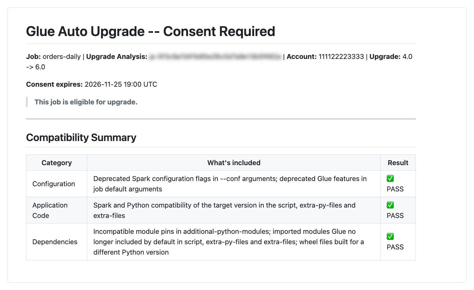
The eligibility summary shows the job, the AWS Glue versions, and the compatibility results.
Figure 3: The eligibility summary for orders-daily
Check the result
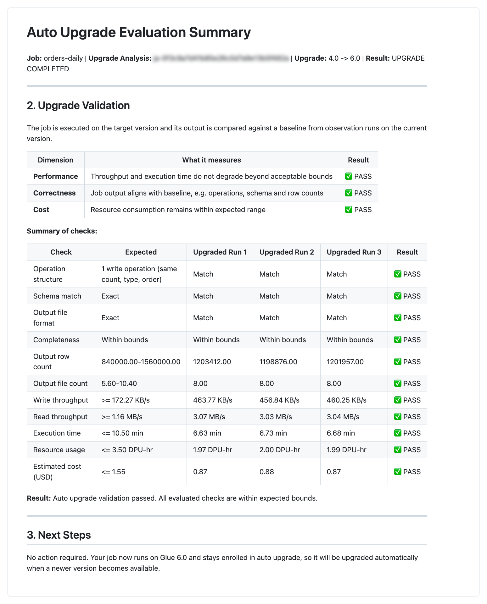
After the evaluation ends, the Upgrade analysis tab shows the auto upgrade evaluation summary. The summary shows the result for performance, correctness, and cost, with the expected range and each upgraded run’s value for every check.
Figure 4: The auto upgrade evaluation summary for orders-daily
Walkthrough: Upgrade a fleet of jobs with an AI agent
When you manage many jobs, an AI agent with the managing-glue-jobs skill assesses, turns on, and approves auto upgrade across your jobs from a few prompts. The agent shows each change and asks for your confirmation before it makes the change.
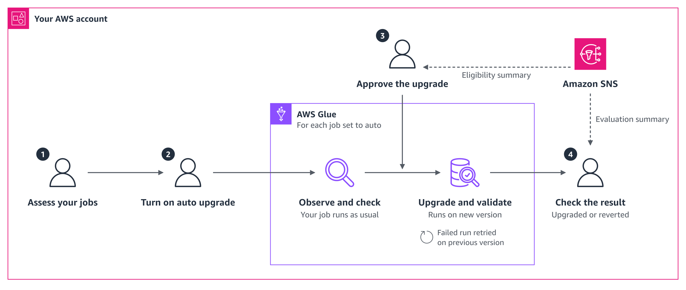
Figure 5: The auto upgrade journey for existing jobs
In this walkthrough, you assess your jobs, turn on auto upgrade, approve the upgrade, and check the result. Between these steps, AWS Glue observes and checks each job, and then upgrades and validates the job. Amazon SNS emails you the eligibility summary and the evaluation summary. The steps that follow match the numbers in Figure 5.
A data team runs three Spark ETL jobs in the US West (Oregon) Region and they want to use AWS Glue version 6.0. The jobs orders-daily and clickstream-agg run on AWS Glue 4.0 and write to Amazon Simple Storage Service (Amazon S3). The job customer-profiles runs on AWS Glue 3.0.
Step 1: Assess your jobs
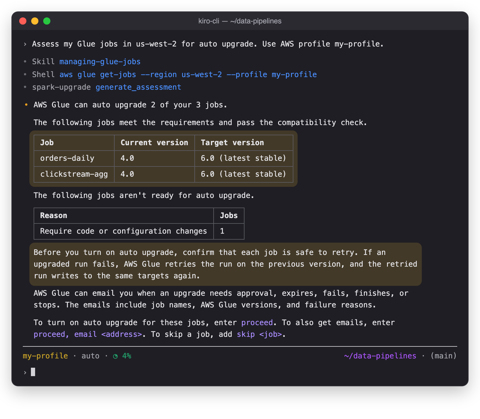
Ask the agent which of your jobs can use auto upgrade. The assessment does not change anything in your environment, so it’s safe to try first. The agent checks each job against the requirements and runs a compatibility assessment. The agent then lists the jobs that can move to AWS Glue 6.0 and asks you to confirm that each job is safe to retry.
Figure 6: The agent assesses the jobs
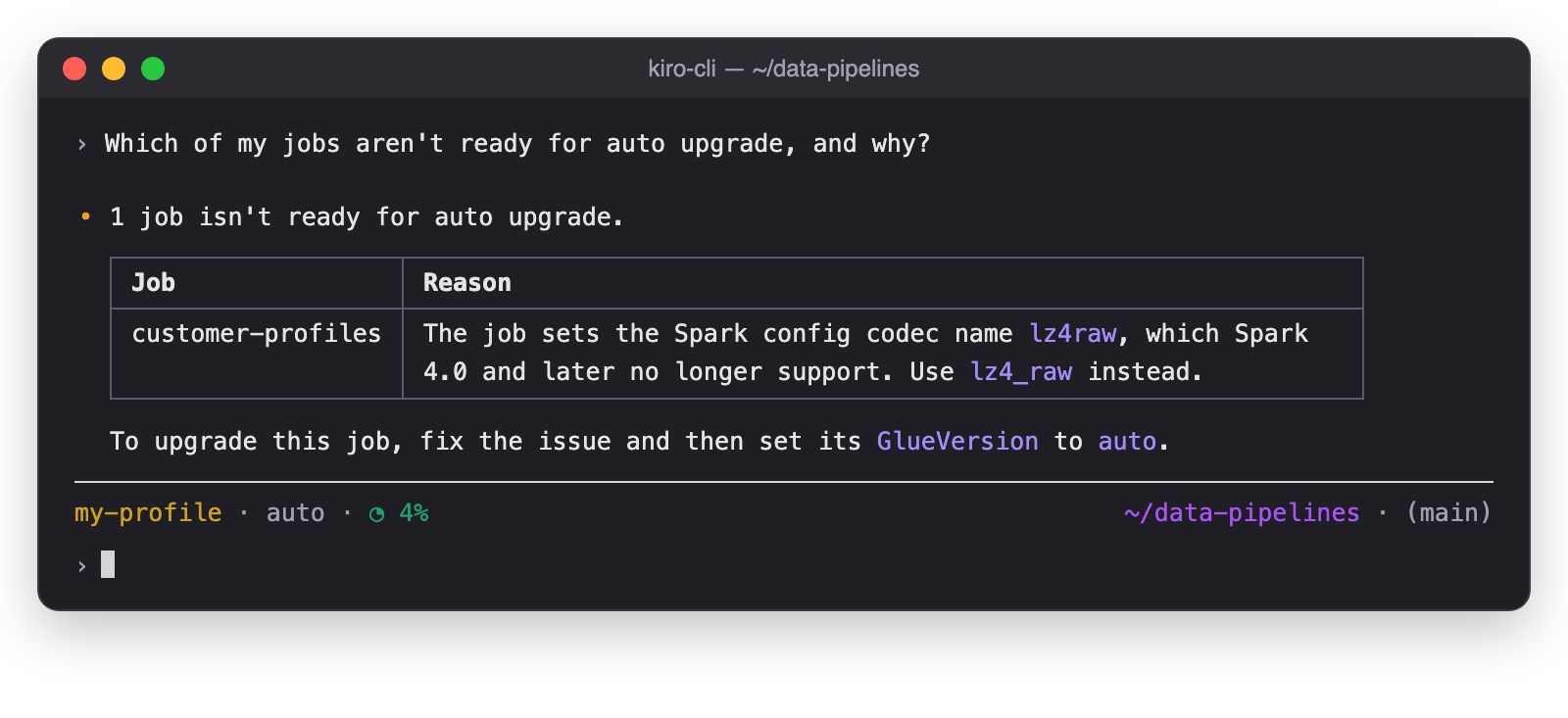
To see which job isn’t ready and why, ask the agent. The agent names the setting that blocks the upgrade and the fix.
Figure 7: The agent explains why a job isn’t ready
Step 2: Turn on auto upgrade and set up email notifications
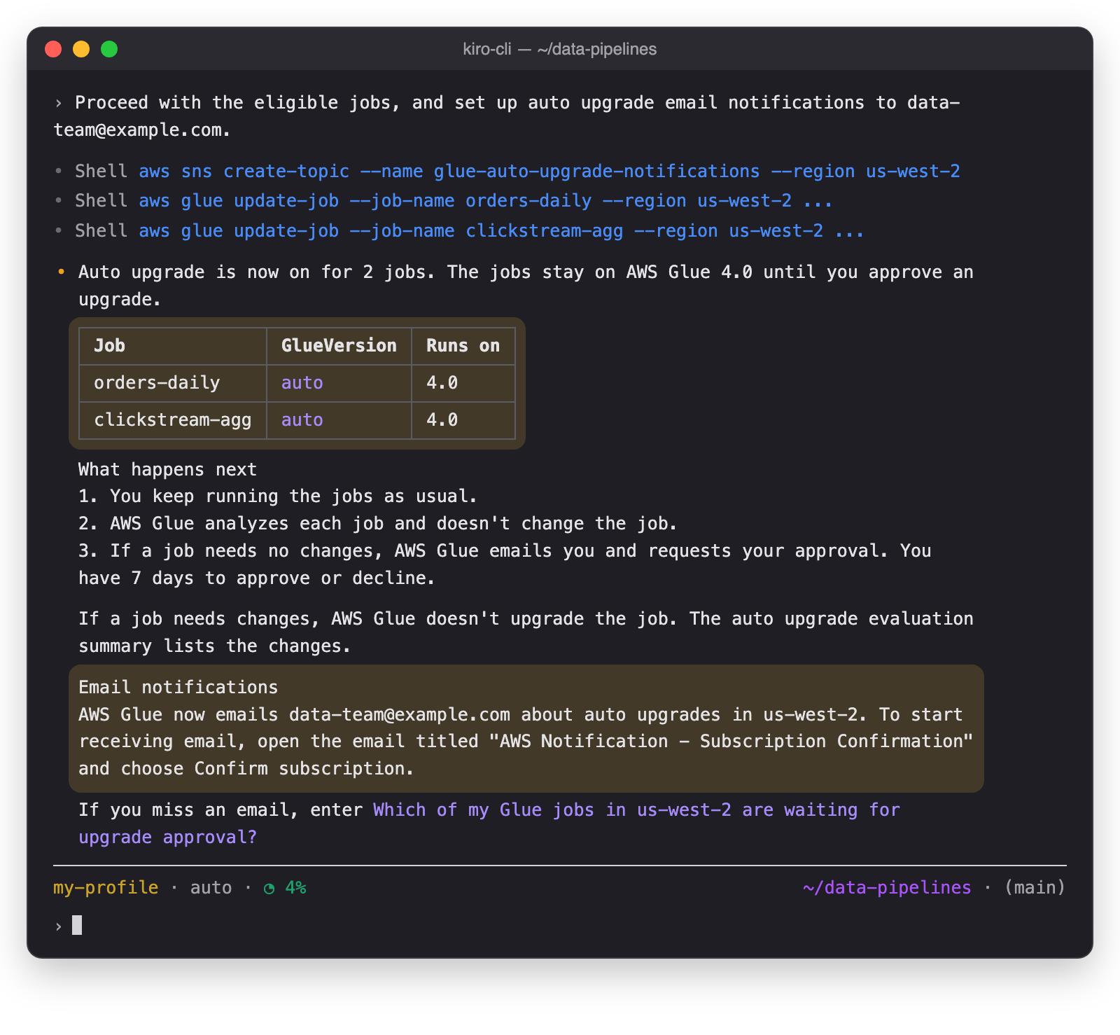
Ask the agent to turn on auto upgrade and set up email notifications in one prompt. The agent sets up the email notifications and sets GlueVersion to auto for each job. The jobs keep running on AWS Glue 4.0 until you approve an upgrade. To get the email notifications, confirm the subscription as the reply describes.
Figure 8: The agent turns on auto upgrade and sets up email notifications
Step 3: Review and approve the upgrade
AWS Glue observes and checks each job in the background, and then you review and approve the upgrade.
Step 3a: AWS Glue observes and checks
You keep running the jobs on their usual schedule. In the background, AWS Glue observes the runs and analyzes each job without changing it. How long this takes depends on how often each job runs.
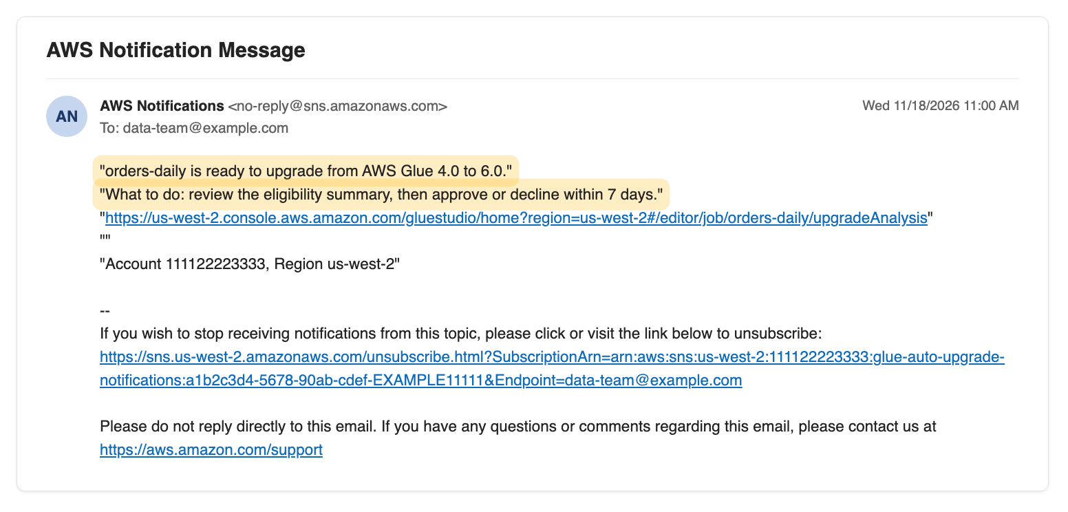
When a job is ready, AWS Glue emails you and requests your approval. The email names the job and the AWS Glue versions, and links to the job in the AWS Glue console. You have seven days to approve or decline.
Figure 9: The approval request email
Step 3b: Review and approve the upgrade
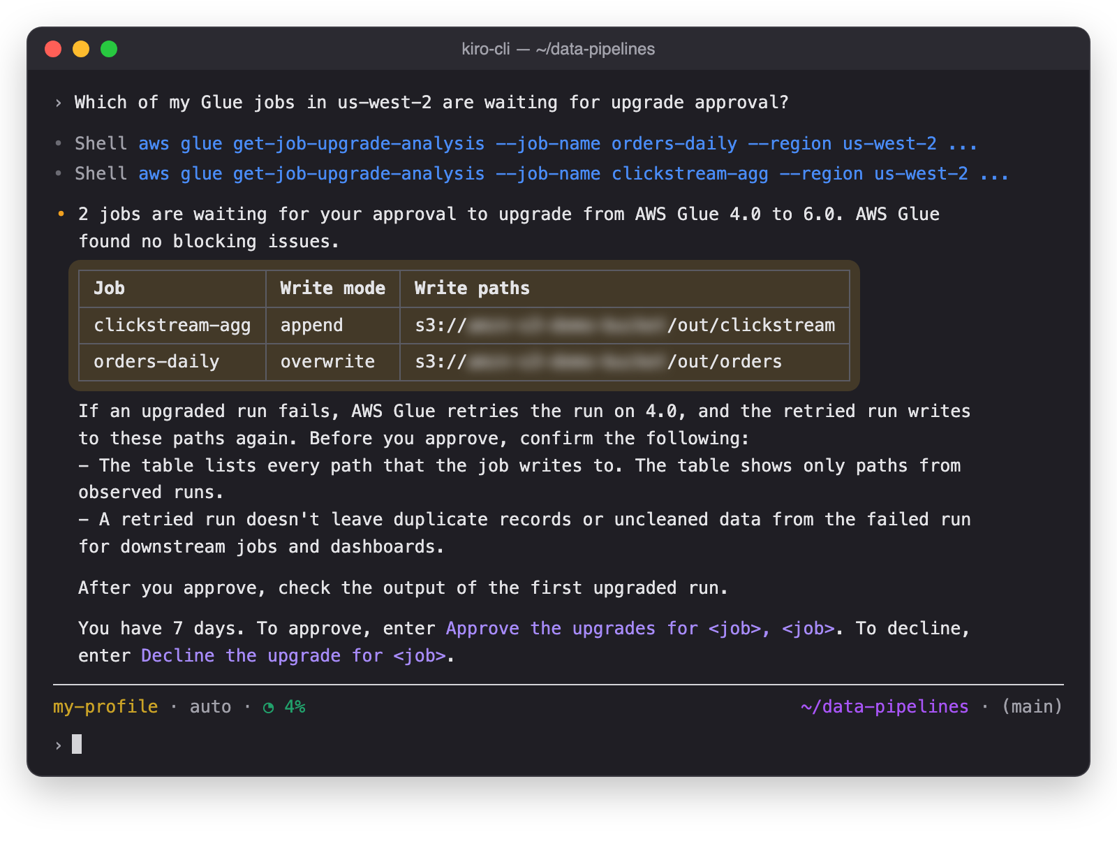
Ask the agent which upgrades are waiting. The agent reads the eligibility summary of each job, and then shows the jobs, their write paths, and what to confirm before you approve.
Figure 10: The agent shows the upgrades that wait for your approval
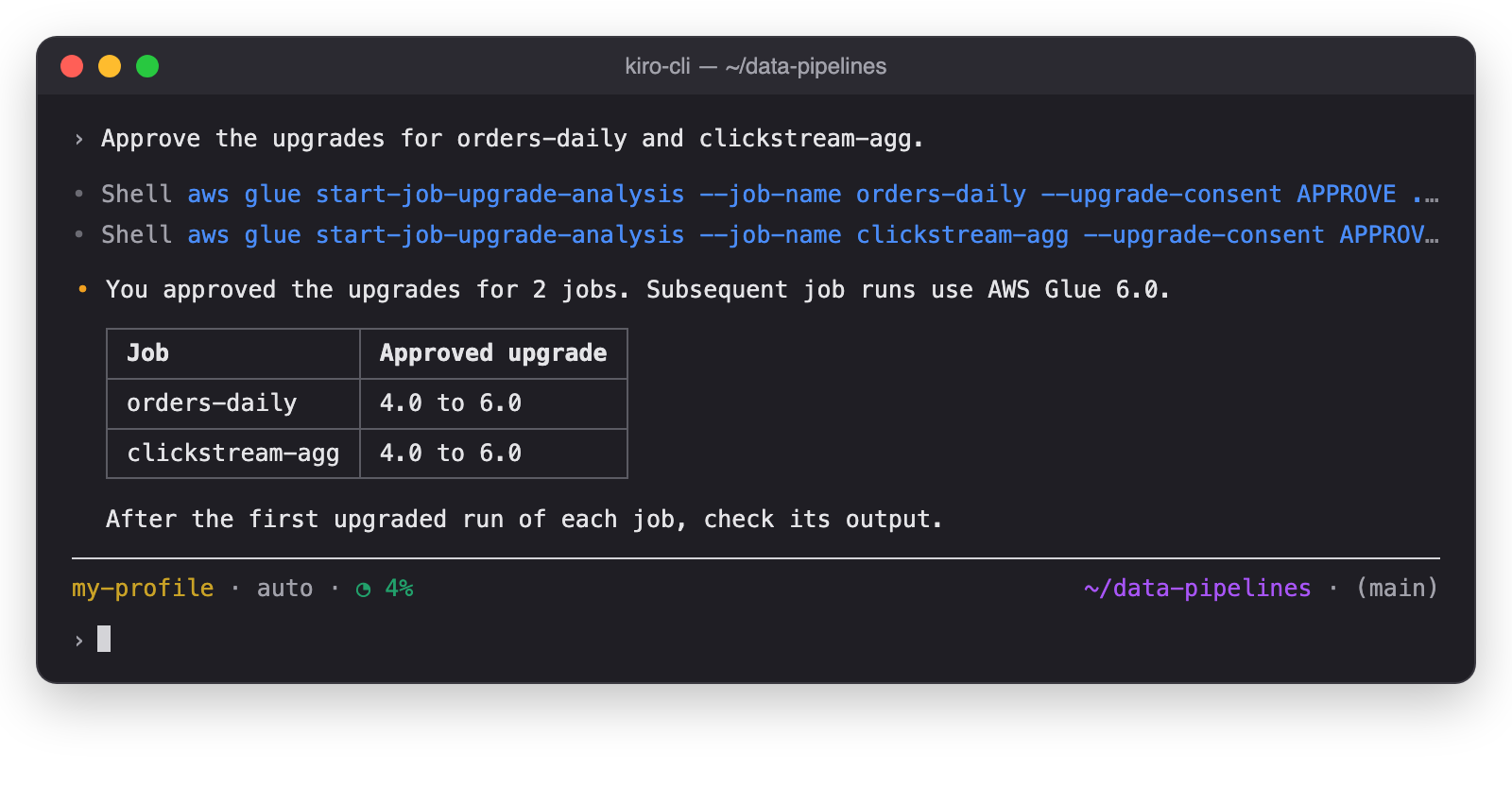
Before you approve, confirm that the reply lists every path that each job writes to. Then approve the jobs in one prompt, and name each job that you approve.
Figure 11: The agent approves the named jobs
The agent approves only the jobs that you name, and only jobs from the review that it showed you.
Step 4: Check the result
AWS Glue upgrades and validates each job, and then you check the result.
Step 4a: AWS Glue upgrades and validates
After you approve, subsequent runs of each job use AWS Glue 6.0, and AWS Glue validates the upgraded runs. If an upgraded run fails, AWS Glue retries the run on AWS Glue 4.0 and reverts the job. You don’t need to act in this step.
Step 4b: Check the result
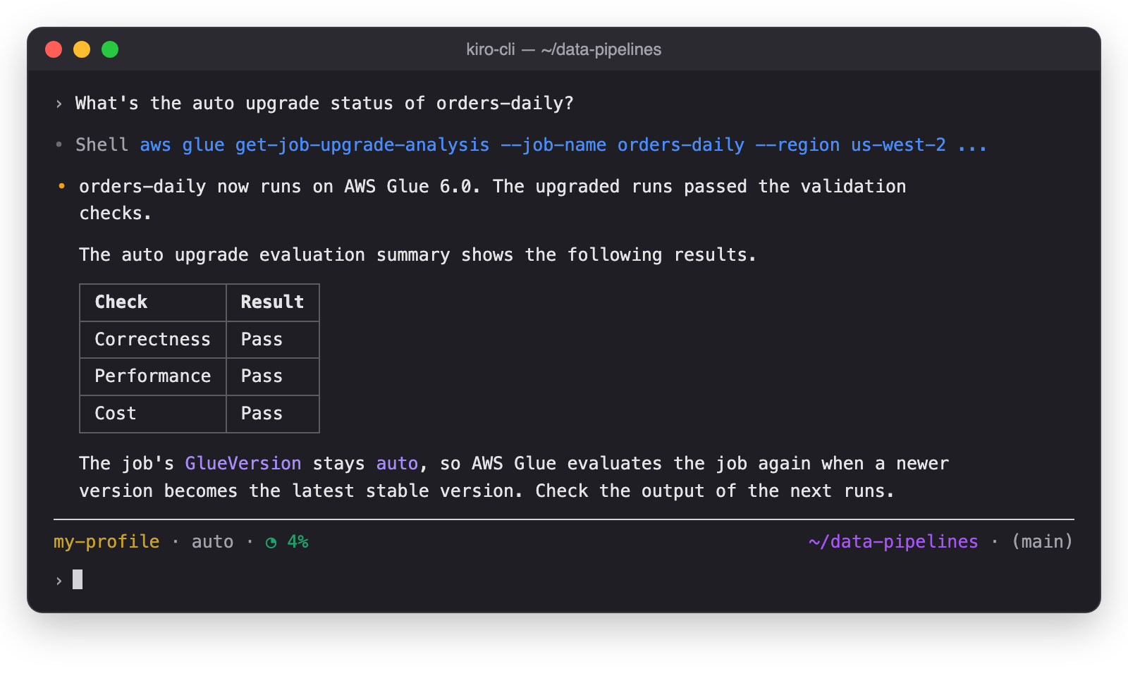
When the evaluation of a job ends, AWS Glue emails you the result. Ask the agent for the result of orders-daily. The agent shows the result of each validation check.
Figure 12: The agent shows the result for orders-daily
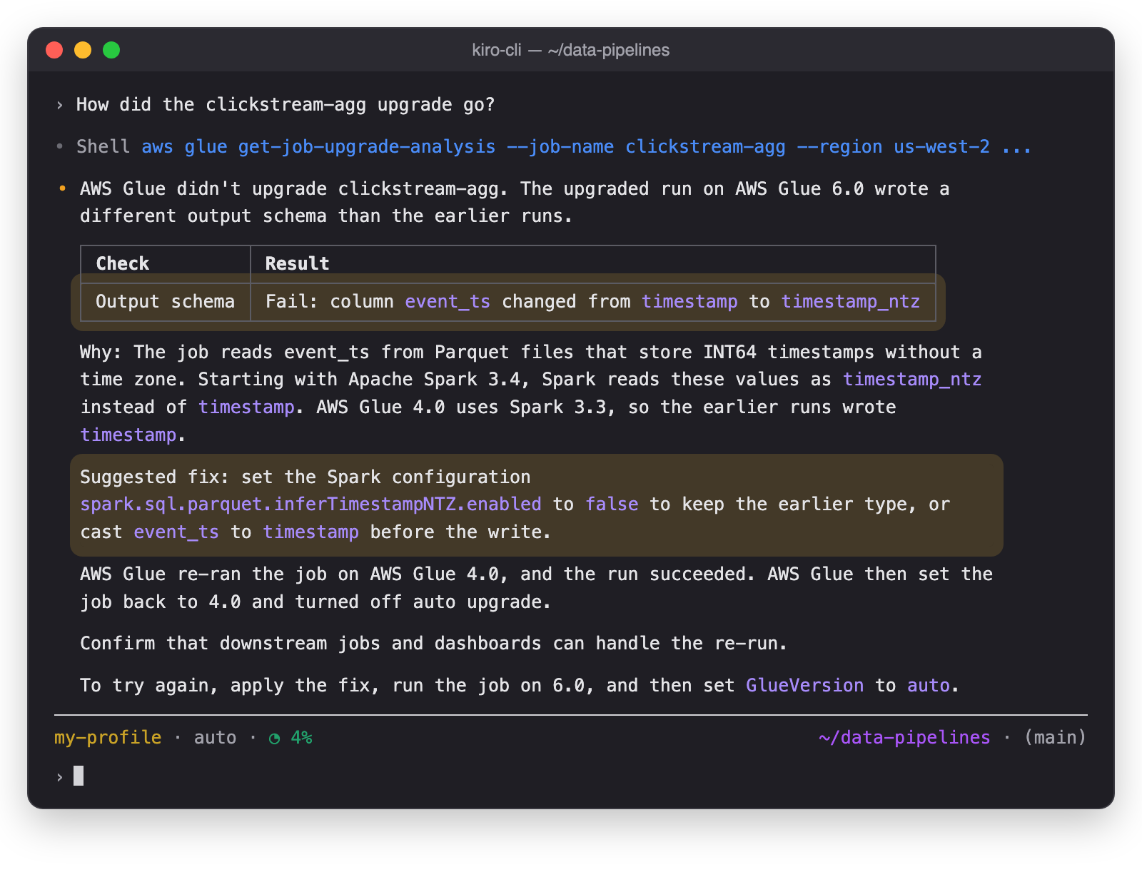
Ask the agent about the other job. The agent shows the check that failed and suggests a fix.
Figure 13: The agent explains why clickstream-agg didn’t upgrade
Your pipeline continues to run on AWS Glue 4.0. The auto upgrade evaluation summary shows what changed, so you can fix the job before you try again.
Conclusion
In this post, we showed how automatic version upgrades for AWS Glue jobs keep your Apache Spark jobs on the latest stable AWS Glue version. You used an AI agent to assess your jobs and turn on auto upgrade with email notifications. You then reviewed the eligibility summary, approved the upgrades, and checked the results in the auto upgrade evaluation summary.
With auto upgrade, your team no longer needs to plan and run an upgrade project for each job. AWS Glue analyzes each job and checks the upgraded runs against the job’s earlier runs. Your team reviews and approves each upgrade. This way you keep your whole fleet of AWS Glue jobs current instead of upgrading one job at a time.
Some jobs need code changes before they can move to a new version. For those jobs, use generative AI upgrades for Apache Spark in AWS Glue, which proposes and validates the code changes for the new version. After you update the code, set the job’s GlueVersion to auto so that AWS Glue keeps the job current from then on.
Auto upgrade is available today in all commercial AWS Regions. For the list of Regions, see Considerations and limitations in the AWS Glue User Guide. To get started, ask an AI agent with the managing-glue-jobs skill to assess the AWS Glue jobs in your account. Try auto upgrade, and share your feedback in the comments.
Special thanks
A special thanks to everyone who contributed from Engineering and Science to the launch of automatic version upgrades: Ezgi Maden, Akshara Ganapathi, Tina Shao, Raghavendhar Thiruvoipadi Vidyasagar, Shoukat Ghouse, David Zhang, Suthan Phillips, Prasad Nadig, Syed Mahmood, Karthik Seshadri, Pradeep Kumar Nalluri, Adam Rohrscheib, Eric Zhang, Tayo Adedokun, Weston Dunn, Kartik Panjabi, Shubham Mehta, Bryan Liles, Steffen Rochel, Kinshuk Pahare, Paul Meighan, and Rick Sears
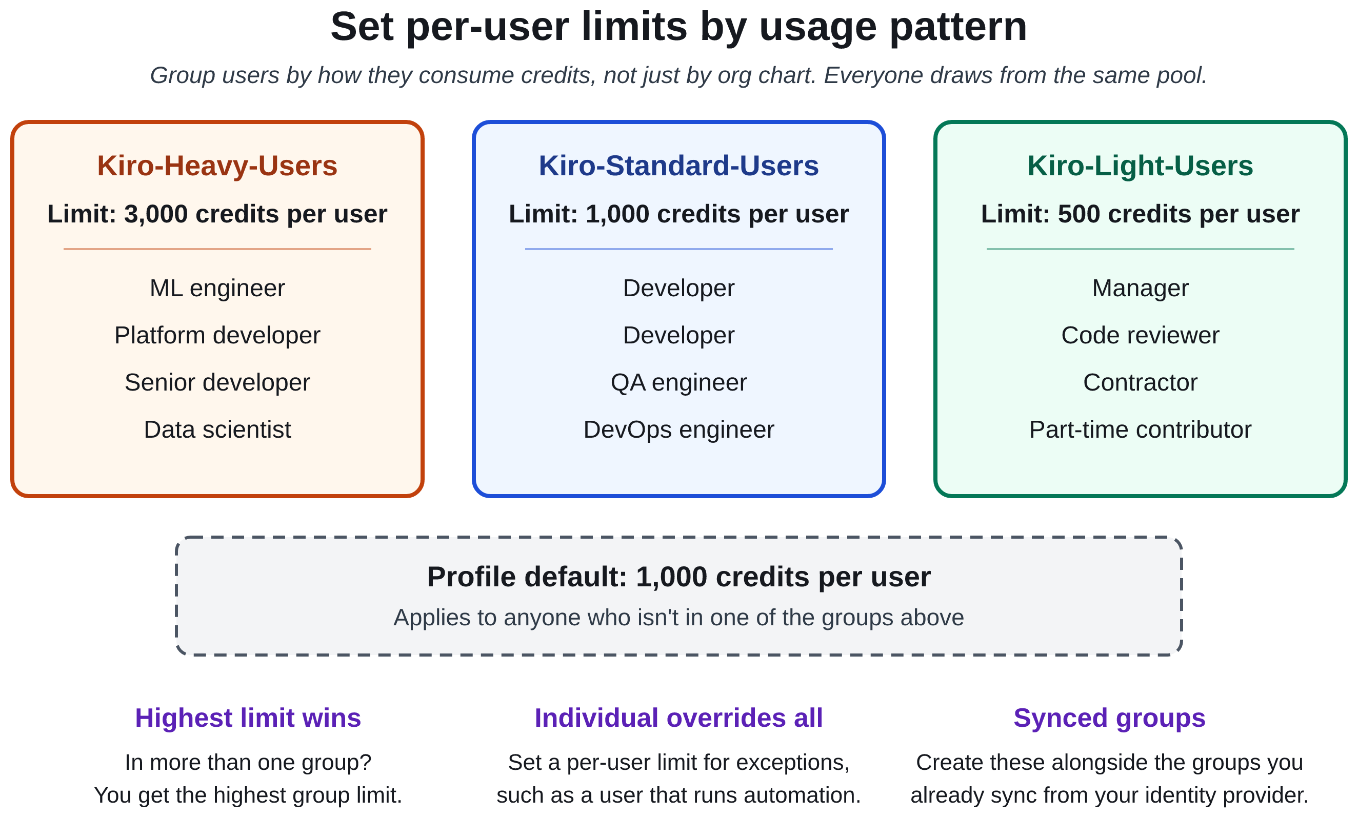
You’ve turned on credit pooling, or you’re about to, and now the decisions are yours: how many seats to keep, how many additional credits to buy, and what limit each developer gets. Set limits too tight and developers get blocked in the middle of a task. Set them too loose and one runaway automation job can drain the pool and pause Kiro for everyone. The data to make these calls is already in your AWS account, in your Kiro user activity reports. This post shows you how to read it.
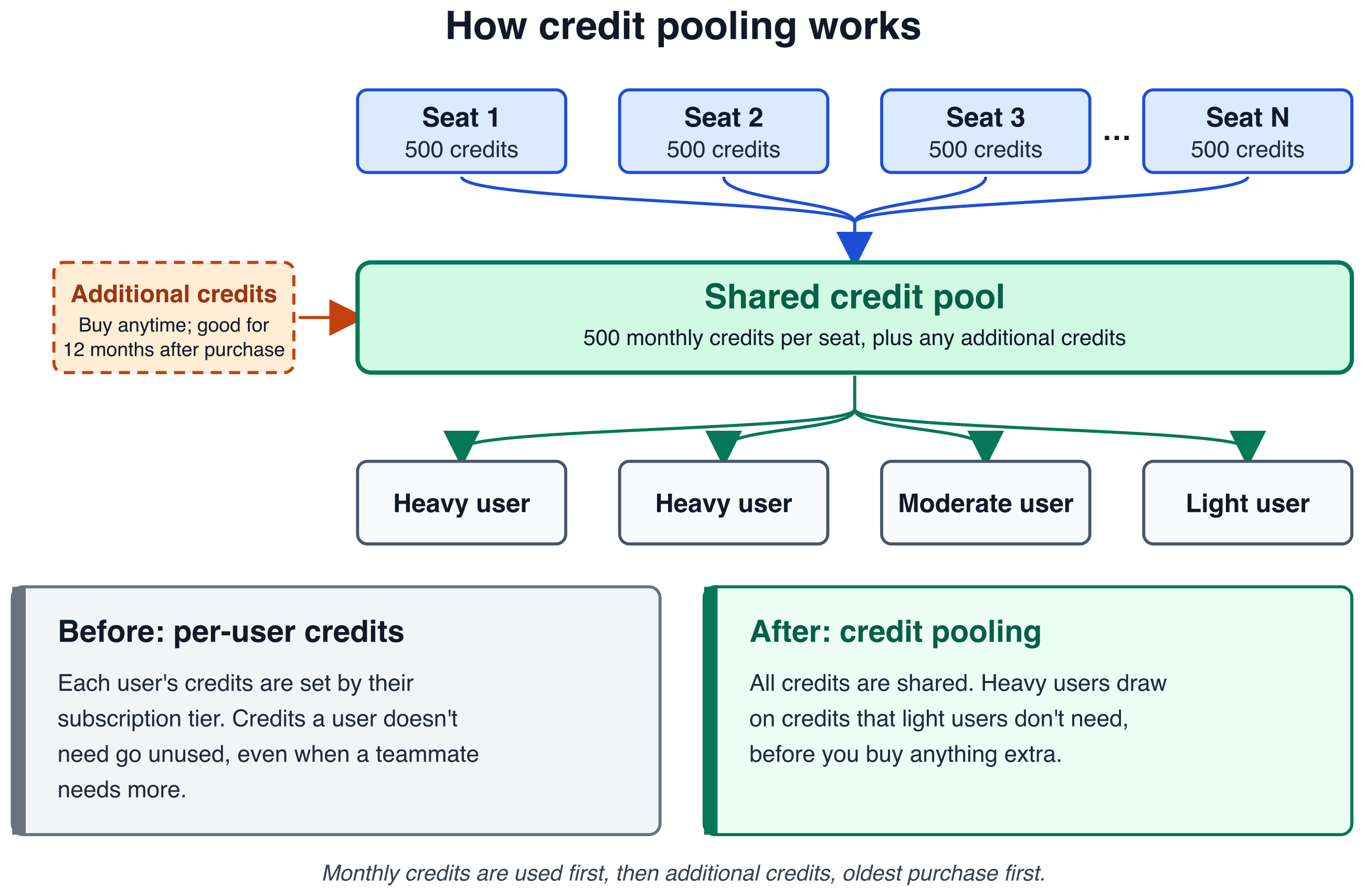
The launch post, Share Kiro credits across your team with credit pooling, published November 4, 2026, introduced credit pooling: a shared pool of Kiro credits that every user in the pool draws from. Credits one developer doesn’t need automatically become available to a teammate who does.
Credit pooling is for organizations. It works with Kiro profiles that use AWS IAM Identity Center, Okta, or Microsoft Entra ID. Individual Kiro subscriptions, such as a personal account with a social login, can’t share credits through a pool, and credit pooling isn’t available in AWS GovCloud (US).
This post is a hands-on guide for admins. It describes how the credit pool behaves day to day and how to size it and dial in your limit settings from your own usage data. It also covers the best practices that keep it running smoothly.
How credit pooling works
In credit pooling, a seat is one user’s access to the pool, and each seat adds 500 monthly credits. When someone leaves, removing them frees their seat for someone else. For details, see Manage seats.
The following diagram shows how each seat’s 500 monthly credit inclusion flows into one shared pool, together with any additional credits you buy, and how every user draws from that pool. It also compares pooling with per-user credits.
Figure 1: How each seat’s 500 monthly credits flow into one shared pool that every user draws from, compared with per-user credits
Here’s a short summary of the core mechanics and how they play out once your pool is running. Each billing cycle, every $20 seat adds 500 credits to the pool, so 100 seats add 50,000. Every seated user draws from the pool, including users that run Kiro in headless mode, such as continuous integration and continuous delivery (CI/CD) pipelines. These credits continue to reset at the end of each billing cycle, but now they’re available for anyone in the pool to use.
When the pool runs out
Admins can buy additional credits at any time in the Kiro console. Additional credits roll over and are good for 12 months after purchase.
Which credits are used first
Monthly credits are used first because they reset at the end of each billing cycle. After the monthly credits run out, Kiro draws from additional credits, starting with the oldest purchase.
Where the savings come from
Credit pooling can help you save in three ways:
Shared credits absorb uneven usage. Your heaviest users draw on credits teammates don’t need before you buy anything extra.
Seats follow your team. Add seats as people join, and remove a user to release their seat when they leave.
Additional credits only when you need them. Buy them at any time, and they roll over for 12 months.
Walkthrough
Today, all you have is a daily report of each user’s consumption. This walkthrough turns that report into a plan in four steps. Step 1 loads the reports into Amazon Athena. Step 2 shows how each month used the pool. Step 3 recommends a seat count and a buffer of additional credits. Step 4 suggests a limit for each user.
Prerequisites
Before you start, confirm that the following are in place.
User activity reports turned on for your Kiro profile. The analysis in this post is based on the daily user activity CSV reports that Kiro writes to an Amazon Simple Storage Service (Amazon S3) bucket. To set them up, including the bucket policy Kiro needs to write to the bucket, see Turn on the CSV report.
Access to Amazon Athena, with permission to read the report location and write query results. For example, attach the AWS managed policy AmazonAthenaFullAccess, and allow s3:GetObject and s3:ListBucket on your report bucket.
The number of seats you bought for a prepaid pool, or the number of users in a postpaid pool. You manage seats under Access management > Credit sharing in the Kiro console. The activity report can’t give you this number.
An administrator role with the credit pooling permissions, so you can change seats, limits, and additional credits after the analysis.
Right-size your pool from your usage data
Your per-user activity reports record each user’s consumption.
Where to start depends on whether you already have data. If your team already uses Kiro, the activity report has recorded every user’s consumption all along, and the following queries run on that history as-is. Run Steps 2 and 3 now, before you pick a seat count. Step 3 tells you what that count needs to be.
If you are new to Kiro, there is nothing to analyze. Buy one seat for each person who needs access. That is the license, and the pool follows from it at 500 credits per seat. Keep a small buffer of additional credits (best practice 4), and start with generous limits (best practice 2). Either way, run one full billing cycle on pooling and come back to Step 2.
Step 1: Create the table and view
In the LOCATION line, replace the four capitalized placeholders. Use the Amazon S3 location you chose when you turned on the CSV report.
YOUR-BUCKET: the bucket name from your Amazon S3 location, for example amzn-s3-demo-bucket.
YOUR-PREFIX: the folder after the bucket name, for example user-activity-reports.
ACCOUNT-ID: the 12-digit AWS account where your users are subscribed.
REGION: the Region where you installed your Kiro profile, for example the US East (N. Virginia) Region (us-east-1).
For example, if your S3 location is s3://amzn-s3-demo-bucket/user-activity-reports/, the LOCATION line becomes s3://amzn-s3-demo-bucket/user-activity-reports/AWSLogs/111122223333/KiroLogs/user_report/us-east-1/. Keep the AWSLogs/.../KiroLogs/user_report/ part exactly as written. Kiro creates those folders itself.
Then create the view that the queries in the next steps read from:
CREATE OR REPLACE VIEW kiro_user_activity AS
WITH headers AS (
-- The first row of each report file names its columns.
SELECT "$path" AS report_file,
ARRAY[c1, c2, c3, c4, c5, c6, c7, c8, c9, c10,
c11, c12, c13, c14, c15, c16, c17, c18, c19, c20] AS names
FROM kiro_user_activity_raw
WHERE c1 = 'Date'
),
report_rows AS (
SELECT "$path" AS report_file,
ARRAY[c1, c2, c3, c4, c5, c6, c7, c8, c9, c10,
c11, c12, c13, c14, c15, c16, c17, c18, c19, c20] AS vals
FROM kiro_user_activity_raw
WHERE c1 <> 'Date'
)
-- Pick each value by its column name in that file's header.
-- A column the file doesn't have comes back NULL.
SELECT TRY(vals[array_position(names, 'Date')]) AS report_date,
TRY(vals[array_position(names, 'UserId')]) AS user_id,
TRY(vals[array_position(names, 'Client_Type')]) AS client_type,
TRY(vals[array_position(names, 'Credits_Used')]) AS credits_used,
TRY(vals[array_position(names, 'User_Email')]) AS user_email,
TRY(vals[array_position(names, 'Usage_Limit')]) AS usage_limit,
TRY(vals[array_position(names, 'Subscription_Tier')]) AS subscription_tier
FROM report_rows
JOIN headers USING (report_file);
Three details in that setup are worth knowing:
OpenCSVSerde, not ROW FORMAT DELIMITED. Kiro quotes some fields, and the simpler row format leaves the quote marks on, which breaks any join on user id.
The view finds columns by name, not position. Kiro has added columns to the report over time, so a position can hold a different column in an older file. The view reads each file’s header row and picks values by name. A column a file doesn’t have, like usage_limit in older reports, comes back empty.
The table reads the first 20 columns, all as text. They must be text, because the first row of each file holds column names. Everything the queries use is within the first 14 columns, and anything past 20 is ignored. If a column the queries need ever moves past 20, add c21 and up to both the table and the view.
Confirm it worked before going further:
SELECT COUNT(DISTINCT user_id) AS users,
ROUND(SUM(CAST(credits_used AS DOUBLE)), 2) AS credits,
MIN(report_date) AS first_day,
MAX(report_date) AS last_day
FROM kiro_user_activity;
For an example 100-seat team with six months of reports, that returns:
If that returns zero users, the LOCATION prefix is wrong. If user_id values come back wrapped in quote marks, the table was created with ROW FORMAT DELIMITED.
Step 2: Re-run every cycle and let the data correct your estimate
This is the query you come back to each cycle. It returns one row per closed month at today’s seat count, so one run shows your whole history. Change only the seat count. It answers the right-sizing question directly: at the seats I pay for now, which months overflow the pool, and how much sat unused?
WITH
-- ========================= EDIT ME =========================
inputs AS (
SELECT 100 AS seats -- the seats you pay for today, from the console
),
-- ======================= END EDIT ME =======================

-- Closed months only: the current month is not a full billing cycle yet.
per_user_month AS (
SELECT substr(a.report_date, 1, 7) AS month,
a.user_id,
SUM(CAST(a.credits_used AS DOUBLE)) AS credits
FROM kiro_user_activity a
WHERE date(a.report_date) < date_trunc('month', current_date)
GROUP BY substr(a.report_date, 1, 7), a.user_id
),

totals AS (
SELECT month,
COUNT(*) AS active_users,
SUM(credits) AS consumed,
SUM(GREATEST(credits - 500.0, 0)) AS beyond_own_seat,
approx_percentile(credits, 0.50) AS p50,
approx_percentile(credits, 0.90) AS p90,
MAX(credits) AS max_user
FROM per_user_month
GROUP BY month
)

SELECT
t.month,
i.seats,
t.active_users,
GREATEST(i.seats - t.active_users, 0) AS seats_never_used,
ROUND(t.consumed, 0) AS credits_consumed,
ROUND(GREATEST(i.seats * 500.0 - t.consumed, 0), 0) AS pool_credits_unused,
ROUND(GREATEST(i.seats * 500.0 - t.consumed, 0) * 0.04, 2) AS unused_credit_value_usd,
ROUND(t.beyond_own_seat
- GREATEST(t.consumed - i.seats * 500.0, 0), 0) AS credits_covered_by_sharing,
ROUND(GREATEST(t.consumed - i.seats * 500.0, 0), 0) AS additional_credits_needed,
ROUND(i.seats * 20.0
+ GREATEST(t.consumed - i.seats * 500.0, 0) * 0.04, 2) AS estimated_monthly_cost,
ROUND(t.active_users * 20.0
+ GREATEST(t.consumed - t.active_users * 500.0, 0) * 0.04, 2)
AS cost_if_never_used_seats_reclaimed,
ROUND(t.p90, 0) AS p90_credits_per_user,
ROUND(t.max_user, 0) AS max_credits_per_user
FROM totals t CROSS JOIN inputs i
ORDER BY t.month;
Sample output for the same team, one column per closed month. The current month is left out because it isn’t a full cycle:
For this team, credits that light users didn’t need covered 7,654 to 13,816 credits of heavier users’ demand every month, so it never bought additional credits. That’s how pooling can work. Even so, 2,000 to 11,700 credits went unused each month and 11 to 21 seats sat idle, which Step 3 turns into a plan.
Read it across, not down. If pool_credits_unused stays large for a couple of cycles, the seats behind it are not a one-off. Reclaim them from people who no longer need access and re-run next month to confirm.
If additional_credits_needed is climbing, buy additional credits earlier in the cycle rather than adding seats (see best practice 7). credits_covered_by_sharing, multiplied by $0.04, estimates what sharing saved you each month. When p90_credits_per_user and max_credits_per_user settle into a stable range, that is your signal to set limits with headroom above them.
seats_never_used counts seats with no activity that month, and cost_if_never_used_seats_reclaimed is your cost if you reclaimed them all. Treat it as a bound, not a target. Step 3 looks across several months before it recommends cuts.
The percentiles are your starting point for limits. p90_credits_per_user reflects your heavy users, and max_credits_per_user is the person who reaches a limit first. With fewer than a few dozen active users, lean on max. Step 4 suggests a limit for each person.
Step 3: Turn the numbers into a resizing plan
Step 2 shows what happened. This query turns that into a plan: seats to keep and reclaim, additional credits to hold, and what the change saves. In the EDIT ME block, set your seat count and how many closed months to look back over. Three months is a sensible default, because one quiet month doesn’t mean a seat is unneeded.
WITH
-- ========================= EDIT ME =========================
inputs AS (
SELECT 100 AS seats, -- the seats you pay for today, from the console
3 AS lookback_months -- closed months to base the plan on
),
-- ======================= END EDIT ME =======================

bounds AS (
SELECT i.seats,
date_trunc('month', current_date) AS this_month,
date_add('month', -i.lookback_months,
date_trunc('month', current_date)) AS since
FROM inputs i
),

-- Everyone who used Kiro since the window started, this month included,
-- needs a seat. Seats nobody used in that time are the ones to reclaim.
users AS (
SELECT COUNT(DISTINCT a.user_id) AS active_users
FROM kiro_user_activity a
CROSS JOIN bounds b
WHERE date(a.report_date) >= b.since
),

-- Credits consumed in each closed month of the window.
months AS (
SELECT substr(a.report_date, 1, 7) AS month,
SUM(CAST(a.credits_used AS DOUBLE)) AS consumed
FROM kiro_user_activity a
CROSS JOIN bounds b
WHERE date(a.report_date) >= b.since
AND date(a.report_date) < b.this_month
GROUP BY substr(a.report_date, 1, 7)
),

-- Never recommend more seats than you have, so every result stays sensible.
sized AS (
SELECT b.seats,
u.active_users,
LEAST(b.seats, u.active_users) AS rec
FROM bounds b
CROSS JOIN users u
),

-- Each window month at today's seats and at the recommended seats, with
-- anything past the pool bought as additional credits.
plan AS (
SELECT s.seats,
s.active_users,
s.rec,
MAX(m.consumed) AS busiest,
AVG(s.seats * 20.0
+ GREATEST(m.consumed - s.seats * 500.0, 0) * 0.04) AS cost_now,
AVG(s.rec * 20.0
+ GREATEST(m.consumed - s.rec * 500.0, 0) * 0.04) AS cost_resized
FROM sized s
CROSS JOIN months m
GROUP BY s.seats, s.active_users, s.rec
)

SELECT
seats,
active_users AS active_users_in_window,
rec AS recommended_seats,
seats - rec AS seats_to_reclaim,
ROUND(busiest, 0) AS busiest_month_credits,
rec * 500 AS recommended_pool_credits,
ROUND(GREATEST(busiest - rec * 500.0, 0), 0) AS additional_credits_to_keep,
ROUND(cost_now, 2) AS avg_monthly_cost_now,
ROUND(cost_resized, 2) AS avg_monthly_cost_resized,
ROUND(cost_now - cost_resized, 2) AS avg_monthly_savings
FROM plan;
Sample output for the same team at 100 seats, looking back over July through September:
recommended_seats is one seat for everyone who used Kiro in the lookback or so far this month, however lightly, and seats_to_reclaim is the rest. The report can’t tell you who joined last week or is on leave, so check the names in the Kiro console before you reclaim anything.
additional_credits_to_keep is how far your busiest month ran past the recommended pool. Keep at least that many additional credits on hand going into each cycle (best practice 4). That’s a balance to hold, not an amount to buy every month, so check what’s already in your pool on the Kiro dashboard and buy only the difference. If Step 2 shows consumption climbing, keep more than this.
The cost columns compare the lookback months at your current seats with their cost at the recommended seats, averaged per month. Each month costs $20 per seat plus $0.04 per credit used beyond the pool, counted in the month it’s used. For this example team, reclaiming 14 idle seats would save about $213.30 a month on average, roughly $2,600 a year if the pattern holds. In July, the busiest month, about $200 of the $280 in seat savings came back as additional credits, which is why the buffer matters.
Step 4: Find users whose limits need to change
Seats and the pool are half of right-sizing. Per-user limits are the other half. This query lists the people whose limit is out of step with what they use. It flags anyone whose busiest month in the lookback reached 80% of their limit, anyone who stayed under 25% of their limit every month, and anyone with no limit set. For each one it suggests a new limit: their busiest month plus 25%, rounded up to the nearest 100 and never below the 500 credits a seat adds to the pool. It only lowers limits for people active in every month of the lookback, so a new joiner isn’t cut after one quiet month. Adjust the thresholds in the EDIT ME block.
WITH
-- ========================= EDIT ME =========================
inputs AS (
SELECT 3 AS lookback_months, -- closed months to look back over
0.80 AS raise_at, -- raise if the busiest month reached 80% of the limit
0.25 AS lower_below, -- lower if every month stayed under 25% of the limit
1.25 AS headroom -- new limit = busiest month plus 25%
),
-- ======================= END EDIT ME =======================

bounds AS (
SELECT date_add('month', -i.lookback_months,
date_trunc('month', current_date)) AS since
FROM inputs i
),

-- Credits per user in each month of the window, this month so far included,
-- so a suggested limit is never below what someone has already used.
per_user_month AS (
SELECT a.user_id,
substr(a.report_date, 1, 7) AS month,
ROUND(SUM(CAST(a.credits_used AS DOUBLE)), 2) AS credits
FROM kiro_user_activity a
CROSS JOIN bounds b
WHERE date(a.report_date) >= b.since
GROUP BY a.user_id, substr(a.report_date, 1, 7)
),

-- Each user's plan, limit and email from their most recent report. On a pool,
-- Usage_Limit is the pool limit (999999 means none is set). On a subscription
-- (Pro, Pro+, Pro Max, Power), it's the tier's monthly credit allowance.
-- If one day has both, the pool row wins. Older reports have no limit
-- column, so the view returns NULL and they're skipped.
latest AS (
SELECT a.user_id,
max_by(a.user_email, a.report_date || IF(upper(a.subscription_tier) = 'POOLING', '1', '0')) AS user_email,
max_by(replace(upper(a.subscription_tier), '_', ''),
a.report_date || IF(upper(a.subscription_tier) = 'POOLING', '1', '0')) AS plan,
max_by(TRY_CAST(a.usage_limit AS DOUBLE),
a.report_date || IF(upper(a.subscription_tier) = 'POOLING', '1', '0')) AS lim
FROM kiro_user_activity a
CROSS JOIN bounds b
WHERE date(a.report_date) >= b.since
AND a.usage_limit IS NOT NULL
AND COALESCE(a.subscription_tier, '') <> ''
GROUP BY a.user_id
),

-- Suggested limit: the busiest month plus headroom, rounded up to the
-- nearest 100, and never below the 500 credits one seat brings to the pool.
-- months_active counts the closed months in the lookback with any use.
scored AS (
SELECT l.user_email,
l.plan,
COALESCE(l.lim, 999999) AS lim,
MAX(m.credits) AS busiest,
COUNT_IF(m.month < date_format(current_date, '%Y-%m')) AS months_active,
GREATEST(ceiling(MAX(m.credits) * i.headroom / 100) * 100, 500) AS new_limit,
i.lookback_months,
i.raise_at,
i.lower_below
FROM per_user_month m
JOIN latest l ON m.user_id = l.user_id
CROSS JOIN inputs i
GROUP BY l.user_id, l.user_email, l.plan, l.lim,
i.lookback_months, i.headroom, i.raise_at, i.lower_below
),

-- Lower a limit only for someone who used Kiro in every closed month of the
-- lookback, so a new joiner or someone back from leave isn't cut after one
-- quiet month.
flagged AS (
SELECT *,
CASE
WHEN plan <> 'POOLING' THEN 'limit when pooled'
WHEN lim >= 999999 THEN 'set limit'
WHEN busiest >= raise_at * lim THEN 'raise'
WHEN busiest < lower_below * lim
AND new_limit < lim
AND months_active = lookback_months THEN 'lower'
END AS action
FROM scored
)

SELECT user_email,
CASE plan WHEN 'POOLING' THEN 'Pool' WHEN 'PRO' THEN 'Pro' WHEN 'PROPLUS' THEN 'Pro+'
WHEN 'PROMAX' THEN 'Pro Max' WHEN 'POWER' THEN 'Power' ELSE plan END AS plan,
CAST(ROUND(busiest) AS BIGINT) AS busiest_month,
IF(lim >= 999999, 'none',
CAST(CAST(lim AS BIGINT) AS VARCHAR)) AS usage_limit,
IF(lim >= 999999, NULL,
ROUND(100.0 * busiest / lim, 0)) AS pct_of_limit,
action,
CAST(new_limit AS BIGINT) AS new_limit
FROM flagged
WHERE action IS NOT NULL
ORDER BY CASE action WHEN 'raise' THEN 1 WHEN 'set limit' THEN 2 WHEN 'lower' THEN 3 ELSE 4 END,

user_email;
Sample output for the same team, looking back over July through October so far:
The raise rows are the people closest to being blocked. In their busiest month, user021 used 994 of their 1,000 credits, so one heavy week might stop them. Raising it to 1,300 gives them room. A higher limit adds no cost until the credits are used.
The lower rows are people who use a small share of their limit, like user006, whose busiest month was 513 credits against a 3,000-credit limit. Lowering a limit doesn’t save money, because a credit costs the same whoever uses it. It limits the impact of a runaway automation job, so one person is less likely to drain the pool and block everyone. new_limit is never below what the user has already used this month, so lowering it doesn’t block them right away.
The limit when pooled rows are people still on a Pro, Pro+, Pro Max, or Power subscription. Their usage_limit is the tier’s monthly allowance, so above 100% means they need more than their tier includes, like user091. new_limit is the individual limit to allocate when you add them to the pool. Their usage is already counted in Step 3’s additional_credits_to_keep, so the buffer covers them too.
If several people in one group need the same change, change the group’s limit.
For the exceptions, set new_limit as an individual limit in the Kiro console. It takes priority over group and profile limits (best practice 2). Re-run this query each cycle to catch limits that need to move again.
Best practices for making credit pooling effective
These practices build on the numbers from the walkthrough and help you keep the pool sized without blocking anyone.
1. Learn your usage pattern first
Collect several months of data before you fine-tune anything. A couple of billing cycles show you who your heavy and light users are, how usage rises and falls through a sprint, and how quickly the pool draws down. Once you can see the trend, use the preceding analysis to size the pool and set limits.
2. Use the limit hierarchy strategically
With credit pooling, you can set per-user limits at three levels:
Level
Priority
Use it for
Individual
Highest
Setting a per-user limit that applies to a specific user (for example, a user that runs automations, or someone testing heavily)
Group
Medium
Setting a per-user limit that applies to all members of a group
Profile
Lowest
Setting a default limit applicable to all users
All limits are per-user. There are no aggregate caps at the group or profile level. A group limit sets the per-user cap for everyone in that group.
Where to start: If your team already uses Kiro, start from the limits Step 4 suggests. If you are new to Kiro, start with generous group and profile limits and tighten them after your first billing cycle, only where the data shows you need to. Over-constraining on day one creates friction and support tickets.
3. Group users by usage pattern
Consider grouping users by how they consume credits rather than only by org chart. For example, put heavy users (senior developers, machine learning engineers) in a group with a higher per-user limit, and light users (managers, reviewers) in a group with a lower one.
Figure 2: Grouping users by usage pattern to apply different per-user limits
If you sync groups from your identity provider: Your existing synced groups likely mirror your org chart. Create groups for credit pooling. For example, keep your synced “Engineering” group for access management, but create separate “Kiro-Heavy-Users” and “Kiro-Standard-Users” groups to apply different per-user limits. Users can belong to multiple groups, and the highest limit wins.
4. Keep a buffer of additional credits
When the pool is empty, everyone stops. Watch your pool threshold alerts and buy additional credits before the pool runs low. Because additional credits roll over for 12 months, buying early doesn’t waste them. Step 3’s additional_credits_to_keep shows how many to hold, based on your busiest month.
Daily projected consumption with run-out date predictions.
Credit usage breakdown (monthly compared to additional credits).
Users sharing credits, credits left, and additional credits at a glance.
If you exhaust the monthly pool early, buy additional credits earlier in the cycle. If credits go unused, check whether some seats are inactive (best practice 7).
6. Use notifications to stay ahead
Credit pooling includes built-in alerts that notify admins at 80% and 100% by default:
Pool threshold alerts: Get notified when the pool drops below configured levels.
User usage alerts: Know when individual users approach their limits.
Seat utilization alerts: Know when assigned seats near the number you bought.
Send these to the people who can act on them.
7. Right-size seats, and use credits rather than seats for headroom
A seat is an access license first and a credit contribution second. Treat them as two separate questions.
Seats with zero usage are the first place to look. You pay $20/month for a seat whether anyone signs in or not, and the seats_to_reclaim figure from Step 3 shows how many have gone unused for the whole lookback. Reclaim those from people who no longer need access.
Lightly used seats are a different matter. Don’t cut a license from someone who uses Kiro occasionally because their consumption is low. Their unused credits already go to the pool.
For headroom, buy credits rather than seats. If demand runs ahead of your pool, buy additional credits. Monthly credits reset at the end of the cycle. Additional credits last 12 months.
Things to keep in mind
When the pool runs out, usage stops for everyone in it. Kiro blocks further usage, whatever each user’s limit, until you add credits.
Mid-cycle limit changes take effect immediately. If you lower a user’s limit below their current consumption, they’re blocked right away. If you increase their limit, they can immediately resume their AI use. Plan limit changes at the start of a billing cycle when possible.
In a prepaid pool, seats are billed whether occupied or not. Every seat contributes credits and costs $20/month. Factor in your idle seats when calculating return on investment.
Getting started
If you have a Kiro profile with users signing in through single sign-on (SSO), you’re ready to go:
Switching is irreversible: a user you move can’t go back to an individual subscription. Have each user’s Step 4 limit ready to apply once they’re in the pool.
Key details at a glance
The following table summarizes the numbers and rules covered in this post.
Item
Detail
Credits per seat
500/month (shared)
Cost per seat
$20/month
Additional credits
$0.04 per credit, good for 12 months
Monthly credit reset
End of billing cycle
Consumption order
Monthly → Additional (oldest purchase first)
Limit hierarchy
Individual > Group > Profile
Start sharing
Credit pooling turns unused individual capacity into a shared resource. Teams with uneven usage can get more from the same spend, and limits at every level help you stay in control.
Ready to try it? Head to the Kiro console and turn on credit sharing under Access management. For details on seats, limits, and monitoring, see Credit pooling in the Kiro documentation.
About the authors
The collective thoughts of the interwebz
Manage Consent
To provide the best experiences, we use technologies like cookies to store and/or access device information. Consenting to these technologies will allow us to process data such as browsing behavior or unique IDs on this site. Not consenting or withdrawing consent, may adversely affect certain features and functions.
Functional
Always active
The technical storage or access is strictly necessary for the legitimate purpose of enabling the use of a specific service explicitly requested by the subscriber or user, or for the sole purpose of carrying out the transmission of a communication over an electronic communications network.
Preferences
The technical storage or access is necessary for the legitimate purpose of storing preferences that are not requested by the subscriber or user.
Statistics
The technical storage or access that is used exclusively for statistical purposes.The technical storage or access that is used exclusively for anonymous statistical purposes. Without a subpoena, voluntary compliance on the part of your Internet Service Provider, or additional records from a third party, information stored or retrieved for this purpose alone cannot usually be used to identify you.
Marketing
The technical storage or access is required to create user profiles to send advertising, or to track the user on a website or across several websites for similar marketing purposes.