Post Syndicated from Islam Ghanim original https://aws.amazon.com/blogs/architecture/field-notes-stopping-an-automatically-started-database-instance-with-amazon-rds/
Customers needing to keep an Amazon Relational Database Service (Amazon RDS) instance stopped for more than 7 days, look for ways to efficiently re-stop the database after being automatically started by Amazon RDS. If the database is started and there is no mechanism to stop it; customers start to pay for the instance’s hourly cost. Moreover, customers with database licensing agreements could incur penalties for running beyond their licensed cores/users.
Stopping and starting a DB instance is faster than creating a DB snapshot, and then restoring the snapshot. However, if you plan to keep the Amazon RDS instance stopped for an extended period of time, it is advised to terminate your Amazon RDS instance and recreate it from a snapshot when needed.
This blog provides a step-by-step approach to automatically stop an RDS instance once the auto-restart activity is complete. This saves any costs incurred once the instance is turned on. The proposed architecture is fully serverless and requires no management overhead. It relies on AWS Step Functions and a set of Lambda functions to monitor RDS instance state and stop the instance when required.
Architecture overview
Given the autonomous nature of the architecture and to avoid management overhead, the architecture leverages serverless components.
- The architecture relies on RDS event notifications. Once a stopped RDS instance is started by AWS due to exceeding the maximum time in the stopped state; an event (RDS-EVENT-0154) is generated by RDS.
- The RDS event is pushed to a dedicated SNS topic rds-event-notifications-topic.
- The Lambda function
start-statemachine-execution-lambda is subscribed to the SNS topic rds-event-notifications-topic.
- The function filters messages with event code: RDS-EVENT-0154. In order to restrict the ‘force shutdown’ activity further, the function validates that the RDS instance is tagged with
auto-restart-protection and that the tag value is set to ‘yes’.
- Once all conditions are met, the Lambda function starts the AWS Step Functions state machine execution.
- The AWS Step Functions state machine integrates with two Lambda functions in order to retrieve the instance state, as well as attempt to stop the RDS instance.
- In case the instance state is not ‘available’, the state machine waits for 5 minutes and then re-checks the state.
- Finally, when the Amazon RDS instance state is ‘available’; the state machine will attempt to stop the Amazon RDS instance.

Prerequisites
In order to implement the steps in this post, you need an AWS account as well as an IAM user with permissions to provision and delete resources of the following AWS services:
- Amazon RDS
- AWS Lambda
- AWS Step Functions
- AWS CloudFormation
- AWS SNS
- AWS IAM
Architecture implementation
You can implement the architecture using the AWS Management Console or AWS CLI. For faster deployment, the architecture is available on GitHub. For more information on the repo, visit GitHub.
The steps below explain how to build the end-to-end architecture from within the AWS Management Console:
Create an SNS topic
- Open the Amazon SNS console.
- On the Amazon SNS dashboard, under Common actions, choose Create Topic.
- In the Create new topic dialog box, for Topic name, enter a name for the topic (rds-event-notifications-topic).
- Choose Create topic.
- Note the Topic ARN for the next task (for example, arn:aws:sns:us-east-1:111122223333:my-topic).
Configure RDS event notifications
Amazon RDS uses Amazon Simple Notification Service (Amazon SNS) to provide notification when an Amazon RDS event occurs. These notifications can be in any notification form supported by Amazon SNS for an AWS Region, such as an email, a text message, or a call to an HTTP endpoint.
For this architecture, RDS generates an event indicating that instance has automatically restarted because it exceed the maximum duration to remain stopped. This specific RDS event (RDS-EVENT-0154) belongs to ‘notification’ category. For more information, visit Using Amazon RDS Event Notification.
To subscribe to an RDS event notification
- Sign in to the AWS Management Console and open the Amazon RDS console.
- In the navigation pane, choose Event subscriptions.
- In the Event subscriptions pane, choose Create event subscription.
- In the Create event subscription dialog box, do the following:
- For Name, enter a name for the event notification subscription (
RdsAutoRestartEventSubscription).
- For Send notifications to, choose the SNS topic created in the previous step (
rds-event-notifications-topic).
- For Source type, choose ‘Instances’. Since our source will be RDS instances.
- For Instances to include, choose ‘All instances’. Instances are included or excluded based on the tag, auto-restart-protection. This is to keep the architecture generic and to avoid regular configurations moving forward.
- For Event categories to include, choose ‘Select specific event categories’.
- For Specific event, choose ‘notification’. This is the category under which the RDS event of interest falls. For more information, review Using Amazon RDS Event Notification.
- Choose Create.
- The Amazon RDS console indicates that the subscription is being created.
Create Lambda functions
Following are the three Lambda functions required for the architecture to work:
- start-statemachine-execution-lambda, the function will subscribe to the newly created SNS topic (rds-event-notifications-topic) and starts the AWS Step Functions state machine execution.
- retrieve-rds-instance-state-lambda, the function is triggered by AWS Step Functions state machine to retrieve an RDS instance state (example, available or stopped)
- stop-rds-instance-lambda, the function is triggered by AWS Step Functions state machine in order to attempt to stop an RDS instance.
First, create the Lambda functions’ execution role.
To create an execution role
- Open the roles page in the IAM console.
- Choose Create role.
- Create a role with the following properties.
- Trusted entity – Lambda.
- Permissions – AWSLambdaBasicExecutionRole.
- Role name –
rds-auto-restart-lambda-role.
- The AWSLambdaBasicExecutionRole policy has the permissions that the function needs to write logs to CloudWatch Logs.
Now, create a new policy and attach to the role in order to allow the Lambda function to: start an AWS StepFunctions state machine execution, stop an Amazon RDS instance, retrieve RDS instance status, list tags and add tags.
Use the JSON policy editor to create a policy
- Sign in to the AWS Management Console and open the IAM console.
- In the navigation pane on the left, choose Policies.
- Choose Create policy.
- Choose the JSON tab.
- Paste the following JSON policy document:
{
    "Version": "2012-10-17",
    "Statement": [
        {
            "Sid": "VisualEditor0",
            "Effect": "Allow",
            "Action": [
                "rds:AddTagsToResource",
                "rds:ListTagsForResource",
                "rds:DescribeDBInstances",
                "states:StartExecution",
                "rds:StopDBInstance"
            ],
            "Resource": "*"
        }
    ]
}
- When you are finished, choose Review policy. The Policy Validator reports any syntax errors.
- On the Review policy page, type a Name (
rds-auto-restart-lambda-policy) and a Description (optional) for the policy that you are creating. Review the policy Summary to see the permissions that are granted by your policy. Then choose Create policy to save your work.
To link the new policy to the AWS Lambda execution role
- Sign in to the AWS Management Console and open the IAM console.
- In the navigation pane, choose Policies.
- In the list of policies, select the check box next to the name of the policy to attach. You can use the Filter menu and the search box to filter the list of policies.
- Choose Policy actions, and then choose Attach.
- Select the IAM role created for the three Lambda functions. After selecting the identities, choose Attach policy.
Given the principle of least privilege, it is recommended to create 3 different roles restricting a function’s access to the needed resources only.
Repeat the following step 3 times to create 3 new Lambda functions. Differences between the 3 Lambda functions are: (1) code and (2) triggers:
- Open the Lambda console.
- Choose Create function.
- Configure the following settings:
- Name –
start-statemachine-execution-lambdaretrieve-rds-instance-state-lambdastop-rds-instance-lambda
- Runtime – Python 3.8.
- Role – Choose an existing role.
- Existing role –
rds-auto-restart-lambda-role.
- Choose Create function.
- To configure a test event, choose Test.
- For Event name, enter
test.
- Choose Create.
- For the Lambda function —
start-statemachine-execution-lambda, use the following Python 3.8 sample code:
import json
import boto3
import logging
import os

#Logging
LOGGER = logging.getLogger()
LOGGER.setLevel(logging.INFO)

#Initialise Boto3 for RDS
rdsClient = boto3.client('rds')

def lambda_handler(event, context):

    #log input event
    LOGGER.info("RdsAutoRestart Event Received, now checking if event is eligible. Event Details ==> ", event)

    #Input event from the SNS topic originated from RDS event notifications
    snsMessage = json.loads(event['Records'][0]['Sns']['Message'])
    rdsInstanceId = snsMessage['Source ID']
    stepFunctionInput = {"rdsInstanceId": rdsInstanceId}
    rdsEventId = snsMessage['Event ID']

    #Retrieve RDS instance ARN
    db_instances = rdsClient.describe_db_instances(DBInstanceIdentifier=rdsInstanceId)['DBInstances']
    db_instance = db_instances[0]
    rdsInstanceArn = db_instance['DBInstanceArn']

    # Filter on the Auto Restart RDS Event. Event code: RDS-EVENT-0154.

    if 'RDS-EVENT-0154' in rdsEventId:

        #log input event
        LOGGER.info("RdsAutoRestart Event detected, now verifying that instance was tagged with auto-restart-protection == yes")

        #Verify that instance is tagged with auto-restart-protection tag. The tag is used to classify instances that are required to be terminated once started.

        tagCheckPass = 'false'
        rdsInstanceTags = rdsClient.list_tags_for_resource(ResourceName=rdsInstanceArn)
        for rdsInstanceTag in rdsInstanceTags["TagList"]:
            if 'auto-restart-protection' in rdsInstanceTag["Key"]:
                if 'yes' in rdsInstanceTag["Value"]:
                    tagCheckPass = 'true'
                    #log instance tags
                    LOGGER.info("RdsAutoRestart verified that the instance is tagged auto-restart-protection = yes, now starting the Step Functions Flow")
                else:
                    tagCheckPass = 'false'


        #log instance tags
        LOGGER.info("RdsAutoRestart Event detected, now verifying that instance was tagged with auto-restart-protection == yes")

        if 'true' in tagCheckPass:

            #Initialise StepFunctions Client
            stepFunctionsClient = boto3.client('stepfunctions')

            # Start StepFunctions WorkFlow
            # StepFunctionsArn is stored in an environment variable
            stepFunctionsArn = os.environ['STEPFUNCTION_ARN']
            stepFunctionsResponse = stepFunctionsClient.start_execution(
            stateMachineArn= stepFunctionsArn,
            name=event['Records'][0]['Sns']['MessageId'],
            input= json.dumps(stepFunctionInput)

        )

    else:

        LOGGER.info("RdsAutoRestart Event detected, and event is not eligible")

    return {
            'statusCode': 200
        }
And then, configure an SNS source trigger for the function start-statemachine-execution-lambda. RDS event notifications will be published to this SNS topic:
- In the Designer pane, choose Add trigger.
- In the Trigger configurations pane, select SNS as a trigger.
- For SNS topic, choose the SNS topic previously created (
rds-event-notifications-topic)
- For Enable trigger, keep it checked.
- Choose Add.
- Choose Save.
For the Lambda function — retrieve-rds-instance-state-lambda, use the following Python 3.8 sample code:
import json
import logging
import boto3

#Logging
LOGGER = logging.getLogger()
LOGGER.setLevel(logging.INFO)

#Initialise Boto3 for RDS
rdsClient = boto3.client('rds')


def lambda_handler(event, context):


    #log input event
    LOGGER.info(event)

    #rdsInstanceId is passed as input to the lambda function from the AWS StepFunctions state machine.
    rdsInstanceId = event['rdsInstanceId']
    db_instances = rdsClient.describe_db_instances(DBInstanceIdentifier=rdsInstanceId)['DBInstances']
    db_instance = db_instances[0]
    rdsInstanceState = db_instance['DBInstanceStatus']
    return {
        'statusCode': 200,
        'rdsInstanceState': rdsInstanceState,
        'rdsInstanceId': rdsInstanceId
    }
Choose Save.
For the Lambda function, stop-rds-instance-lambda, use the following Python 3.8 sample code:
import json
import logging
import boto3

#Logging
LOGGER = logging.getLogger()
LOGGER.setLevel(logging.INFO)

#Initialise Boto3 for RDS
rdsClient = boto3.client('rds')


def lambda_handler(event, context):

    #log input event
    LOGGER.info(event)

    rdsInstanceId = event['rdsInstanceId']

    #Stop RDS instance
    rdsClient.stop_db_instance(DBInstanceIdentifier=rdsInstanceId)

    #Tagging


    return {
        'statusCode': 200,
        'rdsInstanceId': rdsInstanceId
    }
Choose Save.
Create a Step Function
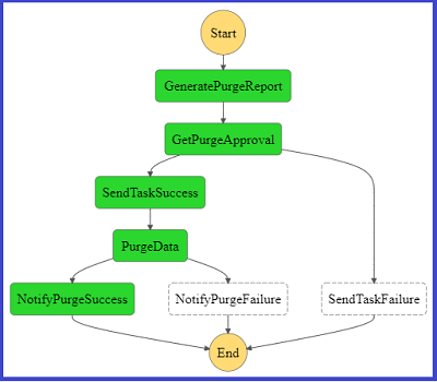
AWS Step Functions will execute the following service logic:
- Retrieve RDS instance state by calling Lambda function,
retrieve-rds-instance-state-lambda. The Lambda function then returns the parameter, rdsInstanceState.
- If the rdsInstanceState parameter value is ‘
available’, then the state machine will step into the next action calling the Lambda function, stop-rds-instance-lambda. If the rdsInstanceState is not ‘available’, the state machine will then wait for 5 minutes and then re-check the RDS instance state again.
- Stopping an RDS instance is an asynchronous operation and accordingly the state machine will keep polling the instance state once every 5 minutes until the
rdsInstanceState parameter value becomes ‘stopped’. Only then, the state machine execution will complete successfully.

- An RDS instance path to ‘available’ state may vary depending on the various maintenance activities scheduled for the instance.
- Once the RDS notification event is generated, the instance will go through multiple states till it becomes ‘available’.
- The use of the 5 minutes timer is to make sure that the automation flow will keep attempting to stop the instance once it becomes available.
- The second part will make sure that the flow doesn’t end till the instance status is changed to ‘stopped’ and hence notifying the system administrator.
To create an AWS Step Functions state machine
- Sign in to the AWS Management Console and open the Amazon RDS console.
- In the navigation pane, choose State machines.
- In the State machines pane, choose Create state machine.
- On the Define state machine page, choose Author with code snippets. For Type, choose Standard.
- Enter a Name for your state machine,
stop-rds-instance-statemachine.
- In the State machine definition pane, add the following state machine definition using the ARNs of the two Lambda function created earlier, as shown in the following code sample:
{
  "Comment": "stop-rds-instance-statemachine: Automatically shutting down RDS instance after a forced Auto-Restart",
  "StartAt": "retrieveRdsInstanceState",
  "States": {
    "retrieveRdsInstanceState": {
      "Type": "Task",
      "Resource": "retrieve-rds-instance-state-lambda Arn",
      "Next": "isInstanceAvailable"
    },
    "isInstanceAvailable": {
      "Type": "Choice",
      "Choices": [
        {
          "Variable": "$.rdsInstanceState",
          "StringEquals": "available",
          "Next": "stopRdsInstance"
        }
      ],
      "Default": "waitFiveMinutes"
    },
    "waitFiveMinutes": {
      "Type": "Wait",
      "Seconds": 300,
      "Next": "retrieveRdsInstanceState"
    },
    "stopRdsInstance": {
      "Type": "Task",
      "Resource": "stop-rds-instance-lambda Arn",
      "Next": "retrieveRDSInstanceStateStopping"
    },
    "retrieveRDSInstanceStateStopping": {
      "Type": "Task",
      "Resource": "retrieve-rds-instance-state-lambda Arn",
      "Next": "isInstanceStopped"
    },
    "isInstanceStopped": {
      "Type": "Choice",
      "Choices": [
        {
          "Variable": "$.rdsInstanceState",
          "StringEquals": "stopped",
          "Next": "notifyDatabaseAdmin"
        }
      ],
      "Default": "waitFiveMinutesStopping"
    },
    "waitFiveMinutesStopping": {
      "Type": "Wait",
      "Seconds": 300,
      "Next": "retrieveRDSInstanceStateStopping"
    },
    "notifyDatabaseAdmin": {
      "Type": "Pass",
      "Result": "World",
      "End": true
    }
  }
}
This is a definition of the state machine written in Amazon States Language which is used to describe the execution flow of an AWS Step Function.
Choose Next.
- In the Name pane, enter a name for your state machine,
stop-rds-instance-statemachine.
- In the Permissions pane, choose Create new role. Take note of the the new role’s name displayed at the bottom of the page (example,
StepFunctions-stop-rds-instance-statemachine-role-231ffecd).
- Choose Create state machine
- By default, the created role only grants the state machine access to CloudWatch logs. Since the state machine will have to make Lambda calls, then another IAM policy has to be associated with the new role.
Use the JSON policy editor to create a policy
- Sign in to the AWS Management Console and open the IAM console.
- In the navigation pane on the left, choose Policies.
- Choose Create policy.
- Choose the JSON tab.
- Paste the following JSON policy document:
{
"Version": "2012-10-17",
"Statement": [
{
"Sid": "VisualEditor0",
"Effect": "Allow",
"Action": "lambda:InvokeFunction",
"Resource": "*"
}
]
}
- When you are finished, choose Review policy. The Policy Validator reports any syntax errors.
- On the Review policy page, type a Name
rds-auto-restart-stepfunctions-policy and a Description (optional) for the policy that you are creating. Review the policy Summary to see the permissions that are granted by your policy.
- Choose Create policy to save your work.
To link the new policy to the AWS Step Functions execution role
- Sign in to the AWS Management Console and open the IAM console.
- In the navigation pane, choose Policies.
- In the list of policies, select the check box next to the name of the policy to attach. You can use the Filter menu and the search box to filter the list of policies.
- Choose Policy actions, and then choose Attach.
- Select the IAM role create for the state machine (example,
StepFunctions-stop-rds-instance-statemachine-role-231ffecd). After selecting the identities, choose Attach policy.
Testing the architecture
In order to test the architecture, create a test RDS instance, tag it with auto-restart-protection tag and set the tag value to yes. While the RDS instance is still in creation process, test the Lambda function — start-statemachine-execution-lambda with a sample event that simulates that the instance was started as it exceeded the maximum time to remain stopped (RDS-EVENT-0154).
To invoke a function
- Sign in to the AWS Management Console and open the Lambda console.
- In navigation pane, choose Functions.
- In Functions pane, choose
start-statemachine-execution-lambda.
- In the upper right corner, choose Test.
- In the Configure test event page, choose Create new test event and in Event template, leave the default Hello World option.
    {
    "Records": [
        {
        "EventSource": "aws:sns",
        "EventVersion": "1.0",
        "EventSubscriptionArn": "<RDS Event Subscription Arn>",
        "Sns": {
            "Type": "Notification",
            "MessageId": "10001-2d55da-9a73-5e42d46748c0",
            "TopicArn": "<SNS Topic Arn>",
            "Subject": "RDS Notification Message",
            "Message": "{\"Event Source\":\"db-instance\",\"Event Time\":\"2020-07-09 15:15:03.031\",\"Identifier Link\":\"https://console.aws.amazon.com/rds/home?region=<region>#dbinstance:id=<RDS instance id>\",\"Source ID\":\"<RDS instance id>\",\"Event ID\":\"http://docs.amazonwebservices.com/AmazonRDS/latest/UserGuide/USER_Events.html#RDS-EVENT-0154\",\"Event Message\":\"DB instance started\"}",
            "Timestamp": "2020-07-09T15:15:03.991Z",
            "SignatureVersion": "1",
            "Signature": "YsuM+L6N8rk+pBPBWoWeRcSuYqo/BN5v9D2lyoSg0B0uS46Q8NZZSoZWaIQi25TXfHY3RYXCXF9WbVGXiWa4dJs2Mjg46anM+2j6z9R7BDz0vt25qCrCyWhmWtc7yeETrlwa0jCtR/wxXFFexRwynqlZeDfvQpf/x+KNLrnJlT61WZ2FMTHYs124RwWU8NY3pm1Os0XOIvm8rfv3ywm1ccZfP4rF7Lfn+2EK6a0635Z/5aiyIlldNZxbgRYTODJYroO9INTlF7NPzVV1Y/K0E9aaL/wQgLZNquXQGCAxPFWy5lxJKeyUocOWcG48KJGIBUC36JJaqVdIilbZ9HvxTg==",
            "SigningCertUrl": "https://sns.<region>.amazonaws.com/SimpleNotificationService-a86cb10b4e1f29c941702d737128f7b6.pem",
            "UnsubscribeUrl": "https://sns.<region>.amazonaws.com/?Action=Unsubscribe&SubscriptionArn=<arn>",
            "MessageAttributes": {}
        }
        }
    ]
    }
start-statemachine-execution-lambda uses the SNS MessageId parameter as name for the AWS Step Functions execution. The name field is unique for a certain period of time, accordingly, with every test run the MessageId parameter value must be changed.
- Choose Create and then choose Test. Each user can create up to 10 test events per function. Those test events are not available to other users.
- AWS Lambda executes your function on your behalf. The
handler in your Lambda function receives and then processes the sample event.
- Upon successful execution, view results in the console.
- The Execution result section shows the execution status as succeeded and also shows the function execution results, returned by the
return statement. Following is a sample response of the test execution:

Now, verify the execution of the AWS Step Functions state machine:
- Sign in to the AWS Management Console and open the Amazon RDS console.
- In navigation pane, choose State machines.
- In the State machine pane, choose
stop-rds-instance-statemachine.
- In the Executions pane, choose the execution with the Name value passed in the test event MessageId parameter.
- In the Visual workflow pane, the real-time execution status is displayed:

- Under the Step details tab, all details related to inputs, outputs and exceptions are displayed:

Monitoring
It is recommended to use Amazon CloudWatch to monitor all the components in this architecture. You can use AWS Step Functions to log the state of the execution, inputs and outputs of each step in the flow. So when things go wrong, you can diagnose and debug problems quickly.
Cost
When you build the architecture using serverless components, you pay for what you use with no upfront infrastructure costs. Cost will depend on the number of RDS instances tagged to be protected against an automatic start.
Architectural considerations
This architecture has to be deployed per AWS Account per Region.
Conclusion
The blog post demonstrated how to build a fully serverless architecture that monitors and stops RDS instances restarted by AWS. This helps to avoid falling behind on any required maintenance updates. This architecture helps you save cost incurred by started instances’ running hours and licensing implications. Feel free to submit enhancements to the GitHub repository or provide feedback in the comments.
Field Notes provides hands-on technical guidance from AWS Solutions Architects, consultants, and technical account managers, based on their experiences in the field solving real-world business problems for customers


 Srikanth Sopirala is a Sr. Analytics Specialist Solutions Architect at AWS. He is a seasoned leader with over 20 years of experience, who is passionate about helping customers build scalable data and analytics solutions to gain timely insights and make critical business decisions. In his spare time, he enjoys reading, spending time with his family and road biking.
 Naresh Gautam is a Sr. Analytics Specialist Solutions Architect at AWS. His role is helping customers architect highly available, high-performance, and cost-effective data analytics solutions to empower customers with data-driven decision-making. In his free time, he enjoys meditation and cooking.


 Harsha Tadiparthi is a Specialist Sr. Solutions Architect, AWS Analytics. He enjoys solving complex customer problems in Databases and Analytics and delivering successful outcomes. Outside of work, he loves to spend time with his family, watch movies, and travel whenever possible.
 Harshida Patel is a Specialist Sr. Solutions Architect, Analytics with AWS.


 James Sun is a Senior Solutions Architect with Amazon Web Services. James has over 15 years of experience in information technology. Prior to AWS, he held several senior technical positions at MapR, HP, NetApp, Yahoo, and EMC. He holds a PhD from Stanford University.
 Chinmayi Narasimhadevara is a Solutions Architect with Amazon Web Services. Chinmayi has over 15 years of experience in information technology and has worked with organizations ranging from large enterprises to mid-sized startups. She helps AWS customers leverage the correct mix of AWS services to achieve success for their business goals.


 George Komninos is a Data Lab Solutions Architect at AWS. He helps customers convert their ideas to a production-ready data product. Before AWS, he spent 3 years at Alexa Information domain as a data engineer. Outside of work, George is a football fan and supports the greatest team in the world, Olympiacos Piraeus.
 Sakti Mishra is a Data Lab Solutions Architect at AWS. He helps customers architect data analytics solutions, which gives them an accelerated path towards modernization initiatives. Outside of work, Sakti enjoys learning new technologies, watching movies, and travel.