Post Syndicated from Anouar Zaaber original https://aws.amazon.com/blogs/big-data/how-engie-scales-their-data-ingestion-pipelines-using-amazon-mwaa/
ENGIE—one of the largest utility providers in France and a global player in the zero-carbon energy transition—produces, transports, and deals electricity, gas, and energy services. With 160,000 employees worldwide, ENGIE is a decentralized organization and operates 25 business units with a high level of delegation and empowerment. ENGIE’s decentralized global customer base had accumulated lots of data, and it required a smarter, unique approach and solution to align its initiatives and provide data that is ingestible, organizable, governable, sharable, and actionable across its global business units.
In 2018, the company’s business leadership decided to accelerate its digital transformation through data and innovation by becoming a data-driven company. Yves Le Gélard, chief digital officer at ENGIE, explains the company’s purpose: “Sustainability for ENGIE is the alpha and the omega of everything. This is our raison d’être. We help large corporations and the biggest cities on earth in their attempts to transition to zero carbon as quickly as possible because it is actually the number one question for humanity today.”
ENGIE, as with any other big enterprise, is using multiple extract, transform, and load (ETL) tools to ingest data into their data lake on AWS. Nevertheless, they usually have expensive licensing plans. “The company needed a uniform method of collecting and analyzing data to help customers manage their value chains,” says Gregory Wolowiec, the Chief Technology Officer who leads ENGIE’s data program. ENGIE wanted a free-license application, well integrated with multiple technologies and with a continuous integration, continuous delivery (CI/CD) pipeline to more easily scale all their ingestion process.
ENGIE started using Amazon Managed Workflows for Apache Airflow (Amazon MWAA) to solve this issue and started moving various data sources from on-premise applications and ERPs, AWS services like Amazon Redshift, Amazon Relational Database Service (Amazon RDS), Amazon DynamoDB, external services like Salesforce, and other cloud providers to a centralized data lake on top of Amazon Simple Storage Service (Amazon S3).
Amazon MWAA is used in particular to collect and store harmonized operational and corporate data from different on-premises and software as a service (SaaS) data sources into a centralized data lake. The purpose of this data lake is to create a “group performance cockpit” that enables an efficient, data-driven analysis and thoughtful decision-making by the Engie Management board.
In this post, we share how ENGIE created a CI/CD pipeline for an Amazon MWAA project template using an AWS CodeCommit repository and plugged it into AWS CodePipeline to build, test, and package the code and custom plugins. In this use case, we developed a custom plugin to ingest data from Salesforce based on the Airflow Salesforce open-source plugin.
Solution overview
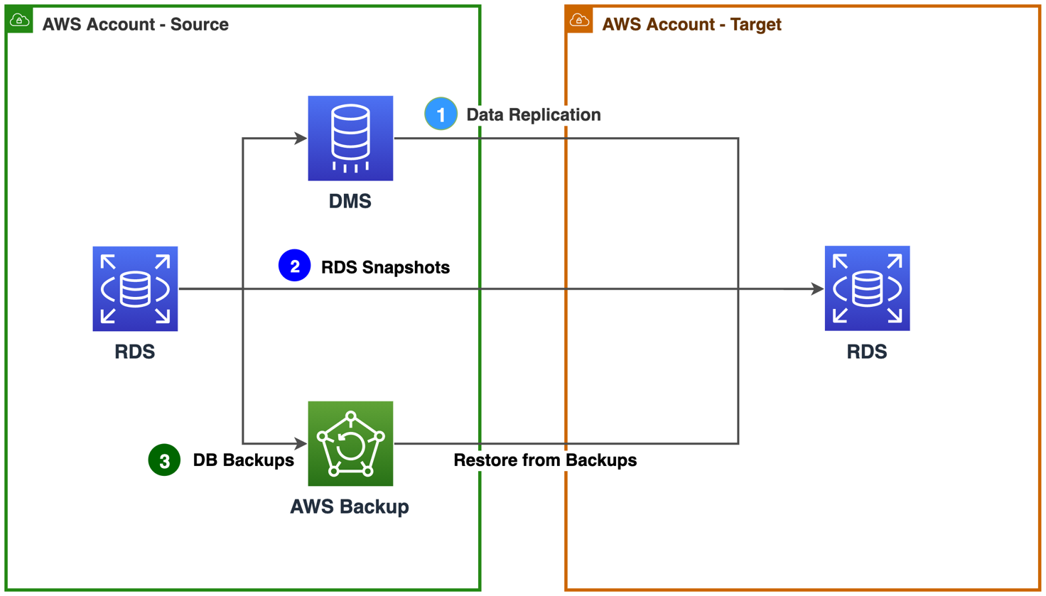
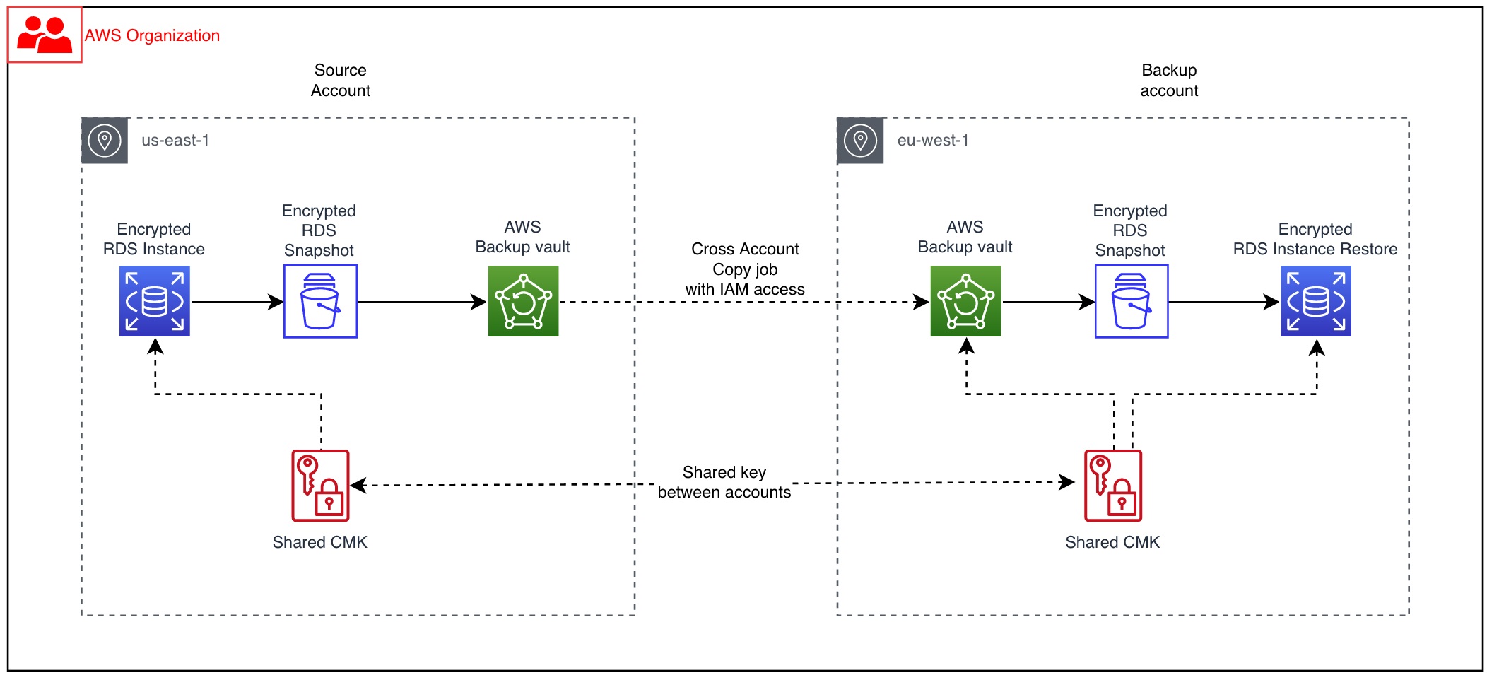
The following diagrams illustrate the solution architecture defining the implemented Amazon MWAA environment and its associated pipelines. It also describes the customer use case for Salesforce data ingestion into Amazon S3.
The following diagram shows the architecture of the deployed Amazon MWAA environment and the implemented pipelines.

The preceding architecture is fully deployed via infrastructure as code (IaC). The implementation includes the following:
- Amazon MWAA environment – A customizable Amazon MWAA environment packaged with plugins and requirements and configured in a secure manner.
- Provisioning pipeline – The admin team can manage the Amazon MWAA environment using the included CI/CD provisioning pipeline. This pipeline includes a CodeCommit repository plugged into CodePipeline to continuously update the environment and its plugins and requirements.
- Project pipeline – This CI/CD pipeline comes with a CodeCommit repository that triggers CodePipeline to continuously build, test and deploy DAGs developed by users. Once deployed, these DAGs are made available in the Amazon MWAA environment.
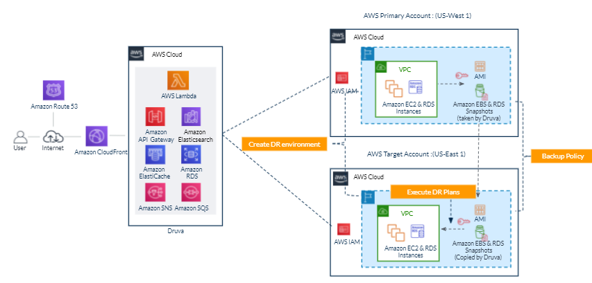
The following diagram shows the data ingestion workflow, which includes the following steps:
- The DAG is triggered by Amazon MWAA manually or based on a schedule.
- Amazon MWAA initiates data collection parameters and calculates batches.
- Amazon MWAA distributes processing tasks among its workers.
- Data is retrieved from Salesforce in batches.
- Amazon MWAA assumes an AWS Identity and Access Management (IAM) role with the necessary permissions to store the collected data into the target S3 bucket.

This AWS Cloud Development Kit (AWS CDK) construct is implemented with the following security best practices:
- With the principle of least privilege, you grant permissions to only the resources or actions that users need to perform tasks.
- S3 buckets are deployed with security compliance rules: encryption, versioning, and blocking public access.
- Authentication and authorization management is handled with AWS Single Sign-On (AWS SSO).
- Airflow stores connections to external sources in a secure manner either in Airflow’s default secrets backend or an alternative secrets backend such as AWS Secrets Manager or AWS Systems Manager Parameter Store.
For this post, we step through a use case using the data from Salesforce to ingest it into an ENGIE data lake in order to transform it and build business reports.
Prerequisites for deployment
For this walkthrough, the following are prerequisites:
- Basic knowledge of the Linux operating system
- Access to an AWS account with administrator or power user (or equivalent) IAM role policies attached
- Access to a shell environment or optionally with AWS CloudShell
Deploy the solution
To deploy and run the solution, complete the following steps:
- Install AWS CDK.
- Bootstrap your AWS account.
- Define your AWS CDK environment variables.
- Deploy the stack.
Install AWS CDK
The described solution is fully deployed with AWS CDK.
AWS CDK is an open-source software development framework to model and provision your cloud application resources using familiar programming languages. If you want to familiarize yourself with AWS CDK, the AWS CDK Workshop is a great place to start.
Install AWS CDK using the following commands:
npm install -g aws-cdk
# To check the installation
cdk --version
Bootstrap your AWS account
First, you need to make sure the environment where you’re planning to deploy the solution to has been bootstrapped. You only need to do this one time per environment where you want to deploy AWS CDK applications. If you’re unsure whether your environment has been bootstrapped already, you can always run the command again:
cdk bootstrap aws://YOUR_ACCOUNT_ID/YOUR_REGION
Define your AWS CDK environment variables
On Linux or MacOS, define your environment variables with the following code:
export CDK_DEFAULT_ACCOUNT=YOUR_ACCOUNT_ID
export CDK_DEFAULT_REGION=YOUR_REGION
On Windows, use the following code:
setx CDK_DEFAULT_ACCOUNT YOUR_ACCOUNT_ID
setx CDK_DEFAULT_REGION YOUR_REGION
Deploy the stack
By default, the stack deploys a basic Amazon MWAA environment with the associated pipelines described previously. It creates a new VPC in order to host the Amazon MWAA resources.
The stack can be customized using the parameters listed in the following table.
To pass a parameter to the construct, you can use the AWS CDK runtime context. If you intend to customize your environment with multiple parameters, we recommend using the cdk.json context file with version control to avoid unexpected changes to your deployments. Throughout our example, we pass only one parameter to the construct. Therefore, for the simplicity of the tutorial, we use the the --context or -c option to the cdk command, as in the following example:
cdk deploy -c paramName=paramValue -c paramName=paramValue ...
| Parameter |
Description |
Default |
Valid values |
| vpcId |
VPC ID where the cluster is deployed. If none, creates a new one and needs the parameter cidr in that case. |
None |
VPC ID |
| cidr |
The CIDR for the VPC that is created to host Amazon MWAA resources. Used only if the vpcId is not defined. |
172.31.0.0/16 |
IP CIDR |
| subnetIds |
Comma-separated list of subnets IDs where the cluster is deployed. If none, looks for private subnets in the same Availability Zone. |
None |
Subnet IDs list (coma separated) |
| envName |
Amazon MWAA environment name |
MwaaEnvironment |
String |
| envTags |
Amazon MWAA environment tags |
None |
See the following JSON example: '{"Environment":"MyEnv", "Application":"MyApp", "Reason":"Airflow"}' |
| environmentClass |
Amazon MWAA environment class |
mw1.small |
mw1.small, mw1.medium, mw1.large |
| maxWorkers |
Amazon MWAA maximum workers |
1 |
int |
| webserverAccessMode |
Amazon MWAA environment access mode (private or public) |
PUBLIC_ONLY |
PUBLIC_ONLY, PRIVATE_ONLY |
| secretsBackend |
Amazon MWAA environment secrets backend |
Airflow |
SecretsManager |
Clone the GitHub repository:
git clone https://github.com/aws-samples/cdk-amazon-mwaa-cicd
Deploy the stack using the following command:
cd mwaairflow && \
pip install . && \
cdk synth && \
cdk deploy -c vpcId=YOUR_VPC_ID
The following screenshot shows the stack deployment:

The following screenshot shows the deployed stack:

Create solution resources
For this walkthrough, you should have the following prerequisites:
If you don’t have a Salesforce account, you can create a SalesForce developer account:
- Sign up for a developer account.
- Copy the host from the email that you receive.
- Log in into your new Salesforce account
- Choose the profile icon, then Settings.
- Choose Reset my Security Token.
- Check your email and copy the security token that you receive.
After you complete these prerequisites, you’re ready to create the following resources:
- An S3 bucket for Salesforce output data
- An IAM role and IAM policy to write the Salesforce output data on Amazon S3
- A Salesforce connection on the Airflow UI to be able to read from Salesforce
- An AWS connection on the Airflow UI to be able to write on Amazon S3
- An Airflow variable on the Airflow UI to store the name of the target S3 bucket
Create an S3 bucket for Salesforce output data
To create an output S3 bucket, complete the following steps:
- On the Amazon S3 console, choose Create bucket.
The Create bucket wizard opens.
- For Bucket name, enter a DNS-compliant name for your bucket, such as
airflow-blog-post.
- For Region, choose the Region where you deployed your Amazon MWAA environment, for example, US East (N. Virginia) us-east-1.
- Choose Create bucket.
For more information, see Creating a bucket.
Create an IAM role and IAM policy to write the Salesforce output data on Amazon S3
In this step, we create an IAM policy that allows Amazon MWAA to write on your S3 bucket.
- On the IAM console, in the navigation pane, choose Policies.
- Choose Create policy.
- Choose the JSON tab.
- Enter the following JSON policy document, and replace
airflow-blog-post with your bucket name:
{
  "Version": "2012-10-17",
  "Statement": [
    {
      "Effect": "Allow",
      "Action": ["s3:ListBucket"],
      "Resource": ["arn:aws:s3:::airflow-blog-post"]
    },
    {
      "Effect": "Allow",
      "Action": [
        "s3:PutObject",
        "s3:GetObject",
        "s3:DeleteObject"
      ],
      "Resource": ["arn:aws:s3:::airflow-blog-post/*"]
    }
  ]
}
- Choose Next: Tags.
- Choose Next: Review.
- For Name, choose a name for your policy (for example,
airflow_data_output_policy).
- Choose Create policy.
Let’s attach the IAM policy to a new IAM role that we use in our Airflow connections.
- On the IAM console, choose Roles in the navigation pane and then choose Create role.
- In the Or select a service to view its use cases section, choose S3.
- For Select your use case, choose S3.
- Search for the name of the IAM policy that we created in the previous step (
airflow_data_output_role) and select the policy.
- Choose Next: Tags.
- Choose Next: Review.
- For Role name, choose a name for your role (
airflow_data_output_role).
- Review the role and then choose Create role.
You’re redirected to the Roles section.
- In the search box, enter the name of the role that you created and choose it.
- Copy the role ARN to use later to create the AWS connection on Airflow.
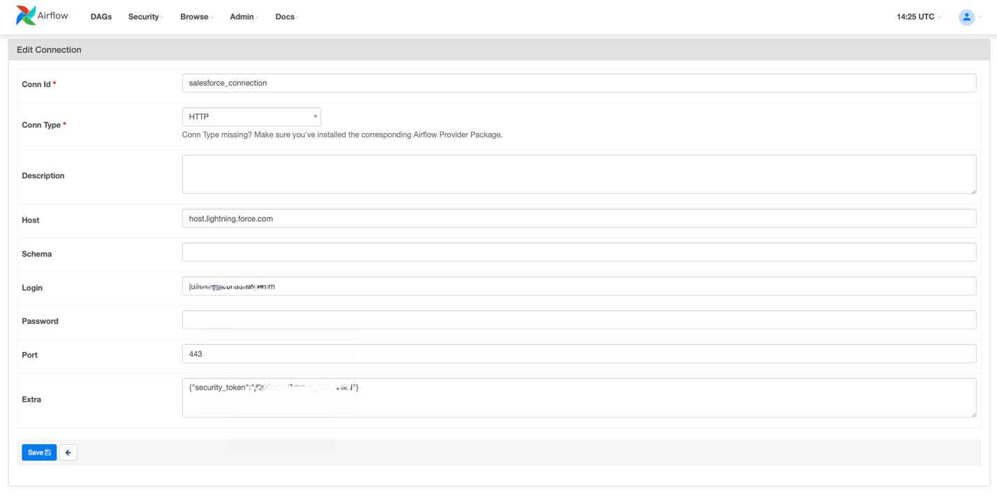
Create a Salesforce connection on the Airflow UI to be able to read from Salesforce
To read data from Salesforce, we need to create a connection using the Airflow user interface.
- On the Airflow UI, choose Admin.
- Choose Connections, and then the plus sign to create a new connection.
- Fill in the fields with the required information.

The following table provides more information about each value.
| Field |
Mandatory |
Description |
Values |
| Conn Id |
Yes |
Connection ID to define and to be used later in the DAG |
For example, salesforce_connection |
| Conn Type |
Yes |
Connection type |
HTTP |
| Host |
Yes |
Salesforce host name |
host-dev-ed.my.salesforce.com or host.lightning.force.com. Replace the host with your Salesforce host and don’t add the http:// as prefix. |
| Login |
Yes |
The Salesforce user name. The user must have read access to the salesforce objects. |
[email protected] |
| Password |
Yes |
The corresponding password for the defined user. |
MyPassword123 |
| Port |
No |
Salesforce instance port. By default, 443. |
443 |
| Extra |
Yes |
Specify the extra parameters (as a JSON dictionary) that can be used in the Salesforce connection. security_token is the Salesforce security token for authentication. To get the Salesforce security token in your email, you must reset your security token. |
{"security_token":"AbCdE..."} |
Create an AWS connection in the Airflow UI to be able to write on Amazon S3
An AWS connection is required to upload data into Amazon S3, so we need to create a connection using the Airflow user interface.
- On the Airflow UI, choose Admin.
- Choose Connections, and then choose the plus sign to create a new connection.
- Fill in the fields with the required information.

The following table provides more information about the fields.
| Field |
Mandatory |
Description |
Value |
| Conn Id |
Yes |
Connection ID to define and to be used later in the DAG |
For example, aws_connection |
| Conn Type |
Yes |
Connection type |
Amazon Web Services |
| Extra |
Yes |
It is required to specify the Region. You also need to provide the role ARN that we created earlier. |
{
"region":"eu-west-1",
"role_arn":"arn:aws:iam::123456789101:role/airflow_data_output_role "
}
|
Create an Airflow variable on the Airflow UI to store the name of the target S3 bucket
We create a variable to set the name of the target S3 bucket. This variable is used by the DAG. So, we need to create a variable using the Airflow user interface.
- On the Airflow UI, choose Admin.
- Choose Variables, then choose the plus sign to create a new variable.

- For Key, enter
bucket_name.
- For Val, enter the name of the S3 bucket that you created in a previous step (
airflow-blog-post).

Create and deploy a DAG in Amazon MWAA
To be able to ingest data from Salesforce into Amazon S3, we need to create a DAG (Directed Acyclic Graph). To create and deploy the DAG, complete the following steps:
- Create a local Python DAG.
- Deploy your DAG using the project CI/CD pipeline.
- Run your DAG on the Airflow UI.
- Display your data in Amazon S3 (with S3 Select).
Create a local Python DAG
The provided SalesForceToS3Operator allows you to ingest data from Salesforce objects to an S3 bucket. Refer to standard Salesforce objects for the full list of objects you can ingest data from with this Airflow operator.
In this use case, we ingest data from the Opportunity Salesforce object. We retrieve the last 6 months’ data in monthly batches and we filter on a specific list of fields.
The DAG provided in the sample in GitHub repository imports the last 6 months of the Opportunity object (one file by month) by filtering the list of retrieved fields.
This operator takes two connections as parameters:
- An AWS connection that is used to upload ingested data into Amazon S3.
- A Salesforce connection to read data from Salesforce.
The following table provides more information about the parameters.
| Parameter |
Type |
Mandatory |
Description |
| sf_conn_id |
string |
Yes |
Name of the Airflow connection that has the following information:
- user name
- password
- security token
|
| sf_obj |
string |
Yes |
Name of the relevant Salesforce object (Account, Lead, Opportunity) |
| s3_conn_id |
string |
Yes |
The destination S3 connection ID |
| s3_bucket |
string |
Yes |
The destination S3 bucket |
| s3_key |
string |
Yes |
The destination S3 key |
| sf_fields |
string |
No |
The (optional) list of fields that you want to get from the object (Id, Name, and so on).
If none (the default), then this gets all fields for the object. |
| fmt |
string |
No |
The (optional) format that the S3 key of the data should be in.
Possible values include CSV (default), JSON, and NDJSON. |
| from_date |
date format |
No |
A specific date-time (optional) formatted input to run queries from for incremental ingestion.
Evaluated against the SystemModStamp attribute.
Not compatible with the query parameter and should be in date-time format (for example, 2021-01-01T00:00:00Z).
Default: None |
| to_date |
date format |
No |
A specific date-time (optional) formatted input to run queries to for incremental ingestion.
Evaluated against the SystemModStamp attribute.
Not compatible with the query parameter and should be in date-time format (for example, 2021-01-01T00:00:00Z).
Default: None |
| query |
string |
No |
A specific query (optional) to run for the given object.
This overrides default query creation.
Default: None |
| relationship_object |
string |
No |
Some queries require relationship objects to work, and these are not the same names as the Salesforce object.
Specify that relationship object here (optional).
Default: None |
| record_time_added |
boolean |
No |
Set this optional value to true if you want to add a Unix timestamp field to the resulting data that marks when the data was fetched from Salesforce.
Default: False |
| coerce_to_timestamp |
boolean |
No |
Set this optional value to true if you want to convert all fields with dates and datetimes into Unix timestamp (UTC).
Default: False |
The first step is to import the operator in your DAG:
from operators.salesforce_to_s3_operator import SalesforceToS3Operator
Then define your DAG default ARGs, which you can use for your common task parameters:
# These args will get passed on to each operator
# You can override them on a per-task basis during operator initialization
default_args = {
    'owner': '[email protected]',
    'depends_on_past': False,
    'start_date': days_ago(2),
    'retries': 0,
    'retry_delay': timedelta(minutes=1),
    'sf_conn_id': 'salesforce_connection',
    's3_conn_id': 'aws_connection',
    's3_bucket': 'salesforce-to-s3',
}
...
Finally, you define the tasks to use the operator.
The following examples illustrate some use cases.
Salesforce object full ingestion
This task ingests all the content of the Salesforce object defined in sf_obj. This selects all the object’s available fields and writes them into the defined format in fmt. See the following code:
...
salesforce_to_s3 = SalesforceToS3Operator(
    task_id="Opportunity_to_S3",
    sf_conn_id=default_args["sf_conn_id"],
    sf_obj="Opportunity",
    fmt="ndjson",
    s3_conn_id=default_args["s3_conn_id"],
    s3_bucket=default_args["s3_bucket"],
    s3_key=f"salesforce/raw/dt={s3_prefix}/{table.lower()}.json",
    dag=salesforce_to_s3_dag,
)
...
Salesforce object partial ingestion based on fields
This task ingests specific fields of the Salesforce object defined in sf_obj. The selected fields are defined in the optional sf_fields parameter. See the following code:
...
salesforce_to_s3 = SalesforceToS3Operator(
    task_id="Opportunity_to_S3",
    sf_conn_id=default_args["sf_conn_id"],
    sf_obj="Opportunity",
    sf_fields=["Id","Name","Amount"],
    fmt="ndjson",
    s3_conn_id=default_args["s3_conn_id"],
    s3_bucket=default_args["s3_bucket"],
    s3_key=f"salesforce/raw/dt={s3_prefix}/{table.lower()}.json",
    dag=salesforce_to_s3_dag,
)
...
Salesforce object partial ingestion based on time period
This task ingests all the fields of the Salesforce object defined in sf_obj. The time period can be relative using from_date or to_date parameters or absolute by using both parameters.
The following example illustrates relative ingestion from the defined date:
...
salesforce_to_s3 = SalesforceToS3Operator(
    task_id="Opportunity_to_S3",
    sf_conn_id=default_args["sf_conn_id"],
    sf_obj="Opportunity",
    from_date="YESTERDAY",
    fmt="ndjson",
    s3_conn_id=default_args["s3_conn_id"],
    s3_bucket=default_args["s3_bucket"],
    s3_key=f"salesforce/raw/dt={s3_prefix}/{table.lower()}.json",
    dag=salesforce_to_s3_dag,
)
...
The from_date and to_date parameters support Salesforce date-time format. It can be either a specific date or literal (for example TODAY, LAST_WEEK, LAST_N_DAYS:5). For more information about date formats, see Date Formats and Date Literals.
For the full DAG, refer to the sample in GitHub repository.
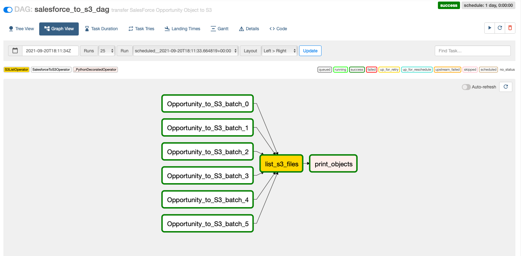
This code dynamically generates tasks that run queries to retrieve the data of the Opportunity object in the form of 1-month batches.
The sf_fields parameter allows us to extract only the selected fields from the object.
Save the DAG locally as salesforce_to_s3.py.
Deploy your DAG using the project CI/CD pipeline
As part of the CDK deployment, a CodeCommit repository and CodePipeline pipeline were created in order to continuously build, test, and deploy DAGs into your Amazon MWAA environment.
To deploy the new DAG, the source code should be committed to the CodeCommit repository. This triggers a CodePipeline run that builds, tests, and deploys your new DAG and makes it available in your Amazon MWAA environment.
- Sign in to the CodeCommit console in your deployment Region.
- Under Source, choose Repositories.
You should see a new repository mwaaproject.
- Push your new DAG in the
mwaaproject repository under dags. You can either use the CodeCommit console or the Git command line to do so:
- CodeCommit console:
- Choose the project CodeCommit repository name
mwaaproject and navigate under dags.
- Choose Add file and then Upload file and upload your new DAG.
- Git command line:
- To be able to clone and access your CodeCommit project with the Git command line, make sure Git client is properly configured. Refer to Setting up for AWS CodeCommit.
- Clone the repository with the following command after replacing <region> with your project Region:
git clone https://git-codecommit.<region>.amazonaws.com/v1/repos/mwaaproject
- Copy the DAG file under
dags and add it with the command:
git add dags/salesforce_to_s3.py
- Commit your new file with a message:
git commit -m "add salesforce DAG"
- Push the local file to the CodeCommit repository:
The new commit triggers a new pipeline that builds, tests, and deploys the new DAG. You can monitor the pipeline on the CodePipeline console.
- On the CodePipeline console, choose Pipeline in the navigation pane.
- On the Pipelines page, you should see
mwaaproject-pipeline.
- Choose the pipeline to display its details.

After checking that the pipeline run is successful, you can verify that the DAG is deployed to the S3 bucket and therefore available on the Amazon MWAA console.
- On the Amazon S3 console, look for a bucket starting with
mwaairflowstack-mwaaenvstackne and go under dags.
You should see the new DAG.
- On the Amazon MWAA console, choose DAGs.
You should be able to see the new DAG.

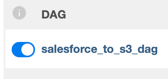
Run your DAG on the Airflow UI
Go to the Airflow UI and toggle on the DAG.

This triggers your DAG automatically.
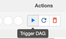
Later, you can continue manually triggering it by choosing the run icon.

Choose the DAG and Graph View to see the run of your DAG.

If you have any issue, you can check the logs of the failed tasks from the task instance context menu.

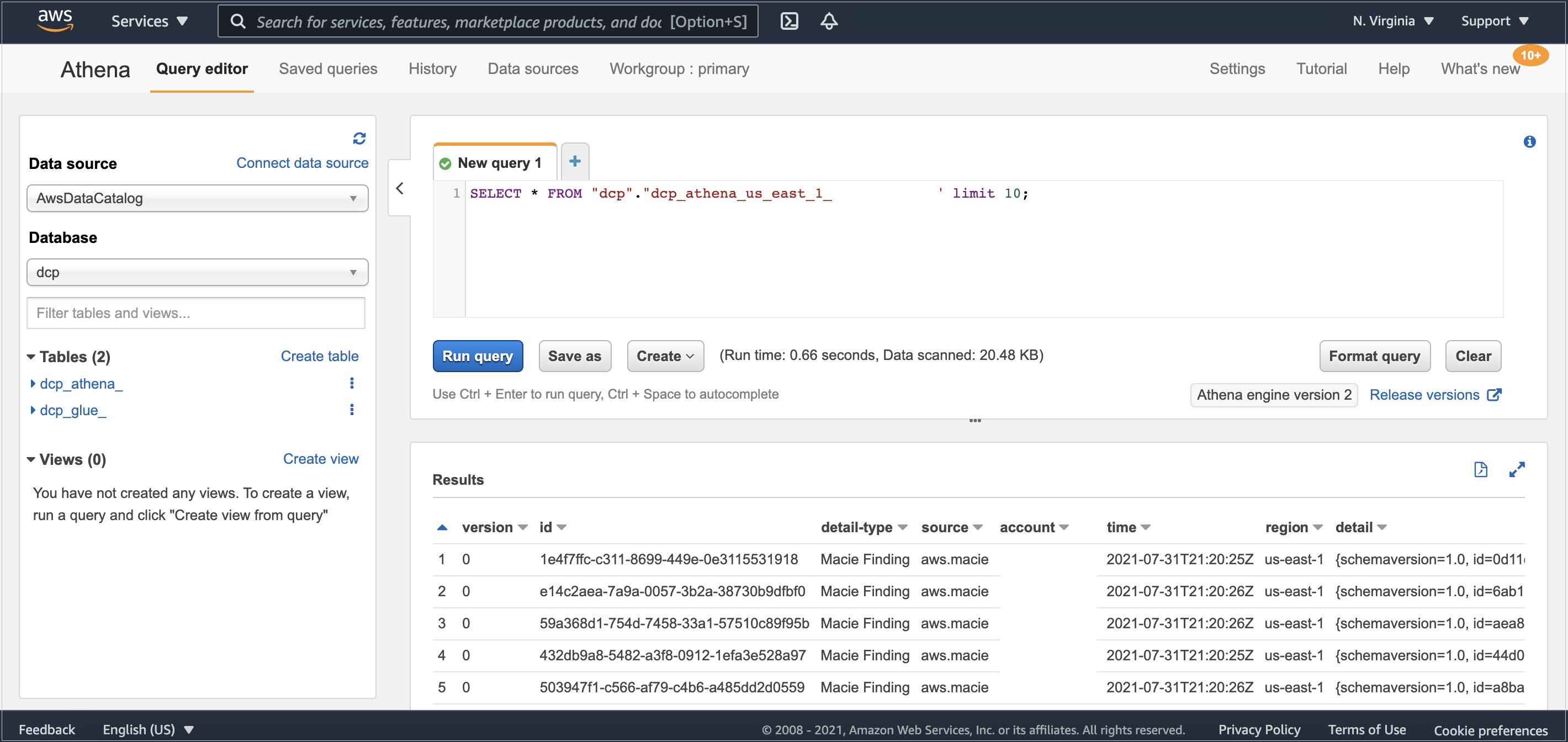
Display your data in Amazon S3 (with S3 Select)
To display your data, complete the following steps:
- On the Amazon S3 console, in the Buckets list, choose the name of the bucket that contains the output of the Salesforce data (
airflow-blog-post).
- In the Objects list, choose the name of the folder that has the object that you copied from Salesforce (
opportunity).
- Choose the raw folder and the
dt folder with the latest timestamp.
- Select any file.
- On the Actions menu, choose Query with S3 Select.
- Choose Run SQL query to preview the data.

Clean up
To avoid incurring future charges, delete the AWS CloudFormation stack and the resources that you deployed as part of this post.
- On the AWS CloudFormation console, delete the stack
MWAAirflowStack.
To clean up the deployed resources using the AWS Command Line Interface (AWS CLI), you can simply run the following command:
cdk destroy MWAAirflowStack
Make sure you are in the root path of the project when you run the command.
After confirming that you want to destroy the CloudFormation stack, the solution’s resources are deleted from your AWS account.
The following screenshot shows the process of deploying the stack:

The following screenshot confirms the stack is undeployed.

- Navigate to the Amazon S3 console and locate the two buckets containing
mwaairflowstack-mwaaenvstack and mwaairflowstack-mwaaproj that were created during the deployment.
- Select each bucket delete its contents, then delete the bucket.
- Delete the IAM role created to write on the S3 buckets.
Conclusion
ENGIE discovered significant value by using Amazon MWAA, enabling its global business units to ingest data in more productive ways. This post presented how ENGIE scaled their data ingestion pipelines using Amazon MWAA. The first part of the post described the architecture components and how to successfully deploy a CI/CD pipeline for an Amazon MWAA project template using a CodeCommit repository and plug it into CodePipeline to build, test, and package the code and custom plugins. The second part walked you through the steps to automate the ingestion process from Salesforce using Airflow with an example. For the Airflow configuration, you used Airflow variables, but you can also use Secrets Manager with Amazon MWAA using the secretsBackend parameter when deploying the stack.
The use case discussed in this post is just one example of how you can use Amazon MWAA to make it easier to set up and operate end-to-end data pipelines in the cloud at scale. For more information about Amazon MWAA, check out the User Guide.
About the Authors
 Anouar Zaaber is a Senior Engagement Manager in AWS Professional Services. He leads internal AWS, external partner, and customer teams to deliver AWS cloud services that enable the customers to realize their business outcomes.
 Amine El Mallem is a Data/ML Ops Engineer in AWS Professional Services. He works with customers to design, automate, and build solutions on AWS for their business needs.
 Armando Segnini is a Data Architect with AWS Professional Services. He spends his time building scalable big data and analytics solutions for AWS Enterprise and Strategic customers. Armando also loves to travel with his family all around the world and take pictures of the places he visits.
 Mohamed-Ali Elouaer is a DevOps Consultant with AWS Professional Services. He is part of the AWS ProServe team, helping enterprise customers solve complex problems related to automation, security, and monitoring using AWS services. In his free time, he likes to travel and watch movies.
 Julien Grinsztajn is an Architect at ENGIE. He is part of the Digital & IT Consulting ENGIE IT team working on the definition of the architecture for complex projects related to data integration and network security. In his free time, he likes to travel the oceans to meet sharks and other marine creatures.


 Lotfi Mouhib is a Senior Solutions Architect working for the Public Sector team with Amazon Web Services. He helps public sector customers across EMEA realize their ideas, build new services, and innovate for citizens. In his spare time, Lotfi enjoys cycling and running.