Tag Archives: Amazon Simple Storage Service (S3)

Automate the archive and purge data process for Amazon RDS for PostgreSQL using pg_partman, Amazon S3, and AWS Glue

Post Syndicated from Anand Komandooru original https://aws.amazon.com/blogs/big-data/automate-the-archive-and-purge-data-process-for-amazon-rds-for-postgresql-using-pg_partman-amazon-s3-and-aws-glue/

The post Archive and Purge Data for Amazon RDS for PostgreSQL and Amazon Aurora with PostgreSQL Compatibility using pg_partman and Amazon S3 proposes data archival as a critical part of data management and shows how to efficiently use PostgreSQL’s native range partition to partition current (hot) data with pg_partman and archive historical (cold) data in Amazon Simple Storage Service (Amazon S3). Customers need a cloud-native automated solution to archive historical data from their databases. Customers want the business logic to be maintained and run from outside the database to reduce the compute load on the database server. This post proposes an automated solution by using AWS Glue for automating the PostgreSQL data archiving and restoration process, thereby streamlining the entire procedure.

AWS Glue is a serverless data integration service that makes it easier to discover, prepare, move, and integrate data from multiple sources for analytics, machine learning (ML), and application development. There is no need to pre-provision, configure, or manage infrastructure. It can also automatically scale resources to meet the requirements of your data processing job, providing a high level of abstraction and convenience. AWS Glue integrates seamlessly with AWS services like Amazon S3, Amazon Relational Database Service (Amazon RDS), Amazon Redshift, Amazon DynamoDB, Amazon Kinesis Data Streams, and Amazon DocumentDB (with MongoDB compatibility) to offer a robust, cloud-native data integration solution.

The features of AWS Glue, which include a scheduler for automating tasks, code generation for ETL (extract, transform, and load) processes, notebook integration for interactive development and debugging, as well as robust security and compliance measures, make it a convenient and cost-effective solution for archival and restoration needs.

Solution overview

The solution combines PostgreSQL’s native range partitioning feature with pg_partman, the Amazon S3 export and import functions in Amazon RDS, and AWS Glue as an automation tool.

The solution involves the following steps:

  1. Provision the required AWS services and workflows using the provided AWS Cloud Development Kit (AWS CDK) project.
  2. Set up your database.
  3. Archive the older table partitions to Amazon S3 and purge them from the database with AWS Glue.
  4. Restore the archived data from Amazon S3 to the database with AWS Glue when there is a business need to reload the older table partitions.

The solution is based on AWS Glue, which takes care of archiving and restoring databases with Availability Zone redundancy. The solution is comprised of the following technical components:

  • An Amazon RDS for PostgreSQL Multi-AZ database runs in two private subnets.
  • AWS Secrets Manager stores database credentials.
  • An S3 bucket stores Python scripts and database archives.
  • An S3 Gateway endpoint allows Amazon RDS and AWS Glue to communicate privately with the Amazon S3.
  • AWS Glue uses a Secrets Manager interface endpoint to retrieve database secrets from Secrets Manager.
  • AWS Glue ETL jobs run in either private subnet. They use the S3 endpoint to retrieve Python scripts. The AWS Glue jobs read the database credentials from Secrets Manager to establish JDBC connections to the database.

You can create an AWS Cloud9 environment in one of the private subnets available in your AWS account to set up test data in Amazon RDS. The following diagram illustrates the solution architecture.

Solution Architecture

Prerequisites

For instructions to set up your environment for implementing the solution proposed in this post, refer to Deploy the application in the GitHub repo.

Provision the required AWS resources using AWS CDK

Complete the following steps to provision the necessary AWS resources:

  1. Clone the repository to a new folder on your local desktop.
  2. Create a virtual environment and install the project dependencies.
  3. Deploy the stacks to your AWS account.

The CDK project includes three stacks: vpcstack, dbstack, and gluestack, implemented in the vpc_stack.py, db_stack.py, and glue_stack.py modules, respectively.

These stacks have preconfigured dependencies to simplify the process for you. app.py declares Python modules as a set of nested stacks. It passes a reference from vpcstack to dbstack, and a reference from both vpcstack and dbstack to gluestack.

gluestack reads the following attributes from the parent stacks:

  • The S3 bucket, VPC, and subnets from vpcstack
  • The secret, security group, database endpoint, and database name from dbstack

The deployment of the three stacks creates the technical components listed earlier in this post.

Set up your database

Prepare the database using the information provided in Populate and configure the test data on GitHub.

Archive the historical table partition to Amazon S3 and purge it from the database with AWS Glue

The “Maintain and Archive” AWS Glue workflow created in the first step consists of two jobs: “Partman run maintenance” and “Archive Cold Tables.”

The “Partman run maintenance” job runs the Partman.run_maintenance_proc() procedure to create new partitions and detach old partitions based on the retention setup in the previous step for the configured table. The “Archive Cold Tables” job identifies the detached old partitions and exports the historical data to an Amazon S3 destination using aws_s3.query_export_to_s3. In the end, the job drops the archived partitions from the database, freeing up storage space. The following screenshot shows the results of running this workflow on demand from the AWS Glue console.

Archive job run result

Additionally, you can set up this AWS Glue workflow to be triggered on a schedule, on demand, or with an Amazon EventBridge event. You need to use your business requirement to select the right trigger.

Restore archived data from Amazon S3 to the database

The “Restore from S3” Glue workflow created in the first step consists of one job: “Restore from S3.”

This job initiates the run of the partman.create_partition_time procedure to create a new table partition based on your specified month. It subsequently calls aws_s3.table_import_from_s3 to restore the matched data from Amazon S3 to the newly created table partition.

To start the “Restore from S3” workflow, navigate to the workflow on the AWS Glue console and choose Run.

The following screenshot shows the “Restore from S3” workflow run details.

Restore job run result

Validate the results

The solution provided in this post automated the PostgreSQL data archival and restoration process using AWS Glue.

You can use the following steps to confirm that the historical data in the database is successfully archived after running the “Maintain and Archive” AWS Glue workflow:

  1. On the Amazon S3 console, navigate to your S3 bucket.
  2. Confirm the archived data is stored in an S3 object as shown in the following screenshot.
    Archived data in S3
  3. From a psql command line tool, use the \dt command to list the available tables and confirm the archived table ticket_purchase_hist_p2020_01 does not exist in the database.List table result after post archival

You can use the following steps to confirm that the archived data is restored to the database successfully after running the “Restore from S3” AWS Glue workflow.

  1. From a psql command line tool, use the \dt command to list the available tables and confirm the archived table ticket_history_hist_p2020_01 is restored to the database.List table results after restore

Clean up

Use the information provided in Cleanup to clean up your test environment created for testing the solution proposed in this post.

Summary

This post showed how to use AWS Glue workflows to automate the archive and restore process in RDS for PostgreSQL database table partitions using Amazon S3 as archive storage. The automation is run on demand but can be set up to be trigged on a recurring schedule. It allows you to define the sequence and dependencies of jobs, track the progress of each workflow job, view run logs, and monitor the overall health and performance of your tasks. Although we used Amazon RDS for PostgreSQL as an example, the same solution works for Amazon Aurora-PostgreSQL Compatible Edition as well. Modernize your database cron jobs using AWS Glue by using this post and the GitHub repo. Gain a high-level understanding of AWS Glue and its components by using the following hands-on workshop.


About the Authors

Anand Komandooru is a Senior Cloud Architect at AWS. He joined AWS Professional Services organization in 2021 and helps customers build cloud-native applications on AWS cloud. He has over 20 years of experience building software and his favorite Amazon leadership principle is “Leaders are right a lot.”

Li Liu is a Senior Database Specialty Architect with the Professional Services team at Amazon Web Services. She helps customers migrate traditional on-premise databases to the AWS Cloud. She specializes in database design, architecture, and performance tuning.

Neil Potter is a Senior Cloud Application Architect at AWS. He works with AWS customers to help them migrate their workloads to the AWS Cloud. He specializes in application modernization and cloud-native design and is based in New Jersey.

Vivek Shrivastava is a Principal Data Architect, Data Lake in AWS Professional Services. He is a big data enthusiast and holds 14 AWS Certifications. He is passionate about helping customers build scalable and high-performance data analytics solutions in the cloud. In his spare time, he loves reading and finds areas for home automation.

Monitor data pipelines in a serverless data lake

Post Syndicated from Virendhar Sivaraman original https://aws.amazon.com/blogs/big-data/monitor-data-pipelines-in-a-serverless-data-lake/

AWS serverless services, including but not limited to AWS Lambda, AWS Glue, AWS Fargate, Amazon EventBridge, Amazon Athena, Amazon Simple Notification Service (Amazon SNS), Amazon Simple Queue Service (Amazon SQS), and Amazon Simple Storage Service (Amazon S3), have become the building blocks for any serverless data lake, providing key mechanisms to ingest and transform data without fixed provisioning and the persistent need to patch the underlying servers. The combination of a data lake in a serverless paradigm brings significant cost and performance benefits. The advent of rapid adoption of serverless data lake architectures—with ever-growing datasets that need to be ingested from a variety of sources, followed by complex data transformation and machine learning (ML) pipelines—can present a challenge. Similarly, in a serverless paradigm, application logs in Amazon CloudWatch are sourced from a variety of participating services, and traversing the lineage across logs can also present challenges. To successfully manage a serverless data lake, you require mechanisms to perform the following actions:

  • Reinforce data accuracy with every data ingestion
  • Holistically measure and analyze ETL (extract, transform, and load) performance at the individual processing component level
  • Proactively capture log messages and notify failures as they occur in near-real time

In this post, we will walk you through a solution to efficiently track and analyze ETL jobs in a serverless data lake environment. By monitoring application logs, you can gain insights into job execution, troubleshoot issues promptly to ensure the overall health and reliability of data pipelines.

Overview of solution

The serverless monitoring solution focuses on achieving the following goals:

  • Capture state changes across all steps and tasks in the data lake
  • Measure service reliability across a data lake
  • Quickly notify operations of failures as they happen

To illustrate the solution, we create a serverless data lake with a monitoring solution. For simplicity, we create a serverless data lake with the following components:

  • Storage layer – Amazon S3 is the natural choice, in this case with the following buckets:
    • Landing – Where raw data is stored
    • Processed – Where transformed data is stored
  • Ingestion layer – For this post, we use Lambda and AWS Glue for data ingestion, with the following resources:
    • Lambda functions – Two Lambda functions that run to simulate a success state and failure state, respectively
    • AWS Glue crawlers – Two AWS Glue crawlers that run to simulate a success state and failure state, respectively
    • AWS Glue jobs – Two AWS Glue jobs that run to simulate a success state and failure state, respectively
  • Reporting layer – An Athena database to persist the tables created via the AWS Glue crawlers and AWS Glue jobs
  • Alerting layer – Slack is used to notify stakeholders

The serverless monitoring solution is devised to be loosely coupled as plug-and-play components that complement an existing data lake. The Lambda-based ETL tasks state changes are tracked using AWS Lambda Destinations. We have used an SNS topic for routing both success and failure states for the Lambda-based tasks. In the case of AWS Glue-based tasks, we have configured EventBridge rules to capture state changes. These event changes are also routed to the same SNS topic. For demonstration purposes, this post only provides state monitoring for Lambda and AWS Glue, but you can extend the solution to other AWS services.

The following figure illustrates the architecture of the solution.

The architecture contains the following components:

  • EventBridge rules – EventBridge rules that capture the state change for the ETL tasks—in this case AWS Glue tasks. This can be extended to other supported services as the data lake grows.
  • SNS topic – An SNS topic that serves to catch all state events from the data lake.
  • Lambda function – The Lambda function is the subscriber to the SNS topic. It’s responsible for analyzing the state of the task run to do the following:
    • Persist the status of the task run.
    • Notify any failures to a Slack channel.
  • Athena database – The database where the monitoring metrics are persisted for analysis.

Deploy the solution

The source code to implement this solution uses AWS Cloud Development Kit (AWS CDK) and is available on the GitHub repo monitor-serverless-datalake. This AWS CDK stack provisions required network components and the following:

  • Three S3 buckets (the bucket names are prefixed with the AWS account name and Regions, for example, the landing bucket is <aws-account-number>-<aws-region>-landing):
    • Landing
    • Processed
    • Monitor
  • Three Lambda functions:
    • datalake-monitoring-lambda
    • lambda-success
    • lambda-fail
  • Two AWS Glue crawlers:
    • glue-crawler-success
    • glue-crawler-fail
  • Two AWS Glue jobs:
    • glue-job-success
    • glue-job-fail
  • An SNS topic named datalake-monitor-sns
  • Three EventBridge rules:
    • glue-monitor-rule
    • event-rule-lambda-fail
    • event-rule-lambda-success
  • An AWS Secrets Manager secret named datalake-monitoring
  • Athena artifacts:
    • monitor database
    • monitor-table table

You can also follow the instructions in the GitHub repo to deploy the serverless monitoring solution. It takes about 10 minutes to deploy this solution.

Connect to a Slack channel

We still need a Slack channel to which the alerts are delivered. Complete the following steps:

  1. Set up a workflow automation to route messages to the Slack channel using webhooks.
  2. Note the webhook URL.

The following screenshot shows the field names to use.

The following is a sample message for the preceding template.

  1. On the Secrets Manager console, navigate to the datalake-monitoring secret.
  2. Add the webhook URL to the slack_webhook secret.

Load sample data

The next step is to load some sample data. Copy the sample data files to the landing bucket using the following command:

aws s3 cp --recursive s3://awsglue-datasets/examples/us-legislators s3://<AWS_ACCCOUNT>-<AWS_REGION>-landing/legislators

In the next sections, we show how Lambda functions, AWS Glue crawlers, and AWS Glue jobs work for data ingestion.

Test the Lambda functions

On the EventBridge console, enable the rules that trigger the lambda-success and lambda-fail functions every 5 minutes:

  • event-rule-lambda-fail
  • event-rule-lambda-success

After a few minutes, the failure events are relayed to the Slack channel. The following screenshot shows an example message.

Disable the rules after testing to avoid repeated messages.

Test the AWS Glue crawlers

On the AWS Glue console, navigate to the Crawlers page. Here you can start the following crawlers:

  • glue-crawler-success
  • glue-crawler-fail

In a minute, the glue-crawler-fail crawler’s status changes to Failed, which triggers a notification in Slack in near-real time.

Test the AWS Glue jobs

On the AWS Glue console, navigate to the Jobs page, where you can start the following jobs:

  • glue-job-success
  • glue-job-fail

In a few minutes, the glue-job-fail job status changes to Failed, which triggers a notification in Slack in near-real time.

Analyze the monitoring data

The monitoring metrics are persisted in Amazon S3 for analysis and can be used of historical analysis.

On the Athena console, navigate to the monitor database and run the following query to find the service that failed the most often:

SELECT service_type, count(*) as "fail_count"
FROM "monitor"."monitor"
WHERE event_type = 'failed'
group by service_type
order by fail_count desc;

Over time with rich observability data – time series based monitoring data analysis will yield interesting findings.

Clean up

The overall cost of the solution is less than one dollar but to avoid future costs, make sure to clean up the resources created as part of this post.

Summary

The post provided an overview of a serverless data lake monitoring solution that you can configure and deploy to integrate with enterprise serverless data lakes in just a few hours. With this solution, you can monitor a serverless data lake, send alerts in near-real time, and analyze performance metrics for all ETL tasks operating in the data lake. The design was intentionally kept simple to demonstrate the idea; you can further extend this solution with Athena and Amazon QuickSight to generate custom visuals and reporting. Check out the GitHub repo for a sample solution and further customize it for your monitoring needs.


About the Authors

Virendhar (Viru) Sivaraman is a strategic Senior Big Data & Analytics Architect with Amazon Web Services. He is passionate about building scalable big data and analytics solutions in the cloud. Besides work, he enjoys spending time with family, hiking & mountain biking.

Vivek Shrivastava is a Principal Data Architect, Data Lake in AWS Professional Services. He is a Bigdata enthusiast and holds 14 AWS Certifications. He is passionate about helping customers build scalable and high-performance data analytics solutions in the cloud. In his spare time, he loves reading and finds areas for home automation.

Welcome to AWS Storage Day 2023

Post Syndicated from Veliswa Boya original https://aws.amazon.com/blogs/aws/welcome-to-aws-storage-day-2023/

Welcome to the fifth annual AWS Storage Day! This virtual event is happening today starting at 9:00 AM Pacific Time (12:00 PM Eastern Time) and is available for you to watch on the AWS On Air Twitch channel. The first AWS Storage Day was hosted in 2019, and this event has grown into an innovation day that we look forward to delivering to you every year. In last year’s Storage Day post, I wrote about the constant innovations in AWS Storage aimed at helping you put your data to work while keeping it secure and protected. This year, Storage Day is focused on storage for AI/ML, data protection and resiliency, and the benefits of moving to the cloud.

AWS Storage Day Key Themes
When it comes to storage for AI/ML, data volumes are increasing at an unprecedented rate, exploding from terabytes to petabytes and even to exabytes. With a modern data architecture on AWS, you can rapidly build scalable data lakes, use a broad and deep collection of purpose-built data services, scale your systems at a low cost without compromising performance, share data across organizational boundaries, and manage compliance, security, and governance, allowing you to make decisions with speed and agility at scale.
To train machine learning models and build Generative AI applications, you must have the right data strategy in place. So, I’m happy to see that, among the list of sessions to look forward to at the live event, the Optimize generative AI and ML with AWS Infrastructure session will discuss how you can transform your data into meaningful insights.

Whether you’re just getting started with the cloud, planning to migrate applications to AWS, or already building applications on AWS, we have resources to help you protect your data and meet your business continuity objectives. Our data protection and resiliency features and solutions can help you meet your business continuity goals and deliver disaster recovery during data loss events, across recovery point and time objectives (RPO and RTO). With the unprecedented data growth happening in the world today, determining where your data is stored, how it’s secured, and who has access to it is a higher priority than ever. Be sure to join the Protect data in AWS amid a rapidly evolving cyber landscape session to learn more.

When moving data to the cloud, you need to understand where you’re moving it for different use cases, the types of data you’re moving, and the network resources available, among other considerations. There are many reasons to move to the cloud, recently, Enterprise Strategy Group (ESG) validated that organizations reduced compute, networking, and storage costs by up to 66 percent by migrating on-premises workloads to AWS Cloud infrastructure. ESG confirmed that migrating on-premises workloads to AWS provides organizations with reduced costs, increased performance, improved operational efficiency, faster time to value, and improved business agility.
We have a number of sessions that discuss how to move to the cloud, based on your use case. I’m most looking forward to the Hybrid cloud storage and edge compute: AWS, where you need it session, which will discuss considerations for workloads that can’t fully move to the cloud.

Tune in to learn from experts about new announcements, leadership insights, and educational content related to the broad portfolio of AWS Storage services and features that address all these themes and more. Today, we have announcements related to Amazon Simple Storage Service (Amazon S3), Amazon FSx for Windows File Server, Amazon Elastic File System (Amazon EFS), Amazon FSx for OpenZFS, and more.

Let’s get into it.

15 Years of Amazon EBS
Not long ago, I was reading Jeff Barr’s post titled 15 Years of AWS Blogging! In this post, Jeff mentioned a few posts he wrote for the earliest AWS services and features. Amazon Elastic Block Store (Amazon EBS) is on this list as a service that simplifies the use of Amazon EC2.

Well, it’s been 15 years since the launch of Amazon EBS was announced, and today we celebrate 15 years of this service. If you were one of the original users who put Amazon EBS to good use and provided us with the very helpful feedback that helped us invent and simplify, iterate and improve, I’m sure you can’t believe how time flies. Today, Amazon EBS handles more than 100 trillion I/O operations daily, and over 390 million EBS volumes are created every day.

If you’re new to Amazon EBS, join us for a fireside chat with Matt Garman, Senior Vice President, Sales, Marketing, and Global Services at AWS, and learn the strategy and customer challenges behind the launch of the service in 2008. You’ll also hear from long-term EBS customer, Stripe, about its growth with EBS since Stripe was launched 12 years ago.

Amazon EBS has continuously improved its scalability and performance to support more customer workloads as the direct storage attachment for Amazon EC2 instances. With the launch of Amazon EC2 M7i instances, powered by custom 4th Generation Intel Xeon Scalable processors, on August 2, you can attach up to 128 Amazon EBS volumes, an increase from 28 on a previous generation M6i instance. The higher number of volume attachments means you can increase storage density per instance and improve resource utilization, reducing total compute cost.

You can host up to 127 containers per instance for larger database applications and scale them more cost effectively before needing to provision more instances and only pay for resources you need. With a higher number of volume attachments, you can fully utilize the memory and vCPU available on these powerful M7i instances as your database storage footprint grows. EBS is also increasing the number of multi-volume snapshots you can create, for up to 128 EBS volumes attached to an instance, enabling you to create crash-consistent backups of all volumes attached to an instance.

Join the 15 years of innovations with Amazon EBS session for a discussion about how the original vision for Amazon EBS has evolved to meet your growing demands for cloud infrastructure.

Mountpoint for Amazon S3
Now generally available, Mountpoint for Amazon S3 is a new open source file client that delivers high throughput access, lowering compute costs for data lakes on Amazon S3. Mountpoint for Amazon S3 is a file client that translates local file system API calls to S3 object API calls. Using Mountpoint for Amazon S3, you can mount an Amazon S3 bucket as a local file system on your compute instance, to access your objects through a file interface with the elastic storage and throughput of Amazon S3. Mountpoint for Amazon S3 supports sequential and random read operations on existing files, and sequential write operations for creating new files.

The Deep dive and demo of Mountpoint for Amazon S3 session demonstrates how to use the file client to access objects in Amazon S3 using file APIs, making it easier to store data at scale and maximize the value of your data with analytics and machine learning workloads. Read this blog post to learn more about Mountpoint for Amazon S3 and how to get started, including a demo.

Put Cold Storage to Work Faster with Amazon S3 Glacier Flexible Retrieval
Amazon S3 Glacier Flexible Retrieval improves data restore time by up to 85 percent, at no additional cost. Faster data restores automatically apply to the Standard retrieval tier when using Amazon S3 Batch Operations. These restores begin to return objects within minutes, so you can process restored data faster. Processing restored data in parallel with ongoing restores helps you accelerate data workflows and quickly respond to business needs. Now, whether you’re transcoding media, restoring operational backups, training machine learning models, or analyzing historical data, you can speed up your data restores from archive.

Coupled with the S3 Glacier improvements to restore throughput by up to 10 times for millions of objects announced in 2022, S3 Glacier data restores of all sizes now benefit from both faster starts and shorter completion times.

Join the Maximize the value of cold data with Amazon S3 Glacier session to learn how Amazon S3 Glacier is helping organizations of all sizes and from all industries transform their data archiving to unlock business value, increase agility, and save on storage costs. Read this blog post to learn more about the Amazon S3 Glacier Flexible Retrieval performance improvements and follow step-by-step guidance on how to get started with faster standard retrievals from S3 Glacier Flexible Retrieval.

Supporting a Broad Spectrum of File Workloads
To serve a broad spectrum of use cases that rely on file systems, we offer a portfolio of file system services, each targeting a different set of needs. Amazon EFS is a serverless file system built to deliver an elastic experience for sharing data across compute resources. Amazon FSx makes it easier and cost-effective for you to launch, run, and scale feature-rich, high-performance file systems in the cloud, enabling you to move to the cloud with no changes to your code, processes, or how you manage your data.

Power ML research and big data analytics with Amazon EFS
Amazon EFS offers serverless and fully scalable file storage, designed for high scalability in both storage capacity and throughput performance. Just last week, we announced enhanced support for faster read and write IOPS, making it easier to power more demanding workloads. We’ve improved the performance capabilities of Amazon EFS by adding support for up to 55,000 read IOPS and up to 25,000 write IOPS per file system. These performance enhancements help you to run more demanding workflows, such as machine learning (ML) research with KubeFlow, financial simulations with IBM Symphony, and big data processing with Domino Data Lab, Hadoop, and Spark.

Join the Build and run analytics and SaaS applications at scale session to hear how recent Amazon EFS performance improvements can help power more workloads.

Multi-AZ file systems on Amazon FSx for OpenZFS
You can now use a multi-AZ deployment option when creating file systems on Amazon FSx for OpenZFS, making it easier to deploy file storage that spans multiple AWS Availability Zones to provide multi-AZ resilience for business-critical workloads. With this launch, you can take advantage of the power, agility, and simplicity of Amazon FSx for OpenZFS for a broader set of workloads, including business-critical workloads like database, line-of-business, and web-serving applications that require highly available shared storage that spans multiple AZs.

The new multi-AZ file systems are designed to deliver high levels of performance to serve a broad variety of workloads, including performance-intensive workloads such as financial services analytics, media and entertainment workflows, semiconductor chip design, and game development and streaming, up to 21 GB per second of throughput and over 1 million IOPS for frequently accessed cached data, and up to 10 GB per second and 350,000 IOPS for data accessed from persistent disk storage.

Join the Migrate NAS to AWS to reduce TCO and gain agility session to learn more about multi-AZs with Amazon FSx for OpenZFS.

New, Higher Throughput Capacity Levels on Amazon FSx for Windows File Server
Performance improvements for Amazon FSx for Windows File Server help you accelerate time-to-results for performance-intensive workloads such as SQL Server databases, media processing, cloud video editing, and virtual desktop infrastructure (VDI).

We’re adding four new, higher throughput capacity levels to increase the maximum I/O available up to 12 GB per second from the previous I/O of 2 GB per second. These throughput improvements come with correspondingly higher levels of disk IOPS, designed to deliver an increase up to 350,000 IOPS.

In addition, by using FSx for Windows File Server, you can provision IOPS higher than the default 3 IOPS per GiB for your SSD file system. This allows you to scale SSD IOPS independently from storage capacity, allowing you to optimize costs for performance-sensitive workloads.

Join the Migrate NAS to AWS to reduce TCO and gain agility session to learn more about the performance improvements for Amazon FSx for Windows File Server.

Logically Air-Gapped Vault for AWS Backup
AWS Backup is a fully managed, policy-based data protection solution that enables customers to centralize and automate backup restores across 19 AWS services (spanning compute, storage, and databases) and third-party applications such as VMware Cloud on AWS and on-premises, as well as SAP HANA on Amazon EC2.

Today, we’re announcing the preview of logically air-gapped vault as a new type of AWS Backup Vault that acts as an additional layer of protection to mitigate against malware events. With logically air-gapped vault, customers can recover their application data through a different trusted account.

Join the Deep dive on data recovery for ransomware events session to learn more about logically air-gapped vault for AWS Backup.

Copy Data to and from Other Clouds with AWS DataSync
AWS DataSync is an online data movement and discovery service that simplifies data migration and helps you quickly, easily, and securely transfer your file or object data to, from, and between AWS storage services. In addition to support of data migration to and from AWS storage services, DataSync supports copying to and from other clouds such as Google Cloud Storage, Azure Files, and Azure Blob Storage. Using DataSync, you can move your object data at scale between Amazon S3 compatible storage on other clouds and AWS storage services such as Amazon S3. We’re now expanding the support of DataSync for copying data to and from other clouds to include DigitalOcean Spaces, Wasabi Cloud Storage, Backblaze B2 Cloud Storage, Cloudflare R2 Storage, and Oracle Cloud Storage.

Join the Identify and accelerate data migrations at scale session to learn more about this expanded support for DataSync.

Join Us Online
Join us today for the AWS Storage Day virtual event on the AWS On Air channel on Twitch. The event will be live starting at 9:00 AM Pacific Time (12:00 PM Eastern Time) on August 9. All sessions will be available on demand approximately two days after Storage Day.

We look forward to seeing you on Twitch!

– Veliswa 

Mountpoint for Amazon S3 – Generally Available and Ready for Production Workloads

Post Syndicated from Jeff Barr original https://aws.amazon.com/blogs/aws/mountpoint-for-amazon-s3-generally-available-and-ready-for-production-workloads/

Mountpoint for Amazon S3 is an open source file client that makes it easy for your file-aware Linux applications to connect directly to Amazon Simple Storage Service (Amazon S3) buckets. Announced earlier this year as an alpha release, it is now generally available and ready for production use on your large-scale read-heavy applications: data lakes, machine learning training, image rendering, autonomous vehicle simulation, ETL, and more. It supports file-based workloads that perform sequential and random reads, sequential (append only) writes, and that don’t need full POSIX semantics.

Why Files?
Many AWS customers use the S3 APIs and the AWS SDKs to build applications that can list, access, and process the contents of an S3 bucket. However, many customers have existing applications, commands, tools, and workflows that know how to access files in UNIX style: reading directories, opening & reading existing files, and creating & writing new ones. These customers have asked us for an official, enterprise-ready client that supports performant access to S3 at scale. After speaking with these customers and asking lots of questions, we learned that performance and stability were their primary concerns, and that POSIX compliance was not a necessity.

When I first wrote about Amazon S3 back in 2006 I was very clear that it was intended to be used as an object store, not as a file system. While you would not want use the Mountpoint / S3 combo to store your Git repositories or the like, using it in conjunction with tools that can read and write files, while taking advantage of S3’s scale and durability, makes sense in many situations.

All About Mountpoint
Mountpoint is conceptually very simple. You create a mount point and mount an Amazon S3 bucket (or a path within a bucket) at the mount point, and then access the bucket using shell commands (ls, cat, dd, find, and so forth), library functions (open, close, read, write, creat, opendir, and so forth) or equivalent commands and functions as supported in the tools and languages that you already use.

Under the covers, the Linux Virtual Filesystem (VFS) translates these operations into calls to Mountpoint, which in turns translates them into calls to S3: LIST, GET, PUT, and so forth. Mountpoint strives to make good use of network bandwidth, increasing throughput and allowing you to reduce your compute costs by getting more work done in less time.

Mountpoint can be used from an Amazon Elastic Compute Cloud (Amazon EC2) instance, or within an Amazon Elastic Container Service (Amazon ECS) or Amazon Elastic Kubernetes Service (EKS) container. It can also be installed on your existing on-premises systems, with access to S3 either directly or over an AWS Direct Connect connection via AWS PrivateLink for Amazon S3.

Installing and Using Mountpoint for Amazon S3
Mountpoint is available in RPM format and can easily be installed on an EC2 instance running Amazon Linux. I simply fetch the RPM and install it using yum:

$ wget https://s3.amazonaws.com/mountpoint-s3-release/latest/x86_64/mount-s3.rpm
$ sudo yum install ./mount-s3.rpm

For the last couple of years I have been regularly fetching images from several of the Washington State Ferry webcams and storing them in my wsdot-ferry bucket:

I collect these images in order to track the comings and goings of the ferries, with a goal of analyzing them at some point to find the best times to ride. My goal today is to create a movie that combines an entire day’s worth of images into a nice time lapse. I start by creating a mount point and mounting the bucket:

$ mkdir wsdot-ferry
$  mount-s3 wsdot-ferry wsdot-ferry

I can traverse the mount point and inspect the bucket:

$ cd wsdot-ferry
$ ls -l | head -10
total 0
drwxr-xr-x 2 jeff jeff 0 Aug  7 23:07 2020_12_30
drwxr-xr-x 2 jeff jeff 0 Aug  7 23:07 2020_12_31
drwxr-xr-x 2 jeff jeff 0 Aug  7 23:07 2021_01_01
drwxr-xr-x 2 jeff jeff 0 Aug  7 23:07 2021_01_02
drwxr-xr-x 2 jeff jeff 0 Aug  7 23:07 2021_01_03
drwxr-xr-x 2 jeff jeff 0 Aug  7 23:07 2021_01_04
drwxr-xr-x 2 jeff jeff 0 Aug  7 23:07 2021_01_05
drwxr-xr-x 2 jeff jeff 0 Aug  7 23:07 2021_01_06
drwxr-xr-x 2 jeff jeff 0 Aug  7 23:07 2021_01_07
$
$  cd 2020_12_30
$ ls -l
total 0
drwxr-xr-x 2 jeff jeff 0 Aug  7 23:07 fauntleroy_holding
drwxr-xr-x 2 jeff jeff 0 Aug  7 23:07 fauntleroy_way
drwxr-xr-x 2 jeff jeff 0 Aug  7 23:07 lincoln
drwxr-xr-x 2 jeff jeff 0 Aug  7 23:07 trenton
drwxr-xr-x 2 jeff jeff 0 Aug  7 23:07 vashon_112_north
drwxr-xr-x 2 jeff jeff 0 Aug  7 23:07 vashon_112_south
drwxr-xr-x 2 jeff jeff 0 Aug  7 23:07 vashon_bunker_north
drwxr-xr-x 2 jeff jeff 0 Aug  7 23:07 vashon_bunker_south
drwxr-xr-x 2 jeff jeff 0 Aug  7 23:07 vashon_holding
$
$ cd fauntleroy_holding
$  ls -l | head -10
total 2680
-rw-r--r-- 1 jeff jeff  19337 Feb 10  2021 17-12-01.jpg
-rw-r--r-- 1 jeff jeff  19380 Feb 10  2021 17-15-01.jpg
-rw-r--r-- 1 jeff jeff  19080 Feb 10  2021 17-18-01.jpg
-rw-r--r-- 1 jeff jeff  17700 Feb 10  2021 17-21-01.jpg
-rw-r--r-- 1 jeff jeff  17016 Feb 10  2021 17-24-01.jpg
-rw-r--r-- 1 jeff jeff  16638 Feb 10  2021 17-27-01.jpg
-rw-r--r-- 1 jeff jeff  16713 Feb 10  2021 17-30-01.jpg
-rw-r--r-- 1 jeff jeff  16647 Feb 10  2021 17-33-02.jpg
-rw-r--r-- 1 jeff jeff  16750 Feb 10  2021 17-36-01.jpg
$

I can create my animation with a single command:

$ ffmpeg -framerate 10 -pattern_type glob -i "*.jpg" ferry.gif

And here’s what I get:

As you can see, I used Mountpoint to access the existing image files and to write the newly created animation back to S3. While this is a fairly simple demo, it does show how you can use your existing tools and skills to process objects in an S3 bucket. Given that I have collected several million images over the years, being able to process them without explicitly syncing them to my local file system is a big win.

Mountpoint for Amazon S3 Facts
Here are a couple of things to keep in mind when using Mountpoint:

Pricing – There are no new charges for the use of Mountpoint; you pay only for the underlying S3 operations. You can also use Mountpoint to access requester-pays buckets.

PerformanceMountpoint is able to take advantage of the elastic throughput offered by S3, including data transfer at up to 100 Gb/second between each EC2 instance and S3.

CredentialsMountpoint accesses your S3 buckets using the AWS credentials that are in effect when you mount the bucket. See the CONFIGURATION doc for more information on credentials, bucket configuration, use of requester pays, some tips for the use of S3 Object Lambda, and more.

Operations & SemanticsMountpoint supports basic file operations, and can read files up to 5 TB in size. It can list and read existing files, and it can create new ones. It cannot modify existing files or delete directories, and it does not support symbolic links or file locking (if you need POSIX semantics, take a look at Amazon FSx for Lustre). For more information about the supported operations and their interpretation, read the SEMANTICS document.

Storage Classes – You can use Mountpoint to access S3 objects in all storage classes except S3 Glacier Flexible Retrieval, S3 Glacier Deep Archive, S3 Intelligent-Tiering Archive Access Tier, and S3 Intelligent-Tiering Deep Archive Access Tier.

Open SourceMountpoint is open source and has a public roadmap. Your contributions are welcome; be sure to read our Contributing Guidelines and our Code of Conduct first.

Hop On
As you can see, Mountpoint is really cool and I am guessing that you are going to find some awesome ways to put it to use in your applications. Check it out and let me know what you think!

Jeff;

New – Improve Amazon S3 Glacier Flexible Restore Time By Up To 85% Using Standard Retrieval Tier and S3 Batch Operations

Post Syndicated from Channy Yun original https://aws.amazon.com/blogs/aws/new-improve-amazon-s3-glacier-flexible-restore-time-by-up-to-85-using-standard-retrieval-tier-and-s3-batch-operations/

Last year, Amazon S3 Glacier celebrated its tenth anniversary. Amazon S3 Glacier is the leader in cloud cold storage, and I wrote about its innovations over the last decade.

The Amazon S3 Glacier storage classes provide you with long-term, secure, and durable storage options to optimally archive your data at the lowest cost. The Amazon S3 Glacier storage classes (Amazon S3 Glacier Instant Retrieval, Amazon S3 Glacier Flexible Retrieval, and Amazon S3 Glacier Deep Archive) are purpose-built for colder data, providing you with retrieval flexibility from milliseconds to days, in addition to the ability to store archive data for as low as $1 per terabyte per month.

Many customers tell us that they are keeping their data for longer periods of time because they recognize its future value potential, and that they are already monetizing subsets of their archival data, or plan to use large sets of their archive data in the future. Modern data archiving is not only about optimizing storage costs for cold data; it’s also about setting up mechanisms so that when you need to put that data to work for your business, you can access it as quickly as your business requirements demand.

In 2022, AWS customers restored over 32 billion objects from Amazon S3 Glacier. Customers need to retrieve archived objects quickly when transcoding media, restoring operational backups, training machine learning (ML) models, or analyzing historical data. While customers using S3 Glacier Instant Retrieval can access their data in just milliseconds, S3 Glacier Flexible Retrieval is lower cost and provides three retrieval options: expedited retrievals in 1–5 minutes, standard retrievals in 3–5 hours, and free bulk retrievals in 5–12 hours. S3 Glacier Deep Archive is our lowest cost storage class and provides data retrieval within 12 hours using the standard retrieval option or 48 hours using the bulk retrieval option.

In November 2022, Amazon S3 Glacier improved restore throughput by up to 10 times at no additional cost when retrieving large volumes of archived data in S3 Glacier Flexible Retrieval and S3 Glacier Deep Archive. With Amazon S3 Batch Operations, you can automatically initiate requests at a faster rate, allowing you to restore billions of objects containing petabytes of data.

To continue the decade-long trend of cold storage innovation, we are announcing today the general availability of faster Standard retrievals from S3 Glacier Flexible Retrieval by up to 85 percent, at no additional cost. Faster data restores automatically apply to the Standard retrieval tier when using S3 Batch Operations.

Using S3 Batch Operations, you can restore archived data at scale by providing a manifest of objects to be retrieved and specifying a retrieval tier. With S3 Batch Operations, restores in the Standard retrieval tier now typically begin to return objects to you within minutes, down from 3–5 hours, so you can easily speed up your data restores from archive.

Additionally, S3 Batch Operations improves overall restore throughput by applying new performance optimizations to your jobs. As a result, you can restore your data faster and process restored objects sooner. Processing restored data in parallel with ongoing restores helps you accelerate data workflows and quickly respond to business needs.

Getting Started with Faster Standard Retrievals from S3 Glacier Flexible Retrieval
To restore archived data with this performance improvement, you can use S3 Batch Operations to perform both large- and small-scale batch operations on S3 objects. S3 Batch Operations can perform a single operation on lists of S3 objects that you specify. You can use S3 Batch Operations through the AWS Management Console, AWS Command Line Interface (AWS CLI), SDKs, or REST API.

To create a batch job, choose Batch Operations on the left navigation pane of the Amazon S3 console and choose Create job. You can select one of the manifest formats, a list of S3 objects that contains object keys that you want to retrieve. If your manifest format is a CSV file, each row in the file must include the bucket name, object key, and, optionally, the object version.

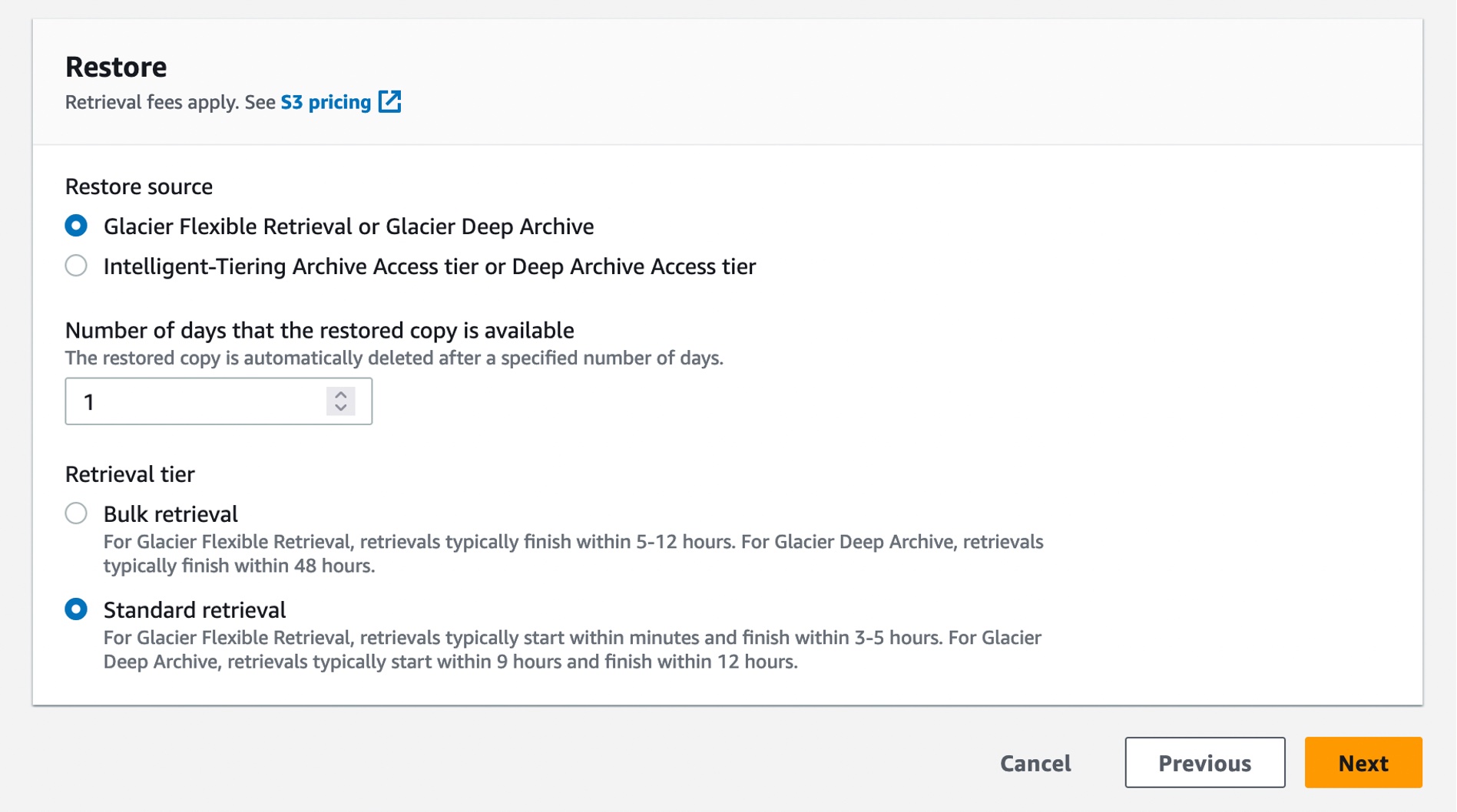
In the next step, choose the operation that you want to perform on all objects listed in the manifest. The Restore operation initiates restore requests for archived objects on a list of S3 objects that you specify. Using a restore operation results in a restore request for every object that is specified in the manifest.

When you restore with the Standard retrieval tier from the S3 Glacier Flexible Retrieval storage class, you automatically get faster retrievals.

You can also create a restore job with S3InitiateRestoreObject job using the AWS CLI:

$aws s3control create-job \
     --region us-east-1 \
     --account-id 123456789012 \
     --operation '{"S3InitiateRestoreObject": { "ExpirationInDays": 1, "GlacierJobTier":"STANDARD"} }' \
     --report '{"Bucket":"arn:aws:s3:::reports-bucket ","Prefix":"batch-op-restore-job", "Format":" S3BatchOperations_CSV_20180820","Enabled":true,"ReportScope":"FailedTasksOnly"}' \
     --manifest '{"Spec":{"Format":"S3BatchOperations_CSV_20180820", "Fields":["Bucket","Key"]},"Location":{"ObjectArn":"arn:aws:s3:::inventory-bucket/inventory_for_restore.csv", "ETag":"<ETag>"}}' \
     --role-arn arn:aws:iam::123456789012:role/s3batch-role

You can then check the status of the job submission of the requests by running the following CLI command:

$ aws s3control describe-job \
     --region us-east-1 \
     --account-id 123456789012 \
     --job-id <JobID> \
     --query 'Job'.'ProgressSummary'

You can view and update the job status, add notifications and logging, track job failures, and generate completion reports. S3 Batch Operations job activity is recorded as events in AWS CloudTrail. For tracking job events, you can create a custom rule in Amazon EventBridge and send these events to the target notification resource of your choice, such as Amazon Simple Notification Service (Amazon SNS).

When you create an S3 Batch Operations job, you can also request a completion report for all tasks or just for failed tasks. The completion report contains additional information for each task, including the object key name and version, status, error codes, and descriptions of any errors.

For more information, see Tracking job status and completion reports in the Amazon S3 User Guide.

Here is the result of a sample retrieval job with 250 objects, each sized 100 MB. As you can see from the Previous restore performance line (blue line at the right), these restores would typically finish in 3–5 hours using Standard retrievals. Now, when you use Standard retrievals with S3 Batch Operations, your job typically starts within minutes, as shown in the Improved restore performance line (orange line at the left), improving data restore time by up to 85 percent.

To learn more, see Restoring archived objects at scale from the Amazon S3 Glacier storage classes on the AWS Storage Blog and Restoring an archived object in the Amazon S3 User Guide.

Now Available
Faster standard retrievals for Amazon S3 Glacier Flexible Retrieval are now available in all AWS Regions, including the AWS GovCloud (US) Regions and China Regions. This performance improvement is available to you at no additional cost. You are charged for S3 Batch Operations and data retrievals. For more information, see the S3 pricing page.

Lastly, we published a new ebook titled “Maximize the value of cold storage with Amazon S3 Glacier“. Read this ebook to learn how Amazon S3 Glacier is helping organizations of all sizes and from all industries transform their data archiving to unlock business value, increase agility, and save on storage costs.

To learn more, visit the S3 Glacier storage classes page and getting started guide, and send feedback to AWS re:Post for S3 Glacier or through your usual AWS Support contacts.

I’m really excited for you to start using this new feature, and I look forward to hearing about even more ways you are reinventing your business with archive data.

Channy

Improving medical imaging workflows with AWS HealthImaging and SageMaker

Post Syndicated from Sukhomoy Basak original https://aws.amazon.com/blogs/architecture/improving-medical-imaging-workflows-with-aws-healthimaging-and-sagemaker/

Medical imaging plays a critical role in patient diagnosis and treatment planning in healthcare. However, healthcare providers face several challenges when it comes to managing, storing, and analyzing medical images. The process can be time-consuming, error-prone, and costly.

There’s also a radiologist shortage across regions and healthcare systems, making the demand for this specialty increases due to an aging population, advances in imaging technology, and the growing importance of diagnostic imaging in healthcare.

As the demand for imaging studies continues to rise, the limited number of available radiologists results in delays in available appointments and timely diagnoses. And while technology enables healthcare delivery improvements for clinicians and patients, hospitals seek additional tools to solve their most pressing challenges, including:

  • Professional burnout due to an increasing demand for imaging and diagnostic services
  • Labor-intensive tasks, such as volume measurement or structural segmentation of images
  • Increasing expectations from patients expecting high-quality healthcare experiences that match retail and technology in terms of convenience, ease, and personalization

To improve clinician and patient experiences, run your picture archiving and communication system (PACS) with an artificial intelligence (AI)-enabled diagnostic imaging cloud solution to securely gain critical insights and improve access to care.

AI helps reduce the radiologist burndown rate through automation. For example, AI saves radiologist chest x-ray interpretation time. It is also a powerful tool to identify areas that need closer inspection, and helps capture secondary findings that weren’t initially identified. The advancement of interoperability and analytics gives radiologist a 360-degree, longitudinal view of patient health records to provide better healthcare at potentially lower costs.

AWS offers services to address these challenges. This blog post discusses AWS HealthImaging (AWS AHI) and Amazon SageMaker, and how they are used together to improve healthcare providers’ medical imaging workflows. This ultimately accelerates imaging diagnostics and increases radiology productivity. AWS AHI enables developers to deliver performance, security, and scale to cloud-native medical imaging applications. It allows ingestion of Digital Imaging and Communication in Medicine (DICOM) images. Amazon SageMaker provides end-to-end solution for AI and machine learning.

Let’s explore an example use case involving X-rays after an auto accident. In this diagnostic medical imaging workflow, a patient is in the emergency room. From there:

  • The patient undergoes an X-ray to check for fractures.
  • The scanned acquisition device images flow to the PACS system.
  • The radiologist reviews the information gathered from this procedure and authors the report.
  • The patient workflow continues as the reports are made available to the referring physician.

Next-generation imaging solutions and workflows

Healthcare providers can use AWS AHI and Amazon SageMaker together to enable next-generation imaging solutions and improve medical imaging workflows. The following architecture illustrates this example.

X-ray images are sent to AWS HealthImaging and an Amazon SageMaker endpoint extracts insights.

Figure 1: X-ray images are sent to AWS HealthImaging and an Amazon SageMaker endpoint extracts insights.

Let’s review the architecture and the key components:

1. Imaging Scanner: Captures the images from a patient’s body. Depending on the modality, this can be an X-ray detector; a series of detectors in a CT scanner; a magnetic field and radio frequency coils in an MRI scanner; or an ultrasound transducer. This example uses an X-ray device.

2. Amazon SQS message queue: Consumes event from S3 bucket and triggers an AWS Step Functions workflow orchestration.

3. AWS Step Functions runs the transform and import jobs to further process and import the images into AWS AHI data store instance.

4. The final diagnostic image—along with any relevant patient information and metadata—is stored in the AWS AHI datastore. This allows for efficient imaging date retrieval and management. It also enables medical imaging data access with sub-second image retrieval latencies at scale, powered by cloud-native APIs and applications from AWS partners.

5. Radiologists responsible for ground truth for ML images perform medical image annotations using Amazon SageMaker Ground Truth. They visualize and label DICOM images using a custom data labeling workflow—a fully managed data labeling service that supports built-in or custom data labeling workflows. They also leverage tools like 3D Slicer for interactive medical image annotations.

6. Data scientists build or leverage built-in deep learning models using the annotated images on Amazon SageMaker. SageMaker offers a range of deployment options that vary from low latency and high throughput to long-running inference jobs. These options include considerations for batch, real-time, or near real-time inference.

7. Healthcare providers use AWS AHI and Amazon SageMaker to run AI-assisted detection and interpretation workflow. This workflow is used to identify hard-to-see fractures, dislocations, or soft tissue injuries to allow surgeons and radiologist to be more confident in their treatment choices.

8. Finally, the image stored in AWS AHI is displayed on a monitor or other visual output device where it can be analyzed and interpreted by a radiologist or other medical professional.

  • The Open Health Imaging Foundation (OHIF) Viewer is an open source, web-based, medical imaging platform. It provides a core framework for building complex imaging applications.
  • Radical Imaging or Arterys are AWS partners that provide OHIF-based medical imaging viewer.

Each of these components plays a critical role in the overall performance and accuracy of the medical imaging system as well as ongoing research and development focused on improving diagnostic outcomes and patient care. AWS AHI uses efficient metadata encoding, lossless compression, and progressive resolution data access to provide industry leading performance for loading images. Efficient metadata encoding enables image viewers and AI algorithms to understand the contents of a DICOM study without having to load the image data.

Security

The AWS shared responsibility model applies to data protection in AWS AHI and Amazon SageMaker.

Amazon SageMaker is HIPAA-eligible and can operate with data containing Protected Health Information (PHI). Encryption of data in transit is provided by SSL/TLS and is used when communicating both with the front-end interface of Amazon SageMaker (to the Notebook) and whenever Amazon SageMaker interacts with any other AWS services.

AWS AHI is also HIPAA-eligible service and provides access control at the metadata level, ensuring that each user and application can only see the images and metadata fields that are required based upon their role. This prevents the proliferation of Patient PHI. All access to AWS AHI APIs is logged in detail in AWS CloudTrail.

Both of these services leverage AWS Key Management service (AWS KMS) to satisfy the requirement that PHI data is encrypted at rest.

Conclusion

In this post, we reviewed a common use case for early detection and treatment of conditions, resulting in better patient outcomes. We also covered an architecture that can transform the radiology field by leveraging the power of technology to improve accuracy, efficiency, and accessibility of medical imaging.

Further reading

Content Repository for Unstructured Data with Multilingual Semantic Search: Part 2

Post Syndicated from Patrik Nagel original https://aws.amazon.com/blogs/architecture/content-repository-for-unstructured-data-with-multilingual-semantic-search-part-2/

Leveraging vast unstructured data poses challenges, particularly for global businesses needing cross-language data search. In Part 1 of this blog series, we built the architectural foundation for the content repository. The key component of Part 1 was the dynamic access control-based logic with a web UI to upload documents.

In Part 2, we extend the content repository with multilingual semantic search capabilities while maintaining the access control logic from Part 1. This allows users to ingest documents in content repository across multiple languages and then run search queries to get reference to semantically similar documents.

Solution overview

Building on the architectural foundation from Part 1, we introduce four new building blocks to extend the search functionality.

Optical character recognition (OCR) workflow: To automatically identify, understand, and extract text from ingested documents, we use Amazon Textract and a sample review dataset of .png format documents (Figure 1). We use Amazon Textract synchronous application programming interfaces (APIs) to capture key-value pairs for the reviewid and reviewBody attributes. Based on your specific requirements, you can choose to capture either the complete extracted text or parts the text.

Sample document for ingestion

Figure 1. Sample document for ingestion

Embedding generation: To capture the semantic relationship between the text, we use a machine learning (ML) model that maps words and sentences to high-dimensional vector embeddings. You can use Amazon SageMaker, a fully-managed ML service, to build, train, and deploy your ML models to production-ready hosted environments. You can also deploy ready-to-use pre-trained models from multiple avenues such as SageMaker JumpStart. For this blog post, we use the open-source pre-trained universal-sentence-encoder-multilingual model from TensorFlow Hub. The model inference endpoint deployed to a SageMaker endpoint generates embeddings for the document text and the search query. Figure 2 is an example of n-dimensional vector that is generated as the output of the reviewBody attribute text provided to the embeddings model.

Sample embedding representation of the value of reviewBody

Figure 2. Sample embedding representation of the value of reviewBody

Embedding ingestion: To make the embeddings searchable for the content repository users, you can use the k-Nearest Neighbor (k-NN) search feature of Amazon OpenSearch Service. The OpenSearch k-NN plugin provides different methods. For this blog post, we use the Approximate k-NN search approach, based on the Hierarchical Navigable Small World (HNSW) algorithm. HNSW uses a hierarchical set of proximity graphs in multiple layers to improve performance when searching large datasets to find the “nearest neighbors” for the search query text embeddings.

Semantic search: We make the search service accessible as an additional backend logic on Amazon API Gateway. Authenticated content repository users send their search query using the frontend to receive the matching documents. The solution maintains end-to-end access control logic by using the user’s enriched Amazon Cognito provided identity (ID) token claim with the department attribute to compare it with the ingested documents.

Technical architecture

The technical architecture includes two parts:

  1. Implementing multilingual semantic search functionality: Describes the processing workflow for the document that the user uploads; makes the document searchable.
  2. Running input search query: Covers the search workflow for the input query; finds and returns the nearest neighbors of the input text query to the user.

Part 1. Implementing multilingual semantic search functionality

Our previous blog post discussed blocks A through D (Figure 3), including user authentication, ID token enrichment, Amazon Simple Storage Service (Amazon S3) object tags for dynamic access control, and document upload to the source S3 bucket. In the following section, we cover blocks E through H. The overall workflow describes how an unstructured document is ingested in the content repository, run through the backend OCR and embeddings generation process and finally the resulting vector embedding are stored in OpenSearch service.

Technical architecture for implementing multi-lingual semantic search functionality

Figure 3. Technical architecture for implementing multilingual semantic search functionality

  1. The OCR workflow extracts text from your uploaded documents.
    • The source S3 bucket sends an event notification to Amazon Simple Queue Service (Amazon SQS).
    • The document transformation AWS Lambda function subscribed to the Amazon SQS queue invokes an Amazon Textract API call to extract the text.
  2. The document transformation Lambda function makes an inference request to the encoder model hosted on SageMaker. In this example, the Lambda function submits the reviewBody attribute to the encoder model to generate the embedding.
  3. The document transformation Lambda function writes an output file in the transformed S3 bucket. The text file consists of:
    • The reviewid and reviewBody attributes extracted from Step 1
    • An additional reviewBody_embeddings attribute from Step 2
      Note: The workflow tags the output file with the same S3 object tags as the source document for downstream access control.
  4. The transformed S3 bucket sends an event notification to invoke the indexing Lambda function.
  5. The indexing Lambda function reads the text file content. Then indexing Lambda function makes an OpenSearch index API call along with source document tag as one of the indexing attributes for access control.

Part 2. Running user-initiated search query

Next, we describe how the user’s request produces query results (Figure 4).

Search query lifecycle

Figure 4. Search query lifecycle

  1. The user enters a search string in the web UI to retrieve relevant documents.
  2. Based on the active sign-in session, the UI passes the user’s ID token to the search endpoint of the API Gateway.
  3. The API Gateway uses Amazon Cognito integration to authorize the search API request.
  4. Once validated, the search API endpoint request invokes the search document Lambda function.
  5. The search document function sends the search query string as the inference request to the encoder model to receive the embedding as the inference response.
  6. The search document function uses the embedding response to build an OpenSearch k-NN search query. The HNSW algorithm is configured with the Lucene engine and its filter option to maintain the access control logic based on the custom department claim from the user’s ID token. The OpenSearch query returns the following to the query embeddings:
    • Top three Approximate k-NN
    • Other attributes, such as reviewid and reviewBody
  7. The workflow sends the relevant query result attributes back to the UI.

Prerequisites

You must have the following prerequisites for this solution:

Walkthrough

Setup

The following steps deploy two AWS CDK stacks into your AWS account:

  • content-repo-search-stack (blog-content-repo-search-stack.ts) creates the environment detailed in Figure 3, except for the SageMaker endpoint, which you create in a spearate step.
  • demo-data-stack (userpool-demo-data-stack.ts) deploys sample users, groups, and role mappings.

To continue setup, use the following commands:

  1. Clone the project Git repository:
    git clone https://github.com/aws-samples/content-repository-with-multilingual-search content-repository
  2. Install the necessary dependencies:
    cd content-repository/backend-cdk 
    npm install
  3. Configure environment variables:
    export CDK_DEFAULT_ACCOUNT=$(aws sts get-caller-identity --query 'Account' --output text)
    export CDK_DEFAULT_REGION=$(aws configure get region)
  4. Bootstrap your account for AWS CDK usage:
    cdk bootstrap aws://$CDK_DEFAULT_ACCOUNT/$CDK_DEFAULT_REGION
  5. Deploy the code to your AWS account:
    cdk deploy --all

The complete stack set-up may take up to 20 minutes.

Creation of SageMaker endpoint

Follow below steps to create the SageMaker endpoint in the same AWS Region where you deployed the AWS CDK stack.

    1. Sign in to the SageMaker console.
    2. In the navigation menu, select Notebook, then Notebook instances.
    3. Choose Create notebook instance.
    4. Under the Notebook instance settings, enter content-repo-notebook as the notebook instance name, and leave other defaults as-is.
    5. Under the Permissions and encryption section (Figure 5), you need to set the IAM role section to the role with the prefix content-repo-search-stack. In case you don’t see this role automatically populated, select it from the drop-down. Leave the rest of the defaults, and choose Create notebook instance.

      Notebook permissions

      Figure 5. Notebook permissions

    6. The notebook creation status changes to Pending before it’s available for use within 3-4 minutes.
    7. Once the notebook is in the Available status, choose Open Jupyter.
    8. Choose the Upload button and upload the create-sagemaker-endpoint.ipynb file in the backend-cdk folder of the root of the blog repository.
    9. Open the create-sagemaker-endpoint.ipynb notebook. Select the option Run All from the Cell menu (Figure 6). This might take up to 10 minutes.

      Run create-sagemaker-endpoint notebook cells

      Figure 6. Run create-sagemaker-endpoint notebook cells

    10. After all the cells have successfully run, verify that the AWS Systems Manager parameter sagemaker-endpoint is updated with the value of the SageMaker endpoint name. An example of value as the output of the cell is in Figure 7. In case you don’t see the output, check if the preceding steps were run correctly.

      SSM parameter updated with SageMaker endpoint

      Figure 7. SSM parameter updated with SageMaker endpoint

    11. Verify in the SageMaker console that the inference endpoint with the prefix tensorflow-inference has been deployed and is set to status InService.
    12. Upload sample data to the content repository:
      • Update the S3_BUCKET_NAME variable in the upload_documents_to_S3.sh script in the root folder of the blog repository with the s3SourceBucketName from the AWS CDK output of the content-repo-search-stack.
      • Run upload_documents_to_S3.sh script to upload 150 sample documents to the content repository. This takes 5-6 minutes. During this process, the uploaded document triggers the workflow described in the Implementing multilingual semantic search functionality.

Using the search service

At this stage, you have deployed all the building blocks for the content repository in your AWS account. Next, as part of the upload sample data to the content repository, you pushed a limited corpus of 150 sample documents (.png format). Each document is in one of the four different languages – English, German, Spanish and French. With the added multilingual search capability, you can query in one language and receive semantically similar results across different languages while maintaining the access control logic.

  1. Access the frontend application:
    • Copy the amplifyHostedAppUrl value of the AWS CDK output from the content-repo-search-stack shown in the terminal.
    • Enter the URL in your web browser to access the frontend application.
    • A temporary page displays until the automated build and deployment of the React application completes after 4-5 minutes.
  2. Sign into the application:
    • The content repository provides two demo users with credentials as part of the demo-data-stack in the AWS CDK output. Copy the password from the terminal associated with the sales-user, which belongs to the sales department.
    • Follow the prompts from the React webpage to sign in with the sales-user and change the temporary password.
  3. Enter search queries and verify results. The search action invokes the workflow described in Running input search query. For example:
    • Enter works well as the search query. Note the multilingual output and the semantically similar results (Figure 8).

      Positive sentiment multi-lingual search result for the sales-user

        Figure 8. Positive sentiment multilingual search result for the sales-user

    • Enter bad quality as the search query. Note the multilingual output and the semantically similar results (Figure 9).

      Negative sentiment multi-lingual search result for the sales-user

      Figure 9. Negative sentiment multi-lingual search result for the sales-user

  4. Sign out as the sales-user with the Log Out button on the webpage.
  5. Sign in using the marketing-user credentials to verify access control:
    • Follow the sign in procedure in step 2 but with the marketing-user.
    • This time with works well as search query, you find different output. This is because the access control only allows marketing-user to search for the documents that belong to the marketing department (Figure 10).

      Positive sentiment multi-lingual search result for the marketing-user

      Figure 10. Positive sentiment multilingual search result for the marketing-user

Cleanup

In the backend-cdk subdirectory of the cloned repository, delete the deployed resources: cdk destroy --all.

Additionally, you need to access the Amazon SageMaker console to delete the SageMaker endpoint and notebook instance created as part of the Walkthrough setup section.

Conclusion

In this blog, we enriched the content repository with multi-lingual semantic search features while maintaining the access control fundamentals that we implemented in Part 1. The building blocks of the semantic search for unstructured documents—Amazon Textract, Amazon SageMaker, and Amazon OpenSearch Service—set a foundation for you to customize and enhance the search capabilities for your specific use case. For example, you can leverage the fast developments in Large Language Models (LLM) to enhance the semantic search experience. You can replace the encoder model with an LLM capable of generating multilingual embeddings while still maintaining the OpenSearch service to store and index data and perform vector search.

Temporal data lake architecture for benchmark and indices analytics

Post Syndicated from Krishna Gogineni original https://aws.amazon.com/blogs/architecture/temporal-data-lake-architecture-for-benchmark-and-indices-analytics/

Financial trading houses and stock exchanges generate enormous volumes of data in near real-time, making it difficult to perform bi-temporal calculations that yield accurate results. Achieving this requires a processing architecture that can handle large volumes of data during peak bursts, meet strict latency requirements, and scale according to incoming volumes.

In this post, we’ll describe a scenario for an industry leader in the financial services sector and explain how AWS services are used for bi-temporal processing with state management and scale based on variable workloads during the day, all while meeting strict service-level agreement (SLA) requirements.

Problem statement

To design and implement a fully temporal transactional data lake with the repeatable read isolation level for queries is a challenge, particularly with burst events that need the overall architecture to scale accordingly. The data store in the overall architecture needs to record the value history of data at different times, which is especially important for financial data. Financial data can include corporate actions, annual or quarterly reports, or fixed-income securities, like bonds that have variable rates. It’s crucial to be able to correct data inaccuracies during the reporting period.

The example customer seeks a data processing platform architecture to dynamically scale based on the workloads with a capacity of processing 150 million records under 5 minutes. Their platform should be capable of meeting the end-to-end SLA of 15 minutes, from ingestion to reporting, with lowest total cost of ownership. Additionally, managing bi-temporal data requires a database that has critical features, such as ACID (atomicity, consistency, isolation, durability) compliance, time-travel capability, full-schema evolution, partition layout and evolution, rollback to prior versions, and SQL-like query experience.

Solution overview

The solution architecture key building blocks are Amazon Kinesis Data Streams for streaming data, Amazon Kinesis Data Analytics with Apache Flink as processing engine, Flink’s RocksDB for state management, and Apache Iceberg on Amazon Simple Storage Service (Amazon S3) as the storage engine (Figure 1).

End-to-end data-processing architecture

Figure 1. End-to-end data-processing architecture

Data processing

Here’s how it works:

  • A publisher application receives the data from the source systems and publishes data into Kinesis Data Streams using a well-defined JSON format structure.
  • Kinesis Data Streams holds the data for a duration that is configurable so data is not lost and can auto scale based on the data volume ingested.
  • Kinesis Data Analytics runs an Apache Flink application, with state management (RocksDB), to handle bi-temporal calculations. The Apache Flink application consumes data from Kinesis Data Streams and performs the following computations:
    • Transforms the JSON stream into a row-type record, compatible with a SQL table-like structure, resolving nesting and parent–child relationships present within the stream
    • Checks whether the record has already an existing state in in-memory RocksDB or disk attached to Kinesis Data Analytics computational node to avoid read latency from the database, which is critical for meeting the performance requirements
    • Performs bi-temporal calculations and creates the resultant records in an in-memory data structure before invoking the Apache Iceberg sink operator
    • The Apache Flink application sink operator appends the temporal states, expressed as records into existing Apache Iceberg data store. This will comply with key principles of time series data, which is immutable, and the ability to time-travel along with ACID compliance, schema evolution, and partition evolution
  • Kinesis Data Analytics is resilient and provides a no-data-loss capability, with features like periodic checkpoints and savepoints. They are used to store the state management in a secure Amazon S3 location that can be accessed outside of Kinesis Data Analytics. This savepoints mechanism can be used to programmatically to scale the cluster size based on the workloads using time-driven scheduling and AWS Lambda functions.
  • If the time-to-live feature of RocksDB is implemented, old records are stored in Apache Iceberg on Amazon S3. When performing temporal calculations, if the state is not found in memory, data is read from Apache Iceberg into RocksDB and the processing is completed. However, this step is optional and can be circumvented if the Kinesis Data Analytics cluster is initialized with right number of Kinesis processing units to hold the historical information, as per requirements.
  • Because the data is stored in an Apache Iceberg table format in Amazon S3, data is queried using Trino, which supports Apache Iceberg table format.
  • The end user queries data using any SQL tool that supports the Trino query engine.

Apache Iceberg maintenance jobs, such as data compaction, expire snapshot, delete orphan files, can be launched using Amazon Athena to optimize performance out of Apache Iceberg data store. Details of each processing step performed in Apache Flink application are captured using Amazon CloudWatch, which logs all the events.

Scalability

Amazon EventBridge scheduler invokes a Lambda function to scale the Kinesis Data Analytics. Kinesis Data Analytics has a short outage during rescaling that is proportional to the amount of data stored in RocksDB, which is why a state management strategy is necessary for the proper operation of the system.

Figure 2 shows the scaling process, which depicts:

  • Before peak load: The Kinesis Data Analytics cluster is processing off-peak records with minimum configuration before the peak load. A scheduled event is launched from EventBridge that invokes a Lambda function, which shuts down the cluster using the savepoint mechanism and scales up the Kinesis Data Analytics cluster to required Kinesis processing units.
  • During peak load: When the peak data burst happens, the Kinesis Data Analytics cluster is ready to handle the volume of data from Kinesis Data Stream, and processes it within the SLA of 5 minutes.
  • After peak load: A scheduled event from EventBridge invokes a Lambda function to scale down the Kinesis Data Analytics cluster to the minimum configuration that holds the required state for the entire volume of records.
Cluster scaling before, during, and after peak data volume processing

Figure 2. Cluster scaling before, during, and after peak data volume processing

Performance insights

With the discussed architecture, we want to demonstrate that the we are able to meet the SLAs, in terms of performance and processing times. We have taken a subset of benchmarks and indices data and processed the same with the end-to-end architecture. During the process, we observed some very interesting findings, which we would like to share.

Processing time for Apache Iceberg Upsert vs Append operations: During our tests, we expected Upsert operation to be faster than append. But on the contrary, we noticed that Append operations were faster compared to Upsert even though more computations are performed in the Apache Flink application. In our test with 3,500,000 records, Append operation took 1556 seconds while Upsert took 1675 seconds to process the data (Figure 3).

Processing times for Upsert vs. Append

Figure 3. Processing times for Upsert vs. Append

Compute consumption for Apache Iceberg Upsert vs. Append operations: Comparing the compute consumption for 10,000,000 records, we noticed that Append operation was able to process the data in the same amount of time as Upsert operation but with less compute resources. In our tests, we have noted that Append operation only consumed 64 Kinesis processing units, whereas Upsert consumed 78 Kinesis processing units (Figure 4).

Comparing consumption for Upsert vs. Append

Figure 4. Comparing consumption for Upsert vs. Append

Scalability vs performance: To achieve the desired data processing performance, we need a specific configuration of Kinesis processing units, Kinesis Data Streams, and Iceberg parallelism. In our test with the data that we chose, we started with four Kinesis processing units and four Kinesis data streams for data processing. We observed an 80% performance improvement in data processing with 16 Kinesis data processing units. An additional 6% performance improvement was demonstrated when we scaled to 32 Kinesis processing units. When we increased the Kinesis data streams to 16, we observed an additional 2% performance improvement (Figure 5).

Scalability vs. performance

Figure 5. Scalability vs. performance

Data volume processing times for Upsert vs. Append: For this test, we started with 350,000 records of data. When we increased data volume to 3.5M records, we observed that Append performing better than Upsert, demonstrating a five-fold increase in processing time (Figure 6).

Data volume processing times for Upsert vs. Append

Figure 6. Data volume processing times for Upsert vs. Append

Conclusion

The architecture we explored today scales based on the data-volume requirements of the customer and is capable of meeting the end-to-end SLA of 15 minutes, with a potential lowered total cost of ownership. Additionally, the solution is capable of handling high-volume, bi-temporal computations with ACID compliance, time travel, full-schema evolution, partition layout evolution, rollback to prior versions and SQL-like query experience.

Further reading

Orca Security’s journey to a petabyte-scale data lake with Apache Iceberg and AWS Analytics

Post Syndicated from Yonatan Dolan original https://aws.amazon.com/blogs/big-data/orca-securitys-journey-to-a-petabyte-scale-data-lake-with-apache-iceberg-and-aws-analytics/

This post is co-written with Eliad Gat and Oded Lifshiz from Orca Security.

With data becoming the driving force behind many industries today, having a modern data architecture is pivotal for organizations to be successful. One key component that plays a central role in modern data architectures is the data lake, which allows organizations to store and analyze large amounts of data in a cost-effective manner and run advanced analytics and machine learning (ML) at scale.

Orca Security is an industry-leading Cloud Security Platform that identifies, prioritizes, and remediates security risks and compliance issues across your AWS Cloud estate. Orca connects to your environment in minutes with patented SideScanning technology to provide complete coverage across vulnerabilities, malware, misconfigurations, lateral movement risk, weak and leaked passwords, overly permissive identities, and more.

The Orca Platform is powered by a state-of-the-art anomaly detection system that uses cutting-edge ML algorithms and big data capabilities to detect potential security threats and alert customers in real time, ensuring maximum security for their cloud environment. At the core of Orca’s anomaly detection system is its transactional data lake, which enables the company’s data scientists, analysts, data engineers, and ML specialists to extract valuable insights from vast amounts of data and deliver innovative cloud security solutions to its customers.

In this post, we describe Orca’s journey building a transactional data lake using Amazon Simple Storage Service (Amazon S3), Apache Iceberg, and AWS Analytics. We explore why Orca chose to build a transactional data lake and examine the key considerations that guided the selection of Apache Iceberg as the preferred table format.

In addition, we describe the Orca Platform architecture and the technologies used. Lastly, we discuss the challenges encountered throughout the project, present the solutions used to address them, and share valuable lessons learned.

Why did Orca build a data lake?

Prior to the creation of the data lake, Orca’s data was distributed among various data silos, each owned by a different team with its own data pipelines and technology stack. This setup led to several issues, including scaling difficulties as the data size grew, maintaining data quality, ensuring consistent and reliable data access, high costs associated with storage and processing, and difficulties supporting streaming use cases. Moreover, running advanced analytics and ML on disparate data sources proved challenging. To overcome these issues, Orca decided to build a data lake.

A data lake is a centralized data repository that enables organizations to store and manage large volumes of structured and unstructured data, eliminating data silos and facilitating advanced analytics and ML on the entire data. By decoupling storage and compute, data lakes promote cost-effective storage and processing of big data.

Why did Orca choose Apache Iceberg?

Orca considered several table formats that have evolved in recent years to support its transactional data lake. Amongst the options, Apache Iceberg stood out as the ideal choice because it met all of Orca’s requirements.

First, Orca sought a transactional table format that ensures data consistency and fault tolerance. Apache Iceberg’s transactional and ACID guarantees, which allow concurrent read and write operations while ensuring data consistency and simplified fault handling, fulfill this requirement. Furthermore, Apache Iceberg’s support for time travel and rollback capabilities makes it highly suitable for addressing data quality issues by reverting to a previous state in a consistent manner.

Second, a key requirement was to adopt an open table format that integrates with various processing engines. This was to avoid vendor lock-in and allow teams to choose the processing engine that best suits their needs. Apache Iceberg’s engine-agnostic and open design meets this requirement by supporting all popular processing engines, including Apache Spark, Amazon Athena, Apache Flink, Trino, Presto, and more.

In addition, given the substantial data volumes handled by the system, an efficient table format was required that can support querying petabytes of data very fast. Apache Iceberg’s architecture addresses this need by efficiently filtering and reducing scanned data, resulting in accelerated query times.

An additional requirement was to allow seamless schema changes without impacting end-users. Apache Iceberg’s range of features, including schema evolution, hidden partitions, and partition evolution, addresses this requirement.

Lastly, it was important for Orca to choose a table format that is widely adopted. Apache Iceberg’s growing and active community aligned with the requirement for a popular and community-backed table format.

Solution overview

Orca’s data lake is based on open-source technologies that seamlessly integrate with Apache Iceberg. The system ingests data from various sources such as cloud resources, cloud activity logs, and API access logs, and processes billions of messages, resulting in terabytes of data daily. This data is sent to Apache Kafka, which is hosted on Amazon Managed Streaming for Apache Kafka (Amazon MSK). It is then processed using Apache Spark Structured Streaming running on Amazon EMR and stored in the data lake. Amazon EMR streamlines the process of loading all required Iceberg packages and dependencies, ensuring that the data is stored in Apache Iceberg format and ready for consumption as quickly as possible.

The data lake is built on top of Amazon S3 using Apache Iceberg table format with Apache Parquet as the underlying file format. In addition, the AWS Glue Data Catalog enables data discovery, and AWS Identity and Access Management (IAM) enforces secure access controls for the lake and its operations.

The data lake serves as the foundation for a variety of capabilities that are supported by different engines.

Data pipelines built on Apache Spark and Athena SQL analyze and process the data stored in the data lake. These data pipelines generate valuable insights and curated data that are stored in Apache Iceberg tables for downstream usage. This data is then used by various applications for streaming analytics, business intelligence, and reporting.

Amazon SageMaker is used to build, train, and deploy a range of ML models. Specifically, the system uses Amazon SageMaker Processing jobs to process the data stored in the data lake, employing the AWS SDK for Pandas (previously known as AWS Wrangler) for various data transformation operations, including cleaning, normalization, and feature engineering. This ensures that the data is suitable for training purposes. Additionally, SageMaker training jobs are employed for training the models. After the models are trained, they are deployed and used to identify anomalies and alert customers in real time to potential security threats. The following diagram illustrates the solution architecture.

Orca security Data Lake Architecture

Challenges and lessons learned

Orca faced several challenges while building its petabyte-scale data lake, including:

  • Determining optimal table partitioning
  • Optimizing EMR streaming ingestion for high throughput
  • Taming the small files problem for fast reads
  • Maximizing performance with Athena version 3
  • Maintaining Apache Iceberg tables
  • Managing data retention
  • Monitoring the data lake infrastructure and operations
  • Mitigating data quality issues

In this section, we describe each of these challenges and the solutions implemented to address them.

Determining optimal table partitioning

Determining optimal partitioning for each table is very important in order to optimize query performance and minimize the impact on teams querying the tables when partitioning changes. Apache Iceberg’s hidden partitions combined with partition transformations proved to be valuable in achieving this goal because it allowed for transparent changes to partitioning without impacting end-users. Additionally, partition evolution enables experimentation with various partitioning strategies to optimize cost and performance without requiring a rewrite of the table’s data every time.

For example, with these features, Orca was able to easily change several of its table partitioning from DAY to HOUR with no impact on user queries. Without this native Iceberg capability, they would have needed to coordinate the new schema with all the teams that query the tables and rewrite the entire data, which would have been a costly, time-consuming, and error-prone process.

Optimizing EMR streaming ingestion for high throughput

As mentioned previously, the system ingests billions of messages daily, resulting in terabytes of data processed and stored each day. Therefore, optimizing the EMR clusters for this type of load while maintaining high throughput and low costs has been an ongoing challenge. Orca addressed this in several ways.

First, Orca chose to use instance fleets with its EMR clusters because they allow optimized resource allocation by combining different instance types and sizes. Instance fleets improve resilience by allowing multiple Availability Zones to be configured. As a result, the cluster will launch in an Availability Zone with all the required instance types, preventing capacity limitations. Additionally, instance fleets can use both Amazon Elastic Compute Cloud (Amazon EC2) On-Demand and Spot instances, resulting in cost savings.

The process of sizing the cluster for high throughput and lower costs involved adjusting the number of core and task nodes, selecting suitable instance types, and fine-tuning CPU and memory configurations. Ultimately, Orca was able to find an optimal configuration consisting of on-demand core nodes and spot task nodes of varying sizes, which provided high throughput but also ensured compliance with SLAs.

Orca also found that using different Kafka Spark Structured Streaming properties, such as minOffsetsPerTrigger, maxOffsetsPerTrigger, and minPartitions, provided higher throughput and better control of the load. Using minPartitions, which enables better parallelism and distribution across a larger number of tasks, was particularly useful for consuming high lags quickly.

Lastly, when dealing with a high data ingestion rate, Amazon S3 may throttle the requests and return 503 errors. To address this scenario, Iceberg offers a table property called write.object-storage.enabled, which incorporates a hash prefix into the stored S3 object path. This approach effectively mitigates throttling problems.

Taming the small files problem for fast reads

A common challenge often encountered when ingesting streaming data into the data lake is the creation of many small files. This can have a negative impact on read performance when querying the data with Athena or Apache Spark. Having a high number of files leads to longer query planning and runtimes due to the need to process and read each file, resulting in overhead for file system operations and network communication. Additionally, this can result in higher costs due to the large number of S3 PUT and GET requests required.

To address this challenge, Apache Spark Structured Streaming provides the trigger mechanism, which can be used to tune the rate at which data is committed to Apache Iceberg tables. The commit rate has a direct impact on the number of files being produced. For instance, a higher commit rate, corresponding to a shorter time interval, results in lots of data files being produced.

In certain cases, launching the Spark cluster on an hourly basis and configuring the trigger to AvailableNow facilitated the processing of larger data batches and reduced the number of small files created. Although this approach led to cost savings, it did involve a trade-off of reduced data freshness. However, this trade-off was deemed acceptable for specific use cases.

In addition, to address preexisting small files within the data lake, Apache Iceberg offers a data files compaction operation that combines these smaller files into larger ones. Running this operation on a schedule is highly recommended to optimize the number and size of the files. Compaction also proves valuable in handling late-arriving data and enables the integration of this data into consolidated files.

Maximizing performance with Athena version 3

Orca was an early adopter of Athena version 3, Amazon’s implementation of the Trino query engine, which provides extensive support for Apache Iceberg. Whenever possible, Orca preferred using Athena over Apache Spark for data processing. This preference was driven by the simplicity and serverless architecture of Athena, which led to reduced costs and easier usage, unlike Spark, which typically required provisioning and managing a dedicated cluster at higher costs.

In addition, Orca used Athena as part of its model training and as the primary engine for ad hoc exploratory queries conducted by data scientists, business analysts, and engineers. However, for maintaining Iceberg tables and updating table properties, Apache Spark remained the more scalable and feature-rich option.

Maintaining Apache Iceberg tables

Ensuring optimal query performance and minimizing storage overhead became a significant challenge as the data lake grew to a petabyte scale. To address this challenge, Apache Iceberg offers several maintenance procedures, such as the following:

  • Data files compaction – This operation, as mentioned earlier, involves combining smaller files into larger ones and reorganizing the data within them. This operation not only reduces the number of files but also enables data sorting based on different columns or clustering similar data using z-ordering. Using Apache Iceberg’s compaction results in significant performance improvements, especially for large tables, making a noticeable difference in query performance between compacted and uncompacted data.
  • Expiring old snapshots – This operation provides a way to remove outdated snapshots and their associated data files, enabling Orca to maintain low storage costs.

Running these maintenance procedures efficiently and cost-effectively using Apache Spark, particularly the compaction operation, which operates on terabytes of data daily, requires careful consideration. This entails appropriately sizing the Spark cluster running on EMR and adjusting various settings such as CPU and memory.

In addition, using Apache Iceberg’s metadata tables proved to be very helpful in identifying issues related to the physical layout of Iceberg’s tables, which can directly impact query performance. Metadata tables offer insights into the physical data storage layout of the tables and offer the convenience of querying them with Athena version 3. By accessing the metadata tables, crucial information about tables’ data files, manifests, history, partitions, snapshots, and more can be obtained, which aids in understanding and optimizing the table’s data layout.

For instance, the following queries can uncover valuable information about the underlying data:

  • The number of files and their average size per partition:
    >SELECT partition, file_count, (total_size / file_count) AS avg_file_size FROM "db"."table$partitions"

  • The number of data files pointed to by each manifest:
    SELECT path, added_data_files_count + existing_data_files_count AS number_of_data_files FROM "db"."table$manifests"

  • Information about the data files:
    SELECT file_path, file_size_in_bytes FROM "db"."table$files"

  • Information related to data completeness:
    SELECT record_count, partition FROM "db"."table$partitions"

Managing data retention

Effective management of data retention in a petabyte-scale data lake is crucial to ensure low storage costs as well as to comply with GDPR. However, implementing such a process can be challenging when dealing with Iceberg data stored in S3 buckets, because deleting files based on simple S3 lifecycle policies could potentially cause table corruption. This is because Iceberg’s data files are referenced in manifest files, so any changes to data files must also be reflected in the manifests.

To address this challenge, certain considerations must be taken into account while handling data retention properly. Apache Iceberg provides two modes for handling deletes, namely copy-on-write (CoW), and merge-on-read (MoR). In CoW mode, Iceberg rewrites data files at the time of deletion and creates new data files, whereas in MoR mode, instead of rewriting the data files, a delete file is written that lists the position of deleted records in files. These files are then reconciled with the remaining data during read time.

In favor of faster read times, CoW mode is preferable and when used in conjunction with the expiring old snapshots operation, it allows for the hard deletion of data files that have exceeded the set retention period.

In addition, by storing the data sorted based on the field that will be utilized for deletion (for example, organizationID), it’s possible to reduce the number of files that require rewriting. This optimization significantly enhances the efficiency of the deletion process, resulting in improved deletion times.

Monitoring the data lake infrastructure and operations

Managing a data lake infrastructure is challenging due to the various components it encompasses, including those responsible for data ingestion, storage, processing, and querying.

Effective monitoring of all these components involves tracking resource utilization, data ingestion rates, query runtimes, and various other performance-related metrics, and is essential for maintaining optimal performance and detecting issues as soon as possible.

Monitoring Amazon EMR was crucial because it played a vital role in the system for data ingestion, processing, and maintenance. Orca monitored the cluster status and resource usage of Amazon EMR by utilizing the available metrics through Amazon CloudWatch. Furthermore, it used JMX Exporter and Prometheus to scrape specific Apache Spark metrics and create custom metrics to further improve the pipelines’ observability.

Another challenge emerged when attempting to further monitor the ingestion progress through Kafka lag. Although Kafka lag tracking is the standard method for monitoring ingestion progress, it posed a challenge because Spark Structured Streaming manages its offsets internally and doesn’t commit them back to Kafka. To overcome this, Orca utilized the progress of the Spark Structured Streaming Query Listener (StreamingQueryListener) to monitor the processed offsets, which were then committed to a dedicated Kafka consumer group for lag monitoring.

In addition, to ensure optimal query performance and identify potential performance issues, it was essential to monitor Athena queries. Orca addressed this by using key metrics from Athena and the AWS SDK for Pandas, specifically TotalExecutionTime and ProcessedBytes. These metrics helped identify any degradation in query performance and keep track of costs, which were based on the size of the data scanned.

Mitigating data quality issues

Apache Iceberg’s capabilities and overall architecture played a key role in mitigating data quality challenges.

One of the ways Apache Iceberg addresses these challenges is through its schema evolution capability, which enables users to modify or add columns to a table’s schema without rewriting the entire data. This feature prevents data quality issues that may arise due to schema changes, because the table’s schema is managed as part of the manifest files, ensuring safe changes.

Furthermore, Apache Iceberg’s time travel feature provides the ability to review a table’s history and roll back to a previous snapshot. This functionality has proven to be extremely useful in identifying potential data quality issues and swiftly resolving them by reverting to a previous state with known data integrity.

These robust capabilities ensure that data within the data lake remains accurate, consistent, and reliable.

Conclusion

Data lakes are an essential part of a modern data architecture, and now it’s easier than ever to create a robust, transactional, cost-effective, and high-performant data lake by using Apache Iceberg, Amazon S3, and AWS Analytics services such as Amazon EMR and Athena.

Since building the data lake, Orca has observed significant improvements. The data lake infrastructure has allowed Orca’s platform to have seamless scalability while reducing the cost of running its data pipelines by over 50% utilizing Amazon EMR. Additionally, query costs were reduced by more than 50% using the efficient querying capabilities of Apache Iceberg and Athena version 3.

Most importantly, the data lake has made a profound impact on Orca’s platform and continues to play a key role in its success, supporting new use cases such as change data capture (CDC) and others, and enabling the development of cutting-edge cloud security solutions.

If Orca’s journey has sparked your interest and you are considering implementing a similar solution in your organization, here are some strategic steps to consider:

  • Start by thoroughly understanding your organization’s data needs and how this solution can address them.
  • Reach out to experts, who can provide you with guidance based on their own experiences. Consider engaging in seminars, workshops, or online forums that discuss these technologies. The following resources are recommended for getting started:
  • An important part of this journey would be to implement a proof of concept. This hands-on experience will provide valuable insights into the complexities of a transactional data lake.

Embarking on a journey to a transactional data lake using Amazon S3, Apache Iceberg, and AWS Analytics can vastly improve your organization’s data infrastructure, enabling advanced analytics and machine learning, and unlocking insights that drive innovation.


About the Authors

Eliad Gat is a Big Data & AI/ML Architect at Orca Security. He has over 15 years of experience designing and building large-scale cloud-native distributed systems, specializing in big data, analytics, AI, and machine learning.

Oded Lifshiz is a Principal Software Engineer at Orca Security. He enjoys combining his passion for delivering innovative, data-driven solutions with his expertise in designing and building large-scale machine learning pipelines.

Yonatan Dolan is a Principal Analytics Specialist at Amazon Web Services. He is located in Israel and helps customers harness AWS analytical services to leverage data, gain insights, and derive value. Yonatan also leads the Apache Iceberg Israel community.

Carlos Rodrigues is a Big Data Specialist Solutions Architect at Amazon Web Services. He helps customers worldwide build transactional data lakes on AWS using open table formats like Apache Hudi and Apache Iceberg.

Sofia Zilberman is a Sr. Analytics Specialist Solutions Architect at Amazon Web Services. She has a track record of 15 years of creating large-scale, distributed processing systems. She remains passionate about big data technologies and architecture trends, and is constantly on the lookout for functional and technological innovations.

Migrate data from Google Cloud Storage to Amazon S3 using AWS Glue

Post Syndicated from Qiushuang Feng original https://aws.amazon.com/blogs/big-data/migrate-data-from-google-cloud-storage-to-amazon-s3-using-aws-glue/

Today, we are pleased to announce a new AWS Glue connector for Google Cloud Storage that allows you to move data bi-directionally between Google Cloud Storage and Amazon Simple Storage Service (Amazon S3).

We’ve seen that there is a demand to design applications that enable data to be portable across cloud environments and give you the ability to derive insights from one or more data sources. One of the data sources you can now quickly integrate with is Google Cloud Storage, a managed service for storing both unstructured data and structured data. With this connector, you can bring the data from Google Cloud Storage to Amazon S3.

In this post, we go over how the new connector works, introduce the connector’s functions, and provide you with key steps to set it up. We provide you with prerequisites, share how to subscribe to this connector in AWS Marketplace, and describe how to create and run AWS Glue for Apache Spark jobs with it.

AWS Glue is a serverless data integration service that makes it simple to discover, prepare, and combine data for analytics, machine learning, and application development. AWS Glue natively integrates with various data stores such as MySQL, PostgreSQL, MongoDB, and Apache Kafka, along with AWS data stores such as Amazon S3, Amazon Redshift, Amazon Relational Database Service (Amazon RDS), Amazon DynamoDB, and Amazon S3. AWS Glue Marketplace connectors allow you to discover and integrate additional data sources, such as software as a service (SaaS) applications and your custom data sources. With just a few clicks, you can search and select connectors from AWS Marketplace and begin your data preparation workflow in minutes.

How the connector works

This connector relies on the Spark DataSource API in AWS Glue and calls Hadoop’s FileSystem interface. The latter has implemented libraries for reading and writing various distributed or traditional storage. This connector also includes the Google Cloud Storage Connector for Hadoop, which lets you run Apache Hadoop or Apache Spark jobs directly on data in Google Cloud Storage. AWS Glue loads the library from the Amazon Elastic Container Registry (Amazon ECR) repository during initialization (as a connector), reads the connection credentials using AWS Secrets Manager, and reads data source configurations from input parameters. When AWS Glue has internet access, the Spark job in AWS Glue can read from and write to Google Cloud Storage.

Solution overview

The following architecture diagram shows how AWS Glue connects to Google Cloud Storage for data ingestion.

In the following sections, we show you how to create a new secret for Google Cloud Storage in Secrets Manager, subscribe to the AWS Glue connector, and move data from Google Cloud Storage to Amazon S3.

Prerequisites

You need the following prerequisites:

  • An account in Google Cloud and your data path in Google Cloud Storage. Prepare the GCP account keys file in advance and upload them to the S3 bucket. For instructions, refer to Create a service account key.
  • A Secrets Manager secret to store a Google Cloud secret.
  • An AWS Identity and Access Management (IAM) role for the AWS Glue job with the following policies:
    • AWSGlueServiceRole, which allows the AWS Glue service role access to related services.
    • AmazonEC2ContainerRegistryReadOnly, which provides read-only access to Amazon EC2 Container Registry repositories. This policy is for using AWS Marketplace’s connector libraries.
    • A Secrets Manager policy, which provides read access to the secret in Secrets Manager.
    • An S3 bucket policy for the S3 bucket that you need to load ETL (extract, transform, and load) data from Google Cloud Storage.

We assume that you are already familiar with the key concepts of Secrets Manager, IAM, and AWS Glue. Regarding IAM, these roles should be granted the permissions needed to communicate with AWS services and nothing more, according to the principle of least privilege.

Create a new secret for Google Cloud Storage in Secrets Manager

Complete the following steps to create a secret in Secrets Manager to store the Google Cloud Storage credentials:

  1. On the Secrets Manager console, choose Store a new secret.
  2. For Secret type, select Other type of secret.
  3. Enter your key as keyS3Uri and the value as your key file in the s3 bucket, for example, s3://keys/project-gcs-connector **.json.
  4. Leave the rest of the options at their default.
  5. Choose Next.
  6. Provide a name for the secret, such as googlecloudstorage_credentials.
  7. Follow the rest of the steps to store the secret.

Subscribe to the AWS Glue connector for Google Cloud Storage

To subscribe to the connector, complete the following steps:

  1. Navigate to the Google Cloud Storage Connector for AWS Glue on AWS Marketplace.
  2. On the product page for the connector, use the tabs to view information about the connector. If you decide to purchase this connector, choose Continue to Subscribe.
  3. Review the pricing terms and the seller’s End User License Agreement, then choose Accept Terms.
  4. Continue to the next step by choosing Continue to Configuration.
  5. On the Configure this software page, choose the fulfillment options and the version of the connector to use. We have provided two options for the Google Cloud Storage Connector, AWS Glue 3.0 and AWS Glue 4.0. In this example, we focus on AWS Glue 4.0. After selecting Glue 3.0 or Glue 4.0, select corresponding AWS Glue version when you configure the AWS Glue job.
  6. Choose Continue to Launch.
  7. On the Launch this software page, you can review the Usage Instructions provided by AWS. When you’re ready to continue, choose Activate the Glue connector in AWS Glue Studio.

The console will display the Create marketplace connection page in AWS Glue Studio.

Move data from Google Cloud Storage to Amazon S3

To move your data to Amazon S3, you must configure the custom connection and then set up an AWS Glue job.

Create a custom connection in AWS Glue

An AWS Glue connection stores connection information for a particular data store, including login credentials, URI strings, virtual private cloud (VPC) information, and more. Complete the following steps to create your connection:

  1. On the AWS Glue console, choose Connectors in the navigation pane.
  2. Choose Create connection.
  3. For Connector, choose Google Cloud Storage Connector for AWS Glue.
  4. For Name, enter a name for the connection (for example, GCSConnection).
  5. Enter an optional description.
  6. For AWS secret, enter the secret you created (googlecloudstorage_credentials).
  7. Choose Create connection and activate connector.

The connector and connection information is now visible on the Connectors page.

Create an AWS Glue job and configure connection options

Complete the following steps:

  1. On the AWS Glue console, choose Connectors in the navigation pane.
  2. Choose the connection you created (GCSConnection).
  3. Choose Create job.
  4. On the Node properties tab in the node details pane, enter the following information:
    • For Name, enter Google Cloud Storage Connector for AWS Glue. This name should be unique among all the nodes for this job.
    • For Node type, choose the Google Cloud Storage Connector.
  5. On the Data source properties tab, provide the following information:
    • For Connection, choose the connection you created (GCSConnection).
    • For Key, enter path, and for Value, enter your Google Cloud Storage URI (for example, gs://bucket/covid-csv-data/).
    • Enter another key-value pair. For Key, enter fileFormat. For Value, enter csv, because our sample data is this format.
  6. On the Job details tab, for IAM Role, choose the IAM role mentioned in the prerequisites.
  7. For Glue version, choose your AWS Glue version.
  8. Continue to create your ETL job. For instructions, refer to Creating ETL jobs with AWS Glue Studio.
  9. Choose Run to run your job.

After the job succeeds, we can check the logs in Amazon CloudWatch.

The data is ingested into Amazon S3, as shown in the following screenshot.                        

We are now able to import data from Google Cloud Storage to Amazon S3.

Scaling considerations

In this example, we set the AWS Glue capacity as 10 DPU (Data Processing Units). A DPU is a relative measure of processing power that consists of 4 vCPUs of compute capacity and 16 GB of memory. To scale your AWS Glue job, you can increase the number of DPU, and also take advantage of Auto Scaling. With Auto Scaling enabled, AWS Glue automatically adds and removes workers from the cluster depending on the workload. This removes the need for you to experiment and decide on the number of workers to assign for your AWS Glue ETL jobs. If you choose the maximum number of workers, AWS Glue will adapt the right size of resources for the workload.

Clean up

To clean up your resources, complete the following steps:

  1. Remove the AWS Glue job and secret in Secrets Manager with the following command:
    aws glue delete-job —job-name <your_job_name> aws glue delete-connection —connection-name <your_connection_name>
    aws secretsmanager delete-secret —secret-id <your_secretsmanager_id> 

  2. Cancel the Google Cloud Storage Connector for AWS Glue’s subscription:
    • On the AWS Marketplace console, go to the Manage subscriptions page.
    • Select the subscription for the product that you want to cancel.
    • On the Actions menu, choose Cancel subscription.
    • Read the information provided and select the acknowledgement check box.
    • Choose Yes, cancel subscription.
  3. Delete the data in the S3 buckets.

Conclusion

In this post, we showed how to use AWS Glue and the new connector for ingesting data from Google Cloud Storage to Amazon S3. This connector provides access to Google Cloud Storage, facilitating cloud ETL processes for operational reporting, backup and disaster recovery, data governance, and more.

This connector enables your data to be portable across Google Cloud Storage and Amazon S3. We welcome any feedback or questions in the comments section.

References


About the authors

Qiushuang Feng is a Solutions Architect at AWS, responsible for Enterprise customers’ technical architecture design, consulting, and design optimization on AWS Cloud services. Before joining AWS, Qiushuang worked in IT companies such as IBM and Oracle, and accumulated rich practical experience in development and analytics.

Noritaka Sekiyama is a Principal Big Data Architect on the AWS Glue team. He is passionate about architecting fast-growing data environments, diving deep into distributed big data software like Apache Spark, building reusable software artifacts for data lakes, and sharing knowledge in AWS Big Data blog posts.

 Greg Huang is a Senior Solutions Architect at AWS with expertise in technical architecture design and consulting for the China G1000 team. He is dedicated to deploying and utilizing enterprise-level applications on AWS Cloud services. He possesses nearly 20 years of rich experience in large-scale enterprise application development and implementation, having worked in the cloud computing field for many years. He has extensive experience in helping various types of enterprises migrate to the cloud. Prior to joining AWS, he worked for well-known IT enterprises such as Baidu and Oracle.

Maciej Torbus is a Principal Customer Solutions Manager within Strategic Accounts at Amazon Web Services. With extensive experience in large-scale migrations, he focuses on helping customers move their applications and systems to highly reliable and scalable architectures in AWS. Outside of work, he enjoys sailing, traveling, and restoring vintage mechanical watches.

IBM Consulting creates innovative AWS solutions in French Hackathon

Post Syndicated from Diego Colombatto original https://aws.amazon.com/blogs/architecture/ibm-consulting-creates-innovative-aws-solutions-in-french-hackathon/

In March 2023, IBM Consulting delivered an Innovation Hackathon in France, aimed at designing and building new innovative solutions for real customer use cases using the AWS Cloud.

In this post, we briefly explore six of the solutions considered and demonstrate the AWS architectures created and implemented during the Hackathon.

Hackathon solutions

Solution 1: Optimize digital channels monitoring and management for Marketing

Monitoring Marketing campaign impact can require a lot of effort, such as customers and competitors’ reactions on digital media channels. Digital campaign managers need this data to evaluate customer segment penetration and overall campaign effectiveness. Information can be collected via digital-channel API integrations or on the digital channel user interface (UI): digital-channel API integrations require frequent maintenance, while UI data collection can be labor-intensive.

On the AWS Cloud, IBM designed an augmented digital campaign manager solution, to assist digital campaign managers with digital-channel monitoring and management. This solution monitors social media APIs and, when APIs change, automatically updates the API integration, ensuring accurate information collection (Figure 1).

Optimize digital channels monitoring and management for Marketing

Figure 1. Optimize digital channels monitoring and management for Marketing

  1. Amazon Simple Storage Service (Amazon S3) and AWS Lambda are used to garner new digital estates, such as new social media APIs, and assess data quality.
  2. Amazon Kinesis Data Streams is used to decouple data ingestion from data query and storage.
  3. Lambda retrieves the required information from Amazon DynamoDB, like the most relevant brands; natural language processing (NLP) is applied to retrieved data, like URL, bio, about, verification status.
  4. Amazon S3 and Amazon CloudFront are used to present a dashboard where end-users can check, enrich, and validate collected data.
  5. When graph API calls detect an error/change, Lambda checks API documentation to update/correct the API call.
  6. A new Lambda function is generated, with updated API call.

Solution 2: 4th party logistics consulting service for a greener supply chain

Logistics companies have a wealth of trip data, both first- and third-party, and can leverage these data to provide new customer services, such as options for trips booking with optimized carbon footprint, duration, or costs.

IBM designed an AWS solution (Figure 2) enabling the customer to book goods transport by selecting from different route options, combining transport modes, selecting departure-location, arrival, cargo weight and carbon emissions. Proposed options include the greenest, fastest, and cheapest routes. Additionally, the user can provide financial and time constraints.

Optimized transport booking architecture

Figure 2. Optimized transport booking architecture

  1. User connects to web-app UI, hosted on Amazon S3.
  2. Amazon API Gateway receives user requests from web app; requests are forwarded to Lambda.
  3. Lambda calculates the best trip options based on the user’s prerequisites, such as carbon emissions.
  4. Lambda estimates carbon emissions; estimates are combined with trip options at Step 3.
  5. Amazon Neptune graph database is used to efficiently store and query trip data.
  6. Different Lambda instances are used to ingest data from on-premises data sources and send customer bookings through the customer ordering system.

Solution 3: Purchase order as a service

In the context of vendor-managed inventory and vendor-managed replenishment, inventory and logistics companies want to check on warehouse stock levels to identify the best available options for goods transport. Their objective is to optimize the availability of warehouse stock for order fulfillment; therefore, when a purchase order (PO) is received, required goods are identified as available in the correct warehouse, enabling swift delivery with minimal lead time and costs.

IBM designed an AWS PO as a service solution (Figure 3), using warehouse data to forecast future customer’s POs. Based on this forecast, the solution plans and optimizes warehouse goods availability and, hence, logistics required for the PO fulfillment.

Purchase order as a service AWS solution

Figure 3. Purchase order as a service AWS solution

  1. AWS Amplify provides web-mobile UI where users can set constraints (such as warehouse capacity, minimum/maximum capacity) and check: warehouses’ states, POs in progress. Additionally, UI proposes possible optimized POs, which are automatically generated by the solution. If the user accepts one of these solution-generated POs, the user will benefit from optimized delivery time, costs and carbon-footprint.
  2. Lambda receives Amazon Forecast inferences and reads/writes PO information on Amazon DynamoDB.
  3. Forecast provides inferences regarding the most probable future POs. Forecast uses POs, warehouse data, and goods delivery data to automatically train a machine learning (ML) model that is used to generate forecast inferences.
  4. Amazon DynamoDB stores PO and warehouse information.
  5. Lambda pushes PO, warehouse, and goods delivery data from Amazon DynamoDB into Amazon S3. These data are used in the Forecast ML-model re-train, to ensure high quality forecasting inferences.

Solution 4: Optimize environmental impact associated with engineers’ interventions for customer fiber connections

Telco companies that provide end-users’ internet connections need engineers executing field tasks, like deploying, activating, and repairing subscribers’ lines. In this scenario, it’s important to identify the most efficient engineers’ itinerary.

IBM designed an AWS solution that automatically generates engineers’ itineraries that consider criteria such as mileage, carbon-emission generation, and electric-/thermal-vehicle availability.

The solution (Figure 4) provides:

  • Customer management teams with a mobile dashboard showing carbon-emissions estimates for all engineers’ journeys, both in-progress and planned
  • Engineers with a mobile application including an optimized itinerary, trip updates based on real time traffic, and unexpected events
AWS telco solution for greener customer service

Figure 4. AWS telco solution for greener customer service

  1. Management team and engineers connect to web/mobile application, respectively. Amazon Cognito provides authentication and authorization, Amazon S3 stores application static content, and API Gateway receives and forwards API requests.
  2. AWS Step Functions implements different workflows. Application logic is implemented in Lambda, which connects to DynamoDB to get trip data (current route and driver location); Amazon Location Service provides itineraries, and Amazon SageMaker ML model implements itinerary optimization engine.
  3. Independently from online users, trip data are periodically sent to API Gateway and stored in Amazon S3.
  4. SageMaker notebook periodically uses Amazon S3 data to re-train the trip optimization ML model with updated data.

Solution 5: Improve the effectiveness of customer SAP level 1 support by reducing response times for common information requests

Companies using SAP usually provide first-level support to their internal SAP users. SAP users engage the support (usually via ticketing system) to ask for help when facing SAP issues or to request additional information. A high number of information requests requires significant effort to retrieve and provide the available information on resources like SAP notes/documentation or similar support requests.

IBM designed an AWS solution (Figure 5), based on support request information, that can automatically provide a short list of most probable solutions with a confidence score.

SAP customer support solution

Figure 5. SAP customer support solution

  1. Lambda receives ticket information, such as ticket number, business service, and description.
  2. Lambda processes ticket data and Amazon Translate translates text into country native-language and English.
  3. SageMaker ML model receives the question and provides the inference.
  4. If the inference has a high confidence score, Lambda provides it immediately as output.
  5. If the inference has a low confidence score, Amazon Kendra receives the question, searches automatically through indexed company information and provides the best answer available. Lambda then provides the answer as output.

Solution 6: Improve contact center customer experience providing faster and more accurate customer support

Insured customers often interact with insurer companies using contact centers, requesting information and services regarding their insurance policies.

IBM designed an AWS solution improving end-customer experience and contact center agent efficiency by providing automated customer-agent call/chat summarization. This enables:

  • The agent to quickly recall the customer need in following interactions
  • Contact center supervisor to quickly understand the objective of each case (intervening if necessary)
  • Insured customers to quickly have the information required, without repeating information already provided
Improving contact center customer experience

Figure 6. Improving contact center customer experience

Summarization capability is provided by generative AI, leveraging large language models (LLM) on SageMaker.

  1. Pretrained LLM model from Hugging Face is stored on Amazon S3.
  2. LLM model is fine-tuned and trained using Amazon SageMaker.
  3. LLM model is made available as SageMaker API endpoint, ready to provide inferences.
  4. Insured user contact customer support; the user request goes through voice/chatbot, then reaches Amazon Connect.
  5. Lambda queries the LLM model. The inference is provided by LLM and it’s sent to an Amazon Connect instance, where inference is enriched with knowledge-based search, using Amazon Connect Wisdom.
  6. If the user–agent conversation was a voice interaction (like a phone call), then the call recording is transcribed using Amazon Transcribe. Then, Lambda is called for summarization.

Conclusion

In this blog post, we have explored how IBM Consulting delivered an Innovation Hackathon in France. During the Hackathon, IBM worked backward from real customer use cases, designing and building innovative solutions using AWS services.

IAM Policies and Bucket Policies and ACLs! Oh, My! (Controlling Access to S3 Resources)

Post Syndicated from Kai Zhao original https://aws.amazon.com/blogs/security/iam-policies-and-bucket-policies-and-acls-oh-my-controlling-access-to-s3-resources/

Updated on July 6, 2023: This post has been updated to reflect the current guidance around the usage of S3 ACL and to include S3 Access Points and the Block Public Access for accounts and S3 buckets.

Updated on April 27, 2023: Amazon S3 now automatically enables S3 Block Public Access and disables S3 access control lists (ACLs) for all new S3 buckets in all AWS Regions.

Updated on January 8, 2019: Based on customer feedback, we updated the third paragraph in the “What about S3 ACLs?” section to clarify permission management.


In this post, we will discuss Amazon S3 Bucket Policies and IAM Policies and its different use cases. This post will assist you in distinguishing between the usage of IAM policies and S3 bucket policies. We will also discuss how these policies integrate with some default S3 bucket security settings like automatically enabling S3 Block Public Access and disabling S3 access control lists (ACLs).

IAM policies vs. S3 bucket policies

AWS access is managed by setting IAM policies and linking them to IAM identities (users, groups of users, or roles) or AWS resources. A policy is an object in AWS that when associated with an identity or resource, defines their permissions. IAM policies specify what actions are allowed or denied on what AWS resources (e.g. user Alice can read objects from the “Production” bucket but can’t write objects in the “Dev” bucket whereas user Bob can have full access to S3).

S3 bucket policies, on the other hand, are resource-based policies that you can use to grant access permissions to your Amazon S3 buckets and the objects in it. S3 bucket policies can allow or deny requests based on the elements in the policy.(e.g. allow user Alice to PUT but not DELETE objects in the bucket).

Note: You attach S3 bucket policies at the bucket level (i.e. you can’t attach a bucket policy to an S3 object), but the permissions specified in the bucket policy apply to all the objects in the bucket. You can also specify permissions at the object level by putting an object as the resource in the Bucket policy.

IAM policies and S3 bucket policies are both used for access control and they’re both written in JSON using the AWS access policy language. Let’s look at an example policy of each type:

Sample S3 Bucket Policy

This S3 bucket policy enables any IAM principal (user or role) in account 111122223333 to use the Amazon S3 GET Bucket (List Objects) operation.

{
  "Version": "2012-10-17",
  "Statement": [
    {
      "Effect": "Allow",
      "Principal": {
        "AWS": ["arn:aws:iam::111122223333:root"]
      },
      "Action": "s3:ListBucket",
      "Resource": ["arn:aws:s3:::my_bucket"]
    }
  ]
}

This S3 bucket policy enables the IAM role ‘Role-name’ under the account 111122223333 to use the Amazon S3 GET Bucket (List Objects) operation.

{
  "Version": "2012-10-17",
  "Statement": [
    {
      "Effect": "Allow",
      "Principal": {
        "AWS": "arn:aws:iam::111122223333:role/Role-name"
      },
      "Action": "s3:ListBucket",
      "Resource": "arn:aws:s3:::my_bucket"
    }
  ]
}

Sample IAM Policy

This IAM policy grants the IAM principal it is attached to permission to perform any S3 operation on the contents of the bucket named “my_bucket”.

{
  "Version": "2012-10-17",
  "Statement":[{
    "Effect": "Allow",
    "Action": "s3:*",
    "Resource": ["arn:aws:s3:::my_bucket/*"]
    }
  ]
}

Note that the S3 bucket policy includes a “Principal” element, which lists the principals that bucket policy controls access for. The “Principal” element is unnecessary in an IAM policy, because the principal is by default the entity that the IAM policy is attached to.

S3 bucket policies (as the name would imply) only control access to S3 resources for the bucket they’re attached to, whereas IAM policies can specify nearly any AWS action. One of the neat things about AWS is that you can actually apply both IAM policies and S3 bucket policies simultaneously, with the ultimate authorization being the least-privilege union of all the permissions (more on this in the section below titled “How does authorization work with multiple access control mechanisms?”).

When to use IAM policies vs. S3 policies

Use IAM policies if:

  • You need to control access to AWS services other than S3. IAM policies will be easier to manage since you can centrally manage all of your permissions in IAM, instead of spreading them between IAM and S3.
  • You have numerous S3 buckets each with different permissions requirements. IAM policies will be easier to manage since you don’t have to define a large number of S3 bucket policies and can instead rely on fewer, more detailed IAM policies.
  • You prefer to keep access control policies in the IAM environment.

Use S3 bucket policies if:

  • You want a simple way to grant cross-account access to your S3 environment, without using IAM roles.
  • Your IAM policies bump up against the size limit (up to 2 kb for users, 5 kb for groups, and 10 kb for roles). S3 supports bucket policies of up 20 kb.
  • You prefer to keep access control policies in the S3 environment.
  • You want to apply common security controls to all principals who interact with S3 buckets, such as restricting the IP addresses or VPC a bucket can be accessed from.

If you’re still unsure of which to use, consider which audit question is most important to you:

  • If you’re more interested in “What can this user do in AWS?” then IAM policies are probably the way to go. You can easily answer this by looking up an IAM user and then examining their IAM policies to see what rights they have.
  • If you’re more interested in “Who can access this S3 bucket?” then S3 bucket policies will likely suit you better. You can easily answer this by looking up a bucket and examining the bucket policy.

Whichever method you choose, we recommend staying as consistent as possible. Auditing permissions becomes more challenging as the number of IAM policies and S3 bucket policies grows.

What about S3 ACLs?

An S3 ACL is a sub-resource that’s attached to every S3 bucket and object. It defines which AWS accounts or groups are granted access and the type of access. You can attach S3 ACLs to both buckets and individual objects within a bucket to manage permissions for those objects. As a general rule, AWS recommends using S3 bucket policies or IAM policies for access control. S3 ACLs is a legacy access control mechanism that predates IAM. By default, Object Ownership is set to the Bucket owner enforced setting and all ACLs are disabled, as can be seen below.

A majority of modern use cases in Amazon S3 no longer require the use of ACLs, and we recommend that you keep ACLs disabled by applying the Bucket owner enforced setting. This approach simplifies permissions management: you can use policies to more easily control access to every object in your bucket, regardless of who uploaded the objects in your bucket. When ACLs are disabled, the bucket owner owns all the objects in the bucket and manages access to data exclusively using access management policies.

S3 bucket policies and IAM policies define object-level permissions by providing those objects in the Resource element in your policy statements. The statement will apply to those objects in the bucket. Consolidating object-specific permissions into one policy (as opposed to multiple S3 ACLs) makes it simpler for you to determine effective permissions for your users and roles.

You can disable ACLs on both newly created and already existing buckets. For newly created buckets, ACLs are disabled by default. In the case of an existing bucket that already has objects in it, after you disable ACLs, the object and bucket ACLs are no longer part of an access evaluation, and access is granted or denied on the basis of policies.

S3 Access Points and S3 Access

In some cases customers have use cases with complex entitlement: Amazon s3 is used to store shared datasets where data is aggregated and accessed by different applications, individuals or teams for different use cases. Managing access to this shared bucket requires a single bucket policy that controls access for dozens to hundreds of applications with different permission levels. As an application set grows, the bucket policy becomes more complex, time consuming to manage, and needs to be audited to make sure that changes don’t have an unexpected impact on another application.

These customers need additional policy space for access to their data, and that buckets. To support these use cases, Amazon S3 provides a feature called Amazon S3 Access Points. Amazon S3 access points simplify data access for any AWS service or customer application that stores data in S3.

Access points are named network endpoints that are attached to buckets that you can use to perform S3 object operations, such as GetObject and PutObject. Each access point has distinct permissions and network controls that S3 applies for any request that is made through that access point. Each access point enforces a customized access point policy that works in conjunction with the bucket policy that is attached to the underlying bucket.

Amazon S3 access points support AWS Identity and Access Management (IAM) resource policies that allow you to control the use of the access point by resource, user, or other conditions. For an application or user to be able to access objects through an access point, both the access point and the underlying bucket must permit the request.

Note that Adding an S3 access point to a bucket doesn’t change the bucket’s ehaviour when the bucket is accessed directly through the bucket’s name or Amazon Resource Name (ARN). All existing operations against the bucket will continue to work as before. Restrictions that you include in an access point policy apply only to requests made through that access point.

Sample Access point policy

This access point policy grants the IAM user Alice permissions to GET and PUT objects through the access point ‘my-access-point’ in account 111122223333.

{
  “Version”: “2012-10-17”,
  “Statement”:[{
    “Effect”: “Allow”,
    “Principal”: { “AWS”: “arn:aws:iam::111122223333:user/Alice” },
    “Action”: [“s3:GetObject”, “s3:PutObject”],
    “Resource”: “arn:aws:s3:us-west-2:111122223333:accesspoint/my-access-point/object/*”
    }
  ]
}

Blocking Public Access for accounts and buckets

Public access is granted to buckets and objects through access control lists (ACLs), bucket policies, access point policies, or all. In order to ensure that public access to this bucket and its objects is blocked, you can turn on Block all public on both the bucket level or the account level.

The Amazon S3 Block Public Access feature provides settings for access points, buckets, and accounts to help you manage public access to Amazon S3 resources. By default, new buckets, access points, and objects don’t allow public access. However, users can modify bucket policies, access point policies, or object permissions to allow public access. S3 Block Public Access settings override these policies and permissions so that you can limit public access to these resources.

With S3 Block Public Access, account administrators and bucket owners can easily set up centralized controls to limit public access to their Amazon S3 resources that are enforced regardless of how the resources are created.

If you apply a setting to an account, it applies to all buckets and access points that are owned by that account. Similarly, if you apply a setting to a bucket, it applies to all access points associated with that bucket.

Block Public Access for buckets

These settings apply only to this bucket and its access points. AWS recommends that you turn on Block all public access, but before applying any of these settings, ensure that your applications will work correctly without public access. If you require some level of public access to this bucket or objects within, you can customize the individual settings below to suit your specific storage use cases.

You can use the S3 console, AWS CLI, AWS SDKs, and REST API to grant public access to one or more buckets. This setting is on by default at the account creation, as can be seen below (using the S3 console).

Turning off this session will create a warning in the account, as AWS recommends this setting to be turned un unless public access is required for specific and verified use cases such as static website hosting.

This setting can also be turned on for existing buckets. In the AWS Management Console this is done by opening the Amazon S3 console at https://console.aws.amazon.com/s3/, choosing the name of the bucket you want, choosing the Permissions tab. And Choosing Edit to change the public access settings for the bucket.

Block Public Access for accounts

In order to ensure that public access to all your S3 buckets and objects is blocked, turn on Block all public access. These settings apply account-wide for all current and future buckets and access points. AWS recommends that you turn on Block all public access, but before applying any of these settings, ensure that your applications will work correctly without public access. If you require some level of public access to your buckets or objects, you can customize the individual settings below to suit your specific storage use cases.

You can use the S3 console, AWS CLI, AWS SDKs, and REST API to configure block public access settings for all the buckets in your account. This setting can be turned on in the AWS Management Console by opening the Amazon S3 console at https://console.aws.amazon.com/s3/, and clicking Block Public Access setting for this account on the left panel. And Choosing Edit to change the public access settings for the bucket.

When working with AWS organizations, you can prevent people from modifying the Block Public Access on the account level by adding a Service control policy (SCP) that denies editing this. An example of such a SCP can be seen below:

{
  “Version”: “2012-10-17”,
  “Statement”:[{
    “Sid”: “DenyTurningOffBlockPublicAccessForThisAccount”,
    “Effect”: “Deny”,
    “Action”: “s3:PutAccountPublicAccessBlock”,
    “Resource”: “arn:aws:s3:::*”
    }
  ]
}

How does authorization work with multiple access control mechanisms?

Whenever an AWS principal issues a request to S3, the authorization decision depends on the union of all the IAM policies, S3 bucket policies, and S3 ACLs that apply as well as if Block Public Access is enabled on either the account, bucket or access point.

In accordance with the principle of least-privilege, decisions default to DENY and an explicit DENY always trumps an ALLOW. For example, if an IAM policy grants access to an object, the S3 bucket policies denies access to that object, and there is no S3 ACL, then access will be denied. Similarly, if no method specifies an ALLOW, then the request will be denied by default. Only if no method specifies a DENY and one or more methods specify an ALLOW will the request be allowed.

When Amazon S3 receives a request to access a bucket or an object, it determines whether the bucket or the bucket owner’s account has a block public access setting applied. If the request was made through an access point, Amazon S3 also checks for block public access settings for the access point. If there is an existing block public access setting that prohibits the requested access, Amazon S3 rejects the request.

This diagram illustrates the authorization process.

We hope that this post clarifies some of the confusion around the various ways you can control access to your S3 environment.

Using IAM Access Analyzer for S3 to review bucket access

Another interesting feature that can be used is IAM Access Analyzer for S3 to review bucket access. You can use IAM Access Analyzer for S3 to review buckets with bucket ACLs, bucket policies, or access point policies that grant public access. IAM Access Analyzer for S3 alerts you to buckets that are configured to allow access to anyone on the internet or other AWS accounts, including AWS accounts outside of your organization. For each public or shared bucket, you receive findings that report the source and level of public or shared access.

In IAM Access Analyzer for S3, you can block all public access to a bucket with a single click. You can also drill down into bucket-level permission settings to configure granular levels of access. For specific and verified use cases that require public or shared access, you can acknowledge and record your intent for the bucket to remain public or shared by archiving the findings for the bucket.

Additional Resources

If you have feedback about this post, submit comments in the Comments section below. If you have questions about this post, contact AWS Support.

Want more AWS Security news? Follow us on Twitter.

Laura Verghote

Laura Verghote

Laura is a Territory Solutions Architect for Public Sector customers in the Benelux. She works together with customers to design and build solutions in the AWS cloud. She joined AWS as a technical trainer through a graduate program and has wide experience delivering training content to developers, administrators, architects, and partners in EMEA.

Gautam Kumar

Gautam Kumar

Gautam is a Solution Architect at AWS. Gautam helps various Enterprise customers to design and architect innovative solutions on AWS and specifically passionate about building secure workloads on AWS. Outside work, he enjoys traveling and spending time with family.

Reduce archive cost with serverless data archiving

Post Syndicated from Rostislav Markov original https://aws.amazon.com/blogs/architecture/reduce-archive-cost-with-serverless-data-archiving/

For regulatory reasons, decommissioning core business systems in financial services and insurance (FSI) markets requires data to remain accessible years after the application is retired. Traditionally, FSI companies either outsourced data archiving to third-party service providers, which maintained application replicas, or purchased vendor software to query and visualize archival data.

In this blog post, we present a more cost-efficient option with serverless data archiving on Amazon Web Services (AWS). In our experience, you can build your own cloud-native solution on Amazon Simple Storage Service (Amazon S3) at one-fifth of the price of third-party alternatives. If you are retiring legacy core business systems, consider serverless data archiving for cost-savings while keeping regulatory compliance.

Serverless data archiving and retrieval

Modern archiving solutions follow the principles of modern applications:

  • Serverless-first development, to reduce management overhead.
  • Cloud-native, to leverage native capabilities of AWS services, such as backup or disaster recovery, to avoid custom build.
  • Consumption-based pricing, since data archival is consumed irregularly.
  • Speed of delivery, as both implementation and archive operations need to be performed quickly to fulfill regulatory compliance.
  • Flexible data retention policies can be enforced in an automated manner.

AWS Storage and Analytics services offer the necessary building blocks for a modern serverless archiving and retrieval solution.

Data archiving can be implemented on top of Amazon S3) and AWS Glue.

  1. Amazon S3 storage tiers enable different data retention policies and retrieval service level agreements (SLAs). You can migrate data to Amazon S3 using AWS Database Migration Service; otherwise, consider another data transfer service, such as AWS DataSync or AWS Snowball.
  2. AWS Glue crawlers automatically infer both database and table schemas from your data in Amazon S3 and store the associated metadata in the AWS Glue Data Catalog.
  3. Amazon CloudWatch monitors the execution of AWS Glue crawlers and notifies of failures.

Figure 1 provides an overview of the solution.

Serverless data archiving and retrieval

Figure 1. Serverless data archiving and retrieval

Once the archival data is catalogued, Amazon Athena can be used for serverless data query operations using standard SQL.

  1. Amazon API Gateway receives the data retrieval requests and eases integration with other systems via REST, HTTPS, or WebSocket.
  2. AWS Lambda reads parametrization data/templates from Amazon S3 in order to construct the SQL queries. Alternatively, query templates can be stored as key-value entries in a NoSQL store, such as Amazon DynamoDB.
  3. Lambda functions trigger Athena with the constructed SQL query.
  4. Athena uses the AWS Glue Data Catalog to retrieve table metadata for the Amazon S3 (archival) data and to return the SQL query results.

How we built serverless data archiving

An early build-or-buy assessment compared vendor products with a custom-built solution using Amazon S3, AWS Glue, and a user frontend for data retrieval and visualization.

The total cost of ownership over a 10-year period for one insurance core system (Policy Admin System) was $0.25M to build and run the custom solution on AWS compared with >$1.1M for third-party alternatives. The implementation cost advantage of the custom-built solution was due to development efficiencies using AWS services. The lower run cost resulted from a decreased frequency of archival usage and paying only for what you use.

The data archiving solution was implemented with AWS services (Figure 2):

  1. Amazon S3 is used to persist archival data in Parquet format (optimized for analytics and compressed to reduce storage space) that is loaded from the legacy insurance core system. The archival data source was AS400/DB2 and moved with Informatica Cloud to Amazon S3.
  2. AWS Glue crawlers infer the database schema from objects in Amazon S3 and create tables in AWS Glue for the decommissioned application data.
  3. Lambda functions (Python) remove data records based on retention policies configured for each domain, such as customers, policies, claims, and receipts. A daily job (Control-M) initiates the retention process.
Exemplary implementation of serverless data archiving and retrieval for insurance core system

Figure 2. Exemplary implementation of serverless data archiving and retrieval for insurance core system

Retrieval operations are formulated and executed via Python functions in Lambda. The following AWS resources implement the retrieval logic:

  1. Athena is used to run SQL queries over the AWS Glue tables for the decommissioned application.
  2. Lambda functions (Python) build and execute queries for data retrieval. The functions render HMTL snippets using Jinja templating engine and Athena query results, returning the selected template filled with the requested archive data. Using Jinja as templating engine improved the speed of delivery and reduced the heavy lifting of frontend and backend changes when modeling retrieval operations by ~30% due to the decoupling between application layers. As a result, engineers only need to build an Athena query with the linked Jinja template.
  3. Amazon S3 stores templating configuration and queries (JSON files) used for query parametrization.
  4. Amazon API Gateway serves as single point of entry for API calls.

The user frontend for data retrieval and visualization is implemented as web application using React JavaScript library (with static content on Amazon S3) and Amazon CloudFront used for web content delivery.

The archiving solution enabled 80 use cases with 60 queries and reduced storage from three terabytes on source to only 35 gigabytes on Amazon S3. The success of the implementation depended on the following key factors:

  • Appropriate sponsorship from business across all areas (claims, actuarial, compliance, etc.)
  • Definition of SLAs for responding to courts, regulators, etc.
  • Minimum viable and mandatory approach
  • Prototype visualizations early on (fail fast)

Conclusion

Traditionally, FSI companies relied on vendor products for data archiving. In this post, we explored how to build a scalable solution on Amazon S3 and discussed key implementation considerations. We have demonstrated that AWS services enable FSI companies to build a serverless archiving solution while reaching and keeping regulatory compliance at a lower cost.

Learn more about some of the AWS services covered in this blog:

Deploying low-latency hybrid cloud storage on AWS Local Zones using AWS Storage Gateway

Post Syndicated from maceneff original https://aws.amazon.com/blogs/compute/deploying-low-latency-hybrid-cloud-storage-on-aws-local-zones-using-aws-storage-gateway/

This blog post is written by Ruchi Nigam, Senior Cloud Support Engineer and Sumit Menaria, Senior Hybrid SA.

AWS Local Zones are a type of infrastructure deployment that places compute, storage, database, and other select AWS services close to large population and industry centers. With Local Zones close to large population centers in metro areas, customers can achieve the low latency required for use cases like video analytics, online gaming, virtual workstations, live streaming, remote healthcare, and augmented and virtual reality. They can also help customers operating in regulated sectors like healthcare, financial services, mining and resources, and public sector that might have preferences or requirements to keep data within a geographic boundary. In addition to low-latency and residency benefits, Local Zones can help organizations migrate additional workloads to AWS, supporting a hybrid cloud migration strategy and simplifying IT operations.

Your hybrid cloud migration strategy may involve storage requirements for data coming in from various on-premises sources, file sharing within the organization or backup on-premises files. These storage requirements can be met by using Amazon FSx for a feature-rich, high performance file system. You can deploy your workload in the nearest Local Zones and use Amazon FSx in the parent AWS Region for a cost-effective solution with four widely-used file systems: NetApp ONTAP, OpenZFS, Windows File Server, and Lustre.

If your workloads need low-latency access to your storage solution and operate in locations which are not close to an AWS Region, then you can consider AWS Storage Gateway as a set of hybrid cloud storage services to get access to virtually unlimited cloud storage in the region. There are options to deploy Storage Gateway directly in your on-premises environment as a virtual machine (VM) (VMware ESXi, Microsoft Hyper-V, Linux KVM) or as a pre-configured standalone hardware appliance. But you can also deploy it on an Amazon Elastic Compute Cloud (Amazon EC2) instance in Local Zones or the Region, depending where your data sources and users are. Deploying Storage Gateway on Amazon EC2 in Local Zones provides low latency access via local cache for your applications while taking away the undifferentiated heavy lifting of management of the power, space, and hardware for deploying it in the on-premises environment. Before choosing an appropriate location, you must note any data residency requirements with which you must comply. There may be situations where the Local Zone’s parent Region is in the same country. However, it is recommended to work with your compliance and security teams for confirmation, as the objects are stored in the Amazon S3 service in the Region.

Depending on your use cases you can choose among four different deployment options: Amazon S3 File Gateway, Amazon FSx File Gateway , Tape Gateway, and Volume Gateway.

Name

Interface

Use Case

S3 File Gateway

NFS, SMB

Allow on-premises or EC2 instances to store files as objects in Amazon S3 and access them via NFS or SMB mount points

Volume Gateway Stored Mode

iSCSI

Asynchronous replication of on-premises data to Amazon S3

Volume Gateway Cached Mode

iSCSI

Primary data stored in Amazon S3 with frequently accessed data cached locally on-premises

Tape Gateway

ISCSI

Replace on-premises physical tapes with AWS-backed virtual tapes. Provides virtual media changer and tape drives to use with existing backup applications

FSx File Gateway

SMB

Low-latency, efficient connection for remote users when moving on-premises Windows file systems into the cloud.

We expand on how you can deploy Amazon S3 File Gateway in a Local Zones specific setup. However, a similar approach can be used for other deployment options.

Amazon S3 File Gateway on Local Zones

Amazon S3 File Gateway provides a seamless way to connect to the cloud to store application data files and backup images as durable objects in Amazon S3 cloud storage. Amazon S3 File Gateway supports a file interface into Amazon S3 and combines a service and a virtual software appliance. The gateway offers Server Message Block (SMB) or Network File System (NFS)-based access to data in Amazon S3 with local caching. This can be used for both on-premises and data-intensive Amazon EC2-based applications in Local Zones that require file protocol access to Amazon S3 object storage.

Architecture

Amazon S3 File Gateway on Local Zones architecture setup

In the previous architecture, Client connects to the Storage Gateway EC2 instance over a private/public connection. Storage Gateway EC2 instance can access the S3 bucket in the Region via the Storage Gateway service endpoint. The File Share associated with the Storage Gateway presents the S3 bucket as a locally mounted drive for the client to use.

There are few things we must note while deploying file gateway on Amazon EC2 in a Local Zone.

  • Since there are selected EC2 instance types available in the Local Zones, identify the instance types available in your desired Local Zone and select the appropriate one which meets the file gateway requirements from a memory perspective.

For example, to list the EC2 instance types offered in the ‘us-east-1-bos-la’ Availability Zone (AZ), use the following command:

aws ec2 describe-instance-type-offerings —location-type
"availability-zone" —filters Name=location,Values=us-east-1-bos-
1a —region us-east-1
  • Choose a supported instance type and EBS volumes in the Local Zone.
  • Add another 150GiB storage apart from the root volume for cache storage.
  • Review and make sure that the Security Group has correct firewall ports open – SMB/NFS ports, HTTP port (for activation) are open in ingress.
  • For activation, if you must access the Storage Gateway over the Public network, then you must assign a Public IP address to the EC2 instance. If you plan to use an Elastic IP address, then make sure that you select the network-border group specific to the Local Zone.
  • For private connectivity, you can use an AWS Direct Connect connection at the supported Local Zones and also enable VPC endpoint for connectivity between Storage Gateway and service endpoints.

Setting up Amazon S3 File Gateway

1.      Navigate to the Storage Gateway console and select the Create Gateway button. In the Gateway options, select the Gateway type as Amazon S3 File Gateway.

Step-1 Select the Gateway type

2.      Under Platform options, select Amazon EC2 and select the option to Customize your settings.

Step-2 Platform options and customize settings

Then, select the Launch instance button and complete launching the EC2 instance to be used as the Storage Gateway. Navigating to the launch instance wizard picks up the verified file gateway Amazon Machine Image (AMI) available in the Region. However, you can also find the AMI using the following AWS Command Line Interface (AWS CLI) command:

aws --region us-east-1 ssm get-parameter --name
/aws/service/storagegateway/ami/FILE_S3/latest

3.      After launching the EC2 instance, check Confirm set up gateway and select Next.

Step-3 Confirm set up gateway

4.      Under Gateway connection options, choose the IP address radio button and enter the Public IP of the EC2 instance launched in Step 2.

Step-4 Gateway connection options

5.      For the Storage Gateway Service endpoint connection, you can create a VPC endpoint for Storage Gateway and specify the VPC endpoint ID from the dropdown selections for a private connection between the gateway and AWS Storage Services. Alternatively, you can choose the Publicly accessible option.

Step-5 Service endpoint connection options

6.      Review and activate the storage gateway.

Step-6 Review and activate

7.      Once the gateway is activated, you can allocate cache storage from the local disks. It is recommended to only use Amazon Elastic Block Store (Amazon EBS) volumes for the gateway storage.

Step-7 Configure cache storage

Once the gateway is configured, the next steps show how to create a file share that can be accessed using the NFS or the SMB protocol.

8.      A File Gateway can host multiple NFS and SMB file shares. For this example, we configure the NFS file share type. You can also select the corresponding S3 bucket in the Region which is going to be used for storing the data.

Step 7 - Create file share

Once the file share is created, you can see the list of mount commands to be used on different clients.

Example mount commands for different clients

On a Linux Client, use the following steps to mount the previously created NFS file share. Make sure you replace the IP address, S3 bucket name, and mount path with names specific to your configuration.

sudo mount -t nfs -o nolock,hard 10.0.32.151:/my-s3-bucket /my-
mount-path

You can verify that the file share has been mounted by running the following command:

$ df -TH
Filesystem Type Size Used Avail Use% Mounted on
devtmpfs devtmpfs 497M 0 497M 0% /dev
tmpfs tmpfs 506M 476k 506M 1% /run
tmpfs tmpfs 506M 0 506M 0% /sys/fs/cgroup
/dev/xvda1 xfs 8.6G 7.3G 1.4G 85% /
10.0.32.151:/my-s3-bucket nfs4 9.3E 0 9.3E 0% /your-mount-path
tmpfs tmpfs 102M 0 102M 0% /run/user/0
tmpfs tmpfs 102M 0 102M 0% /run/user/1000

Now you can also list the S3 objects as files on the locally mounted drive.

Terminal output listing files on Storage Gateway

For reference, here are the objects stored in the S3 bucket in the Region.

Objects stored in S3 bucket in the Region

To see a recently added object in the S3 bucket, select Refresh cache under the Actions options of the file share.

Depending on the client location, performance for access to the cached files is better as compared to direct access to the files in the parent Region. The clients can be either in your on-premises and accessed via Direct Connect to the Local Zone, or workload within the Local Zone, which can mount the file gateway for local access from the VPC.

Furthermore, you can look at Amazon S3 File Gateway performance for clients to select the appropriate EC2 instance type and EBS volume size and monitor Cache hit, Read/Write Time, and other performance metrics of the storage gateway by using CloudWatch Metrics.

Cleaning Up

  1. Unmount the File Gateway from the local machine: unmount /your-mount-path
  2. Delete the Storage Gateway from the Storage Gateway console
  3. Delete the VPC Endpoint created for Storage Gateway service
  4. Delete the EC2 instance from the Amazon EC2 console
  5. Delete the files added to the S3 bucket from the Amazon S3 console

Conclusion

By deploying Amazon Storage Gateway on Local Zones, you can utilize the scalability, security, and cost-effectiveness of the AWS cloud, and simultaneously provide low-latency and high-performance access for on-premises applications and users. This can accelerate the migration your storage workloads to cloud while providing your users with low latency access via Local Zones in a truly hybrid manner. Read more about AWS Storage Gateway and AWS Local Zones in their respective documentation.

Get started managing partitions for Amazon S3 tables backed by the AWS Glue Data Catalog

Post Syndicated from Anderson dos Santos original https://aws.amazon.com/blogs/big-data/get-started-managing-partitions-for-amazon-s3-tables-backed-by-the-aws-glue-data-catalog/

Large organizations processing huge volumes of data usually store it in Amazon Simple Storage Service (Amazon S3) and query the data to make data-driven business decisions using distributed analytics engines such as Amazon Athena. If you simply run queries without considering the optimal data layout on Amazon S3, it results in a high volume of data scanned, long-running queries, and increased cost.

Partitioning is a common technique to lay out your data optimally for distributed analytics engines. By partitioning your data, you can restrict the amount of data scanned by downstream analytics engines, thereby improving performance and reducing the cost for queries.

In this post, we cover the following topics related to Amazon S3 data partitioning:

  • Understanding table metadata in the AWS Glue Data Catalog and S3 partitions for better performance
  • How to create a table and load partitions in the Data Catalog using Athena
  • How partitions are stored in the table
  • Different ways to add partitions in a table on the Data Catalog
  • Partitioning data stored in Amazon S3 while ingestion and catalog

Understanding table metadata in the Data Catalog and S3 partitions for better performance

A table in the AWS Glue Data Catalog is the metadata definition that organizes the data location, data type, and column schema, which represents the data in a data store. Partitions are data organized hierarchically, defining the location where the data for a particular partition resides. Partitioning your data allows you to limit the amount of data scanned by S3 SELECT, thereby improving performance and reducing cost.

There are a few factors to consider when deciding the columns on which to partition. For example, if you’re using columns as filters, don’t use a column that is partitioning too finely, or don’t choose a column where your data is heavily skewed to one partition value. You can partition your data by any column. Partition columns are usually designed by a common query pattern in your use case. For example, a common practice is to partition the data based on year/month/day because many queries tend to run time series analyses in typical use cases. This often leads to a multi-level partitioning scheme. Data is organized in a hierarchical directory structure based on the distinct values of one or more columns.

Let’s look at an example of how partitioning works.

Files corresponding to a single day’s worth of data are placed under a prefix such as s3://my_bucket/logs/year=2023/month=06/day=01/.

If your data is partitioned per day, every day you have a single file, such as the following:

  • s3://my_bucket/logs/year=2023/month=06/day=01/file1_example.json
  • s3://my_bucket/logs/year=2023/month=06/day=02/file2_example.json
  • s3://my_bucket/logs/year=2023/month=06/day=03/file3_example.json

We can use a WHERE clause to query the data as follows:

SELECT * FROM table WHERE year=2023 AND month=06 AND day=01

The preceding query reads only the data inside the partition folder year=2023/month=06/day=01 instead of scanning through the files under all partitions. Therefore, it only scans the file file1_example.json.

Systems such as Athena, Amazon Redshift Spectrum, and now AWS Glue can use these partitions to filter data by value, eliminating unnecessary (partition) requests to Amazon S3. This capability can improve the performance of applications that specifically need to read a limited number of partitions. For more information about partitioning with Athena and Redshift Spectrum, refer to Partitioning data in Athena and Creating external tables for Redshift Spectrum, respectively.

How to create a table and load partitions in the Data Catalog using Athena

Let’s begin by understanding how to create a table and load partitions using DDL (Data Definition Language) queries in Athena. Note that to demonstrate the various methods of loading partitions into the table, we need to delete and recreate the table multiple times throughout the following steps.

First, we create a database for this demo.

  1. On the Athena console, choose Query editor.

If this is your first time using the Athena query editor, you need to configure and specify an S3 bucket to store the query results.

  1. Create a database with the following command:
CREATE DATABASE partitions_blog;

  1. In the Data pane, for Database, choose the database partitions_blog.
  2. Create the table impressions following the example in Hive JSON SerDe. Replace <myregion> in s3://<myregion>.elasticmapreduce/samples/hive-ads/tables/impressions with the Region identifier where you run Athena (for example, s3://us-east-1.elasticmapreduce/samples/hive-ads/tables/impressions).
  3. Run the following query to create the table:
CREATE EXTERNAL TABLE impressions (
    requestbegintime string,
    adid string,
    impressionid string,
    referrer string,
    useragent string,
    usercookie string,
    ip string,
    number string,
    processid string,
    browsercookie string,
    requestendtime string,
    timers struct
                <
                 modellookup:string, 
                 requesttime:string
                >,
    threadid string, 
    hostname string,
    sessionid string
)   
PARTITIONED BY (dt string)
ROW FORMAT SERDE 'org.apache.hive.hcatalog.data.JsonSerDe'
LOCATION 's3://us-east-1.elasticmapreduce/samples/hive-ads/tables/impressions';

The following screenshot shows the query in the query editor.

  1. Run the following query to review the data:
SELECT * FROM impressions;

You can’t see any results because the partitions aren’t loaded yet.

If the partition isn’t loaded into a partitioned table, when the application downloads the partition metadata, the application will not be aware of the S3 path that needs to be queried. For more information, refer to Why do I get zero records when I query my Amazon Athena table.

  1. Load the partitions using the command MSCK REPAIR TABLE.

The MSCK REPAIR TABLE command was designed to manually add partitions that are added to or removed from the file system, such as HDFS or Amazon S3, but are not present in the metastore.

  1. Query the table again to see the results.

After the MSCK REPAIR TABLE command scans Amazon S3 and adds partitions to AWS Glue for Hive-compatible partitions, the records under the registered partitions are now returned.

How partitions are stored in the table metadata

We can list the table partitions in Athena by running the SHOW PARTITIONS command, as shown in the following screenshot.

We also can see the partition metadata on the AWS Glue console. Complete the following steps:

  1. On the AWS Glue console, choose Tables in the navigation pane under Data Catalog.
  2. Choose the impressions table in the partitions_blog database.
  3. On the Partitions tab, choose View Properties next to a partition to view its details.

The following screenshot shows an example of the partition properties.

We can also get the partitions using the AWS Command Line Interface (AWS CLI) command get-partitions, as shown in the following screenshot.

From the get-partitions, the element “Values” defines the partition value and “Location” defines the S3 path to be queried by the application:

"Values": [
                "2009-04-12-19-05"
            ]

When querying the data from the partition dt="2009-04-12-19-05", the application lists and reads only the files in the S3 path s3://us-east-1.elasticmapreduce/samples/hive-ads/tables/impressions/dt="2009-04-12-19-05".

Different ways to add partitions in a table on the Data Catalog

There are multiple ways to load partitions into the table. You can create tables and partitions directly using the AWS Glue API, SDKs, AWS CLI, DDL queries on Athena, using AWS Glue crawlers, or using AWS Glue ETL jobs.

For the next examples, we need to drop and recreate the table. Run the following command in the Athena query editor:

DROP table impressions;

After that, recreate the table:

CREATE EXTERNAL TABLE impressions (
    requestbegintime string,
    adid string,
    impressionid string,
    referrer string,
    useragent string,
    usercookie string,
    ip string,
    number string,
    processid string,
    browsercookie string,
    requestendtime string,
    timers struct
                <
                 modellookup:string, 
                 requesttime:string
                >,
    threadid string, 
    hostname string,
    sessionid string
)   
PARTITIONED BY (dt string)
ROW FORMAT SERDE 'org.apache.hive.hcatalog.data.JsonSerDe'
LOCATION 's3://us-east-1.elasticmapreduce/samples/hive-ads/tables/impressions';

Creating partitions individually

If the data arrives in an S3 bucket at a scheduled time, for example every hour or once a day, you can individually add partitions. One way of doing so is by running an ALTER TABLE ADD PARTITION DDL query on Athena.

We use Athena for this query as an example. You can do the same from Hive on Amazon EMR, Spark on Amazon EMR, AWS Glue for Apache Spark jobs, and more.

To load partitions using Athena, we need to use the ALTER TABLE ADD PARTITION command, which can create one or more partitions in the table. ALTER TABLE ADD PARTITION supports partitions created on Amazon S3 with camel case (s3://bucket/table/dayOfTheYear=20), Hive format (s3://bucket/table/dayoftheyear=20), and non-Hive style partitioning schemes used by AWS CloudTrail logs, which use separate path components for date parts, such as s3://bucket/data/2021/01/26/us/6fc7845e.json.

To load partitions into a table, you can run the following query in the Athena query editor:

ALTER TABLE impressions 
  ADD PARTITION (dt = '2009-04-12-19-05');


Refer to ALTER TABLE ADD PARTITION for more information.

Another option is using AWS Glue APIs. AWS Glue provides two APIs to load partitions into table create_partition() and batch_create_partition(). For the API parameters, refer to CreatePartition.

The following example uses the AWS CLI:

aws glue create-partition \
    --database-name partitions_blog \
    --table-name impressions \
    --partition-input '{
                            "Values":["2009-04-14-13-00"],
                            "StorageDescriptor":{
                                "Location":"s3://us-east-1.elasticmapreduce/samples/hive-ads/tables/impressions/dt=2009-04-14-13-00",
                                "InputFormat": "org.apache.hadoop.mapred.TextInputFormat",
                                "SerdeInfo": {
                                    "SerializationLibrary": "org.apache.hive.hcatalog.data.JsonSerDe"
                                }
                            }
                        }'

Both commands (ALTER TABLE in Athena and the AWS Glue API create-partition) will create partition enhancing from the table definition.

Load multiple partitions using MSCK REPAIR TABLE

You can load multiple partitions in Athena. MSCK REPAIR TABLE is a DDL statement that scans the entire S3 path defined in the table’s Location property. Athena lists the S3 path searching for Hive-compatible partitions, then loads the existing partitions into the AWS Glue table’s metadata. A table needs to be created in the Data Catalog, and the data source must be from Amazon S3 before it can run. You can create a table with AWS Glue APIs or by running a CREATE TABLE statement in Athena. After the table creation, run MSCK REPAIR TABLE to load the partitions.

The parameter DDL query timeout in the service quotas defines how long a DDL statement can run. The runtime increases accordingly to the number of folders or partitions in the S3 path.

The MSCK REPAIR TABLE command is best used when creating a table for the first time or when there is uncertainty about parity between data and partition metadata. It supports folders created in lowercase and using Hive-style partitions format (for example, year=2023/month=6/day=01). Because MSCK REPAIR TABLE scans both the folder and its subfolders to find a matching partition scheme, you should keep data for separate tables in separate folder hierarchies.

Every MSCK REPAIR TABLE command lists the entire folder specified in the table location. If you add new partitions frequently (for example, every 5 minutes or every hour), consider scheduling an ALTER TABLE ADD PARTITION statement to load only the partitions defined in the statement instead of scanning the entire S3 path.

The partitions created in the Data Catalog by MSCK REPAIR TABLE enhance the schema from the table definition. Note that Athena doesn’t charge for DDL statements, making MSCK REPAIR TABLE a more straightforward and affordable way to load partitions.

Add multiple partitions using an AWS Glue crawler

An AWS Glue crawler offers more features when loading partitions into the table. A crawler automatically identifies partitions in Amazon S3, extracts metadata, and creates table definitions in the Data Catalog. Crawlers can crawl the following file-based and table-based data stores.

Crawlers can help automate table creation and loading partitions into tables. They are charged per hour, and bill per second. You can optimize the crawler’s performance by altering parameters like the sample size or by specifying it to crawl new folders only.

If the schema of the data changes, the crawler will update the table and partition schemas accordingly. The crawler configuration options have parameters such as update the table definition in the Data Catalog, add new columns only, and ignore the change and don’t update the table in the Data Catalog, which tell the crawler how to update the table when needed and evolve the table schema.

Crawlers can create and update multiple tables from the same data source. When an AWS Glue crawler scans Amazon S3 and detects multiple directories, it uses a heuristic to determine where the root for a table is in the directory structure and which directories are partitions for the table.

To create an AWS Glue crawler, complete the following steps:

  1. On the AWS Glue console, choose Crawlers in the navigation pane under Data Catalog.
  2. Choose Create crawler.
  3. Provide a name and optional description, then choose Next.
  4. Under Data source configuration, select Not yet and choose Add a data source.
  5. For Data source, choose S3.
  6. For S3 path, enter the path of the impression data (s3://us-east-1.elasticmapreduce/samples/hive-ads/tables/impressions).
  7. Select a preference for subsequent crawler runs.
  8. Choose Add an S3 data source.
  9. Select your data source and choose Next.
  10. Under IAM role, either choose an existing AWS Identity and Access Management (IAM) role or choose Create new IAM role.
  11. Choose Next.
  12. For Target database, choose partitions_blog.
  13. For Table name prefix, enter crawler_.

We use the table prefix to add a custom prefix in front of the table name. For example, if you leave the prefix field empty and start the crawler on s3://my-bucket/some-table-backup, it creates a table with the name some-table-backup. If you add crawler_ as a prefix, it a creates table called crawler_some-table-backup.

  1. Choose your crawler schedule, then choose Next.
  2. Review your settings and create the crawler.
  3. Select your crawler and choose Run.

Wait for the crawler to finish running.

You can go to Athena and check the table was created:

SHOW PARTITIONS crawler_impressions;

Partitioning data stored in Amazon S3 while ingestion and cataloging

The previous examples work with data that already exists in Amazon S3. If you’re using AWS Glue jobs to write data on Amazon S3, you have the option to create partitions with DynamicFrames by enabling the “enableUpdateCatalog=True” parameter. Refer to Creating tables, updating the schema, and adding new partitions in the Data Catalog from AWS Glue ETL jobs for more information.

DynamicFrame supports native partitioning using a sequence of keys, using the partitionKeys option when you create a sink. For example, the following Python code writes out a dataset to Amazon S3 in Parquet format into directories partitioned by the ‘year’ field. After ingesting the data and registering partitions from the AWS Glue job, you can utilize these partitions from queries running on other analytics engines such as Athena.

## Create partitioned table in Glue Data Catalog using DynamicFrame

#Read Dataset
datasource0 = glueContext.create_dynamic_frame.from_catalog(
      database = "default", 
      table_name = "flight_delays_pq", 
      transformation_ctx = "datasource0")

#Create Sink
sink = glueContext.getSink(
    connection_type="s3", 
    path="s3://BUCKET/glueetl/",
    enableUpdateCatalog=True,
    partitionKeys=[ "year"])
    
sink.setFormat("parquet", useGlueParquetWriter=True)

sink.setCatalogInfo(catalogDatabase="default", catalogTableName="test_table")

#Write data, create table and add partitions
sink.writeFrame(datasource0)
job.commit()

Conclusion

This post showed multiple methods for partitioning your Amazon S3 data, which helps reduce costs by avoiding unnecessary data scanning and also improves the overall performance of your processes. We further described how AWS Glue makes effective metadata management for partitions possible, allowing you to optimize your storage and query operations in AWS Glue and Athena. These partitioning methods can help optimize scanning high volumes of data or long-running queries, as well as reduce the cost of scanning.

We hope you try out these options!


About the authors

Anderson Santos is a Senior Solutions Architect at Amazon Web Services. He works with AWS Enterprise customers to provide guidance and technical assistance, helping them improve the value of their solutions when using AWS.

Arun Pradeep Selvaraj is a Senior Solutions Architect and is part of Analytics TFC at AWS. Arun is passionate about working with his customers and stakeholders on digital transformations and innovation in the cloud while continuing to learn, build and reinvent. He is creative, fast-paced, deeply customer-obsessed and leverages the working backwards process to build modern architectures to help customers solve their unique challenges.

Patrick Muller is a Senior Solutions Architect and a valued member of the Datalab. With over 20 years of expertise in analytics, data warehousing, and distributed systems, he brings extensive knowledge to the table. Patrick’s passion lies in evaluating new technologies and assisting customers with innovative solutions. During his free time, he enjoys watching soccer.

Deploying an automated Amazon CloudWatch dashboard for AWS Outposts using AWS CDK

Post Syndicated from Sheila Busser original https://aws.amazon.com/blogs/compute/deploying-an-automated-amazon-cloudwatch-dashboard-for-aws-outposts-using-aws-cdk/

This post is written by Enrico Liguori, Networking Solutions Architect, Hybrid Cloud and Sumeeth Siriyur, Sr. Hybrid Cloud Solutions Architect.

AWS Outposts is a fully managed service that brings the same AWS infrastructure, services, APIs, and tools to virtually any data center, colocation space, manufacturing floor, or on-premises facility where it might be needed. With Outposts, you can run some AWS services on-premises and connect to a broad range of services available in the local AWS Region. Outposts supports workloads requiring low latency, local data processing, data residency, and application migration.

Outposts capacity is driven as per your compute and storage requirements to run workloads. You can monitor Outposts resources using metrics gathered by Amazon CloudWatch. Using these metrics, you can effectively monitor and manage the Outposts resources as they would in the Region, levereging cloud native tools such as CloudWatch dashboards. Check the Monitoring best practices for AWS Outposts blog post to dive deep into the available monitoring options for Outposts.

CloudWatch dashboards are customizable home pages in the CloudWatch console that can be used to monitor resources running on Outposts in a single view. For example, you can monitor in a single pane the number Amazon EC2 instances used per EC2 instance type, the available capacity of Amazon EBS volumes and Amazon S3 buckets, and the operational status of the service link of Outposts.

As a you start deploying additional Outposts resources as a part of their capacity expansion, they must all be integrated and visualized within CloudWatch in an automated way. Traditionally CloudWatch dashboards are built manually and may be time consuming to tune. This post provides also an overview of building CloudWatch dashboards in an automated way using AWS Cloud Development Kit (AWS CDK).

Overview

CloudWatch metrics available to monitor Outposts resources and capacity

CloudWatch metrics for Outposts are available to customers in all public AWS Regions and AWS GovCloud (US) at no additional cost. We can classify the available metrics in two main categories:

To identify the metrics published under the service specific namespaces, we can leverage metadata in the form of tags. A tag is a label that you assign to an AWS resource and consists of a key and an optional value. For the purpose of the monitoring strategy described in this post, we use a tag that contains the OutpostID of the Outpost where the resource is deployed. In this way, we can easily filter the CloudWatch metrics that we would like to show in our dashboard.

To enforce the assignment of tags to our resources we can implement a tagging strategy using AWS tag Policies and Service Control Policies (SCPs).

The following sections describe two different methods to build a CloudWatch dashboard that includes the different types of metrics described so far. In both cases, we see how particularly useful the presence of tags is to identify the service-specific metrics.

Manual approach to building a CloudWatch dashboard for Outposts

This section describes a manual (i.e., non-automated) approach to building a dashboard that could summarize both the capacity utilization metrics and the service specific metrics for your resources running on Outposts.

The benefit of this approach is that we can implement a fully operational dashboard directly from the CloudWatch console. However, it will simultaneously require more effort to properly tune the dashboard to satisfy your monitoring requirements.

You can start creating the dashboard opening the CloudWatch console and following the steps listed in the public documentation.

To display a metric under AWS/Outposts namespace we can choose any of the widgets available. Based on the nature of the data, we can choose different types of Widgets such as Number, Line, Gauge, Explorer, or you can even build your own custom widget.

Together with the Widget type, we must select Outposts namespace in the metric graph dialog box and then navigate to the specific metric of interest.

In case we are creating the dashboard in a different account than the Outposts owner, we must select the right account in the View data drop-down menu to see the Outposts metric in which we are interested.

View data drop-down menu

After selecting one or more metrics we can select Create widget button.

For the service specific metrics, we recommend using the explorer widget. In this way, we can utilize the tagging strategy described earlier to automatically identify the metrics belonging to the resources running on Outposts. Check the documentation page for a step-by-step guide for creating an explorer widget based on tags.

Automated outpost dashboard

After we’ve seen how to build a dashboard manually from the console, in this secton we describe an automated approach to deploy a dashboard for Outposts through AWS CDK.

AWS CDK is an open source software development framework to model and provision your cloud application resources using familiar programming languages, including TypeScript, JavaScript, Python, C#, and Java. For the solution in this post, we use Python.

Architecture overview

The AWS CDK stack described in this post, assumes that the resources running on Outposts (EC2 instances, S3 buckets, Application Load Balancers (ALBs), and RDS instances) are tagged using the tagging strategy described earlier.

Specifying a tag name and a tag value in a configuration file automatically discovers the resources with that tag and adds the related metrics to the CloudWatch dashboard.

Together with the service specific metrics, it creates a series of widgets that we can use to monitor the capacity available and utilized in each Outpost that belongs to the account where the script is running.

The workflow is made of the following phases:

  1. The AWS CDK stack creates an AWS CodeCommit repository and uploads its own code into it. The code contains a series of modules, one for each section of the CloudWatch dashboard. A section of the dashboard contains one or more widgets showing the metrics of a specific service.
  2. To maintain the CloudWatch dashboard always up-to-date with the resources matching the tag, it creates a pipeline in AWS CodePipeline that can dynamically create and or update the dashboard. The pipeline runs the code in the CodeCommit repository and is made of two stages. In the first one, the build stage, it builds the dependencies needed by the AWS CDK stack. In the second stage, the Deploy stage, it loads and runs the modules used to build the dashboard.
  3. Each module contains the code to automatically discover the tagged resources of a specific service. This discovery phase uses standard AWS APIs called through the Python SDK Boto3.
  4. Based on the results of the discovery phase, AWS CDK produces an AWS CloudFormation template containing the definition of the CloudWatch dashboard sections. The template is submitted to CloudFormation.
  5. CloudFormation creates or, if already defined, updates the CloudWatch dashboard.
  6. Together with the dashboard, the AWS CDK script also contains the definition of a CloudWatch Event that, once deployed, triggers the pipeline each time a resource tagged with the specified tag is created or destroyed.

Prerequisites

To implement the solution presented in this post, you must configure:

  1. git as distributed version control system.
  2. In case it is the first time that you’re using AWS CDK in this account and region, you must:

a. Install the AWS CDK, and its prerequisites, following these instructions.

b. Go through the AWS CDK bootstrapping process. This is required only for the first time that we use AWS CDK in a specific AWS environment (an AWS environment is a combination of an AWS account and Region).

How to install

Step 1: Clone the AWS CDK code hosted on GitHub with:

$ git clone https://github.com/aws-samples/automated-cloudwatch-dashboard.git

Step 2: enter the directory using the following:

$ cd  automated-cloudwatch-dashboard/

Step 3: Install the needed Python dependencies with:

$ pip install -r requirements.txt

Step 4: Modify the configuration file

Before deploying the stack, we must modify the configuration file to specify the tag we use for identifying our resources running on Outposts. Open the file with the name config.yaml with your preferred text editor and specify:

      • A name for the dashboard. The default name used is Automated-CloudWatch-Dashboard.
      • Replace <tag_name> placeholder following the tag_name variable with the tag name used to tag the resources that you want to include in the dashboard.
      • Replace <tag_value> placeholder under tag_values variable with the tag value that you used.

Here is an example config.yaml configuration file:

dashboard_name: Automated-CloudWatch-Dahsboard
tag_name: OutpostID
tag_values:
  - op-1234567890abcdefg 

Stack deployment

We can deploy the stack with the following:

$ cdk deploy

At the end of the deployment process, the pipeline that creates the dashboard is provisioned. You can now go to your CloudWatch console to view it.

Automated Outposts dashboard overview

Now that we have built our dashboard, let’s review each section:

  1. Outpost capacity

Outpost Capacity diagram

The AWS CDK stacks define a capacity section for each Outpost available to the AWS account where the script runs.

In this section, we find four widgets showing metrics published under the AWS/Outpost namespace. The first widget shows for each EC2 instance type available on the Outposts the number of instances utilized and available for that instance type. In the second row, we can visualize the available capacity for the Amazon EBS volumes and for the S3 buckets. The last widget shows the operational status of the service link of Outposts.

2. EC2 instances

CPU, Network, and Disk Utilization for an EC2 instance diagram

In this section of the dashboard, we find the metrics showing the CPU, Network, and Disk Utilization for an EC2 instance. It has defined a section of this type for each EC2 instance with a tag assigned matching the name and the value specified in the configuration file of the script.

3. Application Load Balancer

The ALB section aggregates metrics showing the operational status of a load balancer hosted on Outposts

The ALB section aggregates metrics showing the operational status of a load balancer hosted on Outposts. A section of this type is defined for each ALB with an assigned tag matching the one specified in the configuration file.

4. S3 buckets

The S3 buckets section diagram

The S3 buckets section is defined only once and aggregates the utilization metrics for all S3 buckets with an assigned tag.

5. AutoScaling group

The AutoScaling group section diagram

The AutoScaling group section can be used to monitor the number of instances in service in a specific AS group with a tag assigned. This section is defined once and can aggregate the metrics for multiple AutoScaling groups.

Clean up

To terminate the resources that we created in this post, run the following:

$ cdk destroy

Then, go to the Cloudformation console and delete the stack with the name “Deploy-AutomatedCloudWatchDashboard”.

Conclusion

In conclusion, this post demonstrates a manual way of creating CloudWatch Metrics dashboard using the CloudWatch console and an automated way using AWS CDK. The automated approach is also scalable by automatically discovering any new resources added to the existing Outposts in the your environment without any changes to the code.

New – Amazon S3 Dual-Layer Server-Side Encryption with Keys Stored in AWS Key Management Service (DSSE-KMS)

Post Syndicated from Irshad Buchh original https://aws.amazon.com/blogs/aws/new-amazon-s3-dual-layer-server-side-encryption-with-keys-stored-in-aws-key-management-service-dsse-kms/

Today, we are launching Amazon S3 dual-layer server-side encryption with keys stored in AWS Key Management Service (DSSE-KMS), a new encryption option in Amazon S3 that applies two layers of encryption to objects when they are uploaded to an Amazon Simple Storage Service (Amazon S3) bucket. DSSE-KMS is designed to meet National Security Agency CNSSP 15 for FIPS compliance and Data-at-Rest Capability Package (DAR CP) Version 5.0 guidance for two layers of CNSA encryption. Using DSSE-KMS, you can fulfill regulatory requirements to apply multiple layers of encryption to your data.

Amazon S3 is the only cloud object storage service where customers can apply two layers of encryption at the object level and control the data keys used for both layers. DSSE-KMS makes it easier for highly regulated customers to fulfill rigorous security standards, such as US Department of Defense (DoD) customers.

With DSSE-KMS, you can specify dual-layer server-side encryption (DSSE) in the PUT or COPY request for an object or configure your S3 bucket to apply DSSE to all new objects by default. You can also enforce DSSE-KMS using IAM and bucket policies. Each layer of encryption uses a separate cryptographic implementation library with individual data encryption keys. DSSE-KMS helps protect sensitive data against the low probability of a vulnerability in a single layer of cryptographic implementation.

DSSE-KMS simplifies the process of applying two layers of encryption to your data, without having to invest in infrastructure required for client-side encryption. Each layer of encryption uses a different implementation of the 256-bit Advanced Encryption Standard with Galois Counter Mode (AES-GCM) algorithm. DSSE-KMS uses the AWS Key Management Service (AWS KMS) to generate data keys, allowing you to control your customer managed keys by setting permissions per key and specifying key rotation schedules. With DSSE-KMS, you can now query and analyze your dual-encrypted data with AWS services such as Amazon Athena, Amazon SageMaker, and more.

With this launch, Amazon S3 now offers four options for server-side encryption:

  1. Server-side encryption with Amazon S3 managed keys (SSE-S3)
  2. Server-side encryption with AWS KMS (SSE-KMS)
  3. Server-side encryption with customer-provided encryption keys (SSE-C)
  4. Dual-layer server-side encryption with keys stored in KMS (DSSE-KMS)

Let’s see how DSSE-KMS works in practice.

Create an S3 Bucket and Turn on DSSE-KMS
To create a new bucket in the Amazon S3 console, I choose Buckets in the navigation pane. I choose Create bucket, and I select a unique and meaningful name for the bucket. Under Default encryption section, I choose DSSE-KMS as the encryption option. From the available AWS KMS keys, I select a key for my requirements. Finally, I choose Create bucket to complete the creation of the S3 bucket, encrypted by DSSE-KMS encryption settings.

Encryption

Upload an Object to the DSSE-SSE enabled S3 Bucket
In the Buckets list, I choose the name of the bucket that I want to upload an object to. On the Objects tab for the bucket, I choose Upload. Under Files and folders, I choose Add files. I then choose a file to upload, and then choose Open. Under Server-side encryption, I choose Do not specify an encryption key. I then choose Upload.

Server Side Encryption

Once the object is uploaded to the S3 bucket, I notice that the uploaded object inherits the Server-side encryption settings from the bucket.

Server Side Encryption Setting

Download a DSSE-KMS Encrypted Object from an S3 Bucket
I select the object that I previously uploaded and choose Download or choose Download as from the Object actions menu. Once the object is downloaded, I open it locally, and the object is decrypted automatically, requiring no change to client applications.

Now Available
Amazon S3 dual-layer server-side encryption with keys stored in AWS KMS (DSSE-KMS) is available today in all AWS Regions. You can get started with DSSE-KMS via the AWS CLI or AWS Management Console. To learn more about all available encryption options on Amazon S3, visit the Amazon S3 User Guide. For pricing information on DSSE-KMS, visit the Amazon S3 pricing page (Storage tab) and the AWS KMS pricing page.

— Irshad

Managing data confidentiality for Scope 3 emissions using AWS Clean Rooms

Post Syndicated from Sundeep Ramachandran original https://aws.amazon.com/blogs/architecture/managing-data-confidentiality-for-scope-3-emissions-using-aws-clean-rooms/

Scope 3 emissions are indirect greenhouse gas emissions that are a result of a company’s activities, but occur outside the company’s direct control or ownership. Measuring these emissions requires collecting data from a wide range of external sources, like raw material suppliers, transportation providers, and other third parties. One of the main challenges with Scope 3 data collection is ensuring data confidentiality when sharing proprietary information between third-party suppliers. Organizations are hesitant to share information that could potentially be used by competitors. This can make it difficult for companies to accurately measure and report on their Scope 3 emissions. And the result is that it limits their ability to manage climate-related impacts and risks.

In this blog, we show how to use AWS Clean Rooms to share Scope 3 emissions data between a reporting company and two of their value chain partners (a raw material purchased goods supplier and a transportation provider). Data confidentially requirements are specified by each organization before participating in the data AWS Clean Rooms collaboration (see Figure 1).

Data confidentiality requirements of reporting company and value chain partners

Figure 1. Data confidentiality requirements of reporting company and value chain partners

Each account has confidential data described as follows:

  • Column 1 lists the raw material Region of origin. This is business confidential information for supplier.
  • Column 2 lists the emission factors at the raw material level. This is sensitive information for the supplier.
  • Column 3 lists the mode of transportation. This is business confidential information for the transportation provider.
  • Column 4 lists the emissions in transporting individual items. This is sensitive information for the transportation provider.
  • Rows in column 5 list the product recipe at the ingredient level. This is trade secret information for the reporting company.

Overview of solution

In this architecture, AWS Clean Rooms is used to analyze and collaborate on emission datasets without sharing, moving, or revealing underlying data to collaborators (shown in Figure 2).

Architecture for AWS Clean Rooms Scope 3 collaboration

Figure 2. Architecture for AWS Clean Rooms Scope 3 collaboration

Three AWS accounts are used to demonstrate this approach. The Reporting Account creates a collaboration in AWS Clean Rooms and invites the Purchased Goods Account and Transportation Account to join as members. All accounts can protect their underlying data with privacy-enhancing controls to contribute data directly from Amazon Simple Storage Service (S3) using AWS Glue tables.

The Purchased Goods Account includes users who can update the purchased goods bucket. Similarly, the Transportation Account has users who can update the transportation bucket. The Reporting Account can run SQL queries on the configured tables. AWS Clean Rooms only returns results complying with the analysis rules set by all participating accounts.

Prerequisites

For this walkthrough, you should have the following prerequisites:

Although Amazon S3 and AWS Clean Rooms are free-tier eligible, a low fee applies to AWS Glue. Clean-up actions are provided later in this blog post to minimize costs.

Configuration

We configured the S3 buckets for each AWS account as follows:

  • Reporting Account: reportingcompany.csv
  • Purchased Goods Account: purchasedgood.csv
  • Transportation Account: transportation.csv

Create an AWS Glue Data Catalog for each S3 data source following the method in the Glue Data Catalog Developer Guide. The AWS Glue tables should match the schema detailed previously in Figure 1, for each respective account (see Figure 3).

Configured AWS Glue table for ‘Purchased Goods’

Figure 3. Configured AWS Glue table for ‘Purchased Goods’

Data consumers can be configured to ingest, analyze, and visualize queries (refer back to Figure 2). We will tag the Reporting Account Glue Database as “reporting-db” and the Glue Table as “reporting.” Likewise, the Purchased Goods Account will have “purchase-db” and “purchase” tags.

Security

Additional actions are recommended to secure each account in a production environment. To configure encryption, review the Further Reading section at the end of this post, AWS Identity and Access Management (IAM) roles, and Amazon CloudWatch.

Walkthrough

This walkthrough consists of four steps:

  1. The Reporting Account creates the AWS Clean Rooms collaboration and invites the Purchased Goods Account and Transportation Account to share data.
  2. The Purchased Goods Account and Transportation Account accepts this invitation.
  3. Rules are applied for each collaboration account restricting how data is shared between AWS Clean Rooms collaboration accounts.
  4. The SQL query is created and run in the Reporting Account.

1. Create the AWS Clean Rooms collaboration in the Reporting Account

(The steps covered in this section require you to be logged into the Reporting Account.)

  • Navigate to the AWS Clean Rooms console and click Create collaboration.
  • In the Details section, type “Scope 3 Clean Room Collaboration” in the Name field.
  • Scroll to the Member 1 section. Enter “Reporting Account” in the Member display name field.
  • In Member 2 section, enter “Purchased Goods Account” for your first collaboration member name, with their account number in the Member AWS account ID box.
  • Click Add another member and add “Transportation Account” as the third collaborator with their AWS account number.
  • Choose the “Reporting Account” as the Member who can query and receive result in the Member abilities section. Click Next.
  • Select Yes, join by creating membership now. Click Next.
  • Verify the collaboration settings on the Review and Create page, then select Create and join collaboration and create membership.

Both accounts will then receive an invitation to accept the collaboration (see Figure 4). The console reveals each member status as “Invited” until accepted. Next, we will show how the invited members apply query restrictions on their data.

New collaboration created in AWS Clean Rooms

Figure 4. New collaboration created in AWS Clean Rooms

2. Accept invitations and configure table collaboration rules

Steps in this section are applied to the Purchased Goods Account and Transportation Account following collaboration environment setup. For brevity, we will demonstrate steps using the Purchased Goods Account. Differences for the Transportation Account are noted.

  • Log in to the AWS account owning the Purchased Goods Account and accept the collaboration invitation.
  • Open the AWS Clean Rooms console and select Collaborations on the left-hand navigation pane, then click Available to join.
  • You will see an invitation from the Scope 3 Clean Room Collaboration. Click on Scope 3 Clean Room Collaboration and then Create membership.
  • Select Tables, then Associate table. Click Configure new table.

The next action is to associate the Glue table created from the purchasedgoods.csv file. This sequence restricts access to the origin_region column (transportation_mode for the Transportation Account table) in the collaboration.

  • In the Scope 3 Clean Room Collaboration, select Configured tables in the left-hand pane, then Configure new table. Select the AWS Glue table associated with purchasedgoods.csv (shown in Figure 5).
  • Select the AWS Glue Database (purchase-db) and AWS Glue Table (purchase).
  • Verify the correct table section by toggling View schema from the AWS Glue slider bar.
  • In the Columns allowed in collaboration section, select all fields except for origin_region. This action prevents the origin_region column being accessed and viewed in the collaboration.
  • Complete this step by selecting Configure new table.
Purchased Goods account table configuration

Figure 5. Purchased Goods account table configuration

  • Select Configure analysis rule (see Figure 6).
  • Select Aggregation type then Next.
  • Select SUM as the Aggregate function and s3_upstream_purchased_good for the column.
  • Under Join controls, select Specify Join column. Select “item” from the list of options. This permits SQL join queries to execute on the “item” column. Click Next.
Table rules for the Purchased Goods account

Figure 6. Table rules for the Purchased Goods account

  • The next page specifies the minimum number of unique rows to aggregate for the “join” command. Select “item” for Column name and “2” for the Minimum number of distinct values. Click Next.
  • To confirm the table configuration query rules, click Configure analysis rule.
  • The final step is to click Associate to collaboration and select Scope 3 Clean Room Collaboration in the pulldown menu. Select Associate table after page refresh.

The procedure in this section is repeated for the Transportation Account, with the following exceptions:

  1. The columns shared in this collaboration are item, s3_upstream_transportation, and unit.
  2. The Aggregation function is a SUM applied on the s3_upstream_transportation column.
  3. The item column has an Aggregation constraint minimum of two distinct values.

3. Configure table collaboration rules inside the Reporting Account

At this stage, member account tables are created and shared in the collaboration. The next step is to configure the Reporting Account tables in the Reporting Account’s AWS account.

  • Navigate to AWS Clean Rooms. Select Configured tables, then Configure new table.
  • Select the Glue database and table associated with the file reportingcompany.csv.
  • Under Columns allowed in collaboration, select All columns, then Configure new table.
  • Configure collaboration rules by clicking Configure analysis rule using the Guided workflow.
  • Select Aggregation type, then Next.
  • Select SUM as the Aggregate function and ingredient for the column (see Figure 7).
  • Only SQL join queries can be executed on the ingredient column by selecting it in the Specify join columns section.
  • In the Dimension controls, select product. This option permits grouping by product name in the SQL query. Select Next.
  • Select None in the Scalar functions section. Click Next. Read more about scalar functions in the AWS Clean Rooms User Guide.
Table rules for the Reporting account

Figure 7. Table rules for the Reporting account

  • On the next page, select ingredient for Column name and 2 for the Minimum number of distinct values. Click Next. To confirm query control submission, select Configure analysis rule on the next page.
  • Validate the setting in the Review and Configure window, then select Next.
  • Inside the Configured tables tab, select Associate to collaboration. Assign the table to the Scope 3 Clean Rooms Collaboration.
  • Select the Scope 3 Clean Room Collaboration in the dropdown menu. Select Choose collaboration.
    On the Scope 3 Clean Room Collaboration page, select reporting, then Associate table.

4. Create and run the SQL query

Queries can now be run inside the Reporting Account (shown in Figure 8).

Query results in the Clean Rooms Reporting Account

Figure 8. Query results in the Clean Rooms Reporting Account

  • Select an S3 destination to output the query results. Select Action, then Set results settings.
  • Enter the S3 bucket name, then click Save changes.
  • Paste this SQL snippet inside the query text editor (see Figure 8):

SELECT
  r.product AS “Product”,
SUM(p.s3_upstream_purchased_good) AS “Scope_3_Purchased_Goods_Emissions”,
SUM(t.s3_upstream_transportation) AS “Scope_3_Transportation_Emissions”
FROM
reporting r
  INNER JOIN purchase p ON r.ingredient = p.item
  INNER JOIN transportation t ON p.item = t.item
GROUP BY
  r.product

  • Click Run query. The query results should appear after a few minutes on the initial query, but will take less time for subsequent queries.

Conclusion

This example shows how Clean Rooms can aggregate data across collaborators to produce total Scope 3 emissions for each product from purchased goods and transportation. This query was performed between three organizations without revealing underlying emission factors or proprietary product recipe to one another. This alleviates data confidentially concerns and improves sustainability reporting transparency.

Clean Up

The following steps are taken to clean up all resources created in this walkthrough:

  • Member and Collaboration Accounts:
    1. AWS Clean Rooms: Disassociate and delete collaboration tables
    2. AWS Clean Rooms: Remove member account in the collaboration
    3. AWS Glue: Delete the crawler, database, and tables
    4. AWS IAM: Delete the AWS Clean Rooms service policy
    5. Amazon S3: Delete the CSV file storage buckets
      ·
  • Collaboration Account only:
    1. Amazon S3: delete the SQL query bucket
    2. AWS Clean Rooms: delete the Scope 3 Clean Room Collaboration

Further Reading:

Security Practices

Improve operational efficiencies of Apache Iceberg tables built on Amazon S3 data lakes

Post Syndicated from Avijit Goswami original https://aws.amazon.com/blogs/big-data/improve-operational-efficiencies-of-apache-iceberg-tables-built-on-amazon-s3-data-lakes/

Apache Iceberg is an open table format for large datasets in Amazon Simple Storage Service (Amazon S3) and provides fast query performance over large tables, atomic commits, concurrent writes, and SQL-compatible table evolution. When you build your transactional data lake using Apache Iceberg to solve your functional use cases, you need to focus on operational use cases for your S3 data lake to optimize the production environment. Some of the important non-functional use cases for an S3 data lake that organizations are focusing on include storage cost optimizations, capabilities for disaster recovery and business continuity, cross-account and multi-Region access to the data lake, and handling increased Amazon S3 request rates.

In this post, we show you how to improve operational efficiencies of your Apache Iceberg tables built on Amazon S3 data lake and Amazon EMR big data platform.

Optimize data lake storage

One of the major advantages of building modern data lakes on Amazon S3 is it offers lower cost without compromising on performance. You can use Amazon S3 Lifecycle configurations and Amazon S3 object tagging with Apache Iceberg tables to optimize the cost of your overall data lake storage. An Amazon S3 Lifecycle configuration is a set of rules that define actions that Amazon S3 applies to a group of objects. There are two types of actions:

  • Transition actions – These actions define when objects transition to another storage class; for example, Amazon S3 Standard to Amazon S3 Glacier.
  • Expiration actions – These actions define when objects expire. Amazon S3 deletes expired objects on your behalf.

Amazon S3 uses object tagging to categorize storage where each tag is a key-value pair. From an Apache Iceberg perspective, it supports custom Amazon S3 object tags that can be added to S3 objects while writing and deleting into the table. Iceberg also let you configure a tag-based object lifecycle policy at the bucket level to transition objects to different Amazon S3 tiers. With the s3.delete.tags config property in Iceberg, objects are tagged with the configured key-value pairs before deletion. When the catalog property s3.delete-enabled is set to false, the objects are not hard-deleted from Amazon S3. This is expected to be used in combination with Amazon S3 delete tagging, so objects are tagged and removed using an Amazon S3 lifecycle policy. This property is set to true by default.

The example notebook in this post shows an example implementation of S3 object tagging and lifecycle rules for Apache Iceberg tables to optimize storage cost.

Implement business continuity

Amazon S3 gives any developer access to the same highly scalable, reliable, fast, inexpensive data storage infrastructure that Amazon uses to run its own global network of web sites. Amazon S3 is designed for 99.999999999% (11 9’s) of durability, S3 Standard is designed for 99.99% availability, and Standard – IA is designed for 99.9% availability. Still, to make your data lake workloads highly available in an unlikely outage situation, you can replicate your S3 data to another AWS Region as a backup. With S3 data residing in multiple Regions, you can use an S3 multi-Region access point as a solution to access the data from the backup Region. With Amazon S3 multi-Region access point failover controls, you can route all S3 data request traffic through a single global endpoint and directly control the shift of S3 data request traffic between Regions at any time. During a planned or unplanned regional traffic disruption, failover controls let you control failover between buckets in different Regions and accounts within minutes. Apache Iceberg supports access points to perform S3 operations by specifying a mapping of bucket to access points. We include an example implementation of an S3 access point with Apache Iceberg later in this post.

Increase Amazon S3 performance and throughput

Amazon S3 supports a request rate of 3,500 PUT/COPY/POST/DELETE or 5,500 GET/HEAD requests per second per prefix in a bucket. The resources for this request rate aren’t automatically assigned when a prefix is created. Instead, as the request rate for a prefix increases gradually, Amazon S3 automatically scales to handle the increased request rate. For certain workloads that need a sudden increase in the request rate for objects in a prefix, Amazon S3 might return 503 Slow Down errors, also known as S3 throttling. It does this while it scales in the background to handle the increased request rate. Also, if supported request rates are exceeded, it’s a best practice to distribute objects and requests across multiple prefixes. Implementing this solution to distribute objects and requests across multiple prefixes involves changes to your data ingress or data egress applications. Using Apache Iceberg file format for your S3 data lake can significantly reduce the engineering effort through enabling the ObjectStoreLocationProvider feature, which adds an S3 hash [0*7FFFFF] prefix in your specified S3 object path.

Iceberg by default uses the Hive storage layout, but you can switch it to use the ObjectStoreLocationProvider. This option is not enabled by default to provide flexibility to choose the location where you want to add the hash prefix. With ObjectStoreLocationProvider, a deterministic hash is generated for each stored file and a subfolder is appended right after the S3 folder specified using the parameter write.data.path (write.object-storage-path for Iceberg version 0.12 and below). This ensures that files written to Amazon S3 are equally distributed across multiple prefixes in your S3 bucket, thereby minimizing the throttling errors. In the following example, we set the write.data.path value as s3://my-table-data-bucket, and Iceberg-generated S3 hash prefixes will be appended after this location:

CREATE TABLE my_catalog.my_ns.my_table
( id bigint,
data string,
category string)
USING iceberg OPTIONS
( 'write.object-storage.enabled'=true,
'write.data.path'='s3://my-table-data-bucket')
PARTITIONED BY (category);

Your S3 files will be arranged under MURMUR3 S3 hash prefixes like the following:

2021-11-01 05:39:24 809.4 KiB 7ffbc860/my_ns/my_table/00328-1642-5ce681a7-dfe3-4751-ab10-37d7e58de08a-00015.parquet
2021-11-01 06:00:10 6.1 MiB 7ffc1730/my_ns/my_table/00460-2631-983d19bf-6c1b-452c-8195-47e450dfad9d-00001.parquet
2021-11-01 04:33:24 6.1 MiB 7ffeeb4e/my_ns/my_table/00156-781-9dbe3f08-0a1d-4733-bd90-9839a7ceda00-00002.parquet

Using Iceberg ObjectStoreLocationProvider is not a foolproof mechanism to avoid S3 503 errors. You still need to set appropriate EMRFS retries to provide additional resiliency. You can adjust your retry strategy by increasing the maximum retry limit for the default exponential backoff retry strategy or enabling and configuring the additive-increase/multiplicative-decrease (AIMD) retry strategy. AIMD is supported for Amazon EMR releases 6.4.0 and later. For more information, refer to Retry Amazon S3 requests with EMRFS.

In the following sections, we provide examples for these use cases.

Storage cost optimizations

In this example, we use Iceberg’s S3 tags feature with the write tag as write-tag-name=created and delete tag as delete-tag-name=deleted. This example is demonstrated on an EMR version emr-6.10.0 cluster with installed applications Hadoop 3.3.3, Jupyter Enterprise Gateway 2.6.0, and Spark 3.3.1. The examples are run on a Jupyter Notebook environment attached to the EMR cluster. To learn more about how to create an EMR cluster with Iceberg and use Amazon EMR Studio, refer to Use an Iceberg cluster with Spark and the Amazon EMR Studio Management Guide, respectively.

The following examples are also available in the sample notebook in the aws-samples GitHub repo for quick experimentation.

Configure Iceberg on a Spark session

Configure your Spark session using the %%configure magic command. You can use either the AWS Glue Data Catalog (recommended) or a Hive catalog for Iceberg tables. In this example, we use a Hive catalog, but we can change to the Data Catalog with the following configuration:

spark.sql.catalog.my_catalog.catalog-impl=org.apache.iceberg.aws.glue.GlueCatalog

Before you run this step, create a S3 bucket and an iceberg folder in your AWS account with the naming convention <your-iceberg-storage-blog>/iceberg/.

Update your-iceberg-storage-blog in the following configuration with the bucket that you created to test this example. Note the configuration parameters s3.write.tags.write-tag-name and s3.delete.tags.delete-tag-name, which will tag the new S3 objects and deleted objects with corresponding tag values. We use these tags in later steps to implement S3 lifecycle policies to transition the objects to a lower-cost storage tier or expire them based on the use case.

%%configure -f { "conf":{ "spark.sql.extensions":"org.apache.iceberg.spark.extensions.IcebergSparkSessionExtensions", "spark.sql.catalog.dev":"org.apache.iceberg.spark.SparkCatalog", "spark.sql.catalog.dev.catalog-impl":"org.apache.iceberg.hive.HiveCatalog", "spark.sql.catalog.dev.io-impl":"org.apache.iceberg.aws.s3.S3FileIO", "spark.sql.catalog.dev.warehouse":"s3://&amp;amp;lt;your-iceberg-storage-blog&amp;amp;gt;/iceberg/", "spark.sql.catalog.dev.s3.write.tags.write-tag-name":"created", "spark.sql.catalog.dev.s3.delete.tags.delete-tag-name":"deleted", "spark.sql.catalog.dev.s3.delete-enabled":"false" } }

Create an Apache Iceberg table using Spark-SQL

Now we create an Iceberg table for the Amazon Product Reviews Dataset:

spark.sql(""" DROP TABLE if exists dev.db.amazon_reviews_iceberg""")
spark.sql(""" CREATE TABLE dev.db.amazon_reviews_iceberg (
marketplace string,
customer_id string,
review_id string,
product_id string,
product_parent string,
product_title string,
star_rating int,
helpful_votes int,
total_votes int,
vine string,
verified_purchase string,
review_headline string,
review_body string,
review_date date,
year int)
USING iceberg
location 's3://<your-iceberg-storage-blog>/iceberg/db/amazon_reviews_iceberg'
PARTITIONED BY (years(review_date))""")

In the next step, we load the table with the dataset using Spark actions.

Load data into the Iceberg table

While inserting the data, we partition the data by review_date as per the table definition. Run the following Spark commands in your PySpark notebook:

df = spark.read.parquet("s3://amazon-reviews-pds/parquet/product_category=Electronics/*.parquet")

df.sortWithinPartitions("review_date").writeTo("dev.db.amazon_reviews_iceberg").append()

Insert a single record into the same Iceberg table so that it creates a partition with the current review_date:

spark.sql("""insert into dev.db.amazon_reviews_iceberg values ("US", "99999999","R2RX7KLOQQ5VBG","B00000JBAT","738692522","Diamond Rio Digital",3,0,0,"N","N","Why just 30 minutes?","RIO is really great",date("2023-04-06"),2023)""")

You can check the new snapshot is created after this append operation by querying the Iceberg snapshot:

spark.sql("""SELECT * FROM dev.db.amazon_reviews_iceberg.snapshots""").show()

You will see an output similar to the following showing the operations performed on the table.

Check the S3 tag population

You can use the AWS Command Line Interface (AWS CLI) or the AWS Management Console to check the tags populated for the new writes. Let’s check the tag corresponding to the object created by a single row insert.

On the Amazon S3 console, check the S3 folder s3://your-iceberg-storage-blog/iceberg/db/amazon_reviews_iceberg/data/ and point to the partition review_date_year=2023/. Then check the Parquet file under this folder to check the tags associated with the data file in Parquet format.

From the AWS CLI, run the following command to see that the tag is created based on the Spark configuration spark.sql.catalog.dev.s3.write.tags.write-tag-name":"created":

xxxx@3c22fb1238d8 ~ % aws s3api get-object-tagging --bucket your-iceberg-storage-blog --key iceberg/db/amazon_reviews_iceberg/data/review_date_year=2023/00000-43-2fb892e3-0a3f-4821-a356-83204a69fa74-00001.parquet

You will see an output, similar to the below, showing the associated tags for the file

{ "VersionId": "null", "TagSet": [{ "Key": "write-tag-name", "Value": "created" } ] }

Delete a record and expire a snapshot

In this step, we delete a record from the Iceberg table and expire the snapshot corresponding to the deleted record. We delete the new single record that we inserted with the current review_date:

spark.sql("""delete from dev.db.amazon_reviews_iceberg where review_date = '2023-04-06'""")

We can now check that a new snapshot was created with the operation flagged as delete:

spark.sql("""SELECT * FROM dev.db.amazon_reviews_iceberg.snapshots""").show()

This is useful if we want to time travel and check the deleted row in the future. In that case, we have to query the table with the snapshot-id corresponding to the deleted row. However, we don’t discuss time travel as part of this post.

We expire the old snapshots from the table and keep only the last two. You can modify the query based on your specific requirements to retain the snapshots:

spark.sql ("""CALL dev.system.expire_snapshots(table => 'dev.db.amazon_reviews_iceberg', older_than => DATE '2024-01-01', retain_last => 2)""")

If we run the same query on the snapshots, we can see that we have only two snapshots available:

spark.sql("""SELECT * FROM dev.db.amazon_reviews_iceberg.snapshots""").show()

From the AWS CLI, you can run the following command to see that the tag is created based on the Spark configuration spark.sql.catalog.dev.s3. delete.tags.delete-tag-name":"deleted":

xxxxxx@3c22fb1238d8 ~ % aws s3api get-object-tagging --bucket avijit-iceberg-storage-blog --key iceberg/db/amazon_reviews_iceberg/data/review_date_year=2023/00000-43-2fb892e3-0a3f-4821-a356-83204a69fa74-00001.parquet

You will see output similar to below showing the associated tags for the file

{ "VersionId": "null", "TagSet": [ { "Key": "delete-tag-name", "Value": "deleted" }, { "Key": "write-tag-name", "Value": "created" } ] }

You can view the existing metadata files from the metadata log entries metatable after the expiration of snapshots:

spark.sql("""SELECT * FROM dev.db.amazon_reviews_iceberg.metadata_log_entries""").show()

The snapshots that have expired show the latest snapshot ID as null.

Create S3 lifecycle rules to transition the buckets to a different storage tier

Create a lifecycle configuration for the bucket to transition objects with the delete-tag-name=deleted S3 tag to the Glacier Instant Retrieval class. Amazon S3 runs lifecycle rules one time every day at midnight Universal Coordinated Time (UTC), and new lifecycle rules can take up to 48 hours to complete the first run. Amazon S3 Glacier is well suited to archive data that needs immediate access (with milliseconds retrieval). With S3 Glacier Instant Retrieval, you can save up to 68% on storage costs compared to using the S3 Standard-Infrequent Access (S3 Standard-IA) storage class, when the data is accessed once per quarter.

When you want to access the data back, you can bulk restore the archived objects. After you restore the objects back in S3 Standard class, you can register the metadata and data as an archival table for query purposes. The metadata file location can be fetched from the metadata log entries metatable as illustrated earlier. As mentioned before, the latest snapshot ID with Null values indicates expired snapshots. We can take one of the expired snapshots and do the bulk restore:

spark.sql("""CALL dev.system.register_table(table => 'db.amazon_reviews_iceberg_archive', metadata_file => 's3://avijit-iceberg-storage-blog/iceberg/db/amazon_reviews_iceberg/metadata/00000-a010f15c-7ac8-4cd1-b1bc-bba99fa7acfc.metadata.json')""").show()

Capabilities for disaster recovery and business continuity, cross-account and multi-Region access to the data lake

Because Iceberg doesn’t support relative paths, you can use access points to perform Amazon S3 operations by specifying a mapping of buckets to access points. This is useful for multi-Region access, cross-Region access, disaster recovery, and more.

For cross-Region access points, we need to additionally set the use-arn-region-enabled catalog property to true to enable S3FileIO to make cross-Region calls. If an Amazon S3 resource ARN is passed in as the target of an Amazon S3 operation that has a different Region than the one the client was configured with, this flag must be set to ‘true‘ to permit the client to make a cross-Region call to the Region specified in the ARN, otherwise an exception will be thrown. However, for the same or multi-Region access points, the use-arn-region-enabled flag should be set to ‘false’.

For example, to use an S3 access point with multi-Region access in Spark 3.3, you can start the Spark SQL shell with the following code:

spark-sql --conf spark.sql.catalog.my_catalog=org.apache.iceberg.spark.SparkCatalog \
--conf spark.sql.catalog.my_catalog.warehouse=s3://my-bucket2/my/key/prefix \
--conf spark.sql.catalog.my_catalog.catalog-impl=org.apache.iceberg.aws.glue.GlueCatalog \
--conf spark.sql.catalog.my_catalog.io-impl=org.apache.iceberg.aws.s3.S3FileIO \
--conf spark.sql.catalog.my_catalog.s3.use-arn-region-enabled=false \
--conf spark.sql.catalog.test.s3.access-points.my-bucket1=arn:aws:s3::123456789012:accesspoint:mfzwi23gnjvgw.mrap \
--conf spark.sql.catalog.test.s3.access-points.my-bucket2=arn:aws:s3::123456789012:accesspoint:mfzwi23gnjvgw.mrap

In this example, the objects in Amazon S3 on my-bucket1 and my-bucket2 buckets use the arn:aws:s3::123456789012:accesspoint:mfzwi23gnjvgw.mrap access point for all Amazon S3 operations.

For more details on using access points, refer to Using access points with compatible Amazon S3 operations.

Let’s say your table path is under mybucket1, so both mybucket1 in Region 1 and mybucket2 in Region have paths of mybucket1 inside the metadata files. At the time of the S3 (GET/PUT) call, we replace the mybucket1 reference with a multi-Region access point.

Handling increased S3 request rates

When using ObjectStoreLocationProvider (for more details, see Object Store File Layout), a deterministic hash is generated for each stored file, with the hash appended directly after the write.data.path. The problem with this is that the default hashing algorithm generates hash values up to Integer MAX_VALUE, which in Java is (2^31)-1. When this is converted to hex, it produces 0x7FFFFFFF, so the first character variance is restricted to only [0-8]. As per Amazon S3 recommendations, we should have the maximum variance here to mitigate this.

Starting from Amazon EMR 6.10, Amazon EMR added an optimized location provider that makes sure the generated prefix hash has uniform distribution in the first two characters using the character set from [0-9][A-Z][a-z].

This location provider has been recently open sourced by Amazon EMR via Core: Improve bit density in object storage layout and should be available starting from Iceberg 1.3.0.

To use, make sure the iceberg.enabled classification is set to true, and write.location-provider.impl is set to org.apache.iceberg.emr.OptimizedS3LocationProvider.

The following is a sample Spark shell command:

spark-shell --conf spark.driver.memory=4g \
--conf spark.executor.cores=4 \
--conf spark.dynamicAllocation.enabled=true \
--conf spark.sql.catalog.my_catalog=org.apache.iceberg.spark.SparkCatalog \
--conf spark.sql.catalog.my_catalog.warehouse=s3://my-bucket/iceberg-V516168123 \
--conf spark.sql.catalog.my_catalog.catalog-impl=org.apache.iceberg.aws.glue.GlueCatalog \
--conf spark.sql.catalog.my_catalog.io-impl=org.apache.iceberg.aws.s3.S3FileIO \
--conf spark.sql.catalog.my_catalog.table-override.write.location-provider.impl=org.apache.iceberg.emr.OptimizedS3LocationProvider

The following example shows that when you enable the object storage in your Iceberg table, it adds the hash prefix in your S3 path directly after the location you provide in your DDL.

Define the table write.object-storage.enabled parameter and provide the S3 path, after which you want to add the hash prefix using write.data.path (for Iceberg Version 0.13 and above) or write.object-storage.path (for Iceberg Version 0.12 and below) parameters.

Insert data into the table you created.

The hash prefix is added right after the /current/ prefix in the S3 path as defined in the DDL.

Clean up

After you complete the test, clean up your resources to avoid any recurring costs:

  1. Delete the S3 buckets that you created for this test.
  2. Delete the EMR cluster.
  3. Stop and delete the EMR notebook instance.

Conclusion

As companies continue to build newer transactional data lake use cases using Apache Iceberg open table format on very large datasets on S3 data lakes, there will be an increased focus on optimizing those petabyte-scale production environments to reduce cost, improve efficiency, and implement high availability. This post demonstrated mechanisms to implement the operational efficiencies for Apache Iceberg open table formats running on AWS.

To learn more about Apache Iceberg and implement this open table format for your transactional data lake use cases, refer to the following resources:


About the Authors

Avijit Goswami is a Principal Solutions Architect at AWS specialized in data and analytics. He supports AWS strategic customers in building high-performing, secure, and scalable data lake solutions on AWS using AWS managed services and open-source solutions. Outside of his work, Avijit likes to travel, hike in the San Francisco Bay Area trails, watch sports, and listen to music.

Rajarshi Sarkar is a Software Development Engineer at Amazon EMR/Athena. He works on cutting-edge features of Amazon EMR/Athena and is also involved in open-source projects such as Apache Iceberg and Trino. In his spare time, he likes to travel, watch movies, and hang out with friends.

Prashant Singh is a Software Development Engineer at AWS. He is interested in Databases and Data Warehouse engines and has worked on Optimizing Apache Spark performance on EMR. He is an active contributor in open source projects like Apache Spark and Apache Iceberg. During his free time, he enjoys exploring new places, food and hiking.

How Zoom implemented streaming log ingestion and efficient GDPR deletes using Apache Hudi on Amazon EMR

Post Syndicated from Sekar Srinivasan original https://aws.amazon.com/blogs/big-data/how-zoom-implemented-streaming-log-ingestion-and-efficient-gdpr-deletes-using-apache-hudi-on-amazon-emr/

In today’s digital age, logging is a critical aspect of application development and management, but efficiently managing logs while complying with data protection regulations can be a significant challenge. Zoom, in collaboration with the AWS Data Lab team, developed an innovative architecture to overcome these challenges and streamline their logging and record deletion processes. In this post, we explore the architecture and the benefits it provides for Zoom and its users.

Application log challenges: Data management and compliance

Application logs are an essential component of any application; they provide valuable information about the usage and performance of the system. These logs are used for a variety of purposes, such as debugging, auditing, performance monitoring, business intelligence, system maintenance, and security. However, although these application logs are necessary for maintaining and improving the application, they also pose an interesting challenge. These application logs may contain personally identifiable data, such as user names, email addresses, IP addresses, and browsing history, which creates a data privacy concern.

Laws such as the General Data Protection Regulation (GDPR) and the California Consumer Privacy Act (CCPA) require organizations to retain application logs for a specific period of time. The exact length of time required for data storage varies depending on the specific regulation and the type of data being stored. The reason for these data retention periods is to ensure that companies aren’t keeping personal data longer than necessary, which could increase the risk of data breaches and other security incidents. This also helps ensure that companies aren’t using personal data for purposes other than those for which it was collected, which could be a violation of privacy laws. These laws also give individuals the right to request the deletion of their personal data, also known as the “right to be forgotten.” Individuals have the right to have their personal data erased, without undue delay.

So, on one hand, organizations need to collect application log data to ensure the proper functioning of their services, and keep the data for a specific period of time. But on the other hand, they may receive requests from individuals to delete their personal data from the logs. This creates a balancing act for organizations because they must comply with both data retention and data deletion requirements.

This issue becomes increasingly challenging for larger organizations that operate in multiple countries and states, because each country and state may have their own rules and regulations regarding data retention and deletion. For example, the Personal Information Protection and Electronic Documents Act (PIPEDA) in Canada and the Australian Privacy Act in Australia are similar laws to GDPR, but they may have different retention periods or different exceptions. Therefore, organizations big or small must navigate this complex landscape of data retention and deletion requirements, while also ensuring that they are in compliance with all applicable laws and regulations.

Zoom’s initial architecture

During the COVID-19 pandemic, the use of Zoom skyrocketed as more and more people were asked to work and attend classes from home. The company had to rapidly scale its services to accommodate the surge and worked with AWS to deploy capacity across most Regions globally. With a sudden increase in the large number of application endpoints, they had to rapidly evolve their log analytics architecture and worked with the AWS Data Lab team to quickly prototype and deploy an architecture for their compliance use case.

At Zoom, the data ingestion throughput and performance needs are very stringent. Data had to be ingested from several thousand application endpoints that produced over 30 million messages every minute, resulting in over 100 TB of log data per day. The existing ingestion pipeline consisted of writing the data to Apache Hadoop HDFS storage through Apache Kafka first and then running daily jobs to move the data to persistent storage. This took several hours while also slowing the ingestion and creating the potential for data loss. Scaling the architecture was also an issue because HDFS data would have to be moved around whenever nodes were added or removed. Furthermore, transactional semantics on billions of records were necessary to help meet compliance-related data delete requests, and the existing architecture of daily batch jobs was operationally inefficient.

It was at this time, through conversations with the AWS account team, that the AWS Data Lab team got involved to assist in building a solution for Zoom’s hyper-scale.

Solution overview

The AWS Data Lab offers accelerated, joint engineering engagements between customers and AWS technical resources to create tangible deliverables that accelerate data, analytics, artificial intelligence (AI), machine learning (ML), serverless, and container modernization initiatives. The Data Lab has three offerings: the Build Lab, the Design Lab, and Resident Architect. During the Build and Design Labs, AWS Data Lab Solutions Architects and AWS experts supported Zoom specifically by providing prescriptive architectural guidance, sharing best practices, building a working prototype, and removing technical roadblocks to help meet their production needs.

Zoom and the AWS team (collectively referred to as “the team” going forward) identified two major workflows for data ingestion and deletion.

Data ingestion workflow

The following diagram illustrates the data ingestion workflow.

Data Ingestion Workflow

The team needed to quickly populate millions of Kafka messages in the dev/test environment to achieve this. To expedite the process, we (the team) opted to use Amazon Managed Streaming for Apache Kafka (Amazon MSK), which makes it simple to ingest and process streaming data in real time, and we were up and running in under a day.

To generate test data that resembled production data, the AWS Data Lab team created a custom Python script that evenly populated over 1.2 billion messages across several Kafka partitions. To match the production setup in the development account, we had to increase the cloud quota limit via a support ticket.

We used Amazon MSK and the Spark Structured Streaming capability in Amazon EMR to ingest and process the incoming Kafka messages with high throughput and low latency. Specifically, we inserted the data from the source into EMR clusters at a maximum incoming rate of 150 million Kafka messages every 5 minutes, with each Kafka message holding 7–25 log data records.

To store the data, we chose to use Apache Hudi as the table format. We opted for Hudi because it’s an open-source data management framework that provides record-level insert, update, and delete capabilities on top of an immutable storage layer like Amazon Simple Storage Service (Amazon S3). Additionally, Hudi is optimized for handling large datasets and works well with Spark Structured Streaming, which was already being used at Zoom.

After 150 million messages were buffered, we processed the messages using Spark Structured Streaming on Amazon EMR and wrote the data into Amazon S3 in Apache Hudi-compatible format every 5 minutes. We first flattened the message array, creating a single record from the nested array of messages. Then we added a unique key, known as the Hudi record key, to each message. This key allows Hudi to perform record-level insert, update, and delete operations on the data. We also extracted the field values, including the Hudi partition keys, from incoming messages.

This architecture allowed end-users to query the data stored in Amazon S3 using Amazon Athena with the AWS Glue Data Catalog or using Apache Hive and Presto.

Data deletion workflow

The following diagram illustrates the data deletion workflow.

Data Deletion Workflow

Our architecture allowed for efficient data deletions. To help comply with the customer-initiated data retention policy for GDPR deletes, scheduled jobs ran daily to identify the data to be deleted in batch mode.

We then spun up a transient EMR cluster to run the GDPR upsert job to delete the records. The data was stored in Amazon S3 in Hudi format, and Hudi’s built-in index allowed us to efficiently delete records using bloom filters and file ranges. Because only those files that contained the record keys needed to be read and rewritten, it only took about 1–2 minutes to delete 1,000 records out of the 1 billion records, which had previously taken hours to complete as entire partitions were read.

Overall, our solution enabled efficient deletion of data, which provided an additional layer of data security that was critical for Zoom, in light of its GDPR requirements.

Architecting to optimize scale, performance, and cost

In this section, we share the following strategies Zoom took to optimize scale, performance, and cost:

  • Optimizing ingestion
  • Optimizing throughput and Amazon EMR utilization
  • Decoupling ingestion and GDPR deletion using EMRFS
  • Efficient deletes with Apache Hudi
  • Optimizing for low-latency reads with Apache Hudi
  • Monitoring

Optimizing ingestion

To keep the storage in Kafka lean and optimal, as well as to get a real-time view of data, we created a Spark job to read incoming Kafka messages in batches of 150 million messages and wrote to Amazon S3 in Hudi-compatible format every 5 minutes. Even during the initial stages of the iteration, when we hadn’t started scaling and tuning yet, we were able to successfully load all Kafka messages consistently under 2.5 minutes using the Amazon EMR runtime for Apache Spark.

Optimizing throughput and Amazon EMR utilization

We launched a cost-optimized EMR cluster and switched from uniform instance groups to using EMR instance fleets. We chose instance fleets because we needed the flexibility to use Spot Instances for task nodes and wanted to diversify the risk of running out of capacity for a specific instance type in our Availability Zone.

We started experimenting with test runs by first changing the number of Kafka partitions from 400 to 1,000, and then changing the number of task nodes and instance types. Based on the results of the run, the AWS team came up with the recommendation to use Amazon EMR with three core nodes (r5.16xlarge (64 vCPUs each)) and 18 task nodes using Spot fleet instances (a combination of r5.16xlarge (64 vCPUs), r5.12xlarge (48 vCPUs), r5.8xlarge (32 vCPUs)). These recommendations helped Zoom to reduce their Amazon EMR costs by more than 80% while meeting their desired performance goals of ingesting 150 million Kafka messages under 5 minutes.

Decoupling ingestion and GDPR deletion using EMRFS

A well-known benefit of separation of storage and compute is that you can scale the two independently. But a not-so-obvious advantage is that you can decouple continuous workloads from sporadic workloads. Previously data was stored in HDFS. Resource-intensive GDPR delete jobs and data movement jobs would compete for resources with the stream ingestion, causing a backlog of more than 5 hours in upstream Kafka clusters, which was close to filling up the Kafka storage (which only had 6 hours of data retention) and potentially causing data loss. Offloading data from HDFS to Amazon S3 allowed us the freedom to launch independent transient EMR clusters on demand to perform data deletion, helping to ensure that the ongoing data ingestion from Kafka into Amazon EMR is not starved for resources. This enabled the system to ingest data every 5 minutes and complete each Spark Streaming read in 2–3 minutes. Another side effect of using EMRFS is a cost-optimized cluster, because we removed reliance on Amazon Elastic Block Store (Amazon EBS) volumes for over 300 TB storage that was used for three copies (including two replicas) of HDFS data. We now pay for only one copy of the data in Amazon S3, which provides 11 9s of durability and is relatively inexpensive storage.

Efficient deletes with Apache Hudi

What about the conflict between ingest writes and GDPR deletes when running concurrently? This is where the power of Apache Hudi stands out.

Apache Hudi provides a table format for data lakes with transactional semantics that enables the separation of ingestion workloads and updates when run concurrently. The system was able to consistently delete 1,000 records in less than a minute. There were some limitations in concurrent writes in Apache Hudi 0.7.0, but the Amazon EMR team quickly addressed this by back-porting Apache Hudi 0.8.0, which supports optimistic concurrency control, to the current (at the time of the AWS Data Lab collaboration) Amazon EMR 6.4 release. This saved time in testing and allowed for a quick transition to the new version with minimal testing. This enabled us to query the data directly using Athena quickly without having to spin up a cluster to run ad hoc queries, as well as to query the data using Presto, Trino, and Hive. The decoupling of the storage and compute layers provided the flexibility to not only query data across different EMR clusters, but also delete data using a completely independent transient cluster.

Optimizing for low-latency reads with Apache Hudi

To optimize for low-latency reads with Apache Hudi, we needed to address the issue of too many small files being created within Amazon S3 due to the continuous streaming of data into the data lake.

We utilized Apache Hudi’s features to tune file sizes for optimal querying. Specifically, we reduced the degree of parallelism in Hudi from the default value of 1,500 to a lower number. Parallelism refers to the number of threads used to write data to Hudi; by reducing it, we were able to create larger files that were more optimal for querying.

Because we needed to optimize for high-volume streaming ingestion, we chose to implement the merge on read table type (instead of copy on write) for our workload. This table type allowed us to quickly ingest the incoming data into delta files in row format (Avro) and asynchronously compact the delta files into columnar Parquet files for fast reads. To do this, we ran the Hudi compaction job in the background. Compaction is the process of merging row-based delta files to produce new versions of columnar files. Because the compaction job would use additional compute resources, we adjusted the degree of parallelism for insertion to a lower value of 1,000 to account for the additional resource usage. This adjustment allowed us to create larger files without sacrificing performance throughput.

Overall, our approach to optimizing for low-latency reads with Apache Hudi allowed us to better manage file sizes and improve the overall performance of our data lake.

Monitoring

The team monitored MSK clusters with Prometheus (an open-source monitoring tool). Additionally, we showcased how to monitor Spark streaming jobs using Amazon CloudWatch metrics. For more information, refer to Monitor Spark streaming applications on Amazon EMR.

Outcomes

The collaboration between Zoom and the AWS Data Lab demonstrated significant improvements in data ingestion, processing, storage, and deletion using an architecture with Amazon EMR and Apache Hudi. One key benefit of the architecture was a reduction in infrastructure costs, which was achieved through the use of cloud-native technologies and the efficient management of data storage. Another benefit was an improvement in data management capabilities.

We showed that the costs of EMR clusters can be reduced by about 82% while bringing the storage costs down by about 90% compared to the prior HDFS-based architecture. All of this while making the data available in the data lake within 5 minutes of ingestion from the source. We also demonstrated that data deletions from a data lake containing multiple petabytes of data can be performed much more efficiently. With our optimized approach, we were able to delete approximately 1,000 records in just 1–2 minutes, as compared to the previously required 3 hours or more.

Conclusion

In conclusion, the log analytics process, which involves collecting, processing, storing, analyzing, and deleting log data from various sources such as servers, applications, and devices, is critical to aid organizations in working to meet their service resiliency, security, performance monitoring, troubleshooting, and compliance needs, such as GDPR.

This post shared what Zoom and the AWS Data Lab team have accomplished together to solve critical data pipeline challenges, and Zoom has extended the solution further to optimize extract, transform, and load (ETL) jobs and resource efficiency. However, you can also use the architecture patterns presented here to quickly build cost-effective and scalable solutions for other use cases. Please reach out to your AWS team for more information or contact Sales.


About the Authors

Sekar Srinivasan is a Sr. Specialist Solutions Architect at AWS focused on Big Data and Analytics. Sekar has over 20 years of experience working with data. He is passionate about helping customers build scalable solutions modernizing their architecture and generating insights from their data. In his spare time he likes to work on non-profit projects focused on underprivileged Children’s education.

Chandra DhandapaniChandra Dhandapani is a Senior Solutions Architect at AWS, where he specializes in creating solutions for customers in Analytics, AI/ML, and Databases. He has a lot of experience in building and scaling applications across different industries including Healthcare and Fintech. Outside of work, he is an avid traveler and enjoys sports, reading, and entertainment.

Amit Kumar Agrawal is a Senior Solutions Architect at AWS, based out of San Francisco Bay Area. He works with large strategic ISV customers to architect cloud solutions that address their business challenges. During his free time he enjoys exploring the outdoors with his family.

Viral Shah is a Analytics Sales Specialist working with AWS for 5 years helping customers to be successful in their data journey. He has over 20+ years of experience working with enterprise customers and startups, primarily in the data and database space. He loves to travel and spend quality time with his family.