Tag Archives: Edge Database

Sequential consistency without borders: how D1 implements global read replication

Post Syndicated from Justin Mazzola Paluska original https://blog.cloudflare.com/d1-read-replication-beta/

Read replication of D1 databases is in public beta!

D1 read replication makes read-only copies of your database available in multiple regions across Cloudflare’s network.  For busy, read-heavy applications like e-commerce websites, content management tools, and mobile apps:

  • D1 read replication lowers average latency by routing user requests to read replicas in nearby regions.

  • D1 read replication increases overall throughput by offloading read queries to read replicas, allowing the primary database to handle more write queries.

The main copy of your database is called the primary database and the read-only copies are called read replicas.  When you enable replication for a D1 database, the D1 service automatically creates and maintains read replicas of your primary database.  As your users make requests, D1 routes those requests to an appropriate copy of the database (either the primary or a replica) based on performance heuristics, the type of queries made in those requests, and the query consistency needs as expressed by your application.

All of this global replica creation and request routing is handled by Cloudflare at no additional cost.

To take advantage of read replication, your Worker needs to use the new D1 Sessions API. Click the button below to run a Worker using D1 read replication with this code example to see for yourself!

D1 Sessions API

D1’s read replication feature is built around the concept of database sessions.  A session encapsulates all the queries representing one logical session for your application. For example, a session might represent all requests coming from a particular web browser or all requests coming from a mobile app used by one of your users. If you use sessions, your queries will use the appropriate copy of the D1 database that makes the most sense for your request, be that the primary database or a nearby replica.

The sessions implementation ensures sequential consistency for all queries in the session, no matter what copy of the database each query is routed to.  The sequential consistency model has important properties like “read my own writes” and “writes follow reads,” as well as a total ordering of writes. The total ordering of writes means that every replica will see transactions committed in the same order, which is exactly the behavior we want in a transactional system.  Said another way, sequential consistency guarantees that the reads and writes are executed in the order in which you write them in your code.

Some examples of consistency implications in real-world applications:

  • You are using an online store and just placed an order (write query), followed by a visit to the account page to list all your orders (read query handled by a replica). You want the newly placed order to be listed there as well.

  • You are using your bank’s web application and make a transfer to your electricity provider (write query), and then immediately navigate to the account balance page (read query handled by a replica) to check the latest balance of your account, including that last payment.

Why do we need the Sessions API? Why can we not just query replicas directly?

Applications using D1 read replication need the Sessions API because D1 runs on Cloudflare’s global network and there’s no way to ensure that requests from the same client get routed to the same replica for every request. For example, the client may switch from WiFi to a mobile network in a way that changes how their requests are routed to Cloudflare. Or the data center that handled previous requests could be down because of an outage or maintenance.

D1’s read replication is asynchronous, so it’s possible that when you switch between replicas, the replica you switch to lags behind the replica you were using. This could mean that, for example, the new replica hasn’t learned of the writes you just completed.  We could no longer guarantee useful properties like “read your own writes”.  In fact, in the presence of shifty routing, the only consistency property we could guarantee is that what you read had been committed at some point in the past (read committed consistency), which isn’t very useful at all!

Since we can’t guarantee routing to the same replica, we flip the script and use the information we get from the Sessions API to make sure whatever replica we land on can handle the request in a sequentially-consistent manner.

Here’s what the Sessions API looks like in a Worker:

export default {
  async fetch(request: Request, env: Env) {
    // A. Create the session.
    // When we create a D1 session, we can continue where we left off from a previous    
    // session if we have that session's last bookmark or use a constraint.
    const bookmark = request.headers.get('x-d1-bookmark') ?? 'first-unconstrained'
    const session = env.DB.withSession(bookmark)

    // Use this session for all our Workers' routes.
    const response = await handleRequest(request, session)

    // B. Return the bookmark so we can continue the session in another request.
    response.headers.set('x-d1-bookmark', session.getBookmark())

    return response
  }
}

async function handleRequest(request: Request, session: D1DatabaseSession) {
  const { pathname } = new URL(request.url)

  if (request.method === "GET" && pathname === '/api/orders') {
    // C. Session read query.
    const { results } = await session.prepare('SELECT * FROM Orders').all()
    return Response.json(results)

  } else if (request.method === "POST" && pathname === '/api/orders') {
    const order = await request.json<Order>()

    // D. Session write query.
    // Since this is a write query, D1 will transparently forward it to the primary.
    await session
      .prepare('INSERT INTO Orders VALUES (?, ?, ?)')
      .bind(order.orderId, order.customerId, order.quantity)
      .run()

    // E. Session read-after-write query.
    // In order for the application to be correct, this SELECT statement must see
    // the results of the INSERT statement above.
    const { results } = await session
      .prepare('SELECT * FROM Orders')
      .all()

    return Response.json(results)
  }

  return new Response('Not found', { status: 404 })
}

To use the Session API, you first need to create a session using the withSession method (step A).  The withSession method takes a bookmark as a parameter, or a constraint.  The provided constraint instructs D1 where to forward the first query of the session. Using first-unconstrained allows the first query to be processed by any replica without any restriction on how up-to-date it is. Using first-primary ensures that the first query of the session will be forwarded to the primary.

// A. Create the session.
const bookmark = request.headers.get('x-d1-bookmark') ?? 'first-unconstrained'
const session = env.DB.withSession(bookmark)

Providing an explicit bookmark instructs D1 that whichever database instance processes the query has to be at least as up-to-date as the provided bookmark (in case of a replica; the primary database is always up-to-date by definition).  Explicit bookmarks are how we can continue from previously-created sessions and maintain sequential consistency across user requests.

Once you’ve created the session, make queries like you normally would with D1.  The session object ensures that the queries you make are sequentially consistent with regards to each other.

// C. Session read query.
const { results } = await session.prepare('SELECT * FROM Orders').all()

For example, in the code example above, the session read query for listing the orders (step C) will return results that are at least as up-to-date as the bookmark used to create the session (step A).

More interesting is the write query to add a new order (step D) followed by the read query to list all orders (step E). Because both queries are executed on the same session, it is guaranteed that the read query will observe a database copy that includes the write query, thus maintaining sequential consistency.

// D. Session write query.
await session
  .prepare('INSERT INTO Orders VALUES (?, ?, ?)')
  .bind(order.orderId, order.customerId, order.quantity)
  .run()

// E. Session read-after-write query.
const { results } = await session
  .prepare('SELECT * FROM Orders')
  .all()

Note that we could make a single batch query to the primary including both the write and the list, but the benefit of using the new Sessions API is that you can use the extra read replica databases for your read queries and allow the primary database to handle more write queries.

The session object does the necessary bookkeeping to maintain the latest bookmark observed across all queries executed using that specific session, and always includes that latest bookmark in requests to D1. Note that any query executed without using the session object is not guaranteed to be sequentially consistent with the queries executed in the session.

When possible, we suggest continuing sessions across requests by including bookmarks in your responses to clients (step B), and having clients passing previously received bookmarks in their future requests.

// B. Return the bookmark so we can continue the session in another request.
response.headers.set('x-d1-bookmark', session.getBookmark())

This allows all of a client’s requests to be in the same session. You can do this by grabbing the session’s current bookmark at the end of the request (session.getBookmark()) and sending the bookmark in the response back to the client in HTTP headers, in HTTP cookies, or in the response body itself.

Consistency with and without Sessions API

In this section, we will explore the classic scenario of a read-after-write query to showcase how using the new D1 Sessions API ensures that we get sequential consistency and avoid any issues with inconsistent results in our application.


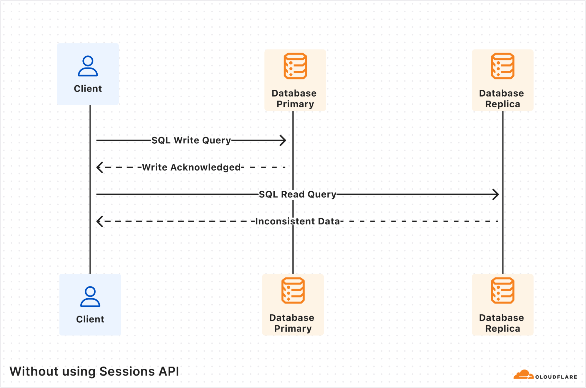
The Client, a user Worker, sends a D1 write query that gets processed by the database primary and gets the results back. However, the subsequent read query ends up being processed by a database replica. If the database replica is lagging far enough behind the database primary, such that it does not yet include the first write query, then the returned results will be inconsistent, and probably incorrect for your application business logic.


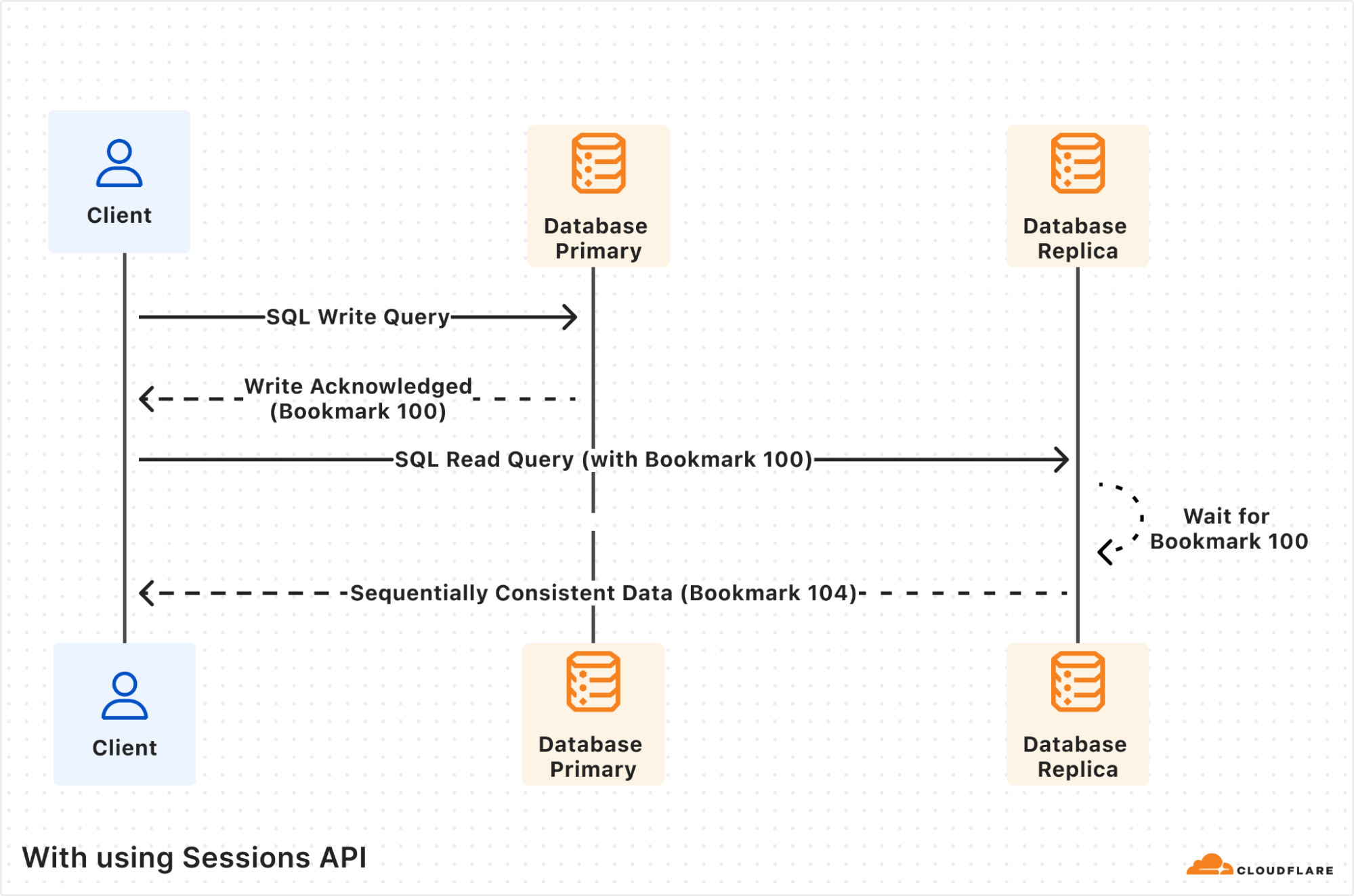
Using the Sessions API fixes the inconsistency issue. The first write query is again processed by the database primary, and this time the response includes “Bookmark 100”. The session object will store this bookmark for you transparently.

The subsequent read query is processed by database replica as before, but now since the query includes the previously received “Bookmark 100”, the database replica will wait until its database copy is at least up-to-date as “Bookmark 100”. Only once it’s up-to-date, the read query will be processed and the results returned, including the replica’s latest bookmark “Bookmark 104”.

Notice that the returned bookmark for the read query is “Bookmark 104”, which is different from the one passed in the query request. This can happen if there were other writes from other client requests that also got replicated to the database replica in-between the two queries our own client executed.

Enabling read replication

To start using D1 read replication:

  1. Update your Worker to use the D1 Sessions API to tell D1 what queries are part of the same database session. The Sessions API works with databases that do not have read replication enabled as well, so it’s safe to ship this code even before you enable replicas. Here’s an example.

  2. Enable replicas for your database via Cloudflare dashboard > Select D1 database > Settings.

D1 read replication is built into D1, and you don’t pay extra storage or compute costs for replicas. You incur the exact same D1 usage with or without replicas, based on rows_read and rows_written by your queries. Unlike other traditional database systems with replication, you don’t have to manually create replicas, including where they run, or decide how to route requests between the primary database and read replicas. Cloudflare handles this when using the Sessions API while ensuring sequential consistency.

Since D1 read replication is in beta, we recommend trying D1 read replication on a non-production database first, and migrate to your production workloads after validating read replication works for your use case.

If you don’t have a D1 database and want to try out D1 read replication, create a test database in the Cloudflare dashboard.

Observing your replicas

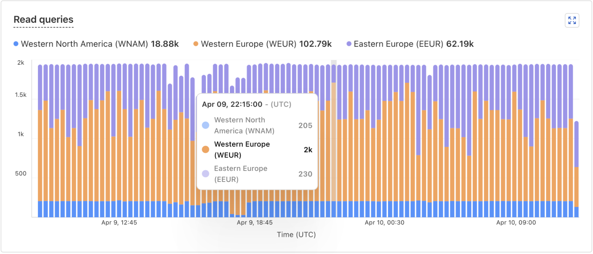
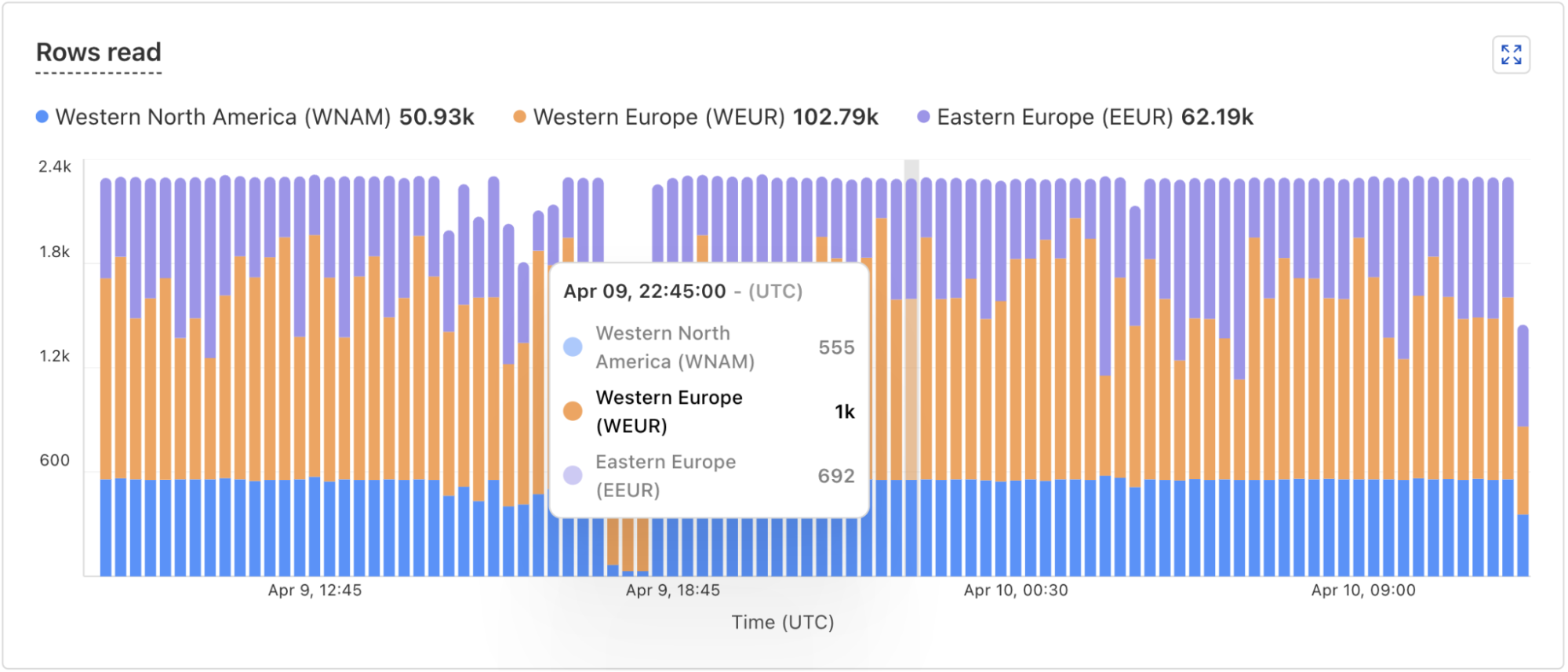
Once you’ve enabled D1 read replication, read queries will start to be processed by replica database instances. The response of each query includes information in the nested meta object relevant to read replication, like served_by_region and served_by_primary. The first denotes the region of the database instance that processed the query, and the latter will be true if-and-only-if your query was processed by the primary database instance.

In addition, the D1 dashboard overview for a database now includes information about the database instances handling your queries. You can see how many queries are handled by the primary instance or by a replica, and a breakdown of the queries processed by region. The example screenshots below show graphs displaying the number of queries executed and number of rows read by each region.


Under the hood: how D1 read replication is implemented

D1 is implemented on top of SQLite-backed Durable Objects running on top of Cloudflare’s Storage Relay Service.


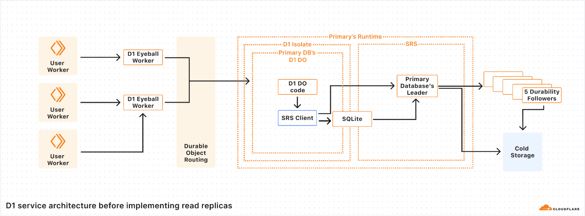
D1 is structured with a 3-layer architecture.  First is the binding API layer that runs in the customer’s Worker.  Next is a stateless Worker layer that routes requests based on database ID to a layer of Durable Objects that handle the actual SQL operations behind D1.  This is similar to how most applications using Cloudflare Workers and Durable Objects are structured.

For a non-replicated database, there is exactly one Durable Object per database.  When a user’s Worker makes a request with the D1 binding for the database, that request is first routed to a D1 Worker running in the same location as the user’s Worker.  The D1 Worker figures out which D1 Durable Object backs the user’s D1 database and fetches an RPC stub to that Durable Object.  The Durable Objects routing layer figures out where the Durable Object is located, and opens an RPC connection to it.  Finally, the D1 Durable Object then handles the query on behalf of the user’s Worker using the Durable Objects SQL API.

In the Durable Objects SQL API, all queries go to a SQLite database on the local disk of the server where the Durable Object is running.  Durable Objects run SQLite in WAL mode.  In WAL mode, every write query appends to a write-ahead log (the WAL).  As SQLite appends entries to the end of the WAL file, a database-specific component called the Storage Relay Service leader synchronously replicates the entries to 5 durability followers on servers in different datacenters.  When a quorum (at least 3 out of 5) of the durability followers acknowledge that they have safely stored the data, the leader allows SQLite’s write queries to commit and opens the Durable Object’s output gate, so that the Durable Object can respond to requests.

Our implementation of WAL mode allows us to have a complete log of all of the committed changes to the database. This enables a couple of important features in SQLite-backed Durable Objects and D1:

  • We identify each write with a Lamport timestamp we call a bookmark.

  • We construct databases anywhere in the world by downloading all of the WAL entries from cold storage and replaying each WAL entry in order.

  • We implement Point-in-time recovery (PITR) by replaying WAL entries up to a specific bookmark rather than to the end of the log.

Unfortunately, having the main data structure of the database be a log is not ideal.  WAL entries are in write order, which is often neither convenient nor fast.  In order to cut down on the overheads of the log, SQLite checkpoints the log by copying the WAL entries back into the main database file.  Read queries are serviced directly by SQLite using files on disk — either the main database file for checkpointed queries, or the WAL file for writes more recent than the last checkpoint.  Similarly, the Storage Relay Service snapshots the database to cold storage so that we can replay a database by downloading the most recent snapshot and replaying the WAL from there, rather than having to download an enormous number of individual WAL entries.

WAL mode is the foundation for implementing read replication, since we can stream writes to locations other than cold storage in real time.


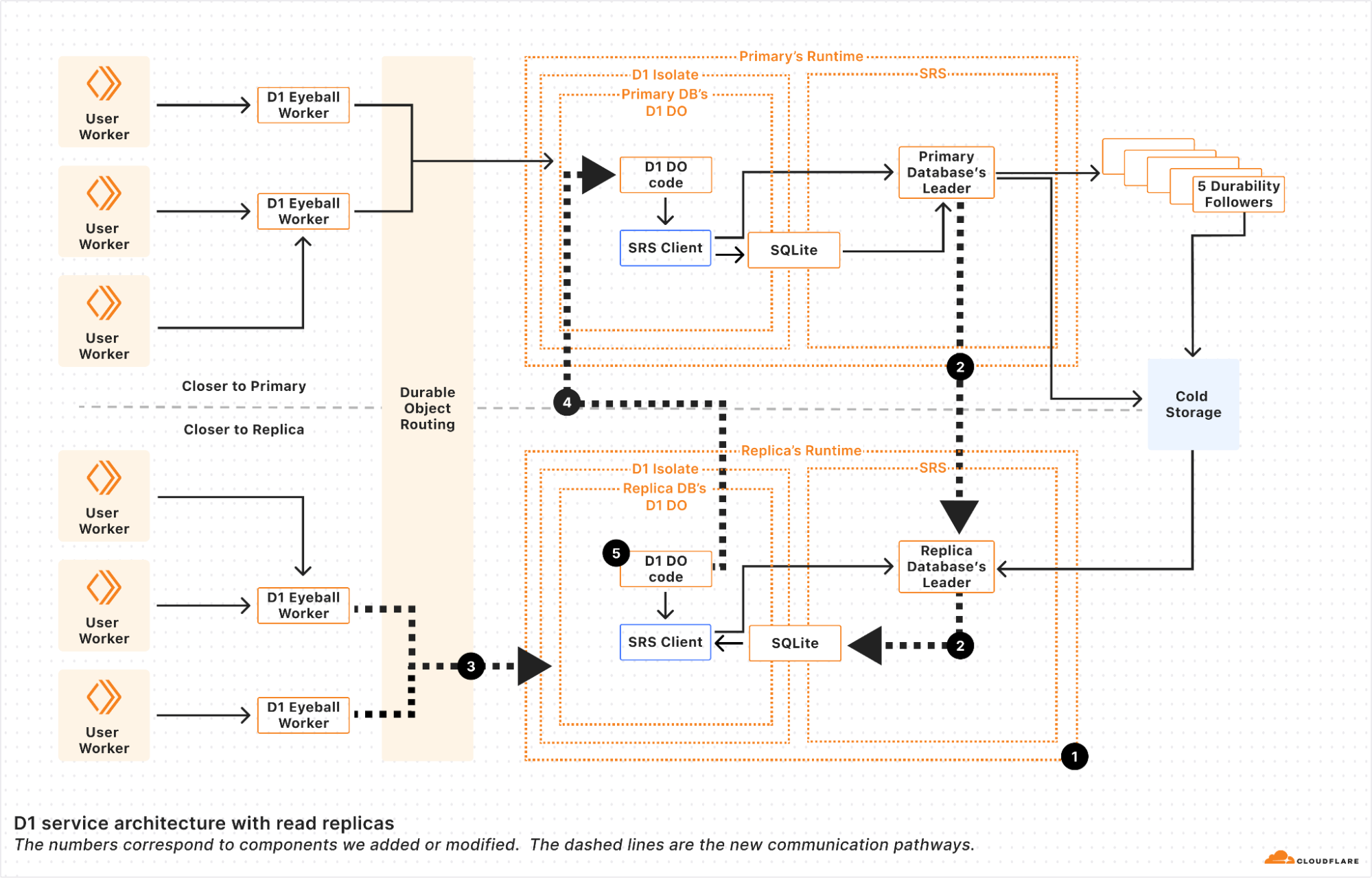
We implemented read replication in 5 major steps.

First, we made it possible to make replica Durable Objects with a read-only copy of the database.  These replica objects boot by fetching the latest snapshot and replaying the log from cold storage to whatever bookmark primary database’s leader last committed. This basically gave us point-in-time replicas, since without continuous updates, the replicas never updated until the Durable Object restarted.

Second, we registered the replica leader with the primary’s leader so that the primary leader sends the replicas every entry written to the WAL at the same time that it sends the WAL entries to the durability followers.  Each of the WAL entries is marked with a bookmark that uniquely identifies the WAL entry in the sequence of WAL entries.  We’ll use the bookmark later.

Note that since these writes are sent to the replicas before a quorum of durability followers have confirmed them, the writes are actually unconfirmed writes, and the replica leader must be careful to keep the writes hidden from the replica Durable Object until they are confirmed.  The replica leader in the Storage Relay Service does this by implementing enough of SQLite’s WAL-index protocol, so that the unconfirmed writes coming from the primary leader look to SQLite as though it’s just another SQLite client doing unconfirmed writes.  SQLite knows to ignore the writes until they are confirmed in the log.  The upshot of this is that the replica leader can write WAL entries to the SQLite WAL immediately, and then “commit” them when the primary leader tells the replica that the entries have been confirmed by durability followers.

One neat thing about this approach is that writes are sent from the primary to the replica as quickly as they are generated by the primary, helping to minimize lag between replicas.  In theory, if the write query was proxied through a replica to the primary, the response back to the replica will arrive at almost the same time as the message that updates the replica.  In such a case, it looks like there’s no replica lag at all!

In practice, we find that replication is really fast.  Internally, we measure confirm lag, defined as the time from when a primary confirms a change to when the replica confirms a change.  The table below shows the confirm lag for two D1 databases whose primaries are in different regions.

Replica Region

Database A

(Primary region: ENAM)

Database B
(Primary region: WNAM)

ENAM

N/A

30 ms

WNAM

45 ms

N/A

WEUR

55 ms

75 ms

EEUR

67 ms

75 ms

Confirm lag for 2 replicated databases.  N/A means that we have no data for this combination.  The region abbreviations are the same ones used for Durable Object location hints.

The table shows that confirm lag is correlated with the network round-trip time between the data centers hosting the primary databases and their replicas.  This is clearly visible in the difference between the confirm lag for the European replicas of the two databases.  As airline route planners know, EEUR is appreciably further away from ENAM than WNAM, but from WNAM, both European regions (WEUR and EEUR) are about equally as far away.  We see that in our replication numbers.

The exact placement of the D1 database in the region matters too.  Regions like ENAM and WNAM are quite large in themselves.  Database A’s placement in ENAM happens to be further away from most data centers in WNAM compared to database B’s placement in WNAM relative to the ENAM data centers.  As such, database B sees slightly lower confirm lag.

Try as we might, we can’t beat the speed of light!

Third, we updated the Durable Object routing system to be aware of Durable Object replicas.  When read replication is enabled on a Durable Object, two things happen.  First, we create a set of replicas according to a replication policy.  The current replication policy that D1 uses is simple: a static set of replicas in every region that D1 supports.  Second, we turn on a routing policy for the Durable Object.  The current policy that D1 uses is also simple: route to the Durable Object replica in the region close to where the user request is.  With this step, we have updateable read-only replicas, and can route requests to them!

Fourth, we updated D1’s Durable Object code to handle write queries on replicas. D1 uses SQLite to figure out whether a request is a write query or a read query.  This means that the determination of whether something is a read or write query happens after the request is routed.  Read replicas will have to handle write requests!  We solve this by instantiating each replica D1 Durable Object with a reference to its primary.  If the D1 Durable Object determines that the query is a write query, it forwards the request to the primary for the primary to handle. This happens transparently, keeping the user code simple.

As of this fourth step, we can handle read and write queries at every copy of the D1 Durable Object, whether it’s a primary or not.  Unfortunately, as outlined above, if a user’s requests get routed to different read replicas, they may see different views of the database, leading to a very weak consistency model.  So the last step is to implement the Sessions API across the D1 Worker and D1 Durable Object.  Recall that every WAL entry is marked with a bookmark.  These bookmarks uniquely identify a point in (logical) time in the database.  Our bookmarks are strictly monotonically increasing; every write to a database makes a new bookmark with a value greater than any other bookmark for that database.

Using bookmarks, we implement the Sessions API with the following algorithm split across the D1 binding implementation, the D1 Worker, and D1 Durable Object.

First up in the D1 binding, we have code that creates the D1DatabaseSession object and code within the D1DatabaseSession object to keep track of the latest bookmark.

// D1Binding is the binding code running within the user's Worker
// that provides the existing D1 Workers API and the new withSession method.
class D1Binding {
  // Injected by the runtime to the D1 Binding.
  d1Service: D1ServiceBinding

  function withSession(initialBookmark) {
    return D1DatabaseSession(this.d1Service, this.databaseId, initialBookmark);
  }
}

// D1DatabaseSession holds metadata about the session, most importantly the
// latest bookmark we know about for this session.
class D1DatabaseSession {
  constructor(d1Service, databaseId, initialBookmark) {
    this.d1Service = d1Service;
    this.databaseId = databaseId;
    this.bookmark = initialBookmark;
  }

  async exec(query) {
    // The exec method in the binding sends the query to the D1 Worker
    // and waits for the the response, updating the bookmark as
    // necessary so that future calls to exec use the updated bookmark.
    var resp = await this.d1Service.handleUserQuery(databaseId, query, bookmark);
    if (isNewerBookmark(this.bookmark, resp.bookmark)) {
      this.bookmark = resp.bookmark;
    }
    return resp;
  }

  // batch and other SQL APIs are implemented similarly.
}

The binding code calls into the D1 stateless Worker (d1Service in the snippet above), which figures out which Durable Object to use, and proxies the request to the Durable Object.

class D1Worker {
  async handleUserQuery(databaseId, query) {
    var doId = /* look up Durable Object for databaseId */;
    return await this.D1_DO.get(doId).handleWorkerQuery(query, bookmark)
  }
}

Finally, we reach the Durable Objects layer, which figures out how to actually handle the request.

class D1DurableObject {
  async handleWorkerQuery(queries, bookmark) {
    var bookmark = bookmark ?? "first-primary";
    var results = {};

    if (this.isPrimaryDatabase()) {
      // The primary always has the latest data so we can run the
      // query without checking the bookmark.
      var result = /* execute query directly */;
      bookmark = getCurrentBookmark();
      results = result;
    } else {
      // This is running on a replica.
      if (bookmark === "first-primary" || isWriteQuery(query)) {
        // The primary must handle this request, so we'll proxy the
        // request to the primary.
        var resp = await this.primary.handleWorkerQuery(query, bookmark);
        bookmark = resp.bookmark;
        results = resp.results;
      } else {
        // The replica can handle this request, but only after the
        // database is up-to-date with the bookmark.
        if (bookmark !== "first-unconstrained") {
          await waitForBookmark(bookmark);
        }
        var result = /* execute query locally */;
        bookmark = getCurrentBookmark();
        results = result;
      }
    }
    return { results: results, bookmark: bookmark };
  }
}

The D1 Durable Object first figures out if this instance can handle the query, or if the query needs to be sent to the primary.  If the Durable Object can execute the query, it ensures that we execute the query with a bookmark at least as up-to-date as the bookmark requested by the binding.

The upshot is that the three pieces of code work together to ensure that all of the queries in the session see the database in a sequentially consistent order, because each new query will be blocked until it has seen the results of previous queries within the same session.

Conclusion

D1’s new read replication feature is a significant step towards making globally distributed databases easier to use without sacrificing consistency. With automatically provisioned replicas in every region, your applications can now serve read queries faster while maintaining strong sequential consistency across requests, and keeping your application Worker code simple.

We’re excited for developers to explore this feature and see how it improves the performance of your applications. The public beta is just the beginning—we’re actively refining and expanding D1’s capabilities, including evolving replica placement policies, and your feedback will help shape what’s next.

Note that the Sessions API is only available through the D1 Worker Binding for now, and support for the HTTP REST API will follow soon.

Try out D1 read replication today by clicking the “Deploy to Cloudflare” button, check out documentation and examples, and let us know what you build in the D1 Discord channel!

Building Vectorize, a distributed vector database, on Cloudflare’s Developer Platform

Post Syndicated from Jérôme Schneider original https://blog.cloudflare.com/building-vectorize-a-distributed-vector-database-on-cloudflare-developer-platform

Vectorize is a globally distributed vector database that enables you to build full-stack, AI-powered applications with Cloudflare Workers. Vectorize makes querying embeddings — representations of values or objects like text, images, audio that are designed to be consumed by machine learning models and semantic search algorithms — faster, easier and more affordable.

In this post, we dive deep into how we built Vectorize on Cloudflare’s Developer Platform, leveraging Cloudflare’s global network, Cache, Workers, R2, Queues, Durable Objects, and container platform.

What is a vector database?

A vector database is a queryable store of vectors. A vector is a large array of numbers called vector dimensions.

A vector database has a similarity search query: given an input vector, it returns the vectors that are closest according to a specified metric, potentially filtered on their metadata.

Vector databases are used to power semantic search, document classification, and recommendation and anomaly detection, as well as contextualizing answers generated by LLMs (Retrieval Augmented Generation, RAG).

Why do vectors require special database support?

Conventional data structures like B-trees, or binary search trees expect the data they index to be cheap to compare and to follow a one-dimensional linear ordering. They leverage this property of the data to organize it in a way that makes search efficient. Strings, numbers, and booleans are examples of data featuring this property.

Because vectors are high-dimensional, ordering them in a one-dimensional linear fashion is ineffective for similarity search, as the resulting ordering doesn’t capture the proximity of vectors in the high-dimensional space. This phenomenon is often referred to as the curse of dimensionality.

In addition to this, comparing two vectors using distance metrics useful for similarity search is a computationally expensive operation, requiring vector-specific techniques for databases to overcome.

Query processing architecture

Vectorize builds upon Cloudflare’s global network to bring fast vector search close to its users, and relies on many components to do so.

These are the Vectorize components involved in processing vector queries.


Vectorize runs in every Cloudflare data center, on the infrastructure powering Cloudflare Workers. It serves traffic coming from Worker bindings as well as from the Cloudflare REST API through our API Gateway.

Each query is processed on a server in the data center in which it enters, picked in a fashion that spreads the load across all servers of that data center.

The Vectorize DB Service (a Rust binary) running on that server processes the query by reading the data for that index on R2, Cloudflare’s object storage. It does so by reading through Cloudflare’s Cache to speed up I/O operations.

Searching vectors, and indexing them to speed things up

Being a vector database, Vectorize features a similarity search query: given an input vector, it returns the K vectors that are closest according to a specified metric.

Conceptually, this similarity search consists of 3 steps:

  1. Evaluate the proximity of the query vector with every vector present in the index.

  2. Sort the vectors based on their proximity “score”.

  3. Return the top matches.

While this method is accurate and effective, it is computationally expensive and does not scale well to indexes containing millions of vectors (see Why do vectors require special database support? above).

To do better, we need to prune the search space, that is, avoid scanning the entire index for every query.

For this to work, we need to find a way to discard vectors we know are irrelevant for a query, while focusing our efforts on those that might be relevant.

Indexing vectors with IVF

Vectorize prunes the search space for a query using an indexing technique called IVF, Inverted File Index.

IVF clusters the index vectors according to their relative proximity. For each cluster, it then identifies its centroid, the center of gravity of that cluster, a high-dimensional point minimizing the distance with every vector in the cluster.


Once the list of centroids is determined, each centroid is given a number. We then structure the data on storage by placing each vector in a file named like the centroid it is closest to.

When processing a query, we then can then focus on relevant vectors by looking only in the centroid files closest to that query vector, effectively pruning the search space.


Compressing vectors with PQ

Vectorize supports vectors of up to 1536 dimensions. At 4 bytes per dimension (32 bits float), this means up to 6 KB per vector. That’s 6 GB of uncompressed vector data per million vectors that we need to fetch from storage and put in memory.

To process multi-million vector indexes while limiting the CPU, memory, and I/O required to do so, Vectorize uses a dimensionality reduction technique called PQ (Product Quantization). PQ compresses the vectors data in a way that retains most of their specificity while greatly reducing their size — a bit like down sampling a picture to reduce the file size, while still being able to tell precisely what’s in the picture — enabling Vectorize to efficiently perform similarity search on these lighter vectors.

In addition to storing the compressed vectors, their original data is retained on storage as well, and can be requested through the API; the compressed vector data is used only to speed up the search.

Approximate nearest neighbor search and result accuracy refining

By pruning the search space and compressing the vector data, we’ve managed to increase the efficiency of our query operation, but it is now possible to produce a set of matches that is different from the set of true closest matches. We have traded result accuracy for speed by performing an approximate nearest neighbor search, reaching an accuracy of ~80%.

To boost the result accuracy up to over 95%, Vectorize then performs a result refinement pass on the top approximate matches using uncompressed vector data, and returns the best refined matches.

Eventual consistency and snapshot versioning

Whenever you query your Vectorize index, you are guaranteed to receive results which are read from a consistent, immutable snapshot — even as you write to your index concurrently. Writes are applied in strict order of their arrival in our system, and they are funneled into an asynchronous process. We update the index files by reading the old version, making changes, and writing this updated version as a new object in R2. Each index file has its own version number, and can be updated independently of the others. Between two versions of the index we may update hundreds or even thousands of IVF and metadata index files, but even as we update the files, your queries will consistently use the current version until it is time to switch.

Each IVF and metadata index file has its own version. The list of all versioned files which make up the snapshotted version of the index is contained within a manifest file. Each version of the index has its own manifest. When we write a new manifest file based on the previous version, we only need to update references to the index files which were modified; if there are files which weren’t modified, we simply keep the references to the previous version.

We use a root manifest as the authority of the current version of the index. This is the pivot point for changes. The root manifest is a copy of a manifest file from a particular version, which is written to a deterministic location (the root of the R2 bucket for the index). When our async write process has finished processing vectors, and has written all new index files to R2, we commit by overwriting the current root manifest with a copy of the new manifest. PUT operations in R2 are atomic, so this effectively makes our updates atomic. Once the manifest is updated, Vectorize DB Service instances running on our network will pick it up, and use it to serve reads.

Because we keep past versions of index and manifest files, we effectively maintain versioned snapshots of your index. This means we have a straightforward path towards building a point-in-time recovery feature (similar to D1’s Time Travel feature).

You may have noticed that because our write process is asynchronous, this means Vectorize is eventually consistent — that is, there is a delay between the successful completion of a request writing on the index, and finally seeing those updates reflected in queries.  This isn’t always ideal for all data storage use cases. For example, imagine two users using an online ticket reservation application for airline tickets, where both users buy the same seat — one user will successfully reserve the ticket, and the other will eventually get an error saying the seat was taken, and they need to choose again. Because a vector index is not typically used as a primary database for these transactional use cases, we decided eventual consistency was a worthy trade off in order to ensure Vectorize queries would be fast, high-throughput, and cheap even as the size of indexes grew into the millions.

Coordinating distributed writes: it’s just another block in the WAL

In the section above, we touched on our eventually consistent, asynchronous write process. Now we’ll dive deeper into our implementation. 

The WAL

A write ahead log (WAL) is a common technique for making atomic and durable writes in a database system. Vectorize’s WAL is implemented with SQLite in Durable Objects.

In Vectorize, the payload for each update is given an ID, written to R2, and the ID for that payload is handed to the WAL Durable Object which persists it as a “block.” Because it’s just a pointer to the data, the blocks are lightweight records of each mutation.

Durable Objects (DO) have many benefits — strong transactional guarantees, a novel combination of compute and storage, and a high degree of horizontal scale — but individual DOs are small allotments of memory and compute. However, the process of updating the index for even a single mutation is resource intensive — a single write may include thousands of vectors, which may mean reading and writing thousands of data files stored in R2, and storing a lot of data in memory. This is more than what a single DO can handle.

So we designed the WAL to leverage DO’s strengths and made it a coordinator. It controls the steps of updating the index by delegating the heavy lifting to beefier instances of compute resources (which we call “Executors”), but uses its transactional properties to ensure the steps are done with strong consistency. It safeguards the process from rogue or stalled executors, and ensures the WAL processing continues to move forward. DOs are easy to scale, so we create a new DO instance for each Vectorize index.


WAL Executor

The executors run from a single pool of compute resources, shared by all WALs. We use a simple producer-consumer pattern using Cloudflare Queues. The WAL enqueues a request, and executors poll the queue. When they get a request, they call an API on the WAL requesting to be assigned to the request.

The WAL ensures that one and only one executor is ever assigned to that write. As the executor writes, the index files and the updated manifest are written in R2, but they are not yet visible. The final step is for the executor to call another API on the WAL to commit the change — and this is key — it passes along the updated manifest. The WAL is responsible for overwriting the root manifest with the updated manifest. The root manifest is the pivot point for atomic updates: once written, the change is made visible to Vectorize’s database service, and the updated data will appear in queries.

From the start, we designed this process to account for non-deterministic errors. We focused on enumerating failure modes first, and only moving forward with possible design options after asserting they handled the possibilities for failure. For example, if an executor stalls, the WAL finds a new executor. If the first executor comes back, the coordinator will reject its attempt to commit the update. Even if that first executor is working on an old version which has already been written, and writes new index files and a new manifest to R2, they will not overwrite the files written from the committed version.

Batching updates

Now that we have discussed the general flow, we can circle back to one of our favorite features of the WAL. On the executor, the most time-intensive part of the write process is reading and writing many files from R2. Even with making our reads and writes concurrent to maximize throughput, the cost of updating even thousands of vectors within a single file is dwarfed by the total latency of the network I/O. Therefore it is more efficient to maximize the number of vectors processed in a single execution.

So that is what we do: we batch discrete updates. When the WAL is ready to request work from an executor, it will get a chunk of “blocks” off the WAL, starting with the next un-written block, and maintaining the sequence of blocks. It will write a new “batch” record into the SQLite table, which ties together that sequence of blocks, the version of the index, and the ID of the executor assigned to the batch.

Users can batch multiple vectors to update in a single insert or upsert call. Because the size of each update can vary, the WAL adaptively calculates the optimal size of its batch to increase throughput. The WAL will fit as many upserted vectors as possible into a single batch by counting the number of updates represented by each block. It will batch up to 200,000 vectors at once (a value we arrived at after our own testing) with a limit of 1,000 blocks. With this throughput, we have been able to quickly load millions of vectors into an index (with upserts of 5,000 vectors at a time). Also, the WAL does not pause itself to collect more writes to batch — instead, it begins processing a write as soon as it arrives. Because the WAL only processes one batch at a time, this creates a natural pause in its workflow to batch up writes which arrive in the meantime.

Retraining the index

The WAL also coordinates our process for retraining the index. We occasionally re-train indexes to ensure the mapping of IVF centroids best reflects the current vectors in the index. This maintains the high accuracy of the vector search.

Retraining produces a completely new index. All index files are updated; vectors have been reshuffled across the index space. For this reason, all indexes have a second version stamp — which we call the generation — so that we can differentiate between retrained indexes. 

The WAL tracks the state of the index, and controls when the training is started. We have a second pool of processes called “trainers.” The WAL enqueues a request on a queue, then a trainer picks up the request and it begins training.

Training can take a few minutes to complete, but we do not pause writes on the current generation. The WAL will continue to handle writes as normal. But the training runs from a fixed snapshot of the index, and will become out-of-date as the live index gets updated in parallel. Once the trainer has completed, it signals the WAL, which will then start a multi-step process to switch to the new generation. It enters a mode where it will continue to record writes in the WAL, but will stop making those writes visible on the current index. Then it will begin catching up the retrained index with all of the updates that came in since it started. Once it has caught up to all data present in the index when the trainer signaled the WAL, it will switch over to the newly retrained index. This prevents the new index from appearing to “jump back in time.” All subsequent writes will be applied to that new index.

This is all modeled seamlessly with the batch record. Because it associates the index version with a range of WAL blocks, multiple batches can span the same sequence of blocks as long as they belong to different generations. We can say this another way: a single WAL block can be associated with many batches, as long as these batches are in different generations. Conceptually, the batches act as a second WAL layered over the WAL blocks.

Indexing and filtering metadata

Vectorize supports metadata filters on vector similarity queries. This allows a query to focus the vector similarity search on a subset of the index data, yielding matches that would otherwise not have been part of the top results.

For instance, this enables us to query for the best matching vectors for color: “blue” and category: ”robe”.

Conceptually, what needs to happen to process this example query is:

  • Identify the set of vectors matching color: “blue” by scanning all metadata.

  • Identify the set of vectors matching category: “robe” by scanning all metadata.

  • Intersect both sets (boolean AND in the filter) to identify vectors matching both the color and category filter.

  • Score all vectors in the intersected set, and return the top matches.

While this method works, it doesn’t scale well. For an index with millions of vectors, processing the query that way would be very resource intensive. What’s worse, it prevents us from using our IVF index to identify relevant vector data, forcing us to compute a proximity score on potentially millions of vectors if the filtered set of vectors is large.

To do better, we need to prune the metadata search space by indexing it like we did for the vector data, and find a way to efficiently join the vector sets produced by the metadata index with our IVF vector index.

Indexing metadata with Chunked Sorted List Indexes

Vectorize maintains one metadata index per filterable property. Each filterable metadata property is indexed using a Chunked Sorted List Index.

A Chunked Sorted List Index is a sorted list of all distinct values present in the data for a filterable property, with each value mapped to the set of vector IDs having that value. This enables Vectorize to binary search a value in the metadata index in O(log n) complexity, in other words about as fast as search can be on a large dataset.

Because it can become very large on big indexes, the sorted list is chunked in pieces matching a target weight in KB to keep index state fetches efficient.


A lightweight chunk descriptor list is maintained in the index manifest, keeping track of the list chunks and their lower/upper values. This chunk descriptor list can be binary searched to identify which chunk would contain the searched metadata value.

Once the candidate chunk is identified, Vectorize fetches that chunk from index data and binary searches it to take the set of vector IDs matching a metadata value if found, or an empty set if not found.


We identify the matching vector set this way for every predicate in the metadata filter of the query, then intersect the sets in memory to determine the final set of vectors matched by the filters.

This is just half of the query being processed. We now need to identify the vectors most similar to the query vector, within those matching the metadata filters.

Joining the metadata and vector indexes

A vector similarity query always comes with an input vector. We can rank all centroids of our IVF vector index based on their proximity with that query vector.

The vector set matched by the metadata filters contains for each vector its ID and IVF centroid number.

From this, Vectorize derives the number of vectors matching the query filters per IVF centroid, and determines which and how many top-ranked IVF centroids need to be scanned according to the number of matches the query asks for.

Vectorize then performs the IVF-indexed vector search (see the section Searching Vectors, and indexing them to speed things up above) by considering only the vectors in the filtered metadata vector set while doing so.

Because we’re effectively pruning the vector search space using metadata filters, filtered queries can often be faster than their unfiltered equivalent.

Query performance

The performance of a system is measured in terms of latency and throughput.

Latency is a measure relative to individual queries, evaluating the time it takes for a query to be processed, usually expressed in milliseconds. It is what an end user perceives as the “speed” of the service, so a lower latency is desirable.

Throughput is a measure relative to an index, evaluating the number of queries it can process concurrently over a period of time, usually expressed in requests per second or RPS. It is what enables an application to scale to thousands of simultaneous users, so a higher throughput is desirable.

Vectorize is designed for great index throughput and optimized for low query latency to deliver great performance for demanding applications. Check out our benchmarks.

Query latency optimization

As a distributed database keeping its data state on blob storage, Vectorize’s latency is primarily driven by the fetch of index data, and relies heavily on Cloudflare’s network of caches as well as individual server RAM cache to keep latency low.

Because Vectorize data is snapshot versioned, (see Eventual consistency and snapshot versioning above), each version of the index data is immutable and thus highly cacheable, increasing the latency benefits Vectorize gets from relying on Cloudflare’s cache infrastructure.

To keep the index data lean, Vectorize uses techniques to reduce its weight. In addition to Product Quantization (see Compressing vectors with PQ above), index files use a space-efficient binary format optimized for runtime performance that Vectorize is able to use without parsing, once fetched.

Index data is fragmented in a way that minimizes the amount of data required to process a query. Auxiliary indexes into that data are maintained to limit the amount of fragments to fetch, reducing overfetch by jumping straight to the relevant piece of data on mass storage.

Vectorize boosts all vector proximity computations by leveraging SIMD CPU instructions, and by organizing the vector search in 2 passes, effectively balancing the latency/result accuracy ratio (see Approximate nearest neighbor search and result accuracy refining above).

When used via a Worker binding, each query is processed close to the server serving the worker request, and thus close to the end user, minimizing the network-induced latency between the end user, the Worker application, and Vectorize.

Query throughput

Vectorize runs in every Cloudflare data center, on thousands of servers across the world.

Thanks to the snapshot versioning of every index’s data, every server is simultaneously able to serve the index concurrently, without contention on state.

This means that a Vectorize index elastically scales horizontally with its distributed traffic, providing very high throughput for the most demanding Worker applications.

Increased index size

We are excited that our upgraded version of Vectorize can support a maximum of 5 million vectors, which is a 25x improvement over the limit in beta (200,000 vectors). All the improvements we discussed in this blog post contribute to this increase in vector storage. Improved query performance and throughput comes with this increase in storage as well.

However, 5 million may be constraining for some use cases. We have already heard this feedback. The limit falls out of the constraints of building a brand new globally distributed stateful service, and our desire to iterate fast and make Vectorize generally available so builders can confidently leverage it in their production apps.

We believe builders will be able to leverage Vectorize as their primary vector store, either with a single index or by sharding across multiple indexes. But if this limit is too constraining for you, please let us know. Tell us your use case, and let’s see if we can work together to make Vectorize work for you.

Try it now!

Every developer on a free plan can give Vectorize a try. You can visit our developer documentation to get started.

If you’re looking for inspiration on what to build, see the semantic search tutorial that combines Workers AI and Vectorize for document search, running entirely on Cloudflare. Or an example of how to combine OpenAI and Vectorize to give an LLM more context and dramatically improve the accuracy of its answers.

And if you have questions about how to use Vectorize for our product & engineering teams, or just want to bounce an idea off of other developers building on Workers AI, join the #vectorize and #workers-ai channels on our Developer Discord.

Cloudflare Integrations Marketplace introduces three new partners: Sentry, Momento and Turso

Post Syndicated from Tanushree Sharma original http://blog.cloudflare.com/cloudflare-integrations-marketplace-new-partners-sentry-momento-turso/

Cloudflare Integrations Marketplace introduces three new partners: Sentry, Momento and Turso

Cloudflare Integrations Marketplace introduces three new partners: Sentry, Momento and Turso

Building modern full-stack applications requires connecting to many hosted third party services, from observability platforms to databases and more. All too often, this means spending time doing busywork, managing credentials and writing glue code just to get started. This is why we’re building out the Cloudflare Integrations Marketplace to allow developers to easily discover, configure and deploy products to use with Workers.

Earlier this year, we introduced integrations with Supabase, PlanetScale, Neon and Upstash. Today, we are thrilled to introduce our newest additions to Cloudflare’s Integrations Marketplace – Sentry, Turso and Momento.

Let's take a closer look at some of the exciting integration providers that are now part of the Workers Integration Marketplace.

Improve performance and reliability by connecting Workers to Sentry

When your Worker encounters an error you want to know what happened and exactly what line of code triggered it. Sentry is an application monitoring platform that helps developers identify and resolve issues in real-time.

The Workers and Sentry integration automatically sends errors, exceptions and console.log() messages from your Worker to Sentry with no code changes required. Here’s how it works:

  1. You enable the integration from the Cloudflare Dashboard.
  2. The credentials from the Sentry project of your choice are automatically added to your Worker.
  3. You can configure sampling to control the volume of events you want sent to Sentry. This includes selecting the sample rate for different status codes and exceptions.
  4. Cloudflare deploys a Tail Worker behind the scenes that contains all the logic needed to capture and send data to Sentry.
  5. Like magic, errors, exceptions, and log messages are automatically sent to your Sentry project.

In the future, we’ll be improving this integration by adding support for uploading source maps and stack traces so that you can pinpoint exactly which line of your code caused the issue. We’ll also be tying in Workers deployments with Sentry releases to correlate new versions of your Worker with events in Sentry that help pinpoint problematic deployments. Check out our developer documentation for more information.

Develop at the Data Edge with Turso + Workers

Turso is an edge-hosted, distributed database based on libSQL, an open-source fork of SQLite. Turso focuses on providing a global service that minimizes query latency (and thus, application latency!). It’s perfect for use with Cloudflare Workers – both compute and data are served close to users.

Turso follows the model of having one primary database with replicas that are located globally, close to users. Turso automatically routes requests to a replica closest to where the Worker was invoked. This model works very efficiently for read heavy applications since read requests can be served globally. If you’re running an application that has heavy write workloads, or want to cut down on replication costs, you can run Turso with just the primary instance and use Smart Placement to speed up queries.

The Turso and Workers integration automatically pulls in Turso API credentials and adds them as secrets to your Worker, so that you can start using Turso by simply establishing a connection using the libsql SDK. Get started with the Turso and Workers Integration today by heading to our developer documentation.

Cache responses from data stores with Momento

Momento Cache is a low latency serverless caching solution that can be used on top of relational databases, key-value databases or object stores to get faster load times and better performance. Momento abstracts details like scaling, warming and replication so that users can deploy cache in a matter of minutes.

The Momento and Workers integration automatically pulls in your Momento API key using an OAuth2 flow. The Momento API key is added as a secret in Workers and, from there, you can start using the Momento SDK in Workers. Head to our developer documentation to learn more and use the Momento and Workers integration!

Try integrations out today

We want to give you back time, so that you can focus less on configuring and connecting third party tools to Workers and spend more time building. We’re excited to see what you build with integrations. Share your projects with us on Twitter (@CloudflareDev) and stay tuned for more exciting updates as we continue to grow our Integrations Marketplace!

If you would like to build an integration with Cloudflare Workers, fill out the integration request form and we’ll be in touch.

Performance isolation in a multi-tenant database environment

Post Syndicated from Justin Kwan original https://blog.cloudflare.com/performance-isolation-in-a-multi-tenant-database-environment/

Performance isolation in a multi-tenant database environment

Performance isolation in a multi-tenant database environment

Operating at Cloudflare scale means that across the technology stack we spend a great deal of time handling different load conditions. In this blog post we talk about how we solved performance difficulties with our Postgres clusters. These clusters support a large number of tenants and highly variable load conditions leading to the need to isolate activity to prevent tenants taking too much time from others. Welcome to real-world, large database cluster management!

As an intern at Cloudflare I got to work on improving how our database clusters behave under load and open source the resulting code.

Cloudflare operates production Postgres clusters across multiple regions in data centers. Some of our earliest service offerings, such as our DNS Resolver, Firewall, and DDoS Protection, depend on our Postgres clusters’ high availability for OLTP workloads. The high availability cluster manager, Stolon, is employed across all clusters to independently control and replicate data across Postgres instances and elect Postgres leaders and failover under high load scenarios.

PgBouncer and HAProxy act as the gateway layer in each cluster. Each tenant acquires client-side connections from PgBouncer instead of Postgres directly. PgBouncer holds a pool of maximum server-side connections to Postgres, allocating those across multiple tenants to prevent Postgres connection starvation. From here, PgBouncer forwards queries to HAProxy, which load balances across Postgres primary and read replicas.

Problem

Our multi-tenant Postgres instances operate on bare metal servers in non-containerized environments. Each backend application service is considered a single tenant, where they may use one of multiple Postgres roles. Due to each cluster serving multiple tenants, all tenants share and contend for available system resources such as CPU time, memory, disk IO on each cluster machine, as well as finite database resources such as server-side Postgres connections and table locks. Each tenant has a unique workload that varies in system level resource consumption, making it impossible to enforce throttling using a global value.

This has become problematic in production affecting neighboring tenants:

  • Throughput. A tenant may issue a burst of transactions, starving shared resources from other tenants and degrading their performance.
  • Latency: A single tenant may issue very long or expensive queries, often concurrently, such as large table scans for ETL extraction or queries with lengthy table locks.

Both of these scenarios can result in degraded query execution for neighboring tenants. Their transactions may hang or take significantly longer to execute (higher latency) due to either reduced CPU share time, or slower disk IO operations due to many seeks from misbehaving tenant(s). Moreover, other tenants may be blocked from acquiring database connections from the database proxy level (PgBouncer) due to existing ones being held during long and expensive queries.

Previous solution

When database cluster load significantly increases, finding which tenants are responsible is the first challenge. Some techniques include searching through all tenants’ previous queries under typical system load and determining whether any new expensive queries have been introduced under the Postgres’ pg_stat_activity view.

Database concurrency throttling

Once the misbehaving tenants are identified, Postgres server-side connection limits are manually enforced using the Postgres query.

ALTER USER "some_bad-user" WITH CONNECTION LIMIT 123;

This essentially restricts or “squeezes” the concurrent throughput for a single user, where each tenant will only be able to exhaust their share of connections.

Manual concurrency (connection) throttling has shown improvements in shedding load in Postgres during high production workloads:

Performance isolation in a multi-tenant database environment

While we have seen success with this approach, it is not perfect and is horribly manual. It also suffers from the following:

  • Postgres does not immediately kill existing tenant connections when a new user limit is set; the user may continue to issue bursty or expensive queries.
  • Tenants may still issue very expensive, resource intensive queries (affecting neighboring tenants) even if their concurrency (connection pool size) is reduced.
  • Manually applying connection limits against a misbehaving tenant is toil; an SRE could be paged to physically apply the new limit at any time of the day.
  • Manually analyzing and detecting misbehaving tenants based on queries can be time-consuming and stressful especially during an incident, requiring production SQL analysis experience.
  • Additionally, applying new throttling limits per user/pool, such as the allocated connection count, can be arbitrary and experimental while requiring extensive understanding of tenant workloads.
  • Oftentimes, Postgres may be under so much load that it begins to hang (CPU starvation). SREs may be unable to manually throttle tenants through native interfaces once a high load situation occurs.

New solution

Gateway concurrency throttling

Typically, the system level resource consumption of a query is difficult to control and isolate once submitted to the server or database system for execution. However, a common approach is to intercept and throttle connections or queries at the gateway layer, controlling per user/pool traffic characteristics based on system resource consumption.

We have implemented connection throttling at our database proxy server/connection pooler, PgBouncer. Previously, PgBouncer’s user level connection limits would not kill existing connections, but only prevent exceeding it. We now support the ability to throttle and kill existing connections owned by each user or each user’s connection pool statically via configuration or at runtime via new administrative commands.

PgBouncer Configuration
[users]
dns_service_user = max_user_connections=60
firewall_service_user = max_user_connections=80
[pools]
user1.database1 = pool_size=90
PgBouncer Runtime Commands
SET USER dns_service_user = ‘max_user_connections=40’;
SET POOL dns_service_user.dns_db = ‘pool_size=30’;

This required major bug fixes, refactoring and implementation work in our fork of PgBouncer. We’ve also raised multiple pull requests to contribute all of our features to PgBouncer open source. To read about all of our work in PgBouncer, read this blog.

These new features now allow for faster and more granular “load shedding” against a misbehaving tenant’s concurrency (connection pool, user and database pair), while enabling stricter performance isolation.

Future solutions

We are continuing to build infrastructure components that monitor per-tenant resource consumption and detect which tenants are misbehaving based on system resource indicators against historical baselines. We aim to automate connection and query throttling against tenants using these new administrative commands.

We are also experimenting with various automated approaches to enforce strict tenant performance isolation.

Congestion avoidance

An adaptation of the TCP Vegas congestion avoidance algorithm can be employed to adaptively estimate and enforce each tenant’s optimal concurrency while still maintaining low latency and high throughput for neighboring tenants. This approach does not require resource consumption profiling, manual threshold tuning, knowledge of underlying system hardware, or expensive computation.

Traditionally, TCP Vegas converges to the initially unknown and optimal congestion window (max packets that can be sent concurrently). In the same spirit, we can treat the unknown congestion window as the optimal concurrency or connection pool size for database queries. At the gateway layer, PgBouncer, each tenant will begin with a small connection pool size, while we dynamically sample each tenant’s transaction’s round trip time (RTT) against Postgres. We gradually increase the connection pool size (congestion window) of a tenant so long as their transaction RTTs do not deteriorate.

Performance isolation in a multi-tenant database environment

When a tenant’s sampled transaction latency increases, the formula’s minimum by sampled request latency ratio will decrease, naturally reducing the tenant’s available concurrency which reduces database load.

Performance isolation in a multi-tenant database environment

Essentially, this algorithm will “back off” when observing high query latencies as the indicator of high database load, regardless of whether the latency is due to CPU time or disk/network IO blocking, etc. This formula will converge to find the optimal concurrency limit (connection pool size) since the latency ratio always converges to 0 with sufficiently large sample request latencies. The square root of the current tenant pool size is chosen as a constant request “burst” headroom because of its fast growth and being relatively large for small pool sizes (when latencies are low) but converges when the pool size is reduced (when latencies are high).

Rather than reactively shedding load, congestion avoidance preventatively or “smoothly” throttles traffic before load induced performance degradation becomes an issue. This algorithm aims to prevent database server resource starvation which causes other queries to hang.

Theoretically, if one tenant misbehaves and causes load induced latency for others, this TCP congestion algorithm may incorrectly blindly throttle all tenants. Hence why it may be necessary to apply this adaptive throttling only against tenants with high CPU to latency correlation when the system performance is degrading.

Tenant resource quotas

Configurable resource quotas can be introduced per each tenant. Upstream application service tenants are restricted to their allocated share of resources expressed as CPU % utilized per second and max memory. If a tenant overuses their share, the database gateway (PgBouncer) should throttle their concurrency, queries per second and ingress bytes to force consumption within their allocated slice.

Resource throttling a tenant must not “spillover” or affect other tenants accessing the same cluster. This could otherwise reduce the availability of other customer-facing applications and violate SLO (service-level objectives). Resource restriction must be isolated to each tenant.

If traffic is low against Postgres instances, tenants should be permitted to exceed their allocation limit. However, when load against the cluster degrades the entire performance of the system (latency), the tenant’s limit must be re-enforced at the gateway layer, PgBouncer. We can make deductions around the health of the entire database server based on indicators such as average query latency’s rate of change against a predefined threshold. All tenants should agree that a surplus in resource consumption may result in query throttling of any pattern.

Each tenant has a unique and variable workload, which may degrade multi tenant performance at any time. Quick detection requires profiling the baseline resource consumption of each tenant’s (or tenant’s connection pooled) workload against each local Postgres server (backend pids) in near real-time. From here, we can correlate the “baseline” traffic characteristics with system level resource consumption per database instance.

Taking an average or generalizing statistical measures across distributed nodes (each tenant’s resource consumption on Postgres instances in this case) can be inaccurate due to high variance in traffic against leader vs replica instances. This would lead to faulty throttling decisions applied against users. For instance, we should not throttle a user’s concurrency on an idle read replica even if the user consumes excessive resources on the primary database instance. It is preferable to capture tenant consumption on a per Postgres instance level, and enforce throttling per instance rather than across the entire cluster.

Multivariable regression can be employed to model the relationship between independent variables (concurrency, queries per second, ingested bytes) against the dependent variables (system level resource consumption). We can calculate and enforce the optimal independent variables per tenant under high load scenarios. To account for workload changes, regression adaptability vs accuracy will need to be tuned by adjusting the sliding window size (amount of time to retain profiled data points) when capturing workload consumption.

Gateway query queuing

User queries can be prioritized for submission to Postgres at the gateway layer (PgBouncer). Within a one or multiple global priority queues, query submissions by all tenants are ordered based on the current resource consumption of the tenant’s connection pool or the tenant itself. Alternatively, ordering can be based on each query’s historical resource consumption, where each query is independently profiled. Based on changes in tenant resource consumption captured from each Postgres instance’s server, all queued queries can be reordered every time the scheduler forwards a query to be submitted.

To prevent priority queue starvation (one tenant’s query is at the end of the queue and is never executed), the gateway level query queuing can be configured to only enable when there is peak load/traffic against the Postgres instance. Or, the time of enqueueing a query can be factored into the priority ordering.

Performance isolation in a multi-tenant database environment

This approach would isolate tenant performance by allowing non-offending tenants to continue reserving connections and executing queries (such as critical health monitoring queries). Higher latency would only be observed from the tenants that are utilizing more resources (from many/expensive transactions). This approach is straightforward to understand, generic in application (can queue transactions based on other input metrics), and non-destructive as it does not kill client/server connections, and should only drop queries when the in-memory priority queue reaches capacity.

Conclusion

Performance isolation in our multi-tenant storage environment continues to be a very interesting challenge that touches areas including OS resource management, database internals, queueing theory, congestion algorithms and even statistics. We’d love to hear how the community has tackled the “noisy neighbor” problem by isolating tenant performance at scale!

Open sourcing our fork of PgBouncer

Post Syndicated from Justin Kwan original https://blog.cloudflare.com/open-sourcing-our-fork-of-pgbouncer/

Open sourcing our fork of PgBouncer

Open sourcing our fork of PgBouncer

Cloudflare operates highly available Postgres production clusters across multiple data centers, supporting the transactional workloads of our core service offerings such as our DNS Resolver, Firewall, and DDoS Protection.

Multiple PgBouncer instances sit at the front of the gateway layer per each cluster, acting as a TCP proxy that provides Postgres connection pooling. PgBouncer’s pooling enables upstream applications to connect to Postgres, without having to constantly open and close connections (expensive) at the database level, while also reducing the number of Postgres connections used. Each tenant acquires client-side connections from PgBouncer instead of Postgres directly.

Open sourcing our fork of PgBouncer

PgBouncer will hold a pool of maximum server-side connections to Postgres, allocating those across multiple tenants to prevent Postgres connection starvation. From here, PgBouncer will forward backend queries to HAProxy, which load balances across Postgres primary and read replicas.

As an intern at Cloudflare I got to work on improving how our database clusters behave under load and open source the resulting code.

We run our Postgres infrastructure in non-containerized, bare metal environments which consequently leads to multitenant resource contention between Postgres users. To enforce stricter tenant performance isolation at the database level (CPU time utilized, memory consumption, disk IO operations), we’d like to configure and enforce connection limits per user and connection pool at PgBouncer.

To do that we had to add features and fix bugs in PgBouncer. Rather than continue to maintain a private fork we are open sourcing our code for others to use.

Authentication Rejection

The PgBouncer connection pooler offers options to enforce server connection pool size limits (effective concurrency) per user via static configuration. However, an authentication bug upstream prevented these features from correctly working when Postgres was set to use HBA authentication. Administrators who sensibly use server-side authentication could not take advantage of these user-level features.

This ongoing issue has also been experienced by others in the open-source community:

https://github.com/pgbouncer/pgbouncer/issues/484
https://github.com/pgbouncer/pgbouncer/issues/596

Root Cause

PgBouncer needs a Postgres user’s password when proxying submitted queries from client connection to a Postgres server connection. PgBouncer will fetch a user’s Postgres password defined in userlist.txt (auth_file) when a user first logs in to compare against the provided password. However, if the user is not defined in userlist.txt, Pgbouncer will fetch their password from the Postgres pg_shadow system view for comparison. This password will be used when PgBouncer subsequently forwards queries from this user to Postgres. The same applies when Postgres is configured to use HBA authentication.

Following serious debugging efforts and time spent in GDB, we found that multiple user objects are typically created for a single real user: via configuration loading from the [users] section and upon the user’s first login. In PgBouncer, any users requiring a shadow auth query would be stored under their respective database struct instance, whereas any user with a password defined in userlist.txt would be stored globally. Because the non-authenticated user already existed in memory after being parsed from the [users] section, PgBouncer assumed that the user was defined in userlist.txt, where the shadow authentication query could be skipped. It would not bother to fetch and set the user’s password upon first login, resulting in an empty user password. This is why subsequent queries submitted by the user would be rejected with authentication failure at Postgres.

To solve this, we simplified the code to globally store all users in one place rather than store different types of users (requiring different methods of authentication) in a disaggregated fashion per database or globally. Also, rather than assuming a user is authenticated if they merely exist, we keep track of whether the user requires authentication via auth query or from fetching their password from userlist.txt. This depends on how they were created.

We saw the value in troubleshooting and fixing these issues; it would unlock an entire class of features in PgBouncer for our use cases, while benefiting many in the open-source community.

New Features

We’ve also done work to implement and support additional features in PgBouncer to enforce stricter tenant performance isolation.

Previously, PgBouncer would only prevent tenants from exceeding preconfigured limits, not particularly helpful when it’s too late and a user is misbehaving or already has too many connections. PgBouncer now supports enforcing or shrinking per user connection pool limits at runtime, where it is most critically needed to throttle tenants who are issuing a burst of expensive queries, or are hogging connections from other tenants. We’ve also implemented new administrative commands to throttle the maximum connections per user or per pool at runtime.

PgBouncer also now supports statically configuring and dynamically enforcing connection limits per connection pool. This feature is extremely important in order to granularly throttle a tenant’s misbehaving connection pool without throttling and reducing availability on its other non-misbehaving pools.

PgBouncer Configuration
[users]
dns_service_user = max_user_connections=60
firewall_service_user = max_user_connections=80
[pools]
user1.database1 = pool_size=90
PgBouncer Runtime Commands
SET USER dns_service_user = ‘max_user_connections=40’;
SET POOL dns_service_user.dns_db = ‘pool_size=30’;

These new features required major refactoring around how PgBouncer stores users, databases weakly referenced and stored passwords of different users, and how we enforce killing server side connections while still in use.

Conclusion

We are committed to improving PgBouncer in open source and contributing all of our features to benefit the wider community. If you are interested, please consider contributing to our open source PgBouncer fork. After all, it is the community that makes PgBouncer possible!