To build a NoOps managed streaming platform in Grab, the Coban team has:
Engineered an ecosystem on top of Apache Kafka.
Successfully adopted it to production for both transactional and analytical use cases.
Made it a battle-tested industrial-standard platform.
In 2021, the Coban team embarked on a new journey (Kafka Connect) that enables and empowers Grabbers to move data in and out of Apache Kafka seamlessly and conveniently.
Kafka Connect stack in Grab
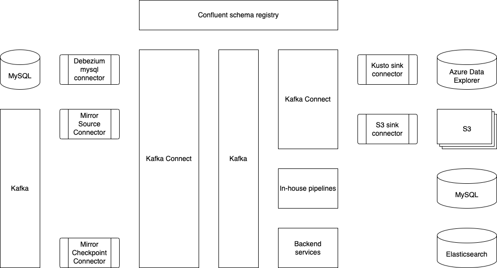
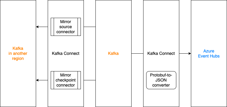
This is what Coban’s Kafka Connect stack looks like today. Multiple data sources and data sinks, such as MySQL, S3 and Azure Data Explorer, have already been supported and productionised.
The Coban team has been using Protobuf as the serialisation-deserialisation (SerDes) format in Kafka. Therefore, the role of Confluent schema registry (shown at the top of the figure) is crucial to the Kafka Connect ecosystem, as it serves as the building block for conversions such as Protobuf-to-Avro, Protobuf-to-JSON and Protobuf-to-Parquet.
What problems are we trying to solve?
Problem 1: Change Data Capture (CDC)
In a big organisation like Grab, we handle large volumes of data and changes across many services on a daily basis, so it is important for these changes to be reflected in real time.
In addition, there are other technical challenges to be addressed:
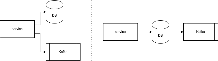
As shown in the figure below, data is written twice in the code base – once into the database (DB) and once as a message into Kafka. In order for the data in the DB and Kafka to be consistent, the two writes have to be atomic in a two-phase commit protocol (or other atomic commitment protocols), which is non-trivial and impacts availability.
Some use cases require data both before and after a change.
Problem 2: Message mirroring for disaster recovery
The Coban team has done some research on Kafka MirrorMaker, an open-source solution. While it can ensure better data consistency, it takes significant effort to adopt it onto existing Kubernetes infrastructure hosted by the Coban team and achieve high availability.
Another major challenge that the Coban team faces is offset mirroring and translation, which is a known challenge in Kafka communities. In order for Kafka consumers to seamlessly resume their work with a backup Kafka after a disaster, we need to cater for offset translation.
Data ingestion into Azure Event Hubs
Azure Event Hubs has a Kafka-compatible interface and natively supports JSON and Avro schema. The Coban team uses Protobuf as the SerDes framework, which is not supported by Azure Event Hubs. It means that conversions have to be done for message ingestion into Azure Event Hubs.
Solution
To tackle these problems, the Coban team has picked Kafka Connect because:
It is an open-source framework with a relatively big community that we can consult if we run into issues.
It has the ability to plug in transformations and custom conversion logic.
Let us see how Kafka Connect can be used to resolve the previously mentioned problems.
Kafka Connect with Debezium connectors
Debezium is a framework built for capturing data changes on top of Apache Kafka and the Kafka Connect framework. It provides a series of connectors for various databases, such as MySQL, MongoDB and Cassandra.
Here are the benefits of MySQL binlog streams:
They not only provide changes on data, but also give snapshots of data before and after a specific change.
Some producers no longer have to push a message to Kafka after writing a row to a MySQL database. With Debezium connectors, services can choose not to deal with Kafka and only handle MySQL data stores.
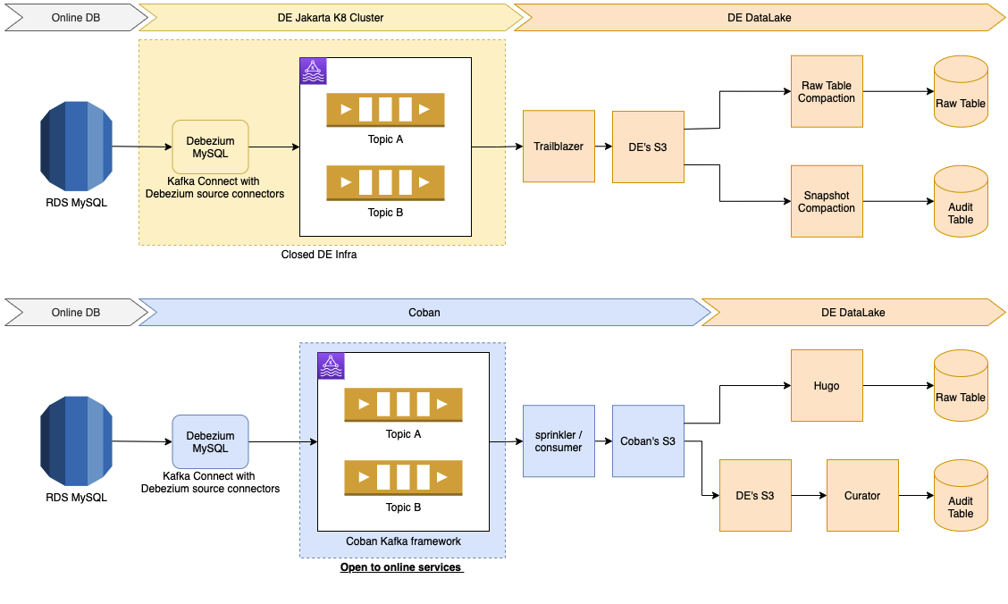
Architecture
In case of DB upgrades and outages
DB Data Definition Language (DDL) changes, migrations, splits and outages are common in database operations, and each operation type has a systematic resolution.
The Debezium connector has built-in features to handle DDL changes made by DB migration tools, such as pt-online-schema-change, which is used by the Grab DB Ops team.
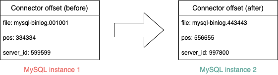
To deal with MySQL instance changes and database splits, the Coban team leverages on the Kafka Connect framework’s ability to change the offsets of connectors. By changing the offsets, Debezium connectors can properly function after DB migrations and resume binlog synchronisation from any position in any binlog file on a MySQL instance.
The CDC project on MySQL via Debezium connectors has been greatly successful in Grab. One of the biggest examples is its adoption in the Elasticsearch optimisation carried out by GrabFood, which has been published in another blog.
MirrorMaker2 with offset translation
Kafka MirrorMaker2 (MM2), developed in and shipped together with the Apache Kafka project, is a utility to mirror messages and consumer offsets. However, in the Coban team, the MM2 stack is deployed on the Kafka Connect framework per connector because:
A few Kafka Connect clusters have already been provisioned.
Compared to launching three connectors bundled in MM2, Coban can have finer controls on MirrorSourceConnector and MirrorCheckpointConnector, and manage both of them in an infrastructure-as-code way via Hashicorp Terraform.
Success stories
Ensuring business continuity is a key priority for Grab and this includes the ability to recover from incidents quickly. In 2021H2, there was a campaign that ran across many teams to examine the readiness and robustness of various services and middlewares. Coban’s Kafka is one of these services that proved to be robust after rounds of chaos engineering. With MM2 on Kafka Connect to mirror both messages and consumer offsets, critical services and pipelines could safely be replicated and launched across AWS regions if outages occur.
Because the Coban team has proven itself as the battle-tested Kafka service provider in Grab, other teams have also requested to migrate streams from self-managed Kafka clusters to ones managed by Coban. MM2 has been used in such migrations and brought zero downtime to the streams’ producers and consumers.
Mirror to Azure Event Hubs with an in-house converter
The Analytics team runs some real time ingestion and analytics projects on Azure. To support this cross-cloud use case, the Coban team has adopted MM2 for message mirroring to Azure Event Hubs.
Typically, Event Hubs only accept JSON and Avro bytes, which is incompatible with the existing SerDes framework. The Coban team has developed a custom converter that converts bytes serialised in Protobuf to JSON bytes at runtime.
These steps explain how the converter works:
Deserialise bytes in Kafka to a Protobuf DynamicMessage according to a schema retrieved from the Confluent™ schema registry.
Perform a recursive post-order depth-first-search on each field descriptor in the DynamicMessage.
Convert every Protobuf field descriptor to a JSON node.
Serialise the root JSON node to bytes.
The converter has not been open sourced yet.
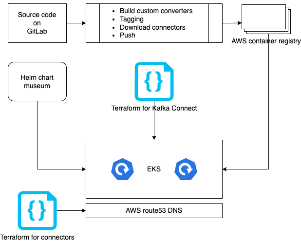
Deployment
Docker containers are the Coban team’s preferred infrastructure, especially since some production Kafka clusters are already deployed on Kubernetes. The long-term goal is to provide Kafka in a software-as-a-service (SaaS) model, which is why Kubernetes was picked. The diagram below illustrates how Kafka Connect clusters are built and deployed.
What’s next?
The Coban team is iterating on a unified control plane to manage resources like Kafka topics, clusters and Kafka Connect. In the foreseeable future, internal users should be able to provision Kafka Connect connectors via RESTful APIs and a graphical user interface (GUI).
At the same time, the Coban team is closely working with the Data Engineering team to make Kafka Connect the preferred tool in Grab for moving data in and out of external storages (S3 and Apache Hudi).
Coban is hiring!
The Coban (Real-time Data Platform) team at Grab in Singapore is hiring software and site reliability engineers at all levels as we double down on growing our platform capabilities.
Join us in building state-of-the-art, mission critical, TB/hour scale data platforms that enable thousands of engineers, data scientists, and analysts to serve millions of consumers, businesses, and partners across Southeast Asia!
Join us
Grab is a leading superapp in Southeast Asia, providing everyday services that matter to consumers. More than just a ride-hailing and food delivery app, Grab offers a wide range of on-demand services in the region, including mobility, food, package and grocery delivery services, mobile payments, and financial services across over 400 cities in eight countries.
Powered by technology and driven by heart, our mission is to drive Southeast Asia forward by creating economic empowerment for everyone. If this mission speaks to you, join our team today!
At Grab, we run large marketing campaigns every day. A typical campaign may require executing multiple actions for millions of users all at once. The actions may include sending rewards, awarding points, and sending messages. Here is what a campaign may look like: On 1st Jan 2022, send two ride rewards to all the users in the “heavy users” segment. Then, send them a congratulatory message informing them about the reward.
Years ago, Grab’s marketing team used to stay awake at midnight to manually trigger such campaigns. They would upload a file at 12 am and then wait for a long time for the campaign execution to complete. To solve this pain point and support more capabilities down this line, we developed a “batch job” service, which is part of our in-house real-time automation engine, Trident.
The following are some services we use to support Grab’s marketing teams:
Rewards: responsible for managing rewards.
Messaging: responsible for sending messages to users. For example, push notifications.
Segmentation: responsible for storing and retrieving segments of users based on certain criteria.
For simplicity, only the services above will be referenced for this article. The “batch job” service we built uses rewards and messaging services for executing actions, and uses the segmentation service for fetching users in a segment.
System requirements
Functional requirements
Apply a sequence of actions targeting a large segment of users at a scheduled time, display progress to the campaign manager and provide a final report.
For each user, the actions must be executed in sequence; the latter action can only be executed if the preceding action is successful.
Non-functional requirements
Quick execution and high turnover rate.
Definition of turnover rate: the number of scheduled jobs completed per unit time.
Maximise resource utilisation and balance server load.
For the sake of brevity, we will not cover the scheduling logic, nor the generation of the report. We will focus specifically on executing actions.
Naive approach
Let’s start thinking from the most naive solution, and improve from there to reach an optimised solution.
Here is the pseudocode of a naive action executor.
def executeActionOnSegment(segment, actions):
   for user in fetchUsersInSegment(segment):
       for action in actions:
           success := doAction(user, action)
           if not success:
               break
           recordActionResult(user, action)

def doAction(user, action):
   if action.type == "awardReward":
       rewardService.awardReward(user, action.meta)
   elif action.type == "sendMessage":
       messagingService.sendMessage(user, action.meta)
   else:
       # other action types ...
One may be able to quickly tell that the naive solution does not satisfy our non-functional requirements for the following reasons:
Execution is slow:
The programme is single-threaded.
Actions are executed for users one by one in sequence.
Each call to the rewards and messaging services will incur network trip time, which impacts time cost.
Resource utilisation is low: The actions will only be executed on one server. When we have a cluster of servers, the other servers will sit idle.
Here are our alternatives for fixing the above issues:
Actions for different users should be executed in parallel.
API calls to other services should be minimised.
Distribute the work of executing actions evenly among different servers.
Note: Actions for the same user have to be executed in sequence. For example, if a sequence of required actions are (1) award a reward, (2) send a message informing the user to use the reward, then we can only execute action (2) after action (1) is successfully done for logical reasons and to avoid user confusion.
Our approach
A message queue is a well-suited solution to distribute work among multiple servers. We selected Kafka, among numerous message services, due to its following characteristics:
High throughput: Kafka can accept reads and writes at a very high speed.
Robustness: Events in Kafka are distributedly stored with redundancy, without a need to worry about data loss.
Pull-based consumption: Consumers can consume events at their own speed. This helps to avoid overloading our servers.
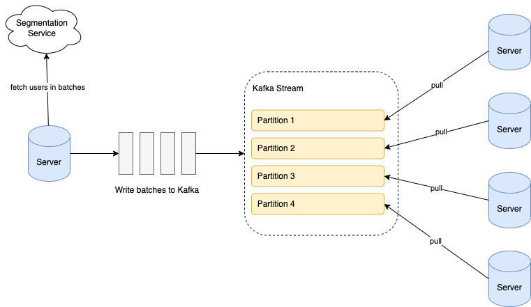
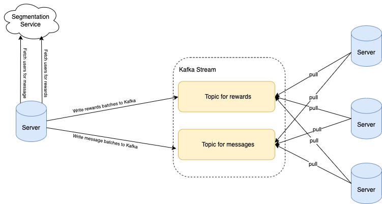
When a scheduled campaign is triggered, we retrieve the users from the segment in batches; each batch comprises around 100 users. We write the batches into a Kafka stream, and all our servers consume from the stream to execute the actions for the batches. The following diagram illustrates the overall flow.
Data in Kafka is stored in partitions. The partition configuration is important to ensure that the batches are evenly distributed among servers:
Number of partitions: Ensure that the number of stream partitions is greater than or equal to the max number of servers we will have in our cluster. This is because one Kafka partition can only be consumed by one consumer. If we have more consumers than partitions, some consumers will not receive any data.
Partition key: For each batch, assign a hash value as the partition key to randomly allocate batches into different partitions.
Now that work is distributed among servers in batches, we can consider how to process each batch faster. If we follow the naive logic, for each user in the batch, we need to call the rewards or messaging service to execute the actions. This will create very high QPS (queries per second) to those services, and incur significant network round trip time.
To solve this issue, we decided to build batch endpoints in rewards and messaging services. Each batch endpoint takes in a list of user IDs and action metadata as input parameters, and returns the action result for each user, regardless of success or failure. With that, our batch processing logic looks like the following:
In the implementation of batch endpoints, we also made optimisations to reduce latency. For example, when awarding rewards, we need to write the records of a reward being given to a user in multiple database tables. If we make separate DB queries for each user in the batch, it will cause high QPS to DB and incur high network time cost. Therefore, we grouped all the users in the batch into one DB query for each table update instead.
Benchmark tests show that using the batch DB query reduced API latency by up to 85%.
Further optimisations
As more campaigns started running in the system, we came across various bottlenecks. Here are the optimisations we implemented for some major examples.
Shard stream by action type
Two widely used actions are awarding rewards and sending messages to users. We came across situations where the sending of messages was blocked because a different campaign of awarding rewards had already started. If millions of users were targeted for rewards, this could result in significant waiting time before messages are sent, ultimately leading them to become irrelevant.
We found out the API latency of awarding rewards is significantly higher than sending messages. Hence, to make sure messages are not blocked by long-running awarding jobs, we created a dedicated Kafka topic for messages. By having different Kafka topics based on the action type, we were able to run different types of campaigns in parallel.
Shard stream by country
Grab operates in multiple countries. We came across situations where a campaign of awarding rewards to a small segment of users in one country was delayed by another campaign that targeted a huge segment of users in another country. The campaigns targeting a small set of users are usually more time-sensitive.
Similar to the above solution, we added different Kafka topics for each country to enable the processing of campaigns in different countries in parallel.
Remove unnecessary waiting
We observed that in the case of chained actions, messaging actions are generally the last action in the action list. For example, after awarding a reward, a congratulatory message would be sent to the user.
We realised that it was not necessary to wait for a sending message action to complete before processing the next batch of users. Moreover, the latency of the sending messages API is lower than awarding rewards. Hence, we adjusted the sending messages API to be asynchronous, so that the task of awarding rewards to the next batch of users can start while messages are being sent to the previous batch.
Conclusion
We have architected our batch jobs system in such a way so that it can be enhanced and optimised without redoing its work. For example, although we currently obtain the list of targeted users from a segmentation service, in the future, we may obtain this list from a different source, for example, all Grab Platinum tier members.
Join us
Grab is a leading superapp in Southeast Asia, providing everyday services that matter to consumers. More than just a ride-hailing and food delivery app, Grab offers a wide range of on-demand services in the region, including mobility, food, package and grocery delivery services, mobile payments, and financial services across over 400 cities in eight countries.
Powered by technology and driven by heart, our mission is to drive Southeast Asia forward by creating economic empowerment for everyone. If this mission speaks to you, join our team today!
In large organisations, it is a common practice to isolate the cloud resources of different verticals. Amazon Web Services (AWS) Virtual Private Cloud (VPC) is a convenient way of doing so. At Grab, while our core AWS services reside in a main VPC, a number of Grab Tech Families (TFs) have their own dedicated VPC. One such example is GrabKios. Previously known as “Kudo”, GrabKios was acquired by Grab in 2017 and has always been residing in its own AWS account and dedicated VPC.
In this article, we explore how we exposed an Apache Kafka cluster across multiple Availability Zones (AZs) in Grab’s main VPC, to producers and consumers residing in the GrabKios VPC, via a VPC Endpoint Service. This design is part of Coban unified stream processing platform at Grab.
There are several ways of enabling communication between applications across distinct VPCs; VPC peering is the most straightforward and affordable option. However, it potentially exposes the entire VPC networks to each other, needlessly increasing the attack surface.
Security has always been one of Grab’s top concerns and with Grab’s increasing growth, there is a need to deprecate VPC peering and shift to a method of only exposing services that require remote access. The AWS VPC Endpoint Service allows us to do exactly that for TCP/IPv4 communications within a single AWS region.
Setting up a VPC Endpoint Service compared to VPC peering is already relatively complex. On top of that, we need to expose an Apache Kafka cluster via such an endpoint, which comes with an extra challenge. Apache Kafka requires clients, called producers and consumers, to be able to deterministically establish a TCP connection to all brokers forming the cluster, not just any one of them.
Last but not least, we need a design that optimises performance and cost by limiting data transfer across AZs.
Note: All variable names, port numbers and other details used in this article are only used as examples.
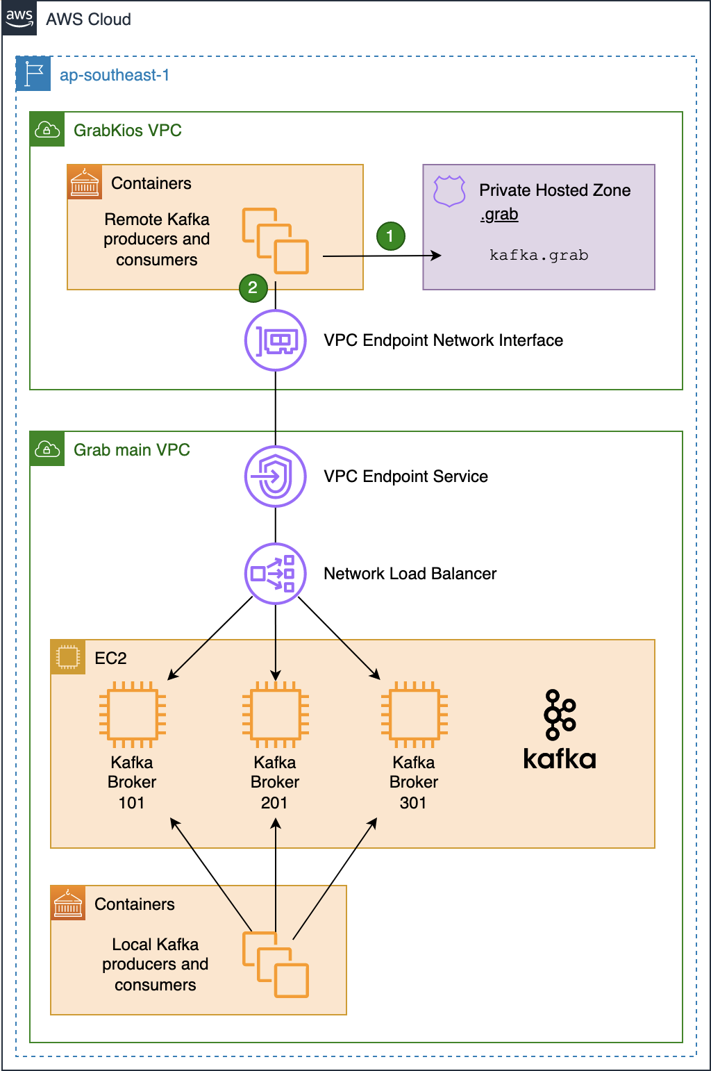
Architecture overview
As shown in this diagram, the Kafka cluster resides in the service provider VPC (Grab’s main VPC) while local Kafka producers and consumers reside in the service consumer VPC (GrabKios VPC).
In Grab’s main VPC, we created a Network Load Balancer (NLB) and set it up across all three AZs, enabling cross-zone load balancing. We then created a VPC Endpoint Service associated with that NLB.
Next, we created a VPC Endpoint Network Interface in the GrabKios VPC, also set up across all three AZs, and attached it to the remote VPC endpoint service in Grab’s main VPC. Apart from this, we also created a Route 53 Private Hosted Zone .grab and a CNAME record kafka.grab that points to the VPC Endpoint Network Interface hostname.
Lastly, we configured producers and consumers to use kafka.grab:10000 as their Kafka bootstrap server endpoint, 10000/tcp being an arbitrary port of our choosing. We will explain the significance of these in later sections.
Network Load Balancer setup
On the NLB in Grab’s main VPC, we set up the corresponding bootstrap listener on port 10000/tcp, associated with a target group containing all of the Kafka brokers forming the cluster. But this listener alone is not enough.
As mentioned earlier, Apache Kafka requires producers and consumers to be able to deterministically establish a TCP connection to all brokers. That’s why we created one listener for every broker in the cluster, incrementing the TCP port number for each new listener, so each broker endpoint would have the same name but with different port numbers, e.g. kafka.grab:10001 and kafka.grab:10002.
We then associated each listener with a dedicated target group containing only the targeted Kafka broker, so that remote producers and consumers could differentiate between the brokers by their TCP port number.
The following listeners and associated target groups were set up on the NLB:
In the Kafka brokers’ Security Group (SG), we added an ingress SG rule allowing 9094/tcp traffic from each of the three private IP addresses of the NLB. As mentioned earlier, the NLB was set up across all three AZs, with each having its own private IP address.
On the GrabKios VPC (consumer side), we created a new SG and attached it to the VPC Endpoint Network Interface. We also added ingress rules to allow all producers and consumers to connect to tcp/10000-10003.
Kafka setup
Kafka brokers typically come with a listener on port 9092/tcp, advertising the brokers by their private IP addresses. We kept that default listener so that local producers and consumers in Grab’s main VPC could still connect directly.
$ kcat -L -b 10.0.0.1:9092
 3 brokers:
 broker 101 at 10.0.0.1:9092 (controller)
 broker 201 at 10.0.0.2:9092
 broker 301 at 10.0.0.3:9092
... truncated output ...
We also configured all brokers with an additional listener on port 9094/tcp that advertises the brokers by:
Their shared private name kafka.grab.
Their distinct TCP ports previously set up on the NLB’s dedicated listeners.
$ kcat -L -b 10.0.0.1:9094
 3 brokers:
 broker 101 at kafka.grab:10001 (controller)
 broker 201 at kafka.grab:10002
 broker 301 at kafka.grab:10003
... truncated output ...
Note that there is a difference in how the broker’s endpoints are advertised in the two outputs above. The latter enables connection to any particular broker from the GrabKios VPC via the VPC Endpoint Service.
It would definitely be possible to advertise the brokers directly with the remote VPC Endpoint Interface hostname instead of kafka.grab, but relying on such a private name presents at least two advantages.
First, it decouples the Kafka deployment in the service provider VPC from the infrastructure deployment in the service consumer VPC. Second, it makes the Kafka cluster easier to expose to other remote VPCs, should we need it in the future.
Limiting data transfer across Availability Zones
At this stage of the setup, our Kafka cluster is fully reachable from producers and consumers in the GrabKios VPC. Yet, the design is not optimal.
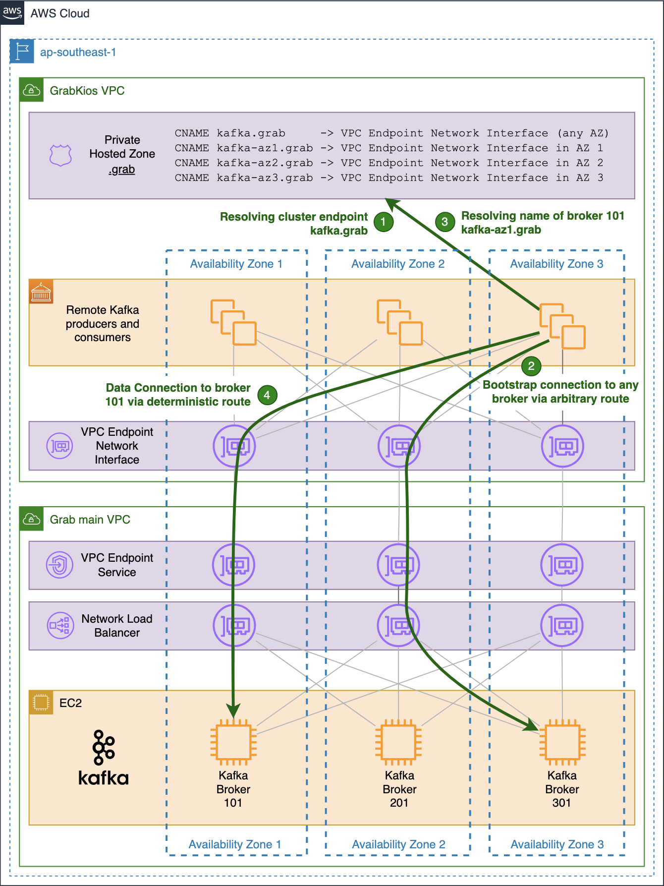
When a producer or a consumer in the GrabKios VPC needs to connect to a particular broker, it uses its individual endpoint made up of the shared name kafka.grab and the broker’s dedicated TCP port.
The shared name arbitrarily resolves into one of the three IP addresses of the VPC Endpoint Network Interface, one for each AZ.
Hence, there is a fair chance that the obtained IP address is neither in the client’s AZ nor in that of the target Kafka broker. The probability of this happening can be as high as 2/3 when both client and broker reside in the same AZ and 1/3 when they do not.
While that is of little concern for the initial bootstrap connection, it becomes a serious drawback for actual data transfer, impacting the performance and incurring unnecessary data transfer cost.
For this reason, we created three additional CNAME records in the Private Hosted Zone in the GrabKios VPC, one for each AZ, with each pointing to the VPC Endpoint Network Interface zonal hostname in the corresponding AZ:
kafka-az1.grab
kafka-az2.grab
kafka-az3.grab
Note that we used az1, az2, az3 instead of the typical AWS 1a, 1b, 1c suffixes, because the latter’s mapping is not consistent across AWS accounts.
We also reconfigured each Kafka broker in Grab’s main VPC by setting their 9094/tcp listener to advertise brokers by their new zonal private names.
$ kcat -L -b 10.0.0.1:9094
 3 brokers:
 broker 101 at kafka-az1.grab:10001 (controller)
 broker 201 at kafka-az2.grab:10002
 broker 301 at kafka-az3.grab:10003
... truncated output ...
Our private zonal names are shared by all brokers in the same AZ while TCP ports remain distinct for each broker. However, this is not clearly shown in the output above because our cluster only counts three brokers, one in each AZ.
The previous common name kafka.grab remains in the GrabKios VPC’s Private Hosted Zone and allows connections to any broker via an arbitrary, likely non-optimal route. GrabKios VPC producers and consumers still use that highly-available endpoint to initiate bootstrap connections to the cluster.
Future improvements
For this setup, scalability is our main challenge. If we add a new broker to this Kafka cluster, we would need to:
Assign a new TCP port number to it.
Set up a new dedicated listener on that TCP port on the NLB.
Configure the newly spun up Kafka broker to advertise its service with the same TCP port number and the private zonal name corresponding to its AZ.
Add the new broker to the target group of the bootstrap listener on the NLB.
Update the network SG rules on the service consumer side to allow connections to the newly allocated TCP port.
We rely on Terraform to dynamically deploy all AWS infrastructure and on Jenkins and Ansible to deploy and configure Apache Kafka. There is limited overhead but there are still a few manual actions due to a lack of integration. These include transferring newly allocated TCP ports and their corresponding EC2 instances’ IP addresses to our Ansible inventory, commit them to our codebase and trigger a Jenkins job deploying the new Kafka broker.
Another concern of this setup is that it is only applicable for AWS. As we are aiming to be multi-cloud, we may need to port it to Microsoft Azure and leverage the Azure Private Link service.
In both cases, running Kafka on Kubernetes with the Strimzi operator would be helpful in addressing the scalability challenge and reducing our adherence to one particular cloud provider. We will explain how this solution has helped us address these challenges in a future article.
Special thanks to David Virgil Naranjo whose blog post inspired this work.
Join us
Grab is a leading superapp in Southeast Asia, providing everyday services that matter to consumers. More than just a ride-hailing and food delivery app, Grab offers a wide range of on-demand services in the region, including mobility, food, package and grocery delivery services, mobile payments, and financial services across over 400 cities in eight countries.
Powered by technology and driven by heart, our mission is to drive Southeast Asia forward by creating economic empowerment for everyone. If this mission speaks to you, join our team today!
Using analytics to gain insights from a variety of datasets is key to successful transformation. There are many options to consider to realize the full value and potential of our data in a hybrid cloud infrastructure. Common practice is to route data produced from on-premises to a central repository or data lake. Here it can be consumed by multiple applications.
You can use an Apache Kafka cluster for data movement from on-premises to the data lake, using Amazon Simple Storage Service (Amazon S3). But you must either replicate the topics onto a cloud cluster, or develop a custom connector to read and copy the topics to Amazon S3. This presents a challenge for many customers.
This blog presents another option; an architecture solution leveraging AWS Glue.
Kafka and ETL processing
Apache Kafka is an open-source distributed event streaming platform used by thousands of companies for high-performance data pipelines, streaming analytics, data integration, and mission-critical applications. You can use Kafka clusters as a system to move data between systems. Producers typically publish data (or push) to a Kafka topic, where an application can consume it. Consumers are usually custom applications that feed data into respective target applications. These targets can be a data warehouse, an Amazon OpenSearch Service cluster, or others.
AWS Glue offers the ability to create jobs that will extract, transform, and load (ETL) data. This allows you to consume from many sources, such as from Apache Kafka, Amazon Kinesis Data Streams, or Amazon Managed Streaming for Apache Kafka (Amazon MSK). The jobs cleanse and transform the data, and then load the results into Amazon S3 data lakes or JDBC data stores.
Hybrid solution and architecture design
In most cases, the first step in building a responsive and manageable architecture is to review the data itself. For example, if we are processing insurance policy data from a financial organization, our data may contain fields that identify customer data. These can be account ID, an insurance claim identifier, and the dollar amount of the specific claim. Glue provides the ability to change any of these field types into the expected data lake schema type for processing.
Figure 1. Data flow – Source to data lake target
Next, AWS Glue must be configured to connect to the on-premises Kafka server (see Figure 1). Private and secure connectivity to the on-premises environment can be established via AWS Direct Connect or a VPN solution. Traffic from the Amazon Virtual Private Cloud (Amazon VPC) is allowed to access the cluster directly. You can do this by creating a three-step streaming ETL job:
Create a Glue connection to the on-premises Kafka source
Create a Data Catalog table
Create an ETL job, which saves to an S3 data lake
Configuring AWS Glue
Create a connection. Using AWS Glue, create a secure SSL connection in the Data Catalog using the predefined Kafka connection type. Enter the hostname of the on-premises cluster and use the custom-managed certificate option for additional security. If you are in a development environment, you are required to generate a self-signed SSL certificate. Use your Kafka SSL endpoint to connect to Glue. (AWS Glue also supports client authentication for Apache Kafka streams.)
Specify a security group. To allow AWS Glue to communicate between its components, specify a security group with a self-referencing inbound rule for all TCP ports. By creating this rule, you can restrict the source to the same security group in the Amazon VPC. Ensure you check the default security group for your VPC, as it could have a preconfigured self-referencing inbound rule for ALL traffic.
Create the Data Catalog. Glue can auto-create the data schema. Since it’s a simple flat file, use the schema detection function of Glue. Set up the Kafka topic and refer to the connection.
Define the job properties. Create the AWS Identity and Access Management (IAM) role to allow Glue to connect to S3 data. Select an S3 bucket and format. In this case, we use CSV and enable schema detection.
The Glue job can be scheduled, initiated manually, or by using an event driven architecture. Note that Glue does not yet support the “test connection” option within the console. Make sure you set the “Job Timeout” and enter a duration in minutes because the default value is blank.
When the job runs, it pulls the latest topics from the source on-premises Kafka cluster. Glue supports checkpoints to ensure that all source data is processed. By default, AWS Glue processes and writes out data in 100-second windows. This allows data to be processed efficiently and permits aggregations to be performed on data arriving later. You can modify this window size to increase timeliness or aggregation accuracy. AWS Glue streaming jobs use checkpoints rather than job bookmarks to track the data that has been read. AWS Glue bills hourly for streaming ETL jobs only while they are running.
Now that the connection is complete and the job is created, we can format the source data needed for the data lake. AWS Glue offers a set of built-in transforms that you can use to process your data using your ETL script. The transformed data is then placed in S3, where it can be leveraged as part of a larger data lake environment.
Many additional steps can be taken to render even more value from the information. For example, one team may choose to use a business intelligence tool like Amazon QuickSight to visualize and embed the data into an internal dashboard. Another team may want to use event driven architectures to notify financial analysts and initiate downstream actions when specific types of data are discovered. There are endless opportunities that should be determined by the business needs.
Summary
In this blog post, we have given an overview of an architecture that provides hybrid cloud data integration and analytics capability. Once the data is transformed and hosted in the S3 data lake, we can provide secure, reliable access to gain valuable insights. This solution allows for a variety of different producers and consumers, with the ability to handle increasing volumes of data.
AWS Glue along with Apache Kafka will ensure that your on-premises workloads are tightly integrated with your larger data lake solution.
If you have questions, post your thoughts in the comments section.
At Netflix, hundreds of different device types, from streaming sticks to smart TVs, are tested every day through automation to ensure that new software releases continue to deliver the quality of the Netflix experience that our customers enjoy. In addition, Netflix continuously works with its partners (such as Roku, Samsung, LG, Amazon) to port the Netflix SDK to their new and upcoming devices (TVs, smart boxes, etc), to ensure the quality bar is reached before allowing the Netflix application on the device to go out into the world. The Partner Infrastructure team at Netflix provides solutions to support these two significant efforts by enabling device management at scale.
Background
To normalize the diversity of networking environments across both the Netflix and Partner networks and create a consistent and controllable computing environment on which users can run regression and Netflix application certification testing for devices, the Partner Infrastructure team provides a customized embedded computer called the Reference Automation Environment (RAE). Complementing the hardware is the software on the RAE and in the cloud, and bridging the software on both ends is a bi-directional control plane. Together, they form the Device Management Platform, which is the infrastructural foundation for Netflix Test Studio (NTS). Users then effectively run tests by connecting their devices to the RAE in a plug-and-play fashion.
The platform allows for effective device management at scale, and its feature set is broadly divided into two areas:
Provide a service-level abstraction for controlling devices and their environments (hardware and software topologies).
Collect and aggregate information and state updates for all devices attached to the RAEs in the fleet. In this blog post, we will focus on the latter feature set.
Over the lifecycle of a device connected to the RAE, the device can change attributes at any time. For example, when running tests, the state of the device will change from “available for testing” to “in test.” In addition, because many of these devices are pre-production devices and thus subject to frequent firmware changes, attributes that are generally static in production devices can sometimes change as well, such as the MAC address and the Electronic Serial Number (ESN) assigned to the Netflix installation on the device. As such, it is very critical to be able to keep device information up to date for device tests to work properly. In the Device Management Platform, this is achieved by having device updates be event-sourced through the control plane to the cloud so that NTS will always have the most up-to-date information about the devices available for testing. The challenge, then, is to be able to ingest and process these events in a scalable manner, i.e., scaling with the number of devices, which will be the focus of this blog post.
System Setup
Architecture
The following diagram summarizes the architecture description:
Figure 1: Event-sourcing architecture of the Device Management Platform.
The RAE is configured to be effectively a router that devices under test (DUTs) are connected to. On the RAE, there exists a service called the Local Registry, which is responsible for detecting, onboarding, and maintaining information about all devices connected to the LAN side of the RAE. When a new hardware device is connected, the Local Registry detects and collects a set of information about it, such as networking information and ESN. At periodic intervals, the Local Registry probes the device to check on its connection status. As the device attributes and properties change over time, these changes are saved into the Local Registry and simultaneously published upstream to the Device Management Platform’s control plane. In addition to attribute changes, a complete snapshot of the device record is published upstream by the Local Registry at regular intervals as a form of state reconciliation. These checkpoint events enable faster state reconstruction by consumers of the data feed while guarding against missed updates.
On the cloud side, a service called the Cloud Registry ingests the device information updates published by the Local Registry instance, processes them, and subsequently pushes materialized data into a datastore backed by CockroachDB. CockroachDB is chosen as the backing data store since it offered SQL capabilities, and our data model for the device records was normalized. In addition, unlike other SQL stores, CockroachDB is designed from the ground up to be horizontally scalable, which addresses our concerns about Cloud Registry’s ability to scale up with the number of devices onboarded onto the Device Management Platform.
Control Plane
MQTT forms the basis of the control plane for the Device Management Platform. MQTT is an OASIS standard messaging protocol for the Internet of Things (IoT) and was designed as a highly lightweight yet reliable publish/subscribe messaging transport that is ideal for connecting remote devices with a small code footprint and minimal network bandwidth. MQTT clients connect to the MQTT broker and send messages prefixed with a topic. In contrast, the broker is responsible for receiving all messages, filtering them, determining who is subscribed to which topic, and sending the messages to the subscribed clients accordingly. The key features that make MQTT highly appealing to us are its support for hierarchical topics, client authentication and authorization, per-topic ACLs, and bi-directional request/response message patterns, all of which are crucial for the business use cases we have for the control plane.
Inside the control plane, device commands and device information updates are prefixed with a topic string that includes both the RAE serial number and the device_session_id, which is a UUID corresponding to a device session. Embedding these two bits of information into the topic for every message allows for us to apply topic ACLs and effectively control which RAEs and DUTs users can see and interact with, in the safety and isolation against other users’ devices.
Since Kafka is a supported messaging platform at Netflix, a bridge is established between the two protocols to allow cloud-side services to communicate with the control plane. Through the bridge, MQTT messages are converted directly to Kafka records, where the record key is set to be the MQTT topic that the message was assigned to. Since device information updates published on MQTT contain the device_session_id in the topic, this means that all device information updates for a given device session will effectively appear on the same Kafka partition, thus giving us a well-defined message order for consumption.
Canary Test Workloads
In addition to serving the regular message traffic between users and DUTs, the control plane itself is stress-tested at roughly 3-hour intervals, where nearly 3000 ephemeral MQTT clients are created to connect to and generate flash traffic on the MQTT brokers. This is intended to be a canary test to verify that the brokers are online and able to handle sudden influxes of client connections and high message loads. As such, we can see that the traffic load on the Device Management Platform’s control plane is very dynamic over time.
Adherence to the Paved-Path
At Netflix, we emphasize building out solutions that use paved-path tooling as much as possible (see posts here and here). In particular, the flavor of Spring Boot Native maintained by the Runtime team is the basis for many of the web services developed inside Netflix (including the Cloud Registry). The Netflix Spring package comes with all the integrations needed for applications to work seamlessly within the Netflix ecosystem. In particular, the Kafka integration is the most relevant for this blog post.
Translating to System Requirements
Given the system setup that we have described, we came up with a list of fundamental business requirements that the Cloud Registry’s Kafka-based device updates processing solution must address.
Back-Pressure Support
Because the processing workload varies significantly over time, the solution must first and foremost scale with the message load by providing back-pressure support as defined in the Reactive Streams specification — in other words, the solution should be able to switch between push and pull-based back-pressure models depending on the downstream being able to cope with the message production rate or not.
In-Order Processing
The semantics of correct device information updates ingestion requires that messages be consumed in the order that they are produced. Since message order is guaranteed per Kafka partition, and all updates for a given device session are assigned to the same partition, this means that the order of processing of updates for each device can be enforced as long as only one thread is assigned per partition. At the same time, events arriving on different partitions should be processed in parallel for maximum throughput.
Fault Tolerance
If the underlying KafkaConsumer crashes due to ephemeral system or network events, it should be automatically restarted. If an exception is thrown during the consumption of a message, the exception should be gracefully caught, and message consumption should seamlessly continue after the offending message is dropped.
Graceful Shutdown
Application shutdowns are necessary and inevitable when a service is re-deployed, or its instance group is resized. As such, processor shutdowns should be invokable from outside of the Kafka consumption context to facilitate graceful application termination. In addition, since Kafka messages are usually pulled down in batches by the KafkaConsumer, the implemented solution should, upon receiving the shutdown signal, consume and drain all the already-fetched messages remaining in its internal queue prior to shutting down.
Paved-Path Integration
As mentioned earlier, Spring is heavily employed as the paved-path solution for developing services at Netflix, and the Cloud Registry is a Spring Boot Native application. Thus, the implemented solution must integrate with Netflix Spring facilities for authentication and metrics support at the very minimum — the former for access to the Kafka clusters and the latter for service monitoring and alerts. In addition, the lifecycle management of the implemented solution must also be integrated into Spring’s lifecycle management.
Long-Term Maintainability
The implemented solution must be friendly enough for long-term maintenance support. This means that it must at the very least be unit- and functional-testable for rapid and iterative feedback-driven development, and the code must be reasonably ergonomic to lower the learning curve for new maintainers.
Adopting a Stream Processing Framework
There are many frameworks available for reliable stream processing for integration into web services (for example, Kafka Streams, Spring KafkaListener, Project Reactor, Flink, Alpakka-Kafka, to name a few). We chose Alpakka-Kafka as the basis of the Kafka processing solution for the following reasons.
Alpakka-Kafka turns out to satisfy all of the system requirements we laid out, including the need for Netflix Spring integration. It further provides advanced and fine-grained control over stream processing, including automatic back-pressure support and streams supervision.
Compared to the other solutions that may satisfy all of our system requirements, Akka is a much more lightweight framework, with its integration into a Spring Boot application being relatively short and concise. In addition, Akka and Alpakka-Kafka code is much less terse than the other solutions out there, which lowers the learning curve for maintainers.
The maintenance costs over time for an Alpakka-Kafka-based solution is much lower than that for the other solutions, as both Akka and Alpakka-Kafka are mature ecosystems in terms of documentation and community support, having been around for at least 12 and 6 years, respectively.
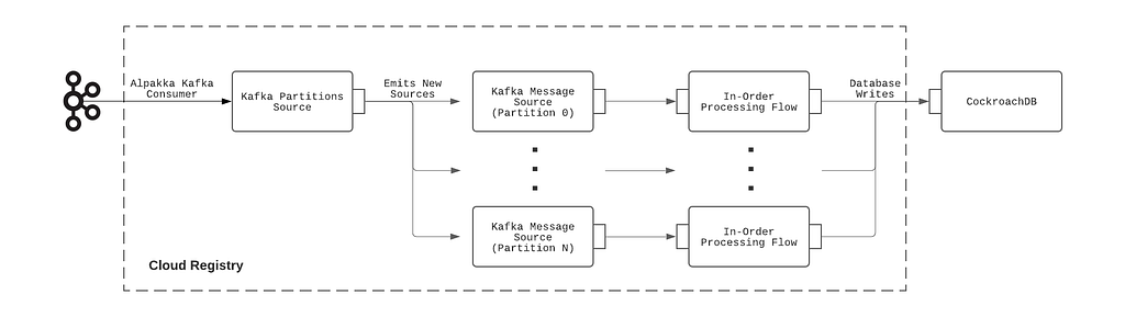
The construction of the Alpakka-based Kafka processing pipeline can be summarized with the following diagram:
Figure 2: Kafka processing pipeline employed by the Cloud Registry.
Implementation
The integration of Alpakka-Kafka streams with the Netflix Spring application context is very straightforward and is implemented as follows:
Import the Alpakka-Kafka library in build.gradle, butexclude the kafka-client transitive dependency that comes packaged with it so that the Netflix internal-enhanced variant is used.
Build a Spring @Configuration class that autowires the KafkaProperties bean injected by the Netflix Spring runtime and, using the Kafka settings available from that bean, construct an Alpakka-Kafka ConsumerSettings bean.
Construct an Alpakka-Kafka processing graph using the ConsumerSettings bean as an input.
Because this integration explicitly uses the Netflix-enhanced KafkaConsumer and Netflix Spring-injected Kafka settings, the authentication, and metrics-logging facilities that come with the paved-path Spring KafkaListener are immediately enjoyed by the Alpakka-Kafka-based solution.
Testing
Functional testing of the Alpakka-Kafka consumers is very straightforward with the EmbeddedKafka library, which provides an in-memory Kafka instance to run tests against. To scale up testing with the complexity of the Kafka message processing pipeline, the message processing code was separated from the Alpakka-Kafka graph code. This allowed the message processing code to be tested separately using functional tests while minimizing the surface area of required testing by EmbeddedKafka-based Kafka integration tests.
Results
Prior to Alpakka-Kafka
The original Kafka processing solution implemented in the Cloud Registry was built on Spring KafkaListener, primarily due to its immediate availability as a paved-path solution provided by Netflix Spring. A timeline of the transition from Spring KafkaListener to Alpakka-Kafka is presented here for a better understanding of the motivations for the transition.
Memory and GC Troubles
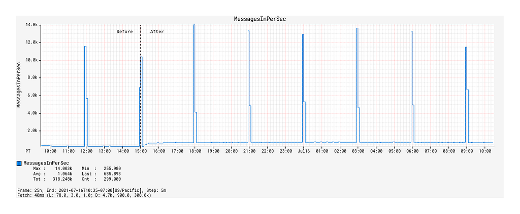
The Spring KafkaListener-based solution was deployed earlier this year, during which messages on the Kafka topic were sparse because the Local Registry was not fully in production at the time. Upstream event sourcing was fully enabled on the producer side at around 2021–07–15 15:00 PST. By the following morning, alerts were received regarding high memory consumption and GC latencies, to the point where the service was unresponsive to HTTP requests. An investigation of the JVM memory dump revealed an internal Kafka message concurrent queue whose size had grown uncontrollably to over 1.3 million elements.
The cause for this abnormal queue growth is due to Spring KafkaListener’s lack of native back-pressure support. With KafkaListener, the Kafka message fetch rate is fixed on application startup. However, it can be adjusted by tuning the max-poll-interval-ms and max-poll-records configuration values, which need to be somehow determined empirically beforehand for best performance. This setup is neither optimal nor break-proof since the Kafka message processing rate will vary depending on environmental factors, such as database latencies in our system setup. As a result, the KafkaListener ends up effectively over-consuming messages over time, which is manifested in the growth of its internal message queue.
After doubling the number of service instances and increasing the instance sizes with only mediocre success, the decision was made to look into an alternative Kafka processing solution with full back-pressure management capabilities.
Kafka Topic Metrics
The enabling of event-sourcing from Local Registry significantly increased the Device Management Platform’s control plane traffic, as evidenced by the 9x growth of Kafka topic message publication frequency from 100 messages / 90 kB incoming per second to 900 messages / 840kB incoming per second (Figure 3).
Figure 3: Message traffic over time before and after event-sourcing was enabled.
The spikes that occur on 3-hour intervals shown here correspond to the canary runs mentioned earlier that effectively load-test the Kafka topic with a flood of new records. Hereafter, they will be referred to as burst events. While the average message publication rate is low compared to the data systems out there that produce hundreds of thousands, if not millions, events per second, it does highlight the significance of having back-pressure management in place even at the lower end of the message load spectrum.
Kafka Consumption Improvements with Alpakka-Kafka
We now compare the Kafka consumption between the Spring KafkaListener-based Kafka processing solution and the Alpakka-Kafka-based solution, the latter of which was deployed to production on 2021–07–23 18:00 PST. In particular, we will look at three indicators of Kafka consumption performance: the message fetch rate, the max consumer lag, and the commit rate.
Fetch Request Metrics
Upon deployment of the Alpakka-Kafka-based processor, we made a few observations:
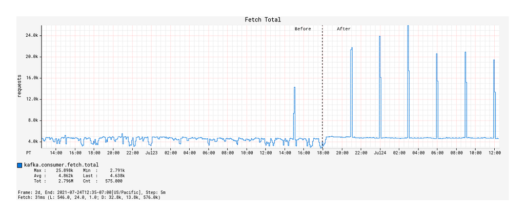
Prior to the deployment, the number of fetch calls over time generally remained unchanged across burst events but was otherwise actually quite unstable over time (Figure 4).
After the deployment, the fetch calls over time followed a 1:1 correspondence with the Kafka topic’s message publication rate, including the interval burst events (Figure 4). Outside of the burst event windows, the number of fetch calls over time was very stable.
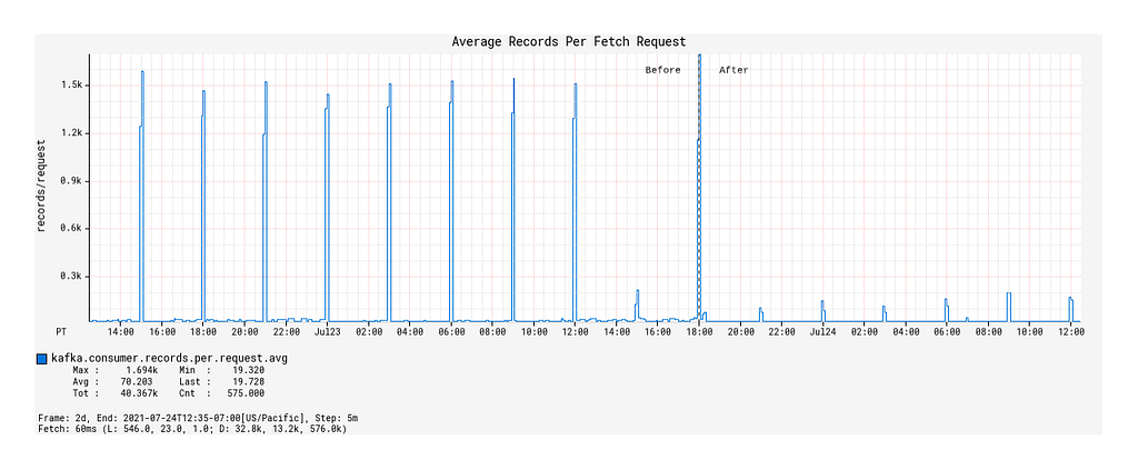
Surprisingly, the average number of records fetched per fetch request during the burst events windows decreased compared to that of the Spring KafkaListener-based processor (Figure 5).
What we can infer from these observations is that, with native back-pressure support in place, the Alpakka-Kafka-based processor is able to dynamically scale its Kafka consumption such that it is never under-consuming or over-consuming Kafka messages. This behavior keeps the processor constantly busy enough, but without overloading it with a growing queue of messages pulled from Kafka that eventually overflows the JVM’s memory and GC capacity.
Figure 4: Record fetch calls made by the KafkaConsumer over time, before and after deployment of the Alpakka-Kafka-based processor.Figure 5: Average number of records fetched per fetch request over time, before and after deployment.
Max Consumer Lag
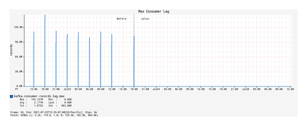
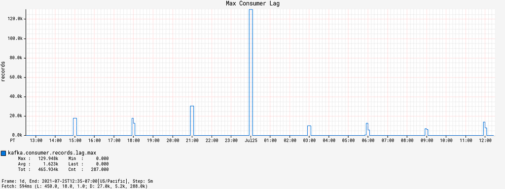
Except for JVM and service uptime, the most significant improvements with the Alpakka-Kafka-based processor manifested in the Kafka consumer lag metrics. While the Spring KafkaListener was deployed, the max consumer lag generally floated long-term at around 60,000 records, excluding the burst event time windows (this is not visually discernible from the graph due to the orders of magnitude differences in plotted values). From a functional point of view, this was unacceptable, as such a large constant lag value implies that device information updates will take a significantly long enough time to propagate into service such that it will be noticeable by our users. The situation exacerbates during the burst event windows, where the max consumer lag would increase to values of over 100 million records (Figure 6).
Since the deployment of the Alpakka-Kafka-based processor, the max consumer lag over time has averaged at zero outside of the burst event windows. Inside the burst event windows, the max consumer lag increases ephemerally to roughly 20,000 records, with only one outlier in the 48 hour time period since deployment (Figure 7). These metrics show us that the Kafka consumption patterns employed by Alpakka-Kafka and the streaming capabilities of Akka, in general, perform exceptionally well at scale, from the quiet use case to the presence of sudden huge message loads.
Figure 6: Max consumer lag of the KafkaConsumer over time, before and after deployment.Figure 7: Max consumer lag of the KafkaConsumer over time, magnified to the time window some time after deployment.
Commit Rate and Average Commit Latency
When a Kafka consumer fetches records, it can perform manual or automatic offset commits — this is configurable through enable.auto.commit. Contrary to the name, the semantics of manual vs auto commit don’t necessarily refer to how the offset commits are performed, but when in relations to the record fetch-process cycle. With auto commits, messages are acknowledged to have been received as soon as they are fetched and irrespective of processing, whereas with manual commits, the consumer can decide to acknowledge only after a message is properly processed.
By default, when enable.auto.commit is set to false, the Spring KafkaListener performs an offset commit every time a record is processed, i.e., the acknowledgement mode is set to AckMode.RECORD. This is exceedingly inefficient, and is known to reduce the message consumption throughput of the consumer. With the Alpakka-Kafka-based processor, we opted for making record commits in batches (set to 1000 by default), with a max interval of 1 second allowed between commits. This behavior is similar to the AckMode.COUNT_TIME acknowledgement mode in Spring KafkaListener, but with the added benefit of automatically attempting to complete outstanding commit requests when the Kafka consumption fails or terminates.
Under a manual offset commit scheme, it is always possible to re-process Kafka messages in the case of failures. To retain the (mainly) exactly-once processing that is guaranteed by the automatic offset commit scheme, the Kafka processor was updated to store device updates using idempotent upserts, i.e., perform an upsert conditioned on the timestamp of record in the database being earlier than the timestamp of the update to be upserted. This effectively ensures exactly-once processing on a per-event basis.
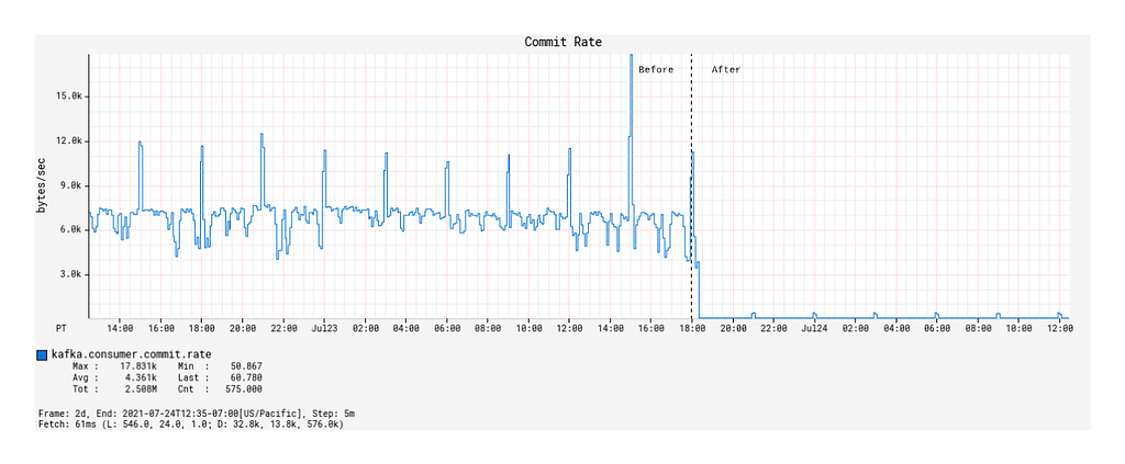
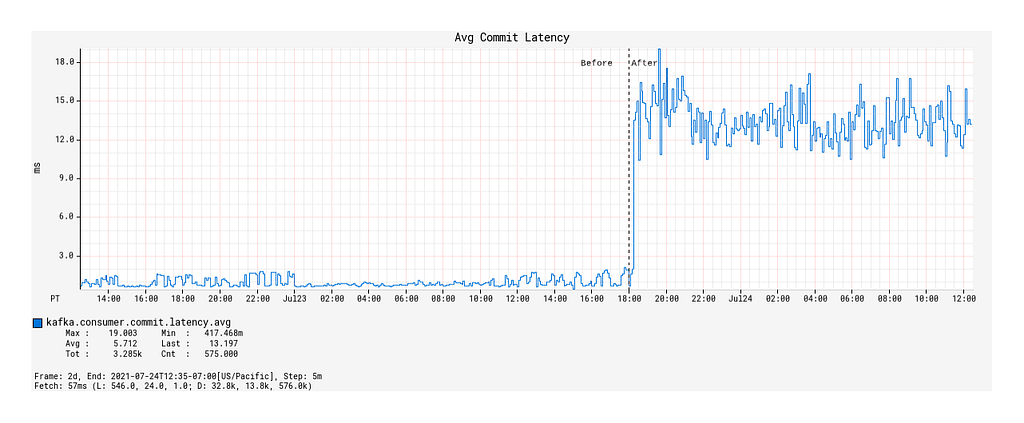
With the deployment of the Alpakka-Kafka-based processor, the commit rate was significantly lowered from roughly 7 kbytes/sec to 50 bytes/sec (Figure 8), but the average commit latency increased from 1 ms on average to 12 ms (Figure 9). Nonetheless, this is a considerable reduction in the network overhead spent on committing offsets, and has contributed significantly to the improved throughput of the Kafka processing.
Figure 8: Rate of offset commits made by the KafkaConsumer over time, before and after deployment.Figure 9: Average latency per offset commit over time, before and after deployment.
Conclusion
Kafka streams processing can be difficult to get right. Many system implementation details need to be considered in light of the business requirements. Fortunately, the primitives provided by Akka streams and Alpakka-Kafka empower us to achieve exactly this by allowing us to build streaming solutions that match the business workflows we have while scaling up developer productivity in building out and maintaining these solutions. With the Alpakka-Kafka-based processor in place in the Cloud Registry, we have ensured fault tolerance in the consumer side of the control plane, which is key to enabling accurate and reliable device state aggregation within the Device Management Platform.
Though we have achieved fault-tolerant message consumption, it is only one aspect of the design and implementation of the Device Management Platform. The reliability of the platform and its control plane rests on significant work made in several areas, including the MQTT transport, authentication and authorization, and systems monitoring, all of which we plan to discuss in detail in future blog posts. In the meantime, as a result of this work, we can expect the Device Management Platform to continue to scale to increasing workloads over time as we onboard ever more devices into our systems.
In this post, we will talk about the low-level discovery of Kafka connectors and tasks. When a Kafka task fails, a trigger is fired, which starts a remote command to restart the failed Kafka task. Of course, with the necessary logging around it.
You can find the template and scripts on the Zabbix share. But first, let’s talk a little bit about Kafka producers and consumers. Let’s say you have got a couple of connectors set up, pulling data from Postgres with Debezium and streaming it into Elasticsearch. The Postgres source is a bit flaky and goes offline periodically. If you view the status of the Postgres source, the producer, you noticed the task is failed. Kafka does not restart the failed task out of the box. We don’t wait for the customer to complain, but we let Zabbix actively monitor the tasks. A failed connector task is easy to restart using the Rest API. But manually restarting and watching a task is annoying. We used to do that at our business. Now Zabbix comes into play and restarts the failed Kafka task automatically. And we do sleep well.
About Kafka
Apache Kafka is a community distributed event streaming platform capable of handling trillions of events a day. Initially conceived as a messaging queue, Kafka is based on an abstraction of a distributed commit log. Since being created and open-sourced by LinkedIn in 2011, Kafka has quickly evolved from messaging queue to a full-fledged event streaming platform.
First, let’s do a curl and check the failed connector task.
So this is where the fun starts – we have a connector task with id “1” which has failed. At the end of the blog, Zabbix restarts the connector, but first, let’s look at an example. This curl post should restart the connector task: connect2.test.com id:1
curl -X POST http://localhost:8083/connectors/connect2.test.com/tasks/1/restart
Low-level discovery
The zabbix_kafka_connector template does work out of the box. To implemented the use cases provided in this blog you will need the scripts bundled together with the template. Kafka connectors can have multiple tasks. First, we determine the connectors and later the state of the connectors and tasks. Let’s run the following script – api_connectors.sh. I suggest you execute the script via a cronjob every 5 minutes, depending on your priority to run the curl jobs.
It creates two files, check_connectors, and get_connectors. Needless to say, we use curl with authentication in the production environment.
The next shell script get_connector_data.sh uses check_connectors and get_connectors files as input. It defines the connector {#CONNECTOR} and the connector tasks {#CONNECTOR_ID} with the corresponding ID used by low-level discovery. Down the line it might be more efficient to rewrite it as a python script. Json query is our useful friend here. The script is used by a user parameter later on.
get_connector_data.sh
#!/bin/sh
CONNECTOR=$(cat get_connectors)
CONNECTOR_IDS=$(cat get_connectors | tr -d ")
FIRST="1"
#create zabbix lld discovery connectors
echo "{"
echo " "data":["
for i in $CONNECTOR
do
if [ "$FIRST" -eq 0 ]
then
printf ",n"
fi
FIRST="0"
printf " {"{#CONNECTOR}": $i}"
done
#create zabbix lld discovery task connectors
for i in $CONNECTOR_IDS
do
IDS=$(cat check_connectors | jq --arg i ${i} -r '."'${i}'"| .status.tasks[].id')
for z in $IDS
do
if [ "$FIRST" -eq 0 ]
then
printf ",n"
fi
FIRST="0"
printf " {"{#CONNECTOR_ID}": "${i}-${z}"}"
done
done
#
printf "n ] n}"
Part of the script output will look like this, depending, of course, how many connectors there are and tasks in your Kafka environment.
We will define a template with the LLD rule in it and later attach the template to a host. Create a template Configuration > Templates > Create template. Give it a name according to your choice: Template_kafka_connector or some other name, depending on your template naming policies.
Discovery rule
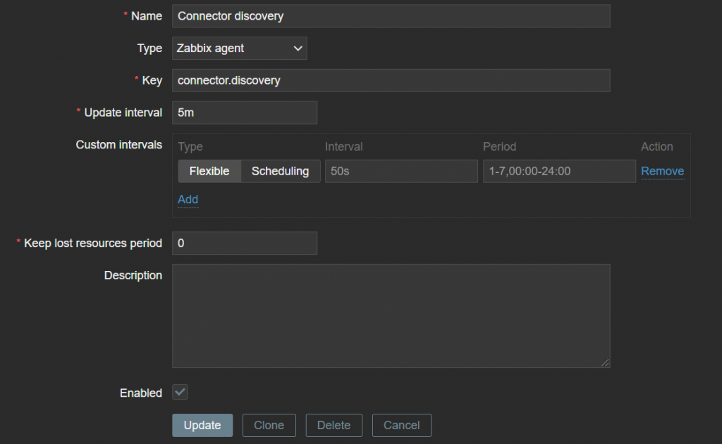
Next, we create a discovery rule. Keep lost resources period is an arbitrary value here – once again, depending on your policies regarding LLD entities.
In this case, we will discard the lost resource immediately – Keep Lost resources (0). This can be a bit more database friendly, in case when Kafka creates hundreds of connectors. The update interval is the same as the cronjob interval.
Configuration > Templates > your created template > discovery > create discovery rule
The key is used by the User Parameter further in the blog
Item prototype.
We will create two item prototypes, one for the connector and one for the task of the connector with the corresponding ID of the task. The ID is important because we want to restart the correct task later.
Name: State of {#CONNECTOR} connector
Key: state[{#CONNECTOR}]
Configuration > Templates > your created template > item prototypes > create item prototype
Trigger prototypes
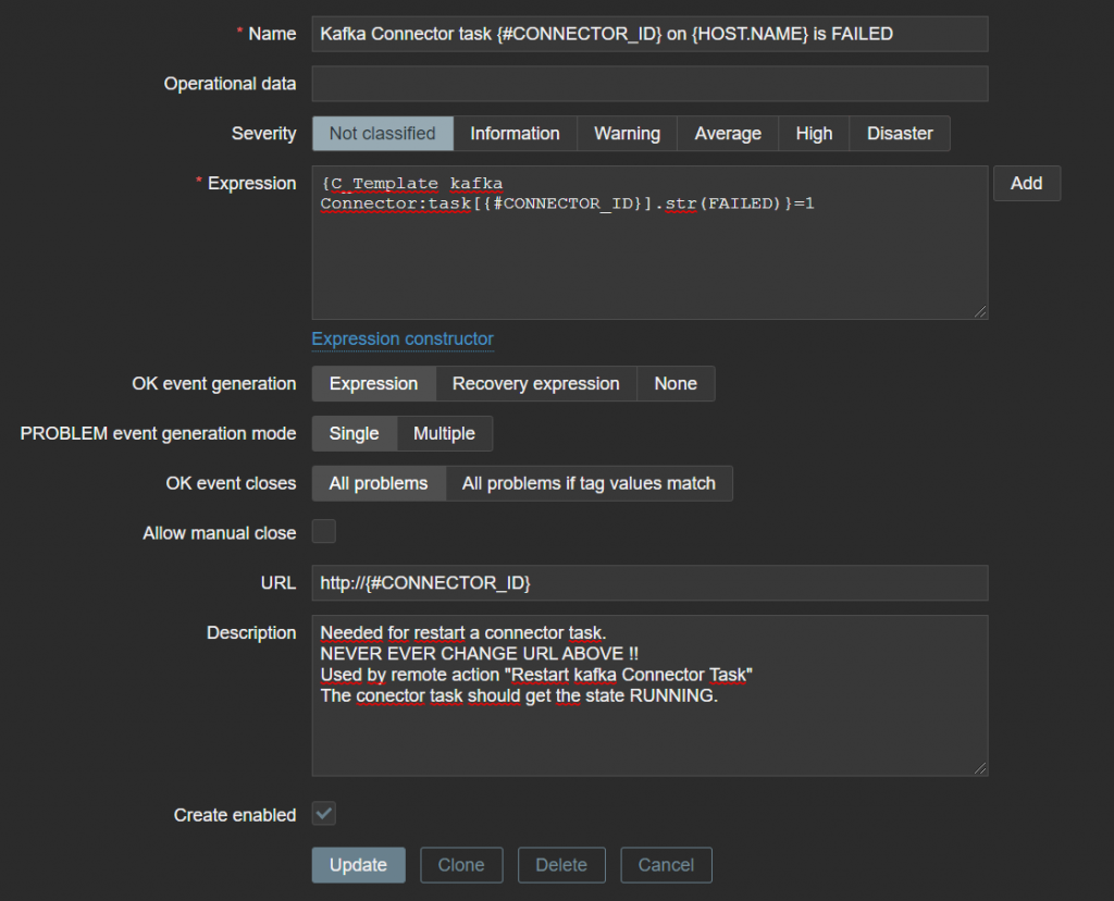
Four trigger prototypes have been created. They are sets of two. The sets have different severities. The highest severity only fires after six hours and is intended for the operation center. Most times, Zabbix will restart the failed task within 5 or 10 minutes. It is then not necessary to burden the operation center with this. I will explain the most important trigger. This trigger will soon be used in an action to start the remote command. The URL macro {TRIGGER.URL} is used, which determines the ID of the task that should be restarted. There are probably other solutions, but this one works well and is stable.
Configuration > Templates > your created template > item prototypes > create trigger prototype
The other trigger examples are provided below.
Name: Kafka Connector task {#CONNECTOR_ID} on {HOST.NAME} is not RUNNING
Expression: {C_Template kafka Connector:task[{#CONNECTOR_ID}].str(RUNNING,6h)}=0 and {C_Template kafka Connector:task[{#CONNECTOR_ID}].str(FAILED)}=1
Severity Warning
Name: Kafka Connector {#CONNECTOR} on {HOST.NAME} is FAILED
Expression: {C_Template kafka Connector:state[{#CONNECTOR}].str(FAILED)}=1
Severity: Not classified
Name: Kafka Connector {#CONNECTOR} on {HOST.NAME} is not RUNNING
Expression: {C_Template Kafka Connector:state[{#CONNECTOR}].str(RUNNING,6h)}=0 and {C_Template Kafka Connector:state[{#CONNECTOR}].str(FAILED)}=1
Severity: warning
Userparameter
Three User Parameters are required—one for the low-level discovery and two for the items.
check_task_connector.sh Does a check on the connector task. A disadvantage of this construction is that the connector can have a maximum of 10 tasks. At ID -10 or higher, the check fails. But that’s unusual in Kafka to deploy a connector with so many tasks.
When all scripts are in the right place, we make a small adjustment to the Zabbix agent config. The LogRemoteCommands option is not necessary, but it is useful for debugging. Restart the Zabbix agent afterward. Add the Kafka template to a host, and we can proceed.
EnableRemoteCommands=1
LogRemoteCommands=1
Action auto-healing
Let’s define some actions that can heal our connector tasks by automatically restarting a Kafka task with an action. Create a new action – you can choose any conditions that can be applied to your trigger.
Create an operation. This can be a bit tricky. In my case, I restart the tasks every five minutes for the first half-hour. If unsuccessful, the Kafka admins will receive an email. After that, the tasks are restarted every hour for three days. In practice, this has never happened, but such a situation can occur over the weekend, for example. After three days, the operation stops and sends a final email. Usually, the task starts the first time – if not, then the second attempt is sufficient in 99% of the cases.
Restart script.
You will probably have to adapt the script to your own environment. We have built-in some extra logging. This is certainly useful during the initial setup.
#!/bin/sh
LOG=/var/log/zabbix/restarted-connector.log
value=$(echo $1 | awk -F "/" '{print $(NF)}')
echo $value
CONNECTOR=$(echo ${value::-2})
IDS=$(echo ${value:(-1)})
curl -v -X POST http://localhost:8083/connectors/"{$CONNECTOR}"/tasks/"{$IDS}"/restart 2>&1 | tee -a $LOG
echo "Connector $CONNECTOR ID $IDS has been restarted at $(date)" >> $LOG
The {TRIGGER.URL} macro is used here, not intended to be used this way out of the box by Zabbix, but it gets the job done for this use case. The awk ensures that the http: // is fetched.
If you have any other suggestions on how to improve the scripts or the templates – you are very much welcome to leave a comment with your idea!
Credits.
I am inspired by Robin Moffatt at Confluent and not in the last place my colleague Werner Dijkerman at fullstaq
Maintaining a server fleet the size of Cloudflare’s is an operational challenge, to say the least. Anything we can do to lower complexity and improve efficiency has effects for our SRE (Site Reliability Engineer) and Data Center teams that can be felt throughout a server’s 4+ year lifespan.
At the Cloudflare Core, we process logs to analyze attacks and compute analytics. In 2020, our Core servers were in need of a refresh, so we decided to redesign the hardware to be more in line with our Gen X edge servers. We designed two major server variants for the core. The first is Core Compute 2020, an AMD-based server for analytics and general-purpose compute paired with solid-state storage drives. The second is Core Storage 2020, an Intel-based server with twelve spinning disks to run database workloads.
Core Compute 2020
Earlier this year, we blogged about our 10th generation edge servers or Gen X and the improvements they delivered to our edge in both performance and security. The new Core Compute 2020 server leverages many of our learnings from the edge server. The Core Compute servers run a variety of workloads including Kubernetes, Kafka, and various smaller services.
Configuration Changes (Kubernetes)
Previous Generation Compute
Core Compute 2020
CPU
2 x Intel Xeon Gold 6262
1 x AMD EPYC 7642
Total Core / Thread Count
48C / 96T
48C / 96T
Base / Turbo Frequency
1.9 / 3.6 GHz
2.3 / 3.3 GHz
Memory
8 x 32GB DDR4-2666
8 x 32GB DDR4-2933
Storage
6 x 480GB SATA SSD
2 x 3.84TB NVMe SSD
Network
Mellanox CX4 Lx 2 x 25GbE
Mellanox CX4 Lx 2 x 25GbE
Configuration Changes (Kafka)
Previous Generation (Kafka)
Core Compute 2020
CPU
2 x Intel Xeon Silver 4116
1 x AMD EPYC 7642
Total Core / Thread Count
24C / 48T
48C / 96T
Base / Turbo Frequency
2.1 / 3.0 GHz
2.3 / 3.3 GHz
Memory
6 x 32GB DDR4-2400
8 x 32GB DDR4-2933
Storage
12 x 1.92TB SATA SSD
10 x 3.84TB NVMe SSD
Network
Mellanox CX4 Lx 2 x 25GbE
Mellanox CX4 Lx 2 x 25GbE
Both previous generation servers were Intel-based platforms, with the Kubernetes server based on Xeon 6262 processors, and the Kafka server based on Xeon 4116 processors. One goal with these refreshed versions was to converge the configurations in order to simplify spare parts and firmware management across the fleet.
As the above tables show, the configurations have been converged with the only difference being the number of NVMe drives installed depending on the workload running on the host. In both cases we moved from a dual-socket configuration to a single-socket configuration, and the number of cores and threads per server either increased or stayed the same. In all cases, the base frequency of those cores was significantly improved. We also moved from SATA SSDs to NVMe SSDs.
Core Compute 2020 Synthetic Benchmarking
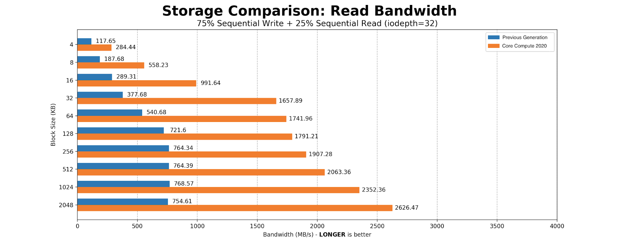
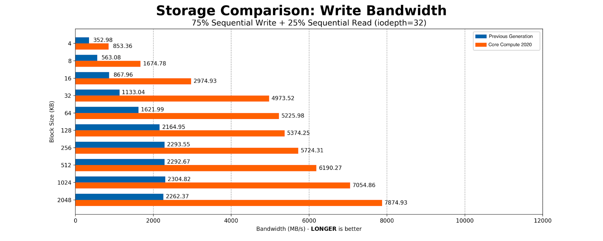
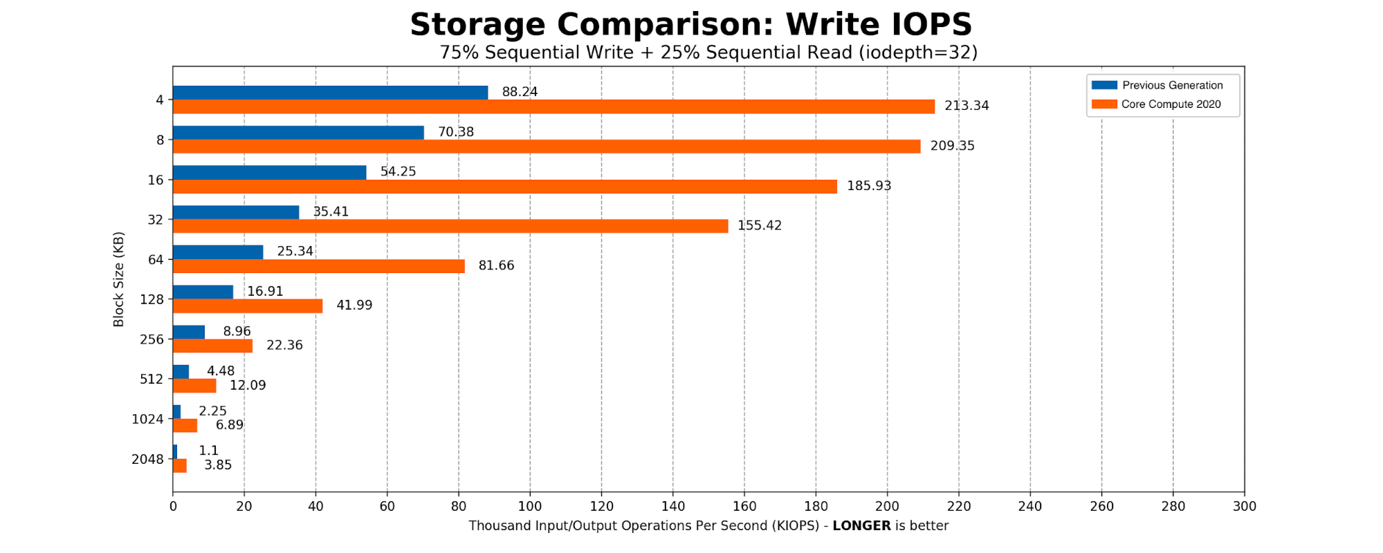
The heaviest user of the SSDs was determined to be Kafka. The majority of the time Kafka is sequentially writing 2MB blocks to the disk. We created a simple FIO script with 75% sequential write and 25% sequential read, scaling the block size from a standard page table entry size of 4096KB to Kafka’s write size of 2MB. The results aligned with what we expected from an NVMe-based drive.
Core Compute 2020 Production Benchmarking
Cloudflare runs many of our Core Compute services in Kubernetes containers, some of which are multi-core. By transitioning to a single socket, problems associated with dual sockets were eliminated, and we are guaranteed to have all cores allocated for any given container on the same socket.
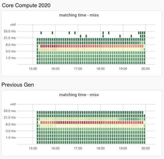
Another heavy workload that is constantly running on Compute hosts is the Cloudflare CSAM Scanning Tool. Our Systems Engineering team isolated a Compute 2020 compute host and the previous generation compute host, had them run just this workload, and measured the time to compare the fuzzy hashes for images to the NCMEC hash lists and verify that they are a “miss”.
Because the CSAM Scanning Tool is very compute intensive we specifically isolated it to take a look at its performance with the new hardware. We’ve spent a great deal of effort on software optimization and improved algorithms for this tool but investing in faster, better hardware is also important.
In these heatmaps, the X axis represents time, and the Y axis represents “buckets” of time taken to verify that it is not a match to one of the NCMEC hash lists. For a given time slice in the heatmap, the red point is the bucket with the most times measured, the yellow point the second most, and the green points the least. The red points on the Compute 2020 graph are all in the 5 to 8 millisecond bucket, while the red points on the previous Gen heatmap are all in the 8 to 13 millisecond bucket, which shows that on average, the Compute 2020 host is verifying hashes significantly faster.
Core Storage 2020
Another major workload we identified was ClickHouse, which performs analytics over large datasets. The last time we upgraded our servers running ClickHouse was back in 2018.
Configuration Changes
Previous Generation
Core Storage 2020
CPU
2 x Intel Xeon E5-2630 v4
1 x Intel Xeon Gold 6210U
Total Core / Thread Count
20C / 40T
20C / 40T
Base / Turbo Frequency
2.2 / 3.1 GHz
2.5 / 3.9 GHz
Memory
8 x 32GB DDR4-2400
8 x 32GB DDR4-2933
Storage
12 x 10TB 7200 RPM 3.5” SATA
12 x 10TB 7200 RPM 3.5” SATA
Network
Mellanox CX4 Lx 2 x 25GbE
Mellanox CX4 Lx 2 x 25GbE
CPU Changes
For ClickHouse, we use a 1U chassis with 12 x 10TB 3.5” hard drives. At the time we were designing Core Storage 2020 our server vendor did not yet have an AMD version of this chassis, so we remained on Intel. However, we moved Core Storage 2020 to a single 20 core / 40 thread Xeon processor, rather than the previous generation’s dual-socket 10 core / 20 thread processors. By moving to the single-socket Xeon 6210U processor, we were able to keep the same core count, but gained 17% higher base frequency and 26% higher max turbo frequency. Meanwhile, the total CPU thermal design profile (TDP), which is an approximation of the maximum power the CPU can draw, went down from 165W to 150W.
On a dual-socket server, remote memory accesses, which are memory accesses by a process on socket 0 to memory attached to socket 1, incur a latency penalty, as seen in this table:
Previous Generation
Core Storage 2020
Memory latency, socket 0 to socket 0
81.3 ns
86.9 ns
Memory latency, socket 0 to socket 1
142.6 ns
N/A
An additional advantage of having a CPU with all 20 cores on the same socket is the elimination of these remote memory accesses, which take 76% longer than local memory accesses.
Memory Changes
The memory in the Core Storage 2020 host is rated for operation at 2933 MHz; however, in the 8 x 32GB configuration we need on these hosts, the Intel Xeon 6210U processor clocks them at 2666 MH. Compared to the previous generation, this gives us a 13% boost in memory speed. While we would get a slightly higher clock speed with a balanced, 6 DIMMs configuration, we determined that we are willing to sacrifice the slightly higher clock speed in order to have the additional RAM capacity provided by the 8 x 32GB configuration.
Storage Changes
Data capacity stayed the same, with 12 x 10TB SATA drives in RAID 0 configuration for best throughput. Unlike the previous generation, the drives in the Core Storage 2020 host are helium filled. Helium produces less drag than air, resulting in potentially lower latency.
Core Storage 2020 Synthetic benchmarking
We performed synthetic four corners benchmarking: IOPS measurements of random reads and writes using 4k block size, and bandwidth measurements of sequential reads and writes using 128k block size. We used the fio tool to see what improvements we would get in a lab environment. The results show a 10% latency improvement and 11% IOPS improvement in random read performance. Random write testing shows 38% lower latency and 60% higher IOPS. Write throughput is improved by 23%, and read throughput is improved by a whopping 90%.
Previous Generation
Core Storage 2020
% Improvement
4k Random Reads (IOPS)
3,384
3,758
11.0%
4k Random Read Mean Latency (ms, lower is better)
75.4
67.8
10.1% lower
4k Random Writes (IOPS)
4,009
6,397
59.6%
4k Random Write Mean Latency (ms, lower is better)
63.5
39.7
37.5% lower
128k Sequential Reads (MB/s)
1,155
2,195
90.0%
128k Sequential Writes (MB/s)
1,265
1,558
23.2%
CPU frequencies
The higher base and turbo frequencies of the Core Storage 2020 host’s Xeon 6210U processor allowed that processor to achieve higher average frequencies while running our production ClickHouse workload. A recent snapshot of two production hosts showed the Core Storage 2020 host being able to sustain an average of 31% higher CPU frequency while running ClickHouse.
Previous generation (average core frequency)
Core Storage 2020 (average core frequency)
% improvement
Mean Core Frequency
2441 MHz
3199 MHz
31%
Core Storage 2020 Production benchmarking
Our ClickHouse database hosts are continually performing merge operations to optimize the database data structures. Each individual merge operation takes just a few seconds on average, but since they’re constantly running, they can consume significant resources on the host. We sampled the average merge time every five minutes over seven days, and then sampled the data to find the average, minimum, and maximum merge times reported by a Compute 2020 host and by a previous generation host. Results are summarized below.
ClickHouse merge operation performance improvement (time in seconds, lower is better)
Time
Previous generation
Core Storage 2020
% improvement
Mean time to merge
1.83
1.15
37% lower
Maximum merge time
3.51
2.35
33% lower
Minimum merge time
0.68
0.32
53% lower
Our lab-measured CPU frequency and storage performance improvements on Core Storage 2020 have translated into significantly reduced times to perform this database operation.
Conclusion
With our Core 2020 servers, we were able to realize significant performance improvements, both in synthetic benchmarking outside production and in the production workloads we tested. This will allow Cloudflare to run the same workloads on fewer servers, saving CapEx costs and data center rack space. The similarity of the configuration of the Kubernetes and Kafka hosts should help with fleet management and spare parts management. For our next redesign, we will try to further converge the designs on which we run the major Core workloads to further improve efficiency.
Special thanks to Will Buckner and Chris Snook for their help in the development of these servers, and to Tim Bart for validating CSAM Scanning Tool’s performance on Compute.
The collective thoughts of the interwebz
Manage Consent
To provide the best experiences, we use technologies like cookies to store and/or access device information. Consenting to these technologies will allow us to process data such as browsing behavior or unique IDs on this site. Not consenting or withdrawing consent, may adversely affect certain features and functions.
Functional
Always active
The technical storage or access is strictly necessary for the legitimate purpose of enabling the use of a specific service explicitly requested by the subscriber or user, or for the sole purpose of carrying out the transmission of a communication over an electronic communications network.
Preferences
The technical storage or access is necessary for the legitimate purpose of storing preferences that are not requested by the subscriber or user.
Statistics
The technical storage or access that is used exclusively for statistical purposes.The technical storage or access that is used exclusively for anonymous statistical purposes. Without a subpoena, voluntary compliance on the part of your Internet Service Provider, or additional records from a third party, information stored or retrieved for this purpose alone cannot usually be used to identify you.
Marketing
The technical storage or access is required to create user profiles to send advertising, or to track the user on a website or across several websites for similar marketing purposes.