Tag Archives: stream-processing

Enabling near real-time data analytics on the data lake

2024-02-23 Grab Tech

Post Syndicated from Grab Tech original https://engineering.grab.com/enabling-near-realtime-data-analytics

Introduction

In the domain of data processing, data analysts run their ad hoc queries on the data lake. The lake serves as an interface between our analytics and production environment, preventing downstream queries from impacting upstream data ingestion pipelines. To ensure efficient data processing in the data lake, choosing appropriate storage formats is crucial.

The vanilla data lake solution is built on top of cloud object storage with Hive metastore, where data files are written in Parquet format. Although this setup is optimised for scalable analytics query patterns, it struggles to handle frequent updates to the data due to two reasons:

The Hive table format requires us to rewrite the Parquet files with the latest data. For instance, to update one record in a Hive unpartitioned table, we would need to read all the data, update the record, and write back the entire data set.
Writing Parquet files is expensive due to the overhead of organising the data to a compressed columnar format, which is more complex than a row format.

The issue is further exacerbated by the scheduled downstream transformations. These necessary steps, which clean and process the data for use, increase the latency because the total delay now includes the combined scheduled intervals of these processing jobs.

Fortunately, the introduction of the Hudi format, which supports fast writes by allowing Avro and Parquet files to co-exist on a Merge On Read (MOR) table, opens up the possibility of having a data lake with minimal data latency. The concept of a commit timeline further allows data to be served with Atomicity, Consistency, Isolation, and Durability (ACID) guarantees.

We employ different sets of configurations for the different characteristics of our input sources:

High or low throughput. A high-throughput source refers to one that has a high level of activity. One example of this can be our stream of booking events generated from each customer transaction. On the other hand, a low-throughput source would be one that has a relative low level of activity. An example of this can be transaction events generated from reconciliation happening on a nightly basis.
Kafka (unbounded) or Relational Database Sources (bounded). Our sinks have sources that can be broadly categorised into unbounded and bounded sources. Unbounded sources are usually related to transaction events materialised as Kafka topics, representing user-generated events as they interact with the Grab superapp. Bounded sources usually refer to Relational Database (RDS) sources, whose size is bound to storage provisioned.

The following sections will delve into the differences between each source and our corresponding configurations optimised for them.

High throughput source

For our data sources with high throughput, we have chosen to write the files in MOR format since the writing of files in Avro format allows for fast writes to meet our latency requirements.

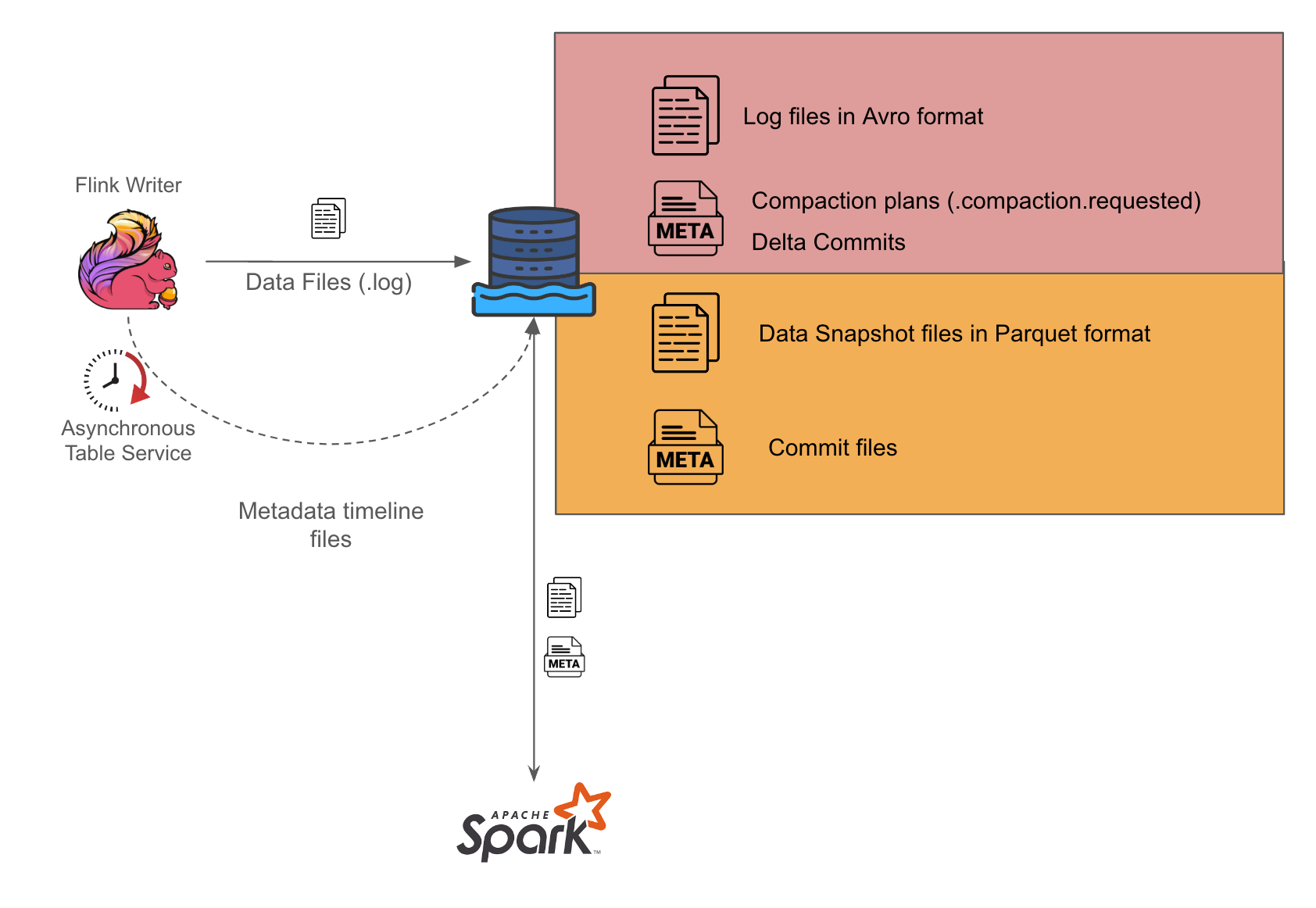
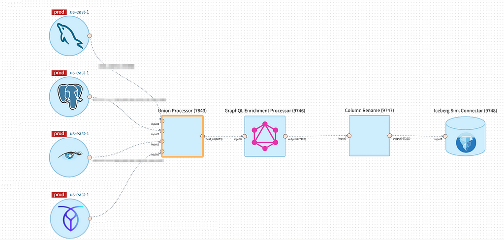
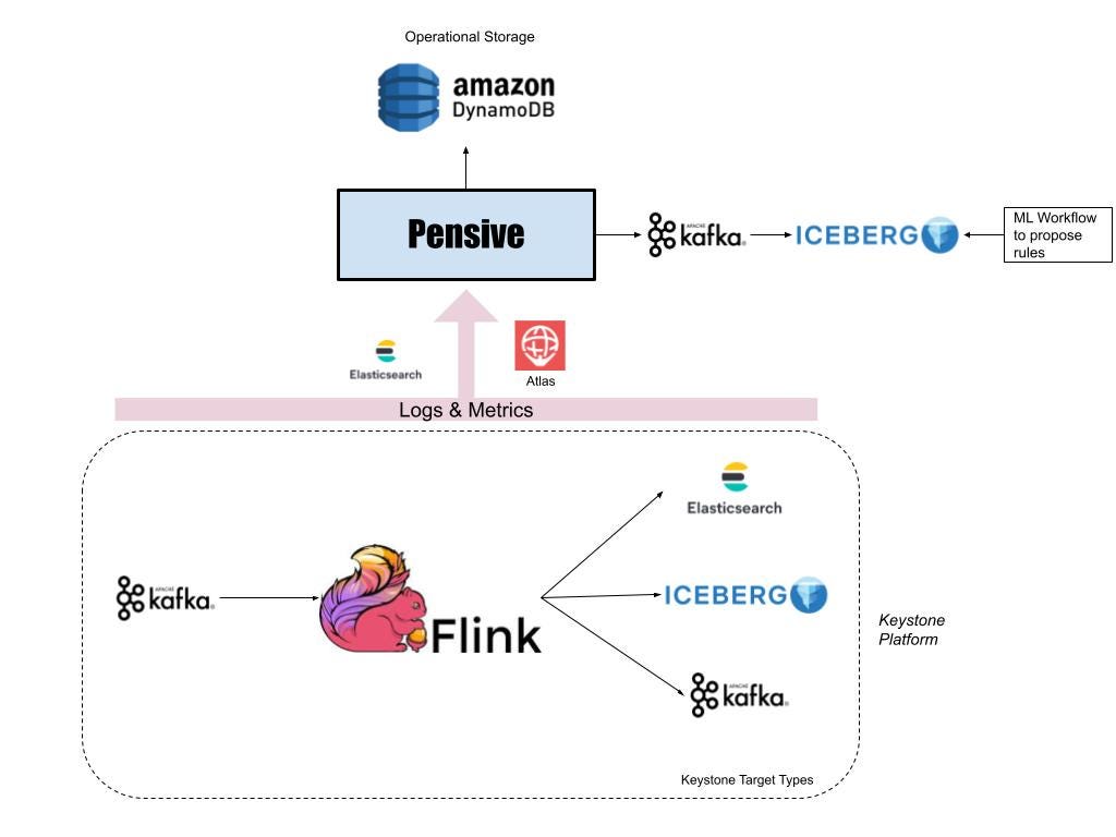
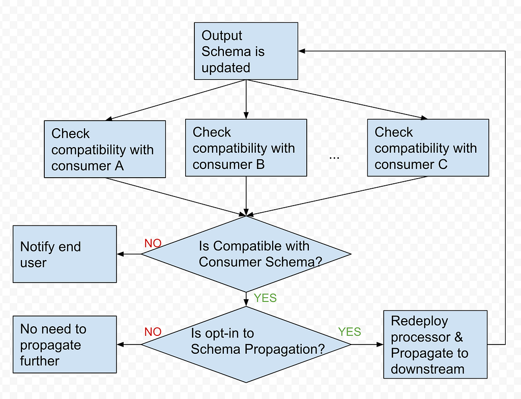
As seen in Figure 1, we use Flink to perform the stream processing and write out log files in Avro format in our setup. We then set up a separate Spark writer which periodically converts the Avro files into Parquet format in the Hudi compaction process.

We have further simplified the coordination between the Flink and Spark writers by enabling asynchronous services on the Flink writer so it can generate the compaction plans for Spark writers to act on. During the Spark job runs, it checks for available compaction plans and acts on them, placing the burden of orchestrating the writes solely on the Flink writer. This approach could help minimise potential concurrency problems that might otherwise arise, as there would be a single actor
orchestrating the associated Hudi table services.

Low throughput source

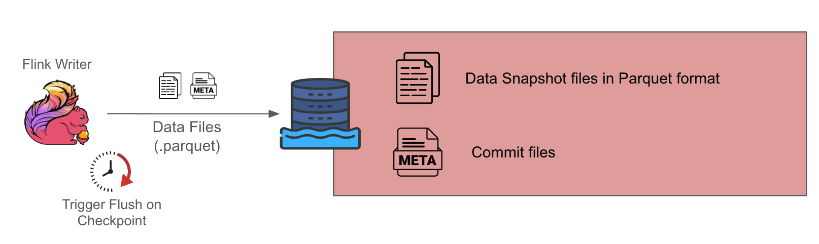
For low throughput sources, we gravitate towards the choice of Copy On Write (COW) tables given the simplicity of its design, since it only involves one component, which is the Flink writer. The downside is that it has higher data latency because this setup only generates Parquet format data snapshots at each checkpoint interval, which is typically about 10-15 minutes.

Connecting to our Kafka (unbounded) data source

Grab uses Protobuf as our central data format in Kafka, ensuring schema evolution compatibility. However, the derivation of the schema of these topics still requires some transformation to make it compatible with Hudi’s accepted schema. Some of these transformations include ensuring that Avro record fields do not contain just a single array field, and handling logical decimal schemas to transform them to fixed byte schema for Spark compatibility.

Given the unbounded nature of the source, we decided to partition it by Kafka event time up to the hour level. This ensured that our Hudi operations would be faster. Parquet file writes would be faster since they would only affect files within the same partition, and each Parquet file within the same event time partition would have a bounded size given the monotonically increasing nature of Kafka event time.

By partitioning tables by Kafka event time, we can further optimise compaction planning operations, since the amount of file lookups required is now reduced with the use of BoundedPartitionAwareCompactionStrategy. Only log files in recent partitions would be selected for compaction and the job manager need not list every partition to figure out which log files to select for compaction during the planning phase anymore.

Connecting to our RDS (bounded) data source

For our RDS, we decided to use the Flink Change Data Capture (CDC) connectors by Veverica to obtain the binlog streams. The RDS would then treat the Flink writer as a replication server and start streaming its binlog data to it for each MySQL change. The Flink CDC connector presents the data as a Kafka Connect (KC) Source record, since it uses the Debezium connector under the hood. It is then a straightforward task to deserialise these records and transform them into Hudi records, since
the Avro schema and associated data changes are already captured within the KC source record.

The obtained binlog timestamp is also emitted as a metric during consumption for us to monitor the observed data latency at the point of ingestion.

Optimising for these sources involves two phases:

First, assigning more resources for the cold start incremental snapshot process where Flink takes a snapshot of the current data state in the RDS and loads the Hudi table with that snapshot. This phase is usually resource-heavy as there are a lot of file writes and data ingested during this process.
Once the snapshotting is completed, Flink would then start to process the binlog stream and the observed throughput would drop to a level similar to the DB write throughput. The resources required by the Flink writer at this stage would be much lower than in the snapshot phase.

Indexing for Hudi tables

Indexing is important for upserting Hudi tables when the writing engine performs updates, allowing it to efficiently locate the file groups of the data to be updated.

As of version 0.14, the Flink engine only supports Bucket Index or Flink State Index. Bucket Index performs indexing of the file record by hashing the record key and matching it to a specific bucket of files indicated by the naming convention of the written data files. Flink State Index on the other hand stores the index map of record keys to files in memory.

Given that our tables include unbounded Kafka sources, there is a possibility for our state indexes to grow indefinitely. Furthermore, the requirement of state preservation for Flink State Index across version deployments and configuration updates adds complexity to the overall solution.

Thus, we opted for the simple Bucket Index for its simplicity and the fact that our Hudi table size per partition does not change drastically across the week. However, this comes with a limitation whereby the number of buckets cannot be updated easily and imposes a parallelism limit at which our Flink pipelines can scale. Thus, as traffic grows organically, we would find ourselves in a situation whereby our configuration grows obsolete and cannot handle the increased load.

To resolve this going forward, using consistent hashing for the Bucket Index would be something to explore to optimise our Parquet file sizes and allow the number of buckets to grow seamlessly as traffic grows.

Impact

Fresh business metrics

Post creation of our Hudi Data Ingestion solution, we have enabled various users such as our data analysts to perform ad hoc queries much more easily on data that has lower latency. Furthermore, Hudi tables can be seamlessly joined with Hive tables in Trino for additional context. This enabled the construction of operational dashboards reflecting fresh business metrics to our various operators, empowering them with the necessary information to quickly respond to any abnormalities (such as high-demand events like F1 or seasonal holidays).

Quicker fraud detection

Another significant user of our solution is our fraud detection analysts. This enabled them to rapidly access fresh transaction events and analyse them for fraudulent patterns, particularly during the emergence of a new attack pattern that hadn’t been detected by their rules engine. Our solution also allowed them to perform multiple ad hoc queries that involve lookbacks of various days’ worth of data without impacting our production RDS and Kafka clusters by using the data lake as the data interface, reducing the data latency to the minute level and, in turn, empowering them to respond more quickly to attacks.

What’s next?

As the landscape of data storage solutions evolves rapidly, we are eager to test and integrate new features like Record Level Indexing and the creation of Pre Join tables. This evolution extends beyond the Hudi community to other table formats such as IceBerg and DeltaLake. We remain ready to adapt ourselves to these changes and incorporate the advantages of each format into our data lake within Grab.

References

Hudi: https://hudi.apache.org/docs/next/overview/
Ververica Flink CDC: https://github.com/ververica/flink-cdc-connectors
Debezium: https://debezium.io/documentation/reference/stable/connectors/mysql.html

Join us

Grab is the leading superapp platform in Southeast Asia, providing everyday services that matter to consumers. More than just a ride-hailing and food delivery app, Grab offers a wide range of on-demand services in the region, including mobility, food, package and grocery delivery services, mobile payments, and financial services across 428 cities in eight countries.

Powered by technology and driven by heart, our mission is to drive Southeast Asia forward by creating economic empowerment for everyone. If this mission speaks to you, join our team today!

Streaming SQL in Data Mesh

2023-11-03 Netflix Technology Blog

Post Syndicated from Netflix Technology Blog original https://netflixtechblog.com/streaming-sql-in-data-mesh-0d83f5a00d08

Democratizing Stream Processing @ Netflix

By Guil Pires, Mark Cho, Mingliang Liu, Sujay Jain

Data powers much of what we do at Netflix. On the Data Platform team, we build the infrastructure used across the company to process data at scale.

In our last blog post, we introduced “Data Mesh” — A Data Movement and Processing Platform. When a user wants to leverage Data Mesh to move and transform data, they start by creating a new Data Mesh pipeline. The pipeline is composed of individual “Processors” that are connected by Kafka topics. The Processors themselves are implemented as Flink jobs that use the DataStream API.

Since then, we have seen many use cases (including Netflix Graph Search) adopt Data Mesh for stream processing. We were able to onboard many of these use cases by offering some commonly used Processors out of the box, such as Projection, Filtering, Unioning, and Field Renaming.

An example of a Data Mesh pipeline which moves and transforms data using Union, GraphQL Enrichment, and Column Rename Processor before writing to an Iceberg table.

By keeping the logic of individual Processors simple, it allowed them to be reusable so we could centrally manage and operate them at scale. It also allowed them to be composable, so users could combine the different Processors to express the logic they needed.

However, this design decision led to a different set of challenges.

Some teams found the provided building blocks were not expressive enough. For use cases which were not solvable using existing Processors, users had to express their business logic by building a custom Processor. To do this, they had to use the low-level DataStream API from Flink and the Data Mesh SDK, which came with a steep learning curve. After it was built, they also had to operate the custom Processors themselves.

Furthermore, many pipelines needed to be composed of multiple Processors. Since each Processor was implemented as a Flink Job connected by Kafka topics, it meant there was a relatively high runtime overhead cost for many pipelines.

We explored various options to solve these challenges, and eventually landed on building the Data Mesh SQL Processor that would provide additional flexibility for expressing users’ business logic.

The existing Data Mesh Processors have a lot of overlap with SQL. For example, filtering and projection can be expressed in SQL through SELECT and WHERE clauses. Additionally, instead of implementing business logic by composing multiple individual Processors together, users could express their logic in a single SQL query, avoiding the additional resource and latency overhead that came from multiple Flink jobs and Kafka topics. Furthermore, SQL can support User Defined Functions (UDFs) and custom connectors for lookup joins, which can be used to extend expressiveness.

Data Mesh SQL Processor

Since Data Mesh Processors are built on top of Flink, it made sense to consider using Flink SQL instead of continuing to build additional Processors for every transform operation we needed to support.

The Data Mesh SQL Processor is a platform-managed, parameterized Flink Job that takes schematized sources and a Flink SQL query that will be executed against those sources. By leveraging Flink SQL within a Data Mesh Processor, we were able to support the streaming SQL functionality without changing the architecture of Data Mesh.

Underneath the hood, the Data Mesh SQL Processor is implemented using Flink’s Table API, which provides a powerful abstraction to convert between DataStreams and Dynamic Tables. Based on the sources that the processor is connected to, the SQL Processor will automatically convert the upstream sources as tables within Flink’s SQL engine. User’s query is then registered with the SQL engine and translated into a Flink job graph consisting of physical operators that can be executed on a Flink cluster. Unlike the low-level DataStream API, users do not have to manually build a job graph using low-level operators, as this is all managed by Flink’s SQL engine.

SQL Experience on Data Mesh

The SQL Processor enables users to fully leverage the capabilities of the Data Mesh platform. This includes features such as autoscaling, the ability to manage pipelines declaratively via Infrastructure as Code, and a rich connector ecosystem.

In order to ensure a seamless user experience, we’ve enhanced the Data Mesh platform with SQL-centric features. These enhancements include an Interactive Query Mode, real-time query validation, and automated schema inference.

To understand how these features help the users be more productive, let’s take a look at a typical user workflow when using the Data Mesh SQL Processor.

Users start their journey by live sampling their upstream data sources using the Interactive Query Mode.
As the user iterate on their SQL query, the query validation service provides real-time feedback about the query.
With a valid query, users can leverage the Interactive Query Mode again to execute the query and get the live results streamed back to the UI within seconds.
For more efficient schema management and evolution, the platform will automatically infer the output schema based on the fields selected by the SQL query.
Once the user is done editing their query, it is saved to the Data Mesh Pipeline, which will then be deployed as a long running, streaming SQL job.

*Overview of the SQL Processor workflow.*

Users typically iterate on their SQL query multiple times before deploying it. Validating and analyzing queries at runtime after deployment will not only slow down their iteration, but also make it difficult to automate schema evolution in Data Mesh.

To address this challenge, we have implemented a query validation service that can verify a Flink SQL query and provide a meaningful error message for violations in real time. This enables users to have prompt validation feedback while they are editing the query. We leverage Apache Flink’s internal Planner classes to parse and transform SQL queries without creating a fully-fledged streaming table environment. This makes the query service lightweight, scalable, and execution agnostic.

To effectively operate thousands of use cases at the platform layer, we built opinionated guardrails to limit some functionalities of Flink SQL. We plan on gradually expanding the supported capabilities over time. We implemented the guardrails by recursively inspecting the Calcite tree constructed from user’s query. If the tree contains nodes that we currently don’t support, the query will be rejected from being deployed. Additionally, we translate Flink’s internal exceptions containing cryptic error messages into more meaningful error messages for our users. We plan on continuing our investments into improving the guardrails, as having proper guardrails help to improve the user experience. Some ideas for the future include rules to reject expensive and suboptimal queries.

To help Data Mesh users iterate quickly on their business logic, we have built the Interactive Query Mode as part of the platform. Users can start live sampling their streaming data by executing a simple `SELECT * FROM <table>` query. Using the Interactive Query Mode, Data Mesh platform will execute the Flink SQL query and display the results in the UI in seconds. Since this is a Flink SQL query on streaming data, new results will continue to be delivered to the user in real-time.

Users can continue to iterate and modify their Flink SQL query and once they’re satisfied with their query output, they can save the query as part of their stream processing pipeline.

To provide this interactive experience, we maintain an always-running Flink Session Cluster that can run concurrent parameterized queries. These queries will output their data to a Mantis sink in order to stream the results back to the user’s browser.

An animated gif showing the interactive query mode in action — *Interactive Query mode in action*

Learnings from our journey

In hindsight, we wish we had invested in enabling Flink SQL on the DataMesh platform much earlier. If we had the Data Mesh SQL Processor earlier, we would’ve been able to avoid spending engineering resources to build smaller building blocks such as the Union Processor, Column Rename Processor, Projection and Filtering Processor.

Since we’ve productionized Data Mesh SQL Processor, we’ve seen excitement and quick adoption from our Data Mesh users. Thanks to the flexibility of Flink SQL, users have a new way to express their streaming transformation logic other than writing a custom processor using the low-level DataStream API.

While Flink SQL is a powerful tool, we view the Data Mesh SQL Processor as a complimentary addition to our platform. It is not meant to be a replacement for custom processors and Flink jobs using low-level DataStream API. Since SQL is a higher-level abstraction, users no longer have control over low-level Flink operators and state. This means that if state evolution is critical to the user’s business logic, then having complete control over the state can only be done through low-level abstractions like the DataStream API. Even with this limitation, we have seen that there are many new use cases that are unlocked through the Data Mesh SQL Processor.

Our early investment in guardrails has helped set clear expectations with our users and keep the operational burden manageable. It has allowed us to productionize queries and patterns that we are confident about supporting, while providing a framework to introduce new capabilities gradually.

Future of SQL on Data Mesh

While introducing the SQL Processor to the Data Mesh platform was a great step forward, we still have much more work to do in order to unlock the power of stream processing at Netflix. We’ve been working with our partner teams to prioritize and build the next set of features to extend the SQL Processor. These include stream enrichment using Slowly-Changing-Dimension (SCD) tables, temporal joins, and windowed aggregations.

Stay tuned for more updates!

Streaming SQL in Data Mesh was originally published in Netflix TechBlog on Medium, where people are continuing the conversation by highlighting and responding to this story.

Supporting large campaigns at scale

2022-04-01 Grab Tech

Post Syndicated from Grab Tech original https://engineering.grab.com/supporting-large-campaigns-at-scale

Introduction

At Grab, we run large marketing campaigns every day. A typical campaign may require executing multiple actions for millions of users all at once. The actions may include sending rewards, awarding points, and sending messages. Here is what a campaign may look like: On 1st Jan 2022, send two ride rewards to all the users in the “heavy users” segment. Then, send them a congratulatory message informing them about the reward.

Years ago, Grab’s marketing team used to stay awake at midnight to manually trigger such campaigns. They would upload a file at 12 am and then wait for a long time for the campaign execution to complete. To solve this pain point and support more capabilities down this line, we developed a “batch job” service, which is part of our in-house real-time automation engine, Trident.

The following are some services we use to support Grab’s marketing teams:

Rewards: responsible for managing rewards.
Messaging: responsible for sending messages to users. For example, push notifications.
Segmentation: responsible for storing and retrieving segments of users based on certain criteria.

For simplicity, only the services above will be referenced for this article. The “batch job” service we built uses rewards and messaging services for executing actions, and uses the segmentation service for fetching users in a segment.

System requirements

Functional requirements

Apply a sequence of actions targeting a large segment of users at a scheduled time, display progress to the campaign manager and provide a final report.
- For each user, the actions must be executed in sequence; the latter action can only be executed if the preceding action is successful.

Non-functional requirements

Quick execution and high turnover rate.
- Definition of turnover rate: the number of scheduled jobs completed per unit time.
Maximise resource utilisation and balance server load.

For the sake of brevity, we will not cover the scheduling logic, nor the generation of the report. We will focus specifically on executing actions.

Naive approach

Let’s start thinking from the most naive solution, and improve from there to reach an optimised solution.

Here is the pseudocode of a naive action executor.

def executeActionOnSegment(segment, actions):
   for user in fetchUsersInSegment(segment):
       for action in actions:
           success := doAction(user, action)
           if not success:
               break
           recordActionResult(user, action)

def doAction(user, action):
   if action.type == "awardReward":
       rewardService.awardReward(user, action.meta)
   elif action.type == "sendMessage":
       messagingService.sendMessage(user, action.meta)
   else:
       # other action types ...

One may be able to quickly tell that the naive solution does not satisfy our non-functional requirements for the following reasons:

Execution is slow:
- The programme is single-threaded.
- Actions are executed for users one by one in sequence.
- Each call to the rewards and messaging services will incur network trip time, which impacts time cost.
Resource utilisation is low: The actions will only be executed on one server. When we have a cluster of servers, the other servers will sit idle.

Here are our alternatives for fixing the above issues:

Actions for different users should be executed in parallel.
API calls to other services should be minimised.
Distribute the work of executing actions evenly among different servers.

Note: Actions for the same user have to be executed in sequence. For example, if a sequence of required actions are (1) award a reward, (2) send a message informing the user to use the reward, then we can only execute action (2) after action (1) is successfully done for logical reasons and to avoid user confusion.

Our approach

A message queue is a well-suited solution to distribute work among multiple servers. We selected Kafka, among numerous message services, due to its following characteristics:

High throughput: Kafka can accept reads and writes at a very high speed.
Robustness: Events in Kafka are distributedly stored with redundancy, without a need to worry about data loss.
Pull-based consumption: Consumers can consume events at their own speed. This helps to avoid overloading our servers.

When a scheduled campaign is triggered, we retrieve the users from the segment in batches; each batch comprises around 100 users. We write the batches into a Kafka stream, and all our servers consume from the stream to execute the actions for the batches. The following diagram illustrates the overall flow.

Data in Kafka is stored in partitions. The partition configuration is important to ensure that the batches are evenly distributed among servers:

Number of partitions: Ensure that the number of stream partitions is greater than or equal to the max number of servers we will have in our cluster. This is because one Kafka partition can only be consumed by one consumer. If we have more consumers than partitions, some consumers will not receive any data.
Partition key: For each batch, assign a hash value as the partition key to randomly allocate batches into different partitions.

Now that work is distributed among servers in batches, we can consider how to process each batch faster. If we follow the naive logic, for each user in the batch, we need to call the rewards or messaging service to execute the actions. This will create very high QPS (queries per second) to those services, and incur significant network round trip time.

To solve this issue, we decided to build batch endpoints in rewards and messaging services. Each batch endpoint takes in a list of user IDs and action metadata as input parameters, and returns the action result for each user, regardless of success or failure. With that, our batch processing logic looks like the following:

def processBatch(userBatch, actions):
   users = userBatch
   for action in actions:
       successUsers, failedUsers = doAction(users, action)
       recordFailures(failedUsers, action)
       users = successUsers

def doAction(users, action):
   resp = {}
   if action.type == "awardReward":
       resp = rewardService.batchAwardReward(users, action.meta)
   elif action.type == "sendMessage":
       resp = messagingService.batchSendMessage(users, action.meta)
   else:
   # other action types ...

   return getSuccessUsers(resp), getFailedUsers(resp)

In the implementation of batch endpoints, we also made optimisations to reduce latency. For example, when awarding rewards, we need to write the records of a reward being given to a user in multiple database tables. If we make separate DB queries for each user in the batch, it will cause high QPS to DB and incur high network time cost. Therefore, we grouped all the users in the batch into one DB query for each table update instead.

Benchmark tests show that using the batch DB query reduced API latency by up to 85%.

Further optimisations

As more campaigns started running in the system, we came across various bottlenecks. Here are the optimisations we implemented for some major examples.

Shard stream by action type

Two widely used actions are awarding rewards and sending messages to users. We came across situations where the sending of messages was blocked because a different campaign of awarding rewards had already started. If millions of users were targeted for rewards, this could result in significant waiting time before messages are sent, ultimately leading them to become irrelevant.

We found out the API latency of awarding rewards is significantly higher than sending messages. Hence, to make sure messages are not blocked by long-running awarding jobs, we created a dedicated Kafka topic for messages. By having different Kafka topics based on the action type, we were able to run different types of campaigns in parallel.

Shard stream by country

Grab operates in multiple countries. We came across situations where a campaign of awarding rewards to a small segment of users in one country was delayed by another campaign that targeted a huge segment of users in another country. The campaigns targeting a small set of users are usually more time-sensitive.

Similar to the above solution, we added different Kafka topics for each country to enable the processing of campaigns in different countries in parallel.

Remove unnecessary waiting

We observed that in the case of chained actions, messaging actions are generally the last action in the action list. For example, after awarding a reward, a congratulatory message would be sent to the user.

We realised that it was not necessary to wait for a sending message action to complete before processing the next batch of users. Moreover, the latency of the sending messages API is lower than awarding rewards. Hence, we adjusted the sending messages API to be asynchronous, so that the task of awarding rewards to the next batch of users can start while messages are being sent to the previous batch.

Conclusion

We have architected our batch jobs system in such a way so that it can be enhanced and optimised without redoing its work. For example, although we currently obtain the list of targeted users from a segmentation service, in the future, we may obtain this list from a different source, for example, all Grab Platinum tier members.

Join us

Grab is a leading superapp in Southeast Asia, providing everyday services that matter to consumers. More than just a ride-hailing and food delivery app, Grab offers a wide range of on-demand services in the region, including mobility, food, package and grocery delivery services, mobile payments, and financial services across over 400 cities in eight countries.
Powered by technology and driven by heart, our mission is to drive Southeast Asia forward by creating economic empowerment for everyone. If this mission speaks to you, join our team today!

Abacus – Issuing points for multiple sources

2022-03-01 Grab Tech

Post Syndicated from Grab Tech original https://engineering.grab.com/abacus-issuing-points-for-multiple-sources

Introduction

Earlier in 2021 we published an article on Trident, Grab’s in-house real-time if this, then that (IFTTT) engine which manages campaigns for the Grab Loyalty Programme. The Grab Loyalty Programme encourages consumers to make Grab transactions by rewarding points when transactions are made. Grab rewards two types of points namely OVOPoints and GrabRewards Points (GRP). OVOPoints are issued for transactions made in Indonesia and GRP are for the transactions that are made in all other markets. In this article, the term GRP will be used to refer to both OVOPoints and GrabRewards Points.

Rewarding GRP is one of the main components of the Grab Loyalty Programme. By rewarding GRP, our consumers are incentivised to transact within the Grab ecosystem. Consumers can then redeem their GRP for a range of exciting items on the GrabRewards catalogue or to offset the cost of their spendings.

As we continue to grow our consumer base and our product offerings, a more robust platform is needed to ensure successful points transactions. In this post, we will share the challenges in rewarding GRP and how Abacus, our Point Issuance platform helps to overcome these challenges while managing various use cases.

Challenges

Growing number of products

The number of Grab’s product offerings has grown as part of Grab’s goal in becoming a superapp. The demand for rewarding GRP increased as each product team looked for ways to retain consumer loyalty. For this, we needed a platform which could support the different requirements from each product team.

External partnerships

Grab’s external partnerships consist of both one- and two-way point exchanges. With selected partners, Grab users are able to convert their GRP for the partner’s loyalty programme points, and the other way around.

Use cases

Besides the need to cater for the growing number of products and external partnerships, Grab needed a centralised points management system which could cater to various use cases of points rewarding. Let’s take a look at the use cases.

Any product, any points

There are many products in Grab and each product should be able to reward different GRP for different scenarios. Each product rewards GRP based on the goal they are trying to achieve.

The following examples illustrate the different scenarios:

GrabCar: Reward 100 GRP for when a driver cancels a booking as a form of compensation or to reward GRP for every ride a consumer makes.

GrabFood: Reward consumers for each meal order.

GrabPay: Reward consumers three times the number of GRP for using GrabPay instead of cash as the mode of payment.

More points for loyal consumers

Another use case is to reward loyal consumers with more points. This incentivises consumers to transact within the Grab ecosystem. One example are membership tiers granted based on the number of GRP a consumer has accumulated. There are four membership tiers: Member, Silver, Gold and Platinum.

There are different points multipliers for different membership tiers. For example, a Gold member would earn 2.25 GRP for every dollar spent while a Silver member earns only 1.5 GRP for the same amount spent. A consumer can view their membership tier and GRP information from the account page on the Grab app.

*GrabRewards Points and membership tier information*

Growing number of transactions

Teams within Grab and external partners use GRP in their business. There is a need for a platform that can process millions of transactions every day with high availability rates. Errors can easily impact the issuance of points which may affect our consumers’ trust.

Our solution – Abacus

To overcome the challenges and cater for various use cases, we developed a Points Management System known as Abacus. It offers an interface for external partners with the capability to handle millions of daily transactions without significant downtime.

Points rewarding

There are seven main components of Abacus as shown in the following architectural diagram. Details of each component are explained in this section.

Transaction input source

The points rewarding process begins when a transaction is complete. Abacus listens to streams for completed transactions on the Grab platform. Each transaction that abacus receives in the stream carries the data required to calculate the GRP to be rewarded such as country ID, product ID, and payment ID etc.

Apart from computing the number of GRP to be rewarded for a transaction and then rewarding the points, Abacus also allows clients from within the Grab platform and outside of the Grab platform to make an API call to reward GRP to consumers. The client who wants to reward their consumers with GRP will call Abacus with either a specific point value (for example 100 points) or will provide the necessary details like transaction amount and the relevant multipliers for Abacus to compute the points and then reward them.

Point Calculation module

The Point Calculation module calculates the GRP using the data and multipliers that are unique to each transaction.

Point Calculation dependencies for internal services

Point Calculation dependencies are the multipliers needed to calculate the number of points. The Point Calculation module fetches the correct point multipliers for each transaction. The multipliers are configured by specific country teams when the product is launched. They may vary by country to allow country teams the flexibility to achieve their growth and retention targets. There are different types of multipliers.

Vertical multiplier: The multiplier for each vertical. A vertical is a service or product offered by Grab. Examples of verticals are GrabCar and GrabFood. The multiplier can be different for each vertical.

EPPF multiplier: The effective price per fare multiplier. EPPF is the reference conversion rate per point. For example:

EPPF = 1.0; if you are issuing X points per SGD1
EPPF = 0.1; if you are issuing X points per THB10
EPPF = 0.0001; if you are issuing X points per IDR10,000

Payment Type multiplier: The multiplier for different modes of payments.

Tier multiplier: The multiplier for each tier.

Point Calculation formula for internal clients

The Point Calculation module uses a formula to calculate GRP. The formula is the product of all the multipliers and the transaction amount.

GRP = Amount * Vertical multiplier * EPPF multiplier * Cashless multiplier * Tier multiplier

The following are examples for calculating GRP:

Example 1:

Bob is a platinum member of Grab. He orders lunch in Singapore for SGD15 using GrabPay as the payment method. Let’s assume the following:

Vertical multiplier = 2

EPPF multiplier = 1

Cashless multiplier = 2

Tier multiplier = 3

GRP = Amount * Vertical multiplier * EPPF multiplier * Cashless multiplier * Tier multiplier

= 15 * 2 * 1 * 2 * 3

= 180

From this transaction, Bob earns 180 GRP.

Example 2:

Jane is a Gold member of Grab. She orders lunch in Indonesia for Rp150000 using GrabPay as the payment method. Let’s assume the following:

Vertical multiplier = 2

EPPF multiplier = 0.00005

Cashless multiplier = 2

Tier multiplier = 2

GRP = Amount * Vertical multiplier * EPPF multiplier * Cashless multiplier * Tier multiplier

= 150000 * 2 * 0.00005 * 2 * 2

= 60

From this transaction, Jane earns 60 GRP.

*Example of multipliers for payment options and tiers*

Point Calculation dependencies for external clients

External partners supply the Point Calculation dependencies which are then configured in our backend at the time of integration. These external partners can set their own multipliers instead of using the above mentioned multipliers which are specific to Grab. This document details the APIs which are used to award points for external clients.

Simple Queue Service

Abacus uses Amazon Simple Queue Service (SQS) to ensure that the points system process is robust and fault tolerant.

Point Awarding SQS

If there are no errors during the Point Calculation process, the Point Calculation module will send a message containing the points to be awarded to the Point Awarding SQS.

Retry SQS

The Point Calculation module may not receive the required data when there is a downtime in the Point Calculation dependencies. If this occurs, an error is triggered and the Point Calculation module will send a message to Retry SQS. Messages sent to the Retry SQS will be re-processed by the Point Calculation module. This ensures that the points are properly calculated despite having outages on dependencies. Every message that we push to either the Point Awarding SQS or Retry SQS will have a field called Idempotency key which is used to ensure that we reward the points only once to a particular transaction.

Point Awarding module

The successful calculation of GRP triggers a message to the Point Awarding module via the Point SQS. The Point Awarding module tries to reward GRP to the consumer’s account. Upon successful completion, an ACK is sent back to the Point SQS signalling that the message was successfully processed and triggers deletion of the message. If Point SQS does not receive an ACK, the message is redelivered after an interval. This process ensures that the points system is robust and fault tolerant.

Ledger

GRP is rewarded to the consumer once it is updated in the Ledger. The Ledger tracks how many GRP a consumer has accumulated, what they were earned for, and the running total number of GRP.

Notification service

Once the Ledger is updated, the Notification service sends the consumer a message about the GRP they receive.

Point Kafka stream

For all successful GRP transactions, Abacus sends a message to the Point Kafka stream. Downstream services listen to this stream to identify the consumer’s behaviour and take the appropriate actions. Services of this stream can listen to events they are interested in and execute their business logic accordingly. For example, a service can use the information from the Point Kafka stream to determine a consumer’s membership tier.

Points expiry

Further addition to Abacus is the handling of points expiry. The Expiry Extension module enables activity-based points expiry. This enables GRP to not expire as long as the consumer makes one Grab transaction within the next three or six months from their last transaction.

The Expiry Extension module updates the point expiry date to the database after successfully rewarding GRP to the consumer. At the end of each month, a process loads all consumers whose points will expire in that particular month and sends it to the Point Expiry SQS. The Point Expiry Consumer will then expire all the points for the consumers and this data is updated in the Ledger. This process repeats on a monthly basis.

Points expiry date is always the last day of the third or sixth month. For example, Adam makes a transaction on 10 January. His points expiry date is 31 July which is six months from the month of his last transaction. Adam then makes a transaction on 28 February. His points expiry period is shifted by one month to 31 August.

Conclusion

The Abacus platform enables us to perform millions of GRP transactions on a daily basis. Being able to curate rewards for consumers increases the value proposition of our products and consumer retention. If you have any comments or questions about Abacus, feel free to leave a comment below.

Special thanks to Arianto Wibowo and Vaughn Friesen.

Join us

Powered by technology and driven by heart, our mission is to drive Southeast Asia forward by creating economic empowerment for everyone. If this mission speaks to you, join our team today!

Auto-Diagnosis and Remediation in Netflix Data Platform

2022-01-14 Netflix Technology Blog

Post Syndicated from Netflix Technology Blog original https://netflixtechblog.com/auto-diagnosis-and-remediation-in-netflix-data-platform-5bcc52d853d1

By Vikram Srivastava and Marcelo Mayworm

Netflix has one of the most complex data platforms in the cloud on which our data scientists and engineers run batch and streaming workloads. As our subscribers grow worldwide and Netflix enters the world of gaming, the number of batch workflows and real-time data pipelines increases rapidly. The data platform is built on top of several distributed systems, and due to the inherent nature of these systems, it is inevitable that these workloads run into failures periodically. Troubleshooting these problems is not a trivial task and requires collecting logs and metrics from several different systems and analyzing them to identify the root cause. At our scale, even a tiny percentage of disrupted workloads can generate a substantial operational support burden for the data platform team when troubleshooting involves manual steps. And we can’t discount the productivity impact it causes on data platform users.

It motivates us to be proactive in detecting and handling failed workloads in our production environment, avoiding interruptions that could slow down our teams. We have been working on an auto-diagnosis and remediation system called Pensive in the data platform to address these concerns. With the goal of troubleshooting failing and slow workloads and remediating them without human intervention wherever possible. As our platform continues to grow and different scenarios and issues can disrupt the workloads, Pensive has to be proactive in detecting broad problems at the platform level in real-time and diagnosing the impact across the workloads.

Pensive infrastructure comprises two separate systems to support batch and streaming workloads. This blog will explore these two systems and how they perform auto-diagnosis and remediation across our Big Data Platform and Real-time infrastructure.

Batch Pensive

Batch workflows in the data platform run using a Scheduler service that launches containers on the Netflix container management platform called Titus to run workflow steps. These steps launch jobs on clusters running Apache Spark and Presto via Genie. If a workflow step fails, Scheduler asks Pensive to diagnose the step’s error. Pensive collects logs for the failed jobs launched by the step from the relevant data platform components and then extracts the stack traces. Pensive relies on a regular expression based rules engine that has been curated over time. The rules encode information about whether an error is due to a platform issue or a user bug and whether the error is transient or not. If a regular expression from one of the rules matches, then Pensive returns information about that error to the Scheduler. If the error is transient, Scheduler will retry that step with exponential backoff a few more times.

The most critical part of Pensive is the set of rules used to classify an error. We need to evolve them as the platform evolves to ensure that the percentage of errors that Pensive cannot classify remains low. Initially, the rules were added on an ad-hoc basis as requests came in from platform component owners and users. We have now moved to a more systematic approach where unknown errors are fed into a Machine Learning process that performs clustering to propose new regular expressions for commonly occurring errors. We take the proposals to platform component owners to then come up with the classification of the error source and whether it is of transitory nature. In the future, we are looking to automate this process.

Detection of Platform-wide Issues

Pensive does error classification on individual workflow step failures, but by doing real-time analytics on the errors detected by Pensive using Apache Kafka and Apache Druid, we can quickly identify platform issues affecting many workflows. Once the individual diagnoses get stored in a Druid table, our monitoring and alerting system called Atlas does aggregations every minute and sends out alerts if there is a sudden increase in the number of failures due to platform errors. This has led to a dramatic reduction in the time it takes to detect issues in hardware or bugs in recently rolled out data platform software.

Streaming Pensive

Apache Flink powers real-time stream processing jobs in the Netflix data platform. And most of the Flink jobs run under a managed platform called Keystone, which abstracts out the underlying Flink job details and allows users to consume data from Apache Kafka streams and publish them to different data stores like Elasticsearch and Apache Iceberg on AWS S3.

Since the data platform manages keystone pipelines, users expect platform issues to be detected and remediated by the Keystone team without any involvement from their end. Furthermore, data in Kafka streams have a finite retention period, which adds time pressure for resolving the issues to avoid data loss.

For every Flink job running as part of a Keystone pipeline, we monitor the metric indicating how far the Flink consumer lags behind the Kafka producer. If it crosses a threshold, Atlas sends a notification to Streaming Pensive.

Like its batch counterpart, Streaming Pensive also has a rules engine to diagnose errors. However, in addition to logs, Streaming Pensive also has rules for checking various metric values for multiple components in the Keystone pipeline. The issue may occur in the source Kafka stream, the main Flink job, or the sinks to which the Flink job is writing data. Streaming Pensive diagnoses it and tries to remediate the issue automatically when it happens. Some examples where we are able to auto-remediate are:

If Streaming Pensive finds that one or more Flink Task Managers are going out of memory, it can redeploy the Flink cluster with more Task Managers.
If Streaming Pensive finds that there is an unexpected increase in the rate of incoming messages on the source Kafka cluster, it can increase the topic retention size and period so that we don’t lose any data while the consumer is lagging. If the spike goes away after some time, Streaming Pensive can revert the retention changes. Otherwise, it will page the job owner to investigate if there is a bug causing the increased rate or if the consumers need to be reconfigured to handle the higher rate.

Even though we have a high success rate, there are still occasions where automation is not possible. If manual intervention is required, Streaming Pensive will page the relevant component team to take timely action to resolve the issue.

What’s Next?

Pensive has had a significant impact on the operability of the Netflix data platform. And helped engineering teams lower the burden of operations work, freeing them to tackle more critical and challenging problems. But our job is nowhere near done. We have a long roadmap ahead of us. Some of the features and expansions we have planned are:

Batch Pensive is currently diagnosing failed jobs only, and we want to increase the scope into optimization to determine why jobs have become slow.
Auto-configure batch workflows so that they finish successfully or become faster and use fewer resources when possible. One example where it can dramatically help is Spark jobs, where memory tuning is a significant challenge.
Expand Pensive with Machine Learning classifiers.
The streaming platform recently added Data Mesh, and we need to expand Streaming Pensive to cover that.

Acknowledgments

This work could not have been completed without the help of the Big Data Compute and the Real-time Data Infrastructure teams within the Netflix data platform. They have been great partners for us as we work on improving the Pensive infrastructure.

Auto-Diagnosis and Remediation in Netflix Data Platform was originally published in Netflix TechBlog on Medium, where people are continuing the conversation by highlighting and responding to this story.

Data Movement in Netflix Studio via Data Mesh

2021-07-26 Netflix Technology Blog

Post Syndicated from Netflix Technology Blog original https://netflixtechblog.com/data-movement-in-netflix-studio-via-data-mesh-3fddcceb1059

By Andrew Nguonly, Armando Magalhães, Obi-Ike Nwoke, Shervin Afshar, Sreyashi Das, Tongliang Liu, Wei Liu, Yucheng Zeng

Background

Over the next few years, most content on Netflix will come from Netflix’s own Studio. From the moment a Netflix film or series is pitched and long before it becomes available on Netflix, it goes through many phases. This happens at an unprecedented scale and introduces many interesting challenges; one of the challenges is how to provide visibility of Studio data across multiple phases and systems to facilitate operational excellence and empower decision making. Netflix is known for its loosely coupled microservice architecture and with a global studio footprint, surfacing and connecting the data from microservices into a studio data catalog in real time has become more important than ever.

Operational Reporting is a reporting paradigm specialized in covering high-resolution, low-latency data sets, serving detailed day-to-day activities¹ and processes of a business domain. Such a paradigm aspires to assist front-line operations personnel and stakeholders in “running the business”²; performing their tasks through means such as ad hoc analysis, decision-support, and tracking (of tasks, assets, schedules, etc). The paradigm spans across methods, tools, and technologies and is usually defined in contrast to analytical reporting and predictive modeling which are more strategic (vs. tactical) in nature.

At Netflix Studio, teams build various views of business data to provide visibility for day-to-day decision making. With dependable near real-time data, Studio teams are able to track and react better to the ever-changing pace of productions and improve efficiency of global business operations using the most up-to-date information. Data connectivity across Netflix Studio and availability of Operational Reporting tools also incentivizes studio users to avoid forming data silos.

The Journey

In the past few years, Netflix Studio has gone through few iterations of data movement approaches. In the initial stage, data consumers set up ETL pipelines directly pulling data from databases. With this batch style approach, several issues have surfaced like data movement is tightly coupled with database tables, database schema is not an exact mapping of business data model, and data being stale given it is not real time etc. Later on, we moved to event driven streaming data pipelines (powered by Delta), which solved some problems compared to the batch style, but had its own pain points, such as a high learning curve of stream processing technologies, manual pipeline setup, a lack of schema evolution support, inefficiency of onboarding new entities, inconsistent security access models, etc.

With the latest Data Mesh Platform, data movement in Netflix Studio reaches a new stage. This configuration driven platform decreases the significant lead time when creating a new pipeline, while offering new support features like end-to-end schema evolution, self-serve UI and secure data access. The high level diagram below indicates the latest version of data movement for Operational Reporting.

Operational Reporting Architecture Overview

For data delivery, we leverage the Data Mesh platform to power the data movement. Netflix Studio applications expose GraphQL queries via Studio Edge, which is a unified graph that connects all data in Netflix Studio and provides consistent data retrieval. Change Data Capture(CDC) source connector reads from studio applications’ database transaction logs and emits the change events. The CDC events are passed on to the Data Mesh enrichment processor, which issues GraphQL queries to Studio Edge to enrich the data. Once the data has landed in the Iceberg tables in Netflix Data Warehouse, they could be used for ad-hoc or scheduled querying and reporting. Centralized data will be moved to third party services such as Google Sheets and Airtable for the stakeholders. We will deep dive into Data Delivery and Data Consumption in the following sections.

Data Delivery via Data Mesh

What is Data Mesh?

Data Mesh is a fully managed, streaming data pipeline product used for enabling Change Data Capture (CDC) use cases. In Data Mesh, users create sources and construct pipelines. Sources mimic the state of an externally managed source — as changes occur in the external source, corresponding CDC messages are produced to the Data Mesh source. Pipelines can be configured to transform and store data to externally managed sinks.

Data Mesh provides a drag-and-drop, self-service user interface for exploring sources and creating pipelines so that users can focus on delivering business value without having to worry about managing and scaling complex data streaming infrastructure.

CDC and data source

Change data capture or CDC, is a semantic for processing changes in a source for the purpose of replicating those changes to a sink. The table changes could be row changes (insert row, update row, delete row) or schema changes (add column, alter column, drop column). As of now, CDC sources have been implemented for data stores at Netflix (MySQL, Postgres). CDC events can also be sent to Data Mesh via a Java Client Producer Library.

Reusable Processors and Configuration Driven

In Data Mesh, a processor is a configurable data processing application that consumes, transforms, and produces CDC events. A processor has 1 or more inputs and 0 or more outputs. Processors with 0 outputs are sink connectors; which write events to externally managed sinks (e.g. Iceberg, ElasticSearch, etc).

Processors with Different Inputs/Outputs

Data Mesh allows developers to contribute processors to the platform. Processors are not necessarily centrally developed and managed. However, the Data Mesh platform team strives to provide and manage the most highly leveraged processors (e.g. source connectors and sink connectors)

Processors are reusable. The same processor image package is used multiple times for all instances of the processor. Each instance is configured to fit each use case. For example, a GraphQL enrichment processor can be provisioned to query GraphQL Services to enrich data in different pipelines; an Iceberg sink processor can be initialized multiple times to write data to different databases/tables with different schema.

End-to-End Schema Evolution

Schema is a key component of Data Mesh. When an upstream schema evolves (e.g. schema change in the MySQL table), Data Mesh detects the change, checks the compatibility and applies the change to the downstream. With schema evolution, Data Mesh ensures the Operational Reporting pipelines always produce data with the latest schema.

We will cover a few core concepts in the Data Mesh Schema domain.

Consumer schema
Consumer schema defines how data is consumed by the downstream processors. See example below.

Schema Compatibility
Data Mesh uses Consumer Schema compatibility to achieve flexible yet safe schema evolution. If a field consumed by an Operational Reporting pipeline is removed from CDC source, Data Mesh categorizes this change as incompatible, pauses the pipeline processing and notifies the pipeline owner. On the other hand, if a required field is not consumed by any consumer, dropping such fields would be compatible.

Two Types of Processors
1. Pass through all fields from upstream to downstream.

Example: Filter Processor, Sink Processors

2. Only uses a subset of fields from upstream.

Example: Project Processor, Enrichment Processor

In Data Mesh, we introduce the Opt-in to Schema Evolution boolean flag to differentiate those two types of use cases.

Opt in: All the upstream fields will be propagated to the processor. For example, when a new field is added upstream, it will be propagated automatically.
Opt out: Only a subset of fields (defined using ‘Is Consumed’ checkboxes) is propagated and used in the processor. Upstream changes to the rest of the fields won’t affect this processor.

Schema Propagation
After the Schema Compatibility is checked, Data Mesh Platform will propagate the schema change based on the end user’s intention. With the opt-in to schema Evolution flag, Operational Reporting pipelines can keep the schema up-to-date with upstream data stores. As part of schema propagation, the platform also syncs the schema from the pipeline to the Iceberg sink.

Enrichment Processor via GraphQL

In the current Data Mesh Operational Reporting pipelines, the most commonly used intermediate processor is the GraphQL Enrichment Processor. It takes in the column value from CDC events coming from Source Connector as GraphQL query input, then submits a query to Studio Edge to enrich the data. With Studio Edge’s single data model, it centralizes data modeling efforts, which is highly leveraged by Studio UI Apps, Backend services and Search platforms. Enriching the data via Studio Edge helps us achieve consistent data modeling across the whole ecosystem for Operational Reporting.

Here is the example of GraphQL processor configuration, pipeline builder only need config the following fields to provision an enrichment processor:

GraphQL Enrichment Processor Configuration Example

The image below is a sample Operational Reporting pipeline in the production environment to sink the Movie related data. Teams who want to move their data no longer need to learn and write customized Stream Processing jobs. Instead they just need to configure the pipeline topology in the UI while getting other features like schema evolution and secure data access out of the box.

Iceberg Sink

Apache Iceberg is an open source table format for huge analytics datasets. Data Mesh leverages Iceberg tables as data warehouse sinks for downstream analytics use cases. Currently Iceberg sink is appended only. Views are built on top of the raw Iceberg tables to retrieve the latest record for every primary key based on the operational timestamp, which indicates when the record is produced in the sink. Current pipeline consumers are directly consuming Views instead of raw tables.

The compaction process is needed to optimize the performance of downstream queries on the business view as well as lower costs of S3 GET OBJECT operations. A daily process ranks the records by timestamp to generate a data frame of compacted records. Old data files are overwritten with a set of new data files that contain only the compacted data.

Data Quality

Data Mesh provides metrics and dashboards at both the processor and pipeline level for operational observability. Operational Reporting pipeline owners will get alerts if something goes wrong with their pipelines. We also have two types of auditing on the data tables generated from Data Mesh pipelines to guarantee data quality: end-to-end auditing and synthetic events.

Most of the business views created on top of the Iceberg tables can tolerate a few minutes of latency. However, it is paramount that we validate the complete set of identifiers such as a list of movie ids across producers and consumers for higher overall confidence in the data transport layer of choice. For end-to-end audits, the objective is to run the audits hourly via Big data Platform Scheduler, which is a centralized and integrated tool provided by Netflix data platform for running workflows in an efficient, reliable and reproducible way. The audits check for equality (i.e. query results should be the same), the symmetric difference between two data sets should be empty across multiple runs, and the eventual consistency within the SLA. An hourly notification is sent when a set of primary keys consistently do not match between source of truth and target Data Mesh tables.

Synthetic events audits are artificially triggered change events to imitate common CUD operations of services. It is generating heartbeat signals at a constant frequency with the objective of using them as a baseline to verify the health of the pipeline regardless of traffic patterns or occasional silences.

Data Consumption

Our studio partners rely on data to make informed decisions and to collaborate during all the phases related to production. The Studio Tech Solutions team provides near real-time reports in some data tool of choice, which we call trackers to empower the decision making.

For the past few years, many of these trackers were powered by hand-curated SQL scripts and API calls being managed by CRON schedulers implemented in a Java Service called Lego. Lego was the main tool for the STS team, and at its peak, Lego managed 300+ trackers.

This strategy had its own set of challenges: being schema-less and treating every report column like a string not always worked out, the volatile reliance on direct RDS connections and rate limits from third party APIs would often make jobs fail. We had a set of “core views” which would be specifically tailored for reports, but this caused queries that just required a very small subset of fields to be slow and expensive due to the view doing a huge amount of joining and aggregation work before being able to retrieve that small subset.

Besides the issues, this worked fine when we didn’t have many trackers to maintain, but as we created more trackers to the point of having many hundreds, we started having issues around maintenance, awareness, knowledge sharing and standardization. New team members had a hard time getting onboard, figuring out which SQL powered which tracker was tough, the lack of standards made every SQL look different and having to update trackers as the data sources changed was a nightmare.

With this in mind, the Studio Tech Solutions focused efforts in building Genesis, a Semantic Data Layer that allows the team to map data points in Data Source Definitions defined as YAML files and then use those to generate the SQL needed for the trackers, based on a selection of fields, filters and formatters specified in an Input Definition file. Genesis takes care of joining, aggregating, formatting and filtering data based on what is available in the Data Source Definitions and specified by the user through the Input Definition being executed.

Genesis Data Source and Input definition example

Genesis is a stateless CLI written in Node.js that reads everything it needs from the file system based on the paths specified in the arguments. This allows us to hook Genesis into Jenkins Jobs, providing a GitOps and CI experience to maintain existing trackers, as well as create new trackers. We can simply change the data layer, trigger an empty pull request, review the changes and have all our trackers up to date with the data source changes.

As of the date of writing, Genesis powers 240+ trackers and is growing everyday, empowering thousands of partners in our studios globally to collaborate, annotate and share information using near-real-time data.

Git-based Tracker management workflow powered by Genesis and the Big Data Scheduler

The generated queries are then used in Workflow Definitions for multiple trackers. The Netflix Data Warehouse offers support for users to create data movement workflows that are managed through our Big Data Scheduler, powered by Titus.

We use the scheduler to execute our queries and move the results to a data tool, which often is a Google Sheet Tab, Airtable base or Tableau dashboard. The scheduler offers templated jobs for moving data from a Presto SQL output to these tools, making it easy to create and maintain hundreds of data movement workflows.

The diagram below summarizes the data consumption flow when building trackers:

As of July 2021, the Studio Tech Solutions team is finishing a migration from all the trackers built in Lego to use Genesis and the Data Portal. This strategy has increased the Studio Tech Solutions team performance and stability. Trackers are now easy for the team to create, review, change, monitor and discover.

Now and Future

In conclusion, our studio partners have a tracker available to them, populated with near real-time data and tailored to their needs. They can manipulate, annotate, and collaborate using a flexible tool they are familiar with.

Along the journey, we have learned that evolving data movement in complex domains could take multiple iterations and needs to be driven by the business impact. The great cross-functional partnership and collaboration among all data stakeholders is crucial to shape the ideal data product.

However, our story doesn’t end here. We still have a long journey ahead of us to fulfill the vision of such ideal data product, especially in areas such as:

Self-servicing data pipelines provisioning via configuration
Providing toolings for data discoverability, understandability, usage visibility and change management
Enabling data domain orientation and ownership/governance management
Bootstrapping trackers in our Studio ecosystem instead of third party tools. Along the same line as the point above, this would allow us to maintain high standards of data governance, lineage, and security.
Read-write reports and trackers using GraphQL mutations

These are some of the interesting areas that Netflix Studio is planning to invest in. We will have follow up blog posts on these topics in future. Please stay tuned!

Endnotes

¹ Inmon, Bill. Operational and Informational Reporting, Information Management, July 1st, 2000.
² Dehghani, Zhamak. Data Mesh: Delivering Data-driven Value at Scale, O’Reilly Media, Inc., 2021.

Acknowledgements

Data Movement via Data Mesh has been a success in Netflix Studio owing to multiple teams’ efforts. We would like to acknowledge the following colleagues: Amanda Benhamou, Andreas Andreakis, Anthony Preza, Bo Lei, Charles Zhao, Justin Cunningham, Kasturi Chatterjee, Kevin Zhu, Stephanie Barreyro, Yoomi Koh.

Data Movement in Netflix Studio via Data Mesh was originally published in Netflix TechBlog on Medium, where people are continuing the conversation by highlighting and responding to this story.

Optimally scaling Kafka consumer applications

2020-10-13 Grab Tech

Post Syndicated from Grab Tech original https://engineering.grab.com/optimally-scaling-kafka-consumer-applications

Earlier this year, we took you on a journey on how we built and deployed our event sourcing and stream processing framework at Grab. We’re happy to share that we’re able to reliably maintain our uptime and continue to service close to 400 billion events a week. We haven’t stopped there though. To ensure that we can scale our framework as the Grab business continuously grows, we have spent efforts optimizing our infrastructure.

In this article, we will dive deeper into our Kubernetes infrastructure setup for our stream processing framework. We will cover why and how we focus on optimal scalability and availability of our infrastructure.

Quick Architecture Recap

The Coban platform provides lightweight Golang plugin architecture-based data processing pipelines running in Kubernetes. These are essentially Kafka consumer pods that consume data, process it, and then materialize the results into various sinks (RDMS, other Kafka topics).

Anatomy of a Processing Pod

Each stream processing pod (the smallest unit of a pipeline’s deployment) has three top level components:

Trigger: An interface that connects directly to the source of the data and converts it into an event channel.
Runtime: This is the app’s entry point and the orchestrator of the pod. It manages the worker pools, triggers, event channels, and lifecycle events.
Pipeline plugin: This is provided by the user, and conforms to a contract that the platform team publishes. It contains the domain logic for the pipeline and houses the pipeline orchestration defined by a user based on our Stream Processing Framework.

Optimal Scaling

We initially architected our Kubernetes setup around horizontal pod autoscaling (HPA), which scales the number of pods per deployment based on CPU and memory usage. HPA keeps CPU and memory per pod specified in the deployment manifest and scales horizontally as the load changes.

These were the areas of application wastage we observed on our platform:

As Grab’s traffic is uneven, we’d always have to provision for peak traffic. As users would not (or could not) always account for ramps, they would be fairly liberal with setting limit values (CPU and memory), leading to resource wastage.
Pods often had uneven traffic distribution despite fairly even partition load distribution in Kafka. The Stream Processing Framework(SPF) is essentially Kafka consumers consuming from Kafka topics, hence the number of pods scaling in and out resulted in unequal partition load per pod.

Vertically Scaling with Fixed Number of Pods

We initially kept the number of pods for a pipeline equal to the number of partitions in the topic the pipeline consumes from. This ensured even distribution of partitions to each pod providing balanced consumption. In order to abstract this from the end user, we automated the application deployment process to directly call the Kafka API to fetch the number of partitions during runtime.

After achieving a fixed number of pods for the pipeline, we wanted to move away from HPA. We wanted our pods to scale up and down as the load increases or decreases without any manual intervention. Vertical pod autoscaling (VPA) solves this problem as it relieves us from any manual operation for setting up resources for our deployment.

We just deploy the application and let VPA handle the resources required for its operation. It’s known to not be very susceptible to quick load changes as it trains its model to monitor the deployment’s load trend over a period of time before recommending an optimal resource. This process ensures the optimal resource allocation for our pipelines considering the historic trends on throughput.

We saw a ~45% reduction in our total resource usage vs resource requested after moving to VPA with a fixed number of pods from HPA.

Managing Availability

We broadly classify our workloads as latency sensitive (critical) and latency tolerant (non-critical). As a result, we could optimize scheduling and cost efficiency using priority classes and overprovisioning on heterogeneous node types on AWS.

Kubernetes Priority Classes

The main cost of running EKS in AWS is attributed to the EC2 machines that form the worker nodes for the Kubernetes cluster. Running On-Demand brings all the guarantees of instance availability but it is definitely very expensive. Hence, our first action to drive cost optimisation was to include Spot instances in our worker node group.

With the uncertainty of losing a spot instance, we started assigning priority to our various applications. We then let the user choose the priority of their pipeline depending on their use case. Different priorities would result in different node affinity to different kinds of instance groups (On-Demand/Spot). For example, Critical pipelines (latency sensitive) run on On-Demand worker node groups and Non-critical pipelines (latency tolerant) on Spot instance worker node groups.

We use priority class as a method of preemption, as well as a node affinity that chooses a certain priority pipeline for the node group to deploy to.

Overprovisioning

With spot instances running we realised a need to make our cluster quickly respond to failures. We wanted to achieve quick rescheduling of evicted pods, hence we added overprovisioning to our cluster. This means we keep some noop pods occupying free space running in our worker node groups for the quick scheduling of evicted or deploying pods.

The overprovisioned pods are the lowest priority pods, thus can be preempted by any pod waiting in the queue for scheduling. We used cluster proportional autoscaler to decide the right number of these overprovisioned pods, which scales up and down proportionally to cluster size (i.e number of nodes and CPU in worker node group). This relieves us from tuning the number of these noop pods as the cluster scales up or down over the period keeping the free space proportional to current cluster capacity.

Lastly, overprovisioning also helped improve the deployment time because there is no dependency on the time required for Auto Scaling Groups (ASG) to add a new node to the cluster every time we want to deploy a new application.

Future Improvements

Evolution is an ongoing process. In the next few months, we plan to work on custom resources for combining VPA and fixed deployment size. Our current architecture setup works fine for now, but we would like to create a more tuneable in-house CRD (Custom Resource Definition) for VPA that incorporates rightsizing our Kubernetes deployment horizontally.

Authored By Shubham Badkur on behalf of the Coban team at Grab – Ryan Ooi, Karan Kamath, Hui Yang, Yuguang Xiao, Jump Char, Jason Cusick, Shrinand Thakkar, Dean Barlan, Shivam Dixit, Andy Nguyen, and Ravi Tandon.

Join us

Grab is more than just the leading ride-hailing and mobile payments platform in Southeast Asia. We use data and technology to improve everything from transportation to payments and financial services across a region of more than 620 million people. We aspire to unlock the true potential of Southeast Asia and look for like-minded individuals to join us on this ride.

If you share our vision of driving South East Asia forward, apply to join our team today.