Tag Archives: Quicksilver

Quicksilver v2: evolution of a globally distributed key-value store (Part 2)

2025-07-17 Marten van de Sanden

Post Syndicated from Marten van de Sanden original https://blog.cloudflare.com/quicksilver-v2-evolution-of-a-globally-distributed-key-value-store-part-2-of-2/

What is Quicksilver?

Cloudflare has servers in 330 cities spread across 125+ countries. All of these servers run Quicksilver, which is a key-value database that contains important configuration information for many of our services, and is queried for all requests that hit the Cloudflare network.

Because it is used while handling requests, Quicksilver is designed to be very fast; it currently responds to 90% of requests in less than 1 ms and 99.9% of requests in less than 7 ms. Most requests are only for a few keys, but some are for hundreds or even more keys.

Quicksilver currently contains over five billion key-value pairs with a combined size of 1.6 TB, and it serves over three billion keys per second, worldwide. Keeping Quicksilver fast provides some unique challenges, given that our dataset is always growing, and new use cases are added regularly.

Quicksilver used to store all key-values on all servers everywhere, but there is obviously a limit to how much disk space can be used on every single server. For instance, the more disk space used by Quicksilver, the less disk space is left for content caching. Also, with each added server that contains a particular key-value, the cost of storing that key-value increases.

This is why disk space usage has been the main battle that the Quicksilver team has been waging over the past several years. A lot was done over the years, but we now think that we have finally created an architecture that will allow us to get ahead of the disk space limitations and finally make Quicksilver scale better.

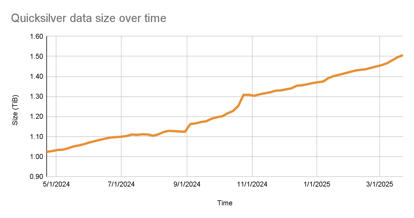
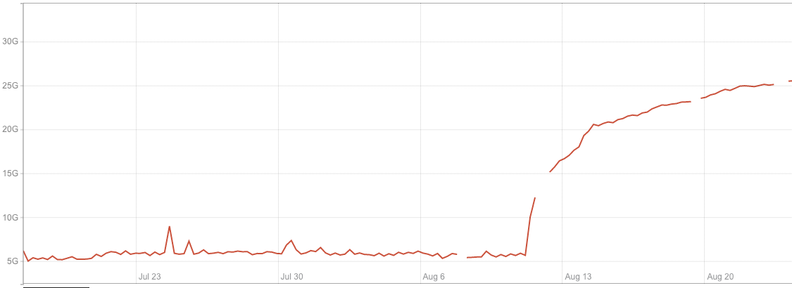
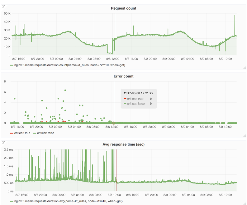
^{The size of the Quicksilver database has grown by 50% to about 1.6 TB in the past year}

What we talked about previously

Part one of the story explained how Quicksilver V1 stored all key-value pairs on each server all around the world. It was a very simple and fast design, it worked very well, and it was a great way to get started. But over time, it turned out to not scale well from a disk space perspective.

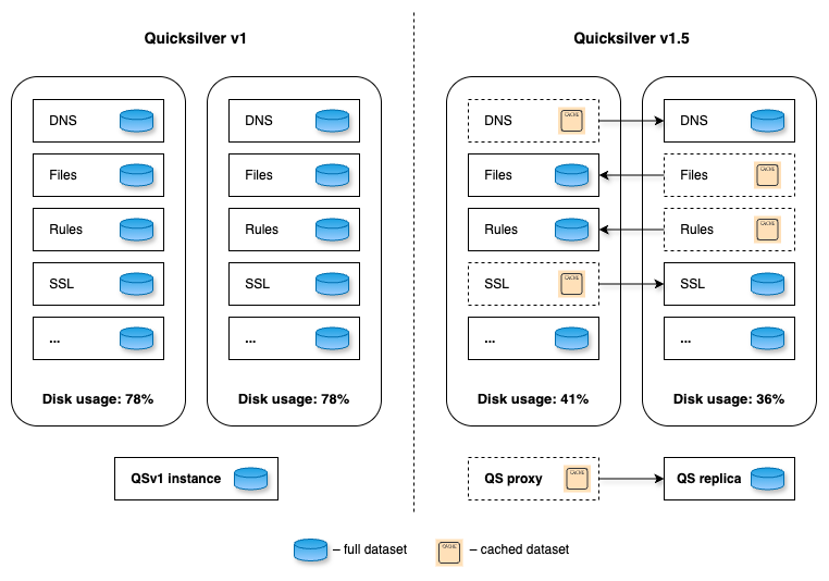
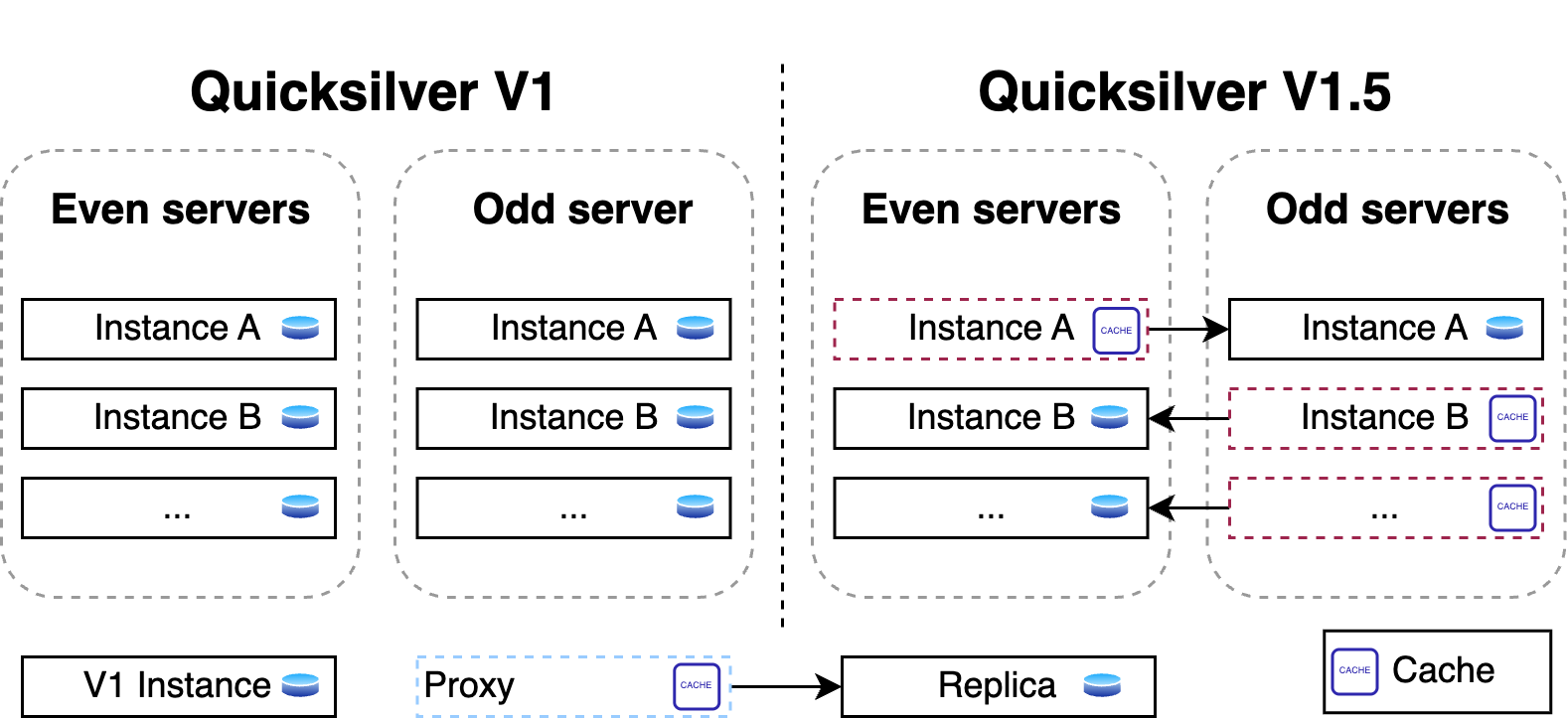
The problem was that disk space was running out so fast that there was not enough time to design and implement a fully scalable version of Quicksilver. Therefore, Quicksilver V1.5 was created first. It halved the disk space used on each server compared to V1.

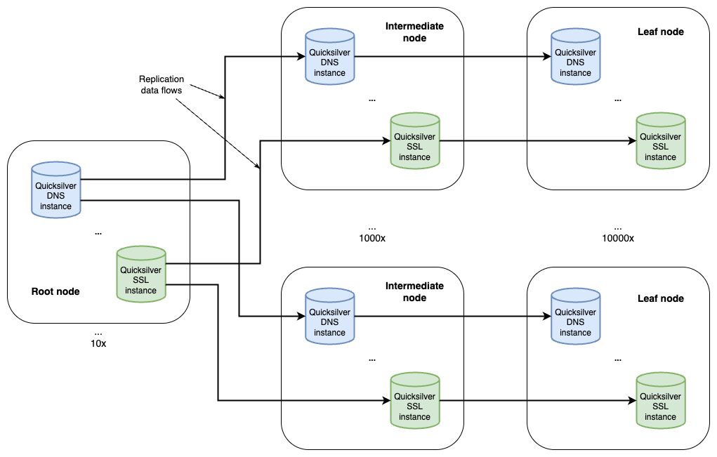
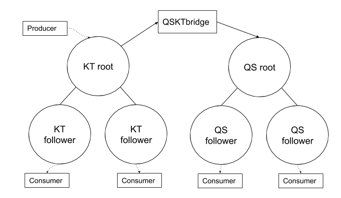
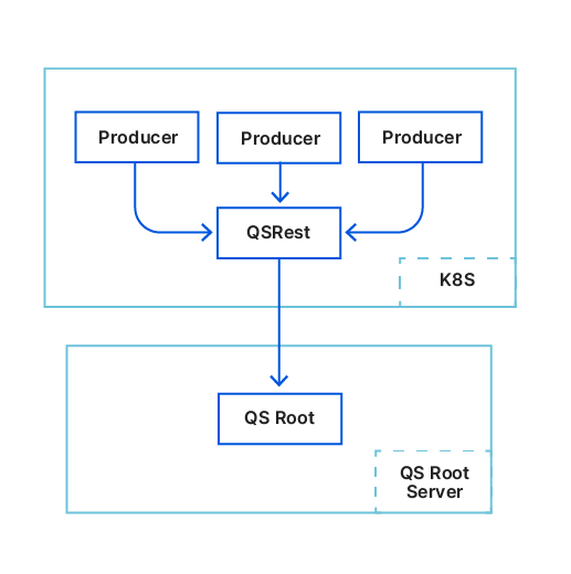
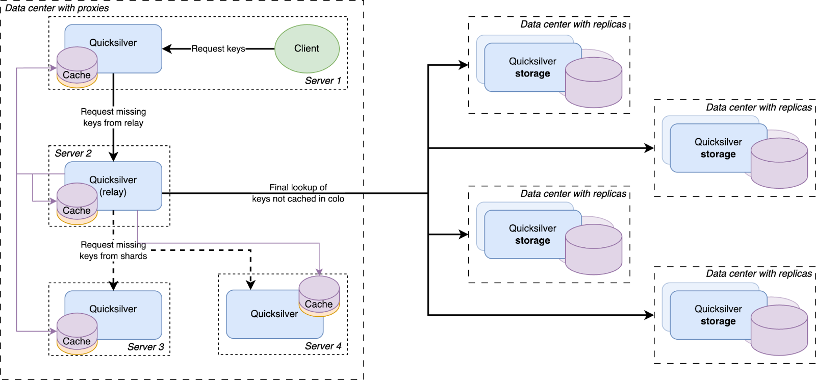
For this, a new proxy mode was introduced for Quicksilver. In this mode, Quicksilver does not contain the full dataset anymore, but only contains a cache. All cache misses are looked up on another server that runs Quicksilver with a full dataset. Each server runs about ten separate instances of Quicksilver, and all have different databases with different sets of key-values. We call Quicksilver instances with the full data set replicas.

For Quicksilver V1.5, half of those instances on a particular server would run Quicksilver in proxy mode, and therefore would not have the full dataset anymore. The other half would run in replica mode. This worked well for a time, but it was not the final solution.

Building this intermediate solution had the added benefit of allowing the team to gain experience running an even more distributed version of Quicksilver.

The problem

There were a few reasons why Quicksilver V1.5 was not fully scalable.

First, the size of the separate instances were not very stable. The key-space is owned by the teams that use Quicksilver, not by the Quicksilver team, and the way those teams use Quicksilver changes frequently. Furthermore, while most instances grow in size over time, some instances have actually gotten smaller, such as when the use of Quicksilver is optimised by teams. The result of this is that the split of instances that was well-balanced at the start, quickly became unbalanced.

Second, the analyses that were done to estimate how much of the key space would need to be in cache on each server assumed that taking all keys that were accessed in a three-day period would represent a good enough cache. This assumption turned out to be wildly off. This analysis estimated that we needed about 20% of the key space in cache, which turned out to not be entirely accurate. Whereas most instances did have a good cache hit rate, with 20% or less of the key space in cache, some instances turned out to need a much higher percentage.

The main issue, however, was that reducing the disk space used by Quicksilver on our network by as much as 40% does not actually make it more scalable. The number of key-values that are stored in Quicksilver keeps growing. It only took about two years before disk space was running low again.

The solution

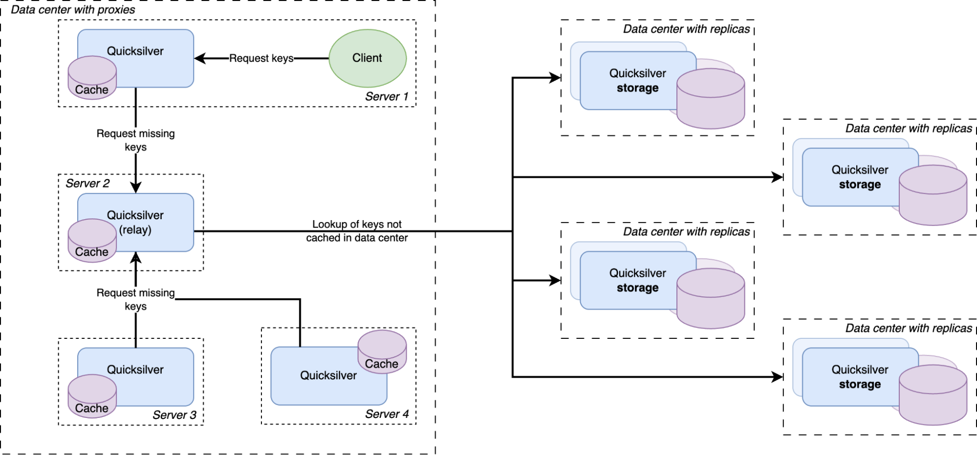
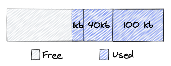
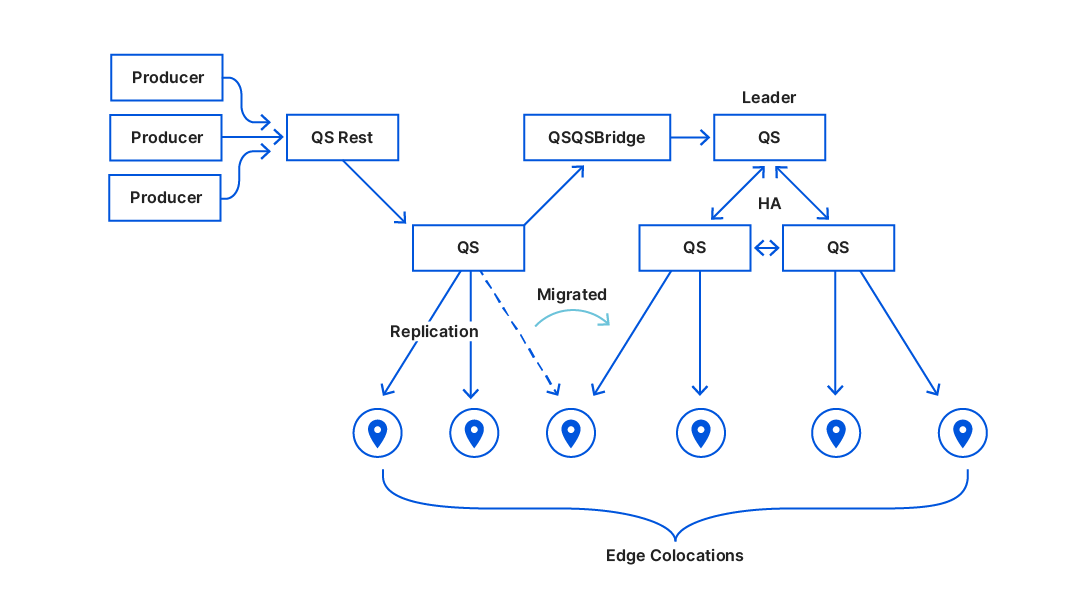
^{Except for a handful of special storage servers, Quicksilver does not contain the full dataset anymore, but only cache. Any cache misses will be looked up in replicas on our storage servers, which do have the full dataset.}

The solution to the scalability problem was brought on by a new insight. As it turns out, numerous key-values were actually almost never used. We call these cold keys. There are different reasons for these cold keys: some of them were old and not well cleaned up, some were used only in certain regions or in certain data centers, and some were not used for a very long time or maybe not at all (a domain name that is never looked up for example or a script that was uploaded but never used).

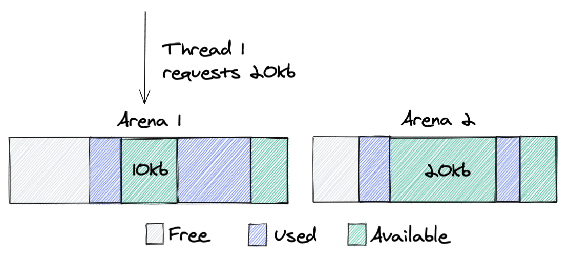
At first, the team had been considering solving our scalability problem by splitting up the entire dataset into shards and distributing those across the servers in the different data centers. But sharding the full dataset adds a lot of complexity, corner cases, and unknowns. Sharding also does not optimize for data locality. For example, if the key-space is split into 4 shards and each server gets one shard, that server can only serve 25% of the requested keys from its local database. The cold keys would also still be contained in those shards and would take up disk space unnecessarily.

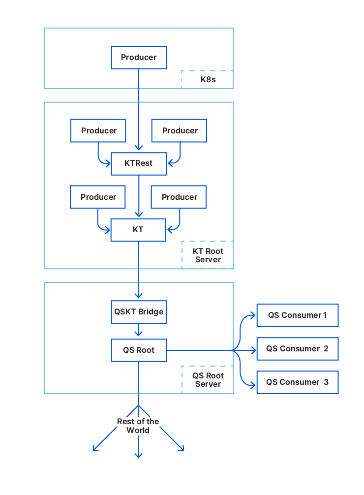
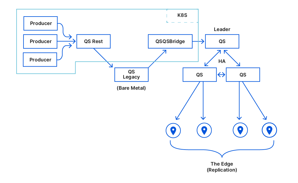
Another data structure that is much better at data locality and explicitly avoids storing keys that are never used is a cache. So it was decided that only a handful of servers with large disks would maintain the full data set, and all other servers would only have a cache. This was an obvious evolution from Quicksilver V1.5. Caching was already being done on a smaller scale, so all the components were already available. The caching proxies and the inter-data center discovery mechanisms were already in place. They had been used since 2021 and were therefore thoroughly battle tested. However, one more component needed to be added.

There was a concern that having all instances on all servers connect to a handful of storage nodes with replicas would overload them with too many connections. So a Quicksilver relay was added. For each instance, a few servers would be elected within each data center on which Quicksilver would run in relay mode. The relays would maintain the connections to the replicas on the storage nodes. All proxies inside a data center would discover those relays and all cache misses would be relayed through them to the replicas.

This new architecture worked very well. The cache hit rates still needed some improvement, however.

Prefetching the future

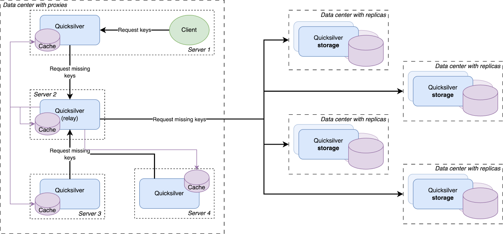
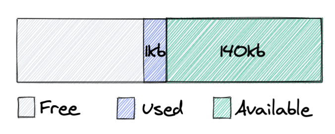
^{Every resolved cache miss is prefetched by all servers in the data center}

We had a hypothesis that prefetching all keys that were cache misses on the other servers inside the same data center would improve the cache hit rate. So an analysis was done, and it indeed showed that every key that was a cache miss on one server in a data center had a very high probability of also being a cache miss on another server in the same data center sometime in the near future. Therefore, a mechanism was built that distributed all resolved cache misses on relays to all other servers.

All cache misses in a data center are resolved by requesting them from a relay, which subsequently forwards the requests to one of the replicas on the storage nodes. Therefore, the prefetching mechanism was implemented by making relays publish a stream of all resolved cache misses, to which all Quicksilver proxies in the same data center subscribe. The resulting key-values were then added to the proxy local caches.

This strategy is called reactive prefetching, because it fills caches only with the key-values that directly resulted from cache misses inside the same data center. Those prefetches are a reaction to the cache misses. Another way of prefetching is called predictive prefetching, in which an algorithm tries to predict which keys that have not yet been requested will be requested in the near future. A few approaches for making these predictions were tried, but they did not result in any improvement, and so this idea was abandoned.

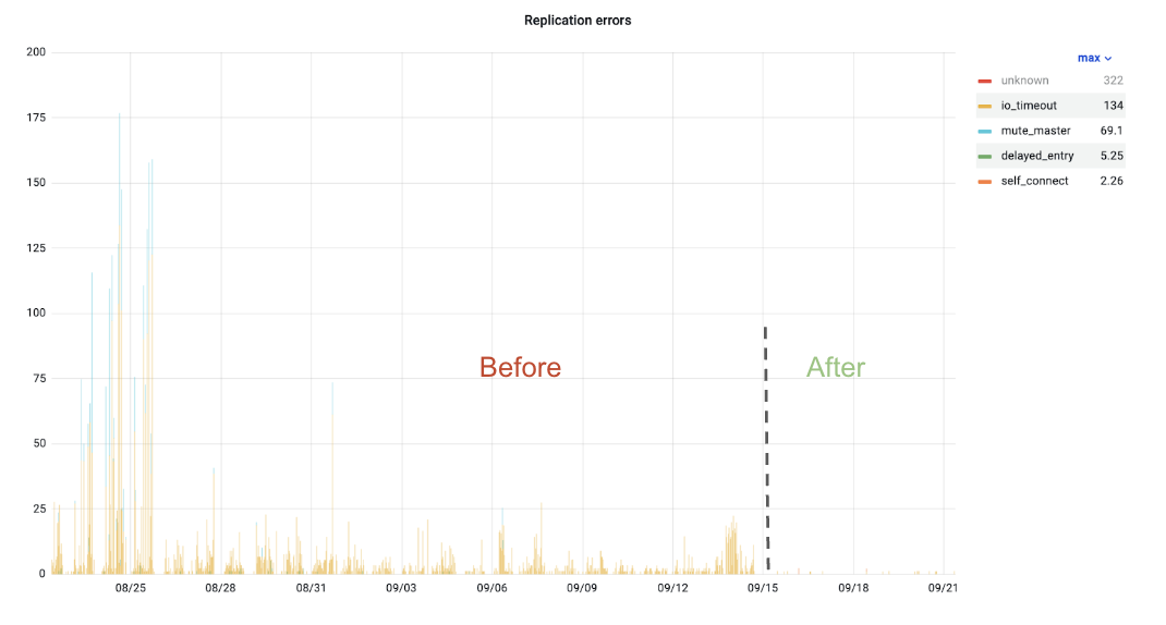
With the prefetching enabled, cache hit rates went up to about 99.9% for the worst performing instance. This was the goal that we were trying to reach. But while rolling this out to more of our network, it turned out that there was one team that needed an even higher cache hit rate, because the tail latencies they were seeing with this new architecture were too high.

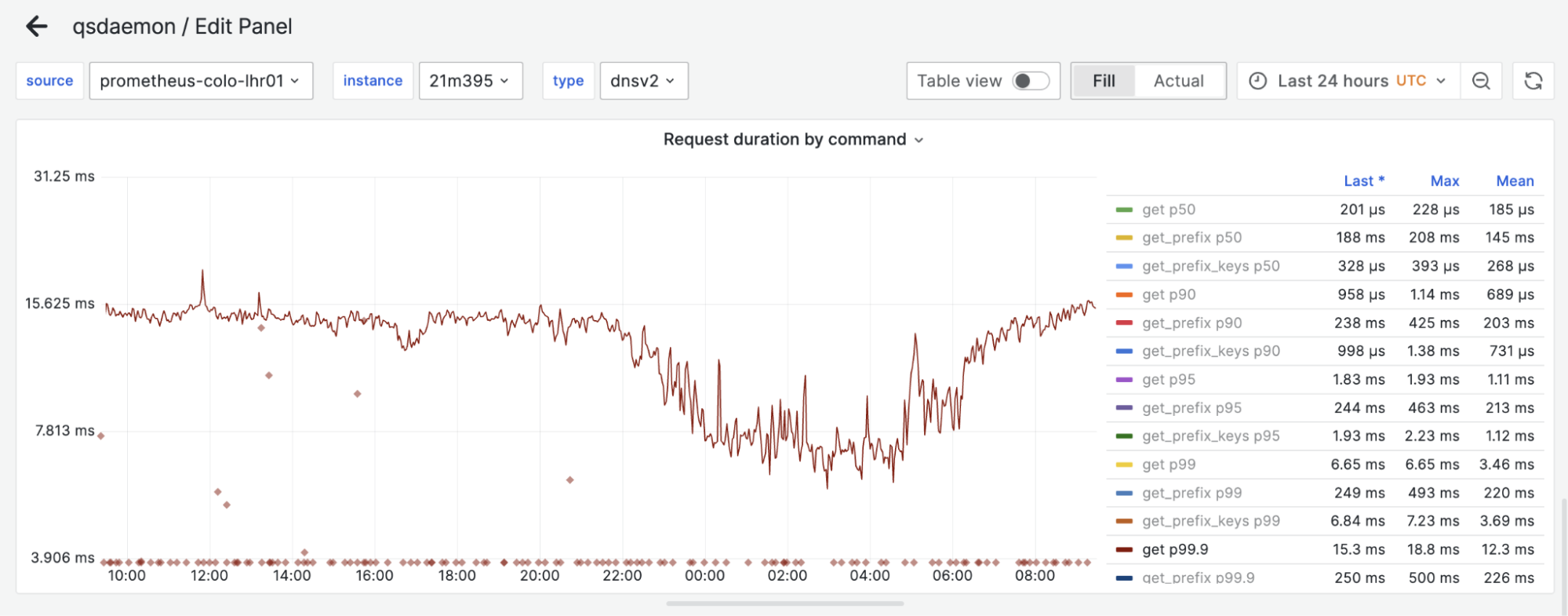
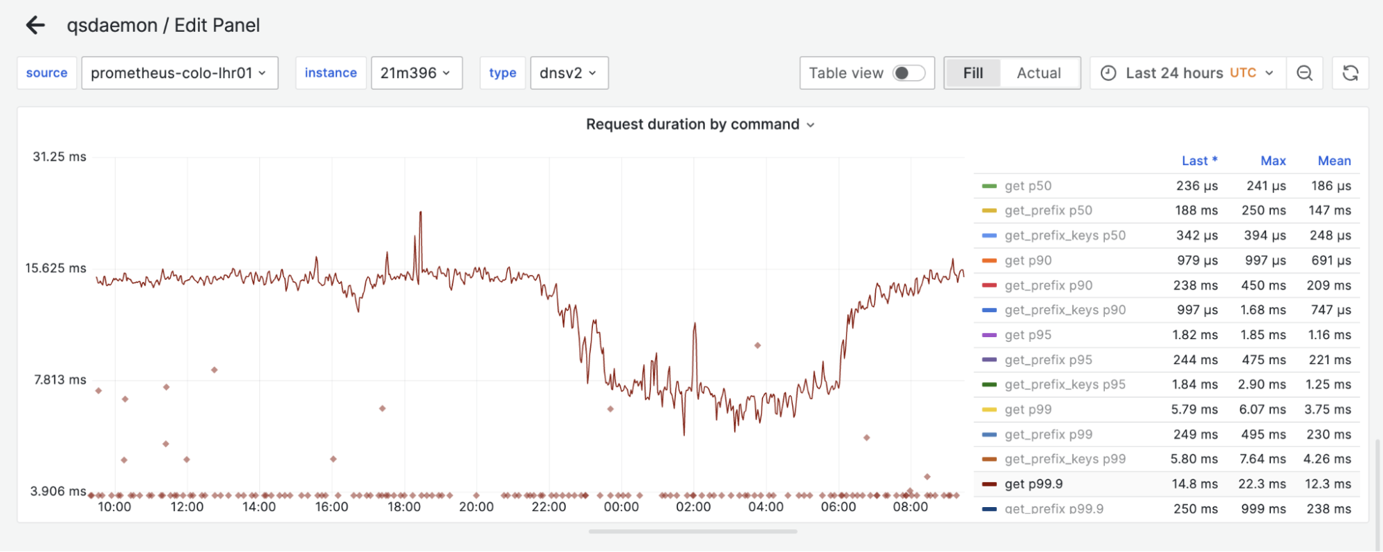
This team was using a Quicksilver instance called dnsv2. This is a very latency sensitive instance, because it is the one from which DNS queries are served. Some of the DNS queries under the hood need multiple queries to Quicksilver, so any added latency to Quicksilver multiplies for them. This is why it was decided that one more improvement to the Quicksilver cache was needed.

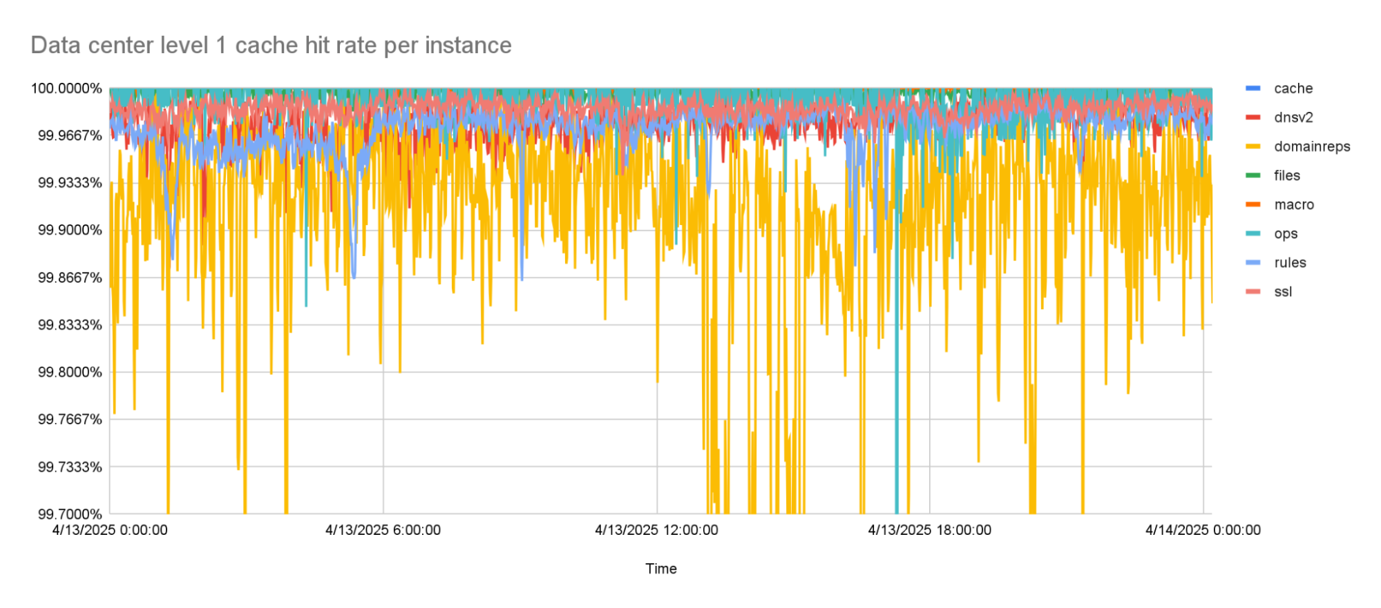
^{The level 1 cache hit-rate is 99.9% or higher, on average.}

Back to the sharding

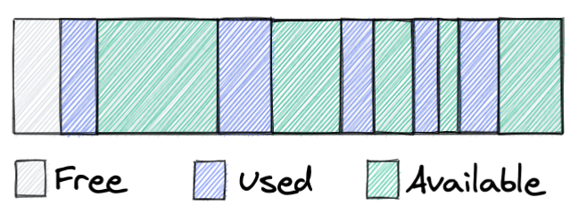
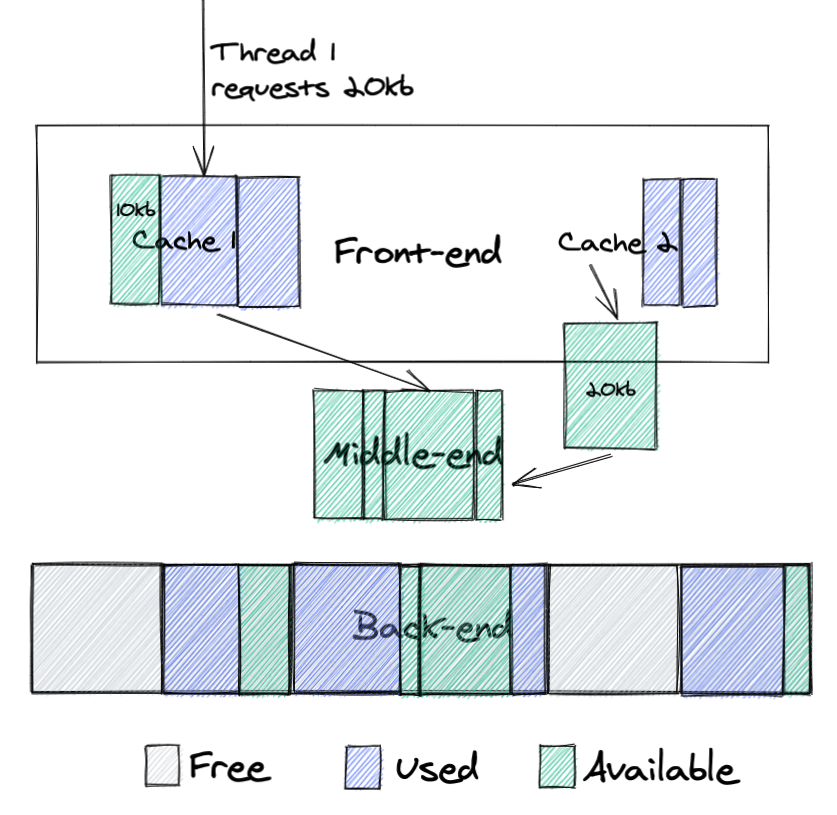
^{Before going to a replica in another data center, a cache miss is first looked up in a data center-wide sharded cache}

The instance on which higher cache hit rates were required was also the instance on which the cache performed the worst. The cache works with a retention time, defined as the number of days a key-value is kept in cache after it was last accessed, after which it is evicted from the cache. An analysis of the cache showed that this instance needed a much longer retention time. But, a higher retention time also causes the cache to take up more disk space — space that was not available.

However, while running Quicksilver V1.5, we had already noticed the pattern that caches generally performed much better in smaller data centers as compared to larger ones. This sparked the hypothesis that led to the final improvement.

It turns out that smaller data centers, with fewer servers, generally needed less disk space for their cache. Vice versa, the more servers there are in a data center, the larger the Quicksilver cache needs to be. This is easily explained by the fact that larger data centers generally serve larger populations, and therefore have a larger diversity of requests. More servers also means more total disk space available inside the data center. To be able to make use of this pattern the concept of sharding was reintroduced.

Our key space was split up into multiple shards. Each server in a data center was assigned one of the shards. Instead of those shards containing the full dataset for their part of the key space, they contain a cache for it. Those cache shards are populated by all cache misses inside the data center. This all forms a data center-wide cache that is distributed using sharding.

The data locality issue that sharding the full dataset has, as described above, is solved by keeping the local per-server caches as well. The sharded cache is in addition to the local caches. All servers in a data center contain both their local cache and a cache for one physical shard of the sharded cache. Therefore, each requested key is first looked up in the server’s local cache, after that the data center-wide sharded cache is queried, and finally if both caches miss the requested key, it is looked up on one of the storage nodes.

The key space is split up into separate shards by first dividing hashes of the keys by range into 1024 logical shards. Those logical shards are then divided up into physical shards, again by range. Each server gets one physical shard assigned by repeating the same process on the server hostname.

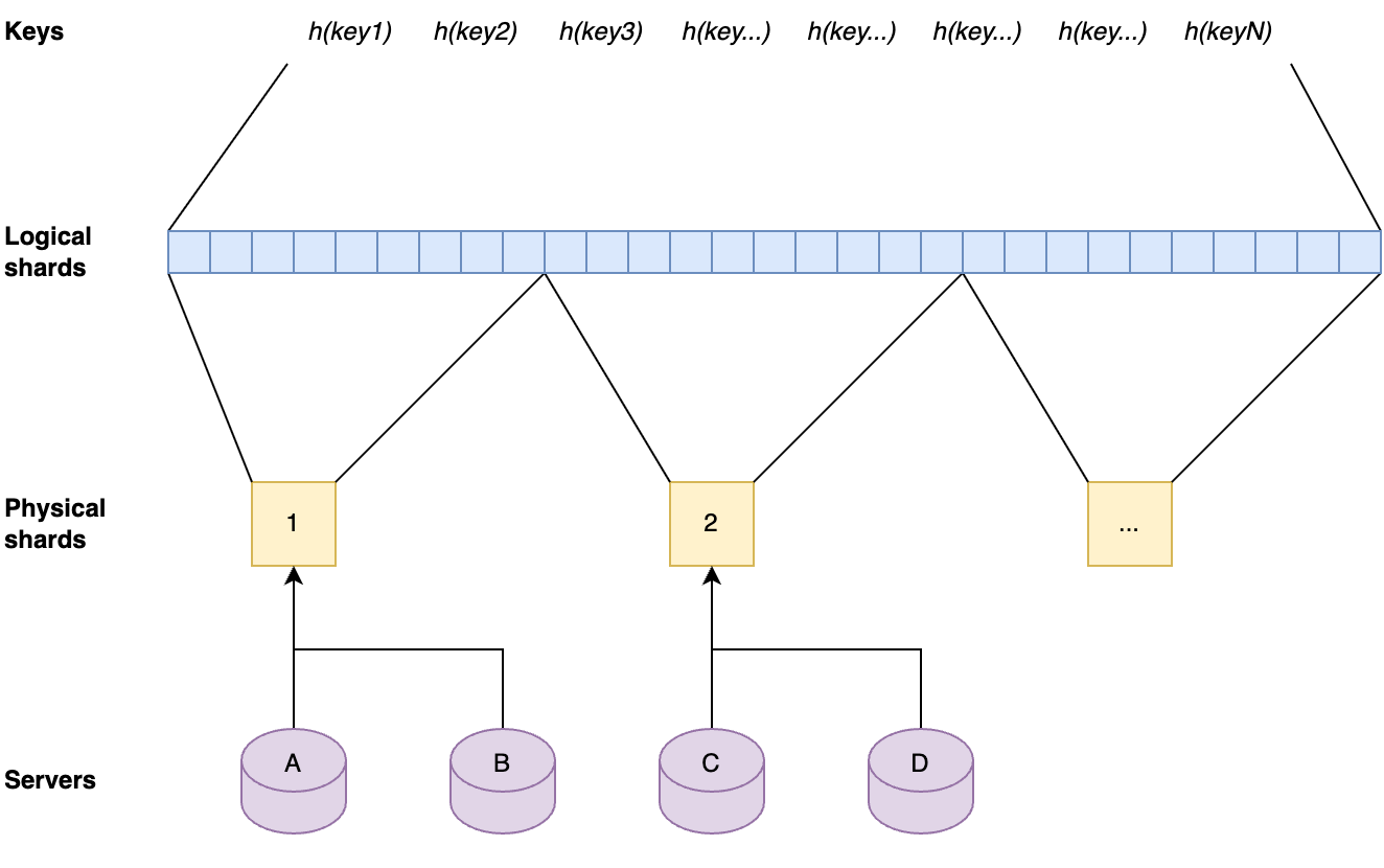
^{Each server contains one physical shard. A physical shard contains a range of logical shards. A local shard contains a range of the ordered set that result from hashing all keys.}

This approach has the advantage that the sharding factor can be scaled up by factors of two without the need for copying caches to other servers. When the sharding factor is increased in this way, the servers will automatically get a new physical shard assigned that contains a subset of the key space that the previous physical shard on that server contained. After this has happened, their cache will contain supersets of the needed cache. The key-values that are not needed anymore will be evicted over time.

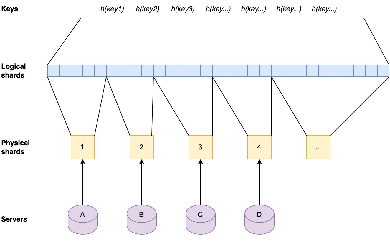
^{When the number of physical shards are doubled the servers will automatically get new physical shards that are subsets of their previous physical shards, therefore still have the relevant key-values in cache.}

This approach means that the sharded caches can easily be scaled up when needed as the number of keys that are in Quicksilver grows, and without any need for relocating data. Also, shards are well-balanced due to the fact that they contain uniform random subsets of a very large key-space.

Adding new key-values to the physical cache shards piggybacks on the prefetching mechanism, which already distributes all resolved cache misses to all servers in a data center. The keys that are part of the key space for a physical shard on a particular server are just kept longer in cache than the keys that are not part of that physical shard.

Another reason why a sharded cache is simpler than sharding the full key-space is that it is possible to cut some corners with a cache. For instance, looking up older versions of key-values (as used for multiversion concurrency control) is not supported on cache shards. As explained in an earlier blog post, this is needed for consistency when looking up key-values on different servers, when that server has a newer version of the database. It is not needed in the cache shards, because lookups can always fall back to the storage nodes when the right version is not available.

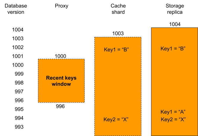
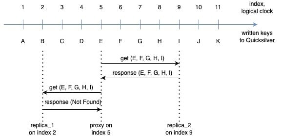
^{Proxies have a recent keys window that contains all recently written key-values. A cache shard only has its cached key-values. Storage replicas contain all key-values and on top of that they contain multiple versions for recently written key-values. When the proxy, that has database version 1000, has a cache miss for}^key1^{it can be seen that the version of that key on the cache shard was written at database version 1002 and therefore is too new. This means that it is not consistent with the proxy’s database version. This is why the relay will fetch that key from a replica instead, which can return the earlier consistent version. In contrast,}^key2^{on the cache shard can be used, because it was written at index 994, well below the database version of the proxy.}

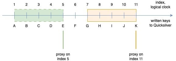
There is only one very specific corner case in which a key-value on a cache shard cannot be used. This happens when the key-value in the cache shard was written at a more recent database version than the version of the proxy database at that time. This would mean that the key-value probably has a different value than it had at the correct version. Because, in general, the cache shard and the proxy database versions are very close to each other, and this only happens for key-values that were written in between those two database versions, this happens very rarely. As such, deferring the lookup to storage nodes has no noticeable effect on the cache hit rate.

Tiered Storage

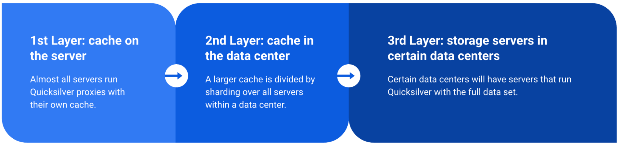
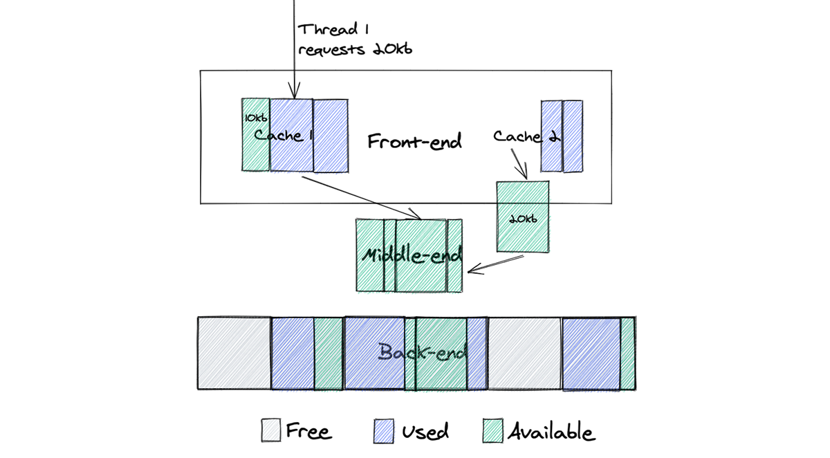
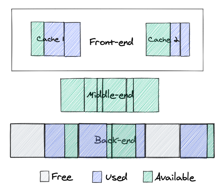
To summarize, Quicksilver V2 has three levels of storage.

Level 1: The local cache on each server that contains the key-values that have most recently been accessed.
Level 2: The data center wide sharded cache that contains key-values that haven’t been accessed in a while, but do have been accessed.
Level 3: The replicas on the storage nodes that contain the full dataset, which live on a handful of storage nodes and are only queried for the cold keys.

The results

The percentage of keys that can be resolved within a data center improved significantly by adding the second caching layer. The worst performing instance has a cache hit rate higher than 99.99%. All other instances have a cache hit rate that is higher than 99.999%.

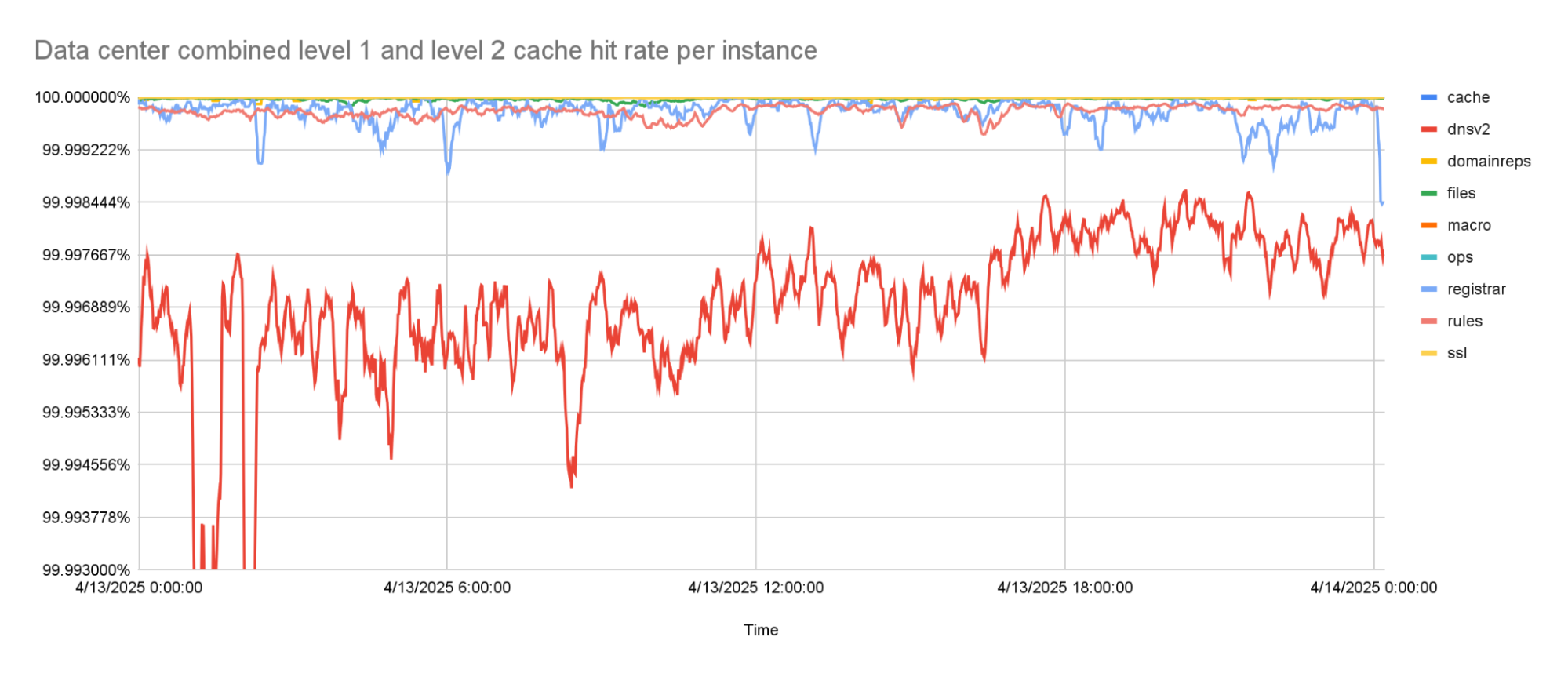
^{The combined level 1 and level 2 cache hit-rate is 99.99% or higher for the worst caching instance.}

Final notes

It took the team quite a few years to go from the old Quicksilver V1, where all data was stored on each server to the tiered caching Quicksilver V2, where all but a handful of servers only have cache. We faced many challenges, including migrating hundreds of thousands of live databases without interruptions, while serving billions of requests per second. A lot of code changes were rolled out, with the result that Quicksilver now has a significantly different architecture. All of this was done transparently to our customers. It was all done iteratively, always learning from the previous step before taking the next one. And always making sure that, if at all possible, all changes are easy to revert. These are important strategies for migrating complex systems safely.

If you like these kinds of stories, keep an eye out for more development stories on our blog. And if you are enthusiastic about solving these kinds of problems, we are hiring for multiple types of roles across the organization

Thank you

And finally, a big thanks to the rest of the Quicksilver team, because we all do this together: Aleksandr Matveev, Aleksei Surikov, Alex Dzyoba, Alexandra (Modi) Stana-Palade, Francois Stiennon, Geoffrey Plouviez, Ilya Polyakovskiy, Manzur Mukhitdinov, Volodymyr Dorokhov.

Quicksilver v2: evolution of a globally distributed key-value store (Part 1)

2025-07-10 Anton Dort-Golts

Post Syndicated from Anton Dort-Golts original https://blog.cloudflare.com/quicksilver-v2-evolution-of-a-globally-distributed-key-value-store-part-1/

Quicksilver is a key-value store developed internally by Cloudflare to enable fast global replication and low-latency access on a planet scale. It was initially designed to be a global distribution system for configurations, but over time it gained popularity and became the foundational storage system for many products in Cloudflare.

A previous post described how we moved Quicksilver to production and started replicating on all machines across our global network. That is what we called Quicksilver v1: each server has a full copy of the data and updates it through asynchronous replication. The design served us well for some time. However, as our business grew with an ever-expanding data center footprint and a growing dataset, it became more and more expensive to store everything everywhere.

We realized that storing the full dataset on every server is inefficient. Due to the uniform design, data accessed in one region or data center is replicated globally, even if it’s never accessed elsewhere. This leads to wasted disk space. We decided to introduce a more efficient system with two new server roles: replica, which stores the full dataset and proxy, which acts as a persistent cache, evicting unused key-value pairs to free up some disk space. We call this design Quicksilver v1.5 – an interim step towards a more sophisticated and scalable system.

To understand how those two roles helped us reduce disk space usage, we first need to share some background on our setup and introduce some terminology. Cloudflare is architected in a way where we have a few hyperscale core data centers that form our control plane, and many smaller data centers distributed across the globe where resources are more constrained. Quicksilver has dozens of servers in the core data centers with terabytes of storage called root nodes. In the smaller data centers, though, things are different. A typical data center has two types of nodes: intermediate nodes and leaf nodes. Intermediate servers replicate data either from the other intermediate nodes or directly from the root nodes. Leaf nodes serve end user traffic, and receive updates from intermediate servers, effectively being leaves of a replication tree. Disk capacity varies significantly between node types. While root nodes aren’t facing an imminent disk space bottleneck, it’s a definite concern for leaf nodes.

Every server – whether it’s a root, intermediate, or leaf – hosts 10 Quicksilver instances. These are independent databases, each used by specific Cloudflare services or products such as the DNS, CDN or WAF.

^{Figure 1. Global Quicksilver}

Let’s consider the role distribution. Instead of hosting ten full datasets on every machine within a data center, what if we deploy only a few replicas in each? The remaining servers would be proxies, maintaining a persistent cache of hot keys and querying replicas for any cache misses.

^{Figure 2. Role allocation for different Quicksilver instances}

Data centers across our network are very different in size, ranging from hundreds of servers to a single rack with just a few servers. To ensure every data center has at least one replica, the simplest initial step is an even split: on each server, place five replicas of some instances and five proxies for others. The change immediately frees up disk space, as the cached hot dataset on a proxy should be smaller than a full replica. While it doesn’t remove the bottleneck entirely, it could, in theory, lead to an up to 50% reduction in disk space usage. More importantly, it lays the foundation for a new distributed design of Quicksilver, where queries can be served by multiple machines in a data center, paving the way for further horizontal scaling. Additionally, an iterative approach helps to battle-proof the code changes earlier.

Can it even work?

Before committing to building Quicksilver v1.5, we wanted to be sure that the proxy/replica design would actually work for our workload. If proxies needed to cache the entire dataset for good performance, then it would be a dead end, offering no potential disk space benefits. To assess this, we built a data pipeline which pushes accessed keys from all across our network to ClickHouse. This allowed us to estimate typical sizes of working sets. Our analysis revealed that:

in large data centers approximately, 20% of the keyspace was in use
in small data centers this number dropped to just about 1%

These findings gave us confidence that the caching approach should work, though it wouldn’t be without its challenges.

Persistent caching

When talking about caches, the first thing that comes to mind is an in-memory cache. However, this cannot work for Quicksilver for two main reasons: memory usage and the “cold cache” problem.

Indeed, with billions of stored keys, even a fraction of them would lead to an unmanageable increase in memory usage. System restarts should not affect performance, which means that cache data must be preserved somewhere anyway. So we decided to make the cache persistent and store it in the same way as full datasets: in our embedded RocksDB. Thus, cached keys normally sit on disk and can be retrieved on-demand with low memory footprint.

When a key cannot be found in the proxy’s cache, we request it from a replica using our internal distributed key-value protocol, and put it into a local cache after processing.

Evictions are based on RocksDB compaction filters. Compaction filters allow defining custom logic executed in background RocksDB threads responsible for compacting files on disk. Each key-value pair is processed with a filter on a regular basis, evicting least recently used data from the disk when available disk space drops below a certain threshold called a soft limit. To track keys accessed on disk, we have an LRU-like in-memory data structure, which is passed to the compaction filter to set last access date in key metadata and inform potential evictions.

However, with some specific workloads there is still a chance that evictions will not keep up with disk space growth, and for this scenario we have a hard limit: when available disk space drops below a critical threshold, we temporarily stop adding new keys to the cache. This hurts performance, but it acts as a safeguard, ensuring our proxies remain stable and don’t overflow under a massive surge of requests.

Consistency and asynchronous replication

Quicksilver has, from the start, provided sequential consistency to clients: if key A was written before B, it’s not possible to read B and not A. We are committed to maintaining this guarantee in the new design. We have experienced Hyrum’s Law first hand, with Quicksilver being so widely adopted across the company that every property we introduced in earlier versions is now relied upon by other teams. This means that changing behaviour would inevitably break existing functionality and introduce bugs.

However, there is one thing standing in our way: asynchronous replication. Quicksilver replication is asynchronous mainly because machines in different parts of the world replicate at different speeds, and we don’t want a single server to slow down the entire tree. But it turns out in a proxy-replica design, independent replication progress can result in non-monotonic reads!

Consider the following scenario: a client sequentially writes keys A, B, C, .. K one after another to the Quicksilver root node. These keys are asynchronously replicated through data centers across our network with varying latency. Imagine we have a proxy on index 5, which has observed keys from A to E, and two replicas:

replica_1 is at index 2 (slightly behind the proxy), having only received A and B
replica_2 at index 9, which is slightly ahead due to a faster replication path and has received all keys from A to I

^{Figure 3. Asynchronous replication in QSv1.5}

Now, a client performs two successive requests on a proxy, each time reading the keys E, F, G, H and I. For simplicity, we assume these keys are not cacheable (for example, due to low disk space). The proxy’s first remote request is routed to replica_2, which already has all keys and responds back with values. To prevent hot spots in a data center, we load balance requests from proxies, and the next one lands on replica_1, which hasn’t received any of the requested keys yet, and responds with a “not found” error.

So, which result is correct?

The correct behavior here is that of Quicksilver v1, which we aim to preserve. If the server on replication index 5 were a replica instead of a proxy, it would have seen updates for keys A through E inclusive, resulting in E being the only key in both replies, while all other keys cannot be found yet. Which means responses from both replica_1 and replica_2 are wrong!

Therefore, to maintain previous guarantees and API backwards compatibility, Quicksilver v1.5 must address two crucial consistency problems: cases where the replica is ahead of the proxy, and conversely, where it lags behind. For now let’s focus on the case where a proxy lags behind a replica.

Multiversion concurrency control

In our example, replica_2 responds to a request from a proxy “from the past”. We cannot use any locks for synchronizing two servers, as it would introduce undesirable delays to the replication tree, defeating the purpose of asynchronous replication. The only option is for replicas to maintain a history of recent updates. This naturally leads us to implementing multiversion concurrency control (MVCC), a popular database mechanism for tracking changes in a non-blocking fashion, where for any key we can keep multiple versions of its values for different points in time.

With MVCC, we no longer overwrite the latest value of a key in the default column family for every update. Instead, we introduced a new MVCC column family in RocksDB, where all updates are stored with a corresponding replication index. Lookup for a key at some index in the past goes as follows:

First we search in the default column family. If a key is found and the write timestamp is not greater than the index of a requesting proxy, we can use it straight away.
Otherwise, we begin scanning the MVCC column family, where keys have unique suffixes based on latest timestamps for which they are still valid.

In the example above, replica_2 has MVCC enabled and has keys A@1 .. K@11 in its default column family. The MVCC is initially empty, because no keys have been overwritten yet. When it receives a request for, say, key H with target index 5, it first makes a lookup in a default column family and finds the given key, but its timestamp is 8, which means this version should not be visible to the proxy yet. It then scans the MVCC, finds no matching previous versions and responds with “not found” to the proxy. Should key H be updated twice at indexes 4 and 8, we would have placed the initial version into MVCC before overwriting it in the default column family, and the proxy would receive the first version in response.

If a key E is requested at index 5, replica_2 can find it quickly in the default column family and return it back to the proxy. There is no need to read from MVCC, as the timestamp of the latest version (5) satisfies the request.

Another corner case to consider is deletions. When a key is deleted and then re-written, we need to explicitly mark the period of removal in MVCC. For that we’ve implemented tombstones – a special value format for absent keys.

Finally, we need to make sure that key history is not growing uncontrollably, using up all of the disk space available. Luckily we don’t actually need to record history for a long period of time, it just needs to cover the maximum replication index difference between any two machines. And in practice, a two-hour interval turned out to be way more than enough, while adding only about 500 MB of extra disk space usage. All records in the MVCC column family older than two hours are garbage collected, and for that again we use custom RocksDB compaction filters.

Sliding window

Now we know how to deal with proxies lagging behind replicas. But what about the opposite case, when a proxy is ahead of replicas?

The simplest solution is for replicas to not serve requests with a target index higher than its own. After all, it cannot know about keys from the future, whether they will be added, updated, or removed. In fact, our first implementation just returned an error when the proxy was ahead, as we expected it to happen quite infrequently. But after rolling out gradually to a few data centers, our metrics made it clear that the approach was not going to work.

This led us to analyze which keys are affected by this kind of replication asymmetry. It’s definitely not keys added or updated a long time ago, because replicas would already have the changes replicated. The only problematic keys are those updated very recently, which the proxy already knows about, but the replica does not.

With this insight, we realized that the issue should be solved on the proxies rather than on the replica side. By preserving all recent updates locally, the proxy can avoid querying the replica. This became known as the sliding window approach.

The sliding window retains all recent updates written in a short, rolling timeframe. Unlike cached keys, items in the window cannot be evicted until they move outside of the window. Internally, the sliding window is defined by lower and upper boundary pointers. These are kept in memory, and can easily be restored after a reload from the current database index and the pre-configured window size.

^{Figure 4. The sliding window shifts when replication updates arrive}

When a new update event arrives from the replication layer we add it to the sliding window by moving both the upper and lower boundary one position higher. Thereby, we maintain the fixed size of the window. Keys written before the lower bound can be evicted by the compaction filter, which is aware of current sliding window boundaries.

Negative lookups

Another problem arising with our distributed replica-proxy design is negative lookups – requests for keys which don’t exist in the database. Interestingly, in our workloads we see about ten times more negative lookups than positive ones!

But why is it a problem? Unfortunately, each negative lookup will be a cache miss on a proxy, requiring a request to a replica. Given the volume of requests and proportion of such lookups, it would be a disaster for performance, with overloaded replicas, overused data center networks, and massive latency degradation. We needed a fast and efficient approach to identifying non-existing keys directly at the proxy level.

In v1, negative lookups are the quickest type of requests. We rely on a special probabilistic data structure – Bloom filters – used in RocksDB to determine if the requested key might belong to a certain data file containing a range of sorted keys (called Sorted Sequence Table or SST) or definitely not. 99% of the time, negative lookups are served using only this in-memory data structure, avoiding the need for disk I/O.

One approach we considered for proxies was to cache negative lookups. Two problems immediately arise:

How big is the keyspace of negative lookups? In theory, it’s infinite, but the real size was unclear. We can store it in our cache only if it is small enough.
Cached negative lookups would no longer be served by the fast Bloom filters. We have row and block caches in RocksDB, but the hit rate is nowhere near the filters for SSTs, which means negative lookups would end up going to disk more often.

These turned out to be dealbreakers: not only was the negative keyspace vast, greatly exceeding the actual keyspace (by a thousand times for some instances!), but clients also need lookups to be really fast, ideally served from memory.

In pursuit of probabilistic data structures which could give us a dynamic compact representation of a full keyspace on proxies, we spent some time exploring Cuckoo filters. Unfortunately, with 5 billion keys it takes about 18 GB to have a false positive rate similar to Bloom filters (which only require 6 GB). And this is not only about wasted disk space — to be fast we have to keep it all in memory too!

Clearly some other solution was needed.

Finally, we decided to implement key and value separation, storing all keys on proxies, but persisting values only for cached keys. Evicting a key from the cache actually results in the removal of its value.

But wait, don’t the keys, even stripped of values, take a lot of space? Well, yes and no.

The total size of pure keys in Quicksilver is approximately 11 times smaller than the full dataset. Of course, it’s larger than any representation by probabilistic data structure, but there are some very desirable properties to such a solution. Firstly, we continue to enjoy fast Bloom filter lookups in RocksDB. Another benefit is that it unlocks some cool optimizations for range queries in a distributed context.

We may revisit it one day, but so far it has worked great for us.

Discovery mechanism

Having solved all of the above challenges, one bit remained to be sorted out to make distributed query execution work: how can proxies discover replicas?

Within the local data center it is fairly easy. Each one runs its own consul cluster, where machines are registered as services. Consul is well integrated with our internal DNS resolvers, and with a single DNS request, we can get the names of all replicas running in a data center, which proxies can directly connect to.

However, data centers vary in size, servers are constantly added and removed, and having only local discovery would not be enough for the system to work reliably. Proxies also need to find replicas in other nearby data centers.

We had previously encountered a similar problem with our replication layer. Initially, the replication topology was statically defined in a configuration and distributed to all servers, such that they know from which sources they should replicate. While simple, this approach was quite fragile and tedious to operate. It led to a rigid replication tree with suboptimal overall performance, unable to adapt to network changes.

Our solution to this problem was the Network Oracle – a special overlay network based on a gossip protocol and consisting of intermediate nodes in our data centers. Each member of this overlay constantly exchanges status and metainformation with other nodes, which helps us see active members in near-real time. Each member runs network probes measuring round-trip time to its peers, making it easy to find closest (in terms of RTT) active intermediate nodes to form a low-latency replication tree. Introducing the Network Oracle was a major improvement: we no longer needed to reconfigure the topology, watch intermediate nodes or entire data centers go down, or investigate frequent replication issues. Replication is now a completely self-organized and self-healing dynamic system.

Naturally, we decided to reuse the Network Oracle for our discovery mechanism. It consists of two subproblems: data center discovery and specific service lookup. We use the Network Oracle to find the closest data centers. Adding all machines running Quicksilver to the same overlay would be inefficient because of significant increase of network traffic and message delivery times. Instead, we use intermediate nodes as sources of network proximity information for the leaf nodes. Knowing which data centers are nearby, we can directly send DNS queries there to resolve specific services – Quicksilver replicas in this case.

Proxies maintain a pool of connections to active replicas and distribute requests among them to smooth out the load and avoid hotspots in a data center. Proxies also have a health-tracking mechanism, monitoring the state of connections and errors coming from replicas, and temporarily deprioritizing or isolating potentially faulty ones.

^{Figure 5. Internal replica request errors}

To demonstrate its efficiency, we graphed errors coming from replica requests, which showed that such errors almost disappeared after introducing the new discovery system.

Results

Our objective with Quicksilver v1.5 was simple: gain some disk space without losing request latency, because clients rely heavily on us being fast. While the replica-proxy design delivered significant space savings, what about latencies?

Proxy

Replica

^{Figure 6. Proxy-replica latency comparison}

Above, we have the 99.9% percentile of request latency on both a replica and proxy during a 24-hour window. One can hardly find a difference between the two. Surprisingly, proxies can even be slightly faster than replicas sometimes, likely because of smaller datasets on disk!

Quicksilver v1.5 is released but our journey to a highly scalable and efficient solution is not over. In the next post we’ll share what challenges we faced with the following iteration. Stay tuned!

Thank you

This project was a big team effort, so we’d like to thank everyone on the Quicksilver team – it would not have come true without you all.

Aleksandr Matveev
Aleksei Surikov
Alex Dzyoba
Alexandra (Modi) Stana-Palade
Francois Stiennon
Geoffrey Plouviez
Ilya Polyakovskiy
Manzur Mukhitdinov
Volodymyr Dorokhov

Migrating billions of records: moving our active DNS database while it’s in use

2024-10-29 Alex Fattouche

Post Syndicated from Alex Fattouche original https://blog.cloudflare.com/migrating-billions-of-records-moving-our-active-dns-database-while-in-use

According to a survey done by W3Techs, as of October 2024, Cloudflare is used as an authoritative DNS provider by 14.5% of all websites. As an authoritative DNS provider, we are responsible for managing and serving all the DNS records for our clients’ domains. This means we have an enormous responsibility to provide the best service possible, starting at the data plane. As such, we are constantly investing in our infrastructure to ensure the reliability and performance of our systems.

DNS is often referred to as the phone book of the Internet, and is a key component of the Internet. If you have ever used a phone book, you know that they can become extremely large depending on the size of the physical area it covers. A zone file in DNS is no different from a phone book. It has a list of records that provide details about a domain, usually including critical information like what IP address(es) each hostname is associated with. For example:

example.com      59 IN A 198.51.100.0
blog.example.com 59 IN A 198.51.100.1
ask.example.com  59 IN A 198.51.100.2

It is not unusual for these zone files to reach millions of records in size, just for a single domain. The biggest single zone on Cloudflare holds roughly 4 million DNS records, but the vast majority of zones hold fewer than 100 DNS records. Given our scale according to W3Techs, you can imagine how much DNS data alone Cloudflare is responsible for. Given this volume of data, and all the complexities that come at that scale, there needs to be a very good reason to move it from one database cluster to another.

Why migrate

When initially measured in 2022, DNS data took up approximately 40% of the storage capacity in Cloudflare’s main database cluster (cfdb). This database cluster, consisting of a primary system and multiple replicas, is responsible for storing DNS zones, propagated to our data centers in over 330 cities via our distributed KV store Quicksilver. cfdb is accessed by most of Cloudflare’s APIs, including the DNS Records API. Today, the DNS Records API is the API most used by our customers, with each request resulting in a query to the database. As such, it’s always been important to optimize the DNS Records API and its surrounding infrastructure to ensure we can successfully serve every request that comes in.

As Cloudflare scaled, cfdb was becoming increasingly strained under the pressures of several services, many unrelated to DNS. During spikes of requests to our DNS systems, other Cloudflare services experienced degradation in the database performance. It was understood that in order to properly scale, we needed to optimize our database access and improve the systems that interact with it. However, it was evident that system level improvements could only be just so useful, and the growing pains were becoming unbearable. In late 2022, the DNS team decided, along with the help of 25 other teams, to detach itself from cfdb and move our DNS records data to another database cluster.

Pre-migration

From a DNS perspective, this migration to an improved database cluster was in the works for several years. Cloudflare initially relied on a single Postgres database cluster, cfdb. At Cloudflare’s inception, cfdb was responsible for storing information about zones and accounts and the majority of services on the Cloudflare control plane depended on it. Since around 2017, as Cloudflare grew, many services moved their data out of cfdb to be served by a microservice. Unfortunately, the difficulty of these migrations are directly proportional to the amount of services that depend on the data being migrated, and in this case, most services require knowledge of both zones and DNS records.

Although the term “zone” was born from the DNS point of view, it has since evolved into something more. Today, zones on Cloudflare store many different types of non-DNS related settings and help link several non-DNS related products to customers’ websites. Therefore, it didn’t make sense to move both zone data and DNS record data together. This separation of two historically tightly coupled DNS concepts proved to be an incredibly challenging problem, involving many engineers and systems. In addition, it was clear that if we were going to dedicate the resources to solving this problem, we should also remove some of the legacy issues that came along with the original solution.

One of the main issues with the legacy database was that the DNS team had little control over which systems accessed exactly what data and at what rate. Moving to a new database gave us the opportunity to create a more tightly controlled interface to the DNS data. This was manifested as an internal DNS Records gRPC API which allows us to make sweeping changes to our data while only requiring a single change to the API, rather than coordinating with other systems. For example, the DNS team can alter access logic and auditing procedures under the hood. In addition, it allows us to appropriately rate-limit and cache data depending on our needs. The move to this new API itself was no small feat, and with the help of several teams, we managed to migrate over 20 services, using 5 different programming languages, from direct database access to using our managed gRPC API. Many of these services touch very important areas such as DNSSEC, TLS, Email, Tunnels, Workers, Spectrum, and R2 storage. Therefore, it was important to get it right.

One of the last issues to tackle was the logical decoupling of common DNS database functions from zone data. Many of these functions expect to be able to access both DNS record data and DNS zone data at the same time. For example, at record creation time, our API needs to check that the zone is not over its maximum record allowance. Originally this check occurred at the SQL level by verifying that the record count was lower than the record limit for the zone. However, once you remove access to the zone itself, you are no longer able to confirm this. Our DNS Records API also made use of SQL functions to audit record changes, which requires access to both DNS record and zone data. Luckily, over the past several years, we have migrated this functionality out of our monolithic API and into separate microservices. This allowed us to move the auditing and zone setting logic to the application level rather than the database level. Ultimately, we are still taking advantage of SQL functions in the new database cluster, but they are fully independent of any other legacy systems, and are able to take advantage of the latest Postgres version.

Now that Cloudflare DNS was mostly decoupled from the zones database, it was time to proceed with the data migration. For this, we built what would become our Change Data Capture and Transfer Service (CDCTS).

Requirements for the Change Data Capture and Transfer Service

The Database team is responsible for all Postgres clusters within Cloudflare, and were tasked with executing the data migration of two tables that store DNS data: cf_rec and cf_archived_rec, from the original cfdb cluster to a new cluster we called dnsdb. We had several key requirements that drove our design:

Don’t lose data. This is the number one priority when handling any sort of data. Losing data means losing trust, and it is incredibly difficult to regain that trust once it’s lost. Important in this is the ability to prove no data had been lost. The migration process would, ideally, be easily auditable.
Minimize downtime. We wanted a solution with less than a minute of downtime during the migration, and ideally with just a few seconds of delay.

These two requirements meant that we had to be able to migrate data changes in near real-time, meaning we either needed to implement logical replication, or some custom method to capture changes, migrate them, and apply them in a table in a separate Postgres cluster.

We first looked at using Postgres logical replication using pgLogical, but had concerns about its performance and our ability to audit its correctness. Then some additional requirements emerged that made a pgLogical implementation of logical replication impossible:

The ability to move data must be bidirectional. We had to have the ability to switch back to cfdb without significant downtime in case of unforeseen problems with the new implementation.
Partition the cf_rec table in the new database. This was a long-desired improvement and since most access to cf_rec is by zone_id, it was decided that mod(zone_id, num_partitions) would be the partition key.
Transferred data accessible from original database. In case we had functionality that still needed access to data, a foreign table pointing to dnsdb would be available in cfdb. This could be used as emergency access to avoid needing to roll back the entire migration for a single missed process.
Only allow writes in one database. Applications should know where the primary database is, and should be blocked from writing to both databases at the same time.

Details about the tables being migrated

The primary table, cf_rec, stores DNS record information, and its rows are regularly inserted, updated, and deleted. At the time of the migration, this table had 1.7 billion records, and with several indexes took up 1.5 TB of disk. Typical daily usage would observe 3-5 million inserts, 1 million updates, and 3-5 million deletes.

The second table, cf_archived_rec, stores copies of cf_rec that are obsolete — this table generally only has records inserted and is never updated or deleted. As such, it would see roughly 3-5 million inserts per day, corresponding to the records deleted from cf_rec. At the time of the migration, this table had roughly 4.3 billion records.

Fortunately, neither table made use of database triggers or foreign keys, which meant that we could insert/update/delete records in this table without triggering changes or worrying about dependencies on other tables.

Ultimately, both of these tables are highly active and are the source of truth for many highly critical systems at Cloudflare.

Designing the Change Data Capture and Transfer Service

There were two main parts to this database migration:

Initial copy: Take all the data from cfdb and put it in dnsdb.
Change copy: Take all the changes in cfdb since the initial copy and update dnsdb to reflect them. This is the more involved part of the process.

Normally, logical replication replays every insert, update, and delete on a copy of the data in the same transaction order, making a single-threaded pipeline. We considered using a queue-based system but again, speed and auditability were both concerns as any queue would typically replay one change at a time. We wanted to be able to apply large sets of changes, so that after an initial dump and restore, we could quickly catch up with the changed data. For the rest of the blog, we will only speak about cf_rec for simplicity, but the process for cf_archived_rec is the same.

What we decided on was a simple change capture table. Rows from this capture table would be loaded in real-time by a database trigger, with a transfer service that could migrate and apply thousands of changed records to dnsdb in each batch. Lastly, we added some auditing logic on top to ensure that we could easily verify that all data was safely transferred without downtime.

Basic model of change data capture

For cf_rec to be migrated, we would create a change logging table, along with a trigger function and a table trigger to capture the new state of the record after any insert/update/delete.

The change logging table named log_cf_rec had the same columns as cf_rec, as well as four new columns:

change_id: a sequence generated unique identifier of the record
action: a single character indicating whether this record represents an [i]nsert, [u]pdate, or [d]elete
change_timestamp: the date/time when the change record was created
change_user: the database user that made the change.

A trigger was placed on the cf_rec table so that each insert/update would copy the new values of the record into the change table, and for deletes, create a ‘D’ record with the primary key value.

Here is an example of the change logging where we delete, re-insert, update, and finally select from the log_cf_rec table. Note that the actual cf_rec and log_cf_rec tables have many more columns, but have been edited for simplicity.

dns_records=# DELETE FROM  cf_rec WHERE rec_id = 13;

dns_records=# SELECT * from log_cf_rec;
Change_id | action | rec_id | zone_id | name
----------------------------------------------
1         | D      | 13     |         |   

dns_records=# INSERT INTO cf_rec VALUES(13,299,'cloudflare.example.com');  

dns_records=# UPDATE cf_rec SET name = 'test.example.com' WHERE rec_id = 13;

dns_records=# SELECT * from log_cf_rec;
Change_id | action | rec_id | zone_id | name
----------------------------------------------
1         | D      | 13     |         |  
2         | I      | 13     | 299     | cloudflare.example.com
3         | U      | 13     | 299     | test.example.com

In addition to log_cf_rec, we also introduced 2 more tables in cfdb and 3 more tables in dnsdb:

cfdb

transferred_log_cf_rec: Responsible for auditing the batches transferred to dnsdb.
log_change_action: Responsible for summarizing the transfer size in order to compare with the log_change_action in dnsdb.

dnsdb

migrate_log_cf_rec: Responsible for collecting batch changes in dnsdb, which would later be applied to cf_rec in dnsdb.
applied_migrate_log_cf_rec: Responsible for auditing the batches that had been successfully applied to cf_rec in dnsdb.
log_change_action: Responsible for summarizing the transfer size in order to compare with the log_change_action in cfdb.

Initial copy

With change logging in place, we were now ready to do the initial copy of the tables from cfdb to dnsdb. Because we were changing the structure of the tables in the destination database and because of network timeouts, we wanted to bring the data over in small pieces and validate that it was brought over accurately, rather than doing a single multi-hour copy or pg_dump. We also wanted to ensure a long-running read could not impact production and that the process could be paused and resumed at any time. The basic model to transfer data was done with a simple psql copy statement piped into another psql copy statement. No intermediate files were used.

psql_cfdb -c "COPY (SELECT * FROM cf_rec WHERE id BETWEEN n and n+1000000 TO STDOUT)" |

psql_dnsdb -c "COPY cf_rec FROM STDIN"

Prior to a batch being moved, the count of records to be moved was recorded in cfdb, and after each batch was moved, a count was recorded in dnsdb and compared to the count in cfdb to ensure that a network interruption or other unforeseen error did not cause data to be lost. The bash script to copy data looked like this, where we included files that could be touched to pause or end the copy (if they cause load on production or there was an incident). Once again, this code below has been heavily simplified.

#!/bin/bash
for i in "$@"; do
   # Allow user to control whether this is paused or not via pause_copy file
   while [ -f pause_copy ]; do
      sleep 1
   done
   # Allow user to end migration by creating end_copy file
   if [ ! -f end_copy ]; then
      # Copy a batch of records from cfdb to dnsdb
      # Get count of records from cfdb 
	# Get count of records from dnsdb
 	# Compare cfdb count with dnsdb count and alert if different 
   fi
done

^{Bash copy script}

Change copy

Once the initial copy was completed, we needed to update dnsdb with any changes that had occurred in cfdb since the start of the initial copy. To implement this change copy, we created a function fn_log_change_transfer_log_cf_rec that could be passed a batch_id and batch_size, and did 5 things, all of which were executed in a single database transaction:

Select a batch_size of records from log_cf_rec in cfdb.
Copy the batch to transferred_log_cf_rec in cfdb to mark it as transferred.
Delete the batch from log_cf_rec.
Write a summary of the action to log_change_action table. This will later be used to compare transferred records with cfdb.
Return the batch of records.

We then took the returned batch of records and copied them to migrate_log_cf_rec in dnsdb. We used the same bash script as above, except this time, the copy command looked like this:

psql_cfdb -c "COPY (SELECT * FROM fn_log_change_transfer_log_cf_rec(<batch_id>,<batch_size>) TO STDOUT" |

psql_dnsdb -c "COPY migrate_log_cf_rec FROM STDIN"

Applying changes in the destination database

Now, with a batch of data in the migrate_log_cf_rec table, we called a newly created function log_change_apply to apply and audit the changes. Once again, this was all executed within a single database transaction. The function did the following:

Move a batch from the migrate_log_cf_rec table to a new temporary table.
Write the counts for the batch_id to the log_change_action table.
Delete from the temporary table all but the latest record for a unique id (last action). For example, an insert followed by 30 updates would have a single record left, the final update. There is no need to apply all the intermediate updates.
Delete any record from cf_rec that has any corresponding changes.
Insert any [i]nsert or [u]pdate records in cf_rec.
Copy the batch to applied_migrate_log_cf_rec for a full audit trail.

Putting it all together

There were 4 distinct phases, each of which was part of a different database transaction:

Call fn_log_change_transfer_log_cf_rec in cfdb to get a batch of records.
Copy the batch of records to dnsdb.
Call log_change_apply in dnsdb to apply the batch of records.
Compare the log_change_action table in each respective database to ensure counts match.

This process was run every 3 seconds for several weeks before the migration to ensure that we could keep dnsdb in sync with cfdb.

Managing which database is live

The last major pre-migration task was the construction of the request locking system that would be used throughout the actual migration. The aim was to create a system that would allow the database to communicate with the DNS Records API, to allow the DNS Records API to handle HTTP connections more gracefully. If done correctly, this could reduce downtime for DNS Record API users to nearly zero.

In order to facilitate this, a new table called cf_migration_manager was created. The table would be periodically polled by the DNS Records API, communicating two critical pieces of information:

Which database was active. Here we just used a simple A or B naming convention.
If the database was locked for writing. In the event the database was locked for writing, the DNS Records API would hold HTTP requests until the lock was released by the database.

Both pieces of information would be controlled within a migration manager script.

The benefit of migrating the 20+ internal services from direct database access to using our internal DNS Records gRPC API is that we were able to control access to the database to ensure that no one else would be writing without going through the cf_migration_manager.

During the migration

Although we aimed to complete this migration in a matter of seconds, we announced a DNS maintenance window that could last a couple of hours just to be safe. Now that everything was set up, and both cfdb and dnsdb were roughly in sync, it was time to proceed with the migration. The steps were as follows:

Lower the time between copies from 3s to 0.5s.
Lock cfdb for writes via cf_migration_manager. This would tell the DNS Records API to hold write connections.
Make cfdb read-only and migrate the last logged changes to dnsdb.
Enable writes to dnsdb.
Tell DNS Records API that dnsdb is the new primary database and that write connections can proceed via the cf_migration_manager.

Since we needed to ensure that the last changes were copied to dnsdb before enabling writing, this entire process took no more than 2 seconds. During the migration we saw a spike of API latency as a result of the migration manager locking writes, and then dealing with a backlog of queries. However, we recovered back to normal latencies after several minutes.

^{DNS Records API Latency and Requests during migration}

Unfortunately, due to the far-reaching impact that DNS has at Cloudflare, this was not the end of the migration. There were 3 lesser-used services that had slipped by in our scan of services accessing DNS records via cfdb. Fortunately, the setup of the foreign table meant that we could very quickly fix any residual issues by simply changing the table name.

Post-migration

Almost immediately, as expected, we saw a steep drop in usage across cfdb. This freed up a lot of resources for other services to take advantage of.

^cfdb^{usage dropped significantly after the migration period.}

Since the migration, the average requests per second to the DNS Records API has more than doubled. At the same time, our CPU usage across both cfdb and dnsdb has settled at below 10% as seen below, giving us room for spikes and future growth.

^cfdb^and^dnsdb^{CPU usage now}

As a result of this improved capacity, our database-related incident rate dropped dramatically.

As for query latencies, our latency post-migration is slightly lower on average, with fewer sustained spikes above 500ms. However, the performance improvement is largely noticed during high load periods, when our database handles spikes without significant issues. Many of these spikes come as a result of clients making calls to collect a large amount of DNS records or making several changes to their zone in short bursts. Both of these actions are common use cases for large customers onboarding zones.

In addition to these improvements, the DNS team also has more granular control over dnsdb cluster-specific settings that can be tweaked for our needs rather than catering to all the other services. For example, we were able to make custom changes to replication lag limits to ensure that services using replicas were able to read with some amount of certainty that the data would exist in a consistent form. Measures like this reduce overall load on the primary because almost all read queries can now go to the replicas.

Although this migration was a resounding success, we are always working to improve our systems. As we grow, so do our customers, which means the need to scale never really ends. We have more exciting improvements on the roadmap, and we are looking forward to sharing more details in the future.

The DNS team at Cloudflare isn’t the only team solving challenging problems like the one above. If this sounds interesting to you, we have many more tech deep dives on our blog, and we are always looking for curious engineers to join our team — see open opportunities here.

The effect of switching to TCMalloc on RocksDB memory use

2021-02-03 Dmitry Vorobev

Post Syndicated from Dmitry Vorobev original https://blog.cloudflare.com/the-effect-of-switching-to-tcmalloc-on-rocksdb-memory-use/

The effect of switching to TCMalloc on RocksDB memory use

In previous posts we wrote about our configuration distribution system Quicksilver and the story of migrating its storage engine to RocksDB. This solution proved to be fast, resilient and stable. During the migration process, we noticed that Quicksilver memory consumption was unexpectedly high. After our investigation we found out that the root cause was a default memory allocator that we used. Switching memory allocator improved service memory consumption by almost three times.

Unexpected memory growth

After migrating to RocksDB, the memory used by the application increased significantly. Also, the way memory was growing over time looked suspicious. It was around 15GB immediately after start and then was steadily growing for multiple days, until stabilizing at around 30GB. Below, you can see a memory consumption increase after migrating one of our test instances to RocksDB.

The effect of switching to TCMalloc on RocksDB memory use

We started our investigation with heap profiling with the assumption that we had a memory leak somewhere and found that heap size was almost three times less than the RSS value reported by the operating system. So, if our application does not actually use all this memory, it means that memory is ‘lost’ somewhere between the system and our application, which points to possible problems with the memory allocator.

We have multiple services running with the tcmalloc allocator, so in order to test our hypothesis, we ran a test with TCMalloc on a couple of instances. The test showed significant improvement in memory usage. So why did this happen? We’ll dig into memory allocator internals to understand the issue.

glibc malloc

Let’s begin with a high level view of glibc’s malloc design. malloc uses a concept called an arena. An arena is a contiguous block of memory obtained from the system. An important part of glibc malloc design is that it expects developers to free memory in a reverse order of allocation, otherwise a lot of memory will be ‘locked’, and never returned to the system. Let’s see what it means on practise:

In the picture, you can see an arena, from which we allocated three chunks of memory: 100kb, 40kb, 1kb. Next, the application frees the chunks with sizes of 40kb and 100kb:

Before we go further, let me explain the terminology I use here and what each type of memory means:

Free – this is virtual memory of a process, not backed by physical memory, and corresponds to the VIRT parameter of the top/ps command.
Used – memory used by the application, backed by physical memory, contributes to the RES parameter of the top/ps command.
Available – memory held by the allocator, backed by physical memory. The allocator can either return this memory to the OS, and it would become ‘Free’ or later reuse it to satisfy application requests. From a system perspective, this memory is still held by the application. Available + Used = RES.

So we see that memory which was used by the application changed state to Available, and it’s not returned to the operating system. This is because malloc can only return memory from the top of the heap, and in the case above we have a chunk of memory that blocks 140kb from being released back to the system. As soon as we release this 1kb object, all memory can be returned to the system.

Let’s go further with our simple example, if our application allocates/frees memory without keeping malloc’s design in mind, after a while we will see roughly following picture:

Here we see one of the main problems that all allocators try to solve: memory fragmentation. We have some chunks used by the application, but a lot of the memory is not used at the moment. And since it’s not returned to the system, other services can’t use this memory either. Malloc implements several mechanisms to decrease memory fragmentation, but it’s a problem that all allocators have, and how bad this problem is depends on a lot of factors: allocator design, workload, settings, etc.

OK, so the problem is clear, memory fragmentation, but why did it lead to such high memory usage? To understand that, let’s take a step back and consider how malloc works for highly concurrent multithreaded applications.

To allocate a chunk of memory from an arena, a thread should acquire an exclusive lock for that arena. When an application has multiple threads this would create lock contention and poor performance for multithreaded services. To handle this situation malloc creates several arenas, using the following logic:

A thread tries to get a chunk of memory from an arena it used last time, in order to do that it acquires an exclusive lock for the arena
If the lock is held by another thread, it tries the next arena
If all arenas were locked it creates a new arena and uses memory from it
There is a limit on the number of arenas – eight arenas per core

Normally, our service has around 25 threads, and we have seen 60-80 arenas allocated by malloc using the logic above.

And this is a place where the fragmentation problem magnifies and leads to huge memory waste. All arenas are independent of each other and memory can never move from one arena to another. Why is that bad? Let’s take a look at the following example:

Here, we can see that Thread 1 requests 20kb of memory from Arena 1; as I’ve written before, malloc tries to allocate memory from the same arena it’s used before. Since Arena 1 still has enough free memory, Thread 1 will get a block from it, which at the end will increase memory that the process takes from the system. Ideally, in this scenario, we would prefer to get this block of memory from Arena 2, since it has a chunk of that size available. However, due to the design this won’t happen.

The main point here: having multiple independent arenas improves the performance of multithreaded applications, by reducing lock contention, but the trade-off is that it increases memory fragmentation, since each memory request chooses the best fit fragment from an individual arena and not the best fit fragment overall.

Remember, I wrote that memory locked between used chunks can never be returned to the system? Actually, there is a way to do that, ‘malloc_trim’ is a function provided by glibc malloc, and it does exactly that. It goes through all the unused chunks and returns them to the system. The problem is that you need to explicitly call this function from your application. You might say: “Oh, wait, I remember that this function is sometimes called when you call the free function, I saw it in the man page.” No, that never happens, it’s a bug in the man page that has existed for more than 15 years, which is now finally fixed!

Let’s now discuss what options we have to improve the memory consumption of glibc malloc. Here are a couple of useful strategies to try out:

The first thing you would find on the Internet is to reduce MALLOC_ARENA_MAX to a lower value, usually 2. This setting limits the number of arenas malloc would create per core. The fewer arenas we have the better the memory reuse, hence lower fragmentation, but at the same time it would increase lock contention.
Calling malloc_trim from time to time. This function goes through all arenas one at a time, it locks the arena and releases all locked chunks back to the system. This at the end increases lock contention and will execute a lot of syscalls to return memory and later would lead to more page faults and again worse performance.
M_MMAP_THRESHOLD. All allocations higher than this parameter would use the mmap syscall, and would not take memory from the arena directly. That means that memory allocated with this approach would never be locked between used chunks of memory and can always be returned to the system. It solves the fragmentation problem for large chunks, so only small chunks would be locked. The trade-off here is that each such allocation would execute an expensive syscall. And there is a system limit that caps the maximum number of chunks allocated with mmap.

Short summary: multiple arenas cause higher memory fragmentation that can lead to 2-3x higher memory consumption.

TCMalloc

While glibc malloc was designed for single-threaded applications and later optimized for multithreaded services, TCMalloc was built for multithreading at the beginning. Let’s take a look at how it tries to solve the problems we just talked about. The TCMalloc design is more complex, so if you want to understand the details I recommend reading the official design page. Here is a high level view of its design:

Here we can see 3 main parts of TCMalloc design:

Back-end: allocates big chunks of memory from the system, returns these chunks back to the operating system when they are not needed and also serves big allocation requests.
Front-end: serves allocation requests, there is one cache per core.
Middle-end: this is a core part of the TCMalloc design, which helps to significantly reduce fragmentation for multithreaded applications. It populates caches and returns unused memory to the back-end, but most importantly it can move memory from one cache to another, dramatically improving memory reuse.

Let’s look how it works on the example that we showed for malloc:

Here we see the following:

Cache 2 has a chunk of memory that it doesn’t need, so it returns it to the middle-end
Thread 1 requests 20kb of memory from cache 1
Cache 1 doesn’t have a chunk of memory of that size, so it requests this memory from middle-end, where it can reuse memory from cache 2

This design dramatically improves memory reuse. If memory was freed by one thread it can be moved to the middle-end and later reused by other threads.

Conclusion

The main goal of this post is to make people aware of the importance of the choice of memory allocator. After deploying TCMalloc, we decreased memory usage by 2.5 times.

Usage of an allocator which is not optimal for a workload can cause a huge waste of memory. If you have a long-running application with a lot of threads and care about memory usage then glibc malloc is probably not your choice. Allocators that are designed for multithreaded services, like TCMalloc, jemalloc and others can provide much better memory utilization. So be conscious of this factor and go and check how much memory your application wastes.

A Thanksgiving 2020 Reading List

2020-11-28 Val Vesa

Post Syndicated from Val Vesa original https://blog.cloudflare.com/a-thanksgiving-2020-reading-list/

A Thanksgiving 2020 Reading List

While our colleagues in the US are celebrating Thanksgiving this week and taking a long weekend off, there is a lot going on at Cloudflare. The EMEA team is having a full day on CloudflareTV with a series of live shows celebrating #CloudflareCareersDay.

So if you want to relax in an active and learning way this weekend, here are some of the topics we’ve covered on the Cloudflare blog this past week that you may find interesting.

Improving Performance and Search Rankings with Cloudflare for Fun and Profit

Making things fast is one of the things we do at Cloudflare. More responsive websites, apps, APIs, and networks directly translate into improved conversion and user experience. On November 10, Google announced that Google Search will directly take web performance and page experience data into account when ranking results on their search engine results pages (SERPs), beginning in May 2021.

Rustam Lalkaka and Rita Kozlov explain in this blog post how Google Search will prioritize results based on how pages score on Core Web Vitals, a measurement methodology Cloudflare has worked closely with Google to establish, and we have implemented support for in our analytics tools. Read the full blog post.

Getting to the Core: Benchmarking Cloudflare’s Latest Server Hardware

At the Cloudflare Core, we process logs to analyze attacks and compute analytics. In 2020, our Core servers were in need of a refresh, so we decided to redesign the hardware to be more in line with our Gen X edge servers. We designed two major server variants for the core. The first is Core Compute 2020, an AMD-based server for analytics and general-purpose compute paired with solid-state storage drives. The second is Core Storage 2020, an Intel-based server with twelve spinning disks to run database workloads. This is a refresh of the hardware that Cloudflare uses to run analytics provided big efficiency improvements.

Read the full blog post by Brian Bassett

Moving Quicksilver into production

We previously explained how and why we built Quicksilver. Quicksilver is the data store responsible for storing and distributing the billions of KV pairs used to configure the millions of sites and Internet services which use Cloudflare. This second blog post is about the long journey to production which culminates with Kyoto Tycoon removal from Cloudflare infrastructure and points to the first signs of obsolescence.

Geoffrey Plouviez takes you through the entire story of real-world engineering challenges and what it’s like to replace one of Cloudflare’s oldest critical components: read the full blog post here.

Building Black Friday e-commerce experiences with JAMstack and Cloudflare Workers

In this blog post, we explore how Cloudflare Workers continues to excel as a JAMstack deployment platform, and how it can be used to power e-commerce experiences, integrating with familiar tools like Stripe, as well as new technologies like Nuxt.js, and Sanity.io.

Read the full blog post and get all the details and open-source code from Kristian Freeman.

A Byzantine failure in the real world

When we review design documents at Cloudflare, we are always on the lookout for Single Points of Failure (SPOFs). In this post, we present a timeline of a real-world incident, and how an interesting failure mode known as a Byzantine fault played a role in a cascading series of events.

Tom Lianza and Chris Snook’s full blog post describes the consequences of a malfunctioning switch on a system built for reliability.

ASICs at the Edge

At Cloudflare, we pride ourselves in our global network that spans more than 200 cities in over 100 countries. To accelerate all that traffic through our network, there are multiple technologies at play. So let’s have a look at one of the cornerstones that makes all of this work.

Tom Strickx’ epic deep dive into ASICs is here.

Let us know your thoughts and comments below or feel free to also reach out to us via our social media channels. And because we talked about careers in the beginning of this blog post, check out our available jobs if you are interested to join Cloudflare.

Moving Quicksilver into production

2020-11-25 Geoffrey Plouviez

Post Syndicated from Geoffrey Plouviez original https://blog.cloudflare.com/moving-quicksilver-into-production/

Moving Quicksilver into production

One of the great arts of software engineering is making updates and improvements to working systems without taking them offline. For some systems this can be rather easy, spin up a new web server or load balancer, redirect traffic and you’re done. For other systems, such as the core distributed data store which keeps millions of websites online, it’s a bit more of a challenge.

Quicksilver is the data store responsible for storing and distributing the billions of KV pairs used to configure the millions of sites and Internet services which use Cloudflare. In a previous post, we discussed why it was built and what it was replacing. Building it, however, was only a small part of the challenge. We needed to deploy it to production into a network which was designed to be fault tolerant and in which downtime was unacceptable.

We needed a way to deploy our new service seamlessly, and to roll back that deploy should something go wrong. Ultimately many, many, things did go wrong, and every bit of failure tolerance put into the system proved to be worth its weight in gold because none of this was visible to customers.

The Bridge

Our goal in deploying Quicksilver was to run it in parallel with our then existing KV distribution tool, Kyoto Tycoon. Once we had evaluated its performance and scalability, we would gradually phase out reads and writes to Kyoto Tycoon, until only Quicksilver was handling production traffic. To make this possible we decided to build a bridge – QSKTBridge.

Moving Quicksilver into production — *Image Credit: https://en.wikipedia.org/wiki/Bodie_Creek_Suspension_Bridge*

Our bridge replicated from Kyoto Tycoon, sending write and delete commands to our Quicksilver root node. This bridge service was deployed on Kubernetes within our infrastructure, consumed the Kyoto Tycoon update feed, and wrote the batched changes every 500ms.

In the event of node failure or misconfiguration it was possible for multiple bridge nodes to be live simultaneously. To prevent duplicate entries we included a timestamp with each change. When writing into Quicksilver we used the Compare And Swap command to ensure that only one batch with a given timestamp would ever be written.

First Baby Steps In To Production

Gradually we began to point reads over a loopback interface from the Kyoto Tycoon port to the Quicksilver port. Fortunately we implemented the memcached and the KT HTTP protocol to make it transparent to the many client instances that connect to Kyoto Tycoon and Quicksilver.

We began with DOG, DOG is a virtual data center which serves traffic for Cloudflare employees only. It’s called DOG because we use it for dog-fooding. Testing releases on the dog-fooding data center helps prevent serious issues from ever reaching the rest of the world. Our DOG testing went suspiciously well, so we began to move forward with more of our data centers around the world. Little did we know this rollout would take more than a year!

Replication Saturation

To make life easier for SREs provisioning a new data center, we implemented a bootstrap mechanism that pulls an entire database from a remote server. This was an easy win because our datastore library – LMDB – provides the ability to copy an entire LMDB environment to a file descriptor. Quicksilver simply wrapped this code and sent a specific version of the DB to a network socket using its file descriptor.

When bootstrapping our Quicksilver DBs to more servers, Kyoto Tycoon was still serving production traffic in parallel. As we mentioned in the first blogpost, Kyoto Tycoon has an exclusive write lock that is sensitive to I/O. We were used to the problems this can cause such as write bursts slowing down reads. This time around we found the separate bootstrap process caused issues. It filled the page cache quickly, causing I/O saturation, which impacted all production services reading from Kyoto Tycoon.

There was no easy fix to that, to bootstrap Quicksilver DBs in a datacenter we’d have to wait until it was moved offline for maintenance, which pushed the schedule beyond our initial estimates. Once we had a data center deployment we could finally see metrics of Quicksilver running in the wild. It was important to validate that the performance was healthy before moving on to the next data center. This required coordination with the engineering teams that consume from Quicksilver.

The FL (front line) test candidate

Many requests reaching Cloudflare’s edge are forwarded to a component called FL, which acts as the “brain”. It uses multiple configuration values to decide what to do with the request. It might apply the WAF, pass the request to Workers and so on. FL requires a lot of QS access, so it was the perfect candidate to help validate Quicksilver performance in a real environment.

Here are some screenshots showing FL metrics. The vertical red line marks the switchover point, on the left of the line is Kyoto Tycoon, on the right is Quicksilver. The drop immediately before the line is due to the upgrade procedure itself. We saw an immediate and significant improvement in error rates and response time by migrating to Quicksilver.

The middle graph shows the error count. Green dot errors are non-critical errors: the first request to Kyoto Tycoon/Quicksilver failed so FL will try again. The red dot errors are the critical ones, they mean the second request also failed. In that case FL will return an error code to an end user. Both counts decreased substantially.

The bottom graph shows the read latency average from Kyoto Tycoon/Quicksilver. The average drops a lot and is usually around 500 microseconds and no longer reaches 1ms which it used to do quite often with Kyoto Tycoon.

Some readers may notice a few things. First of all, it was said earlier that the consumers were reading through the loopback interface. How come we experience errors there? How come we need 500us to read from Quicksilver?

At that time Cloudflare had some old SSDs and these could sometimes take hundreds of milliseconds to respond and this was affecting the response time from Quicksilver hence triggering read timeout from FL.

That was also obviously increasing the average response time above.

From there, some readers would ask why using averages and not percentiles? This screenshot dates back to 2017 and at that time the tool used for gathering FL metrics did not offer percentiles, only min, max and average.

Also, back then, all consumers were reading through TCP over loopback. Later on we switched to Unix socket.

Finally, we enabled memcached and KT HTTP malformed request detection. It appears that some consumers were sending us bogus requests and not monitoring the value returned properly, so they could not detect any error. We are now alerting on all bogus requests as this should never happen.

Spotting the wood for the trees

Removing Kyoto Tycoon on the edge took around a year. We’d done a lot of work already but rolling Quicksilver out to production services meant the project was just getting started. Thanks to the new metrics we put in place, we learned a lot about how things actually happen in the wild. And this let us come up with some ideas for improvement.

Our biggest surprise was that most of our replication delays were caused by saturated I/O and not network issues. This is something we could not easily see with Kyoto Tycoon. A server experiencing I/O contention could take seconds to write a batch to disk. It slowly became out of sync and then failed to propagate updates fast enough to its own clients, causing them to fall out of sync. The workaround was quite simple, if the latest received transaction log is over 30 seconds old, Quicksilver would disconnect and try the next server in the list of sources.

This was again an issue caused by aging SSDs. When a disk reaches that state it is very likely to be queued for a hardware replacement.

We quickly had to address another weakness in our codebase. A Quicksilver instance which was not currently replicating from a remote server would stop its own replication server, forcing clients to disconnect and reconnect somewhere else. The problem is this behavior has a cascading effect, if an intermediate server disconnects from its server to move somewhere else, it will disconnect all its clients, etc. The problem was compounded by an exponential backoff approach. In some parts of the world our replication topology has six layers, triggering the backoff many times caused significant and unnecessary replication lag. Ultimately the feature was fully removed.

Reads, writes, and sad SSDs

We discovered that we had been underestimating the frequency of I/O errors and their effect on performance. LMDB maps the database file into memory and when the kernel experiences an I/O error while accessing the SSD, it will terminate Quicksilver with a SIGBUS. We could see these in kernel logs. I/O errors are a sign of unhealthy disks and cause us to see spikes in Quicksilver’s read and write latency metrics. They can also cause spikes in the system load average, which affects all running services. When I/O errors occur, a check usually finds such disks are close to their maximum allowed write cycles, and further writes will cause a permanent failure.

Something we didn’t anticipate was LMDB’s interaction with our filesystem, causing high write amplification that increased I/O load and accelerated the wear and tear of our SSDs. For example, when Quicksilver wrote 1 megabyte, 30 megabytes were flushed to disk. This amplification is due to LMDB copy-on-write, writing a 2 byte key-value (KV) pair ends up copying the whole page. That was the price to pay for crashproof storage. We’ve seen amplification factors between 1.5X and 80X. All of this happens before any internal amplification that might happen in an SSD.

We also spotted that some producers kept writing the same KV pair over and over. Although we saw low rates of 50 writes per second, considering the amplification problem above, repetition increased pressure on SSDs. To fix this we just drop identical KV writes on the root node.

Where does a server replicate from?

Each small data center replicates from multiple bigger sites and these replicate from our two core data centers. To decide which data centers to use, we talk to the Network team, get an answer and hardcode the topology in Salt, the same place we configure all our infrastructure.

Each replication node is identified using IP addresses in our Salt configuration. This is quite a rigid way of doing things, wouldn’t DNS be easier? The interesting thing is that Quicksilver is a source of DNS for customers and Cloudflare infrastructure. We do not want Quicksilver to become dependent on itself, that could lead to problems.

While this somewhat rigid way of configuring topology works fine, as Cloudflare continues to scale there is room for improvement. Configuring Salt can be tricky and changes need to be thoroughly tested to avoid breaking things. It would be nicer for us to have a way to build the topology more dynamically, allowing us to more easily respond to any changes in network details and provision new data centers. That is something we are working on.

Removing Kyoto Tycoon from the Edge

Migrating services away from Kyoto Tycoon requires identifying them. There were some obvious candidates like FL and DNS which play a big part in day-to-day Cloudflare activity and do a lot of reads. But the tricky part to completely removing Kyoto Tycoon is in finding all the services that use it.

We informed engineering teams of our migration work but that was not enough. Some consumers get less attention because they were done during a research activity, or they run as part of a team’s side project. We added some logging code into Kyoto Tycoon so we could see who exactly was connecting and reached out directly to them. That’s a good way to catch the consumers that are permanently connected or connect often. However, some consumers only connect rarely and briefly, for example at startup time to load some configuration. So this takes time.

We also spotted some special cases that used exotic setups like using stunnel to read from the memcached interface remotely. That might have been a “quick-win” back in the day but its technical debt that has to be paid off; we now strictly enforce the methods that consumers use to access Quicksilver.

The migration activity was steady and methodical and it took a few months. We deployed Quicksilver per group of data centers and instance by instance, removing Kyoto Tycoon only when we deemed it ready. We needed to support two sets of configuration and alerting in parallel. That’s not ideal but it gave us confidence and ensured that customers were not disrupted. The only thing they might have noticed is the performance improvement!

Quicksilver, Core side, welcome to the mouth of technical debt madness

Once the edge migration was complete, it was time to take care of the core data centers. We just dealt with 200+ data centers so doing two should be easy right? Well no, the edge side of Quicksilver uses the reading interface, the core side is the writing interface so it is a totally different kind of job. Removing Kyoto Tycoon from the core was harder than the edge.

Many Kyoto Tycoon components were all running on a single physical server – the Kyoto Tycoon root node. This single point of failure had become a growing risk over the years. It had been responsible for incidents, for example it once completely disappeared due to faulty hardware. In that emergency we had to start all services on a backup server. The move to Quicksilver was a great opportunity to remove the Kyoto Tycoon root node server. This was a daunting task and almost all the engineering teams across the company got involved.

Note: Cloudflare’s migration from Marathon to Kubernetes was happening in parallel to this task so each time we refer to Kubernetes it is likely that the job was started on Marathon before being migrated later on.

From KTrest to QSrest

KTrest is a stateless service providing a REST interface for writing and deleting KV pairs from Kyoto Tycoon. Its only purpose is to enforce access control (ACL) so engineering teams do not experience accidental keyspace overlap. Of course, sometimes keyspaces are shared on purpose but it is not the norm.

The Quicksilver team took ownership of KTrest and migrated it from the root server to Kubernetes. We asked all teams to move their KTrest producers to Kubernetes as well. This went smoothly and did not require code changes in the services.

Our goal was to move people to Quicksilver, so we built QSrest, a KTrest compatible service for Quicksilver. Remember the problem about disk load? The QSKTBridge was in charge of batching: aggregating 500ms of updates before flushing to Quicksilver, to help our SSDs cope with our sync frequency. If we moved people to QSrest, it needed to support batching too. So it does. We used QSrest as an opportunity to implement write quotas. Once a quota is reached, all further writes from the same producer would be slowed down until the quota goes back to normal.

We found that not all teams actually used KTrest. Many teams were still writing directly to Kyoto Tycoon. One reason for this is that they were sending large range read requests in order to read thousands of keys in one shot – a feature that KTrest did not provide. People might ask why we would allow reads on a write interface. This is an unfortunate historical artefact and we wanted to put things right. Large range requests would hurt Quicksilver (we learned this from our experience with the bootstrap mechanism) so we added a cluster of servers which would serve these range requests: the Quicksilver consumer nodes. We asked the teams to switch their writes to KTrest and their reads to Quicksilver consumers.

Once the migration of the producers out of the root node was complete, we asked teams to start switching from KTrest to QSrest. Once the move was started, moving back would be really hard: our Kyoto Tycoon and Quicksilver DB were now inconsistent. We had to move over 50 producers, owned by teams in different time zones. So we did it one after another while carefully babysitting our servers to spot any early warning which could end up in an incident.

Once we were all done, we then started to look at Kyoto Tycoon transaction logs: is there something still writing to it? We found an obsolete heartbeat mechanism which was shut down.

Finally, Kyoto Tycoon root processes were turned off to never be turned on again.

Removing Kyoto Tycoon from all over Cloudflare ended up taking four years.

No hardware single point of failure

We have made great progress, Kyoto Tycoon is no longer among us, we smoothly moved all Cloudflare services to Quicksilver, our new KV store. And things now look more like this.

The job is still far from done though. The Quicksilver root server was still a single point of failure, so we decided to build Quicksilver Raft – a Raft-enabled root cluster using the etcd Raft package. It was harder than I originally thought. Adding Raft into Quicksilver required proper synchronization between the Raft snapshot and the current Quicksilver DB. Sometimes there are situations where Quicksilver needs to fall back to asynchronous replication to catch up before doing proper Raft synchronous writes. Getting all of this to work required deep changes in our code base, which also proved to be hard to build proper unit and integration tests. But removing single points of failure is worth it.

Introducing QSQSBridge

We like to test our components in an environment very close to production before releasing it. How do we test the core side/writer interface of Quicksilver then? Well the days of Kyoto Tycoon, we used to have a second Quicksilver root node feeding from Kyoto Tycoon through the KTQSbridge. In turn, some very small data centers were being fed from that root node. When Kyoto Tycoon was removed we lost that capability, limiting our testing. So we built QSQSbridge, which replicates from a Quicksilver instance and writes to a Quicksilver root node.

Removing the Quicksilver legacy top-main

With Quicksilver Raft and QSQSbridge in place, we tested three small data centers replicating from the test Raft cluster over the course of weeks. We then wanted to promote the high availability (HA) cluster and make the whole world replicate from it. In the same way we did for Kyoto Tycoon removal, we wanted to be able to roll back at any time if things go wrong.

Ultimately we reworked the QSQSbridge so that it builds compatible transaction logs with the feeding root node. That way, we started to move groups of data centers underneath the Raft cluster and we could, at any time, move them back to the legacy lop-main.

We started with this:

We moved our 10 QSrest instances one after another from the legacy root node to write against the HA cluster. We did this slowly without any significant issue and we were finally able to turn off the legacy top-main.This is what we ended up with:

And that was it, Quicksilver was running in the wild without a hardware single point of failure.

First signs of obsolescence

The Quicksilver bootstrap mechanism we built to make SRE life better worked by pulling a full copy of a database but it had pains. When bootstrapping begins, a long lived read transaction is opened on the server, it must keep the DB version requested intact while also applying new log entries. This causes two problems. First, if the read is interrupted by something like a network glitch the read transaction is closed and the version of the DB is not available anymore. The entire process has to start from scratch. Secondly, it causes fragmentation in the source DB, which requires somebody to go and compact it.

For the first six months, the databases were fairly small and everything worked fine. However, as our databases continued to grow, these two problems came to fruition. Longer transfers are at risk of network glitches and the problem compounds, especially for more remote data centers. Longer transfers mean more fragmentation and more time compacting it. Bootstrapping was becoming a pain.

One day an SRE reported than manually bootstrapping instances one after another was much faster than bootstrapping all together in parallel. We investigated and saw that when all Quicksilver instances were bootstrapping at the same time the kernel and SSD were overwhelmed swapping pages. There was page cache contention caused by the ratio of the combined size of the DBs vs. available physical memory.

The workaround was to serialize bootstrapping across instances. We did this by implementing a lock between Quicksilver processes, a client grabs the lock to bootstrap and gives it back once done, ready for the next client. The lock moves around in round robin fashion forever.

Unfortunately, we hit another page cache thrashing issue. We know that LMDB mostly does random I/O but we turned on readahead to load as much DB as possible into memory. But again as our DBs grew, the readahead started evicting useful pages. So we improved the performance by… disabling it.

Our biggest issue by far though is more fundamental: disk space and wear and tear! Each and every server in Cloudflare stores the same data. So a piece of data one megabyte in size consumes at least 10 gigabytes globally. To accommodate continued growth you can add more disks, replace dying disks, and use bigger disks. That’s not a very sustainable solution. It became clear that the Quicksilver design we came up with five years ago was becoming obsolete and needed a rethink. We approach that problem both in the short term and long term.

The long and short of it

In the long term we are now working on a sharded version of Quicksilver. This will avoid storing all data on all machines but guarantee the entire dataset is in each data center.

In the shorter term we have addressed our storage size problems with a few approaches.

Many engineering teams did not even know how many bytes of Quicksilver they used. Some might have had an impression that storage is free. We built a service named “QSusage” which uses the QSrest ACL to match KV with their owner and computes the total disk space used per producer, including Quicksilver metadata. This service allows teams to better understand their usage and pace of growth.

We also built a service name “QSanalytics” to help answer the question “How do I know which of my KV pairs are never used?”. It gathers all keys being accessed all over Cloudflare, aggregates these and pushes these into a ClickHouse cluster and we store these information over a 30 days rolling window. There’s no sampling here, we keep track of all read access. We can easily report back to engineering teams responsible for unused keys, they can consider if these can be deleted or must be kept.

Some of our issues are caused by the storage engine LMDB. So we started to look around and got quickly interested in RocksDB. It provides built in compression, online defragmentation and other features like prefix deduplication.

We ran some tests using representative Quicksilver data and they seemed to show that RocksDB could store the same data in 40% of the space compared to LMDB. Read latency was a little bit higher in some cases but nothing too serious. CPU usage was also higher, using around 150% of CPU time compared to LMDBs 70%. Write amplification appeared to be much lower, giving some relief to our SSD and the opportunity to ingest more data.

We decided to switch to RocksDB to help sustain our growing product and customer bases. In a follow-up blog we’ll do a deeper dive into performance comparisons and explain how we managed to switch the entire business without impacting customers at all.

Conclusion

Migrating from Kyoto Tycoon to Quicksilver was no mean feat. It required company-wide collaboration, time and patience to smoothly roll out a new system without impacting customers. We’ve removed single points of failure and improved the performance of database access, which helps to deliver a better experience.

In the process of moving to Quicksilver we learned a lot. Issues that were unknown at design time were surfaced by running software and services at scale. Furthermore, as the customer and product base grows and their requirements change, we’ve got new insight into what our KV store needs to do in the future. Quicksilver gives us a solid technical platform to do this.

What is Quicksilver?

What we talked about previously

The problem

The solution

Prefetching the future

Back to the sharding

Tiered Storage

The results

Final notes

Thank you

Can it even work?

Persistent caching

Consistency and asynchronous replication

Multiversion concurrency control

Sliding window

Negative lookups

Discovery mechanism

Results

Thank you

Why migrate

Pre-migration

Requirements for the Change Data Capture and Transfer Service

Details about the tables being migrated

Designing the Change Data Capture and Transfer Service

Basic model of change data capture

Initial copy

Change copy

Applying changes in the destination database

Putting it all together

Managing which database is live

During the migration

Post-migration

Unexpected memory growth

glibc malloc

TCMalloc

Conclusion

Improving Performance and Search Rankings with Cloudflare for Fun and Profit

Getting to the Core: Benchmarking Cloudflare’s Latest Server Hardware

Moving Quicksilver into production

Building Black Friday e-commerce experiences with JAMstack and Cloudflare Workers

A Byzantine failure in the real world

ASICs at the Edge

The Bridge

First Baby Steps In To Production

Replication Saturation

The FL (front line) test candidate

Spotting the wood for the trees

Reads, writes, and sad SSDs

Where does a server replicate from?

Removing Kyoto Tycoon from the Edge

Quicksilver, Core side, welcome to the mouth of technical debt madness

From KTrest to QSrest

No hardware single point of failure

Introducing QSQSBridge

Removing the Quicksilver legacy top-main

First signs of obsolescence

The long and short of it

Conclusion

The collective thoughts of the interwebz