There is a special NVIDIA BlueField-3 DPU that is a self-hosted version for those applications where the DPU is the system’s host

The post NVIDIA BlueField-3 Self-Hosted Version appeared first on ServeTheHome.

Amazon EMR streamlines big data processing with simplified Amazon S3 Glacier access

2024-11-28 Giovanni Matteo Fumarola

Post Syndicated from Giovanni Matteo Fumarola original https://aws.amazon.com/blogs/big-data/amazon-emr-streamlines-big-data-processing-with-simplified-amazon-s3-glacier-access/

Amazon S3 Glacier serves several important audit use cases, particularly for organizations that need to retain data for extended periods due to regulatory compliance, legal requirements, or internal policies. S3 Glacier is ideal for long-term data retention and archiving of audit logs, financial records, healthcare information, and other compliance-related data. Its low-cost storage model makes it economically feasible to store vast amounts of historical data for extended periods of time. The data immutability and encryption features of S3 Glacier uphold the integrity and security of stored audit trails, which is crucial for maintaining a reliable chain of evidence. The service supports configurable vault lock policies, allowing organizations to enforce retention rules and prevent unauthorized deletion or modification of audit data. The integration of S3 Glacier with AWS CloudTrail also provides an additional layer of auditing for all API calls made to S3 Glacier, helping organizations monitor and log access to their archived data. These features make S3 Glacier a robust solution for organizations needing to maintain comprehensive, tamper-evident audit trails for extended periods while managing costs effectively.

S3 Glacier offers significant cost savings for data archiving and long-term backup compared to standard Amazon Simple Storage Service (Amazon S3) storage. It provides multiple storage tiers with varying access times and costs, allowing optimization based on specific needs. By implementing S3 Lifecycle policies, you can automatically transition data from more expensive Amazon S3 tiers to cost-effective S3 Glacier storage classes. Its flexible retrieval options enable further cost optimization by choosing slower, less expensive retrieval for non-urgent data. Additionally, Amazon offers discounts for data stored in S3 Glacier over extended periods, making it particularly cost-effective for long-term archival storage. These features allow organizations to substantially reduce storage costs, especially for large volumes of infrequently accessed data, while meeting compliance and regulatory requirements. For more details, see Understanding S3 Glacier storage classes for long-term data storage.

Prior to Amazon EMR 7.2, EMR clusters couldn’t directly read from or write to the S3 Glacier storage classes. This limitation made it challenging to process data stored in S3 Glacier as part of EMR jobs without first transitioning the data to a more readily accessible Amazon S3 storage class.

The inability to directly access S3 Glacier data meant that workflows involving both active data in Amazon S3 and archived data in S3 Glacier were not seamless. Users often had to implement complex workarounds or multi-step processes to include S3 Glacier data in their EMR jobs. Without built-in S3 Glacier support, organizations couldn’t take full advantage of the cost savings in S3 Glacier for large-scale data analysis tasks on historical or infrequently accessed data.

Although S3 Lifecycle policies could move data to S3 Glacier, EMR jobs couldn’t easily incorporate this archived data into their processing without manual intervention or separate data retrieval steps.

The lack of seamless S3 Glacier integration made it challenging to implement a truly unified data lake architecture that could efficiently span across hot, warm, and cold data tiers.These limitations often required users to implement complex data management strategies or accept higher storage costs to keep data readily accessible for Amazon EMR processing. The improvements in Amazon EMR 7.2 aimed to address these issues, providing more flexibility and cost-effectiveness in big data processing across various storage tiers.

In this post, we demonstrate how to set up and use Amazon EMR on EC2 with S3 Glacier for cost-effective data processing.

Solution overview

With the release of Amazon EMR 7.2.0, significant improvements have been made in handling S3 Glacier objects:

Improved S3A protocol support – You can now read restored S3 Glacier objects directly from Amazon S3 locations using the S3A protocol. This enhancement streamlines data access and processing workflows.
Intelligent S3 Glacier file handling – Starting from Amazon EMR 7.2.0+, the S3A connector can differentiate between S3 Glacier and S3 Glacier Deep Archive objects. This capability prevents AmazonS3Exceptions from occurring when attempting to access S3 Glacier objects that have a restore operation in progress.
Selective read operations – The new version intelligently ignores archived S3 Glacier objects that are still in the process of being restored, enhancing operational efficiency.
Customizable S3 Glacier object handling – A new setting, fs.s3a.glacier.read.restored.objects, offers three options for managing S3 Glacier objects:
- READ_ALL (Default) – Amazon EMR processes all objects regardless of their storage class.
- SKIP_ALL_GLACIER – Amazon EMR ignores S3 Glacier-tagged objects, similar to the default behavior of Amazon Athena.
- READ_RESTORED_GLACIER_OBJECTS – Amazon EMR checks the restoration status of S3 Glacier objects. Restored objects are processed like standard S3 objects, and unrestored ones are ignored. This behavior is the same as Athena if you configure the table property as described in Query restored Amazon S3 Glacier objects.

These enhancements provide you with greater flexibility and control over how Amazon EMR interacts with S3 Glacier storage, improving both performance and cost-effectiveness in data processing workflows.

Amazon EMR 7.2.0 and later versions offer improved integration with S3 Glacier storage, enabling cost-effective data analysis on archived data. In this post, we walk through the following steps to set up and test this integration:

Create an S3 bucket. This will serve as the primary storage location for your data.
Load and transition data:
- Upload your dataset to S3.
- Use lifecycle policies to transition the data to the S3 Glacier storage class.
Create an EMR Cluster. Make sure you’re using Amazon EMR version 7.2.0 or higher.
Initiate data restoration by submitting a restore request for the S3 Glacier data before processing.
To configure the Amazon EMR for S3 Glacier integration, set the fs.s3a.glacier.read.restored.objects property to READ_RESTORED_GLACIER_OBJECTS. This enables Amazon EMR to properly handle restored S3 Glacier objects.
Run Spark queries on the restored data through Amazon EMR.

Consider the following best practices:

Plan workflows around S3 Glacier restore times
Monitor costs associated with data restoration and processing
Regularly review and optimize your data lifecycle policies

By implementing this integration, organizations can significantly reduce storage costs while maintaining the ability to analyze historical data when needed. This approach is particularly beneficial for large-scale data lakes and long-term data retention scenarios.

Prerequisites

The setup requires the following prerequisites:

An active AWS account with appropriate permissions.
An AWS Identity and Access Management (IAM) role with necessary permissions for Amazon EMR, Amazon S3, and S3 Glacier operations. For more information, see Configure IAM service roles for Amazon EMR permissions to AWS services and resources.
Access to create and manage S3 buckets. For more information, refer to Creating a bucket.
The ability to create and manage EMR clusters (version 7.2.0 or higher). For more information, see Tutorial: Getting started with Amazon EMR.
- An understanding of S3 Glacier storage classes and retrieval options. For more details, refer to the Amazon S3 Glacier Developer Guide.
Knowledge for creating a cluster with Apache Spark. For more details, check here.
A virtual private cloud (VPC) and subnet configurations for EMR cluster deployment. For more information, refer to Launch clusters into a VPC with Amazon EMR.
An Amazon Elastic Compute Cloud (Amazon EC2) key pair for EMR cluster access. To learn more, see Amazon EC2 key pairs and Amazon EC2 instances.
An allocated budget for AWS resource usage for running the example. For more details, see Managing your costs with AWS Budgets.

Create an S3 bucket

Create an S3 bucket with different S3 Glacier objects as listed in the following code:

aws s3api put-object --bucket reinvent-glacier-demo --key T1/year=2024/month=1/day=1/
aws s3api put-object --bucket reinvent-glacier-demo --key T1/year=2024/month=1/day=2/

aws s3api put-object --bucket reinvent-glacier-demo --key T1/year=2023/month=1/day=1/
aws s3api put-object --bucket reinvent-glacier-demo --key T1/year=2023/month=1/day=2/

aws s3api put-object --bucket reinvent-glacier-demo --key T1/year=2022/month=1/day=1/
aws s3api put-object --bucket reinvent-glacier-demo --key T1/year=2022/month=1/day=2/

aws s3api put-object --bucket reinvent-glacier-demo --key T1/year=2021/month=1/day=1/
aws s3api put-object --bucket reinvent-glacier-demo --key T1/year=2021/month=1/day=2/

For more information, refer to Creating a bucket and Setting an S3 Lifecycle configuration on a bucket.

The following is the list of objects:

ls | sort

glacier_deep_archive_1.txt
glacier_deep_archive_2.txt
glacier_flexible_retrieval_formerly_glacier_1.txt
glacier_flexible_retrieval_formerly_glacier_2.txt
glacier_instant_retrieval_1.txt
glacier_instant_retrieval_2.txt
standard_s3_file_1.txt
standard_s3_file_2.txt

The content of the objects is as follows:

ls ./* | sort | xargs cat

Long-lived archive data accessed less than once a year with retrieval of hours
Long-lived archive data accessed less than once a year with retrieval of hours
Long-lived archive data accessed once a year with retrieval of minutes to hours
Long-lived archive data accessed once a year with retrieval of minutes to hours
Long-lived archive data accessed once a quarter with instant retrieval in milliseconds
Long-lived archive data accessed once a quarter with instant retrieval in milliseconds
standard s3 file 1
standard s3 file 2

S3 Glacier Instant Retrieval objects

For more information about S3 Glacier Instance Retrieval objects, see Appendix A at the end of this post. The objects are listed as follows:

glacier_instant_retrieval_1.txt
glacier_instant_retrieval_2.txt

The objects include the following contents:

Long-lived archive data accessed once a quarter with instant retrieval in milliseconds

To set different storage classes for objects in different folders, use the –storage-class parameter when uploading objects or change the storage class after upload:

aws s3 cp glacier_instant_retrieval_1.txt s3://reinvent-glacier-demo/T1/year=2023/month=1/day=1/ --storage-class GLACIER_IR

aws s3 cp glacier_instant_retrieval_2.txt s3://reinvent-glacier-demo/T1/year=2023/month=1/day=2/ --storage-class GLACIER_IR

S3 Glacier Flexible Retrieval objects

For more information about S3 Glacier Flexible Retrieval objects, see Appendix B at the end of this post. The objects are listed as follows:

glacier_flexible_retrieval_formerly_glacier_1.txt
glacier_flexible_retrieval_formerly_glacier_2.txt

The objects include the following contents:

Long-lived archive data accessed once a year with retrieval of minutes to hours

To set different storage classes for objects in different folders, use the –storage-class parameter when uploading objects or change the storage class after upload:

aws s3 cp glacier_flexible_retrieval_formerly_glacier_1.txt s3://reinvent-glacier-demo/T1/year=2022/month=1/day=1/ --storage-class GLACIER

aws s3 cp glacier_flexible_retrieval_formerly_glacier_2.txt s3://reinvent-glacier-demo/T1/year=2022/month=1/day=2/ --storage-class GLACIER

S3 Glacier Deep Archive objects

For more information about S3 Glacier Deep Archive objects, see Appendix C at the end of this post. The objects are listed as follows:

glacier_deep_archive_1.txt
glacier_deep_archive_2.txt

The objects include the following contents:

Long-lived archive data accessed less than once a year with retrieval of hours

To set different storage classes for objects in different folders, use the –storage-class parameter when uploading objects or change the storage class after upload:

aws s3 cp glacier_deep_archive_1.txt s3://reinvent-glacier-demo/T1/year=2021/month=1/day=1/ --storage-class DEEP_ARCHIVE

aws s3 cp glacier_deep_archive_2.txt s3://reinvent-glacier-demo/T1/year=2021/month=1/day=2/ --storage-class DEEP_ARCHIVE

List the bucket contents

List the bucket contents with the following code:

aws s3 ls s3://reinvent-glacier-demo/T1/ --recursive

2024-11-17 09:10:05          0 T1/year=2021/month=1/day=1/
2024-11-17 10:43:47         79 T1/year=2021/month=1/day=1/glacier_deep_archive_1.txt
2024-11-17 09:10:14          0 T1/year=2021/month=1/day=2/
2024-11-17 10:44:06         79 T1/year=2021/month=1/day=2/glacier_deep_archive_2.txt
2024-11-17 09:09:53          0 T1/year=2022/month=1/day=1/
2024-11-17 10:27:02         80 T1/year=2022/month=1/day=1/glacier_flexible_retrieval_formerly_glacier_1.txt
2024-11-17 09:09:58          0 T1/year=2022/month=1/day=2/
2024-11-17 10:27:21         80 T1/year=2022/month=1/day=2/glacier_flexible_retrieval_formerly_glacier_2.txt
2024-11-17 09:09:43          0 T1/year=2023/month=1/day=1/
2024-11-17 10:10:48         87 T1/year=2023/month=1/day=1/glacier_instant_retrieval_1.txt
2024-11-17 09:09:48          0 T1/year=2023/month=1/day=2/
2024-11-17 10:11:06         87 T1/year=2023/month=1/day=2/glacier_instant_retrieval_2.txt
2024-11-17 09:09:14          0 T1/year=2024/month=1/day=1/
2024-11-17 09:36:59         19 T1/year=2024/month=1/day=1/standard_s3_file_1.txt
2024-11-17 09:09:35          0 T1/year=2024/month=1/day=2/
2024-11-17 09:37:11         19 T1/year=2024/month=1/day=2/standard_s3_file_2.txt

Create an EMR Cluster

Complete the following steps to create an EMR Cluster:

On the Amazon EMR console, choose Clusters in the navigation pane.
Choose Create cluster.
For the cluster type, choose Advanced configuration for more control over cluster settings.
Configure the software options:
- Choose the Amazon EMR release version (make sure it’s 7.2.0 or higher for S3 Glacier integration).
- Choose applications (such as Spark or Hadoop).
Configure the hardware options:
- Choose the instance types for primary, core, and task nodes.
- Choose the number of instances for each node type.
Set the general cluster settings:
- Name your cluster.
- Choose logging options (recommended to enable logging).
- Choose a service role for Amazon EMR.
Configure the security options:
Choose an EC2 key pair for SSH access.
Set up an Amazon EMR role and EC2 instance profile.
To configure networking, choose a VPC and subnet for your cluster.
Optionally, you can add steps to run immediately when the cluster starts.
Review your settings and choose Create cluster to launch your EMR Cluster.

For more information and detailed steps, see Tutorial: Getting started with Amazon EMR.

For additional resources, refer to Plan, configure and launch Amazon EMR clusters, Configure IAM service roles for Amazon EMR permissions to AWS services and resources, and Use security configurations to set up Amazon EMR cluster security.

Make sure that your EMR cluster has the necessary permissions to access Amazon S3 and S3 Glacier, and that it’s configured to work with the storage classes you plan to use in your demonstration.

Perform queries

In this section, we provide code to perform different queries.

Create a table

Use the following code to create a table:

CREATE TABLE default.reinvent_demo_table (
  data STRING,
  year INT,
  month INT,
  day INT
)
ROW FORMAT SERDE 'org.apache.hadoop.hive.serde2.lazy.LazySimpleSerDe'
WITH SERDEPROPERTIES ('serialization.format' = ',', 'field.delim' = ',')
STORED AS TEXTFILE
PARTITIONED BY (year, month, day)
LOCATION 's3a://reinvent-glacier-demo/T1';

ALTER TABLE reinvent_demo_table ADD IF NOT EXISTS
PARTITION (year=2024, month=1, day=1) LOCATION 's3a://reinvent-glacier-demo/T1/year=2024/month=1/day=1/'
PARTITION (year=2024, month=1, day=2) LOCATION 's3a://reinvent-glacier-demo/T1/year=2024/month=1/day=2/'
PARTITION (year=2023, month=1, day=1) LOCATION 's3a://reinvent-glacier-demo/T1/year=2023/month=1/day=1/'
PARTITION (year=2023, month=1, day=2) LOCATION 's3a://reinvent-glacier-demo/T1/year=2023/month=1/day=2/'
PARTITION (year=2022, month=1, day=1) LOCATION 's3a://reinvent-glacier-demo/T1/year=2022/month=1/day=1/'
PARTITION (year=2022, month=1, day=2) LOCATION 's3a://reinvent-glacier-demo/T1/year=2022/month=1/day=2/'
PARTITION (year=2021, month=1, day=1) LOCATION 's3a://reinvent-glacier-demo/T1/year=2021/month=1/day=1/'
PARTITION (year=2021, month=1, day=2) LOCATION 's3a://reinvent-glacier-demo/T1/year=2021/month=1/day=2/';

Queries before restoring S3 Glacier objects

Before you restore the S3 Glacier objects, run the following queries:

·READ_ALL – The following code shows the default behavior:

$ spark-sql --conf spark.hadoop.fs.s3a.glacier.read.restored.objects=READ_ALL
spark-sql (default)> select * from reinvent_demo_table;

This option throws an exception reading the S3 Glacier storage class objects:

24/11/17 11:57:59 WARN TaskSetManager: Lost task 0.2 in stage 0.0 (TID 9)
(ip-172-31-38-56.ec2.internal executor 2): java.nio.file.AccessDeniedException:
s3a://reinvent-glacier-demo/T1/year=2022/month=1/day=1/glacier_flexible_retrieval_formerly_glacier_1.txt:
open s3a://reinvent-glacier-demo/T1/year=2022/month=1/day=1/glacier_flexible_retrieval_formerly_glacier_1.txt
at 0 on s3a://reinvent-glacier-demo/T1/year=2022/month=1/day=1/glacier_flexible_retrieval_formerly_glacier_1.txt:
software.amazon.awssdk.services.s3.model.InvalidObjectStateException:
The operation is not valid for the object's storage class
(Service: S3, Status Code: 403, Request ID: N6P6SXE6T50QATZY,
Extended Request ID: Elg7XerI+xrhI1sFb8TAhFqLrQAd9cWFG2UrKo8jgt73dFG+5UWRT6G7vkI3wWuvsjhMewuE9Gw=):
InvalidObjectState

SKIP_ALL_GLACIER – This option retrieves Amazon S3 Standard and S3 Glacier Instant Retrieval objects:

$ spark-sql --conf spark.hadoop.fs.s3a.glacier.read.restored.objects=SKIP_ALL_GLACIER spark-sql (default)> select * from reinvent_demo_table;

24/11/17 14:28:31 WARN SessionState: METASTORE_FILTER_HOOK will be ignored, since hive.security.authorization.manager is set to instance of HiveAuthorizerFactory.
SLF4J: Failed to load class "org.slf4j.impl.StaticLoggerBinder".
SLF4J: Defaulting to no-operation (NOP) logger implementation
SLF4J: See http://www.slf4j.org/codes.html#StaticLoggerBinder for further details.
Long-lived archive data accessed once a quarter with instant retrieval in milliseconds    2023    1    1
Long-lived archive data accessed once a quarter with instant retrieval in milliseconds    2023    1    2
standard s3 file 2    2024    1    2
standard s3 file 1    2024    1    1
Time taken: 7.104 seconds, Fetched 4 row(s)

READ_RESTORED_GLACIER_OBJECTS – The option retrieves standard Amazon S3 and all restored S3 Glacier objects. The S3 Glacier objects are under retrieval and will show up after they are retrieved.

spark-sql --conf spark.hadoop.fs.s3a.glacier.read.restored.objects=READ_RESTORED_GLACIER_OBJECTS

spark-sql (default)> select * from reinvent_demo_table;

24/11/17 14:31:52 WARN SessionState: METASTORE_FILTER_HOOK will be ignored, since hive.security.authorization.manager is set to instance of HiveAuthorizerFactory.
SLF4J: Failed to load class "org.slf4j.impl.StaticLoggerBinder".
SLF4J: Defaulting to no-operation (NOP) logger implementation
SLF4J: See http://www.slf4j.org/codes.html#StaticLoggerBinder for further details.
standard s3 file 2    2024    1    2
standard s3 file 1    2024    1    1
Long-lived archive data accessed once a quarter with instant retrieval in milliseconds    2023    1    1
Long-lived archive data accessed once a quarter with instant retrieval in milliseconds    2023    1    2
Time taken: 6.533 seconds, Fetched 4 row(s)

Queries after restoring S3 Glacier objects

Perform the following queries after restoring S3 Glacier objects:

READ_ALL – Because all the objects have been restored, all the objects are read (no exception is thrown):

$ spark-sql --conf spark.hadoop.fs.s3a.glacier.read.restored.objects=READ_ALL

spark-sql (default)> select * from reinvent_demo_table;

24/11/18 01:38:37 WARN SessionState: METASTORE_FILTER_HOOK will be ignored, since hive.security.authorization.manager is set to instance of HiveAuthorizerFactory.
SLF4J: Failed to load class "org.slf4j.impl.StaticLoggerBinder".
SLF4J: Defaulting to no-operation (NOP) logger implementation
SLF4J: See http://www.slf4j.org/codes.html#StaticLoggerBinder for further details.
Long-lived archive data accessed once a year with retrieval of minutes to hours    2022    1    2
Long-lived archive data accessed once a year with retrieval of minutes to hours    2022    1    1
Long-lived archive data accessed once a quarter with instant retrieval in milliseconds    2023    1    1
Long-lived archive data accessed once a quarter with instant retrieval in milliseconds    2023    1    2
standard s3 file 2    2024    1    2
Long-lived archive data accessed less than once a year with retrieval of hours    2021    1    1
Long-lived archive data accessed less than once a year with retrieval of hours    2021    1    2
standard s3 file 1    2024    1    1
Time taken: 6.71 seconds, Fetched 8 row(s)

SKIP_ALL_GLACIER – This option retrieves standard Amazon S3 and S3 Glacier Instant Retrieval objects:

$ spark-sql --conf spark.hadoop.fs.s3a.glacier.read.restored.objects=SKIP_ALL_GLACIER

spark-sql (default)> select * from reinvent_demo_table;

24/11/18 01:39:27 WARN SessionState: METASTORE_FILTER_HOOK will be ignored, since hive.security.authorization.manager is set to instance of HiveAuthorizerFactory.
SLF4J: Failed to load class "org.slf4j.impl.StaticLoggerBinder".
SLF4J: Defaulting to no-operation (NOP) logger implementation
SLF4J: See http://www.slf4j.org/codes.html#StaticLoggerBinder for further details.
Long-lived archive data accessed once a quarter with instant retrieval in milliseconds    2023    1    1
standard s3 file 1    2024    1    1
standard s3 file 2    2024    1    2
Long-lived archive data accessed once a quarter with instant retrieval in milliseconds    2023    1    2
Time taken: 6.898 seconds, Fetched 4 row(s)

READ_RESTORED_GLACIER_OBJECTS – The option retrieves standard Amazon S3 and all restored S3 Glacier objects. The S3 Glacier objects are under retrieval and will show up after they are retrieved.

$ spark-sql --conf spark.hadoop.fs.s3a.glacier.read.restored.objects=READ_RESTORED_GLACIER_OBJECTS

spark-sql (default)> select * from reinvent_demo_table;

24/11/18 01:40:55 WARN SessionState: METASTORE_FILTER_HOOK will be ignored, since hive.security.authorization.manager is set to instance of HiveAuthorizerFactory.
SLF4J: Failed to load class "org.slf4j.impl.StaticLoggerBinder".
SLF4J: Defaulting to no-operation (NOP) logger implementation
SLF4J: See http://www.slf4j.org/codes.html#StaticLoggerBinder for further details.
Long-lived archive data accessed once a year with retrieval of minutes to hours    2022    1    1
Long-lived archive data accessed less than once a year with retrieval of hours    2021    1    2
Long-lived archive data accessed once a year with retrieval of minutes to hours    2022    1    2
Long-lived archive data accessed once a quarter with instant retrieval in milliseconds    2023    1    1
standard s3 file 1    2024    1    1
standard s3 file 2    2024    1    2
Long-lived archive data accessed less than once a year with retrieval of hours    2021    1    1
Long-lived archive data accessed once a quarter with instant retrieval in milliseconds    2023    1    2
Time taken: 6.542 seconds, Fetched 8 row(s)

Conclusion

The integration of Amazon EMR with S3 Glacier storage marks a significant advancement in big data analytics and cost-effective data management. By bridging the gap between high-performance computing and long-term, low-cost storage, this integration opens up new possibilities for organizations dealing with vast amounts of historical data.

Key benefits of this solution include:

Cost optimization – You can take advantage of the economical storage options of S3 Glacier while maintaining the ability to perform analytics when needed
Data lifecycle management – You can benefit from a seamless transition of data from active S3 buckets to archival S3 Glacier storage, and back when analysis is required
Performance and flexibility – Amazon EMR is able to work directly with restored S3 Glacier objects, providing efficient processing of historical data without compromising on performance
Compliance and auditing – The integration offers enhanced capabilities for long-term data retention and analysis, which are crucial for industries with strict regulatory requirements
Scalability – The solution scales effortlessly, accommodating growing data volumes without significant cost increases

As data continues to grow exponentially, the Amazon EMR and S3 Glacier integration provides a powerful toolset for organizations to balance performance, cost, and compliance. It enables data-driven decision-making on historical data without the overhead of maintaining it in high-cost, readily accessible storage.

By following the steps outlined in this post, data engineers and analysts can unlock the full potential of their archived data, turning cold storage into a valuable asset for business intelligence and long-term analytics strategies.

As we move forward in the era of big data, solutions like this Amazon EMR and S3 Glacier integration will play a crucial role in shaping how organizations manage, store, and derive value from their ever-growing data assets.

About the Authors

Giovanni Matteo Fumarola is the Senior Manager for EMR Spark and Iceberg group. He is an Apache Hadoop Committer and PMC member. He has been focusing in the big data analytics space since 2013.

Narayanan Venkateswaran is an Engineer in the AWS EMR group. He works on developing Hive in EMR. He has over 17 years of work experience in the industry across several companies including Sun Microsystems, Microsoft, Amazon and Oracle. Narayanan also holds a PhD in databases with focus on horizontal scalability in relational stores.

Karthik Prabhakar is a Senior Analytics Architect for Amazon EMR at AWS. He is an experienced analytics engineer working with AWS customers to provide best practices and technical advice in order to assist their success in their data journey.

Appendix A: S3 Glacier Instant Retrieval

S3 Glacier Instant Retrieval objects store long-lived archive data accessed once a quarter with instant retrieval in milliseconds. These are not distinguished from S3 Standard object, and there is no option to restore them as well. The key difference between S3 Glacier Instant Retrieval and standard S3 object storage lies in their intended use cases, access speeds, and costs:

Intended use cases – Their intended use cases differ as follows:
- S3 Glacier Instant Retrieval – Designed for infrequently accessed, long-lived data where access needs to be almost instantaneous, but lower storage costs are a priority. It’s ideal for backups or archival data that might need to be retrieved occasionally.
- Standard S3 – Designed for frequently accessed, general-purpose data that requires quick access. It’s suited for primary, active data where retrieval speed is essential.
Access speed – The differences in access speed are as follows:
- S3 Glacier Instant Retrieval – Provides millisecond access similar to standard Amazon S3, though it’s optimized for infrequent access, balancing quick retrieval with lower storage costs.
- Standard S3 – Also offers millisecond access but without the same access frequency limitations, supporting workloads where frequent retrieval is expected.
Cost structure – The cost structure is as follows:
- S3 Glacier Instant Retrieval – Lower storage cost compared to standard Amazon S3 but slightly higher retrieval costs. It’s cost-effective for data accessed less frequently.
- Standard S3 – Higher storage cost but lower retrieval cost, making it suitable for data that needs to be frequently accessed.
Durability and availability – Both S3 Glacier Instant Retrieval and standard Amazon S3 maintain the same high durability (99.999999999%) but have different availability SLAs. Standard Amazon S3 generally has a slightly higher availability, whereas S3 Glacier Instant Retrieval is optimized for infrequent access and has a slightly lower availability SLA.

Appendix B: S3 Glacier Flexible Retrieval

S3 Glacier Flexible Retrieval (previously known simply as S3 Glacier) is an Amazon S3 storage class for archival data that is rarely accessed but still needs to be preserved long-term for potential future retrieval at a very low cost. It’s optimized for scenarios where occasional access to data is required but immediate access is not critical. The key differences between S3 Glacier Flexible Retrieval and standard Amazon S3 storage are as follows:

Intended use cases – Best for long-term data storage where data is accessed very infrequently, such as compliance archives, media assets, scientific data, and historical records.
Access options and retrieval speeds – The differences in access and retrieval speed are as follows:
- Expedited – Retrieval in 1–5 minutes for urgent access (higher retrieval costs).
- Standard – Retrieval in 3–5 hours (default and cost-effective option).
- Bulk – Retrieval within 5–12 hours (lowest retrieval cost, suited for batch processing).
Cost structure – The cost structure is as follows:
- Storage cost – Very low compared to other Amazon S3 storage classes, making it suitable for data that doesn’t require frequent access.
- Retrieval cost – Retrieval incurs additional fees, which vary depending on the speed of access required (Expedited, Standard, Bulk).
- Data retrieval pricing – The quicker the retrieval option, the higher the cost per GB.
Durability and availability – Like other Amazon S3 storage classes, S3 Glacier Flexible Retrieval has high durability (99.999999999%). However, it has lower availability SLAs compared to standard Amazon S3 classes due to its archive-focused design.
Lifecycle policies – You can set lifecycle policies to automatically transition objects from other Amazon S3 classes (like S3 Standard or S3 Standard-IA) to S3 Glacier Flexible Retrieval after a certain period of inactivity.

Appendix C: S3 Glacier Deep Archive

S3 Glacier Deep Archive is the lowest-cost storage class of Amazon S3, designed for data that is rarely accessed and intended for long-term retention. It’s the most cost-effective option within Amazon S3 for data that can tolerate longer retrieval times, making it ideal for deep archival storage. It’s a perfect solution for organizations with data that must be retained but not frequently accessed, such as regulatory compliance data, historical archives, and large datasets stored purely for backup. The key differences between S3 Glacier Deep Archive and standard Amazon S3 storage are as follows:

Intended use cases – S3 Glacier Deep Archive is ideal for data that is infrequently accessed and requires long-term retention, such as backups, compliance records, historical data, and archive data for industries with strict data retention regulations (such as finance and healthcare).
Access options and retrieval speeds – The differences in access and retrieval speed are as follows:
- Standard retrieval – Data is typically available within 12 hours, intended for cases where occasional access is required.
- Bulk retrieval – Provides data access within 48 hours, designed for very large datasets and batch retrieval scenarios with the lowest retrieval cost.
Cost structure – The cost structure is as follows:
- Storage cost – S3 Glacier Deep Archive has the lowest storage costs across all Amazon S3 storage classes, making it the most economical choice for long-term, infrequently accessed data.
- Retrieval cost – Retrieval costs are higher than more active storage classes and vary based on retrieval speed (Standard or Bulk).
- Minimum storage duration – Data stored in S3 Glacier Deep Archive is subject to a minimum storage duration of 180 days, which helps maintain low costs for truly archival data.
Durability and availability – It offers the following durability and availability benefits:
- Durability – S3 Glacier Deep Archive has 99.999999999% durability, similar to other Amazon S3 storage classes.
- Availability – This storage class is optimized for data that doesn’t need frequent access, and so has lower availability SLAs compared to active storage classes like S3 Standard.
Lifecycle policies – Amazon S3 allows you to set up lifecycle policies to transition objects from other storage classes (such as S3 Standard or S3 Glacier Flexible Retrieval) to S3 Glacier Deep Archive based on the age or access frequency of the data.

Comic for 2024.11.28 – Thanksgiving

2024-11-28 Explosm.net

Post Syndicated from Explosm.net original https://explosm.net/comics/thanksgiving

New Cyanide and Happiness Comic

Amazon FSx for Lustre increases throughput to GPU instances by up to 12x

2024-11-28 Danilo Poccia

Post Syndicated from Danilo Poccia original https://aws.amazon.com/blogs/aws/amazon-fsx-for-lustre-unlocks-full-network-bandwidth-and-gpu-performance/

Today, we are announcing support for Elastic Fabric Adapter (EFA) and NVIDIA GPUDirect Storage (GDS) on Amazon FSx for Lustre. EFA is a network interface for Amazon EC2 instances that makes it possible to run applications requiring high levels of inter-node communications at scale. GDS is a technology that creates a direct data path between local or remote storage and GPU memory. With these enhancements, Amazon FSx for Lustre with EFA/GDS support provides up to 12 times higher (up to 1200 Gbps) per-client throughput compared to the previous FSx for Lustre version.

You can use FSx for Lustre to build and run the most performance demanding applications, such as deep learning training, drug discovery, financial modeling, and autonomous vehicle development. As datasets grow and new technologies emerge, you can adopt increasingly powerful GPU and HPC instances such as Amazon EC2 P5, Trn1, and Hpc7a. Until now, when accessing FSx for Lustre file systems, the use of traditional TCP networking limited throughput to 100 Gbps for individual client instances. This adoption is driving the need for FSx for Lustre file systems to provide the performance necessary to optimally utilize the increasing network bandwidth of these cutting-edge EC2 instances when accessing large datasets.

With EFA and GDS support in FSx for Lustre, you can now achieve up to 1,200 Gbps throughput per client instance (twelve times more throughput than previously) when using P5 GPU instances and NVIDIA CUDA in your applications.

With this new capability, you can fully utilize the network bandwidth of the most powerful compute instances and accelerate your machine learning (ML) and HPC workloads. EFA enhances performance by bypassing the operating system and using the AWS Scalable Reliable Datagram (SRD) protocol to optimize data transfer. GDS further improves performance by enabling direct data transfer between the file system and GPU memory, bypassing the CPU and eliminating redundant memory copies.

Let’s see how this works in practice.

Creating an Amazon FSx for Lustre file system with EFA enabled
To get started, in the Amazon FSx console, I choose Create file system and then Amazon FSx for Lustre.

I enter a name for the file system. In the Deployment and storage type section, I select Persistent, SSD and the new with EFA enabled option. I select 1000 MB/s/TiB in the Throughput per unit of storage section. With these settings, I enter 4.8 TiB for Storage capacity, which is the minimum supported with these settings.

For networking, I use the default virtual private cloud (VPC) and an EFA-enabled security group. I leave all other options to their default values.

I review all the options and proceed to create the file system. After a few minutes, the file system is ready to be used.

Mounting an Amazon FSx for Lustre file system with EFA enabled from an Amazon EC2 instance
In the Amazon EC2 console, I choose Launch instance, enter a name for the instance, and select the Ubuntu Amazon Machine Image (AMI). For Instance type, I select trn1.32xlarge.

In Network settings, I edit the default settings and select the same subnet used by the FSx Lustre file system. In Firewall (security groups), I select three existing security groups: the EFA-enabled security group used by the FSx for Lustre file system, the default security group, and a security group that provides Secure Shell (SSH) access.

In Advanced network configuration, I select ENA and EFA as Interface type. Without this setting, the instance would use traditional TCP networking and the connection with the FSx for Lustre file system would still be limited to 100 Gbps in throughput.

To have more throughput, I can add more EFA network interfaces, depending on the instance type.

I launch the instance and, when the instance is ready, I connect using EC2 Instance Connect and follow the instructions for installing the Lustre client in the FSx for Lustre User Guide and configuring EFA clients.

Then, I follow the instructions for mounting an FSx for Lustre file system from an EC2 instance.

I create a folder to use as mount point:

sudo mkdir -p /fsx

I select the file system in the FSx console and lookup the DNS name and Mount name. Using these values, I mount the file system:

sudo mount -t lustre -o relatime,flock file_system_dns_name@tcp:/mountname /fsx

EFA is automatically used when you access an EFA-enabled file system from client instances that support EFA and are using Lustre version 2.15 or higher.

Things to know
EFA and GDS support is available today with no additional cost on new Amazon FSx for Lustre file systems in all AWS Regions where persistent 2 is offered. FSx for Lustre automatically uses EFA when customers access an EFA-enabled file system from client instances that support EFA, without requiring any additional configuration. For a list of EC2 client instances that support EFA, see supported instance types in the Amazon EC2 User Guide. This network specifications table describes network bandwidths and EFA support for instance types in the accelerated computing category.

To use EFA-enabled instances with FSx for Lustre file systems, you must use Lustre 2.15 clients on Ubuntu 22.04 with kernel 6.8 or higher.

Note that your client instances and your file systems must be located in the same subnet within your Amazon Virtual Private Cloud (Amazon VPC) connection.

GDS is automatically supported on EFA-enabled file systems. To use GDS with your FSx for Lustre file systems, you need the NVIDIA Compute Unified Device Architecture (CUDA) package, the open source NVIDIA driver, and the NVIDIA GPUDirect Storage Driver installed on your client instance. These packages come preinstalled on the AWS Deep Learning AMI. You can then use your CUDA-enabled application to use GPUDirect storage for data transfer between your file system and GPUs.

When planning your deployment, note that EFA-enabled file systems have larger minimum storage capacity increments than file systems that are not EFA-enabled. For instance, if you choose the 1,000 MB/s/TiB throughput tier, the minimum storage capacity for EFA-enabled file systems starts at 4.8 TiB as compared to 1.2TB for FSx for Lustre file systems not enabling EFA. If you’re looking to migrate your existing workloads, you can use AWS DataSync to move your data from an existing file system to a new one that supports EFA and GDS.

For maximum flexibility, FSx for Lustre maintains compatibility with both EFA and non-EFA workloads. When accessing an EFA-enabled file system, traffic from non-EFA client instances automatically flows over traditional TCP/IP networking using Elastic Network Adapter (ENA), allowing seamless access for all workloads without any additional configuration.

To learn more about EFA and GDS support on FSx for Lustre, including detailed setup instructions and best practices, visit the Amazon FSx for Lustre documentation. Get started today and experience the fastest storage performance available for your GPU instances in the cloud.

— Danilo

Update 11/27: post updated to reflect 12x throughput

Comic for 2024.11.27 – Prosthetic Hand

2024-11-27 Explosm.net

Post Syndicated from Explosm.net original https://explosm.net/comics/prosthetic-hand

New Cyanide and Happiness Comic

Develop a business chargeback model within your organization using Amazon Redshift multi-warehouse writes

2024-11-27 Raks Khare

Post Syndicated from Raks Khare original https://aws.amazon.com/blogs/big-data/develop-a-business-chargeback-model-within-your-organization-using-amazon-redshift-multi-warehouse-writes/

Amazon Redshift is a fast, petabyte-scale, cloud data warehouse that tens of thousands of customers rely on to power their analytics workloads. Thousands of customers use Amazon Redshift data sharing to enable instant, granular, and fast data access shared across Redshift provisioned clusters and serverless workgroups. This allows you to scale your read workloads to thousands of concurrent users without having to move or copy data.

Now, we are announcing general availability (GA) of Amazon Redshift multi-data warehouse writes through data sharing. This new capability allows you to scale your write workloads and achieve better performance for extract, transform, and load (ETL) workloads by using different warehouses of different types and sizes based on your workload needs. You can make your ETL job runs more predictable by distributing them across different data warehouses with just a few clicks. Other benefits include the ability to monitor and control costs for each data warehouse, and enabling data collaboration across different teams because you can write to each other’s databases. The data is live and available across all warehouses as soon as it’s committed, even when it’s written to cross-account or cross-Region. To learn more about the reasons for using multiple warehouses to write to same databases, refer to this previous blog on multi-warehouse writes through datasharing.

As organizations continue to migrate workloads to AWS, they are also looking for mechanisms to manage costs efficiently. A good understanding of the cost of running your business workload, and the value that business workload brings to the organization, allows you to have confidence in the efficiency of your financial management strategy in AWS.

In this post, we demonstrate how you can develop a business chargeback model by adopting the multi-warehouse architecture of Amazon Redshift using data sharing. You can now attribute cost to different business units and at the same time gain more insights to drive efficient spending.

Use case

In this use case, we consider a fictional retail company (AnyCompany) that operates several Redshift provisioned clusters and serverless workgroups, each specifically tailored to a particular business unit—such as the sales, marketing, and development teams. AnyCompany is a large enterprise organization that previously migrated large volumes of enterprise workloads into Amazon Redshift, and now is in the process of breaking data silos by migrating business-owned workloads into Amazon Redshift. AnyCompany has a highly technical community of business users, who want to continue to have autonomy on the pipelines that enrich the enterprise data with their business centric data. The enterprise IT team wants to break data siloes and data duplication as a result, and despite this segregation in workloads, they mandate all business units to access a shared centralized database, which will further help in data governance by the centralized enterprise IT team. In this intended architecture, each team is responsible for data ingestion and transformation before writing to the same or different tables residing in the central database. To facilitate this, teams will use their own Redshift workgroup or cluster for computation, enabling separate chargeback to respective cost centers.

In the following sections, we walk you through how to use multi-warehouse writes to ingest data to the same databases using data sharing and develop an end-to-end business chargeback model. This chargeback model can help you attribute cost to individual business units, have higher visibility on your spending, and implement more cost control and optimizations.

Solution overview

The following diagram illustrates the solution architecture.

The workflow includes the following steps:

Steps 1a, 1b, and 1c – In this section, we isolate ingestion from various sources by using separate Amazon Redshift Serverless workgroups and a Redshift provisioned cluster.
Steps 2a, 2b, and 2c – All producers write data to the primary ETL storage in their own respective schemas and tables. For example, the Sales workgroup writes data into the Sales schema, and the Marketing workgroup writes data into the Marketing schema, both belonging to the storage of the ETL provisioned cluster. They can also apply transformations at the schema object level depending on their business requirements.
Step 2d – Both the Redshift Serverless producer workgroups and the Redshift producer cluster can insert and update data into a common table, ETL_Audit, residing in the Audit schema in the primary ETL storage.
Steps 3a, 3b, and 3c – The same Redshift Serverless workgroups and provisioned cluster used for ingestion are also used for consumption and are maintained by different business teams and billed separately.

The high-level steps to implement this architecture are as follows:

Set up the primary ETL cluster (producer)
- Create the datashare
- Grant permissions on schemas and objects
- Grant permissions to the Sales and Marketing consumer namespaces
Set up the Sales warehouse (consumer)
- Create a sales database from the datashare
- Start writing to the etl and sales datashare
Set up the Marketing warehouse (consumer)
- Create a marketing database from the datashare
- Start writing to the etl and marketing datashare
Calculate the cost for chargeback to sales and marketing business units

Prerequisites

To follow along with this post, you should have the following prerequisites:

Three Redshift warehouses of desired sizes, with one as the provisioned cluster and another two as serverless workgroups in the same account and AWS Region.
Access to a superuser in both warehouses.
An AWS Identity and Access Management (IAM) role that is able to ingest data from Amazon Simple Storage Service (Amazon S3) to Amazon Redshift.
For cross-account only, you need access to an IAM user or role that is allowed to authorize datashares. For the IAM policy, refer to Sharing datashares.

Refer to Getting started with multi-warehouse for the most up-to-date information.

Set up the primary ETL cluster (producer)

In this section, we show how to set up the primary ETL producer cluster to store your data.

Connect to the producer

Complete the following steps to connect to the producer:

On the Amazon Redshift console, choose Query editor v2 in the navigation pane.

In the query editor v2, you can see all the warehouses you have access to in the left pane. You can expand them to see their databases.

Connect to your primary ETL warehouse using a superuser.
Run the following command to create the prod database:

CREATE DATABASE prod;

Create the database objects to share

Complete the following steps to create your database objects to share:

After you create the prod database, switch your database connection to the prod.

You may need to refresh your page to be able to see it.

Run the following commands to create the three schemas you intend to share:

CREATE SCHEMA prod.etl;
CREATE SCHEMA prod.sales;
CREATE SCHEMA prod.marketing;

Create the tables in the ETL schema to share with the Sales and Marketing consumer warehouses. These are standard DDL statements coming from the AWS Labs TPCDS DDL file with modified table names.

CREATE TABLE prod.etl.etl_audit_logs (
    id bigint identity(0, 1) not null,
    job_name varchar(100),
    creation_date timestamp,
    last_execution_date timestamp
);

create table prod.etl.inventory (
    inv_date_sk int4 not null,
    inv_item_sk int4 not null,
    inv_warehouse_sk int4 not null,
    inv_quantity_on_hand int4,
    primary key (inv_date_sk, inv_item_sk, inv_warehouse_sk)
) distkey(inv_item_sk) sortkey(inv_date_sk);

Create the tables in the SALES schema to share with the Sales consumer warehouse:

create table prod.sales.store_sales (
    ss_sold_date_sk int4,
    ss_sold_time_sk int4,
    ss_item_sk int4 not null,
    ss_customer_sk int4,
    ss_cdemo_sk int4,
    ss_hdemo_sk int4,
    ss_addr_sk int4,
    ss_store_sk int4,
    ss_promo_sk int4,
    ss_ticket_number int8 not null,
    ss_quantity int4,
    ss_wholesale_cost numeric(7, 2),
    ss_list_price numeric(7, 2),
    ss_sales_price numeric(7, 2),
    ss_ext_discount_amt numeric(7, 2),
    ss_ext_sales_price numeric(7, 2),
    ss_ext_wholesale_cost numeric(7, 2),
    ss_ext_list_price numeric(7, 2),
    ss_ext_tax numeric(7, 2),
    ss_coupon_amt numeric(7, 2),
    ss_net_paid numeric(7, 2),
    ss_net_paid_inc_tax numeric(7, 2),
    ss_net_profit numeric(7, 2),
    primary key (ss_item_sk, ss_ticket_number)
) distkey(ss_item_sk) sortkey(ss_sold_date_sk);

create table prod.sales.web_sales (
    ws_sold_date_sk int4,
    ws_sold_time_sk int4,
    ws_ship_date_sk int4,
    ws_item_sk int4 not null,
    ws_bill_customer_sk int4,
    ws_bill_cdemo_sk int4,
    ws_bill_hdemo_sk int4,
    ws_bill_addr_sk int4,
    ws_ship_customer_sk int4,
    ws_ship_cdemo_sk int4,
    ws_ship_hdemo_sk int4,
    ws_ship_addr_sk int4,
    ws_web_page_sk int4,
    ws_web_site_sk int4,
    ws_ship_mode_sk int4,
    ws_warehouse_sk int4,
    ws_promo_sk int4,
    ws_order_number int8 not null,
    ws_quantity int4,
    ws_wholesale_cost numeric(7, 2),
    ws_list_price numeric(7, 2),
    ws_sales_price numeric(7, 2),
    ws_ext_discount_amt numeric(7, 2),
    ws_ext_sales_price numeric(7, 2),
    ws_ext_wholesale_cost numeric(7, 2),
    ws_ext_list_price numeric(7, 2),
    ws_ext_tax numeric(7, 2),
    ws_coupon_amt numeric(7, 2),
    ws_ext_ship_cost numeric(7, 2),
    ws_net_paid numeric(7, 2),
    ws_net_paid_inc_tax numeric(7, 2),
    ws_net_paid_inc_ship numeric(7, 2),
    ws_net_paid_inc_ship_tax numeric(7, 2),
    ws_net_profit numeric(7, 2),
    primary key (ws_item_sk, ws_order_number)
) distkey(ws_order_number) sortkey(ws_sold_date_sk);

Create the tables in the MARKETING schema to share with the Marketing consumer warehouse:

create table prod.marketing.customer (
    c_customer_sk int4 not null,
    c_customer_id char(16) not null,
    c_current_cdemo_sk int4,
    c_current_hdemo_sk int4,
    c_current_addr_sk int4,
    c_first_shipto_date_sk int4,
    c_first_sales_date_sk int4,
    c_salutation char(10),
    c_first_name char(20),
    c_last_name char(30),
    c_preferred_cust_flag char(1),
    c_birth_day int4,
    c_birth_month int4,
    c_birth_year int4,
    c_birth_country varchar(20),
    c_login char(13),
    c_email_address char(50),
    c_last_review_date_sk int4,
    primary key (c_customer_sk)
) distkey(c_customer_sk);

create table prod.marketing.promotion (
    p_promo_sk integer not null,
    p_promo_id char(16) not null,
    p_start_date_sk integer,
    p_end_date_sk integer,
    p_item_sk integer,
    p_cost decimal(15, 2),
    p_response_target integer,
    p_promo_name char(50),
    p_channel_dmail char(1),
    p_channel_email char(1),
    p_channel_catalog char(1),
    p_channel_tv char(1),
    p_channel_radio char(1),
    p_channel_press char(1),
    p_channel_event char(1),
    p_channel_demo char(1),
    p_channel_details varchar(100),
    p_purpose char(15),
    p_discount_active char(1),
    primary key (p_promo_sk)
) diststyle all;

Create the datashare

Create datashares for the Sales and Marketing business units with the following command:

CREATE DATASHARE sales_ds;
CREATE DATASHARE marketing_ds;

Grant permissions on schemas to the datashare

To add objects with permissions to the datashare, use the grant syntax, specifying the datashare you want to grant the permissions to.

Allow the datashare consumers (Sales and Marketing business units) to use objects added to the ETL schema:

GRANT USAGE ON SCHEMA prod.etl TO DATASHARE sales_ds;
GRANT USAGE ON SCHEMA prod.etl TO DATASHARE marketing_ds;

Allow the datashare consumer (Sales business unit) to use objects added to the SALES schema:

GRANT USAGE ON SCHEMA prod.sales TO DATASHARE sales_ds;

Allow the datashare consumer (Marketing business unit) to use objects added to the MARKETING schema:

GRANT USAGE ON SCHEMA prod.marketing TO DATASHARE marketing_ds;

Grant permissions on tables to the datashare

Now you can grant access to tables to the datashare using the grant syntax, specifying the permissions and the datashare.

Grant select and insert scoped privileges on the etl_audit_logs table to the Sales and Marketing datashares:

GRANT SELECT ON TABLE prod.etl.etl_audit_logs TO DATASHARE sales_ds;
GRANT SELECT ON TABLE prod.etl.etl_audit_logs TO DATASHARE marketing_ds;
GRANT INSERT ON TABLE prod.etl.etl_audit_logs TO DATASHARE sales_ds;
GRANT INSERT ON TABLE prod.etl.etl_audit_logs TO DATASHARE marketing_ds;

Grant all privileges on all tables in the SALES schema to the Sales datashare:

GRANT ALL ON ALL TABLES IN SCHEMA prod.sales TO DATASHARE sales_ds;

Grant all privileges on all tables in the MARKETING schema to the Marketing datashare:

GRANT ALL ON ALL TABLES IN SCHEMA prod.marketing TO DATASHARE marketing_ds;

You can optionally choose to include new objects to be automatically shared. The following code will automatically add new objects in the etl, sales, and marketing schemas to the two datashares:

ALTER DATASHARE sales_ds SET INCLUDENEW = TRUE FOR SCHEMA sales;
ALTER DATASHARE sales_ds SET INCLUDENEW = TRUE FOR SCHEMA etl;
ALTER DATASHARE marketing_ds SET INCLUDENEW = TRUE FOR SCHEMA marketing;
ALTER DATASHARE marketing_ds SET INCLUDENEW = TRUE FOR SCHEMA etl;

Grant permissions to the Sales and Marketing namespaces

You can grant permissions to the Sales and Marketing namespaces by specifying the namespace IDs. There are two ways to find namespace IDs:

On the Redshift Serverless console, find the namespace ID on the namespace details page
From the Redshift query editor v2, run select current_namespace; on both consumers

You can then grant access to the other namespace with the following command (change the consumer namespace to the namespace UID of your own Sales and Marketing warehouse):

-- Sales Redshift Serverless namespace
GRANT USAGE ON DATASHARE sales_ds TO namespace '<sales namespace>';

-- Marketing Redshift Serverless namespace
GRANT USAGE ON DATASHARE marketing_ds TO namespace '<marketing namespace>';

Set up and run an ETL job in the ETL producer

Complete the following steps to set up and run an ETL job:

Create a stored procedure to perform the following steps:
- Copy data from the S3 bucket to the inventory table in the ETL
- Insert an audit record in the etl_audit_logs table in the ETL

CREATE OR REPLACE PROCEDURE load_inventory() 
LANGUAGE plpgsql 
AS $$ 
BEGIN 
    COPY etl.inventory
    FROM 's3://redshift-downloads/TPC-DS/2.13/1TB/inventory/inventory_1_25.dat.gz' 
    iam_role default gzip delimiter '|' EMPTYASNULL region 'us-east-1';

    INSERT INTO etl.etl_audit_logs (job_name, creation_date, last_execution_date)
    values ('etl copy job', sysdate, sysdate);

END;
$$

Run the stored procedure and validate data in the ETL logging table:

CALL load_inventory();

SELECT * from etl.etl_audit_logs order by last_execution_date desc;

Set up the Sales warehouse (consumer)

At this point, you’re ready to set up your Sales consumer warehouse to start writing data to the shared objects in the ETL producer namespace.

Create a database from the datashare

Complete the following steps to create your database:

In the query editor v2, switch to the Sales warehouse.
Run the command show datashares; to see etl and sales datashares as well as the datashare producer’s namespace.
Use that namespace to create a database from the datashare, as shown in the following code:

CREATE DATABASE sales_db WITH PERMISSIONS FROM DATASHARE sales_ds OF NAMESPACE '<<producer-namespace>>'

Specifying with permissions allows you to grant granular permissions to individual database users and roles. Without this, if you grant usage permissions on the datashare database, users and roles get all permissions on all objects within the datashare database.

Start writing to the datashare database

In this section, we show you how to write to the datashare database using the use <database_name> command and using three-part notation: <database_name>.<schem_name>.<table_name>.

Let’s try the use command method first. Run the following command:

use sales_db;

Ingest data into the datashare tables

Complete the following steps to ingest the data:

Copy the TPC-DS data from the AWS Labs public S3 bucket into the tables in the producer’s sales schema:

copy sales.store_sales from 's3://redshift-downloads/TPC-DS/2.13/3TB/store_sales/store_sales_9_4293.dat.gz' iam_role default gzip delimiter '|' EMPTYASNULL region 'us-east-1';

copy sales.web_sales from 's3://redshift-downloads/TPC-DS/2.13/3TB/web_sales/web_sales_9_1630.dat.gz' iam_role default gzip delimiter '|' EMPTYASNULL region 'us-east-1';

Insert an entry in the etl_audit_logs table in the producer’s etl schema. To insert the data, let’s try three-part notation this time:

INSERT INTO sales_db.etl.etl_audit_logs (job_name, creation_date, last_execution_date)
  values ('sales copy job', sysdate, sysdate);

Set up the Marketing warehouse (consumer)

Now, you’re ready to set up your Marketing consumer warehouse to start writing data to the shared objects in the ETL producer namespace. The following steps are similar to the ones previously completed while setting up the Sales warehouse consumer.

Create a database from the datashare

Complete the following steps to create your database:

In the query editor v2, switch to the Marketing warehouse.
Run the command show datashares; to see the etl and marketing datashares as well as the datashare producer’s namespace.
Use that namespace to create a database from the datashare, as shown in the following code:

CREATE DATABASE marketing _db WITH PERMISSIONS FROM DATASHARE marketing _ds OF NAMESPACE '<<producer-namespace>>'

Start writing to the datashare database

In this section, we show you how to write to the datashare database by calling a stored procedure.

Set up and run an ETL job in the ETL producer

Complete the following steps to set up and run an ETL job:

Create a stored procedure to perform the following steps:
1. Copy data from the S3 bucket to the customer and promotion tables in the MARKETING schema of the producer’s namespace.
2. Insert an audit record in the etl_audit_logs table in the ETL schema of the producer’s namespace.

CREATE OR REPLACE PROCEDURE load_marketing_data() 
LANGUAGE plpgsql 
AS $$ 
BEGIN 
    copy marketing_db.marketing.customer
    from 's3://redshift-downloads/TPC-DS/2.13/3TB/customer/' 
    iam_role default gzip delimiter '|' EMPTYASNULL region 'us-east-1';

    copy marketing_db.marketing.promotion
    from 's3://redshift-downloads/TPC-DS/2.13/3TB/promotion/' 
    iam_role default gzip delimiter '|' EMPTYASNULL region 'us-east-1';

    INSERT INTO marketing_db.etl.etl_audit_logs (job_name, creation_date, last_execution_date)
    values('marketing copy job', sysdate, sysdate);
END;
$$;

Run the stored procedure:

CALL load_marketing_data();

At this point, you’ve completed ingesting the data to the primary ETL namespace. You can query the tables in the etl, sales, and marketing schemas from both the ETL producer warehouse and Sales and Marketing consumer warehouses and see the same data.

Calculate chargeback to business units

Because the business units’ specific workloads have been isolated to dedicated consumers, you can now attribute the cost based on compute capacity utilization. The compute capacity in Redshift Serverless is measured in Redshift Processing Units (RPUs) and metered for the workloads that you run in RPU-seconds on a per-second basis. A Redshift administrator can use the SYS_SERVERLESS_USAGE view on individual consumer workgroups to view the details of Redshift Serverless usage of resources and related cost.

For example, to get the total charges for RPU hours used for a time interval, run the following query on the Sales and Marketing business units’ respective consumer workgroups:

select
    trunc(start_time) "Day",
    (sum(charged_seconds) / 3600 :: double precision) * < Price for 1 RPU > as cost_incurred
from
    sys_serverless_usage
group by 1
order by 1;

Clean up

When you’re done, remove any resources that you no longer need to avoid ongoing charges:

Delete the Redshift provisioned cluster.
Delete Redshift serverless workgroups and namespaces.

Conclusion

In this post, we showed you how you can isolate business units’ specific workloads to multiple consumer warehouses writing the data to the same producer database. This solution has the following benefits:

Straightforward cost attribution and chargeback to business
Ability to use provisioned clusters and serverless workgroups of different sizes to write to the same databases
Ability to write across accounts and Regions
Data is live and available to all warehouses as soon as it’s committed
Writes work even if the producer warehouse (the warehouse that owns the database) is paused

You can engage an Amazon Redshift specialist to answer questions, and discuss how we can further help your organization.

About the authors

Raks Khare is a Senior Analytics Specialist Solutions Architect at AWS based out of Pennsylvania. He helps customers across varying industries and regions architect data analytics solutions at scale on the AWS platform. Outside of work, he likes exploring new travel and food destinations and spending quality time with his family.

Poulomi Dasgupta is a Senior Analytics Solutions Architect with AWS. She is passionate about helping customers build cloud-based analytics solutions to solve their business problems. Outside of work, she likes travelling and spending time with her family.

Saurav Das is part of the Amazon Redshift Product Management team. He has more than 16 years of experience in working with relational databases technologies and data protection. He has a deep interest in solving customer challenges centered around high availability and disaster recovery.

Unlocking near real-time analytics with petabytes of transaction data using Amazon Aurora Zero-ETL integration with Amazon Redshift and dbt Cloud

2024-11-27 BP Yau

Post Syndicated from BP Yau original https://aws.amazon.com/blogs/big-data/unlocking-near-real-time-analytics-with-petabytes-of-transaction-data-using-amazon-aurora-zero-etl-integration-with-amazon-redshift-and-dbt-cloud/

While customers can perform some basic analysis within their operational or transactional databases, many still need to build custom data pipelines that use batch or streaming jobs to extract, transform, and load (ETL) data into their data warehouse for more comprehensive analysis.

Zero-ETL integration with Amazon Redshift reduces the need for custom pipelines, preserves resources for your transactional systems, and gives you access to powerful analytics. Within seconds of transactional data being written into Amazon Aurora (a fully managed modern relational database service offering performance and high availability at scale), the data is seamlessly made available in Amazon Redshift for analytics and machine learning. The data in Amazon Redshift is transactionally consistent and updates are automatically and continuously propagated.

Amazon Redshift is a fast, scalable, secure, and fully managed cloud data warehouse that makes it simple and cost-effective to analyze all your data using standard SQL and your existing ETL, business intelligence (BI), and reporting tools. Together with price-performance, Amazon Redshift offers capabilities such as serverless architecture, machine learning integration within your data warehouse and secure data sharing across the organization.

dbt helps manage data transformation by enabling teams to deploy analytics code following software engineering best practices such as modularity, continuous integration and continuous deployment (CI/CD), and embedded documentation.

dbt Cloud is a hosted service that helps data teams productionize dbt deployments. dbt Cloud offers turnkey support for job scheduling, CI/CD integrations; serving documentation, native git integrations, monitoring and alerting, and an integrated developer environment (IDE) all within a web-based UI.

In this post, we explore how to use Aurora MySQL-Compatible Edition Zero-ETL integration with Amazon Redshift and dbt Cloud to enable near real-time analytics. By using dbt Cloud for data transformation, data teams can focus on writing business rules to drive insights from their transaction data to respond effectively to critical, time sensitive events. This enables the line of business (LOB) to better understand their core business drivers so they can maximize sales, reduce costs, and further grow and optimize their business.

Solution overview

Let’s consider TICKIT, a fictional website where users buy and sell tickets online for sporting events, shows, and concerts. The transactional data from this website is loaded into an Aurora MySQL 3.05.0 (or a later version) database. The company’s business analysts want to generate metrics to identify ticket movement over time, success rates for sellers, and the best-selling events, venues, and seasons. Analysts can use this information to provide incentives to buyers and sellers who frequently use the site, to attract new users, and to drive advertising and promotions.

The Zero-ETL integration between Aurora MySQL and Amazon Redshift is set up by using a CloudFormation template to replicate raw ticket sales information to a Redshift data warehouse. After the data is in Amazon Redshift, dbt models are used to transform the raw data into key metrics such as ticket trends, seller performance, and event popularity. These insights help analysts make data-driven decisions to improve promotions and user engagement.

The following diagram illustrates the solution architecture at a high-level.

To implement this solution, complete the following steps:

Set up Zero-ETL integration from the AWS Management Console for Amazon Relational Database Service (Amazon RDS).
Create dbt models in dbt Cloud.
Deploy dbt models to Amazon Redshift.

Prerequisites

A dbt Cloud account. Sign up for one if you haven’t already done so.
An AWS Identity and Access Management (IAM) user with sufficient permissions to interact with the AWS Management Console and related AWS services. Your IAM permissions must also include access to create IAM roles and policies through the AWS CloudFormation template.

Set up resources with CloudFormation

This post provides a CloudFormation template as a general guide. You can review and customize it to suit your needs. Some of the resources that this stack deploys incur costs when in use.

The CloudFormation template provisions the following components

An Aurora MySQL provisioned cluster (source)
An Amazon Redshift Serverless data warehouse (target)
Zero-ETL integration between the source (Aurora MySQL) and target (Amazon Redshift Serverless)

To create your resources:

Sign in to the console.
Choose the us-east-1 AWS Region in which to create the stack.
Choose Launch Stack

Choose Next.

This automatically launches CloudFormation in your AWS account with a template. It prompts you to sign in as needed. You can view the CloudFormation template from within the console.

For Stack name, enter a stack name.
Keep the default values for the rest of the Parameters and choose Next.
On the next screen, choose Next.
Review the details on the final screen and select I acknowledge that AWS CloudFormation might create IAM resources.
Choose Submit.

Stack creation can take up to 30 minutes.

After the stack creation is complete go to the Outputs tab of the stack and record the values of the keys for the following components, which you will use in a later step:

NamespaceName
PortNumber
RDSPassword
RDSUsername
RedshiftClusterSecurityGroupName
RedshiftPassword
RedshiftUsername
VPC
Workinggroupname
ZeroETLServicesRoleNameArn

Configure your Amazon Redshift data warehouse security group settings to allow inbound traffic from dbt IP addresses.
You’re now ready to sign in to both Aurora MySQL cluster and Amazon Redshift Serverless data warehouse and run some basic commands to test them.

Create a database from integration in Amazon Redshift

To create a target database using Redshift query editor V2:

On the Amazon Redshift Serverless console, choose the zero-etl-destination workgroup.
Choose Query data to open Query Editor v2.
Connect to an Amazon Redshift Serverless data warehouse using the username and password from the CloudFormation resource creation step.
Get the integration_id from the svv_integration system table.

select integration_id from svv_integration; ---- copy this result, use in the next sql

Use the integration_id from the preceding step to create a new database from the integration.

CREATE DATABASE aurora_zeroetl_integration FROM INTEGRATION '<result from above>';

The integration between Aurora MYSQL and the Amazon Redshift Serverless data warehouse is now complete.

Populate source data in Aurora MySQL

You’re now ready to populate source data in Amazon Aurora MYSQL.

You can use your favorite query editor installed on either an Amazon Elastic Compute Cloud (Amazon EC2) instance or your local system to interact with Aurora MYSQL. However, you need to provide access to Aurora MYSQL from the machine where the query editor is installed. To achieve this, modify the security group inbound rules to allow the IP address of your machine and make Aurora publicly accessible.

To populate source data:

Run the following script on Query Editor to create the sample database DEMO_DB and tables inside DEMO_DB.

create database demodb;

create table demodb.users(
userid integer not null primary key,
username char(8),
firstname varchar(30),
lastname varchar(30),
city varchar(30),
state char(2),
email varchar(100),
phone char(14),
likesports boolean,
liketheatre boolean,
likeconcerts boolean,
likejazz boolean,
likeclassical boolean,
likeopera boolean,
likerock boolean,
likevegas boolean,
likebroadway boolean,
likemusicals boolean);

create table demodb.venue(
venueid integer not null primary key,
venuename varchar(100),
venuecity varchar(30),
venuestate char(2),
venueseats integer);

create table demodb.category(
catid integer not null primary key,
catgroup varchar(10),
catname varchar(10),
catdesc varchar(50));

create table demodb.date (
dateid integer not null primary key,
caldate date not null,
day character(3) not null,
week smallint not null,
month character(5) not null,
qtr character(5) not null,
year smallint not null,
holiday boolean default FALSE );

create table demodb.event(
eventid integer not null primary key,
venueid integer not null,
catid integer not null,
dateid integer not null,
eventname varchar(200),
starttime timestamp);

create table demodb.listing(
listid integer not null primary key,
sellerid integer not null,
eventid integer not null,
dateid integer not null,
numtickets smallint not null,
priceperticket decimal(8,2),
totalprice decimal(8,2),
listtime timestamp);

create table demodb.sales(
salesid integer not null primary key,
listid integer not null,
sellerid integer not null,
buyerid integer not null,
eventid integer not null,
dateid integer not null,
qtysold smallint not null,
pricepaid decimal(8,2),
commission decimal(8,2),
saletime timestamp);

Load data from Amazon Simple Storage Service (Amazon S3) to the corresponding table using the following commands:

LOAD DATA FROM S3 PREFIX 's3-us-east-1://aws-bigdata-blog/artifacts/BDB-3864/data/tickit/users/' 
INTO TABLE demodb.users FIELDS TERMINATED BY '|';

LOAD DATA FROM S3 PREFIX 's3-us-east-1://aws-bigdata-blog/artifacts/BDB-3864/data/tickit/venue/' 
INTO TABLE demodb.venue FIELDS TERMINATED BY '|';

LOAD DATA FROM S3 PREFIX 's3-us-east-1://aws-bigdata-blog/artifacts/BDB-3864/data/tickit/category/' 
INTO TABLE demodb.category FIELDS TERMINATED BY '|';

LOAD DATA FROM S3 PREFIX 's3-us-east-1://aws-bigdata-blog/artifacts/BDB-3864/data/tickit/date/' 
INTO TABLE demodb.date FIELDS TERMINATED BY '|';

LOAD DATA FROM S3 PREFIX 's3-us-east-1://aws-bigdata-blog/artifacts/BDB-3864/data/tickit/event/' 
INTO TABLE demodb.event FIELDS TERMINATED BY '|';

LOAD DATA FROM S3 PREFIX 's3-us-east-1://aws-bigdata-blog/artifacts/BDB-3864/data/tickit/listing/' 
INTO TABLE demodb.listing FIELDS TERMINATED BY '|';

LOAD DATA FROM S3 PREFIX 's3-us-east-1://aws-bigdata-blog/artifacts/BDB-3864/data/tickit/sales/' 
INTO TABLE demodb.sales FIELDS TERMINATED BY '|';

The following are common errors associated with load from Amazon S3:

For the current version of the Aurora MySQL cluster, set the aws_default_s3_role parameter in the database cluster parameter group to the role Amazon Resource Name (ARN) that has the necessary Amazon S3 access permissions.
If you get an error for missing credentials, such as the following, you probably haven’t associated your IAM role to the cluster. In this case, add the intended IAM role to the source Aurora MySQL cluster.

Error 63985 (HY000): S3 API returned error: Missing Credentials: Cannot instantiate S3 Client),

Validate the source data in your Amazon Redshift data warehouse

To validate the source data

Navigate to the Redshift Serverless dashboard, open Query Editor v2, and select the workgroup and database created from integration from the drop-down list. Expand the database aurora_zeroetl, schema demodb and you should see 7 tables being created.
Wait a few seconds and run the following SQL query to see integration in action.

select * from aurora_zeroetl_integration.demodb.category;

Transforming data with dbtCloud

Connect dbt Cloud to Amazon Redshift

Create a new project in dbt Cloud. From Account settings (using the gear menu in the top right corner), choose + New Project.
Enter a project name and choose Continue.

For Connection, select Add new connection from the drop-down list.
Select Redshift and enter the following information:
1. Connection name: The Name of the connection.
2. Server Hostname: Your Amazon Redshift Serverless endpoint.
3. Port: Redshift 5439.
4. Database name: dev.
Make sure you allowlist your dbt Cloud IP address in your Redshift data warehouse security group inbound traffic.
Choose Save to set up your connection.

Set your development credentials. These credentials will be used by dbt Cloud to connect to your Amazon Redshift data warehouse. See the CloudFormation template output for the credentials.
Schema – dbt_zetl. dbt Cloud automatically generates a schema name for you. By convention, this is dbt_<first-initial><last-name>. This is the schema connected directly to your development environment, and it’s where your models will be built when running dbt within the Cloud integrated development environment (IDE).

Choose Test Connection. This verifies that dbt Cloud can access your Redshift data warehouse.
Choose Next if the test succeeded. If it failed, check your Amazon Redshift settings and credentials.

Set up a dbt Cloud managed repository

When you develop in dbt Cloud, you can use git to version control your code. For the purposes of this post, use a dbt Cloud-hosted managed repository.

To set up a managed repository:

Under Setup a repository, select Managed.
Enter a name for your repo, such as dbt-zeroetl.
Choose Create. It will take a few seconds for your repository to be created and imported.

Initialize your dbt project and start developing

Now that you have a repository configured, initialize your project and start developing in dbt Cloud.

To start development in dbt Cloud:

In dbt Cloud, choose Start developing in the IDE. It might take a few minutes for your project to spin up for the first time as it establishes your git connection, clones your repo, and tests the connection to the warehouse.

Above the file tree to the left, choose Initialize dbt project. This builds out your folder structure with example models.

Make your initial commit by choosing Commit and sync. Use the commit message initial commit and choose Commit Changes. This creates the first commit to your managed repo and allows you to open a branch where you can add new dbt code.

To build your models

Under Version Control on the left, choose Create branch. Enter a name, such as add-redshift-models. You need to create a new branch because the main branch is set to read-only mode.
Choose dbt_project.yml.
Update the models section of dbt_project.yml at the bottom of the file. Change example to staging and make sure the materialized value is set to table.

models:

my_new_project:

# Applies to all files under models/example/

staging:

materialized: table

Choose the three-dot icon (…) next to the models directory, then select Create Folder.
Name the folder staging, then choose Create.
Choose the three-dot icon (…) next to the models directory, then select Create Folder.
Name the folder dept_finance, then choose Create.
Choose the three-dot icon (…) next to the staging directory, then select Create File.

Name the file sources.yml, then choose Create.
Copy the following query into the file and choose Save.

version: 2
sources:
- name: ops
database: aurora_zeroetl_integration
schema: demodb
tables:
- name: category
- name: date
- name: event
- name: listing
- name: users
- name: venue
- name: sales

Be aware that the operation database created on your Amazon Redshift data warehouse is a special read only database and you cannot directly connect to it to create objects. You need to connect to another regular database and use three-part notation as defined in sources.yml to query data from it.

Choose the three-dot icon (…) directory, then select Create File.
Name the file staging_event.sql, then choose Create.
Copy the following query into the file and choose Save.

with source as (
select * from {{ source('ops', 'event') }}
)
SELECT
eventid::integer AS eventid,
venueid::smallint AS venueid,
catid::smallint AS catid,
dateid::smallint AS dateid,
eventname::varchar(200) AS eventname,
starttime::timestamp AS starttime,
current_timestamp as etl_load_timestamp
from source

Choose the three-dot icon (…) next to the staging directory, then select Create File.
Name the file staging_sales.sql, then choose Create.
Copy the following query into the file and choose Save.

with store_source as (
select * from {{ source('ops', 'sales') }}
)
SELECT
salesid::integer AS salesid,
'store' as salestype,
listid::integer AS listid,
sellerid::integer AS sellerid,
buyerid::integer AS buyerid,
eventid::integer AS eventid,
dateid::smallint AS dateid,
qtysold::smallint AS qtysold,
pricepaid::decimal(8,2) AS pricepaid,
commission::decimal(8,2) AS commission,
saletime::timestamp AS saletime,
current_timestamp as etl_load_timestamp
from store_source

Choose the three-dot icon (…) next to the dept_finance directory, then select Create File.
Name the file rpt_finance_qtr_total_sales_by_event.sql, then choose Create.
Copy the following query into the file and choose Save.

select
date_part('year', a.saletime) as year,
date_part('quarter', a.saletime) as quarter,
b.eventname,
count(a.salesid) as sales_made,
sum(a.pricepaid) as sales_revenue,
sum(a.commission) as staff_commission,
staff_commission / sales_revenue as commission_pcnt
from {{ref('staging_sales')}} a
left join {{ref('staging_event')}} b on a.eventid = b.eventid
group by
year,
quarter,
b.eventname
order by
year,
quarter,
b.eventname

Choose the three-dot icon (…) next to the dept_finance directory, then select Create File.
Name the file rpt_finance_qtr_top_event_by_sales.sql, then choose Create.
Copy the following query into the file and choose Save.

select *
from
(
select
*,
rank() over (partition by year, quarter order by sales_revenue desc) as row_num
from {{ref('rpt_finance_qtr_total_sales_by_event')}}
)
where row_num <= 3

Choose the three-dot icon (…) next to the example directory, then select Delete.
Enter dbt run in the command prompt at the bottom of the screen and press Enter.

You should get a successful run and see the four models.

Now that you have successfully run the dbt model, you should be able to find it in the Amazon Redshift data warehouse. Go to Redshift Query Editor v2, refresh the dev database, and verify that you have a new dbt_zetl schema with the staging_event and staging_sales tables and rpt_finance_qtr_top_event_by_sales and rpt_finance_qtr_total_sales_by_event views in it.

Run the following SQL statement to verify that data has been loaded into your Amazon Redshift table.

SELECT * FROM dbt_zetl.rpt_finance_qtr_total_sales_by_event;
SELECT * FROM dbt_zetl.rpt_finance_qtr_top_event_by_sales;

Add tests to your models

Adding tests to a project helps validate that your models are working correctly.

To add tests to your project:

Create a new YAML file in the models directory and name it models/schema.yml.
Add the following contents to the file:

version: 2
models:
- name: rpt_finance_qtr_top_events_by_sales
columns:
- name: year
tests:
- not_null
- name: rpt_finance_qtr_total_sales_by_event
columns:
- name: year
tests:
- not_null
- name: staging_event
columns:
- name: eventid
tests:
- not_null
- name: staging_sales
columns:
- name: salesid
tests:
- not_null

Run dbt test, and confirm that all your tests passed.
When you run dbt test, dbt iterates through your YAML files and constructs a query for each test. Each query will return the number of records that fail the test. If this number is 0, then the test is successful.

Document your models

By adding documentation to your project, you can describe your models in detail and share that information with your team.

To add documentation:

Run dbt docs generate to generate the documentation for your project. dbt inspects your project and your warehouse to generate a JSON file documenting your project.

Choose the book icon in the Develop interface to launch documentation in a new tab.

Commit your changes

Now that you’ve built your models, you need to commit the changes you made to the project so that the repository has your latest code.

To commit the changes:

Under Version Control on the left, choose Commit and sync and add a message. For example, Add Aurora zero-ETL integration with Redshift models.

Choose Merge this branch to main to add these changes to the main branch on your repo.

Deploy dbt

Use dbt Cloud’s Scheduler to deploy your production jobs confidently and build observability into your processes. You’ll learn to create a deployment environment and run a job in the following steps.

To create a deployment environment:

In the left pane, select Deploy, then choose Environments.

Choose Create Environment.
In the Name field, enter the name of your deployment environment. For example, Production.
In the dbt Version field, select Versionless from the dropdown.
In the Connection field, select the connection used earlier in development.
Under Deployment Credentials, enter the credentials used to connect to your Redshift data warehouse. Choose Test Connection.

Choose Save.

Create and run a job

Jobs are a set of dbt commands that you want to run on a schedule.

To create and run a job:

After creating your deployment environment, you should be directed to the page for a new environment. If not, select Deploy in the left pane, then choose Jobs.
Choose Create job and select Deploy job.
Enter a Job name, such as, Production run, and link to the environment you just created.
Under Execution Settings, select Generate docs on run.
Under Commands, add this command as part of your job if you don’t see them:
- dbt build
For this exercise, don’t set a schedule for your project to run—while your organization’s project should run regularly, there’s no need to run this example project on a schedule. Scheduling a job is sometimes referred to as deploying a project.

Choose Save, then choose Run now to run your job.
Choose the run and watch its progress under Run history.
After the run is complete, choose View Documentation to see the docs for your project.

Clean up

When you’re finished, delete the CloudFormation stack since some of the AWS resources in this walkthrough incur a cost if you continue to use them. Complete the following steps:

On the CloudFormation console, choose Stacks.
Choose the stack you launched in this walkthrough. The stack must be currently running.
In the stack details pane, choose Delete.
Choose Delete stack.

Summary

In this post, we showed you how to set up Amazon Aurora MySQL Zero-ETL integration from Aurora MySQL to Amazon Redshift, which eliminates complex data pipelines and enables near real-time analytics on transactional and operational data. We also showed you how to build dbt models on Aurora MySQL Zero-ETL integration tables in Amazon Redshift to transform the data to get insight.

We look forward to hearing from you about your experience. If you have questions or suggestions, leave a comment.

About the authors

BP Yau is a Sr Partner Solutions Architect at AWS. His role is to help customers architect big data solutions to process data at scale. Before AWS, he helped Amazon.com Supply Chain Optimization Technologies migrate its Oracle data warehouse to Amazon Redshift and build its next generation big data analytics platform using AWS technologies.

Saman Irfan is a Senior Specialist Solutions Architect at Amazon Web Services, based in Berlin, Germany. She collaborates with customers across industries to design and implement scalable, high-performance analytics solutions using cloud technologies. Saman is passionate about helping organizations modernize their data architectures and unlock the full potential of their data to drive innovation and business transformation. Outside of work, she enjoys spending time with her family, watching TV series, and staying updated with the latest advancements in technology.

Raghu Kuppala is an Analytics Specialist Solutions Architect experienced working in the databases, data warehousing, and analytics space. Outside of work, he enjoys trying different cuisines and spending time with his family and friends.

Neela Kulkarni is a Solutions Architect with Amazon Web Services. She primarily serves independent software vendors in the Northeast US, providing architectural guidance and best practice recommendations for new and existing workloads. Outside of work, she enjoys traveling, swimming, and spending time with her family.

Intel Accelerators on Amazon OpenSearch Service improve price-performance on vector search by up to 51%

2024-11-27 Mulugeta Mammo

Post Syndicated from Mulugeta Mammo original https://aws.amazon.com/blogs/big-data/intel-accelerators-on-amazon-opensearch-service-improve-price-performance-on-vector-search-by-up-to-51/

This post is co-written with Mulugeta Mammo and Akash Shankaran from Intel.

Today, we’re excited to announce the availability of Intel Advanced Vector Extensions 512 (AVX-512) technology acceleration on vector search workloads when you run OpenSearch 2.17+ domains with the 4^th generation Intel Xeon Intel instances on the Amazon OpenSearch Service. When you run OpenSearch 2.17 domains on C/M/R 7i instances, you can gain up to 51% in vector search performance at no additional cost compared to previous R5 Intel instances.

Increasingly, application builders are using vector search to improve the search quality of their applications. This modern technique involves encoding content into numerical representations (vectors) that can be used to find similarities between content. For instance, it’s used in generative AI applications to match user queries to semantically similar knowledge articles providing context and grounding for generative models to perform tasks. However, vector search is computationally intensive, and higher compute and memory requirements can lead to higher costs than traditional search. Therefore, cost optimization levers are important to achieve a favorable balance of cost vs. benefit.

OpenSearch Service is a managed service for the OpenSearch search and analytics suite, which includes support for vector search. By running your OpenSearch 2.17+ domains on C/M/R 7i instances, you can achieve up to a 51% price-performance gain compared to the past R5 instances on OpenSearch Service. As we discuss in this post, this launch offers improvements to your infrastructure total cost of ownership (TCO) and savings.

Accelerating generative AI applications with vectorization

Let’s understand how these technologies come together through the building of a simple generative AI application. First, you bring vector search online by using machine learning (ML) models to encode your content (such as text, image or audio) into vectors. You then index these vectors into an OpenSearch Service domain, enabling real-time content similarity search that can be scaled to search billions of vectors in milliseconds. These vector searches provide contextually relevant insights, which can be further enriched by AI for hyper-personalization and integrated with generative models to power chatbots.

Vector search use cases extend beyond generative AI applications. Use cases include image to semantic search, and recommendations such as the following real-world use case from Amazon Music. The Amazon Music application uses vectorization to encode 100 million songs into vectors that represent both music tracks and customer preferences. These vectors are then indexed in OpenSearch, which manages over a billion vectors and handles up to 7,100 vector queries per second to analyze user listening behavior and provide real-time recommendations.

The indexing and search processes are computationally intensive, requiring calculations between vectors that are typically represented as 128–2,048 dimensions (numerical values). The Intel Xeon Scalable processors found on the 7^th generation Intel instances use Intel AVX-512 to increase the speed and efficiency of vector operations through the following features:

Data parallel processing – By processing 512 bits (twice the number of its predecessor) of data at once, Intel AVX-512 efficiently uses SIMD (single input multiple data) to run multiple operations simultaneously, which provides significant speed-up
Pathlength reduction – The speed-up is due to a significant improvement in pathlength, which is a measure of the number of instructions required to perform a unit of work in workloads
Power performance savings – You can lower power performance costs by processing more data and performing more operations in a shorter amount of time

Benchmarking vector search on OpenSearch

OpenSearch Services R7i Instances with Intel AVX-512 are an excellent choice for OpenSearch vector workloads. They offer a high CPU-to-memory ratio, which further maximizes the compute potential while providing ample memory.

To verify just how much faster the new R7i instances perform, you can run OpenSearch benchmarks firsthand. Using your OpenSearch 2.17 domain, create a k-NN index configured to use either the Lucene or FAISS engine. Use the OpenSearch Benchmark with the public Cohere 10M 768D dataset to replicate the benchmarks published in this post. Replicate these tests using the older R5 instances as the baseline.

In the following sections, we present the benchmarks that demonstrate the 51% price-performance gains between the R7i and the R5 instances.

Lucene engine results

In this post, we define price-performance as the number of documents that can be indexed or search queries executed given a fixed budget ($1), taking into account the instance cost. The following are results of price-performance with the Cohere 10M dataset.

Up to a 44% improvement in price-performance is observed when using the Lucene engine and upgrading from R5 to R7i instances. The difference between the blue and orange bars in the following graphs illustrates the gains contributed by AVX512 acceleration.

FAISS engine results

We also examine results from the same tests performed on k-NN indexes configured on the FAISS engine. Up to 51% price-performance gains is achieved on index performance simply by upgrading from r5 to r7i instances. Again, the difference between the blue and orange bar demonstrates the additional gains contributed by AVX512.

In addition to price-performance gains, search response times also improved by upgrading R5 to R7i instances with AVX512. P90 and P99 latencies were lower by 33% and 38%, respectively.

The FAISS engine has the added benefit of AVX-512 acceleration with FP16 quantized vectors. With FP16 quantization, vectors are compressed to half the size, reducing memory and storage requirements and in turn infrastructure costs. AVX-512 contributes to further price-performance gains.

Conclusion

If you’re looking to modernize search experiences on OpenSearch Service while potentially lowering costs, try out the OpenSearch vector engine on OpenSearch Service C7i, M7i, or R7i instances. Built on 4^th Gen Intel Xeon processors, the latest Intel instances provide advanced features like Intel AVX-512 accelerators, improved CPU performance, and higher memory bandwidth than the previous generation, which makes them an excellent choice for optimizing your vector search workloads on OpenSearch Service.

Credits to: Vesa Pehkonen, Noah Staveley, Assane Diop, Naveen Tatikonda

About the Authors

Mulugeta Mammo is a Senior Software Engineer, and currently leads the OpenSearch Optimization team at Intel.

Vamshi Vijay Nakkirtha is a software engineering manager working on the OpenSearch Project and Amazon OpenSearch Service. His primary interests include distributed systems.

Akash Shankaran is a Software Architect and Tech Lead in the Xeon software team at Intel working on OpenSearch. He works on pathfinding opportunities and enabling optimizations within databases, analytics, and data management domains.

Dylan Tong is a Senior Product Manager at Amazon Web Services. He leads the product initiatives for AI and machine learning (ML) on OpenSearch including OpenSearch’s vector database capabilities. Dylan has decades of experience working directly with customers and creating products and solutions in the database, analytics and AI/ML domain. Dylan holds a BSc and MEng degree in Computer Science from Cornell University.

Notices and disclaimers

Performance varies by use, configuration, and other factors. Learn more on the Performance Index website.
Your costs and results may vary.
Intel technologies may require enabled hardware, software, or service activation.

Leverage powerful generative-AI capabilities for Java development in the Eclipse IDE public preview

2024-11-27 Vinicius Senger

Post Syndicated from Vinicius Senger original https://aws.amazon.com/blogs/devops/amazon-q-developer-eclipse-preview/

Today marks an exciting milestone for Eclipse developers everywhere: we’re thrilled to announce the public preview of Amazon Q Developer in the Eclipse IDE. This integration brings the power of AI-driven development directly into one of the most popular development environments. In this blog post, we’ll explore some of its game-changing features, and show you how this fusion of traditional IDE and cutting-edge AI can supercharge your development tasks across the software development lifecycle.

Background

As I sit down to write this announcement, I can’t help but feel a wave of nostalgia mixed with excitement. This is one of the most requested IDEs for Amazon Q Developer and I can see why. Like many developers of my generation, Eclipse was where I cut my teeth in Java programming. I remember downloading that bulky IDE, waiting for what felt like an eternity as it installed, and then staring at the workspace, both intimidated and thrilled by the possibilities it presented.

Eclipse has been a stalwart in the world of software development for over two decades now. It’s been there through the evolution of Java, from the early days of J2SE to the modern Java Platform. For countless developers, it’s been more than just an IDE – it’s been a trusty companion on our coding journeys.

But times have changed. The landscape of software development is evolving at a rapid pace, and at the heart of this revolution is Generative AI. We’re witnessing a paradigm shift in how we approach coding, testing, and deploying applications. And today, I’m thrilled to announce a game-changing integration that brings together the familiar comfort of Eclipse with the cutting-edge capabilities of Amazon Q Developer.

Introducing Amazon Q Developer plugin for Eclipse IDE

Amazon Q Developer is the most capable AI-powered assistant for software development that reimagines the experience across the entire software development lifecycle, making it easier and faster to build, secure, manage, and optimize applications on AWS. By bringing this powerhouse directly into Eclipse, we’re not just adding a feature – we’re opening up a new world of possibilities for Java developers. Whether you’re a seasoned Java veteran or just starting your development journey, Amazon Q Developer in Eclipse is set to become your indispensable generative AI-assistant that accelerates tasks across the software development lifecycle, including coding.

During the public preview, Eclipse developers will be able to chat with Amazon Q Developer about their project and code faster with inline code suggestions. By leveraging Amazon Q Developer customizations they’ll be able to receive tailored responses that conform to their team’s internal tools and services, helping developers build faster while enhancing productivity across the entire software development lifecycle. Let’s take a look at some of the features that will be available to you during public preview.

Inline suggestions

Inline code suggestions is an excellent starting point for experiencing Amazon Q Developer AI-powered capabilities. As you type, Amazon Q Developer analyzes your code, comments, and naming conventions to provide context-aware suggestions. Note, that the more comprehensive and well-organized your code documentation is, the more accurate and helpful Amazon Q Developer’s suggestions will be.

Amazon Q is using a class with pre-existing methods as context for the inline code suggestions.

Chat

The Amazon Q Developer chat interface serves as a versatile tool for various development needs. You can request code snippet suggestions, ask questions about your project, or seek guidance on implementing specific functionalities. For example, you could ask for sample code to calculate a Fast Fourier Transform in Java or seek assistance in enhancing a database class with additional fields using UUID.

Seeking guidance from Amazon Q Developer on how to apply Fast Fourier transform with Java to detect frequencies.

You can also seamlessly integrate code snippets into your chat interactions with Amazon Q Developer. By selecting a code fragment and sending it to the chat window (by right-clicking in the editor and selecting Amazon Q > Send To Prompt), you can ask specific questions about the code or request modifications, enabling a more interactive and context-aware coding experience.

Integrate code snippets by using the right-click menu to ask Amazon Q Developer to integrate it into your chat experience.

You can also use the right-click menu to ask Amazon Q Developer to explain, refactor, fix, or optimize a selected fragment of code.

Customization

With customizations, Amazon Q Developer can assist with software development in ways that conform to your team’s internal libraries, proprietary algorithmic techniques, and enterprise code style. Customizations must first be configured by an administrator; they can then be selected in the IDE using the menu in the Amazon Q Developer panel. For more information, please refer to the user guide.

Conclusion

The Amazon Q Developer plugin for Eclipse IDE preview represents a significant step forward in enhancing the development experience within this trusted platform. By integrating AI-powered tools such as inline suggestions and chat, Amazon Q Developer empowers developers to work more efficiently across different programming tasks. Whether you’re maintaining legacy code, building new features, or troubleshooting complex issues, Amazon Q Developer streamlines your workflow, allowing you to focus on what matters most — writing great code.

To get started, install the Amazon Q Developer plugin into your Eclipse IDE.

Rose Levy Beranbaum & Woody Wolston | The Cake Bible: 35th Anniversary Edition | Talks at Google

2024-11-27 Talks at Google

Post Syndicated from Talks at Google original https://www.youtube.com/watch?v=dR0DlY7qh1c

A Ghost Town Goes Online: 1800s Silver Mine Gets WiFi

2024-11-27 Crosstalk Solutions

Post Syndicated from Crosstalk Solutions original https://www.youtube.com/watch?v=SFx8wnNJTGs

Elementary OS 8 released

2024-11-27 jzb

Post Syndicated from jzb original https://lwn.net/Articles/999910/

Version
8 of the Ubuntu-based elementary OS has been released. This
release includes a rewritten Dock, new window-management features,
improvements in the installation and initial setup procedures for
visually impaired users, as well as a new Secure Session mode:

In the Secure Session, apps will be more restricted and will require
your consent for access to system features. When an app wants to
listen in the background for your keystrokes, take a screenshot,
record the screen, or even pick up the color from a single pixel, you
will be asked first to make sure that it’s okay. The Secure Session
also comes with other modern features like support for Mixed DPI
modes—A hotly requested feature for folks using a HiDPI notebook or
tablet with a LoDPI external display—and improved support for
multi-touch gestures on touch screens and tablets.

Switch Timer(s) and Modern Circular Gauge card from HACS

2024-11-27 BeardedTinker

Post Syndicated from BeardedTinker original https://www.youtube.com/watch?v=-qoIggU4aoM

[$] The kernel’s command-line commotion

2024-11-27 corbet

Post Syndicated from corbet original https://lwn.net/Articles/999770/

For the most part, the 6.13 merge window has gone smoothly, with relatively
few problems or disagreements — other than this
one, of course. There is one other exception, though, relating to the
kernel’s presentation of a process’s command line to interested user-space
observers when a relatively new system call is used. A pull request with a
simple change to make that information more user-friendly ran afoul of
Linus Torvalds, who has his own view of how it should be managed.

Security updates for Wednesday

2024-11-27 jzb

Post Syndicated from jzb original https://lwn.net/Articles/999897/

Security updates have been issued by Debian (mpg123 and php8.2), Fedora (libsndfile, mingw-glib2, mingw-libsoup, mingw-python3, and qbittorrent), Oracle (pam:1.5.1 and perl-App-cpanminus), Red Hat (firefox, thunderbird, and webkit2gtk3), Slackware (mozilla), SUSE (firefox, rclone, tomcat, tomcat10, and xen), and Ubuntu (gh, libsoup2.4, libsoup3, pygments, TinyGLTF, and twisted).

New “CleverSoar” Installer Targets Chinese and Vietnamese Users

2024-11-27 Natalie Zargarov

Post Syndicated from Natalie Zargarov original https://blog.rapid7.com/2024/11/27/new-cleversoar-installer-targets-chinese-and-vietnamese-users/

CleverSoar Installer Used to Deploy Nidhogg Rootkit and Winos4.0 Framework Against Targeted Users

New “CleverSoar” Installer Targets Chinese and Vietnamese Users

In early November, Rapid7 Labs identified a new, highly evasive malware installer, ‘CleverSoar,’ targeting Chinese and Vietnamese-speaking victims. CleverSoar is designed to deploy and protect multiple malicious components within a campaign, including the advanced Winos4.0 framework and the Nidhogg rootkit. These tools enable capabilities such as keystroke logging, data exfiltration, security bypasses, and covert system control, suggesting that the campaign is part of a potentially prolonged espionage effort. Rapid7 Labs’ findings indicate a sophisticated and persistent threat, likely focused on data capture and extended surveillance.

Distribution

While the majority of CleverSoar installer-related binaries were detected in November 2024, we discovered that the initial version of these files was uploaded to VirusTotal in late July of this year. The malware distribution begins with a .msi installer package, which extracts the files and subsequently executes the CleverSoar installer.

Victimology

The CleverSoar installer, as detailed in the Technical Analysis section, checks the user’s language settings to verify if they are set to Chinese or Vietnamese. If the language is not recognized, the installer terminates, effectively preventing infection. This behavior strongly suggests that the threat actor is primarily targeting victims in these regions. Based on the folder names generated by the malicious .msi files (e.g., Wegame, Installer), we infer that the .msi installer is being distributed as fake software or gaming-related applications.

Attribution

Rapid7 Labs was unable to attribute the installer to a specific known threat actor. However, due to similarities in campaign characteristics, we suspect with medium confidence that the same threat actor may be responsible for both the ValleyRAT campaign and the new campaign, both reported by Fortinet this year. The techniques employed in the CleverSoar installer suggest that the threat actor possesses advanced skills and a comprehensive understanding of Windows protocols and security products.

Rapid7 Customers

InsightIDR and Managed Detection and Response (MDR) customers have existing detection coverage through Rapid7’s expansive library of detection rules. Rapid7 recommends installing the Insight Agent on all applicable hosts to ensure visibility into suspicious processes and proper detection coverage. The following rule will alert on a wide range of malicious hashes tied to behavior in this blog: Suspicious Process – Malicious Hash On Asset.

Technical Analysis

This technical analysis will cover the CleverSoar installer used to evasively deploy the Nidhogg rootkit, Winos4.0 framework and the custom backdoor (T1105). The installer is also responsible for disabling security solutions (T1562.001) and making sure to infect only machines with Chinese or Vietnamese system languages (T1614.001).

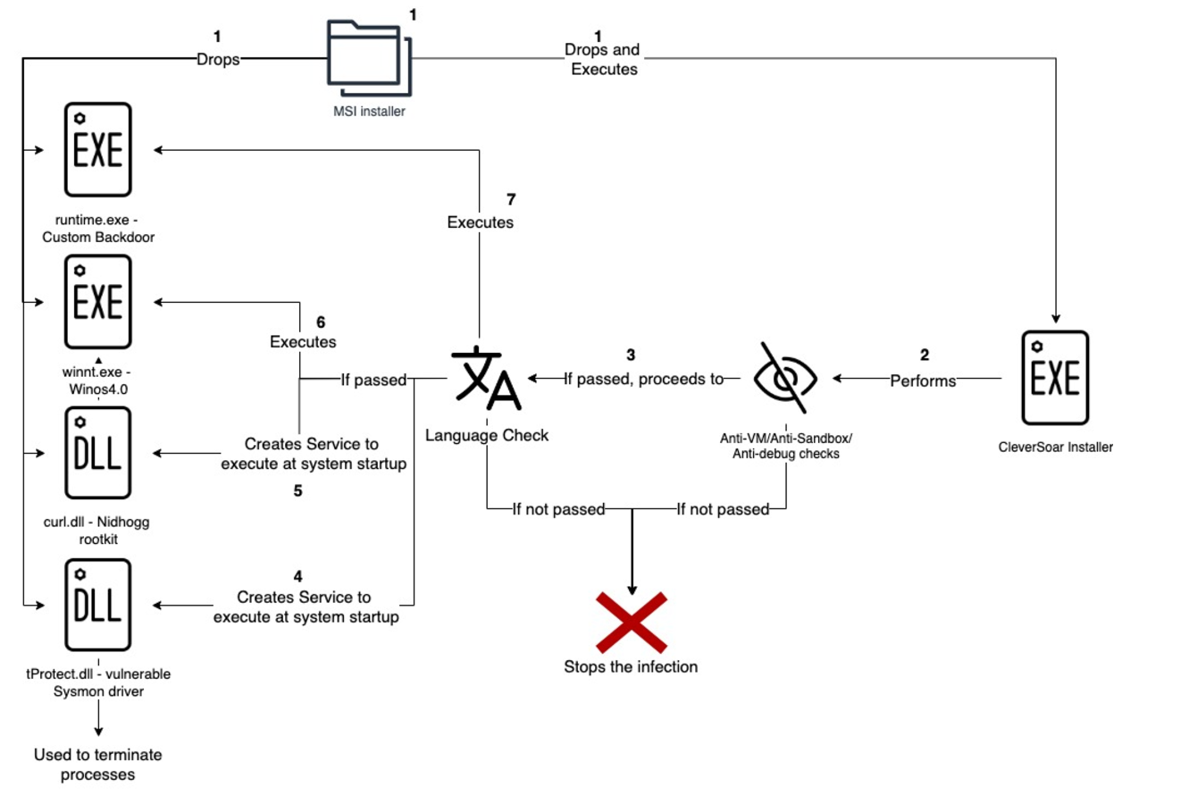
New “CleverSoar” Installer Targets Chinese and Vietnamese Users — Figure 1 – CleverSoar Attack Flow

File Information:

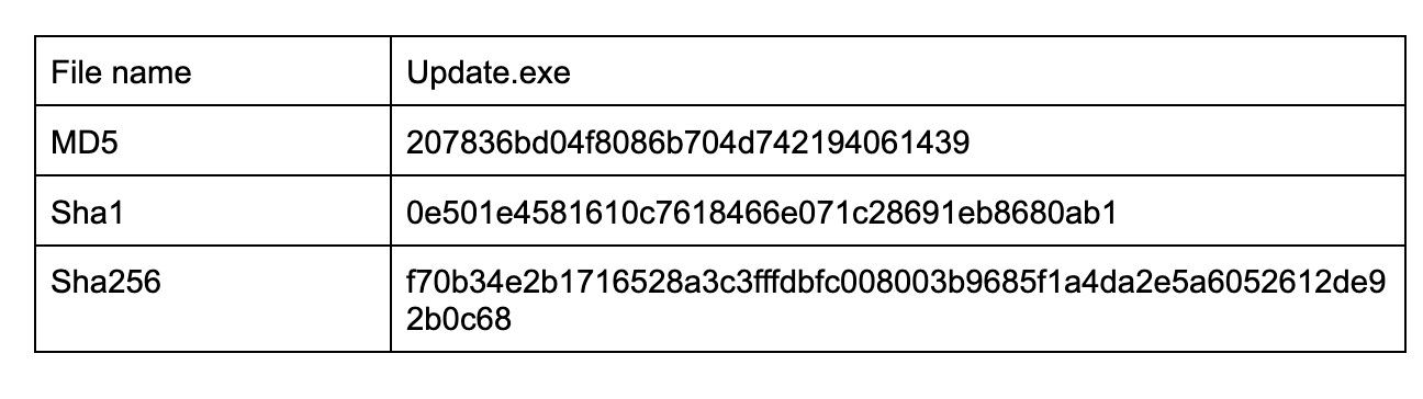
Given our high confidence that the malicious files were dropped by a .msi package (T1218.007), which in our case creates a ‘WindowsNT’ folder under the ‘C:\Program Files (x86)’ directory, we also assume that the same .msi package is responsible for dropping all the payloads listed below and executing the ‘Update.exe’ binary.

The installer begins by verifying the existence of the ‘C:\cs’ folder.It subsequently checks if the process is elevated by executing ‘GetTokenInformation’ and passing ‘TokenElevation’ (0x14) as a TokenInformationClass (T1134). If the process is not elevated, the malware will utilize the ‘runas’ operation of ‘ShellExecuteA’ to execute the process with Administrator privileges (T1134.002).

Subsequently, it proceeds to a series of evasion techniques, commencing with a rarely employed one.

Firmware Table Anti-VM

The malware retrieves a raw SMBIOS firmware table by invoking ‘GetSystemFirmwareTable’ and verifying a specific value presence. In our instance, the installer checks for ‘QEMU’ (indicating a free string open-sourced emulator) presence in the returned buffer (T1497.001). This technique is a sophisticated Anti-VM method as certain memory regions utilized by the operating system contain distinctive artifacts when the operating system is executed within a virtual environment. Notably, this technique has been previously employed by the Raspberry Robin malware, but in a slightly different way.

Windows Defender Emulator

The installer employs the ‘LdrGetDllHandleEx’ and ‘RtlImageDirectoryEntryToData’ functions to ascertain the state of Windows Defender’s emulator (T1497.001). Additionally, it utilizes the ‘NtIsProcessInJob’ and ‘NtCompressKey’ functions for the same purpose. These three anti-emulation techniques are publicly available in the UACME open-source project. Upon successful completion of these anti-emulation checks, the installer logs that defender checks were successfully bypassed and proceeds to the subsequent check.

Windows 10 or Windows 11

Initially, the installer verifies the operating system version by invoking the ‘GetVersionExW’ function (T1082). To identify whether the malware is executing on the Windows 10 operating system or Windows 11, the presence of the ‘C:\Windows\System32\Taskbar.dll’ file is checked, as this file can only be found on Windows 11 operating systems.

3rd Party DLL Injection Prevention

The CleverSoar installer modifies the processes mitigation policy to include the restriction ‘Signatures restricted (Microsoft only)’ (T1543). This action prevents non-Microsoft-signed binaries from being injected into the affected process. By implementing this technique, Anti-Virus and EDR solutions that employ userland hooking cannot inject their DLLs into the running process.

Timing Anti-Debug

The installer also executes timing anti-debug checks by invoking the ‘GetTickCount64’ function twice and measuring the delay between instructions and their execution (T1622).

Simple Anti-Debug check

The CleverSoar installer employs the ‘IsDebuggerPresent’ API call to ascertain whether the process is currently undergoing debugging (T1622).

Anti-Sandbox/Anti-VM Username Check

Upon the successful completion of all preceding checks, the malware retrieves the current username and subsequently compares it to the following (T1497.001):

‘CurrentUser, Sandbox, Emily, HAPUBWS, Hone Lee, IT-ADMIN, Johnaon, Miller, miloza, Peter Wilson, timmy, sand box, malware, maltest, test user, virus, John Doe, 9ZaXj, WALKER, vbccsb_*, vbccsb.’

While most of these usernames are well known for being used by sandboxes and emulator solutions, two of them seem to be misspelled: ‘Hone Lee’ instead of ‘Hong Lee’ and ‘Johnaon’ instead of ‘Johnson’.

There are two possible reasons for this misspell, first, the threat actor typed those names manually, and the second one might be, the threat actor found that those are more recent names used by sandboxes.

Once the username check bypass is successfully executed, the malware proceeds to complete the evasion phase and initiates its malicious actions.

Malicious Activity

Upon successful completion of all environmental checks, the installer proceeds to the system language verification. This process involves retrieving the language identifier (ID) for the user interface language and verifying if that ID corresponds to one of the Chinese language IDs (0x804, 0xC04, 0x1404, 0x1004) or the Vietnamese ID (0x42A). If the language ID does not match any of these identifiers, the malware terminates its execution (T1614.001).

This observation suggests a potential threat actor’s intention to target only endpoints within these two countries.

Subsequently, the installer creates the ‘HKCU\SOFTWARE\Magisk’ (T1112) registry key and searches for the ‘ring3_username’ value under it. If the value is not present, the malware retrieves the user name that the ‘explorer.exe’ process is running as and sets the ‘ring3_username’ value.

The installer verifies if virtualization is enabled in the firmware and made available by the operating system by calling ‘IsProcessorFeaturePresent’ with 0x15 (PF_VIRT_FIRMWARE_ENABLED) and creates the ‘INIT.dat’ file in the ‘C:\Program Files (x86)\Windows NT’ directory. Next, it enumerates processes and checks if one of ‘ZhuDongFangYu.exe’, ‘QHActiveDefense.exe’, ‘HipsTray.exe’, or ‘HipsDaemon.exe’ is running (T1518.001). The first two processes belong to 360 Total Security (Chinese Anti-Virus Software), and the last two belong to HeroBravo System Diagnostics. If one of these processes is discovered, the installer proceeds to adjust ‘Se_Debug_Privilege’ to the running process (T1134), enumerates running processes once again, searches for ‘lsass.exe’ and writes into that process (T1055). Unfortunately, we were unable to retrieve the written payload due to an unhandled runtime error. It is noteworthy that during our investigation, we identified several installer versions, and most of them encountered unhandled runtime errors and could not execute.

Upon successful completion of the preceding checks, the installer proceeds to verify the existence of the ‘CleverSoarInst’ service. If the service is not detected, the installer opens a named ‘\\.\pipe\ntsvcs’ pipe, which is linked to the RPC protocol, to establish a temporary service responsible for creating the ‘CleverSoar’ service (T1569.002). This temporary service will only execute once, executing the following command: ‘cmd /c start sc create CleverSoar’ displayname= CleverSoar binPath= “C:\Program Files (x86)\Windows NT\tProtect.dll” type= kernel start= auto’.

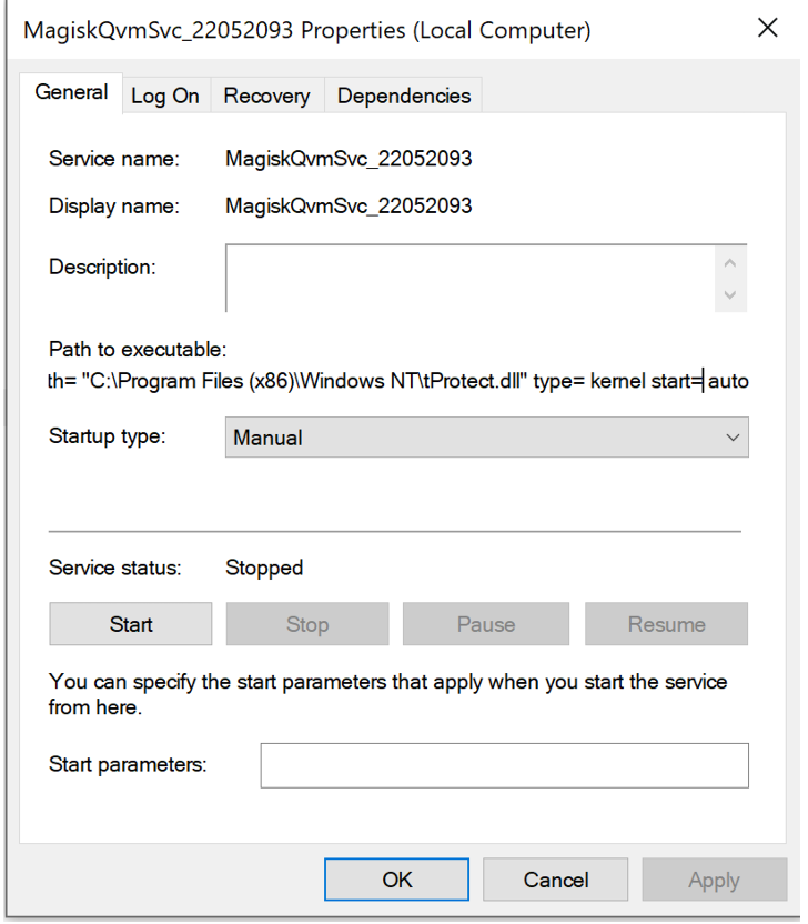
This command will create a new ‘CleverSoar’ service that will commence executing a driver at the system’s startup. The DLL specified within this service is one of the previously dropped files and is, in fact, a vulnerable Sysmon driver commonly employed by threat actors to disable security software. The installer initiates the ‘CleverSoar’ service and establishes a named ‘\\.\TfSysMon’ pipe connection. Subsequently, it enumerates the currently running processes once more (T1057), searching for any instances that contain one of the following strings:

Security Product	String
Bkav Pro	bka, blu
Windows Security	sechealthui, security, smartscreen, msmpeng, mssecess, mpcmdrun, defender
360 Total Security	360, zhudongfangyu, dsmain, qhactive, wdswfsafe, softmgr, 360se, 360chrome, 360zip
Kingsoft	ksafe, kwatch, kxecenter, kislive, kxetray, kxemain, kxewsc, kscan, kxescore, xdict
Huorong Internet Security	wsctrlsvc, usysdiag, hrsword
HeroBravo System Diagnostics	hips
Kaspersky	kav, avp, kis
2345 Security Guard	2345
Tencent	qqpc
McAfee	mcshield, mcapexe, mfemms
Avira	avira, sentryeye
Eset	eset, boothelper, efwd, egui, ekrn.exe, eguiproxy.exe
Elastic Security	elastic, agentbeat.exe, apm-server.exe
Rising Anti-Virus	ravmond.exe, rsmain.exe, rstray, rsmgrsvc
Monitoring and debugging tools	dbg, pchunter, hacker, monitor, wireshark
Other	lenovo, calc.exe, regedit
Unknown	remotectrlaid, superki, mfeavsv, 52pojie, kl_, watchdog

If one of the listed processes is discovered, the installer employs the ‘DeviceIoControl’ API call, specifying the process ID and the ‘0B4A00404h’ IoControl code. Upon our examination of the Sysmon driver, this action results in the termination of the identified process (T1489).

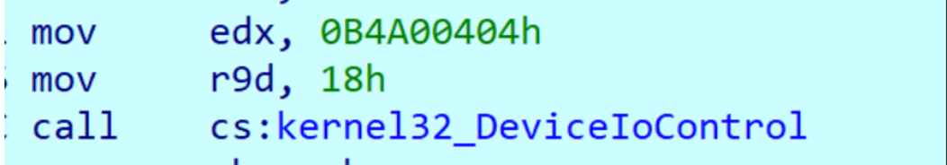
Subsequently, CleverSoar installer enumerates the files present in the folder generated by the malware and modifies their attributes by adding 0x6 (FILE_ATTRIBUTE_HIDDEN + FILE_ATTRIBUTE_SYSTEM). This modification is intended to evade file detection mechanisms (T1564.001).

The next phase involves the installation of a rootkit by creating a service which will run a rootkit dll in system startup. The installer initiates a verification process to ascertain the presence of a service named ‘Nidhogg.’ If the service is not already in existence, it proceeds to execute the command ‘sc create Nidhogg displayname= Nidhogg binPath= “C:\Program Files (x86)\Windows NT\curl.dll” type= kernel start= auto’ to create a new ‘Nidhogg’ service (T1543.003). The service will execute an open-sourced Nidhogg rootkit at system startup (T1014).

CleverSoar employs a persistence mechanism by executing a scheduled task upon user login (T1053). This task is initiated by dropping a .xml file into the user’s temporary folder, which contains a scheduled task XML file. By utilizing the same RPC service method previously mentioned, the installer constructs a service responsible for executing a command that creates the scheduled task with the ‘Corp’ name. The created task is concealed by modifying the ‘Index’ value under ‘HKEY_LOCAL_MACHINE\SOFTWARE\Microsoft\Windows NT\CurrentVersion\Schedule\TaskCache\Tree\Corp’ registry key to 0 (T1564).

After persistence set, the installer turns the Windows firewall off by executing the ‘netsh advfirewall set allprofiles state off’ command (T1562.004).

The malware now proceeds to the next stages of execution. Firstly, it checks if the ‘winnt.exe’ binary exists within the malware-created folder. In the event of its presence, the installer executes a command to create a scheduled task that will execute the binary once and immediately delete the scheduled task. The task responsible for executing the ‘winnt.exe’ is named ‘PayloadTask1’. If the binary is not present in the folder, the installer will persistently enumerate the folder and search for it. Based on our analysis of the ‘winnt.exe’ binary, it appears to be a Winos4.0 command-and-control (C2) framework implant that has recently been covered in Trend Micro’s report.

The installer executes the same process with the ‘runtime.exe’ binary. The task responsible for executing this binary is designated as ‘PayloadTask2’. Based on our investigation, ‘runtime.exe’ appears to be a custom backdoor, facilitating communication with the C2 server via a proprietary protocol.

By the time of the investigation the C2 server was already down and Rapid7 Labs could not continue the further analysis of interaction between the C2 server and the malware.

Conclusion

The CleverSoar campaign highlights an advanced and targeted threat, employing sophisticated evasion techniques and highly customized malware components like the Winos4.0 framework and Nidhogg rootkit. The campaign’s selective targeting of Chinese and Vietnamese-speaking users, along with its layered anti-detection measures, points to a persistent espionage effort by a capable threat actor. While currently aimed at individual users, this campaign’s tactics and tools demonstrate a level of sophistication that could easily extend to organizational targets. Organizations in the affected regions should take notice of the TTPs of this actor and monitor suspicious activity.

IOCs

F70b34e2b1716528a3c3fffdbfc008003b9685f1a4da2e5a6052612de92b0c68	CleverSoar installer
156.224.26.7	Winos4.0 C2
8848.twilight.zip	Backdoor C2

References

Nikon D700 Ten Minute Portrait Challenge – BUDGETOGRAPHY

2024-11-27 Matt Granger

Post Syndicated from Matt Granger original https://www.youtube.com/watch?v=WbYK35qgj-k