Post Syndicated from Giovanni Matteo Fumarola original https://aws.amazon.com/blogs/big-data/amazon-emr-streamlines-big-data-processing-with-simplified-amazon-s3-glacier-access/
Amazon S3 Glacier serves several important audit use cases, particularly for organizations that need to retain data for extended periods due to regulatory compliance, legal requirements, or internal policies. S3 Glacier is ideal for long-term data retention and archiving of audit logs, financial records, healthcare information, and other compliance-related data. Its low-cost storage model makes it economically feasible to store vast amounts of historical data for extended periods of time. The data immutability and encryption features of S3 Glacier uphold the integrity and security of stored audit trails, which is crucial for maintaining a reliable chain of evidence. The service supports configurable vault lock policies, allowing organizations to enforce retention rules and prevent unauthorized deletion or modification of audit data. The integration of S3 Glacier with AWS CloudTrail also provides an additional layer of auditing for all API calls made to S3 Glacier, helping organizations monitor and log access to their archived data. These features make S3 Glacier a robust solution for organizations needing to maintain comprehensive, tamper-evident audit trails for extended periods while managing costs effectively.
S3 Glacier offers significant cost savings for data archiving and long-term backup compared to standard Amazon Simple Storage Service (Amazon S3) storage. It provides multiple storage tiers with varying access times and costs, allowing optimization based on specific needs. By implementing S3 Lifecycle policies, you can automatically transition data from more expensive Amazon S3 tiers to cost-effective S3 Glacier storage classes. Its flexible retrieval options enable further cost optimization by choosing slower, less expensive retrieval for non-urgent data. Additionally, Amazon offers discounts for data stored in S3 Glacier over extended periods, making it particularly cost-effective for long-term archival storage. These features allow organizations to substantially reduce storage costs, especially for large volumes of infrequently accessed data, while meeting compliance and regulatory requirements. For more details, see Understanding S3 Glacier storage classes for long-term data storage.
Prior to Amazon EMR 7.2, EMR clusters couldn’t directly read from or write to the S3 Glacier storage classes. This limitation made it challenging to process data stored in S3 Glacier as part of EMR jobs without first transitioning the data to a more readily accessible Amazon S3 storage class.
The inability to directly access S3 Glacier data meant that workflows involving both active data in Amazon S3 and archived data in S3 Glacier were not seamless. Users often had to implement complex workarounds or multi-step processes to include S3 Glacier data in their EMR jobs. Without built-in S3 Glacier support, organizations couldn’t take full advantage of the cost savings in S3 Glacier for large-scale data analysis tasks on historical or infrequently accessed data.
Although S3 Lifecycle policies could move data to S3 Glacier, EMR jobs couldn’t easily incorporate this archived data into their processing without manual intervention or separate data retrieval steps.
The lack of seamless S3 Glacier integration made it challenging to implement a truly unified data lake architecture that could efficiently span across hot, warm, and cold data tiers.These limitations often required users to implement complex data management strategies or accept higher storage costs to keep data readily accessible for Amazon EMR processing. The improvements in Amazon EMR 7.2 aimed to address these issues, providing more flexibility and cost-effectiveness in big data processing across various storage tiers.
In this post, we demonstrate how to set up and use Amazon EMR on EC2 with S3 Glacier for cost-effective data processing.
Solution overview
With the release of Amazon EMR 7.2.0, significant improvements have been made in handling S3 Glacier objects:
- Improved S3A protocol support – You can now read restored S3 Glacier objects directly from Amazon S3 locations using the S3A protocol. This enhancement streamlines data access and processing workflows.
- Intelligent S3 Glacier file handling – Starting from Amazon EMR 7.2.0+, the S3A connector can differentiate between S3 Glacier and S3 Glacier Deep Archive objects. This capability prevents
AmazonS3Exceptionsfrom occurring when attempting to access S3 Glacier objects that have a restore operation in progress. - Selective read operations – The new version intelligently ignores archived S3 Glacier objects that are still in the process of being restored, enhancing operational efficiency.
- Customizable S3 Glacier object handling – A new setting,
fs.s3a.glacier.read.restored.objects, offers three options for managing S3 Glacier objects:- READ_ALL (Default) – Amazon EMR processes all objects regardless of their storage class.
- SKIP_ALL_GLACIER – Amazon EMR ignores S3 Glacier-tagged objects, similar to the default behavior of Amazon Athena.
- READ_RESTORED_GLACIER_OBJECTS – Amazon EMR checks the restoration status of S3 Glacier objects. Restored objects are processed like standard S3 objects, and unrestored ones are ignored. This behavior is the same as Athena if you configure the table property as described in Query restored Amazon S3 Glacier objects.
These enhancements provide you with greater flexibility and control over how Amazon EMR interacts with S3 Glacier storage, improving both performance and cost-effectiveness in data processing workflows.
Amazon EMR 7.2.0 and later versions offer improved integration with S3 Glacier storage, enabling cost-effective data analysis on archived data. In this post, we walk through the following steps to set up and test this integration:
- Create an S3 bucket. This will serve as the primary storage location for your data.
- Load and transition data:
- Upload your dataset to S3.
- Use lifecycle policies to transition the data to the S3 Glacier storage class.
- Create an EMR Cluster. Make sure you’re using Amazon EMR version 7.2.0 or higher.
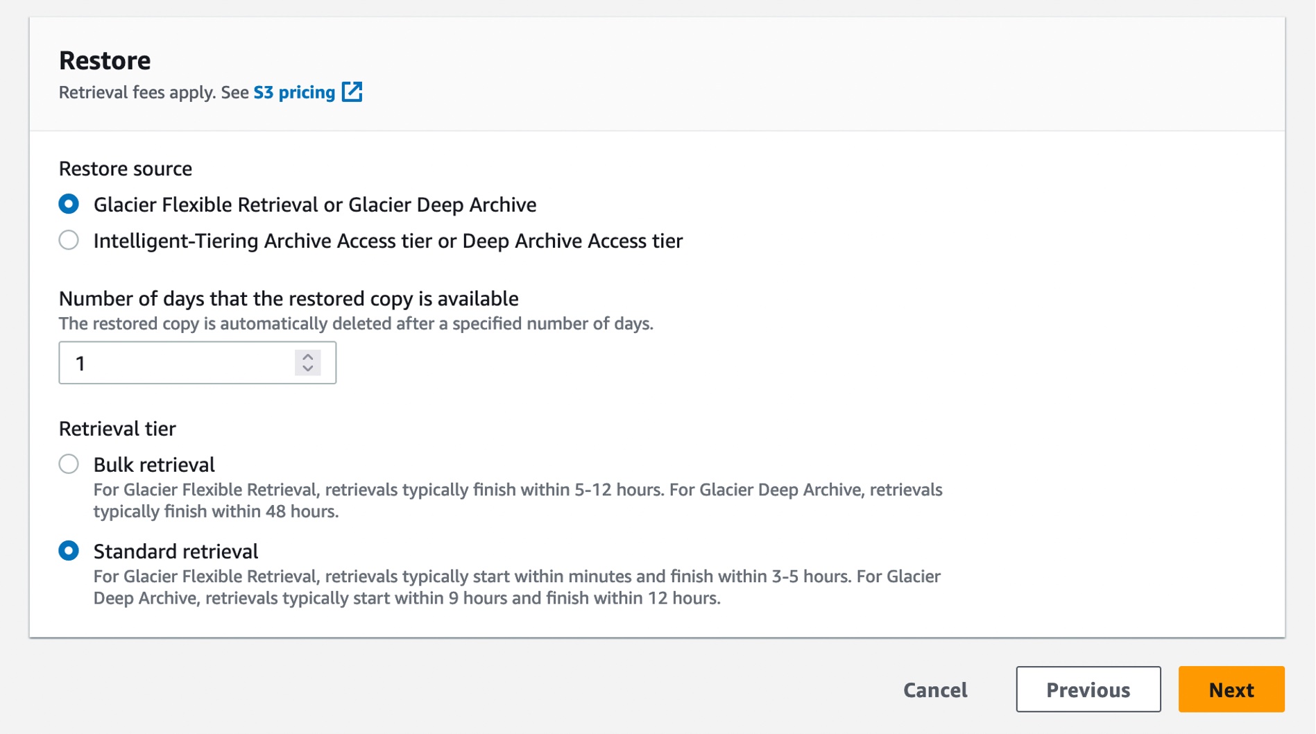
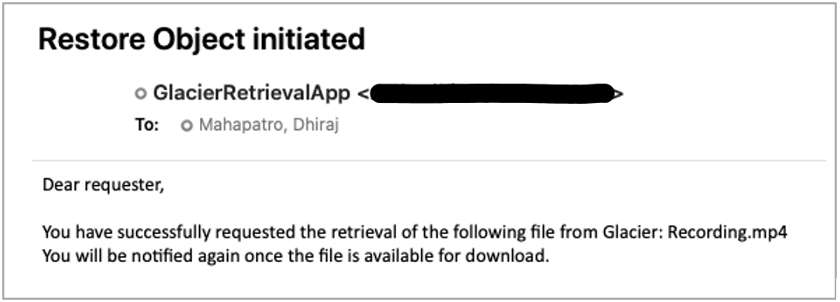
- Initiate data restoration by submitting a restore request for the S3 Glacier data before processing.
- To configure the Amazon EMR for S3 Glacier integration, set the
fs.s3a.glacier.read.restored.objectsproperty to READ_RESTORED_GLACIER_OBJECTS. This enables Amazon EMR to properly handle restored S3 Glacier objects. - Run Spark queries on the restored data through Amazon EMR.
Consider the following best practices:
- Plan workflows around S3 Glacier restore times
- Monitor costs associated with data restoration and processing
- Regularly review and optimize your data lifecycle policies
By implementing this integration, organizations can significantly reduce storage costs while maintaining the ability to analyze historical data when needed. This approach is particularly beneficial for large-scale data lakes and long-term data retention scenarios.
Prerequisites
The setup requires the following prerequisites:
- An active AWS account with appropriate permissions.
- An AWS Identity and Access Management (IAM) role with necessary permissions for Amazon EMR, Amazon S3, and S3 Glacier operations. For more information, see Configure IAM service roles for Amazon EMR permissions to AWS services and resources.
- Access to create and manage S3 buckets. For more information, refer to Creating a bucket.
- The ability to create and manage EMR clusters (version 7.2.0 or higher). For more information, see Tutorial: Getting started with Amazon EMR.
- An understanding of S3 Glacier storage classes and retrieval options. For more details, refer to the Amazon S3 Glacier Developer Guide.
- Knowledge for creating a cluster with Apache Spark. For more details, check here.
- A virtual private cloud (VPC) and subnet configurations for EMR cluster deployment. For more information, refer to Launch clusters into a VPC with Amazon EMR.
- An Amazon Elastic Compute Cloud (Amazon EC2) key pair for EMR cluster access. To learn more, see Amazon EC2 key pairs and Amazon EC2 instances.
- An allocated budget for AWS resource usage for running the example. For more details, see Managing your costs with AWS Budgets.
Create an S3 bucket
Create an S3 bucket with different S3 Glacier objects as listed in the following code:
For more information, refer to Creating a bucket and Setting an S3 Lifecycle configuration on a bucket.
The following is the list of objects:
The content of the objects is as follows:
S3 Glacier Instant Retrieval objects
For more information about S3 Glacier Instance Retrieval objects, see Appendix A at the end of this post. The objects are listed as follows:
The objects include the following contents:
To set different storage classes for objects in different folders, use the –storage-class parameter when uploading objects or change the storage class after upload:
S3 Glacier Flexible Retrieval objects
For more information about S3 Glacier Flexible Retrieval objects, see Appendix B at the end of this post. The objects are listed as follows:
The objects include the following contents:
To set different storage classes for objects in different folders, use the –storage-class parameter when uploading objects or change the storage class after upload:
S3 Glacier Deep Archive objects
For more information about S3 Glacier Deep Archive objects, see Appendix C at the end of this post. The objects are listed as follows:
The objects include the following contents:
To set different storage classes for objects in different folders, use the –storage-class parameter when uploading objects or change the storage class after upload:
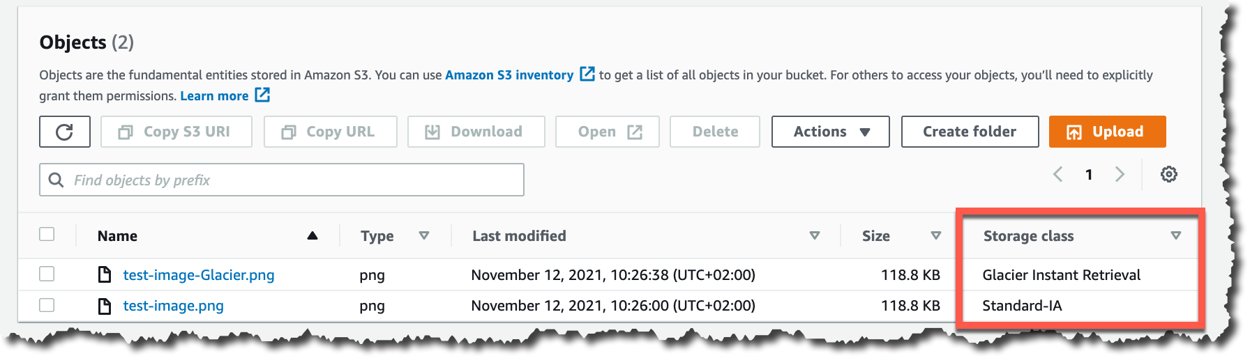
List the bucket contents
List the bucket contents with the following code:
Create an EMR Cluster
Complete the following steps to create an EMR Cluster:
- On the Amazon EMR console, choose Clusters in the navigation pane.
- Choose Create cluster.
- For the cluster type, choose Advanced configuration for more control over cluster settings.
- Configure the software options:
- Choose the Amazon EMR release version (make sure it’s 7.2.0 or higher for S3 Glacier integration).
- Choose applications (such as Spark or Hadoop).
- Configure the hardware options:
- Choose the instance types for primary, core, and task nodes.
- Choose the number of instances for each node type.
- Set the general cluster settings:
- Name your cluster.
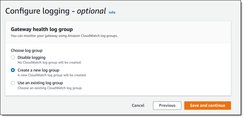
- Choose logging options (recommended to enable logging).
- Choose a service role for Amazon EMR.
- Configure the security options:
- Choose an EC2 key pair for SSH access.
- Set up an Amazon EMR role and EC2 instance profile.
- To configure networking, choose a VPC and subnet for your cluster.
- Optionally, you can add steps to run immediately when the cluster starts.
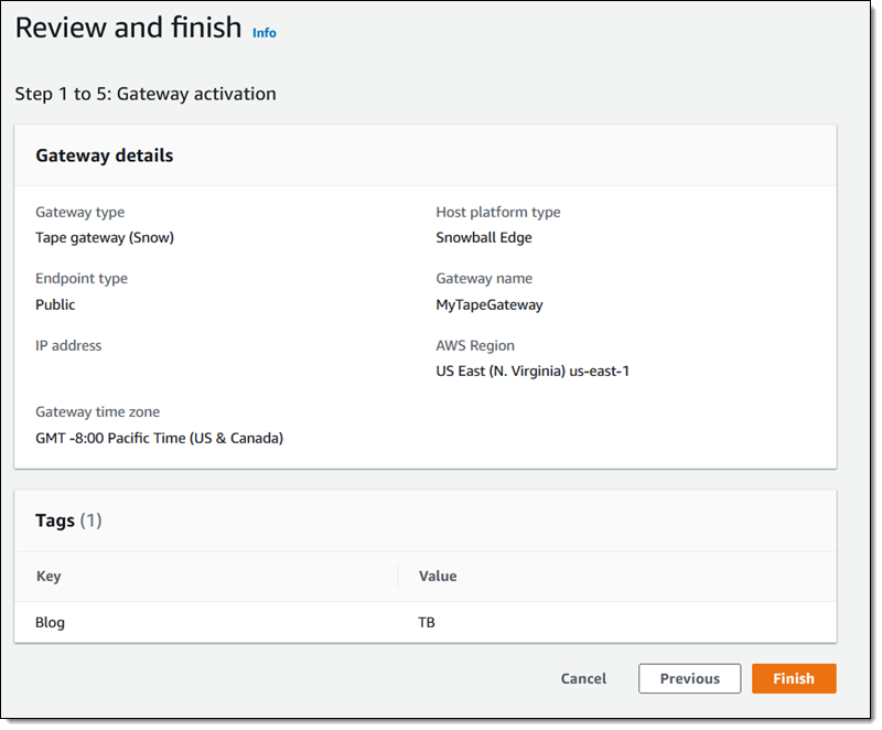
- Review your settings and choose Create cluster to launch your EMR Cluster.
For more information and detailed steps, see Tutorial: Getting started with Amazon EMR.
For additional resources, refer to Plan, configure and launch Amazon EMR clusters, Configure IAM service roles for Amazon EMR permissions to AWS services and resources, and Use security configurations to set up Amazon EMR cluster security.
Make sure that your EMR cluster has the necessary permissions to access Amazon S3 and S3 Glacier, and that it’s configured to work with the storage classes you plan to use in your demonstration.
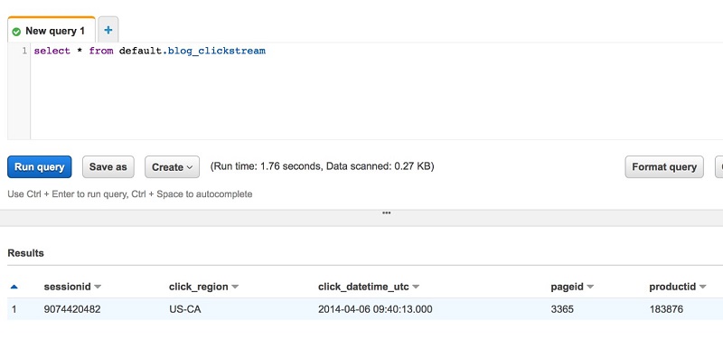
Perform queries
In this section, we provide code to perform different queries.
Create a table
Use the following code to create a table:
Queries before restoring S3 Glacier objects
Before you restore the S3 Glacier objects, run the following queries:
- ·READ_ALL – The following code shows the default behavior:
This option throws an exception reading the S3 Glacier storage class objects:
- SKIP_ALL_GLACIER – This option retrieves Amazon S3 Standard and S3 Glacier Instant Retrieval objects:
- READ_RESTORED_GLACIER_OBJECTS – The option retrieves standard Amazon S3 and all restored S3 Glacier objects. The S3 Glacier objects are under retrieval and will show up after they are retrieved.
Queries after restoring S3 Glacier objects
Perform the following queries after restoring S3 Glacier objects:
- READ_ALL – Because all the objects have been restored, all the objects are read (no exception is thrown):
- SKIP_ALL_GLACIER – This option retrieves standard Amazon S3 and S3 Glacier Instant Retrieval objects:
- READ_RESTORED_GLACIER_OBJECTS – The option retrieves standard Amazon S3 and all restored S3 Glacier objects. The S3 Glacier objects are under retrieval and will show up after they are retrieved.
Conclusion
The integration of Amazon EMR with S3 Glacier storage marks a significant advancement in big data analytics and cost-effective data management. By bridging the gap between high-performance computing and long-term, low-cost storage, this integration opens up new possibilities for organizations dealing with vast amounts of historical data.
Key benefits of this solution include:
- Cost optimization – You can take advantage of the economical storage options of S3 Glacier while maintaining the ability to perform analytics when needed
- Data lifecycle management – You can benefit from a seamless transition of data from active S3 buckets to archival S3 Glacier storage, and back when analysis is required
- Performance and flexibility – Amazon EMR is able to work directly with restored S3 Glacier objects, providing efficient processing of historical data without compromising on performance
- Compliance and auditing – The integration offers enhanced capabilities for long-term data retention and analysis, which are crucial for industries with strict regulatory requirements
- Scalability – The solution scales effortlessly, accommodating growing data volumes without significant cost increases
As data continues to grow exponentially, the Amazon EMR and S3 Glacier integration provides a powerful toolset for organizations to balance performance, cost, and compliance. It enables data-driven decision-making on historical data without the overhead of maintaining it in high-cost, readily accessible storage.
By following the steps outlined in this post, data engineers and analysts can unlock the full potential of their archived data, turning cold storage into a valuable asset for business intelligence and long-term analytics strategies.
As we move forward in the era of big data, solutions like this Amazon EMR and S3 Glacier integration will play a crucial role in shaping how organizations manage, store, and derive value from their ever-growing data assets.
About the Authors
 Giovanni Matteo Fumarola is the Senior Manager for EMR Spark and Iceberg group. He is an Apache Hadoop Committer and PMC member. He has been focusing in the big data analytics space since 2013.
 Narayanan Venkateswaran is an Engineer in the AWS EMR group. He works on developing Hive in EMR. He has over 17 years of work experience in the industry across several companies including Sun Microsystems, Microsoft, Amazon and Oracle. Narayanan also holds a PhD in databases with focus on horizontal scalability in relational stores.
 Karthik Prabhakar is a Senior Analytics Architect for Amazon EMR at AWS. He is an experienced analytics engineer working with AWS customers to provide best practices and technical advice in order to assist their success in their data journey.
Appendix A: S3 Glacier Instant Retrieval
S3 Glacier Instant Retrieval objects store long-lived archive data accessed once a quarter with instant retrieval in milliseconds. These are not distinguished from S3 Standard object, and there is no option to restore them as well. The key difference between S3 Glacier Instant Retrieval and standard S3 object storage lies in their intended use cases, access speeds, and costs:
- Intended use cases – Their intended use cases differ as follows:
- S3 Glacier Instant Retrieval – Designed for infrequently accessed, long-lived data where access needs to be almost instantaneous, but lower storage costs are a priority. It’s ideal for backups or archival data that might need to be retrieved occasionally.
- Standard S3 – Designed for frequently accessed, general-purpose data that requires quick access. It’s suited for primary, active data where retrieval speed is essential.
- Access speed – The differences in access speed are as follows:
- S3 Glacier Instant Retrieval – Provides millisecond access similar to standard Amazon S3, though it’s optimized for infrequent access, balancing quick retrieval with lower storage costs.
- Standard S3 – Also offers millisecond access but without the same access frequency limitations, supporting workloads where frequent retrieval is expected.
- Cost structure – The cost structure is as follows:
- S3 Glacier Instant Retrieval – Lower storage cost compared to standard Amazon S3 but slightly higher retrieval costs. It’s cost-effective for data accessed less frequently.
- Standard S3 – Higher storage cost but lower retrieval cost, making it suitable for data that needs to be frequently accessed.
- Durability and availability – Both S3 Glacier Instant Retrieval and standard Amazon S3 maintain the same high durability (99.999999999%) but have different availability SLAs. Standard Amazon S3 generally has a slightly higher availability, whereas S3 Glacier Instant Retrieval is optimized for infrequent access and has a slightly lower availability SLA.
Appendix B: S3 Glacier Flexible Retrieval
S3 Glacier Flexible Retrieval (previously known simply as S3 Glacier) is an Amazon S3 storage class for archival data that is rarely accessed but still needs to be preserved long-term for potential future retrieval at a very low cost. It’s optimized for scenarios where occasional access to data is required but immediate access is not critical. The key differences between S3 Glacier Flexible Retrieval and standard Amazon S3 storage are as follows:
- Intended use cases – Best for long-term data storage where data is accessed very infrequently, such as compliance archives, media assets, scientific data, and historical records.
- Access options and retrieval speeds – The differences in access and retrieval speed are as follows:
- Expedited – Retrieval in 1–5 minutes for urgent access (higher retrieval costs).
- Standard – Retrieval in 3–5 hours (default and cost-effective option).
- Bulk – Retrieval within 5–12 hours (lowest retrieval cost, suited for batch processing).
- Cost structure – The cost structure is as follows:
- Storage cost – Very low compared to other Amazon S3 storage classes, making it suitable for data that doesn’t require frequent access.
- Retrieval cost – Retrieval incurs additional fees, which vary depending on the speed of access required (Expedited, Standard, Bulk).
- Data retrieval pricing – The quicker the retrieval option, the higher the cost per GB.
- Durability and availability – Like other Amazon S3 storage classes, S3 Glacier Flexible Retrieval has high durability (99.999999999%). However, it has lower availability SLAs compared to standard Amazon S3 classes due to its archive-focused design.
- Lifecycle policies – You can set lifecycle policies to automatically transition objects from other Amazon S3 classes (like S3 Standard or S3 Standard-IA) to S3 Glacier Flexible Retrieval after a certain period of inactivity.
Appendix C: S3 Glacier Deep Archive
S3 Glacier Deep Archive is the lowest-cost storage class of Amazon S3, designed for data that is rarely accessed and intended for long-term retention. It’s the most cost-effective option within Amazon S3 for data that can tolerate longer retrieval times, making it ideal for deep archival storage. It’s a perfect solution for organizations with data that must be retained but not frequently accessed, such as regulatory compliance data, historical archives, and large datasets stored purely for backup. The key differences between S3 Glacier Deep Archive and standard Amazon S3 storage are as follows:
- Intended use cases – S3 Glacier Deep Archive is ideal for data that is infrequently accessed and requires long-term retention, such as backups, compliance records, historical data, and archive data for industries with strict data retention regulations (such as finance and healthcare).
- Access options and retrieval speeds – The differences in access and retrieval speed are as follows:
- Standard retrieval – Data is typically available within 12 hours, intended for cases where occasional access is required.
- Bulk retrieval – Provides data access within 48 hours, designed for very large datasets and batch retrieval scenarios with the lowest retrieval cost.
- Cost structure – The cost structure is as follows:
- Storage cost – S3 Glacier Deep Archive has the lowest storage costs across all Amazon S3 storage classes, making it the most economical choice for long-term, infrequently accessed data.
- Retrieval cost – Retrieval costs are higher than more active storage classes and vary based on retrieval speed (Standard or Bulk).
- Minimum storage duration – Data stored in S3 Glacier Deep Archive is subject to a minimum storage duration of 180 days, which helps maintain low costs for truly archival data.
- Durability and availability – It offers the following durability and availability benefits:
- Durability – S3 Glacier Deep Archive has 99.999999999% durability, similar to other Amazon S3 storage classes.
- Availability – This storage class is optimized for data that doesn’t need frequent access, and so has lower availability SLAs compared to active storage classes like S3 Standard.
- Lifecycle policies – Amazon S3 allows you to set up lifecycle policies to transition objects from other storage classes (such as S3 Standard or S3 Glacier Flexible Retrieval) to S3 Glacier Deep Archive based on the age or access frequency of the data.


 Lastly, we published a new ebook titled “


 Ten years ago, on August 20, 2012, AWS


 We launched
 This team came together to build a best-in-class gene-editing prediction platform. CRISPR (


 Thiyagarajan Arumugam is a Principal Solutions Architect at Amazon Web Services and designs customer architectures to process data at scale. Prior to AWS, he built data warehouse solutions at Amazon.com. In his free time, he enjoys all outdoor sports and practices the Indian classical drum mridangam.
 Srinivasan Krishnasamy is a ‘Senior Big Data Consultant’ at Amazon Web Services. He joined AWS in 2015 and specializes in building and supporting Big Data solutions that help customers to ingest, process and analyze data at scale.
 Satish Sathiya is a Product Engineer at Amazon Redshift. He is an avid big data enthusiast who collaborates with customers around the globe to achieve success and meet their data warehousing and data lake architecture needs.


 David Roberts is a Senior Solutions Architect at AWS. His passion is building efficient and effective solutions on the cloud, especially involving analytics and data lake governance. Besides spending time with his wife and two daughters, he likes drumming and watching movies, and is an avid video gamer.