Netflix Stratum Media Processing: Automated Container Right-Sizing

Post Syndicated from Netflix Technology Blog original https://netflixtechblog.com/netflix-stratum-media-processing-automated-container-right-sizing-ddf9aa68a801

By Violetta Pidvolotska and Naveen Mareddy

Stratum is Netflix’s internal serverless media processing platform, shaped by over a decade of experience developing large-scale distributed systems. It powers a wide range of media workloads — including encoding, packaging, inspection, and quality scoring — behind playback, advertising, studio workflows, AI embeddings, and more.

Engineers develop Stratum functions by packaging application code and OS dependencies into OCI images. Stratum then schedules these containers as batch jobs on Netflix’s Titus compute platform, with upstream services triggering function executions.

Every day, Stratum manages hundreds of thousands of containers across bursty, high-throughput, and latency-sensitive workloads. As Netflix’s core media processing platform, this load needs to scale as new content formats enter the catalog, such as podcasts, live events, sports, ads, or regional ingests like TF1 in France.

To request resources for these functions, owners specify their CPU, memory, disk, and network limits as YAML configuration, as shown below:

functionName: VideoEncoder.encodeV1
resources:
numCpus: 8
memoryInMB: 18000
diskSizeInMB: 50000
networkInMbps: 1000

Maintaining optimal values manually is challenging amidst evolving Netflix infrastructure, EC2 instance upgrades, and application-level changes. Consequently, configs are often over-provisioned upfront or slowly drift away from their ideal values over time. Mis-sized configurations are a universal pain of large-scale serverless platforms, causing additional cognitive load for function builders and operational costs for platform owners.

In this post, we share how we built the Stratum Resource Tuner (SRT) — an automated system that safely right-sizes running containers in production without human intervention. We will walk through real-world examples, our safety architecture, and what we learned when an automated change went wrong.

The Challenge: Over-Provisioning

When engineers write a new Stratum function, they typically copy a resource YAML from an existing function or size it for the absolute worst-case scenario. Once running in production, engineers rarely revisit these configurations until a failure occurs, prompting them to over-provision resources out of an abundance of caution.

Manual resource tuning does not scale for the following reasons:

  • High Operational Friction: Downsizing requires days of manual metric monitoring and trial-and-error testing, diverting valuable engineering cycles away from other high-impact work. If a cut goes too far, engineers face production incidents — making manual tuning a high-risk, low-reward task.
  • Continuous Infrastructure & Codec Evolution: Cloud providers regularly upgrade their hardware. A resource allocation that was optimal on an older hardware generation quietly becomes inefficient on newer hardware. At the same time, Netflix continuously advances media standards and improves encoding algorithms (such as AV1, AV2, and spatial audio). An allocation tuned for one codec might not be optimal when an improved algorithm is released.
  • Dynamic Workload Evolution: As Netflix expands into new media types — such as streaming video podcasts, sports, interactive AI-adapted ad formats, and major broadcaster integrations like TF1 in France — media processing footprints can change unpredictably, rendering static container resource limits imprecise.
  • Rising Industry Hardware Costs: Driven by massive global AI infrastructure demand, server hardware and DRAM prices continue to climb, making idle container memory significantly more expensive to waste.
  • Compounding Platform Scale: At Netflix scale, even minor over-provisioning multiplies exponentially across hundreds of thousands of daily container executions, compounding wasted capacity across the entire Stratum platform.

To understand the scale of the challenge, we analyzed historical usage across Stratum’s workloads. The telemetry confirmed our hypothesis: over-provisioning was frequent, wasted compute was compounding, and the sustainable path forward required a fundamental re-evaluation of how resource configurations are managed.

Meet the Stratum Resource Tuner

To address the challenges listed above, we built the Stratum Resource Tuner (SRT) to automatically right-size Stratum containers. Our north star is to ensure that users never have to manually specify the resource configurations. We started with a handful of high-throughput workloads with relaxed latency requirements, which account for the majority (70%–80%) of resource usage.

As a quick note on terminology, we use “right-sizing” and “tuning” interchangeably in this post. “Downsizing” means decreasing resource limits, while “upsizing” means increasing them. Since our goal is to optimize for cost, this post focuses on downsizing.

Automatic right-sizing is not enabled by default. Function owners must manually opt in on a per resource type basis (e.g., CPU, memory, network, or disk). Once enrolled, SRT operates without a human in the loop across five steps:

Figure 1: SRT Workflow High-Level
  1. Collect resource usage metrics across all executions of that function.
  2. Generate a recommendation for each resource type (e.g., CPU or memory).
  3. Verify the recommendation through experiments.
  4. Apply or reject the recommendation based on the results of experiments.
  5. Monitor post-apply metrics, watching for anomalies after applying the recommendation.

“Recommendation” is a key construct in SRT and serves as the primary unit of operation. As SRT executes its steps, it promotes the recommendation through several stages:

Figure 2: Recommendation State Machine
  • CREATED: A scheduled workflow generated the recommendation.
  • EVALUATING: Recommendation verification is running, and SRT is analyzing the results.
  • APPLIED: All experiments passed, and SRT automatically rolled out the recommended configuration.
  • REJECTED: At least one experiment failed, leaving the function configuration untouched.
  • MONITORED: SRT monitors the recommendation during a post-apply soak period to verify stability.

The sections below examine each of these stages in detail. To illustrate the flow, we will follow the real-world lifecycle of the VideoEncoder.encodeV1 function — a high-throughput video encoding function whose over-provisioned memory and CPU footprints were successfully tuned.

Note that all operational thresholds and safety limits discussed below are fully configurable per function to accommodate varying workload characteristics and risk tolerances.

Metrics Collection

To make these recommendations possible, we need a solid metrics collection mechanism. Every Stratum container reports its function execution metadata, infrastructure dimensions, and resource utilization (CPU, memory, disk, and network) at sub-minute resolution.

These metrics flow through Keystone, Netflix’s real-time event streaming platform, and land in two separate datastores:

Figure 3: Metrics Collection
  • Execution summaries store: Stores execution-level summary metrics indexed in Elasticsearch for fast point lookups, serving as our short-term datastore for querying and inspecting individual runs.
  • High-resolution long-term store: Stores raw, high-resolution usage metrics in Iceberg tables. While slower to query, it serves as our long-term datastore, holding months of history for resource utilization trend analysis.

One record is written per execution, which is represented as a span. Here is how these records look for a single span of our VideoEncoder.encodeV1 function.

In Elasticsearch, the record captures the high-level summary of the completed span, identified by tags.stratum.spanId:

{
"tags.stratum.spanId": "38536313f65f060a",
"tags.functionName": "VideoEncoder.encodeV1",
"tags.stratum.phase": "run",
"tags.stratum.success": true,
"tags.stratum.retriedWithMoreResources": false,
"tags.stratum.function.execDurationSecs": 26,
"tags.cpuCount": 8,
"tags.memoryInMB": 18000,
"tags.diskInMB": 50000,
"tags.networkInMbps": 1000,
"tags.titusTaskId": "06e1a7c0-2502-4a54-905f-b13a1e786107",
"tags.instanceType": "r7a.24xlarge",
"tags.nf.region": "us-east-1",
"ts": 1780743028000
}

In Iceberg, the record contains the same metadata, but adds the sub-minute resource utilization timeseries tracked during that span:

{
"span_id": "38536313f65f060a",
"function_name": "VideoEncoder.encodeV1",
"phase": "run",
"success": true,
"start_epoch_secs": 1780743002,
"end_epoch_secs": 1780743028,
"runtime_secs": 26,
"cpu_requested": 8,
"memory_mb_requested": 18000,
"disk_mb_requested": 50000,
"network_mbps_requested": 1000,
"titusTaskId": "06e1a7c0-2502-4a54-905f-b13a1e786107",
"instance_type": "r7a.24xlarge",
"tags.stratum.retriedWithMoreResources": false,
"env": "prod",
"resource_usage": [
{ "cpu_usage": 1.13, "memory_mb": 3701.37, "disk_mb": 20120.4, "net_in_mb": 221.09, "net_out_mb": 0.12 },
{ "cpu_usage": 2.25, "memory_mb": 3584.09, "disk_mb": 25410.1, "net_in_mb": 0.02, "net_out_mb": 0.05 },
{ "cpu_usage": 4.16, "memory_mb": 6750.79, "disk_mb": 30400.5, "net_in_mb": 165.90, "net_out_mb": 0.38 },
...
]
}

Recommendation Generation

A scheduled Conductor workflow runs daily, reading the past month of usage data from Iceberg and generating recommendations for every function and resource type. The workflow also generates recommendations for functions that have not opted into automatic right-sizing to preview potential savings.

Each recommendation is saved in the recommendations datastore, enabling us to query and filter recommendations by function, resource type, or status on an ad hoc basis.

Figure 4: Recommendation Generation Sequence

For each function and resource type, the workflow applies the following generation logic:

  • Filter by workload type: We only tune high-throughput workloads. This focuses our efforts on right-sizing, which yields the most meaningful fleet-wide savings.
  • Aggressively tune CPU and network: We target p99 usage with no extra headroom. CPU and network are compressible resources; if a container occasionally hits these limits, the function might execute slightly slower.
  • Conservatively tune memory and disk: We target p99.9 usage and include a safety buffer. Running out of physical memory or disk space causes hard failures — such as Out of Memory (OOM) or Out of Disk (OOD) crashes — making a protective margin essential.
  • Apply safeguards to changes: We discard recommendations if the absolute reduction is too small to justify operational effort. For memory and disk, we clamp the maximum reduction allowed in a single cycle to 15% — a safety limit introduced after learning from early production runs.

The workflow creates new recommendations in the CREATED state. If a recommendation already exists in this state for a given function and resource type, SRT overwrites it with updated calculations. Once a recommendation advances past the CREATED state, its recommended_value and stats fields become immutable. Subsequent daily runs generate a new recommendation with a unique ID instead of modifying the existing record.

Here is how these recommendations look across resource types in their initial CREATED state for our VideoEncoder.encodeV1 function:

  • CPU recommendation
{

"function_name": "VideoEncoder.encodeV1",
"env": "prod", "resource_type": "CPU",
"current_value": 8, "recommended_value": 4,
"status": "CREATED",
"resource_cost_usd_per_hour": ***,
"stats": {
"usage": { "p99": 4.16, "p999": 4.57 },
"execution": {
"total_fn_executions": 748762182,
"success_fn_executions_pct": 99.75,
"total_fn_exec_runtime_hr": 88102723
},
"window": { "start": "2026-05-05T00:00:00Z", "end": "2026-06-05T00:00:00Z" }
},
"experiment_inputs": null,
"experiment_workflow_execution_id": null,
"outcome_message": null,
"finalized_at": null
}
  • Memory recommendation (15% reduction in one step)
{
"id": "2edb734a-6184-4f5e-8ffa-23004bd665d7",
"function_name": "VideoEncoder.encodeV1",
"env": "prod", "resource_type": "MEMORY_MB",
"current_value": 18000, "recommended_value": 15300,
"status": "CREATED",
"resource_cost_usd_per_hour": ***,

"stats": {
"usage": { "avg": 5296.43, "p99": 6750.8, "p999": 7820.3 },
"execution": {
"total_fn_executions": 748762182,
"success_fn_executions_pct": 99.75,
"total_fn_exec_runtime_hr": 88102723
},
"window": { "start": "2026-05-05T00:00:00Z", "end": "2026-06-05T00:00:00Z" }
},
"experiment_inputs": null,
"experiment_workflow_execution_id": null,
"outcome_message": null,
"finalized_at": null
}

As the recommendation moves through its lifecycle, SRT populates the remaining parameters.

When proceeding to the verification stage, SRT transitions the recommendation status to EVALUATING, records the target experiment settings, and links the active workflow execution tracking the experiment.

Finally, once verification runs complete, the status changes to APPLIED or REJECTED, storing the outcome details and completion timestamp for analysis.

Retry with More Resources

We take a conservative approach to generating recommendations, prioritizing system stability over extreme efficiency. Because recommendations rely on historical usage data, they cannot always anticipate sudden spikes or novel workload profiles when functions encounter heavy, unseen requests.

To handle these unexpected spikes, we developed a fail-safe mechanism. A watcher process running in each tuned container tracks memory and disk usage during function execution. If the container exceeds the pre-set thresholds, 85% for non-cached memory usage or 95% for disk usage, the watcher flags the execution as high risk, cancels execution, and re-queues the task onto a larger container:

new_container_size = original_container_size * 1.5

This 1.5 multiplier only applies to memory and disk dimensions.

Figure 5: Retry with More Resources

This “retry with more resources” mechanism serves as our safety net: larger container configurations are applied only when retrying tasks to self-heal from edge cases. Although these infrequent retries incur additional compute costs and latency, they allow us to keep day-to-day configurations highly optimized without having to size for rare, costly outliers up front.

For our VideoEncoder.encodeV1 function, if a heavy run causes memory usage to exceed the 85% threshold (15,300 MB) within its current 18,000 MB container, the system aborts the execution and reruns it on a 27,000 MB container.

While we prefer to trigger retries based on actual OOM or OOD events rather than pre-set thresholds, technical constraints in our current architecture make true event detection challenging. Using pre-set thresholds serves as a reliable stopgap while we develop improved detection capabilities.

SRT automatically enables the retry mechanism for any function opted into memory or disk right-sizing. Each Stratum container reports retry events, which flow into Elasticsearch and Iceberg alongside standard performance telemetry.

Recommendation Verification

Every recommendation must pass a two-stage verification process managed by a Conductor workflow before rollout. During this EVALUATING stage, SRT executes two distinct experiment types:

  1. Synthetic experiment: A low-cost, low-risk test to catch obvious regressions before production rollout.
  2. Production experiment: A live evaluation that validates changes across diverse production workloads to increase confidence.

A recommendation advances to production testing only after passing the synthetic experiment. When an opted-in function has multiple pending recommendations, SRT prioritizes and evaluates the candidates with the highest estimated savings first.

Figure 6: Evaluating Stage

Synthetic experiment:

  • Runs in a test environment isolated from production traffic.
  • Sets up two clusters: one for the current and one for the recommended config.
  • Replays identical request sets across both clusters simultaneously without splitting traffic, exposing both configurations to 100% of test requests.
  • Typically runs for 1–2 hours.
  • Runs to completion without early termination checks.
Figure 7: Synthetic Experiment Flow

Production experiment:

  • Runs in production on real user traffic, split three ways:
    ◦ ~90% remains on the main cluster (current production config).
    ◦ ~5% goes to a baseline cluster (current production config).
    ◦ ~5% goes to an experimental cluster (recommendation config).
  • Evaluates recommendations against a similarly sized baseline cluster rather than the main cluster to preserve comparable traffic profiles.
  • Typically runs from one day to one week, depending on traffic volume.
  • Fails fast: cancels the experiment early if regressions are detected.
Figure 8: Production Experiment Flow

The Stratum platform executes other experiments alongside SRT experiments. To avoid over-splitting traffic, SRT experiments run at lower priority and yield resources to active, higher-priority experiments.

Traffic arrives in irregular bursts separated by multi-day or multi-week lulls. The verification pipeline accommodates these variable arrival patterns rather than expecting steady traffic.

Back to our VideoEncoder.encodeV1 memory recommendation (18,000 MB → 15,300 MB), verification is triggered with:

{
"recommendationId": "2edb734a-6184-4f5e-8ffa-23004bd665d7",
"syntheticExperiment": { "numberOfExecutions": 3000 },
"productionExperiment": {
"enabled": true,
"maxContainers": 20, // max containers shift to baseline & experimental clusters
"upGateTimeoutMinutes": 10080, // time to wait for traffic to start flowing
"maxRunDurationMinutes": 1240, // max time to run the experiment once traffic starts
"minSamples": 500 // min executions needed on both clusters before evaluating
}
}

Both verification stages evaluate recommendations against two sequential checks, terminating immediately if either fails:

  • Retries with more resources: Restricts memory and disk downsizes to a maximum 1% retry threshold over the experiment duration.
  • Execution time: Compares median runtimes to prevent outlier distortion, permitting up to a 10–15% slowdown relative to baseline, depending on workload, and is configurable by function.

If a recommendation passes both verification stages, SRT updates its status to APPLIED and rolls out the configuration to the main production cluster. If a check fails at any point, SRT marks the recommendation as REJECTED and preserves the existing configuration. SRT sends notifications for both outcomes.

For VideoEncoder.encodeV1, both stages passed cleanly:

{
"outcome": "APPLIED",
"syntheticExperiment": {
"result": "SUCCESS",
"samples": { "baseline": 3000, "experimental": 3000 },
"medianExecutionSecs": { "baseline": 59.0, "experimental": 59.0 },
"slownessIncreasePct": 0.0,
"retryRatePct": { "baseline": 0.0, "experimental": 0.0 }
},
"productionExperiment": {
"result": "SUCCESS",
"samples": { "baseline": 50361, "experimental": 49790 },
"medianExecutionSecs": { "baseline": 196.0, "experimental": 198.0 },
"slownessIncreasePct": 1.0,
"retryRatePct": { "baseline": 0.0, "experimental": 0.0 }
}
}

The recommendation moved to the APPLIED state, permanently setting the memory allocation for VideoEncoder.encodeV1 to 15,300 MB. We observed similarly clean results for the CPU recommendation, which reduced CPU allocation from 8 cores to 4.

Post-Apply Monitoring

Passing verification experiments does not mark the end of the recommendation lifecycle. Updated function code, modified input parameters, or underlying changes in the compute environment (Titus/EC2) can alter production behavior over time. To ensure configuration safety and foster feature adoption, we instituted continuous post-apply monitoring for applied changes.

We monitor metrics for 90 days across two rolling time windows: a 30-minute fast window and a 24-hour slow window. Each window maintains specific alert thresholds: a 3% retry rate over 30 minutes or a 2% rate over 24 hours triggers an automated notification.

At steady state, workloads exhibit baseline retry rates around 0.1%, with rates up to 2%–3% falling within acceptable operational variances. Most applied recommendations remained stable over the past three months.

VideoEncoder.encodeV1 has operated on its tuned configuration for months without breaching thresholds. However, VideoEncoder.encodeV2 presented a challenging edge case: a 50% memory reduction passed all verification checks and ran stably for two weeks before an unexpected traffic shift drove retry rates above 60%.

Figure 9: Unexpected Retries Spike

Because early versions lacked automated rollback capabilities, engineers manually triaged exception cases. This incident highlighted the need for automated mitigation, prompting us to construct self-healing rollback functionality.

Today, the two auto-revert windows look like this:

  • Last 30 minutes: 3% retries warn us; 10% triggers an auto-revert.
  • Last 24 hours: A 2% retry rate triggers both an alert and an automatic revert.

Breaching an auto-revert threshold immediately restores the function configuration to its pre-recommendation baseline.

Figure 10: Recommendation Auto-Revert

We intentionally maintain straightforward revert logic — restoring the last known stable configuration rather than attempting dynamic resource adjustments during an incident.

The VideoEncoder.encodeV2 incident also reshaped our recommendation generation rules for memory and disk allocations. Rather than applying full target reductions immediately, SRT now applies smaller, incremental 15% step changes, advancing only after confirming stability at each step. Additionally, we introduced a global kill switch to disable automated right-sizing across all functions in case of unexpected issues or side effects.

Additionally, we enforce a mandatory cooldown period — typically one week — before initiating new experiments on a function. Pausing adjustments allows us to observe performance across diverse production traffic patterns, identifying potential risks before applying subsequent recommendations.

Where Are We Today

Oversized containers and config drift don’t have to be an accepted tax of running serverless workloads at scale. By building the Stratum Resource Tuner, we transformed manual, risk-averse resource sizing into an automated, self-healing pipeline. Through real-world workloads and hard lessons from unexpected spikes, we’ve proven that continuous right-sizing can safely deliver significant gains in infrastructure efficiency.

We initially focused on right-sizing high-throughput video encoding workloads, aiming for an initial 5% reduction in overall Stratum compute costs. For instance, VideoEncoder.encodeV1 achieved a 50% reduction in CPU usage and 40% in memory usage without compromising performance or retry rates.

However, edge cases like VideoEncoder.encodeV2 highlighted key lessons: large single-step reductions can introduce hidden risks, and manual incident response slows recovery. These insights led us to enforce stricter safety guardrails in the Stratum Resource Tuner, including capping memory and disk reductions at 15% per cycle and adding automated rollbacks when retry thresholds are breached. Guided by these safeguards, re-tuning VideoEncoder.encodeV2 yielded a stable 20% memory reduction with zero subsequent incidents.

Looking ahead, our key priorities include:

  • Expand SRT beyond high-throughput encoding workloads to support a wider variety of functions and workload types.
  • Further tune the resources in regions with constrained resource availability.
  • Move from reactive alerts to proactive, automated upsizing for under-provisioned functions.
  • Experiment with intentional upsizing for latency-sensitive workloads to evaluate performance gains and reduce function execution time.
  • Upgrade our failure signals for OOM/OOD events from lagging indicators to leading indicators to improve tuning precision.

If solving problems like this sounds exciting, we are hiring in our Warsaw office. Check out open roles here.

Credits

Special thanks to Olof Johansson, Jakub Karczewski, Adam Mazur, Ethan Mathieu, Rosanna Lee, Ameya Vasani, Jean Barkhuysen, Paul Hieromnimon, and Adithya Prakash.


Netflix Stratum Media Processing: Automated Container Right-Sizing was originally published in Netflix TechBlog on Medium, where people are continuing the conversation by highlighting and responding to this story.

Reliable GPU compute for large training & inference jobs

Post Syndicated from Netflix Technology Blog original https://netflixtechblog.com/reliable-gpu-compute-for-large-training-inference-jobs-d62b03a96d7a

Authors: Nick Rutigliano, Argha C, Samartha Chandrashekar

How we detect failing GPUs and network fabric, remediate machines automatically, and let long-running jobs survive hardware loss.

Open Netflix, and the home screen is assembled for you: which rows appear, the order they appear in, the titles within them, and the artwork for each title are chosen by machine learning models trained on how hundreds of millions of members watch. Personalization is one of the most widely used things we build, and members feel it every time they open the app. Like a growing share of Netflix, it runs on GPUs, which train those models and increasingly serve them live.

Those GPUs have to stay healthy for that experience to hold up, and keeping them healthy is harder than it sounds. A single large training job can run for weeks across hundreds of GPUs spread over many machines. It runs as a gang: the ranks move in lockstep, exchanging data every step, so the job advances only as fast as its slowest participant and stops entirely if one participant dies. Every GPU, every high-speed network adapter, and every interconnect must keep working throughout the run. At the scale at which modern machine learning runs, individual GPUs and network links can fail during a run, so the underlying platform must be prepared for this and handle it without a person in the loop.

This post describes how we keep our GPU infrastructure healthy for training and inference. We cover how we detect failing hardware before and during jobs, how we automatically remediate a bad machine, and how we let a long job survive the loss of a machine. These training workloads run on our modern Kubernetes-native Compute platform.

Why GPU reliability matters

Netflix aims to entertain the world, and machine learning has been part of how we do that for years, from the recommendations that help members find something to watch to the systems that help produce and promote titles. As generative AI advances, we are investing in it on both sides of the business: for members, through better recommendations and higher-quality promotional assets; and for storytelling, through creative tools for our production partners.

All of this runs on GPUs, for both training and inference, and GPU capacity is among the fastest-growing and most expensive parts of our infrastructure. That makes reliability a business concern on two fronts. — -

  • Availability: a training run that loses a machine, or an inference service that cannot get healthy capacity, delays work that members and creators depend on.
  • Cost efficiency: a GPU sitting idle behind a slow neighbor, or a whole machine pulled from the pool because one device is degraded, becomes capacity we paid for and are not using. Higher reliability and higher utilization mean more useful work per GPU, which is equivalent to spending less to do the same work.

Inference is a growing share of that GPU footprint as more of these AI features reach members, so the reliability and efficiency that matter for multi-week training runs increasingly matter for always-on serving too.

Why basic health checks are not enough

We start from the baseline provided by the cloud provider. Cloud providers run instance status checks on virtual machines: a system status check for the underlying host’s power, network, and hardware reachability; an instance status check to verify that the operating system is up and reachable; and a check on attached storage. It emits scheduled maintenance events when it plans to retire or reboot a host, and it can automatically recover an instance that becomes impaired. We use all of these, and the maintenance events feed one of our own checks. They catch a machine that is down, unreachable, or slated for maintenance, and they stop at the instance level. They confirm the box is up and reachable. They do not verify that each GPU, its on-chip memory, its interconnect, and its network fabric are healthy enough to support distributed training.

The next step most teams take is a GPU-level check to confirm that the driver responds and that the GPUs are visible. That catches a dead or missing GPU, but misses the cases that take the most time.

  • A GPU can answer a status query and still be faulty once a workload touches it. A fault in on-chip memory or in the firmware that manages the device can remain invisible until a job allocates memory or runs sustained compute, at which point the job fails or slows.
  • A high-speed network adapter may be present but show fewer links than expected. Collective operations still run, at a fraction of the bandwidth, so the job does not crash. It crawls, and the cause is easy to miss.
  • A check can fail in ways that leave a faulty machine looking healthy. The diagnostic tool can hang when the driver hangs, and a naive check that waits on it hangs too. A binary that the check depends on can go missing after a driver upgrade, causing the check to stop running and report nothing. A check that can silently stop running is worse than no check, because it gives false confidence while the machine keeps working.

Because a job runs as a gang, any one of these on any one machine can degrade or stop the whole job, and none of them shows up in an instance-level check or a driver-responds check. The health system has to assume the hardware can lie and the tools that inspect it can break.

A machine can pass a basic check and still be faulty. Layered checks, timeouts, a fallback path, and checks that fail when a dependency is missing close these gaps.

Our approach

We treat reliability as four layers, each catching what the layer below cannot:

1/ Node and hardware health: find bad GPUs, network adapters, interconnects, memory errors, and thermal issues, then taint or recycle the machine.

2/ Scheduler and platform: retry at the task & job level, validate a machine before it takes work, and drain & recycle machines safely.

3/ Training loop: checkpoint and use elastic workers so a job survives losing a machine.

4/ Observability: metrics, service-level objectives, and failure attribution across the other three.

The first two layers keep hardware problems away from jobs. The third accepts that some loss is unavoidable and makes it cheap. The fourth tells us whether the first three are working.

Four layers: Each catches what the layer below cannot.

How the health checks work

Checks run in two tiers. Device-level checks look at each GPU. A node-level agent, built on the open-source Kubernetes node-problem-detector, runs on every GPU machine every 30 seconds and turns check results into conditions on the Kubernetes node, the same mechanism Kubernetes uses to mark a node NotReady. Controllers watch those conditions and decide whether the machine can take on work.

GPU device checks are built on NVIDIA’s DCGM for driver-reported error codes, uncorrectable memory errors, interconnect integrity, and thermal state, and networking adapter checks inspect the host state for the count and link state of the Elastic Fabric Adapter interfaces that carry cross-machine traffic. A few of these checks deserve detail.

Two-tier health checking. Device-level and node-level checks become Kubernetes node conditions, which controllers then turn into taints, drains, terminates, and replaces.
  • Failing closed: if the driver or the diagnostic tool is unresponsive, the check times out and marks the machine unhealthy. A check that cannot reach the hardware reports a problem rather than passing, so a wedged driver takes the machine out of rotation rather than letting it hide behind a hung tool.
  • A fallback path: driver error codes are the strongest signal that a GPU has faulted, but the tool that reads them can itself be broken in certain failure modes! When it does, we read the kernel log dmesg directly for those codes, so no Xid or SXid errors are missed.
  • Our own fatal-error map: vendor driver error catalogs lag newer GPU generations and do not always match what we see in production, so we keep our own mapping of which codes are fatal for each GPU family. A code that means reset-the-GPU in one generation can be benign in another, and one GPU generation emits a burst of normally-fatal code on every healthy boot, which we learned to treat as noise rather than drain fresh machines.
  • No silent no-ops: a check fails when a required dependency is missing. This one came from an upgrade that dropped a binary the network-adapter check relied on. The check quietly stopped running, and machines with the wrong number of adapters shipped for days before the slow jobs were traced back to them. Now a missing dependency fails the check.

Turning a bad machine into healthy capacity, automatically

When a check fails, the machine’s node condition changes, and controllers take over. We distinguish two levels. A problem condition blocks new work from landing while jobs are running, because pulling a job off a machine is disruptive, and many problems clear on their own. If the condition persists beyond a tolerance window, it escalates to a failure condition, which evacuates the machine, drains its tasks (overriding the normal disruption limits to move quickly), terminates it, and replaces it.

Karpenter node auto-repair is used on our compute stack. We have customized it with a policy and a controller that maps each node condition to the duration we tolerate it before acting, so a fast-fatal error is actioned within minutes. At the same time, a flaky signal gets a longer window, and a cap limits how much of a cluster we will disrupt at once, so a bad rollout of the checks themselves cannot cascade into tearing down a whole cluster. We plan to upstream this feature to all Karpenter users.

Graded remediation. A problem is tolerated and may clear; a persistent failure escalates to evacuation and draining, then to a fast in-place fix or termination for confirmed hardware faults.

Not every fault requires a full replacement, and replacement is the slowest way to restore capacity. We match the action to the fault. Killing the offending job clears a software wedge. Resetting a single GPU clears many transient device faults. Rebooting the machine clears the firmware state that has drifted over a long uptime. Terminating and replacing is reserved for hardware that fails a test we trust. For that last case, we record the GPU’s immutable hardware identifier, which stays with the physical device across reboots and relaunches even when the instance changes, report it to the cloud provider, and keep our own list, so a device that fails repeatedly does not quietly rejoin the pool under a new instance.

One subtlety sits between detection and scheduling. A freshly checked machine was handed to the scheduler just as its checks were still settling, so a job could land on it a moment before a slow check flagged it. We now hold capacity until the checks have run and settled, which closed that window.

Validating a machine before it takes work

A machine that just booted is not trusted until it proves itself. Before we release its capacity, it passes system checks, confirms the GPUs and their topology are present, and runs a round of GPU diagnostics. We then wait for the health checks to run twice, because the longer checks, such as counting network adapters, take more than one cycle to fire, and releasing after a single pass would let work land before those checks are reported. Only then do we remove the startup taint. On teardown, we run deeper diagnostics and record the GPU identifiers, which feed the same bad-hardware list, so hardware that failed once does not silently cycle back into service.

Letting long jobs survive machine loss

Even with all of the above, some machines are lost mid-job, so we make that cheap. Jobs checkpoint their state, and on a lost machine, they resume from the last healthy checkpoint rather than restarting from the beginning of a multi-week run. Workers are elastic and retryable, and the scheduler automatically retries platform-caused failures.

Attribution is what makes automatic retries safe. If we retried every failure, we would mask genuine bugs in a job and burn GPU hours looping on an error the platform cannot fix, so we classify each failure as platform or application before retrying. One example of why this matters: a class of timeouts in NCCL, the collective communication library GPUs use to exchange data, appeared to be a network fault and was traced to data-loading stalls at high worker counts. The GPUs and the network were fine, and the fix was in the data pipeline. Treated as hardware failures, those timeouts would have cycled healthy machines without fixing the cause.

Measuring whether it works

We track GPU reliability along three service-level objectives, each split by cause, so a miss points at the layer responsible:

  • Availability: the amount of GPU capacity available for scheduling at any given moment.
  • Job-start success: whether a job starts promptly once its capacity is available.
  • Job success: whether a job finishes without a platform-caused failure.

Each objective is split into hardware, driver, platform, and user causes. Hence, an availability dip from bad hardware reads differently from one caused by a scheduler change or a user misconfiguration. We optimize for goodput, the useful work the fleet completes, because a job held back by one slow GPU can look healthy on an uptime chart while getting almost nothing done. Specific targets for each objective are provided here for illustrative purposes.

A closed remediation loop

These pieces form a loop. Hardware is validated at allocation, before a job starts, with a short collective communication run and pairwise network tests. Hence, any machine that fails within the first minute fails before the job is admitted. During the job, we watch passively for driver errors, memory errors, thermal events, and more. We view each job as a distributed system, which lets us identify a single slow rank dragging the rest, rather than only whole-machine failures. When something is wrong, remediation is automatic and graded. The loop is the same whether a job runs through our batch scheduler, Kueue, or Ray.

The reliability loop: validate, watch, actively check, view the job as a system, remediate, then repeat.

Sharing GPUs safely

Not every workload needs a whole GPU, and leaving small inference jobs on dedicated GPUs wastes capacity. We partition GPUs with MIG for memory-level isolation between tenants, so a fault or a memory hog in one partition does not affect another. We also reconfigure those partitions without restarting the machine, so that a pool can shift between many small slices and a few large ones as demand changes. GPU and network adapter allocation is device-plugin-based today, to move to Kubernetes Dynamic Resource Allocation once it is supported in Karpenter. This matters because a GPU talking to a network adapter or working with a CPU on the wrong PCIE root of the machine incurs a bandwidth penalty.

On a multi-GPU machine, we isolate a single faulty GPU, keep the rest in service, and partition healthy GPUs across multiple tenants with memory-level isolation.

Device-level allocation also changes how we handle a single bad GPU. With DRA support, instead of losing the whole machine, we could isolate the one faulty device and keep the others serving, which matters most for inference, where many small jobs share a machine. And because allocation is expressive, a job can request the capabilities it needs, such as memory or tensor-core support, and the platform matches a suitable GPU type, so users are not pinned to a model they had to choose in advance.

Results

Moving from basic checks and manual draining to layered checks and automatic remediation changed two things users feel. More of the GPU fleet is available for scheduling at any time because bad machines are caught and cycled quickly, rather than sitting in the pool or waiting on an on-call engineer. And fewer jobs fail due to platform issues because most faults are caught before a job lands, and the rest are automatically remediated and retried. Graded remediation also returns capacity in minutes for faults that only require a job kill, a GPU reset, or a reboot, rather than the longer wait for a replacement machine.

Since the above improvements have landed, we’ve seen:

  • Consistently achieving >99.95% availability of our GPU nodes
  • Job success rate has gone from ~98% to above 99.5%

What is next

We are extending active checks to cover additional failure modes under load, widening burn-in so more classes of failures can be cleared before a user encounters them, and making remediation more granular so more error types are cleared in place rather than requiring a full node replacement loop for certain Xid errors. Additionally, we want to do more periodic diagnostics between jobs.

We are working to make placement more topology-aware using Kubernetes Dynamic Resource Allocation (DRA) once it lands in Karpenter, for example, by aligning on Compute/IMEX Domains, PCIe roots, and NUMA nodes.

More on the performance side for multi-GPU training, we plan to run a custom Linux scheduler built on sched_ext. Firstly, we can prioritize processes during collective coordination, such as when GPUs exchange results before the next round of compute, thereby reducing overall GPU idle time by establishing a fleet-wide priority for these tasks. The effect is small on one machine but grows across hundreds of machines, where a few percent of throughput amounts to a large amount of capacity. Secondly, we can prioritize data-loading processes to minimize the bottleneck that sometimes occurs when data is not loaded onto GPUs quickly enough to maintain steady progress.

While we already monitor throttling events, GPUs do not have to report throttling for it to hurt a job. One running ten to fifteen degrees hotter than its peers, even within healthy limits, sets the pace for the gang, so we can treat a large temperature gap as a fault, stop the job, and move it to cooler GPUs.

Additionally, we plan to expand our NCCL RAS (reliability, availability, serviceability) monitoring to identify NCCL issues sooner, such as mismatched collectives or hangs, to more quickly resume work.

Closing

Hardware fails, and at this scale, it fails often enough that the platform has to treat failure as normal. Detecting problems before and during jobs, automatically remediating machines, and allowing long jobs to resume after a loss lets teams run large-scale training and inference without babysitting the hardware. If you like these kinds of problems, we are hiring.


Reliable GPU compute for large training & inference jobs was originally published in Netflix TechBlog on Medium, where people are continuing the conversation by highlighting and responding to this story.

Amazon S3 is now available on the Vercel Marketplace and v0 by Vercel

Post Syndicated from Daniel Abib original https://aws.amazon.com/blogs/aws/amazon-s3-vercel-marketplace-v0/

Developers building web and AI applications on Vercel can now add Amazon S3 storage resources directly from the Vercel Marketplace and v0, combining the durability, scalability, and performance of S3 with the convenience of Vercel’s provisioning workflow. Starting today, Amazon Simple Storage Service (Amazon S3), including Amazon S3 Tables and Amazon S3 Vectors, is natively available on the Vercel Marketplace and v0 by Vercel, covering three distinct workloads: everyday storage, analytics, and AI.

Why this matters

Millions of developers build, deploy, and scale web and AI applications on Vercel. Storage is essential to performant applications, but provisioning it previously required navigating to the AWS Management Console to configure policies and credentials. Now, S3 storage integrates directly into the Vercel developer experience, with resource provisioning and connection configuration handled automatically. Together with existing integrations for Amazon Aurora, Amazon DynamoDB, and Amazon OpenSearch Serverless, you get a complete application stack inside Vercel (from your database layer through to object, vector, and open table storage), all on one AWS account with one bill.

Storage for every application

  • S3 general purpose buckets: Store virtually unlimited objects, including files, images, videos, and documents, for data lakes, cloud-native applications, and mobile apps. S3 delivers the most durable storage in the cloud, designed to provide 99.999999999% (11 nines) data durability and 99.99% availability by default.
  • S3 Tables: Fully managed Apache Iceberg storage optimized for analytics with automated table maintenance and compaction. S3 Tables are directly queryable from any Iceberg REST catalog API-compatible engine, including DuckDB.
  • S3 Vectors: Purpose-built vector storage and query for AI applications such as retrieval-augmented generation (RAG) and semantic search, reducing the cost of uploading, storing, and querying vectors by up to 90%.

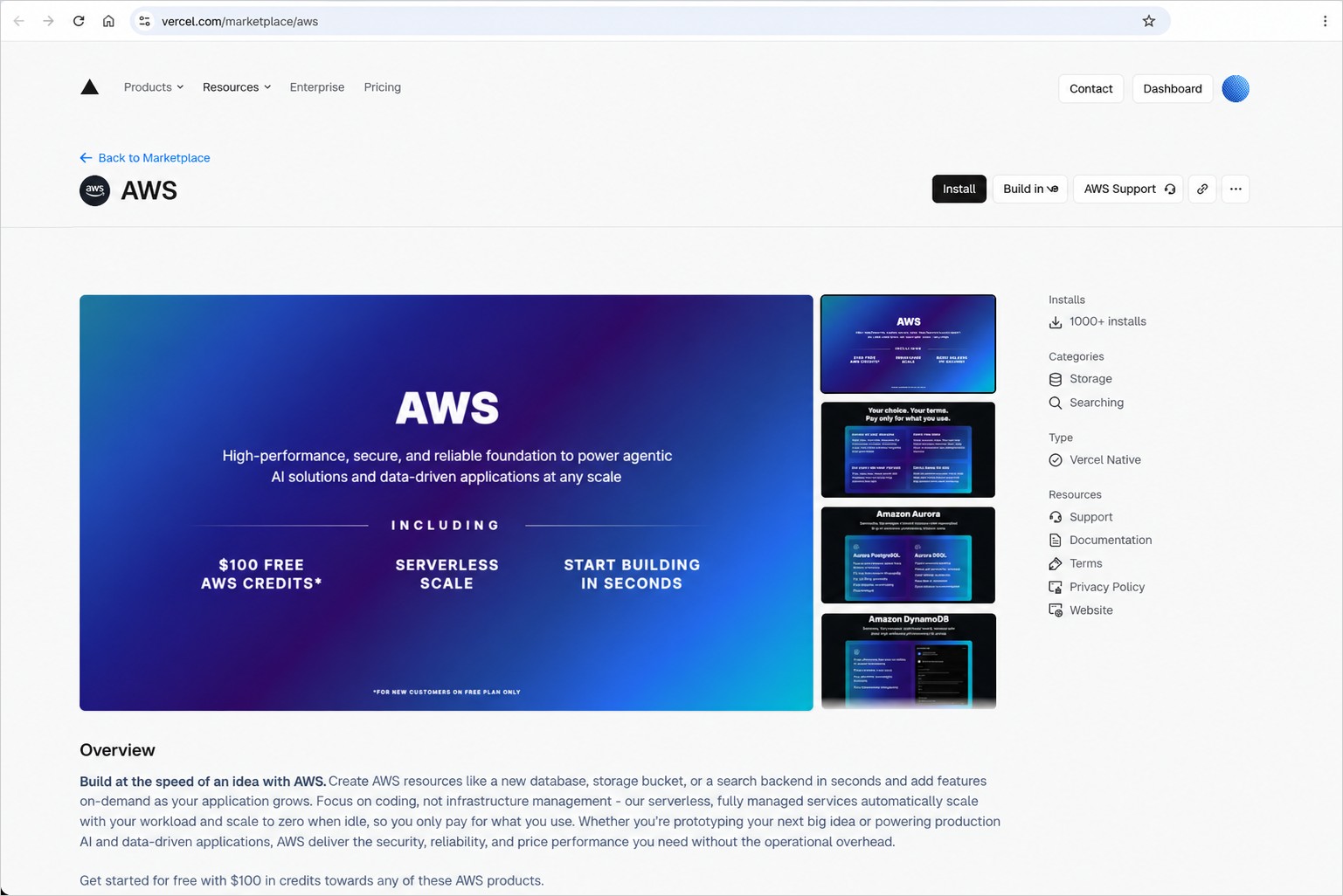
AWS page on the Vercel Marketplace with $100 in free AWS credits, serverless scale, and an Install button

Figure 1 – The AWS page on the Vercel Marketplace.

Getting started

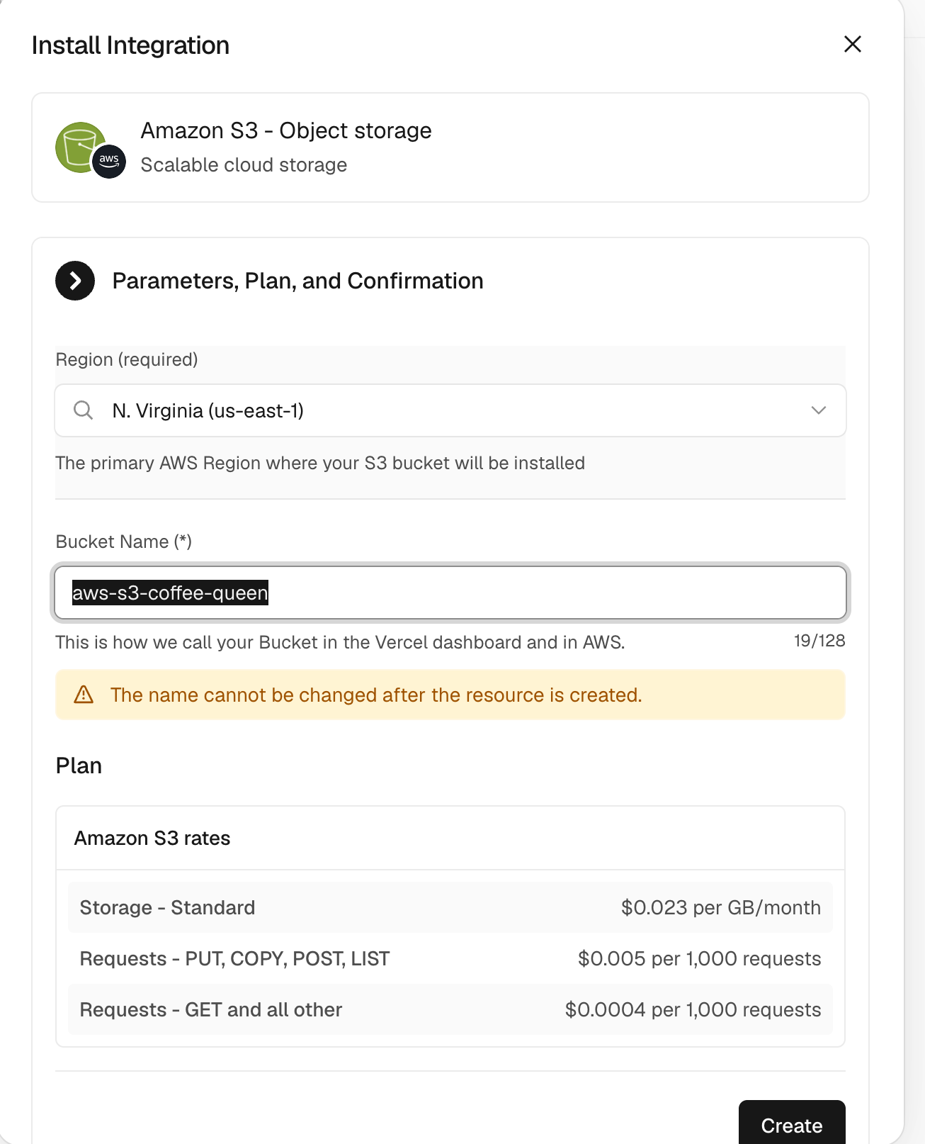
From the Vercel dashboard, go to the Storage tab and choose Create. Select AWS, pick your S3 bucket type, choose a Region, and create the bucket. Provisioning takes a few seconds.

Figure 2 – Creating an Amazon S3 general purpose bucket in Vercel by choosing a Region and a name.

Connect the bucket to a project, then pull the environment variables with the Vercel CLI:

vercel link 
vercel env pull .env.local

The integration injects AWS_REGION, AWS_ROLE_ARN, AWS_RESOURCE_ARN, and a bucket name such as S3_BUCKET_NAME, S3_TABLE_BUCKET_NAME, or S3_VECTOR_BUCKET_NAME. At runtime, the awsCredentialsProvider from @vercel/functions/oidc exchanges a short-lived OIDC token with AWS Security Token Service (AWS STS) for temporary credentials scoped to your resource. No static keys are stored anywhere.

Object storage with S3

This Next.js route uploads a file to a general purpose bucket:

import { S3Client, PutObjectCommand } from "@aws-sdk/client-s3";
import { awsCredentialsProvider } from "@vercel/functions/oidc";

const s3 = new S3Client({
  region: process.env.AWS_REGION,
  credentials: awsCredentialsProvider({
    roleArn: process.env.AWS_ROLE_ARN,
  }),
});

export async function POST(request) {
  const formData = await request.formData();
  const file = formData.get("file");

  await s3.send(new PutObjectCommand({
    Bucket: process.env.S3_BUCKET_NAME,
    Key: file.name,
    Body: Buffer.from(await file.arrayBuffer()),
    ContentType: file.type,
  }));

  return Response.json({ success: true });
}

Use ListObjectsV2Command and GetObjectCommand with the same client to list and read objects.

Analytics with S3 Tables

S3 Tables offer S3 storage purpose-built for analytics and are designed to automatically optimize query performance as data volumes grow. They provide fully managed Apache Iceberg tables with automated table maintenance and compaction, and they work with any Apache Iceberg REST Catalog-compliant engine. You can use DuckDB inside a Vercel Function for lightweight queries. This example attaches the table bucket by its ARN and runs an aggregate query:

import { DuckDBInstance } from "@duckdb/node-api";
import { awsCredentialsProvider } from "@vercel/functions/oidc";

const creds = await awsCredentialsProvider({
  roleArn: process.env.AWS_ROLE_ARN,
})();

const db = await DuckDBInstance.create();
const conn = await db.connect();

await conn.run("INSTALL aws; LOAD aws; INSTALL httpfs; LOAD httpfs; INSTALL iceberg; LOAD iceberg;");

await conn.run(`
  CREATE SECRET s3cred (
    TYPE s3,
    KEY_ID '${creds.accessKeyId}',
    SECRET '${creds.secretAccessKey}',
    SESSION_TOKEN '${creds.sessionToken}',
    REGION '${process.env.AWS_REGION}'
  );
`);

await conn.run(`
  ATTACH '${process.env.AWS_RESOURCE_ARN}' AS s3tables (
    TYPE iceberg,
    ENDPOINT_TYPE s3_tables
  );
`);

const rows = await (await conn.run(`
  SELECT town_city, AVG(median_price) AS avg_price
  FROM s3tables."${process.env.S3_TABLES_NAMESPACE}".town_monthly
  GROUP BY town_city
  ORDER BY avg_price DESC
  LIMIT 10
`)).getRowObjects();

If you run DuckDB inside a Next.js route, add @duckdb/node-api to serverExternalPackages in next.config.mjs so the native bindings are not bundled.

Vector search with S3 Vectors

S3 Vectors deliver purpose-built, cost-optimized vector storage for AI agents, AI inference, and semantic search of your content stored in Amazon S3. S3 Vectors provides native support for storing and querying vectors without a separate vector database, but it does not generate them. Create the embeddings with your model of choice, then query the index for the closest matches:

import { S3VectorsClient, QueryVectorsCommand } from "@aws-sdk/client-s3vectors";
import { awsCredentialsProvider } from "@vercel/functions/oidc";

const vectors = new S3VectorsClient({
  region: process.env.AWS_REGION,
  credentials: awsCredentialsProvider({
    roleArn: process.env.AWS_ROLE_ARN,
  }),
});

export async function POST(request) {
  const { embedding } = await request.json();

  const result = await vectors.send(new QueryVectorsCommand({
    vectorBucketName: process.env.S3_VECTOR_BUCKET_NAME,
    indexName: "documents",
    queryVector: { float32: embedding },
    topK: 5,
    returnMetadata: true,
  }));

  return Response.json({ matches: result.vectors });
}

Building with v0 by Vercel

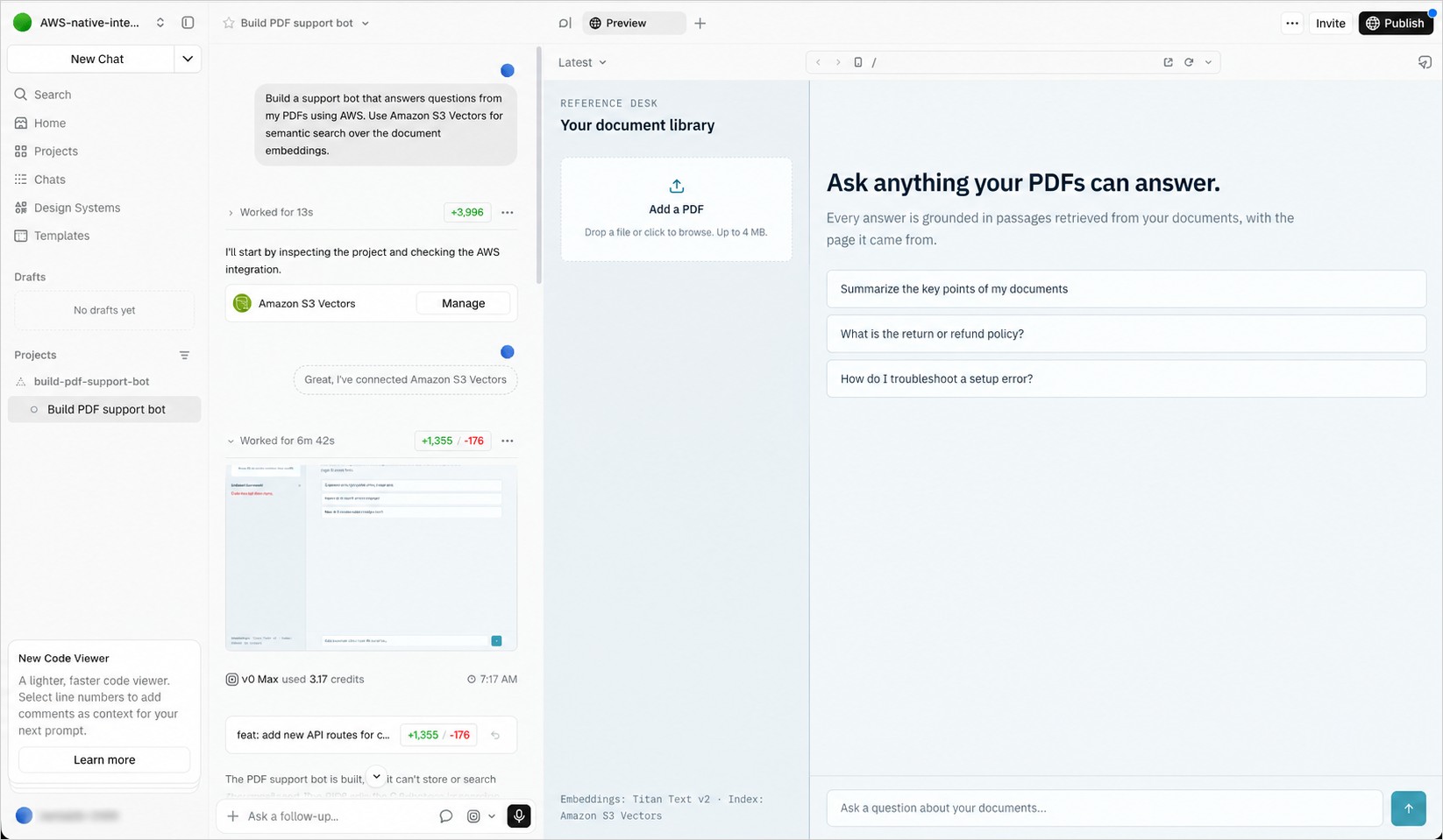
From v0, describe what you want to build and it provisions the right resource. Ask for “a photo gallery where users upload images using AWS” to get a general purpose bucket, “a support bot that answers questions from my PDFs” to get S3 Vectors, or “an analytics dashboard for my clickstream data” to get S3 Tables. v0 then configures the connection and generates working code.

v0 chat with the Amazon S3 Vectors integration connected and the generated PDF support bot application in the Preview panel

Figure 3 – v0 generating a PDF support bot from a natural language prompt, with Amazon S3 Vectors connected and the application in the Preview panel.

Combining S3 with AWS databases

Every AWS service on Vercel shares the same account and authentication model, so you can combine them with no extra setup. For example, store file metadata in Aurora with the files in S3, or store document text in DynamoDB with embeddings in S3 Vectors for RAG retrieval.

Using Vercel with your AWS account

You can create a new AWS account through the integration, which supports S3 features for building and testing. You can also link an existing AWS account to use your full set of S3 and AWS capabilities and keep your current billing. If you link an existing AWS account, Vercel works only with new buckets that you create through the platform. Because every S3 resource lives in your own AWS account, you keep AWS-native tooling and a single place to manage storage.

Pricing and availability

There is no charge for the integration, and you pay standard Amazon S3 pricing for the resources you use. New AWS accounts created through Vercel receive $100 in credits valid for six months. Amazon S3, including S3 Tables and S3 Vectors, is available from v0 and the Vercel Marketplace in all commercial AWS Regions supported by Vercel. To get started, visit v0 or the AWS page on the Vercel Marketplace.

Join the conversation

If you want to call APIs, search documentation, find regional availability, and check troubleshooting about this new feature, try using the AWS MCP Server and plugins with your preferred AI tool. Share your feedback on AWS re:Post for Amazon S3.

— Daniel

From 2,500 requests to 24: Rebuilding star history without the stargazers

Post Syndicated from Taylor Cuilty original https://github.blog/engineering/architecture-optimization/from-2500-requests-to-24-rebuilding-star-history-without-the-stargazers/


Maintainers look at star history to answer a practical question: did a launch, release, or event change a project’s trajectory? To reconstruct that curve from the GitHub API, tools had to request pages of stargazer records (each person who currently stars the repository and when they starred it), keep the timestamps, and throw the identities away.

Over time, that design created problems at both ends. Identities were available for bulk collection, so bad actors started scraping public stargazer lists for spam and phishing campaigns. For highly starred repositories, the endpoint could also make the database process many thousands of entries to return a single page.

The fix seemed clear: return counts instead of people. But returning less data didn’t actually make the query any cheaper.

Now maintainers have a direct way to get the curve: we built an endpoint that returns up to 30 weeks of daily star counts in a single request, with no identities attached. Keeping that cheap to serve meant reducing how much data the database processed, not just how much it returned, and the endpoint does that by filtering stars by time before it counts anything.

What maintainers need from star history

We first addressed the immediate risks to developers and to our database by restricting stargazer and watcher lists to repository administrators and collaborators. After the access change, callers without the required permission could receive an empty response or a 403 Forbidden response.

That change also cut off tools that had used the old response to calculate star history, often without displaying or otherwise using the usernames it returned. So we talked with maintainers and tool builders to understand what they still needed. They used star history as an approximate signal of interest: to compare activity before and after a release, or to see whether an announcement reached new developers. What they cared about was the curve.

The old API response had made identity look like part of that contract because every timestamp arrived attached to a user. In practice, tools such as Star History needed counts and dates, not usernames or other user data. Once identity was no longer part of the requirement, we could design an aggregate endpoint for the actual job: retrieving changes in star counts over time at a useful resolution.

When the API change disrupted Star History, users rallied around the project. GitHub’s Community team listened and connected us with product engineering, who dug into our use case and worked alongside us to design a purpose-built endpoint. A difficult situation became a constructive collaboration between GitHub, Star History, and the broader community—ultimately leading to a better solution.

Tianzhou Chen, star-history.com maintainer and Bytebase co-founder

Why the original endpoint was expensive

Once we knew what maintainers needed, the next step was understanding why the original design couldn’t provide it cheaply. The original GET /repos/{owner}/{repo}/stargazers endpoint was built to answer a simple question: who starred this repository? It returned a paginated list of people, and if the request specified a custom media type, each entry also included when the star was created.

The star model was built for the same job. It records the current set of people who have starred a repository, which keeps showing a star count or a list of stargazers simple. It was not designed as a historical event log: when someone removes a star, that record is removed. When tools began using the list as a time series, reconstructing a growth curve meant retrieving individual identities and processing every current star. Because each page held at most 100 people, the work grew with the repository’s popularity: building the full curve for react/react, with about 251,000 stars, took about 2,511 requests, so tools often ran into rate limits or sampled pages instead of reading them all.

Serving a page required the database to query the repository’s current stars. Due to a bug in the pagination implementation, every request also counted all of those stars to work out how many pages existed, even though the caller received only one page of up to 100 people. On a highly starred repository, that meant counting many thousands of entries on every request. In the week before we restricted access, nearly 37,000 of these count queries ran slowly enough to be logged, averaging nearly 3 seconds each, and database safeguards killed more than 1,000 of them, which contributed to request timeouts.

The chart below shows what all that counting cost. After we restricted access, the database served about 60% fewer stargazer requests, and the total time it spent on the count query fell by about 80%.

Approaches we considered

Removing identities handled the privacy requirement. The harder part was keeping each request from scanning the repository’s entire current star set.

Keeping events without identities

Our first spike kept one record per star and returned the starred_at value without the stargazer’s identity for callers who lacked collaborator access. At first, this looked like the quickest path forward, because it directly served the request we had heard from tool builders. It also closed the identity-harvesting path with a relatively small change to the existing serialization and authorization flow.

This approach addressed identity exposure and would have allowed existing tools to keep working. But API consumers would still have to paginate through and process potentially many thousands of individual records to build an aggregate history. It also tied the new use case to an endpoint and pagination model designed for listing people rather than retrieving trends.

Aggregating, then paginating

Aggregation seemed like the obvious next step. Instead of returning one row per star, the query could group stars into daily or weekly buckets, sort those buckets, and paginate the much smaller result.

The problem was where pagination happened. In a straightforward SQL query, the database first finds all stars for the repository, groups them into buckets, and sorts those buckets. Only then does it apply LIMIT, which controls how many buckets are returned, and OFFSET, which determines where the page begins:

all matching stars -> bucket every row by day or week -> sort every bucket -> OFFSET/LIMIT -> response

For a popular repository, an anonymous request could still scan and aggregate many thousands of index entries to return a handful of buckets. Returning fewer buckets would shrink the JSON response, but it would not reduce the expensive grouping and sorting the database had already performed. For react/react, reading the full history that way would have meant examining roughly 6 million rows, because every one of the 24 requests would have reprocessed all of its stars. To reduce the query cost, we had to narrow the rows before aggregation began.

Filtering by time before grouping

The design we shipped paginates star history by calendar week. For each request, it translates page and per_page into an indexed created_at range, filters the stars to those weeks, and then groups the matching records into daily counts. A response includes up to 30 weeks, and increasing page moves backward through the repository’s history.

indexed date range -> group rows in that range -> daily buckets -> response

With the date range applied first, each request processes the weeks being returned instead of every current star in the repository. For tools, that means one request now covers up to 30 weeks of history, no matter how many stars the repository has. For react/react, that’s about 24 requests instead of about 2,511, and the database examines each star about once (roughly 251,000 rows) across the full history. This fits the primary use case because maintainers usually inspect growth across weeks or around a known release, launch, or event. Week-based ranges also align with other repository activity APIs: the response follows the same shape as the weekly commit activity endpoint, GET /repos/{owner}/{repo}/stats/commit_activity.

The time-range design limits each request to a defined period, but it does not limit the number of stars within that range. A week with an unusually large number of stars can therefore still produce a slow or expensive query. The normal request path no longer queries every current star, but exceptionally dense weeks remain a scaling limitation.

Comparing the performance of the old and new API paths also surfaced other places where GitHub was counting stars on demand. We found the same pattern on the repository stargazers page on GitHub.com and updated it to use the repository’s cached star count. Slow queries from that page, which had numbered in the hundreds each week, dropped to zero. We recently shipped a similar fix to other stargazer API endpoints.

The chart below shows slow and killed stargazer count queries each week, by where they came from.

What we learned

  1. A smaller response does not always mean a cheaper query. LIMIT and OFFSET reduced the number of results returned, but they did not reduce the grouping and sorting the database had already done. We had to look at the order in which the work happened.
  2. Start with what people are actually trying to do. Maintainers needed to compare trends. A list of identities was simply how the old endpoint happened to provide the underlying data.
  3. Return only what the use case needs. Anything more is data someone else can misuse. Once we understood the job, we could remove individual identities without taking away the information maintainers relied on.
  4. Be clear about the tradeoffs that remain. The new endpoint is safer and more predictable, but calendar boundaries, removed stars, and unusually dense weeks still affect what it can return. Those details are part of the API contract too.

Restricting the original endpoint addressed the immediate problem. Listening to maintainers gave us something better than what we started with: star history that’s easier to get, cheaper to serve, and safer for everyone who stars a project.

Get repository star history, then share feedback in the GitHub Community discussion.

The post From 2,500 requests to 24: Rebuilding star history without the stargazers appeared first on The GitHub Blog.

Your serverless attendee’s guide to AWS re:Invent 2026

Post Syndicated from Nicolas Tarzia original https://aws.amazon.com/blogs/compute/your-serverless-attendees-guide-to-aws-reinvent-2026/

AWS re:Invent 2026 offers an extensive selection of serverless and application integration content. This year’s lineup includes new AWS Lambda execution models: durable functions, Lambda Managed Instances, and Lambda MicroVMs. It also covers AI agents as a new kind of serverless consumer and maturing patterns for production event-driven applications.

Don’t have a ticket yet? Register for re:Invent 2026 and join us in Las Vegas from November 30 to December 4.

For detailed descriptions and schedule, visit the AWS re:Invent Session Catalog. Sessions are held across several venues, so allow extra time to travel between properties.

We’ve curated this guide to help you navigate the serverless sessions and find the content most relevant to you.

Session types

  • Breakout Sessions are lecture-style presentations covering architecture, best practices, and deep dives into AWS services.
  • Workshops are 2-hour hands-on sessions where you work through tasks in AWS accounts using AWS services. Laptops are required.
  • Chalk Talks are highly interactive 60-minute sessions with smaller audiences, focused on technical deep dives with whiteboards for architectural discussions.
  • Builders’ Sessions are 60-minute small-group sessions led by an AWS expert who guides you through a technical problem using AWS services.
  • Code Talks are 60-minute live coding sessions where AWS experts show how to build solutions using AWS services.
  • Lightning Talks are 20-minute sessions focused on a single idea.

What’s new in AWS Serverless

Start here to get oriented on what has changed in serverless heading into re:Invent 2026.

SVS207 | Modernizing your compute stack with Lambda’s new execution models – Breakout Session

Choose a Lambda execution model for each workload class, run mixed deployments, and compare monitoring across models. Bring your workload portfolio.

SVS305 | What’s new in AWS Serverless – Workshop

Build with the newest serverless releases and work through the trade-offs that matter in real systems.

SVS339 | What’s new with Amazon API Gateway – Breakout Session

See what’s new in Amazon API Gateway, including direct service integrations that replace Lambda glue code. Learn how to design APIs for both developers and AI agents, including Model Context Protocol (MCP) servers.

Getting started with serverless

Are you new to serverless or taking your first steps? These sessions cover fundamentals and hands-on introductions.

SVS202 | Building your first event-driven application – Builders’ Session

Build a retail order system on Amazon EventBridge, Lambda, and Amazon DynamoDB where each step runs independently and one failure doesn’t cascade. No event-driven experience required.

SVS301 | AWS Serverless developer experience – Workshop

Build a realistic serverless solution while covering event-driven principles, observability, open-source tools, and deployment automation, in Python, TypeScript, Java, or .NET.

SVS302 | Building serverless applications with Terraform – Workshop

Define, deploy, and maintain serverless architectures with Terraform, including reusable modules, state management, and deployments across environments.

New Lambda execution models

Three Lambda execution models cover different workload shapes: durable functions, Lambda Managed Instances, and Lambda MicroVMs.

Lambda durable functions

API314 | A closer look at AWS Lambda durable functions – Chalk Talk

Learn how checkpointing and replay-based recovery work, see patterns such as sagas, fan-out/fan-in, and human-in-the-loop waits, and get a framework for choosing between durable functions and AWS Step Functions.

API316 | Coding an AI agent from scratch with AWS Lambda durable functions – Code Talk

Build an AI agent from scratch with durable functions, including a tool-use loop, retries with exponential backoff, and human approval that doesn’t bill for idle time.

SVS325 | Distributed transactions with Step Functions and durable functions – Builders’ Session

Build a payment processing flow with the saga pattern, using Step Functions and durable functions for compensation when part of a transaction fails.

Lambda Managed Instances

SVS332 | Lambda Managed Instances: Always-on serverless compute – Chalk Talk

Lambda Managed Instances offer Amazon Elastic Compute Cloud (Amazon EC2) economics with multi-concurrency while Lambda manages instance lifecycle, patching, and scaling. Model your break-even point, and bring your Lambda bill.

Lambda MicroVMs

SVS307 | Running untrusted code in sandboxes with AWS Lambda MicroVMs – Builders’ Session

Build sandboxes that run untrusted code, such as AI-generated code and third-party plugins, with resource limits, permission boundaries, and tested failure modes.

SVS337 | AWS Lambda MicroVMs: Strong isolation for agents and beyond – Breakout Session

Learn how Lambda MicroVMs work: VM-level isolation per agent, tenant, or task, with state that persists across invocations and sandboxes that suspend when idle and resume on demand.

Serverless and AI agents

A major theme this year is building, orchestrating, and operating AI agents on serverless infrastructure.

SVS338 | Serverless developers in the agentic era: What changes, what doesn’t – Breakout Session

See what changes when AI agents call your functions as tools, and what stays the same. Topics include orchestration for non-deterministic workflows and cost governance when one reasoning chain calls 200 functions.

SVS306 | Building agentic AI architectures with AWS Serverless – Builders’ Session

Build a multi-agent system that uses Lambda for tool execution, Amazon Bedrock for reasoning, and Amazon EventBridge for communication between agents.

SVS324 | Building agentic apps with serverless: Lambda as your agent’s toolbox – Chalk Talk

Design Lambda functions as agent tools, with single-responsibility tools, clear input and output schemas, MCP-compatible interfaces, and multi-tenant isolation.

SVS342 | Coding the tool layer for AI agents on serverless – Code Talk

Retrofit a serverless API into an agent tool, live. The build covers an MCP server with versioned tools, discovery through the Gateway capability of Amazon Bedrock AgentCore, a Step Functions workflow exposed as one tool, and scoped agent identity.

API312 | Building event-driven, multi-agent architectures on serverless – Chalk Talk

Map agent coordination patterns on Amazon EventBridge, such as peer-to-peer messaging, supervisor-worker hierarchies, and broadcast, and the failure modes they introduce, including circular delegation.

COM325 | The agent orchestration spectrum: agents, Step Functions, or Lambda? – Code Talk

Live-code the same AI workload with AgentCore, Step Functions, and durable functions, and compare latency, cost, and debuggability on a production content platform.

SVS328 | Guardrails for AI-generated serverless infrastructure – Chalk Talk

Coding agents can generate over-permissioned AWS Identity and Access Management (IAM) policies and skip encryption. Learn which guardrails to automate and which need human review.

API402 | Building event-driven architectures in the age of AI agents – Breakout Session

See how familiar patterns such as queues, events, and retries evolve when your consumers are autonomous agents instead of microservices.

Building event-driven architectures

Event-driven architectures remain the backbone of serverless applications. These sessions cover patterns from foundational to advanced.

API302 | Serverlesspresso: Build an event-driven app from the ground up – Workshop

Build a serverless coffee-ordering app with Lambda, Amazon EventBridge, and durable functions, which checkpoint progress and recover from failures without custom state management.

API305 | Building enterprise-scale event buses with Amazon EventBridge – Builders’ Session

Configure an event bus with routing policies, schema discovery, and access controls so platform teams govern events while application teams ship independently.

API311 | How event-driven architectures go wrong and how to fix them – Chalk Talk

Dissect costly anti-patterns such as unbounded fan-out, missing dead-letter queues, chatty event schemas, and orchestration gaps that silently drop work, and fix them.

API317 | Coding event-driven retry patterns that prevent outages – Code Talk

Live-code exponential backoff with jitter, circuit breakers, poison-pill isolation, and replay from archive for Amazon EventBridge and Step Functions.

Orchestration: Step Functions and durable functions

Both Step Functions and Lambda durable functions handle retries, long-running execution, and failure recovery. These sessions help you choose.

API318 | Composing the right orchestration for serverless workflows – Lightning Talk

A decision framework for human approvals, long-running AI agent workflows, and multi-service sagas, plus a hybrid pattern that uses durable functions inside Step Functions.

ARC329 | The coordination decision: when to orchestrate and when to let go – Breakout Session

Decide per flow whether to orchestrate or let services react to events, using a logistics platform that runs both patterns on Step Functions and Amazon EventBridge.

Building APIs and serverless web applications

Serverless is increasingly used to build full-stack web applications, not only API backends.

SVS348 | Serverless compute built for the web – Breakout Session

Build full-stack web applications entirely on serverless services, with patterns for HTTP routing, server-side rendering, static assets, and real-time features.

SVS327 | Build interactive web apps with AWS Lambda – Chalk Talk

Run web frameworks such as Express, Hono, and Next.js on Lambda with runtime adapters, including migration paths for containerized web apps.

API304 | API Gateway unleashed – Workshop

Create, deploy, and manage APIs with API Gateway, including message transformation, request validation, security, Infrastructure as Code, and WebSocket backends.

API306 | Build secure APIs faster with Amazon API Gateway and Kiro CLI – Builders’ Session

Implement and compare API Gateway authorization with Amazon Cognito user pools, Amazon Verified Permissions, Lambda custom authorizers, and IAM authorizers. Then go from spec to deployed API with Kiro CLI, OpenAPI, and MCP servers.

API309 | Amazon API Gateway: Migration strategies and agent-ready APIs – Chalk Talk

Learn migration strategies from legacy API platforms, then design APIs that AI agents can discover, authenticate against, and call, including MCP-compatible tool definitions.

Serverless developer experience

AI-assisted development is changing how serverless applications are built, tested, and deployed.

SVS303 | AI-driven serverless development with Kiro – Workshop

Use Kiro to build a serverless application with authentication, tests, observability, and an optional continuous integration and continuous delivery (CI/CD) pipeline.

SVS343 | A day in the life of a serverless builder – Code Talk

Follow one serverless application from first line of code to production, live: an AI coding agent generates the scaffolding, and you debug a failing request with OpenTelemetry.

SVS329 | Testing serverless and event-driven applications – Chalk Talk

Whiteboard testing strategies for serverless and event-driven apps, from unit and contract tests to chaos techniques such as duplicate and out-of-order delivery.

SVS322 | Build self-healing serverless applications with AWS DevOps Agent – Builders’ Session

Inject failures such as Lambda throttling, timeout cascades, and dead-letter queue buildup, then configure AWS DevOps Agent to find root causes and apply fixes with approval gates.

Performance, cost, and operations at scale

Tune your Lambda functions, optimize costs, and learn what changes when you operate at enterprise scale.

SVS341 | Lambda performance tuning and cost optimization – Chalk Talk

Go beyond memory tuning with SnapStart and provisioned concurrency, event source mapping tuning, and guidance on when Lambda Managed Instances beat per-invocation pricing.

SVS335 | Operating serverless at scale: What changes at 1,000+ functions – Chalk Talk

Learn what changes between 10 and 1,000 functions: safe deployments, account structure and concurrency management, observability without cardinality overload, and platform patterns.

ARC325 | Serverless at 1M RPS: Lambda, DynamoDB, and SQS scaling lessons – Chalk Talk

Push Lambda, DynamoDB, and Amazon Simple Queue Service (Amazon SQS) to one million requests per second and see what breaks. The session shares real numbers on cold start budgets, retry amplification, and backpressure.

SVS334 | Serverless observability: OpenTelemetry and vended logs – Chalk Talk

Set up OpenTelemetry and API Gateway vended logs for tracing across Step Functions, Amazon EventBridge, and SQS, plus observability for agentic workloads such as token use.

SVS320 | Same code, any compute: Portable architecture on AWS – Builders’ Session

Apply Hexagonal Architecture and 12-factor patterns so compute is a deployment decision, not an architectural one, using the AWS Lambda Web Adapter and runtime-neutral handlers.

Serverless data processing

Process data at scale without provisioning clusters or managing batch infrastructure.

SVS309 | Building serverless distributed data processing workloads – Builders’ Session

Build a pipeline with Step Functions Distributed Map, Lambda, and Amazon Simple Storage Service (Amazon S3) that processes thousands of objects in parallel and handles partial failures.

SVS321 | Serverless streaming data processing with AWS Lambda and Apache Kafka – Builders’ Session

Build a real-time location tracking app that ingests events from Amazon Managed Streaming for Apache Kafka (Amazon MSK), processes them with Lambda, and updates a dashboard through AWS AppSync.

Community sessions

Sessions led by AWS community members and customers sharing production experience with the preceding execution models and patterns.

COM303 | Lambda for every scale and workload shape – Breakout Session

Honeycomb shares how it runs its query backend across all three Lambda execution models. Honeycomb reports that Managed Instances absorb steady-state traffic at roughly 7.5x lower cost than Functions, while MicroVMs take spikes and Functions catch bursts.

COM326 | Observable agents with Lambda durable functions and OpenTelemetry – Code Talk

Build a multi-agent purchasing coordinator on durable functions and instrument it with OpenTelemetry for one coherent trace across all invocations, plus Amazon CloudWatch insights for fleet-wide queries.

COM304 | Hidden trade-offs in distributed architectures – Breakout Session

Investigate unexpected system behavior in a real-world case study built on Lambda, DynamoDB, DynamoDB Streams, and Step Functions, and learn the trade-offs behind it.

Additional resources

Many sessions run more than once, so if a session is full, check the catalog for another time.

If you cannot join in person, we upload breakout sessions to the AWS Events YouTube channel after the event.

For more serverless learning resources, visit Serverless Land.

We look forward to seeing you at re:Invent 2026!

Upcoming Speaking Engagements

Post Syndicated from Bruce Schneier original https://www.schneier.com/blog/archives/2026/10/upcoming-speaking-engagements-61.html

This is a current list of where and when I am scheduled to speak:

  • I’m speaking at ATTENTION: Democracy, Rebuilt in Montreal, Canada. The event runs October 21–23, 2026, and my talk is on Wednesday, October 21.
  • I’m speaking at the University of Toronto in Toronto, Ontario, Canada, at 5 PM ET on October 22, 2026.
  • I’m speaking at [un]prompted in San Francisco, California. The event runs October 27–29, 2026, and my talk is at 11:35 AM PT on Thursday, October 29.
  • I’m speaking at the Catalyst Summit in Brampton, Ontario, Canada, on Wednesday, November 18, 2026.
  • I’m speaking at QT Qonference 2026 in Toronto, Ontario, Canada, on Thursday, November 19, 2026.

The list is maintained on this page.

Multi-region disaster recovery for Amazon API Gateway WebSocket APIs

Post Syndicated from Shubham Dhoka original https://aws.amazon.com/blogs/architecture/multi-region-disaster-recovery-for-amazon-api-gateway-websocket-apis/

WebSocket connections power some of the most interactive experiences on the web: financial trading applications streaming live market data, collaborative editing tools where multiple users work on the same document, gaming leaderboards updating in real time, and IoT dashboards monitoring thousands of devices. These applications depend on persistent, bidirectional communication between clients and servers.

Real-time applications using WebSocket connections face a unique challenge during Regional outages. WebSocket connections are persistent and bound to a specific AWS Region. A Regional failure severs every active connection. For applications that also maintain shared state across those connections, such as a live auction or collaborative editor, users lose both their connection and their session context. This post presents a design pattern for multi-Region disaster recovery with Amazon API Gateway WebSocket APIs that reconnects clients and restores state automatically during failover.

In this post, you learn how to build this pattern using Amazon Route 53 for DNS-based failover, Amazon DynamoDB Global Tables for cross-Region state replication, a canary health probe for traffic-independent failure detection, and client-side reconnection logic to recover from Regional failures while preserving application state.

Solution overview

This pattern creates an active-passive multi-Region architecture where the primary Region serves WebSocket connections and automatically fails over to a secondary Region during a disaster. The core idea is separating application state from the connection itself, so the client can restore its session after reconnection.

The architecture deploys identical WebSocket API stacks in two Regions, a primary and a secondary. Both Regions share application state through DynamoDB Global Tables, so the secondary Region is consistently ready to serve traffic. A single custom domain name fronts both Regions. Amazon Route 53 failover routing policy directs traffic to the primary Region under normal conditions. When the primary becomes unhealthy, Route 53 automatically shifts DNS resolution to the secondary Region. Clients reconnect to the same domain and resume operations without changing their configuration.

Figure 1 shows the architecture and the normal operation and failover flow.

Architecture diagram showing a client connecting through a Route 53 failover policy to the primary Region us-east-1, which runs API Gateway WebSocket, Lambda, and DynamoDB, with an Amazon EventBridge rule triggering a canary health check and a CloudWatch alarm that drives the Route 53 health check; DynamoDB Global Tables replicate to the secondary Region us-west-2 for failover

Figure 1: Multi-region WebSocket API failover architecture

  1. A user opens the application, which establishes a WebSocket connection to the application’s domain name.
  2. Amazon Route 53 resolves the domain using a failover routing policy. Under normal conditions, it returns the primary Region’s endpoint.
  3. The WebSocket connection reaches API Gateway in the primary Region, which invokes an AWS Lambda function for each connection event and message.
  4. Lambda reads and writes application state to DynamoDB. Connected clients receive updates through their open WebSocket connections.
  5. DynamoDB Global Tables replicates the application state to the secondary Region asynchronously, keeping it ready to serve traffic.
  6. Independently, an Amazon EventBridge rule triggers a canary Lambda function every minute.
  7. The canary opens a WebSocket connection to the API Gateway endpoint, sends a heartbeat, and publishes the result as a custom Amazon CloudWatch metric.
  8. A CloudWatch alarm evaluates the metric. If the canary reports consecutive failures or stops publishing, the alarm fires and the associated Route 53 health check marks the primary as unhealthy.
  9. Route 53 detects the unhealthy primary and begins resolving the domain to the secondary Region instead.
  10. Clients reconnect through the same domain, now reaching the secondary Region, and recover their application state from the local DynamoDB replica.

Prerequisites

To follow along with this post, you need:

Deploy the solution

The complete source code and deployment instructions are available on the GitHub repo. The repository includes AWS CloudFormation templates for the WebSocket APIs, canary health probe, and a React client application with the reconnection logic described in this post.

The demo application

The sample application is a real-time auction where multiple users bid on an item simultaneously. Each bid updates a shared counter through WebSocket messages, and connected clients see the current bid in real time. The application displays which AWS Region is serving responses, making failover visible during testing. Although minimal, this pattern represents real-time workloads where multiple clients share mutable state over WebSocket connections: chat applications, collaborative editors, live dashboards, or multiplayer games.

Managing connection state across Regions

WebSocket connections are persistent, but the application state built on top of them is what matters during failover. As users interact with the application, the server builds up session data tied to their identity. When a failover occurs and the client reconnects to a different Region, that session data needs to be available for the experience to continue uninterrupted. This solution stores state in DynamoDB Global Tables, which replicates it to the secondary Region asynchronously, typically within a second. Because this replication is asynchronous, writes that occur immediately before a failure may not reach the secondary Region. For most applications, this window is small enough to be acceptable.

After failover, the client reconnects and restores its state. In this demo, the client sends a getState message after reconnection to retrieve the latest application state from the secondary Region’s DynamoDB replica.

Production applications add two considerations on reconnection. First, clients authenticate again: WebSocket APIs authenticate on the $connect route, so after failover the secondary Region re-authenticates the client through a Lambda authorizer. Deploy that authorizer in both Regions so reconnecting clients can authenticate against either one. Second, to restore state, identify the user from the validated token, such as the sub claim. Key the stored state by the user ID rather than the connection ID, which changes on every reconnect. Applications model session state in different ways, so adapt this to your design.

If your application uses a relational database, you need to set up similar cross-region state replication. For instance, Amazon Aurora Global Database provides sub-second replication latency across Regions. Note that Aurora requires promoting a read replica to primary during failover, which typically adds 1–2 minutes to the recovery process. This promotion can also be automated based on a CloudWatch alarm action.

Heartbeat

Both the client and the canary use application-level heartbeat to verify their WebSocket connections are alive. At a regular interval, they send a lightweight message and expect an acknowledgment. A missing or invalid response signals a broken connection. The client uses this to trigger reconnection. The canary uses it to drive the Route 53 health check. This mechanism is described in RFC 6455 and is the standard approach for WebSocket connection health monitoring.

The client code snippets in this post use react-use-websocket, a React library that provides built-in support for reconnection and heartbeat. You can implement the same patterns in other WebSocket client libraries or languages.

heartbeat: {
  message: JSON.stringify({ action: 'heartbeat' }),
  returnMessage: 'pong',
  timeout: 35000,   // Close connection if no message received within 35s
  interval: 30000,  // Send heartbeat every 30s
}

Detecting regional failures automatically

When the primary Region becomes unavailable, Route 53 needs to detect the failure and redirect traffic to the secondary. To do this, the solution creates a health check that actively monitors the WebSocket endpoint. A Lambda function called the canary, deployed in the primary Region, powers this health check. It probes the endpoint every minute by opening a WebSocket connection, sending a heartbeat message, and confirming it receives a valid response. The canary publishes the result as a custom CloudWatch metric (App/WebSocketHealth, dimension ApiId): 1 for healthy, 0 for unhealthy.

A CloudWatch alarm monitors this metric and treats both failures and missing data as unhealthy (TreatMissingData: breaching). After two consecutive unhealthy datapoints, the alarm fires and the associated Route 53 health check (configured with InsufficientDataHealthStatus: Unhealthy) marks the primary as down. Route 53 shifts DNS to the secondary Region.

Failback works through the same mechanism. When the primary recovers, the canary starts succeeding again, the alarm clears, and Route 53 shifts traffic back. For production workloads, consider asymmetric thresholds: use a low threshold (two datapoints) for fast failover and a higher threshold (over five) for slower failback, which helps prevent flapping if the primary is unstable during recovery. A DNS time-to-live (TTL) of 60–120 seconds provides a good balance between fast propagation and lookup efficiency.

Client reconnection strategy

When a connection drops, the client needs to reconnect without overwhelming the recovering service. The heartbeat described earlier handles detection in most cases. If no messages arrive within the timeout window, the library closes the connection. However, the backend can be degraded rather than fully unreachable. For example, API Gateway returns error responses when the Lambda function is throttled, so the connection remains technically open while the application is non-functional. To handle this, the client tracks consecutive failed heartbeats: responses that aren’t the expected pong message. After 2 consecutive failures, the client force-closes the connection and triggers reconnection. With a 30-second heartbeat interval, this detects a degraded backend within 60 seconds.

After the client identifies a broken connection, it begins reconnecting using exponential backoff with full jitter, a pattern described in the AWS Architecture Blog post Exponential Backoff And Jitter. The reconnection interval doubles with each attempt, and full jitter randomizes the actual delay within that window. This spreads reconnection attempts over time, helping prevent a thundering herd where many clients retry simultaneously and overwhelm the secondary Region the moment DNS shifts.

reconnectInterval: (attempt) => {
  // Exponential backoff with full jitter
  const expDelay = Math.min(2000 * Math.pow(2, attempt), 20000);
  return Math.random() * expDelay;
}

After each successful reconnection, the client requests the current application state from the server. Because the client reconnects to the same custom domain, Route 53 resolves it to whichever Region is currently healthy. The client doesn’t need to know which Region it’s connecting to. The server includes the Region in its response, and the application can update its UI or logging accordingly.

Failover in action

To see the full failover sequence, start the client application and connect to your WebSocket endpoint:

cd client
cp .env.example .env.local
# Edit .env.local with your custom domain URL
npm install
npm run dev

Open the application in your browser and note the serving Region displayed in the UI.

Auction app showing Connected status and serving Region US-EAST-1 with a current bid of $9

Figure 2: Client connected to the primary Region (us-east-1)

Next, simulate a failure by setting the primary Lambda function’s reserved concurrency to zero, which prevents it from processing requests:

aws lambda put-function-concurrency \
  --function-name counter-handler-us-east-1 \
  --reserved-concurrent-executions 0 \
  --region us-east-1

Within about two minutes, the canary detects the failure after two consecutive failed probes at one-minute intervals. Route 53 then marks the primary as unhealthy, and DNS begins resolving to the secondary Region.

The client detects the dropped connection and begins retrying with exponential backoff and jitter.

Auction app showing Disconnected status and reconnecting after a connection failure, with connection errors in the activity log

Figure 3: Client detecting failure and reconnecting with exponential backoff

When DNS propagation completes, the next reconnection attempt reaches the secondary Region. The client requests the current state, recovers it from DynamoDB Global Tables, and the UI updates to show the new serving Region.

Auction app reconnected to serving Region US-WEST-2 after DNS failover, with the current bid of $9 preserved

Figure 4: Client after failover to the secondary Region (us-west-2) with state preserved

When the primary Region recovers, the canary confirms that it’s healthy again. After the alarm clears, Route 53 shifts DNS back and clients reconnect to the primary through the same automatic process. No manual intervention is needed for failback.

Clean up

To avoid ongoing charges, delete the resources created during this walkthrough:

  1. Delete the CloudFormation stacks:
    aws cloudformation delete-stack --stack-name websocket-health-check --region us-east-1
    aws cloudformation delete-stack --stack-name websocket-counter-secondary --region us-west-2
    aws cloudformation delete-stack --stack-name websocket-counter-primary --region us-east-1

  2. Delete the Route 53 failover records and API Gateway custom domain names manually from the console.

Conclusion

In this post, you learned how to build a multi-region disaster recovery pattern for API Gateway WebSocket APIs. By separating application state from the connection itself, you can restore sessions automatically after a regional failover. This pattern applies to real-time applications where WebSocket continuity matters. Adapt the health check thresholds, reconnection timing, and state recovery approach to fit your workload.

To learn more about the services used in this solution, refer to the following resources:


About the authors

How UTS established a modern curriculum data services foundation on AWS

Post Syndicated from Oleg Polianski original https://aws.amazon.com/blogs/architecture/how-uts-established-a-modern-curriculum-data-services-foundation-on-aws/

Students and staff experience the University of Technology Sydney (UTS) as a single institution, not as the collection of curriculum and student systems behind it. They expect the information underpinning teaching, learning, course design and institutional decision-making to be accurate, timely and coherent, irrespective of its source.

Behind that experience, UTS had reached a natural inflection point in its integration landscape. Critical teaching and learning capabilities relied upon established vendor platforms with disparate data models, interfaces, stability profiles and scaling characteristics. Although those platforms continued to perform essential operational functions, integrating and operating the surrounding estate had become progressively more intricate and costly.

UTS’s purpose remained constant: excellence in teaching, learning and the student experience. Technology exists to advance that purpose, not to supplant it. UTS Information Technology Unit (ITU) therefore sought to remove impediments between authoritative data and the people, processes and digital services that depend upon it.

UTS made that transition practical with AWS. With managed, elastic and serverless capabilities, UTS reduced undifferentiated operational effort and improved fault tolerance. This established a sustainable model for governed data services. Curriculum became the first bounded business domain in which UTS applied that model.

The challenge

UTS ITU required an architecture that could:

  • Make authoritative curriculum information available through reusable services without displacing the Curriculum Management System, a third-party software as a service (SaaS) application, as the system of record.
  • Replace tightly coupled, consumer-specific interfaces with governed contracts that insulate consumers from source schemas and implementation detail.
  • Accommodate routine change and transient high-volume activity, including complete domain reloads, without permanently provisioned capacity.
  • Support graph traversal across deeply nested and inverse curriculum relationships, exact and full-text retrieval, and semantic discovery from the same authoritative source.
  • Operate reliably and economically within finite engineering capacity whilst establishing a repeatable pattern for subsequent data domains.

Domain boundaries were non-negotiable. Curriculum describes what the university teaches and remains the responsibility of the Curriculum Management System. Preserving that bounded context prevents ownership, validation and governance from migrating into non-authoritative services.

A domain-oriented approach

UTS ITU organised the capability according to domain-driven design. Rather than aligning data services with the applications that produce or consume data, they aligned them with:

Each data product has explicit ownership, consumers, quality expectations, interface contracts and lifecycle management. Institutional data is therefore treated as a governed asset designed for reuse, not an incidental application by-product.

Declarative architecture as code provides the executable realisation of the design and a reproducible source of truth. Configuration is separated from implementation where practicable, delivery is automated and managed AWS services are preferred to bespoke infrastructure software. The discipline is “just enough code”: engineering effort focuses on building differentiated domain logic (the business rules and data services unique to higher education) rather than undifferentiated infrastructure.

Stateless execution, asynchronous communication, purpose-built persistence and independently recoverable components avoid a tightly coupled failure domain. Consumption-based services align expenditure with workload demand instead of maintaining an estate permanently sized for intermittent peaks.

Solution overview

The architecture comprises five layers: edge, ingestion, persistence, application and business logic, and interface. Each layer has discrete responsibilities, as shown in Figure 1.

Identity, encryption, network controls, observability and operational governance apply across the stack. Curriculum data services capture complete changes from the Curriculum Management System as events, preserve them in a durable event log, materialise purpose-built representations and expose governed synchronous and asynchronous services.

Five-layer UTS curriculum data services architecture connecting the Curriculum Management System through the edge, ingestion, persistence, applications, and interface layers to consumers, with observability and security spanning all layers

Figure 1: UTS curriculum data services layered architecture

The next five sections examine each layer of the realised architecture in turn.

Edge layer

The edge layer is the controlled ingress boundary between the SaaS Curriculum Management System and the curriculum domain. Its remit is deliberately narrow: receive a complete curriculum change, establish the internal event contract and submit it to the ingestion layer with minimal processing.

The source system sends change events to an Amazon API Gateway HTTP API, which invokes an AWS Lambda function acting as a technical adapter because no suitable managed connector satisfies the source system’s proprietary API contract and payload format (for example, vendor-specific REST endpoints, authentication schemes, and data structures). The adapter encapsulates the complete vendor event in a CloudEvent envelope, appends UTS operational metadata and publishes it to the appropriate Amazon Managed Streaming for Apache Kafka (Amazon MSK) Serverless topic.

The edge neither reinterprets curriculum nor performs validation or consumer-specific transformation. Validation remains within the system of record. This preserves source fidelity, prevents downstream concerns from contaminating the ingress boundary and allows the stateless edge to scale automatically during complete domain reloads.

Ingestion layer

Amazon MSK Serverless forms the durable, append-only event backbone. Curriculum changes are segregated into domain-aligned topics by academic item type, retaining the complete source event whilst allowing independent consumers to progress, retry and recover without obstructing one another.

MSK Serverless scales on demand. Routine changes consume little capacity. A domain reload fans out across the event backbone and parallel processors, then contracts after completion. Model or schema changes can be accommodated through idempotent reprocessing or a complete reload, without introducing a second curriculum authority.

Persistence layer

The persistence layer uses purpose-built data services selected according to the access patterns and business questions each representation must support. Amazon Neptune Serverless stores curriculum structures and inverse relationships as a property graph, whilst Amazon OpenSearch Service stores complete source documents and indices for exact, full-text and vector retrieval.

In Neptune, programmes of learning, areas of learning and units of learning are connected academic items. Consumers can traverse from a programme to its constituent structures or begin with a unit and identify every programme and area through which it is taught. These inverse enquiries are native graph traversals rather than application-specific joins repeatedly reconstructed by consumers.

Property graph in Amazon Neptune showing programme, major, and subject nodes connected by TEACHES and IS_TAUGHT_BY relationships

Figure 2: Curriculum structures relationships in Amazon Neptune

OpenSearch provides exact lookup, filtering and document retrieval alongside k-nearest-neighbour vector search. Selected data processors implemented as AWS Lambda functions invoke an embedding model through Amazon Bedrock and append vector representations of relevant curriculum text before persistence. Curriculum can consequently be discovered by semantic proximity rather than lexical coincidence. UTS also validated multilingual retrieval against English-language curriculum content.

Neptune and OpenSearch are independently and eventually consistent. Failure of one materialisation doesn’t block another, and neither store is exposed directly to consumers. Both are disposable projections rather than competing systems of record and can be reconstructed from the Curriculum Management System through a complete reload. Data is encrypted with a dedicated domain AWS Key Management Service (AWS KMS) key whose use is restricted to authorised domain services.

Applications layer

The applications layer converts those materialisations into reusable domain capabilities. Dozens of narrowly scoped Lambda-backed services query Neptune or OpenSearch, whilst persistence remains private and is exposed solely through governed contracts.

Amazon EventBridge Pipes acts as a set of transport adapters between MSK Serverless and the Lambda functions acting as processors and services consuming the event stream. Pipes provide routing and delivery, not curriculum validation, enrichment or business transformation, keeping processing responsibilities explicit, independently deployable and observable.

Stateless Lambda function execution allows services to scale with demand and recover independently through retries and re-invocation. Signature Version 4 (SigV4) authentication and fine-grained AWS Identity and Access Management (IAM) roles provide least-privilege access to Amazon Neptune and Amazon OpenSearch Service without distributing or managing database credentials. The services provide authoritative retrieval, graph traversal and semantic discovery without transferring responsibility for curriculum validity into the data domain.

Interface layer

The interface layer provides pull-based access through REST and GraphQL and push-based delivery of domain events, whilst keeping persistence and implementation private. Amazon API Gateway supplies the REST boundary. AWS AppSync provides GraphQL access to frequently consumed capabilities with attribute-based access control at schema level. Both interfaces invoke the same governed service contracts.

Approved consumers might also receive curriculum events in the internal CloudEvent envelope. Amazon EventBridge Pipes manages last-mile delivery without bespoke routing middleware, and consumers determine which academic item events are relevant rather than UTS maintaining a filtered stream for each consumer.

Amazon Cognito authenticates approved external consumers through OAuth 2.0 and OpenID Connect, whilst AWS native workloads use IAM. AWS Key Management Service, AWS Secrets Manager, AWS WAF, and AWS Certificate Manager provide encryption, secrets management, perimeter protection and certificate lifecycle management. Amazon Route 53 supplies naming for a single shared vanity domain, and Amazon CloudWatch and Amazon Simple Notification Service (Amazon SNS) provide observability, telemetry and targeted alerting across the architecture.

Full solution architecture

The following diagram shows the complete solution architecture, including the identity, encryption, network, observability and governance controls that apply across all five layers.

End-to-end architecture of the UTS curriculum data services solution across the edge, ingestion, persistence, application, and interface layers, with the security, operational, and ancillary services that span them

Figure 3: End-to-end architecture of the curriculum data services solution

Results and measurable outcomes

The outcome isn’t a replacement for the Curriculum Management System as the system of record. It’s a governed data foundation that leaves the system of record authoritative whilst making curriculum information reusable through APIs, graph traversal, semantic search and event delivery. Since the production launch in November 2024, the domain has recorded zero production incidents.

  • Latency – Changes become available to downstream consumers in an average of 1.6 seconds from crossing the edge layer, through synchronous and asynchronous interfaces.
  • Curriculum graph – The domain models 43,794 relationships across approximately 800 programs of learning, 3,500 units of learning and 2,500 areas of learning.
  • Consumer adoption – 11 institutional consumers have adopted the services, replacing bespoke point-to-point integrations with reusable, governed contracts.
  • Operational footprint – One engineer operates the domain. Managed, serverless and self-healing components make routine intervention negligible and remove the need for dedicated Level 3 support.
  • Cost efficiency – UTS achieved a material reduction in the total cost of ownership of curriculum data integration and delivery, consolidating capabilities previously spread across commercial products, bespoke integrations, databases and multiple support teams.
  • Availability and resilience – The platform operates continuously and has maintained downstream access to trusted curriculum information when the upstream system of record was unavailable.

Collectively, these outcomes show how a small engineering contingent can operate an institutional-scale data domain using managed AWS services, whilst increasing capability, reducing operational complexity and aligning expenditure with demand.

What’s next

The curriculum domain validated the production architecture and operating model. The student data domain followed, providing a single governed point of access for student profiles, admissions, offers, enrolments and related information. UTS is now preparing the learning activities domain, a substantially larger capability built around a lifelong learner graph using Amazon Neptune and Amazon Neptune Analytics, extending the same domain-driven pattern across the teaching and learning landscape.

Each bounded context can select the AWS services appropriate to its business questions whilst retaining common controls for identity, security, observability, delivery and operational sustainability.

Conclusion

UTS’s integration landscape had reached the point at which cumulative complexity and operational overhead constrained institutional change. The response was not technology for its own sake. UTS ITU used AWS to remove the impediments between authoritative institutional data and the teaching, learning and administrative capabilities that depend upon it.

The significance of AWS extended beyond technology selection, but the outcome was principally an architectural and operating-model achievement by UTS. Curriculum data services became UTS’s first production data domain. UTS combined domain-driven design, asynchronous processing, purpose-built persistence and governed interfaces with managed AWS capabilities that made those patterns practicable at institutional scale.

The resulting service foundation supports event streaming, graph traversal, document and semantic retrieval, compute, identity, security and governed data exposure. UTS operates it without a conventional infrastructure estate. This allowed UTS ITU to convert an ambitious architectural design into a sustainable production capability whilst keeping engineering effort concentrated on domain services rather than undifferentiated infrastructure.

Curriculum data services embody the resulting transition: from a burdensome integration model to a domain-aligned data foundation that’s reusable, resilient and operationally sustainable. UTS now possesses a repeatable model through which institutional data can be treated as a strategic asset rather than a by-product of individual systems. The university will continue to operate many systems. Students and staff should never experience the boundaries between them.

For more information or support, contact the AWS Public Sector team.


About the authors

The Future of AI Cryptanalysis

Post Syndicated from Bruce Schneier original https://www.schneier.com/blog/archives/2026/10/the-future-of-ai-cryptanalysis.html

Matthew Green has been writing a rather pessimistic series of posts about the potential for AI systems to vastly outperform humans in cryptanalysis of both symmetric and public-key ciphers.

I am more optimistic than he is. That is, I have stronger faith in the over-engineering cryptographers tend to do. I am trying to write this up in more detail.

Cyberattack on Connected Fridges in France

Post Syndicated from Bruce Schneier original https://www.schneier.com/blog/archives/2026/10/cyberattack-on-connected-fridges-in-france.html

Another IoT cyberattack, this one in France:

Hackers gained control of the software that regulates the temperatures of the refrigeration units, forcing some to warm to 50C (120F) overnight, according to one supermarket chain affected.

[…]

Normally, supermarket freezers go through a short period of defrosting overnight, in which temperatures rise slightly. But the hackers ordered the units to heat up and stay hot, although Danfoss did not confirm any reports about just how warm the fridges and freezers could become in that process.

Danfoss said the affected cold units were older models whose security software could not be updated to ward off a risk they had identified.

Any IoT device that can’t be updated is vulnerable. And, probably, any IoT device that can be updated is also vulnerable.

[$] Collaborating with out-of-tree tracers

Post Syndicated from jake original https://lwn.net/Articles/1099300/

LTTng creator Mathieu Desnoyers seems a
bit trapped in something of a catch-22.
At the 2026 Linux Plumbers Conference
(LPC), he led a discussion on the problem he is having in trying to
collaborate with other tracing projects (e.g. ftrace, perf) in the kernel. The
feedback he has gotten, both over the years and more recently, does not
show a path that would allow him to contribute the 21-year-old
GPLv2-licensed LTTng tracing framework, or, incrementally, features from
it, to the mainline kernel.

Linus Torvalds’s first LLM-assisted patch series

Post Syndicated from corbet original https://lwn.net/Articles/1100449/

At the recently concluded Maintainers
Summit
, Linus Torvalds said that he had been using a large language
model to work on a patch series addressing a longstanding problem; he has
now posted
that series for review
.

The fairly short series of ten patches basically enhances folio
lookup by noticing when folios are hot, and setting a “delay
releasing this folio until after a RCU period”, and then using that
RCU delay it does not just the folio lookup itself under RCU (which
we’ve done forever), but also the actual folio data accesses
themselves under RCU. No refcount taking needed for the fastpath
where we can just read the data from the folio entirely in an
RCU-protected region when the user copy doesn’t cause page faults.

The end result is an order-of-magnitude speedup for a read()-heavy
benchmark. Review has already identified a race
condition
in the code, though, so further work will be needed.

KDE Plasma 6.8 released

Post Syndicated from jzb original https://lwn.net/Articles/1100429/

Version 6.8 of
the KDE Plasma desktop has been
released. The The KDE project has timed the release to coincide with the 30th
anniversary of Matthias Ettrich’s email announcing the
project:

Unix popularity grows thanks to the free variants, mostly Linux. But still a
consistent, nice looking free desktop-environment is missing. There are several
nice either free or low-priced applications available, so that Linux/X11 would
almost fit everybody needs if we could offer a real GUI.

Notable changes include accessibility improvements, inclusion
of the Kup backup
tool as part of Plasma, as well as the ability to include system audio and
microphone input in Spectacle
screen recordings. Plasma 6.8 also drops support for Plasma X11 sessions, as was announced
in November 2025. X11 applications are still supported via XWayland, and KDE
applications will continue to support X11 “for the foreseeable
future
“.

See the KDE wiki for a
list of major user-facing changes, and the changelog
for all changes since Plasma 6.7.5.

The collective thoughts of the interwebz