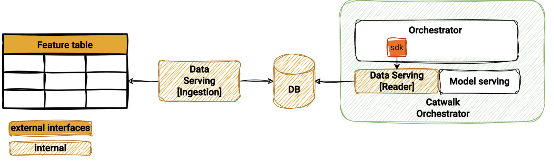
In this post, we outline how we transformed the way we serve data for our machine learning (ML) models and why we chose Amazon Aurora Postgres as the storage layer for our new feature store. At Grab, we have always been at the forefront of leveraging technology to enhance our services and provide the best possible experience for our platform users. This journey has led us to transition from a traditional approach to a more sophisticated and efficient ML feature store.
Over the years, ML at Grab has progressed from being used for specific, tactical purposes to being utilised to create long-term business value. As the complexity of our systems and ML models increased, requiring richer amounts of data over time, our platforms faced new challenges in managing more complex features such as a large number of feature keys (high-cardinality) and high-dimensional data or vectors. This evolution necessitated a shift in our data processing and management strategy. We needed a system to store and manage these complex features efficiently. In November 2023, this brought us back to the drawing board to evolve from Amphawa, our initial feature store.
We landed on the concept of feature tables: a set of data lake tables for ML features that are automatically and atomically ingested into our serving layer. While this concept is not new to the industry, as other platforms like Databricks and Tecton have evolved towards it, our approach is focused on atomicity and reproducibility. The rationale is that ensuring consistency and reliability during the serving lifecycle has become more critical, which has made it more challenging to manage within the model serving layer itself.
From feature store to data serving
A feature store is a repository that stores, serves, and manages ML features. It provides a unified platform where data scientists can access and share features, reducing redundancy and ensuring consistency across different models.
Figure 1: The high-level architecture of our centralised feature platform.
Our feature data is a key-value dataset. The key identifies a specific entity, such as a consumer ID, which is a known value in the incoming request. A composite key is supported by concatenating two or more entity identifiers. For example, (key = consumer_id + restaurant_id). The value is a binary that encodes the feature value and its type. Whenever a new value for a given entity needs to be updated, we write a new key-value pair for that entity.
New functional requirements
As our users designed and deployed increasingly complex ML solutions, new essential functional requirements were requested by our users:
Ability to retrieve the features given in the composite keys (contextual retrieval): The ML models in an upstream service might need to fetch all matching entities to form complete contextual information in order to make the recommendation. We build that context inside our ML orchestration layer before calling the model. This was previously not possible due to the design of composite keys in our initial approach.
Ability to update not just one entity atomically, but all the entities in a collection (atomic updates): This requirement concerns reducing the complexity of operations, such as rolling out new models and switching between versions of feature data. In Amphawa, newly ingested data is visible to consumer systems immediately after it’s written. As changes to the data may be ingested over a long period of time, users are responsible for ensuring the models or services don’t break while the new and old data coexist during ingestion, especially during potentially breaking changes to data. This complexity translates into quite complex code, which is hard to refactor over time. With the new approach, all feature changes will only become visible through atomic updates once the entire operation finishes successfully. This eases users’ pain of maintaining compatibility across versions.
Isolation of reading and writing capacity: The noisy-neighbor effect is one of the significant issues in our centralised feature store. Different readers could compete for read capacity. For some storage systems, write traffic could consume I/O capacity and affect reading latency. While reading capacity can be adjusted by scaling the storage, the competition between reading and writing capacity is highly dependent on the choice of storage. Hence, from the beginning, one of the top requirements of our second-generation feature store design was isolating reads from writes.
Feature table
To meet the functional requirements, we landed on the concept of a “feature table,” where users define and manage the schema and data on a per-table basis. Feature consumers can customise their tables based on their needs. Working with a table format directly makes it easier for data scientists to work with complex tabular data that needs to be retrieved in different ways depending on the context of the request. Moreover, it’s more manageable for us, on the platform side, because it’s closer to the actual format in the storage layer.
Amphawa (feature-centric)
New design (feature-table centric)
A user defines individual features and their types. Grouping into the table is storage layer is implicit.
A user defines their tables with compatibility with data-lake tools such as Spark.
The only index is on the data key.
A user defines their own indexes for their tables, based on their access pattern.
Table 1: Comparison between Amphawa and the new feature table.
Our feature tables are not just a storage solution but a critical component of our ML infrastructure. They enable us to simplify our feature management, efficiently handle the model lifecycle, and enhance our ML models’ performance. This has allowed us to provide a better experience for our platform users and dramatically improve the quality of our ML models based on our A/B testing results.
The data serving’s ingestion workflow
We designed an ingestion framework to address the atomicity requirements from the ground up.
The data ingestion process in Amphawa was meticulously crafted to ensure efficiency and reduce the pressure on the key-value store. Conversely, our priority has shifted to atomicity (all or nothing) to serve our feature tables and simplify version compatibility.
Figure 2: Ingestion workflow.
Landing feature table in the data lake: Data scientists use SQL or Python on Spark to build ML pipelines that output data lake tables. These tables and metadata for version control are stored as Parquet objects in Amazon S3.
Register collection summary: A “collection summary” consists of a group of feature tables to be served and other related metadata regarding customised individual tables. In this step, our registry will validate the table’s schema and ensure the customisations are defined correctly.
Deploy collection summary: Data scientists send another request to our registry to deploy a collection summary.
Pre-ingestion validation: The schema is validated to ensure compatibility with the target online ML models. This process ensures consistency and compatibility across feature updates.
Ingestion: The ingestion mechanism is a classic reverse ETL where the data from S3 is loaded into our Aurora Postgres tables.
Post-ingestion warm-up: To avoid cold-start latency spikes, shadow reading duplicates a part of the ongoing reading queries to the new tables for a period before the final switch.
One of the core propositions of feature tables is to offer a simplified interface for writing. Compared to writing directly to a database or providing SDKs for different processing frameworks, we provide a single, common interface for writing, independent of the actual choice of database. This allows us to evolve or even integrate feature tables with other data stores without requiring our users to modify their pipelines. We can decide how the data is represented in the database at a specific isolation level while guaranteeing total transparency for writes and reducing the complexity of read operations.
However, if a producer has access to S3 and can write in a columnar format, they can always write feature tables. This also means they can access samples from the data lake and use other tools for data validation, as well as tools for data discovery.
Do take note that a feature table can only be used for data that can be represented in tabular format and requires a minimum of one index to be present in the data. In this initial phase, we support the following data types:
Leveraging AWS Aurora for Postgres to meet our non-functional requirements
In our quest to optimise our ML infrastructure, we strategically decided to use Amazon Web Services (AWS) Aurora for PostgreSQL to meet our non-functional requirements. Aurora’s unique features and capabilities, which aligned perfectly with our operational needs, drove this decision.
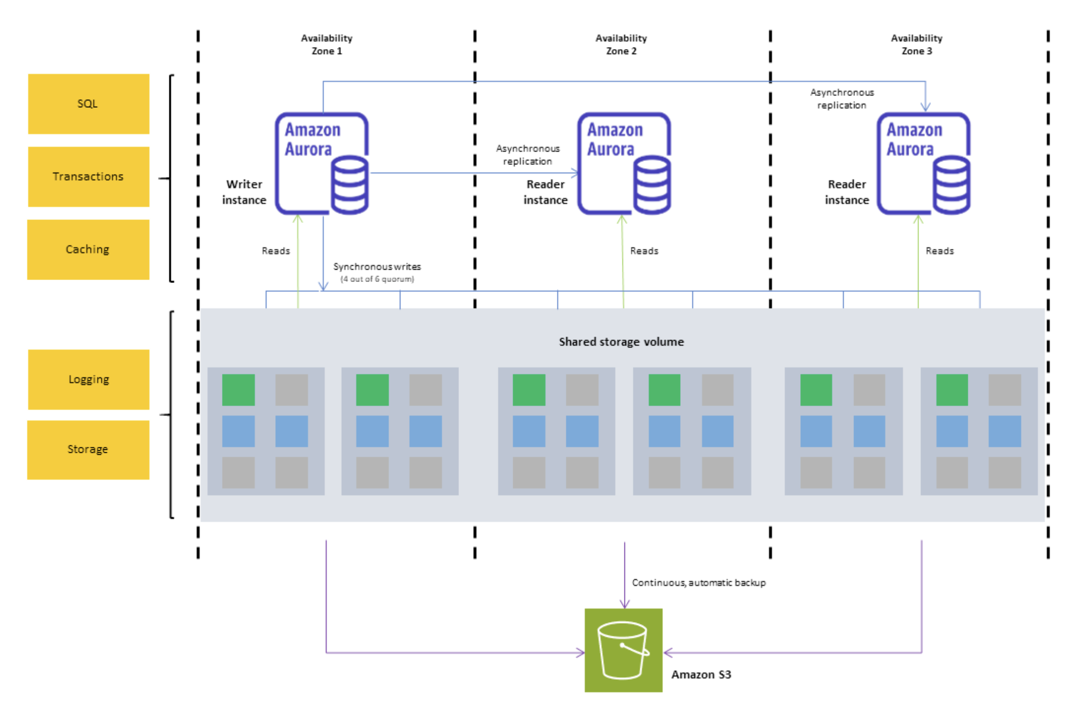
AWS Aurora is a fully managed relational database service that combines the speed and reliability of high-end commercial databases with the simplicity and cost-effectiveness of open-source databases. A key differentiator is Aurora’s distributed storage architecture.
Figure 3: AWS Aurora storage architecture.
Architecture breakdown
The cluster volume consists of copies of the data across three “Availability Zones” in a single AWS Region. Since each database instance in the cluster reads from the distributed storage, this allows for minimal replication lag and ease of scaling out read replicas to meet performance requirements as traffic patterns change.
The separation between readers and writers also allows us to scale each independently. This is a crucial feature as our traffic is predominantly read-heavy. Most of our data-writes occur once a day. Using a serverless instance class with the writer node being scaled down during idle time significantly reduces our overall operational costs.
The independent scaling of reader and writer nodes allows us to maintain high performance and availability of our feature store. During peak read times, we can scale out the reader nodes to handle the increased load, ensuring that our ML models have uninterrupted access to the features they need. Conversely, during periods of heavy data ingestion, we can scale up the writer nodes to ensure efficient data storage.
To facilitate the seamless scaling up and down of the writer node, Aurora also allows a cluster to have a mixture of Serverless and Provisioned nodes. The key difference between the two is that with Serverless, the Aurora service manages the capacity of a single node and adjusts accordingly as the load increases and decreases. In our context, we’re using Serverless for our writer node to quickly scale up when heavy data ingestion starts and scale down automatically once the ingestion is done. We then use Provisioned nodes for the reader nodes since read traffic is more consistent.
In addition to cost and performance benefits, AWS Aurora simplifies our database management tasks. As a fully managed service, Aurora takes care of time-consuming database administration tasks such as hardware provisioning, software patching, setup, configuration, or backups, allowing our team to focus on optimising our ML models.
Accessing the data through our SDK
With the goal of providing a high-performing and highly available data serving SDK design, we’ve moved on from the centralised API design of Amphawa to a decentralised access architecture in Data Serving. Each data serving deployment is a self-contained system with a cluster and feature catalogue stored within the cluster as additional metadata tables. This minimises dependency, which improves the availability of the system.
The data serving SDK is designed to be a thin wrapper around the database driver to optimise performance. The SDK contains only a set of utility functions that load user configuration from the Catwalk platform and a query builder to translate user queries to SQL. No additional data validation is performed in the query code path, as all validation is done during feature table generation and ingestion. Therefore, the database handles most of the heavy lifting.
Decentralised deployments: A strategic shift in our infrastructure
We also investigated the difference between centralised and decentralised deployments. We have been exploring these options in the context of our ML feature store, specifically with our Amphawa service and Catwalk orchestrators.
Our original feature store was deployed as a standalone service where different model-serving applications can connect to it. On the other hand, a decentralised deployment is integrated within a model-serving orchestrator, and a specific orchestrator is bound to a set of pods.
After extensive discussions and evaluations, we concluded that a decentralised deployment for data serving would better align with our operational needs and objectives. Below is the list of factors we compared that led us to this decision:
Version control: Centralised deployments simplify version control but risk accumulating technical debt due to backward compatibility requirements. Decentralised deployments, while needing robust tracking, offer more flexibility.
Deployment strategies: Decentralised deployments enabled seamless use of Blue-green and Rolling Deployment strategies. They allow multiple versions to coexist and easy rollbacks, reducing client mismatch issues.
Noisy neighbour problem: Centralised deployments struggle with the noisy neighbour issue, which requires complex rate limiting. Decentralised setups mitigate this problem by isolating services.
Caching efficiency: Centralised deployments often suffer low cache hits, whereas decentralised deployments improve caching efficiency by better fitting data into the cache.
Conclusion
In conclusion, leveraging AWS Aurora for Postgres has enabled us to create a robust, scalable, and cost-effective feature store that supports our complex ML infrastructure. This is a testament to our commitment to using cutting-edge technology to enhance our services and provide the best possible experience for our users. Our shift towards decentralised deployments represents our dedication to optimising our infrastructure to support our ML models effectively. By aligning our deployment strategy with our operational needs, we aim to enhance the performance of our services and provide the best possible experience for our users.
Join us
Grab is a leading superapp in Southeast Asia, operating across the deliveries, mobility and digital financial services sectors. Serving over 800 cities in eight Southeast Asian countries, Grab enables millions of people everyday to order food or groceries, send packages, hail a ride or taxi, pay for online purchases or access services such as lending and insurance, all through a single app. Grab was founded in 2012 with the mission to drive Southeast Asia forward by creating economic empowerment for everyone. Grab strives to serve a triple bottom line – we aim to simultaneously deliver financial performance for our shareholders and have a positive social impact, which includes economic empowerment for millions of people in the region, while mitigating our environmental footprint.
Powered by technology and driven by heart, our mission is to drive Southeast Asia forward by creating economic empowerment for everyone. If this mission speaks to you, join our team today!
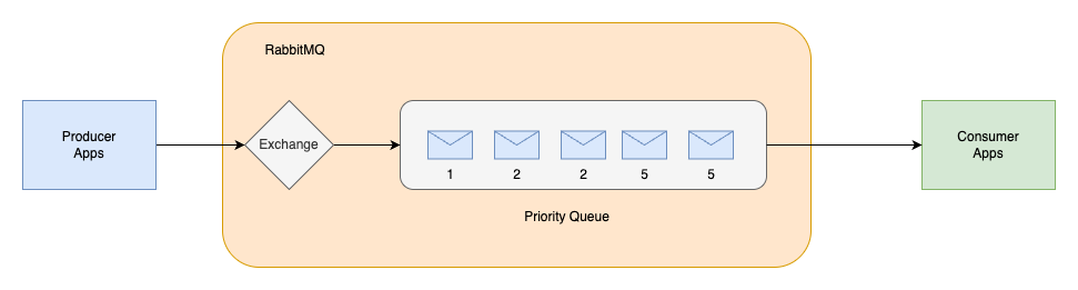
Quorum queues are now available on Amazon MQ for RabbitMQ from version 3.13. Quorum queues are a replicated First-In, First-Out (FIFO) queue type that uses the Raft consensus algorithm to maintain data consistency. Quorum queues on RabbitMQ version 3.13 lack one key feature compared to classic queues: message prioritization. However, RabbitMQ version 4.0 introduced support for message priority, which behaves differently than classic queue message priorities. Migrating applications from classic queues with message priority to quorum queues on Amazon MQ for RabbitMQ presents challenges for customers. This post describes the different approaches to implementing message prioritization in quorum queues in Amazon MQ for RabbitMQ.
Amazon MQ is a managed message broker service for Apache ActiveMQ and RabbitMQ that simplifies setting up and operating message brokers on AWS.
Why message prioritization matters
Modern messaging systems require handling messages differently, depending on the business priority. Some messages are more time-sensitive or critical than others and prioritizing them can enhance the efficiency and responsiveness of applications. Message prioritization allows certain messages to be processed before others, aligning with business priorities and helping to ensure that high-value or time-critical messages receive the attention they need.
Message prioritization addresses critical business challenges across multiple industries. In insurance companies, it can expedite urgent claim processing by prioritizing high-priority messages over routine policy updates, reducing settlement times. Automotive manufacturers can make sure that critical production line alerts and safety notifications take precedence over standard telemetry data, preventing costly downtime. Energy utilities can prioritize real-time grid stability alerts and outage notifications, enabling faster responses to potential blackouts. By implementing message priority, industries can direct immediate attention to time-sensitive operations while efficiently managing routine processes within existing infrastructure. By using this approach to transform their communication strategies, organizations can respond more quickly and effectively to critical events.
Classic queues compared to quorum queues message prioritization
In this section, explore the fundamental differences between classic queues and quorum queues when it comes to message prioritization capabilities. Examine how each queue type handles message priority, the built-in features available, and key considerations.
Message prioritization with classic queues
In classic queues, RabbitMQ supports message priorities ranging from 1 to 255, with 1 being the lowest priority and 255 being the highest. However, it’s generally recommended to use a smaller range (for example, 1–5) for better performance, because RabbitMQ needs to maintain an internal sub-queue for each priority from 1 up to the maximum value configured for a given queue. A wider priority range adds more CPU and memory cost, which can impact broker performance.
Priority queue behavior in classic queues:
Classic queues require x-max-priority argument to define the maximum number of priorities for a given queue
A procedure sends a message with a priority property value
Consumers don’t need special configuration to handle priorities
Messages with higher priority are delivered before messages with lower priority
Within the same priority level, messages are delivered in FIFO order
Messages without a priority property are treated as if their priority is lowest
Messages with a priority that is higher than the queue’s maximum are treated as if they were published with the maximum priority
Example Python code for classic queue implementation with message priority:
#!/usr/bin/env python
import pika
import ssl
# Set up SSL context for secure connection
context = ssl.SSLContext(ssl.PROTOCOL_TLSv1_2)
# Define credentials
credentials = pika.PlainCredentials('username', 'password') # Replace with actual credentials
# Set up connection parameters for Amazon MQ RabbitMQ broker
connection_parameters = pika.ConnectionParameters(
    host='b-example.mq.us-west-2.on.aws', # Replace with actual broker endpoint
    port=5671,
    credentials=credentials,
    ssl_options=pika.SSLOptions(context)
)
# Establish connection and create a channel
connection = pika.BlockingConnection(connection_parameters)
channel = connection.channel()
# Declare a direct exchange
# - direct exchanges route messages based on routing key
channel.exchange_declare(
    exchange='priority_exchange',
    exchange_type='direct',
)
# Declare a priority queue
# - x-max-priority=5 sets maximum priority level (0-5)
# - x-queue-type=classic specifies classic queue implementation
channel.queue_declare(
    queue='classic_priority_queue',
    arguments={
        'x-max-priority': 5,
        'x-queue-type': "classic"
    }
)
# Bind queue to exchange with routing key
# - This connects the queue to the exchange
# - Messages sent to the exchange with matching routing key will be routed to this queue
channel.queue_bind(
    queue='classic_priority_queue',
    exchange='priority_exchange',
    routing_key='priority_queue'
)
# Publish messages with different priorities
# Low priority message (priority=1)
channel.basic_publish(
    exchange='priority_exchange',
    routing_key='priority_queue',
    body='Low priority message',
    properties=pika.BasicProperties(priority=1)
)
print(" [x] Sent 'Low priority message'")
# Medium priority message (priority=2)
channel.basic_publish(
    exchange='priority_exchange',
    routing_key='priority_queue',
    body='Medium priority message',
    properties=pika.BasicProperties(priority=2)
)
print(" [x] Sent 'Medium priority message'")
# High priority message (priority=5)
channel.basic_publish(
    exchange='priority_exchange',
    routing_key='priority_queue',
    body='High priority message',
    properties=pika.BasicProperties(priority=5)
)
print(" [x] Sent 'High priority message'")
# Close the connection
connection.close()
The preceding code demonstrates message prioritization in RabbitMQ using a classic queue with built-in priority handling. The implementation connects to a RabbitMQ broker using the Python Pika library and declares a direct exchange, a classic queue with a maximum priority level of 5. Messages are then published to this single queue with explicitly assigned priority values (1 for low, 2 for medium, and 5 for high priority). When consumers fetch messages from this queue, RabbitMQ will deliver higher priority messages first.
Message prioritization with quorum queues
Unlike classic queues, quorum queues in Rabbit MQ 3.13 don’t support message prioritization natively. However, there are effective patterns that you can implement to achieve message priority with Quorum queues.
Using separate queues for different priorities
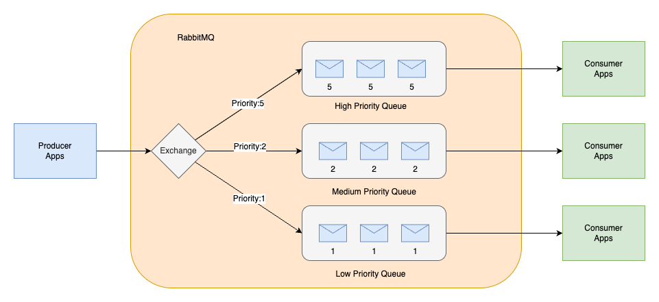
A straightforward method is to create multiple quorum queues, each dedicated to different priority levels. For example, you might have a high-priority queue and a low-priority queue. Using RabbitMQ exchange and binding key route messages to the appropriate queues based on their priority, allowing the system to process high-priority messages more promptly, as shown in the following figure.
Example to implement priority handling using separate quorum queues:
#!/usr/bin/env python
import pika
import ssl
# Set up SSL context for secure connection
context = ssl.SSLContext(ssl.PROTOCOL_TLSv1_2)
# Define credentials
credentials = pika.PlainCredentials('username', 'password') #Replace with actual credentials
# Set up connection parameters for Amazon MQ RabbitMQ broker
connection_parameters = pika.ConnectionParameters(
    host='b-example.mq.us-west-2.on.aws',
    port=5671,
    credentials=credentials,
    ssl_options=pika.SSLOptions(context)
)
# Establish connection and create a channel
connection = pika.BlockingConnection(connection_parameters)
channel = connection.channel()
# Declare a direct exchange
# - Direct exchanges route messages based on routing key
channel.exchange_declare(
    exchange='priority_exchange_qq',
    exchange_type='direct'
)
# Create separate quorum queues for different priority levels
# Low priority queue
channel.queue_declare(
    queue='low_priority_queue',
    durable=True,
    arguments={
        'x-queue-type': "quorum"
    }
)
# Bind the low priority queue to the exchange with a specific routing key
# - This creates a rule that messages sent to 'priority_exchange' with routing_key='low_priority_1'
# - will be routed to the 'low_priority_queue'
channel.queue_bind(
    queue='low_priority_queue',
    exchange='priority_exchange_qq',
    routing_key='low_priority_1'
)
# Medium priority queue
channel.queue_declare(
    queue='medium_priority_queue',
    durable=True,
    arguments={
        'x-queue-type': "quorum"
    }
)
# Bind the medium priority queue to the exchange with a specific routing key
# - Messages with routing_key='medium_priority_2' will be directed to the 'medium_priority_queue'
channel.queue_bind(
    queue='medium_priority_queue',
    exchange='priority_exchange_qq',
    routing_key='medium_priority_2'
)
# High priority queue
channel.queue_declare(
    queue='high_priority_queue',
    durable=True,
    arguments={
        'x-queue-type': "quorum"
    }
)
# Bind the high priority queue to the exchange with a specific routing key
# - Messages with routing_key='high_priority_2' will be directed to the 'high_priority_queue'
channel.queue_bind(
    queue='high_priority_queue',
    exchange='priority_exchange_qq',
    routing_key='high_priority_5'
)
# Publish messages to different priority queues
print(" [x] Publishing messages to different priority queues")
# Low priority message
channel.basic_publish(
    exchange='priority_exchange_qq',
    routing_key='low_priority_1',
    body='Low priority message'
)
print(" [x] Sent 'Low priority message'")
# Medium priority message
channel.basic_publish(
    exchange='priority_exchange_qq',
    routing_key='medium_priority_2',
    body='Medium priority message'
)
print(" [x] Sent 'Medium priority message'")
# High priority message
channel.basic_publish(
    exchange='priority_exchange_qq',
    routing_key='high_priority_5',
    body='High priority message'
)
print(" [x] Sent 'High priority message'")
# Close the connection
connection.close()
print(" [x] Connection closed")
The preceding code demonstrates a message prioritization approach in RabbitMQ using separate quorum queues for different priority levels (low, medium, and high). The implementation uses the Python Pika library to connect to a RabbitMQ server, a direct exchange and three separate quorum queues for different priority levels, and publish messages to different routing keys with different priority.
Custom priority logic on consumers
Implement custom logic within your application to handle messages based on their priority. For example, you can use headers or metadata to determine the priority of a message and then use this information to route messages to different queues or handle them in a specific order.
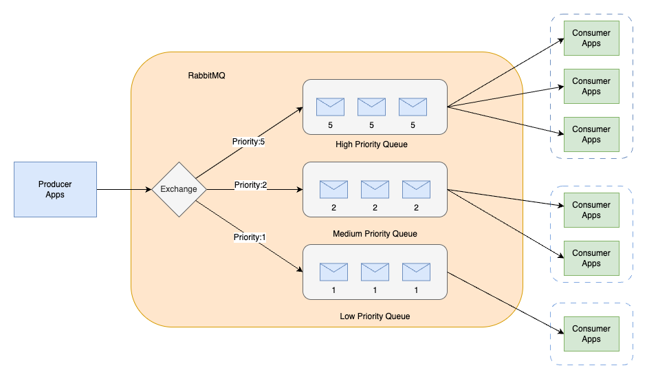
Higher priority queues should use more consumers or consumers with higher resources allocated to process messages more quickly than lower priority queues. Use the basic.qos (prefetch) method in manual acknowledgement mode on your consumers to limit the number of messages that can be out for delivery at any time and allow messages to be prioritized. basic.qos is a value a consumer sets when connecting to a queue. It indicates how many messages the consumer can handle at one time. This method is shown in the following figure.
Note: This solution implements message priority on a best-effort basis. There is a possibility that low and medium priority messages may be processed before high priority messages.
Conclusion
Message prioritization in RabbitMQ brokers on Amazon MQ has different considerations for classic and quorum queues. Using quorum queues requires a thoughtful approach because of the lack of native support for message proritization in RabbitMQ. By employing separate queues and custom logic, you can achieve effective prioritization while maintaining the high availability and consistency that quorum queues offer. Embrace these strategies to optimize your messaging infrastructure, enhance application responsiveness, and make sure that critical messages are processed in a timely manner.
We recommend that you adopt quorum queues as the preferred replicated queue type on RabbitMQ 3.13 brokers. For more details, see Amazon MQ documentation. For more information, see quorum queues.
We’re excited to announce the release of our latest whitepaper, AICPA SOC 2 Compliance Guide on AWS, which provides in-depth guidance on implementing and maintaining SOC 2-aligned controls using AWS services.
Building and operating cloud-native services in alignment with the AICPA’s Trust Services Criteria requires thoughtful planning and robust implementation. This new whitepaper helps cloud architects, security and compliance teams, and DevOps professionals design environments that meet SOC 2 requirements while leveraging AWS’s shared responsibility model.
What’s inside the whitepaper:
Overview of the SOC 2 framework—including Common Criteria (CC 1–CC 9) and category-specific criteria (Security, Availability, Processing Integrity, Confidentiality, Privacy)
Mapping of each Trust Services Criterion to AWS services and constructs
Guidance on implementing complementary user entity controls (CUECs)
Strategies for evidence collection, documentation, and audit procedures
Risk and governance for executives
Best practices for automating compliance and preparing for SOC 2 readiness assessments
Organizations running Apache Spark workloads, whether on Amazon EMR, AWS Glue, Amazon Elastic Kubernetes Service (Amazon EKS), or self-managed clusters, invest countless engineering hours in performance troubleshooting and optimization. When a critical extract, transform, and load (ETL) pipeline fails or runs slower than expected, engineers end up spending hours navigating through multiple interfaces such as logs or Spark UI, correlating metrics across different systems and manually analyzing execution patterns to identify root causes. Although Spark History Server provides detailed telemetry data, including job execution timelines, stage-level metrics, and resource consumption patterns, accessing and interpreting this wealth of information requires deep expertise in Spark internals and navigating through multiple interconnected web interface tabs.
Today, we’re announcing the open source release of Spark History Server MCP, a specialized Model Context Protocol (MCP) server that transforms this workflow by enabling AI assistants to access and analyze your existing Spark History Server data through natural language interactions. This project, developed collaboratively by AWS open source and Amazon SageMaker Data Processing, turns complex debugging sessions into conversational interactions that deliver faster, more accurate insights without requiring changes to your current Spark infrastructure. You can use this MCP server with your self-managed or AWS managed Spark History Servers to analyze Spark applications running in the cloud or on-premises deployments.
Understanding Spark observability challenge
Apache Spark has become the standard for large-scale data processing, powering critical ETL pipelines, real-time analytics, and machine learning (ML) workloads across thousands of organizations. Building and maintaining Spark applications is, however, still an iterative process, where developers spend significant time testing, optimizing, and troubleshooting their code. Spark application developers focused on data engineering and data integration use cases often encounter significant operational challenges due to a few different reasons:
Complex connectivity and configuration optionsto a variety of resources with Spark – Although this makes it a popular data processing platform, it often makes it challenging to find the root cause of inefficiencies or failures when Spark configurations aren’t optimally or correctly configured.
Spark’s in-memory processing model and distributed partitioning of datasetsacross its workers – Although good for parallelism, this often makes it difficult for users to identify inefficiencies. This results in slow application execution or root cause of failures caused by resource exhaustion issues such as out of memory and disk exceptions.
Lazy evaluation of Spark transformations – Although lazy evaluation optimizes performance, it makes it challenging to accurately and quickly identify the application code and logic that caused the failure from the distributed logs and metrics emitted from different executors.
Spark History Server
Spark History Server provides a centralized web interface for monitoring completed Spark applications, serving comprehensive telemetry data including job execution timelines, stage-level metrics, task distribution, executor resource consumption, and SQL query execution plans. Although Spark History Server assists developers for performance debugging, code optimization, and capacity planning, it still has challenges:
Time-intensive manual workflows – Engineers spend hours navigating through the Spark History Server UI, switching between multiple tabs to correlate metrics across jobs, stages, and executors. Engineers must constantly switch between the Spark UI, cluster monitoring tools, code repositories, and documentation to piece together a complete picture of application performance, which often takes days.
Expertise bottlenecks – Effective Spark debugging requires deep understanding of execution plans, memory management, and shuffle operations. This specialized knowledge creates dependencies on senior engineers and limits team productivity.
Reactive problem-solving – Teams typically discover performance issues only after they impact production systems. Manual monitoring approaches don’t scale to proactively identify degradation patterns across hundreds of daily Spark jobs.
How MCP transforms Spark observability
The Model Context Protocol provides a standardized interface for AI agents to access domain-specific data sources. Unlike general-purpose AI assistants operating with limited context, MCP-enabled agents can access technical information about specific systems and provide insights based on actual operational data rather than generic recommendations.With the help of Spark History Server accessible through MCP, instead of manually gathering performance metrics from multiple sources and correlating them to understand application behavior, engineers can engage with AI agents that have direct access to all Spark execution data. These agents can analyze execution patterns, identify performance bottlenecks, and provide optimization recommendations based on actual job characteristics rather than general best practices.
Introduction to Spark History Server MCP
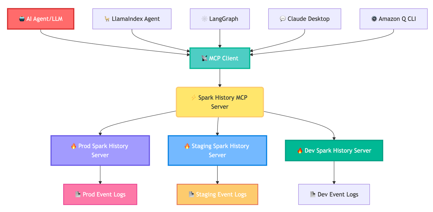
The Spark History Server MCP is a specialized bridge between AI agents and your existing Spark History Server infrastructure. It connects to one or more Spark History Server instances and exposes their data through standardized tools that AI agents can use to retrieve application metrics, job execution details, and performance data.
The Spark History Server MCP directly addresses these operational challenges by enabling AI agents to access Spark performance data programmatically. This transforms the debugging experience from manual UI navigation to conversational analysis. Instead of hours in the UI, ask, “Why did job spark-abcd fail?” and receive root cause analysis of the failure. This allows users to use AI agents for expert-level performance analysis and optimization recommendations, without requiring deep Spark expertise.
The MCP server provides comprehensive access to Spark telemetry across multiple granularity levels. Application-level tools retrieve execution summaries, resource utilization patterns, and success rates across job runs. Job and stage analysis tools provide execution timelines, stage dependencies, and task distribution patterns for identifying critical path bottlenecks. Task-level tools expose executor resource consumption patterns and individual operation timings for detailed optimization analysis. SQL-specific tools provide query execution plans, join strategies, and shuffle operation details for analytical workload optimization. You can review the complete set of tools available in the MCP server in the project README.
How to use the MCP server
The MCP is an open standard that enables secure connections between AI applications and data sources. This MCP server implementation supports both Streamable HTTP and STDIO protocols for maximum flexibility.
The MCP server runs as a local service within your infrastructure either on Amazon Elastic Compute Cloud (Amazon EC2) or Amazon EKS, connecting directly to your Spark History Server instances. You maintain complete control over data access, authentication, security, and scalability.
All the tools are available with streamable HTTP and STDIO protocol:
Streamable HTTP – Full advanced tools for LlamaIndex, LangGraph, and programmatic integrations
For deployment, it supports multiple Spark History Server instances and provides deployments with AWS Glue, Amazon EMR, and Kubernetes.
Quick local setup
To set up Spark History MCP server locally, execute the following commands in your terminal:
git clone
cd spark-history-server-mcp

# Install Task (if not already installed)
brew install go-task # macOS, see  for others

# Setup and start testing
task install            # Install dependencies
task start-spark-bg     # Start Spark History Server with sample data
task start-mcp-bg       # Start MCP Server
task start-inspector-bg # Start MCP Inspector

# Opens  for interactive testing
# When done, run task stop-all
For comprehensive configuration examples and integration guides, refer to the project README.
Integration with AWS managed services
The Spark History Server MCP integrates seamlessly with AWS managed services, offering enhanced debugging capabilities for Amazon EMR and AWS Glue workloads. This integration adapts to various Spark History Server deployments available across these AWS managed services while providing a consistent, conversational debugging experience:
AWS Glue – Users can use the Spark History Server MCP integration with self-managed Spark History Server on an EC2 instance or launch locally using Docker container. Setting up the integration is straightforward. Follow the step-by-step instructions in the README to configure the MCP server with your preferred Spark History Server deployment. Using this integration, AWS Glue users can analyze AWS Glue ETL job performance regardless of their Spark History Server deployment approach.
Amazon EMR – Integration with Amazon EMR uses the service-managed Persistent UI feature for EMR on Amazon EC2. The MCP server requires only an EMR cluster Amazon Resource Name (ARN) to discover the available Persistent UI on the EMR cluster or automatically configure a new one for cases its missing with token-based authentication. This eliminates the need for manually configuring Spark History Server setup while providing secure access to detailed execution data from EMR Spark applications. Using this integration, data engineers can ask questions about their Spark workloads, such as “Can you get job bottle neck for spark-<emr-applicationId>? ” The MCP responds with detailed analysis of execution patterns, resource utilization differences, and targeted optimization recommendations, so teams can fine-tune their Spark applications for optimal performance across AWS services.
For comprehensive configuration examples and integration details, refer to the AWS Integration Guides.
Looking ahead: The future of AI-assisted Spark optimization
This open-source release establishes the foundation for enhanced AI-powered Spark capabilities. This project establishes the foundation for deeper integration with AWS Glue and Amazon EMR to simplify the debugging and optimization experience for customers using these Spark environments. The Spark History Server MCP is open source under the Apache 2.0 license. We welcome contributions including new tool extensions, integrations, documentation improvements, and deployment experiences.
Get started today
Transform your Spark monitoring and optimization workflow today by providing AI agents with intelligent access to your performance data.
Review the comprehensive README for setup and integration instructions
Join discussions and submit issues for enhancements
Contribute new features and deployment patterns
Acknowledgment: A special thanks to everyone who contributed to the development and open-sourcing of the Apache Spark history server MCP: Vaibhav Naik, Akira Ajisaka, Rich Bowen, Savio Dsouza.
About the authors
Manabu McCloskey is a Solutions Architect at Amazon Web Services. He focuses on contributing to open source application delivery tooling and works with AWS strategic customers to design and implement enterprise solutions using AWS resources and open source technologies. His interests include Kubernetes, GitOps, Serverless, and Souls Series.
Vara Bonthu is a Principal Open Source Specialist SA leading Data on EKS and AI on EKS at AWS, driving open source initiatives and helping AWS customers to diverse organizations. He specializes in open source technologies, data analytics, AI/ML, and Kubernetes, with extensive experience in development, DevOps, and architecture. Vara focuses on building highly scalable data and AI/ML solutions on Kubernetes, enabling customers to maximize cutting-edge technology for their data-driven initiatives
Andrew Kim is a Software Development Engineer at AWS Glue, with a deep passion for distributed systems architecture and AI-driven solutions, specializing in intelligent data integration workflows and cutting-edge feature development on Apache Spark. Andrew focuses on re-inventing and simplifying solutions to complex technical problems, and he enjoys creating web apps and producing music in his free time.
Shubham Mehta is a Senior Product Manager at AWS Analytics. He leads generative AI feature development across services such as AWS Glue, Amazon EMR, and Amazon MWAA, using AI/ML to simplify and enhance the experience of data practitioners building data applications on AWS.
Kartik Panjabi is a Software Development Manager on the AWS Glue team. His team builds generative AI features for the Data Integration and distributed system for data integration.
Mohit Saxena is a Senior Software Development Manager on the AWS Data Processing Team (AWS Glue and Amazon EMR). His team focuses on building distributed systems to enable customers with new AI/ML-driven capabilities to efficiently transform petabytes of data across data lakes on Amazon S3, databases and data warehouses on the cloud.
We know that there are plenty of users out there who will have been
affected by the problem, and found themselves unable to communicate as
a result. We very much share your frustration, and we’d like to
apologise for the disruption to service.
With that said, we’re glad that we were able to get to the bottom
of most of the problem, and get the lost data restored within a
relatively short time. If nothing else, hopefully this blog post will
be of use to future generations faced with Postgres index
corruption!
Providing security updates for a Linux distribution, such as
Debian, involves a lot of work behind the scenes—and requires
much more than simply shipping the latest code. On July 15, at DebConf25 in Brest, France,
Samuel Henrique walked through the process of providing security
updates to users; he discussed how Debian learns about security
vulnerabilities, decides on the best response, and the process of
sending out updates to keep its users safe. He also provided guidance
on how others could get involved.
The Home Assistant project has published
an update on improvements in its Android app, and plans for upcoming releases:
In our latest update of the Android app 2025.7.1, we’ve added a
couple of useful features. Including a new basic invite flow, which
will be shared between Android and iOS, adding a good layer of
consistency between our most-used companion apps. The idea is to make
it much more seamless to add new users or set up new devices (no need
to type the URL in your Android Automotive device!).
We’ve also made My
Links work better. If you’re unfamiliar with My Links, they’re
those cool links (that anyone can
make) that bring you right to an integration, blueprint, add-on,
or settings page. They have always worked great on desktop, but up
until recently, they were a bit clunky to use on mobile. Now you can
get to the link’s destination with a single click.
The Cloudflare Business Intelligence team manages a petabyte-scale data lake and ingests thousands of tables every day from many different sources. These include internal databases such as Postgres and ClickHouse, as well as external SaaS applications such as Salesforce. These tasks are often complex and tables may have hundreds of millions or billions of rows of new data each day. They are also business-critical for product decisions, growth plannings, and internal monitoring. In total, about 141 billion rows are ingested every day.
As Cloudflare has grown, the data has become ever larger and more complex. Our existing Extract Load Transform (ELT) solution could no longer meet our technical and business requirements. After evaluating other common ELT solutions, we concluded that their performance generally did not surpass our current system, either.
It became clear that we needed to build our own framework to cope with our unique requirements — and so Jetflow was born.
What we achieved
Over 100x efficiency improvement in GB-s:
Our longest running job with 19 billion rows was taking 48 hours using 300 GB of memory, and now completes in 5.5 hours using 4 GB of memory
We estimate that ingestion of 50 TB from Postgres via Jetflow could cost under $100 based on rates published by commercial cloud providers
>10x performance improvement:
Our largest dataset was ingesting 60-80,000 rows per second, this is now 2-5 million rows per second per database connection.
In addition, these numbers scale well with multiple database connections for some databases.
Extensibility:
The modular design makes it easy to extend and test. Today Jetflow works with ClickHouse, Postgres, Kafka, many different SaaS APIs, Google BigQuery and many others. It has continued to work well and remain flexible with the addition of new use cases.
How did we do this?
Requirements
The first step to designing our new framework had to be a clear understanding of the problems we were aiming to solve, with clear requirements to stop us creating new ones.
Performant & efficient
We needed to be able to move more data in less time as some ingestion jobs were taking ~24 hours, and our data will only grow. The data should be ingested in a streaming fashion and use less memory and compute resources than our existing solution.
Backwards compatible
Given the daily ingestion of thousands of tables, the chosen solution needed to allow for the migration of individual tables as needed. Due to our usage of Spark downstream and Spark’s limitations in merging desperate Parquet schemas, the chosen solution had to offer the flexibility to generate the precise schemas needed for each case to match legacy.
We also required seamless integration with our custom metadata system, used for dependency checks and job status information.
Ease of use
We want a configuration file that can be version-controlled, without introducing bottlenecks on repositories with many concurrent changes.
To increase accessibility for different roles within the team, another requirement was no-code (or configuration as code) in the vast majority of cases. Users should not have to worry about availability or translation of data types between source and target systems, or writing new code for each new ingestion. The configuration needed should also be minimal — for example, data schema should be inferred from the source system and not need to be supplied by the user.
Customizable
Striking a balance with the no-code requirement above, although we want a low bar of entry we also want to have the option to tune and override options if desired, with a flexible and optional configuration layer. For example, writing Parquet files is often more expensive than reading from the database, so we want to be able to allocate more resources and concurrency as needed.
Additionally, we wanted to allow for control over where the work is executed, with the ability to spin up concurrent workers in different threads, different containers, or on different machines. The execution of workers and communication of data was abstracted away with an interface, and different implementations can be written and injected, controlled via the job configuration.
Testable
We wanted a solution capable of running locally in a containerized environment, which would allow us to write tests for every stage of the pipeline. With “black box” solutions, testing often means validating the output after making a change, which is a slow feedback loop, risks not testing all edge cases as there isn’t good visibility of all code paths internally, and makes debugging issues painful.
Designing a flexible framework
To build a truly flexible framework, we broke the pipeline down into distinct stages, and then create a config layer to define the composition of the pipeline from these stages, and any configuration overrides. Every pipeline configuration that makes sense logically should execute correctly, and users should not be able to create pipeline configs that do not work.
Pipeline configuration
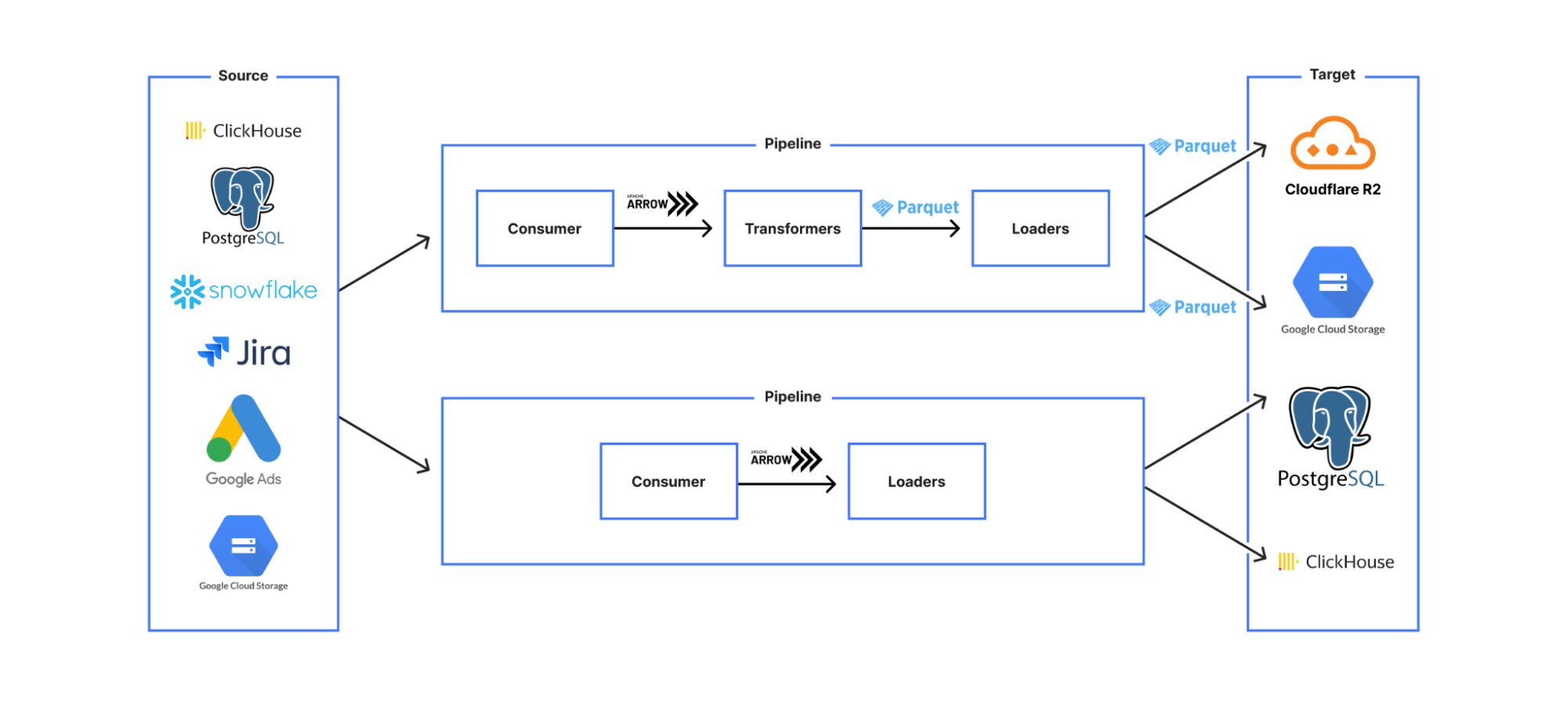
This led us to a design where we created stages which were classified according to the meaningfully different categories of:
Consumers
Transformers
Loaders
The pipeline was constructed via a YAML file that required a consumer, zero or more transformers, and at least one loader. Consumers create a data stream (via reading from the source system), Transformers (e.g. data transformations, validations) take a data stream input and output a data stream conforming to the same API so that they can be chained, and Loaders have the same data streaming interface, but are the stages with persistent effects — i.e. stages where data is saved to an external system.
This modular design means that each stage is independently testable, with shared behaviour (such as error handling and concurrency) inherited from shared base stages, significantly decreasing development time for new use cases and increasing confidence in code correctness.
Data divisions
Next, we designed a breakdown for the data that would allow the pipeline to be idempotent both on whole pipeline re-run and also on internal retry of any data partition due to transient error. We decided on a design that let us parallelize processing, while maintaining meaningful data divisions that allowed the pipeline to perform cleanups of data where required for a retry.
RunInstance: the least granular division, corresponding to a business unit for a single run of the pipeline (e.g. one month/day/hour of data).
Partition: a division of the RunInstance that allows each row to be allocated to a partition in a way that is deterministic and self-evident from the row data without external state, and is therefore idempotent on retry. (e.g. an accountId range, a 10-minute interval)
Batch: a division of the partition data that is non-deterministic and used only to break the data down into smaller chunks for streaming/parallel processing for faster processing with fewer resources. (e.g. 10k rows, 50 MB)
The options that the user configures in the consumer stage YAML both construct the query that is used to retrieve the data from the source system, and also encode the semantic meaning of this data division in a system agnostic way, so that later stages understand what this data represents — e.g. this partition contains the data for all accounts IDs 0-500. This means that we can do targeted data cleanup and avoid, for example, duplicate data entries if a single data partition is retried due to error.
Framework implementation
Standard internal state for stage compatibility
Our most common use case is something like read from a database, convert to Parquet format, and then save to object storage, with each of these steps being a separate stage. As more use cases were onboarded to Jetflow, we had to make sure that if someone wrote a new stage it would be compatible with the other stages. We don’t want to create a situation where new code needs to be written for every output format and target system, or you end up with a custom pipeline for every different use case.
The way we have solved this problem is by having our stage extractor class only allow output data in a single format. This means as long as any downstream stages support this format as in the input and output format they would be compatible with the rest of the pipeline. This seems obvious in retrospect, but internally was a painful learning experience, as we originally created a custom type system and struggled with stage interoperability.
For this internal format, we chose to use Arrow, an in-memory columnar data format. The key benefits of this format for us are:
Arrow ecosystem: Many data projects now support Arrow as an output format. This means when we write extractor stages for new data sources, it is often trivial to produce Arrow output.
No serialisation overhead: This makes it easy to move Arrow data between machines and even programming languages with minimum overhead. Jetflow was designed from the start to have the flexibility to be able to run in a wide range of systems via a job controller interface, so this efficiency in data transmission means there’s minimal compromise on performance when creating distributed implementations.
Reserve memory in large fixed-size batches to avoid memory allocations: As Go is a garbage collected (GC) language and GC cycle times are affected mostly by the number of objects rather than the sizes of those objects, fewer heap objects reduces CPU time spent garbage collecting significantly, even if the total size is the same. As the number of objects to scan, and possibly collect, during a GC cycle increases with the number of allocations, if we have 8192 rows with 10 columns each, Arrow would only require us to do 10 allocations versus the 8192 allocations of most drivers that allocate on a row by row basis, meaning fewer objects and lower GC cycle times with Arrow.
Converting rows to columns
Another important performance optimization was reducing the number of conversion steps that happen when reading and processing data. Most data ingestion frameworks internally represent data as rows. In our case, we are mostly writing data in Parquet format, which is column based. When reading data from column-based sources (e.g. ClickHouse, where most drivers receive RowBinary format), converting into row-based memory representations for the specific language implementation is inefficient. This is then converted again from rows to columns to write Parquet files. These conversions result in a significant performance impact.
Jetflow instead reads data from column-based sources in columnar formats (e.g. for ClickHouse-native Block format) and then copies this data into Arrow column format. Parquet files are then written directly from Arrow columns. The simplification of this process improves performance.
Writing each pipelines stage
Case study: ClickHouse
When testing an initial version of Jetflow, we discoveredthat due to the architecture of ClickHouse, using additional connections would not be of any benefit, since ClickHouse was reading faster than we were receiving data. It should then be possible, with a more optimized database driver, to take better advantage of that single connection to read a much larger number of rows per second, without needing additional connections.
Initially, a custom database driver was written for ClickHouse, but we ended up switching to the excellent ch-go low level library, which directly reads Blocks from ClickHouse in a columnar format. This had a dramatic effect on performance in comparison to the standard Go driver. Combined with the framework optimisations above, we now ingest millions of rows per second with a single ClickHouse connection.
A valuable lesson learned is that as with any software, tradeoffs are often made for the sake of convenience or a common use case that may not match your own. Most database drivers tend not to be optimized for reading large batches of rows, and have high per-row overhead.
Case study: Postgres
For Postgres, we use the excellent jackc/pgx driver, but instead of using the database/sql Scan interface, we directly receive the raw bytes for each row and use the jackc/pgx internal scan functions for each Postgres OID (Object Identifier) type.
The database/sql Scan interface in Go uses reflection to understand the type passed to the function and then also uses reflection to set each field with the column value received from Postgres. In typical scenarios, this is fast enough and easy to use, but falls short for our use cases in terms of performance. The jackc/pgx driver reuses the row bytes produced each time the next Postgres row is requested, resulting in zero allocations per row. This allows us to write high-performance, low-allocation code within Jetflow. With this design, we are able to achieve nearly 600,000 rows per second per Postgres connection for most tables, with very low memory usage.
Conclusion
As of early July 2025, the team ingests 77 billion records per day via Jetflow. The remaining jobs are in the process of being migrated to Jetflow, which will bring the total daily ingestion to 141 billion records. The framework has allowed us to ingest tables in cases that would not otherwise have been possible, and provided significant cost savings due to ingestions running for less time and with fewer resources.
In the future, we plan to open source the project, and if you are interested in joining our team to help develop tools like this, then open roles can be found at https://www.cloudflare.com/careers/jobs/.
Michael Prokop has posted a
lengthy list of changes coming in the Debian “trixie” release, due in
early August. “As usual with major upgrades, there are some things to
be aware of, and hereby I’m starting my public notes on trixie that might
be worth for other folks. My focus is primarily on server systems and
looking at things from a sysadmin perspective.“
Python has recently seen a number of experiments to improve its parallel
performance, including exposing
subinterpreters as part of the standard library. These allow
separate threads within the same Python process to run simultaneously, as long
as any data sent between them is copied, rather than shared.
PEP 795 (“Deep Immutability in Python”)
seeks to make efficient sharing of data between subinterpreters possible by
allowing Python objects to be “frozen”, so that they can be accessed from
multiple subinterpreters without copying or synchronization.
That task is more difficult than it
seems, and the PEP prompted a good deal of skepticism from the Python community.
Security updates have been issued by AlmaLinux (cloud-init, fence-agents, git, kernel, and kernel-rt), Debian (openjdk-11), Fedora (firefox, golang, libinput, transfig, and yasm), Mageia (qtbase5, qtbase6), Red Hat (fence-agents, go-toolset:rhel8, golang, kernel, and python-setuptools), Slackware (mozilla), SUSE (cyradm, gstreamer-plugins-base, and xen), and Ubuntu (gdk-pixbuf, jq, linux-gcp, linux-gcp-6.8, linux-oracle, ruby-sinatra, thunderbird, and unbound).
It will be interesting to watch what will come of this private lawsuit:
Google on Thursday announced filing a lawsuit against the operators of the Badbox 2.0 botnet, which has ensnared more than 10 million devices running Android open source software.
These devices lack Google’s security protections, and the perpetrators pre-installed the Badbox 2.0 malware on them, to create a backdoor and abuse them for large-scale fraud and other illicit schemes.
This reminds me of Meta’s lawauit against Pegasus over its hack-for-hire software (which I wrote about here.) It’s a private company stepping into a regulatory void left by governments.
To provide the best experiences, we use technologies like cookies to store and/or access device information. Consenting to these technologies will allow us to process data such as browsing behavior or unique IDs on this site. Not consenting or withdrawing consent, may adversely affect certain features and functions.
Functional
Always active
The technical storage or access is strictly necessary for the legitimate purpose of enabling the use of a specific service explicitly requested by the subscriber or user, or for the sole purpose of carrying out the transmission of a communication over an electronic communications network.
Preferences
The technical storage or access is necessary for the legitimate purpose of storing preferences that are not requested by the subscriber or user.
Statistics
The technical storage or access that is used exclusively for statistical purposes.The technical storage or access that is used exclusively for anonymous statistical purposes. Without a subpoena, voluntary compliance on the part of your Internet Service Provider, or additional records from a third party, information stored or retrieved for this purpose alone cannot usually be used to identify you.
Marketing
The technical storage or access is required to create user profiles to send advertising, or to track the user on a website or across several websites for similar marketing purposes.
 Manabu McCloskey is a Solutions Architect at Amazon Web Services. He focuses on contributing to open source application delivery tooling and works with AWS strategic customers to design and implement enterprise solutions using AWS resources and open source technologies. His interests include Kubernetes, GitOps, Serverless, and Souls Series.
 Vara Bonthu is a Principal Open Source Specialist SA leading Data on EKS and AI on EKS at AWS, driving open source initiatives and helping AWS customers to diverse organizations. He specializes in open source technologies, data analytics, AI/ML, and Kubernetes, with extensive experience in development, DevOps, and architecture. Vara focuses on building highly scalable data and AI/ML solutions on Kubernetes, enabling customers to maximize cutting-edge technology for their data-driven initiatives
 Andrew Kim is a Software Development Engineer at AWS Glue, with a deep passion for distributed systems architecture and AI-driven solutions, specializing in intelligent data integration workflows and cutting-edge feature development on Apache Spark. Andrew focuses on re-inventing and simplifying solutions to complex technical problems, and he enjoys creating web apps and producing music in his free time.
 Shubham Mehta is a Senior Product Manager at AWS Analytics. He leads generative AI feature development across services such as AWS Glue, Amazon EMR, and Amazon MWAA, using AI/ML to simplify and enhance the experience of data practitioners building data applications on AWS.
 Kartik Panjabi is a Software Development Manager on the AWS Glue team. His team builds generative AI features for the Data Integration and distributed system for data integration.
 Mohit Saxena is a Senior Software Development Manager on the AWS Data Processing Team (AWS Glue and Amazon EMR). His team focuses on building distributed systems to enable customers with new AI/ML-driven capabilities to efficiently transform petabytes of data across data lakes on Amazon S3, databases and data warehouses on the cloud.