Post Syndicated from Crosstalk Solutions original https://www.youtube.com/watch?v=MZd728n7iqE
Amazon S3 Tables now support all Apache Iceberg V3 data types
Post Syndicated from Daniel Abib original https://aws.amazon.com/blogs/aws/amazon-s3-tables-now-support-all-apache-iceberg-v3-data-types/
Amazon S3 Tables now support all data types in the Apache Iceberg V3 specification. You can create V3 tables or upgrade existing V2 tables to take advantage of V3 features like deletion vectors, row lineage, and new data types such as variant, nanosecond timestamps, unknown, geometry, and geography.
Apache Iceberg has become the open standard for managing large analytics datasets. It lets you manage petabyte-scale tables with features like schema evolution, hidden partitioning, and time travel queries, while keeping your data in open Parquet files in data lakes on object storage like Amazon S3. Amazon S3 Tables offer storage purpose-built to keep Iceberg tables performant and cost-effective as they grow, with fully managed features like automatic compaction, maintenance, replication, and Intelligent-Tiering.
Teams running analytics on Apache Iceberg V2 tables often hit the same limits as their data grows. A compliance request to delete 50,000 user records from a 2-billion-row table leaves behind positional delete files that slow queries until compaction runs. Semi-structured events land as JSON strings that every query has to parse. Geospatial coordinates and nanosecond-precision timestamps get encoded as strings or integers. Each workaround adds storage cost, query latency, and pipeline code. With V3, Iceberg solves these challenges by offering native support for semi-structured and geospatial data, faster row-level operations, and built-in row lineage for data governance.
Starting today, Amazon S3 Tables support all V3 data types, including variant, nanosecond timestamps, geometry, geography, and unknown, along with deletion vectors and row lineage. You can create new V3 tables or upgrade existing V2 tables in place, and S3 Tables continue to run compaction and maintenance for you.
Apache Iceberg V3
V3 is the latest version of the Iceberg specification. Among its many improvements, V3 introduces capabilities that address the most common pain points in V2. This includes:
Deletion vectors replace V2’s positional delete files with a compact binary format. That 50,000-row compliance delete now writes a single deletion vector file instead of thousands of small deletes, significantly reducing compaction time and delete file overhead.
Row lineage adds _row_id and _last_updated_sequence_number to each record automatically. Your downstream pipelines can query these fields to find changed rows without scanning the full table.
New data types let you store semi-structured, geospatial, and nanosecond-precision data natively instead of encoding it as strings or integers:
- Nanosecond timestamp(tz) for nanosecond-precision timestamps
- Geometry and geography for geospatial data
- Unknown for columns with no known type
Variant data type stores semi-structured data in columnar format. During writes, the engine shreds variant data into hidden columns and collects statistics. At query time, those statistics enable file pruning that significantly reduces I/O compared to parsing JSON strings.
The following sections walk through how to use these V3 capabilities in practice, with examples that show how to create tables, work with the new data types, and manage data at scale.
Getting started
A retail analytics team tracks user behavior across web and mobile apps. Each event has a different structure: page views include URLs and duration, purchases include items and amounts, and searches include query terms and result counts. With V3’s variant type, you store all event shapes in one table without predefined schemas:
CREATE TABLE my_catalog.namespace.clickstream (
  event_id bigint,
  event_time timestamp,
  user_id string,
  payload variant
)
USING iceberg
TBLPROPERTIES ('format-version' = '3')
Insert events with different payload shapes without worrying about schema evolution:
INSERT INTO my_catalog.namespace.clickstream VALUES
  (1, current_timestamp(), 'user-42',
   PARSE_JSON('{"action": "purchase", "amount": 99.99, "items": ["laptop_stand"]}')),
  (2, current_timestamp(), 'user-17',
   PARSE_JSON('{"action": "page_view", "url": "/products/webcam", "duration_ms": 4200}'));
Now query the variant column directly, without PARSE_JSON at read time. With Amazon EMR Spark, use variant_get:
SELECT
  event_id,
  user_id,
  variant_get(payload, '$.action', 'string') AS action,
  variant_get(payload, '$.amount', 'double') AS amount
FROM my_catalog.namespace.clickstream
WHERE variant_get(payload, '$.action', 'string') = 'purchase'
  AND variant_get(payload, '$.amount', 'double') > 50.00
To enable deletion vectors for write operations, configure merge-on-read mode:
ALTER TABLE my_catalog.namespace.clickstream
SET TBLPROPERTIES (
  'write.delete.mode' = 'merge-on-read',
  'write.update.mode' = 'merge-on-read',
  'write.merge.mode' = 'merge-on-read'
)
Now when you run a compliance delete, V3 writes a small deletion vector instead of rewriting data files:
DELETE FROM my_catalog.namespace.clickstream
WHERE user_id = 'user-42'
S3 Tables compaction handles these deletion vector files automatically on the next maintenance cycle.
Upgrading from V2
AWS provides backwards compatibility for both versions to minimize disruption during migration to V3. Existing V2 readers continue to work on upgraded tables until you’re ready to fully adopt V3 features. For more details, see the S3 Tables Iceberg V3 documentation.
Upgrade an existing table atomically without rewriting data:
ALTER TABLE my_catalog.namespace.existing_table
SET TBLPROPERTIES ('format-version' = '3')
On the next compaction cycle, S3 Tables remove old V2 delete files. New modifications use deletion vectors automatically. Row lineage fields initialize on the first data modification after the upgrade.
This is a one-way operation. The Apache Iceberg specification does not support downgrading from V3 to V2. Verify that all engines accessing the table support V3 before upgrading.
Using row lineage for incremental pipelines
After your table has V3 data, use row lineage to build efficient incremental pipelines:
SELECT *, _row_id, _last_updated_sequence_number
FROM my_catalog.namespace.clickstream
WHERE _last_updated_sequence_number > 42
This returns only rows modified after sequence number 42. Your downstream jobs can checkpoint this value and process only new changes on each run, instead of scanning the full table.
Compatibility across AWS analytics services
AWS offers the broadest native Apache Iceberg support of any major cloud provider, with Iceberg-compatible services at every layer of the data stack: ingestion, storage, catalog, and analytics. You can store and automatically optimize V3 tables in Amazon S3 Tables, write data with Amazon EMR Spark, integrate and manage data with AWS Glue, and run analytics with Amazon Redshift. To learn more about AWS analytics support for V3, see the Apache Iceberg on AWS prescriptive guidance.
Both S3 Tables and AWS Glue Data Catalog support the Iceberg REST Catalog (IRC) API, enabling interoperability across engines regardless of the catalog endpoint.
Things to know
- S3 Tables compaction fully supports V3 deletion vector files and preserves row lineage metadata.
- The new V3 data types (variant, nanosecond timestamps, geometry, geography, and unknown) require an engine built on Apache Spark 4.0 or later, such as AWS Glue 6.0 or later, or Amazon EMR release 8.1 or later.
- You can create V3 tables from the Amazon S3 console, AWS CLI, or any engine that supports the Iceberg REST Catalog API.
- The new V3 data types are supported only for tables that use the Parquet file format (not ORC or Avro).
- Columns of type variant, geometry, geography, or nanosecond timestamp can’t be included in a table’s sort order for compaction. Tables containing these columns still compact under the sort and Z-order strategies when the sort order uses columns of other types.
Now available
Amazon S3 Tables support for all Apache Iceberg V3 data types is now available in all AWS Regions where S3 Tables are supported. Apache Iceberg V3 support is available at no additional charge; standard S3 Tables pricing applies.
To get started, visit the Amazon S3 Tables documentation or create a table bucket from the Amazon S3 console. If you want to call APIs, search documentation, find regional availability, and check troubleshooting about this feature, try using the AWS MCP Server and plugins with your preferred AI tool. Send feedback to AWS re:Post or through your usual AWS Support contacts.
– Daniel Abib
Gigabyte TRX50 AERO D Motherboard Review
Post Syndicated from Ryan Smith original https://www.servethehome.com/gigabyte-trx50-aero-d-motherboard-review/
Today we are taking a look at Gigabyte’s TRX50 AERO D motherboard. Aimed at the high-end desktop market, Gigabyte has designed the AERO D to be a basic but effective pairing for AMD’s Threadripper 9000 processors
The post Gigabyte TRX50 AERO D Motherboard Review appeared first on ServeTheHome.
Amazon S3 Vectors now supports metadata pre-filtering for higher recall on filtered searches
Post Syndicated from Daniel Abib original https://aws.amazon.com/blogs/aws/amazon-s3-vectors-now-supports-metadata-pre-filtering-for-higher-recall-on-filtered-searches/
Today, we’re announcing metadata pre-filtering for Amazon S3 Vectors, which delivers higher recall on filtered queries by evaluating your metadata filter before the similarity search. You can filter on attributes such as tenant, category, status, or time, and pre-filtering adds prefix matching with $startsWith for paths, URLs, and hierarchical keys. Each vector carries up to 2 KB of filterable metadata, and a single query supports up to 100 filter constraints. There is no additional cost, no re-ingestion, and no change to your queries.
Most applications never search a whole index. They search the part of it that belongs to a particular user, account, or category, and they express that scope as a metadata filter. Semantic search, retrieval-augmented generation (RAG), and agentic applications all need the same thing from a filtered query: a similarity search that covers the vectors matching the filter, and returns the closest of them. With pre-filtering, a filtered query returns more of the relevant matches your index contains, giving you higher recall on filtered searches.
Common use cases
Pre-filtering applies wherever results have to be both relevant and correctly scoped:
- Legal and professional services: A law firm or e-discovery platform searches documents scoped to a single client, and with
$startsWithnarrows further by matter number, folder path, or document ID prefix. A single client is a small share of a firm-wide archive, and filters this narrow are where pre-filtering improves recall most. - Financial services: An investment research platform searches analyst notes, filings, and call transcripts scoped by issuer, document type, and publication date.
- Media and entertainment: A streaming service filters by content rating and regional licensing before the semantic search, finding similar titles restricted to G and PG content licensed in one territory.
- Agentic applications: An agent working within a user’s session filters on fields such as owner, document set, and timestamp so its searches cover the material relevant to the task at hand. Higher recall means more of that material reaches the agent, which improves task reliability
How pre-filtering works
Each vector in an S3 Vectors index can carry application-defined metadata, and a query can filter on those fields.
Every vector index has an index mode. On an index whose index mode is ENHANCED, S3 Vectors resolves your filter first, then searches only the vectors that match. On an index whose index mode is CLASSIC, S3 Vectors performs the vector search and filter evaluation in tandem, validating each candidate vector against your filter as it searches. Existing indexes use CLASSIC until you update them.
Consider a support knowledge base of 8 million tickets, where an agent searches one customer’s history for a recurring error. If that customer accounts for 400 of those tickets, resolving customer_id first means the similarity search runs across all 400 of them, so the agent sees that customer’s prior occurrences. Before the index was updated, the same query drew its candidates from the full 8 million, and the result set contained fewer of that customer’s matching tickets.
On highly selective filters, pre-filtering returns up to 5x more of the matching vectors than the same query returned before on CLASSIC indexes.
Getting started
Before you start, make sure your IAM policy grants permissions for the new actions.
You can get started in three steps. The walkthrough below builds a small product-catalog index and runs a selective filter against it, the same pattern you would use for a multi-tenant RAG store or a document search scoped to one client.
First, create a vector index:
aws s3vectors create-index \
  --index-name product-catalog \
  --vector-bucket-name my-vector-bucket \
  --dimension 1536 \
  --distance-metric cosine
The dimension must match the output size of your embedding model, and distance-metric should match how that model was trained (cosine is common for text embeddings). Second, write vectors with the PutVectors API, attaching up to 2 KB of filterable metadata to each vector:
aws s3vectors put-vectors \
  --index-name product-catalog \
  --vector-bucket-name my-vector-bucket \
  --vectors '[{
    "key": "doc-001",
    "data": {"float32": [0.1, 0.2, 0.3, ...]},
    "metadata": {
      "tenant_id": "t-10428",
      "category": "legal",
      "created_date": "2026-03-15",
      "active": true
    }
  }]'
Each vector carries the attributes your application filters on. In this example, tenant_id scopes results to a single customer, category narrows by document type, created_date records when the document was created, and active is a boolean flag. By default every metadata field is filterable, so you can query on any of them without declaring a schema up front.
Third, run a filtered similarity query with the QueryVectors API. The filter uses a compact JSON syntax where a bare key-value pair is an equality match, and operators such as $and, $or, and $gt combine or refine conditions. Pass --return-metadata so the query returns each vector’s metadata:
aws s3vectors query-vectors \
  --index-name product-catalog \
  --vector-bucket-name my-vector-bucket \
  --query-vector '{"float32": [0.1, 0.2, 0.3, ...]}' \
  --top-k 50 \
  --return-metadata \
  --filter '{"$and": [
    {"tenant_id": "t-10428"},
    {"category": "legal"},
    {"active": true}
  ]}'
The expected result is a single vector, doc-001, the only one matching all three filter conditions (tenant_id, category, and active):
{
  "vectors": [
    {
      "distance": 0.9717477560043335,
      "key": "doc-001",
      "metadata": {
        "tenant_id": "t-10428",
        "category": "legal",
        "created_date": "2026-03-15",
        "active": true
      }
    }
  ],
  "distanceMetric": "cosine"
}
S3 Vectors first narrows the search space to vectors matching all three filter conditions, then returns the 50 most similar vectors from that subset. Because the filter is applied before the search, those results are drawn from across all the vectors that match it.
Prefix matching with $startsWith
Pre-filtering adds a prefix match operator for filtering on paths, URLs, and hierarchical keys. A document store that encodes case and folder structure into a document ID can scope a search to a subtree in one condition:
--filter '{"$startsWith": {"document_id": "matter-4417/exhibits/"}}'
$startsWith joins the existing operators: equality, numeric range, set membership, existence checks, and boolean logic with $and and $or.
Turning on pre-filtering for existing indexes
Call UpdateIndexMode on an existing index to turn on pre-filtering:
aws s3vectors update-index-mode \
  --vector-bucket-name my-vector-bucket \
  --index-name product-catalog \
  --index-mode ENHANCED
Pre-filtering takes effect in place. Your existing vectors are not re-ingested, your queries do not change, and the new filter operators are available immediately.
Here is the difference on the same index and the same query. Before the update, a query scoped to one tenant returns two of the ten results requested:
aws s3vectors query-vectors \
  --vector-bucket-name my-vector-bucket \
  --index-name product-catalog \
  --query-vector '{"float32": [0.1, 0.2, 0.3, ...]}' \
  --top-k 10 \
  --return-metadata \
  --filter '{"tenant_id": "t-10428"}'
{
  "vectors": [
    { "key": "doc-114", "distance": 0.41 },
    { "key": "doc-322", "distance": 0.55 }
  ],
  "distanceMetric": "cosine"
}
After the update, the same query returns a full result set drawn from across that tenant’s documents:
{
  "vectors": [
    { "key": "doc-018", "distance": 0.09 },
    { "key": "doc-207", "distance": 0.13 },
    { "key": "doc-114", "distance": 0.41 },
    ... 7 more
  ],
  "distanceMetric": "cosine"
}
Rolling out across your indexes
Once you have validated pre-filtering on an index, set the default index mode on the vector bucket so that new indexes use ENHANCED without a follow-up call:
aws s3vectors put-vector-bucket-default-index-mode \
  --vector-bucket-name my-vector-bucket \
  --default-index-mode ENHANCED
To bring the rest of your existing indexes across, list them and check the index mode on each one, then call UpdateIndexMode on the ones still using CLASSIC:
aws s3vectors list-indexes \
  --vector-bucket-name my-vector-bucket

aws s3vectors get-index \
  --vector-bucket-name my-vector-bucket \
  --index-name product-catalog
Things to know
- Indexes created in vector buckets created on or after September 30, 2026 use index mode ENHANCED. Indexes in buckets that existed before that date use CLASSIC until you set the bucket default, including indexes created in those buckets afterward.
- A single query supports up to 100 filter constraints, counted per value the filter evaluates. If a query exceeds that, you can usually consolidate the filter, replacing a 300-value $in over legal cases with a single caseId field, for example, or split it into smaller queries, run them in parallel, and merge the results by distance.
Get started today
Metadata pre-filtering is available at no additional cost in all commercial AWS Regions where Amazon S3 Vectors is available, and in the AWS China Regions. You pay standard S3 Vectors pricing for storage, PUT requests, and queries. For full pricing details, visit the Amazon S3 pricing page. For regional availability, visit Amazon S3 Vectors Regions and quotas.
Whether you’re scoping a RAG application to one tenant, scoping an agent’s searches to one user’s documents, or narrowing a catalog search to a licensing window, pre-filtering lets you apply those filters without trading away recall. To learn more and get started, visit the Amazon S3 Vectors documentation. Send feedback to AWS re:Post for S3 or through your usual AWS Support contacts.
— Daniel Abib
Running production experiments with AWS AppConfig experimentation
Post Syndicated from Aparna Krishnamoorthy original https://aws.amazon.com/blogs/devops/running-production-experiments-with-aws-appconfig-experimentation/
A redesigned checkout button is meant to lift sales. A longer cache time to live (TTL) is meant to cut backend load. But until you test a change against real production traffic, decisions come down to intuition and whoever argues hardest, not evidence. With AWS AppConfig experimentation, you can make data-driven calls instead: using A/B testing, you expose a change to a slice of real users, measure what happens, and let the results decide. It’s part of AWS AppConfig, a capability of AWS Systems Manager, so there’s no separate platform to stand up.
Testing in a development environment confirms a change works, but not how real users or production workloads respond. Releasing to everyone at once answers that but exposes every user to any negative effects, such as broken checkout flows or degraded performance. An experiment is the middle ground: real production traffic, but only a controlled slice of it.
AWS AppConfig experimentation builds on AWS AppConfig feature flags: you define a hypothesis and eligible audience, and a feature flag assigns each participant to the control or a treatment. The AWS AppConfig Agent delivers the right value to each participant, and you keep full control of your data, you join treatment-assignment records with your existing analytics platform.
In this post, you build the following experiments:
- A frontend experiment that tests a redesigned Add to cart button
- A backend experiment that compares cache TTL settings in a service running on Amazon Elastic Container Service (Amazon ECS)
You also learn how to record treatment assignments, monitor application health, analyze the results, and promote the winning treatment.
Prerequisites
This post assumes you’ve completed the experimentation prerequisites in the AWS AppConfig User Guide: a feature flag deployed to your environment, the AWS AppConfig Agent installed and configured in your compute environment (including the IAM permissions it needs), and experiment assignment logging enabled on the Agent. To follow the examples here, you also need:
1. AWS Command Line Interface (AWS CLI) 2.35.12 or later, configured with credentials for the account and Region you use. Verify your version with aws –version.
2. A data warehouse or analytics destination for assignment and outcomes data. This post uses Amazon Athena over data in Amazon S3, but AWS AppConfig experimentation works with Amazon CloudWatch or any warehouse you already use, such as Amazon Redshift or Snowflake.
Architecture Overview
AWS AppConfig experimentation adds A/B testing on top of the AWS AppConfig workflow you already use. The control plane lives in AWS AppConfig, treatments are delivered at the edge by the AWS AppConfig Agent, and analysis stays in your existing data warehouse. AWS AppConfig itself provides real-time aggregate traffic metrics; it doesn’t own results analytics, which keeps your metric definitions and data under your control.
The flow looks like this:
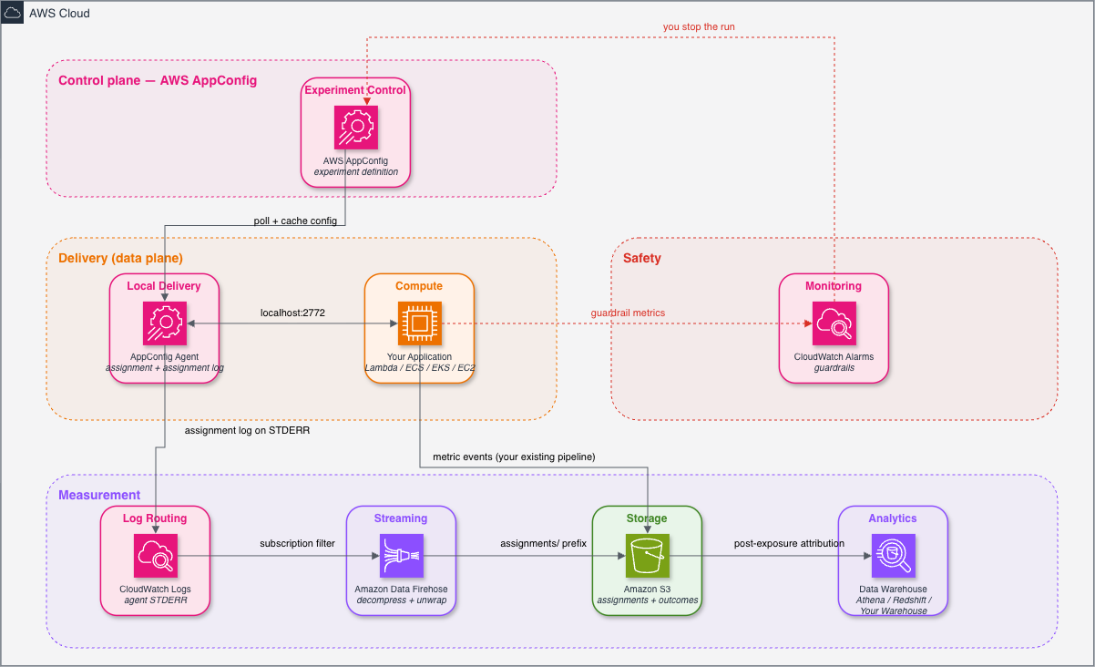
Figure 1: AWS AppConfig experimentation — the control plane in AWS AppConfig plus three runtime responsibilities (delivery, measurement, and safety), with the Agent’s assignment log reaching Amazon S3 through Amazon CloudWatch Logs and Amazon Data Firehose
Beyond the control plane in AWS AppConfig, where you define the experiment and its treatments, three things happen at runtime:
- Delivery (the data plane). The AWS AppConfig Agent retrieves the feature flag configuration from AWS AppConfig, caches it locally, and asynchronously polls for updates. Your application asks the agent for a flag over the local HTTP endpoint (
http://localhost:2772/...), passing an entity Id and any relevant request context. The agent returns the assigned treatment. The Agent returns the same treatment for the same entity for the life of the run, so a user or instance never flips treatments mid-experiment. - Measurement. Two data sets meet here. The first is treatment assignments. The Agent writes one JSON record per assignment to standard error. Your log driver ships that record to Amazon CloudWatch Logs, and a subscription filter (matched on the record type) forwards it through Amazon Data Firehose into Amazon S3. The second is your metric events — conversions, latency, cost, and errors — which keep flowing through whatever pipeline you already run.
Note: We recommend not using sensitive information such as personally identifiable information (PII) for the entity ID, the Agent logs it verbatim. If you must, hash or pseudonymize it identically in both your assignment and metric data – the entity ID is the key that joins the two. - Safety. Amazon CloudWatch alarms watch operational and experiment metrics. If an alarm fires during a run, you stop the run, which ends exposure and returns users to the deployed configuration.
One mechanism serves a frontend team, an AI team, and a backend team, each keeping its own metrics and tooling.
Example 1 — Frontend UI Experiment
Scenario. Your team believes a redesigned “Add to cart” button will lift conversion, but you only have a hypothesis. You want to expose it to a slice of production traffic and measure real behavior.
Create the experiment (console)
The experiment definition ties an application, environment, configuration profile, and feature flag to a control and one or more treatments. Audience rules determine who is eligible, and launch criteria define what counts as success. In the AWS AppConfig console, choose Experiments, then Create experiment, and work through five steps. AI-assisted experiment design in the console can validate your setup against Amazon’s experimentation best practices, helping you catch design gaps before you start a run.
Step 1 — Document your hypothesis. Give the experiment a descriptive Experiment name (add-to-cart-redesign), state the Experiment hypothesis, and use Launch criteria to record the evidence required before you promote a winner — a minimum sample per treatment, the lift you’re looking for, and the guardrails that must not regress. Writing it down now is what makes the result interpretable weeks later, and Validate my hypothesis and launch criteria will review both before you continue. Select StoreFront as the Application name.
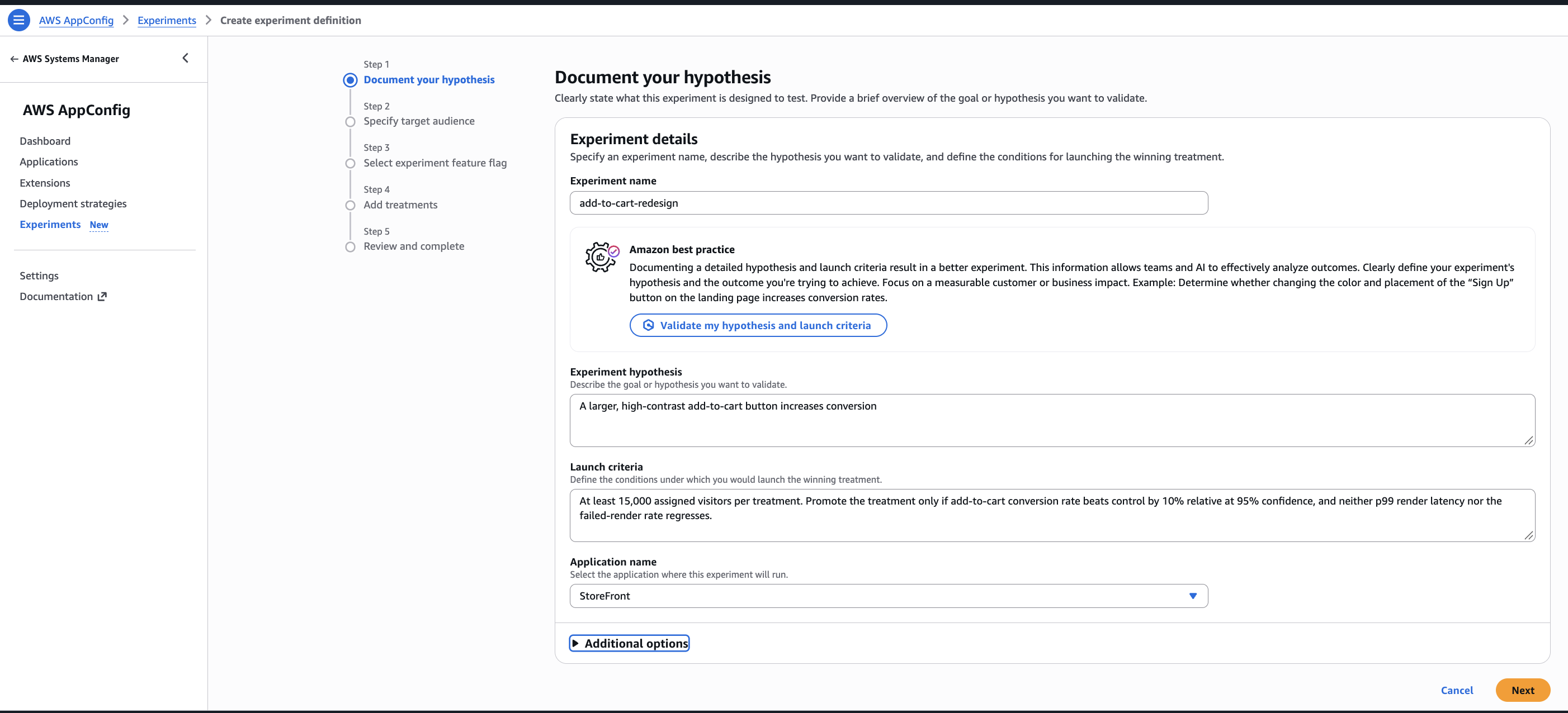 Figure 2: Documenting the hypothesis and launch criteria for the add-to-cart experiment
Step 2 — Specify target audience. Describe the audience, then build the rule. The Rule builder tab composes conditions from an attribute, an operator, and a value: $platform equals “web”, joined with And to $geo in [“USA”,”CAN”]. Sample blueprints offers pre-built rules to start from, and the Editor tab shows the same rule as an expression — the form to use if you later automate this:
(and
(eq $platform "web")
(in $geo ["USA","CAN"])
)
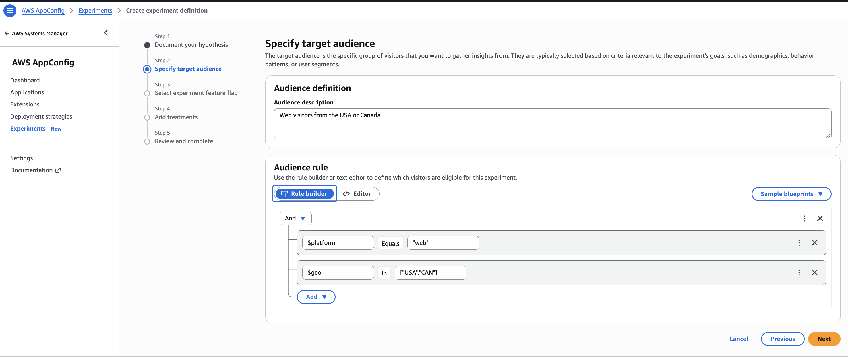
Figure 3: Building the audience rule from two conditions
That notation is an S-expression — a prefix, function-style form, (operator arg1 arg2 …). The notation is generic; AppConfig defines the operators and the $-prefixed attribute references, which are populated from the caller context your application sends. Here $geo is an attribute your application supplies — the visitor’s country, not an AWS Region.
Note: AWS AppConfig is Regional, so an experiment lives in one AWS Region — don’t use AWS Region as an audience attribute. Segment on caller properties (geography, platform, plan tier, app version); to test across Regions, replicate the experiment definition in each and measure independently.
Step 3 — Select experiment feature flag. Choose the Environment (prod), the Configuration profile holding the flag (Features), and the Feature flag itself (add_to_cart_button). The list shows flags already deployed to that environment.
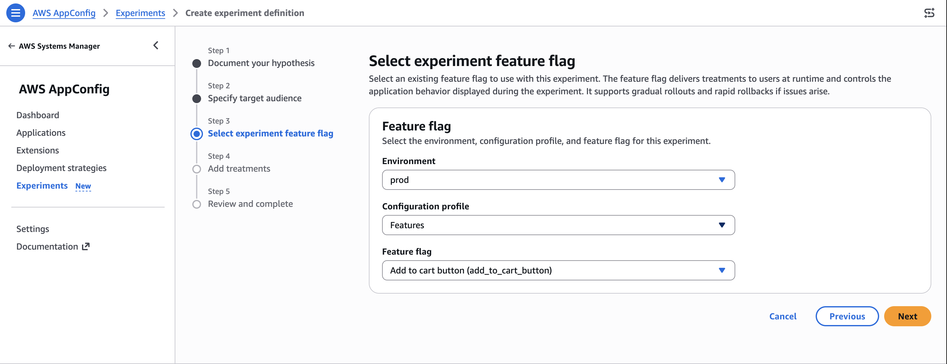 Figure 4: Selecting the deployed feature flag the experiment will control
Step 4 — Add treatments. Describe the Control as your known-good baseline, confirm its Flag value is toggled ON, and under Attribute values set button_style to classic and button_color to #232F3E. The list includes every attribute the flag defines, including ones this experiment doesn’t vary.
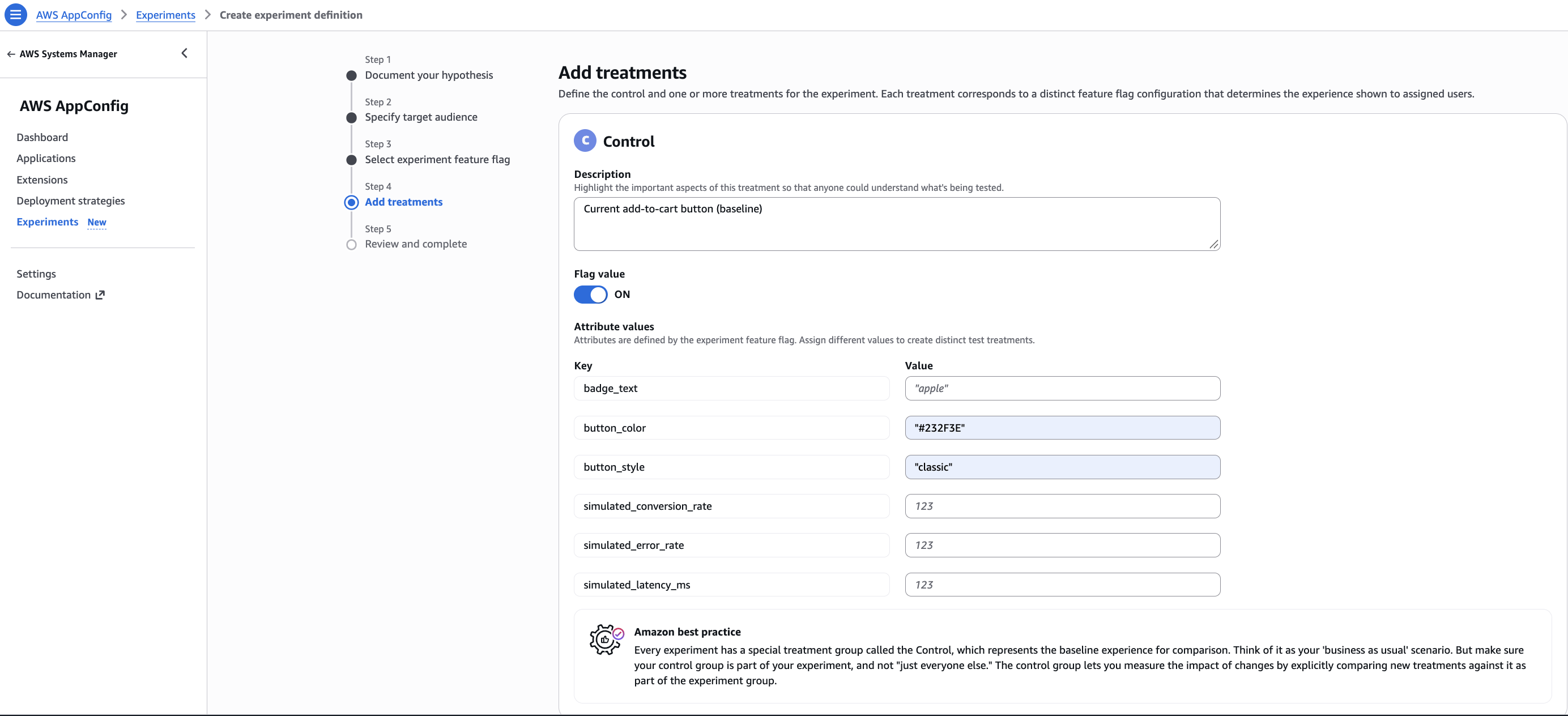 Figure 5: The control treatment, serving the current button
Then describe Treatment 1 the same way, setting button_style to prominent and button_color to #FF9900. Keep each treatment to a single change so the result stays interpretable. AppConfig allocates traffic evenly across treatments automatically — an even 50/50 here, which is also what maximizes statistical power. Advanced settings offers custom weights, but the even split is the recommended default.
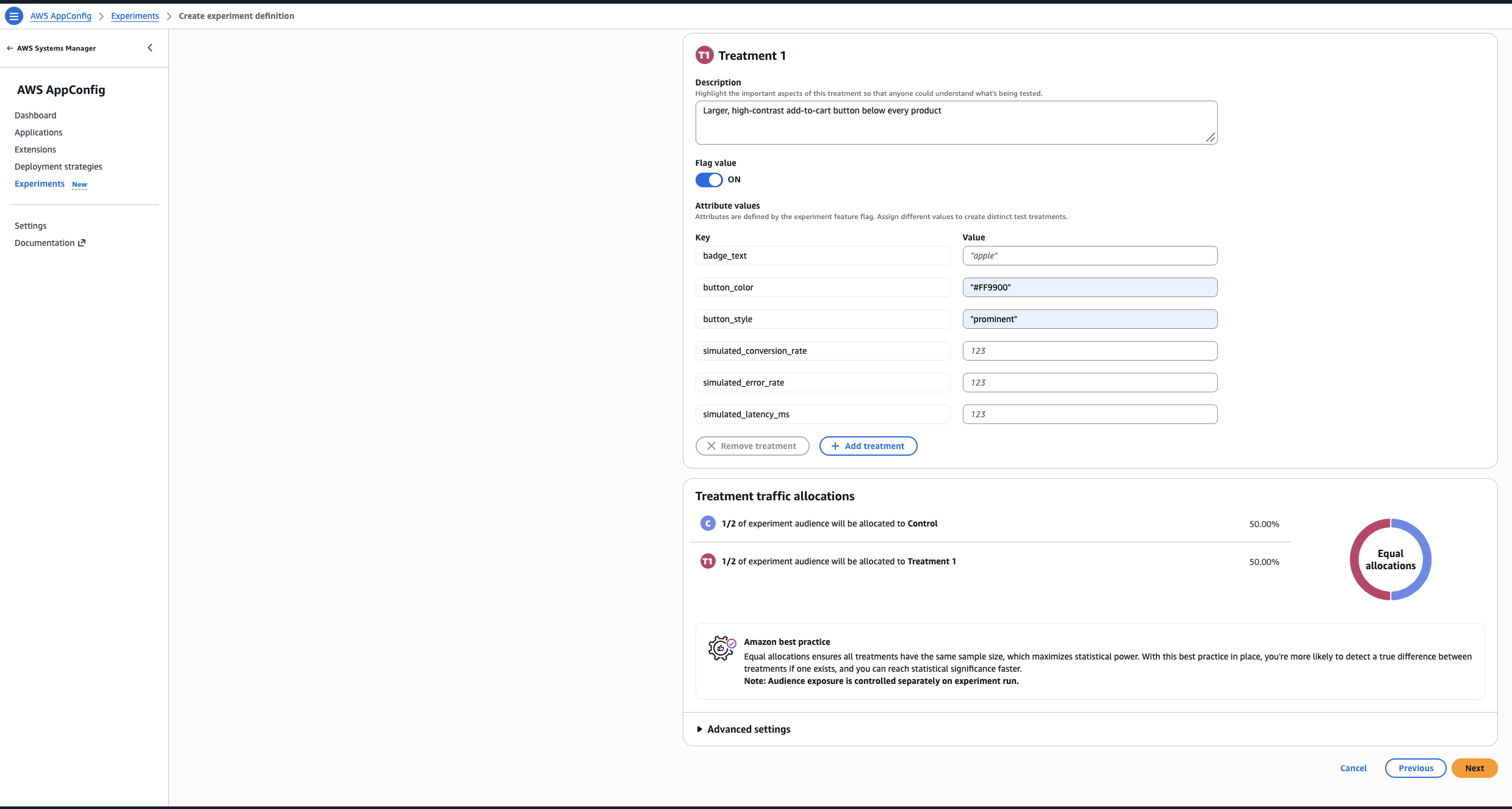 Figure 6: The treatment variant and the even traffic split
Step 5 — Review and complete. Check the summary and save. Users who aren’t assigned to the experiment continue to receive the default flag value deployed to their environment; only users in the control or a treatment are measured. AppConfig generates a treatment key for each treatment rather than deriving it from your description — it’s the value the Agent returns as _variant — and you use these keys later in treatment overrides and analysis queries.
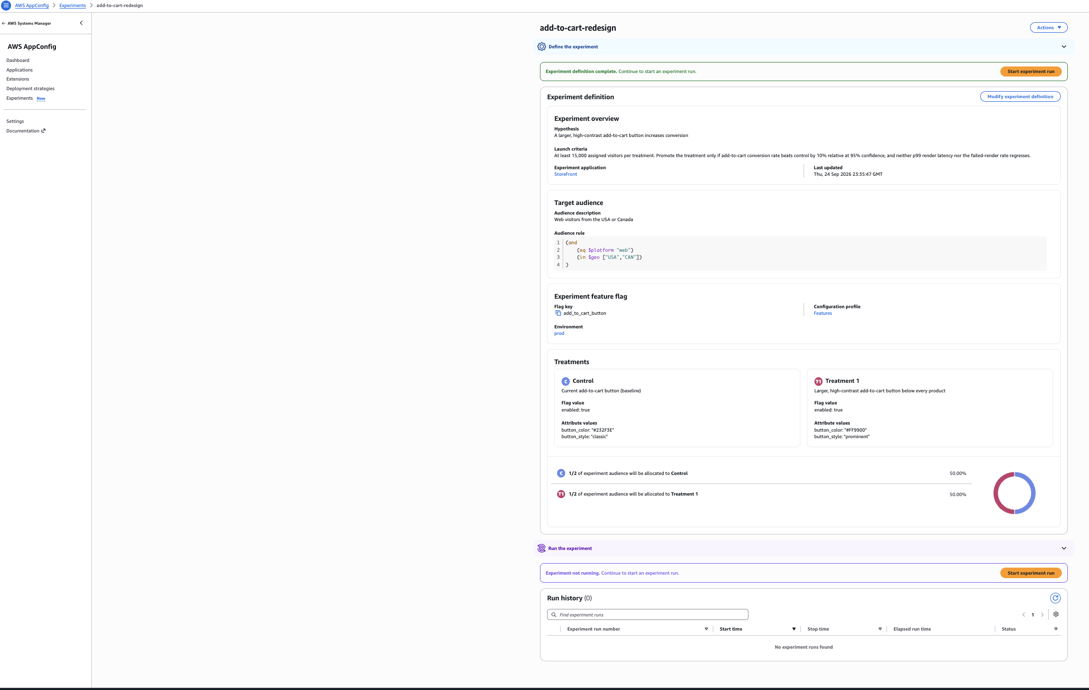 Figure 7: The saved experiment definition, ready to start a run
Retrieve the treatment (Node.js)
Your web tier asks the local AWS AppConfig Agent for the flag, passing the visitor identity as Entity-Id so the same visitor always gets the same experience, plus any context the audience rule needs. Request the flag by name with the flag parameter – if you request the whole configuration without it, no experiment assignment is recorded.
// Node.js 18 or later: fetch and Headers are globals, no imports needed.
const AGENT = "http://localhost:2772";
const PATH =
"/applications/StoreFront/environments/prod/configurations/Features";
export async function getButtonTreatment(visitorId, geo) {
// Multiple context values are sent as repeated "Context" headers,
// so use a Headers object with append (an object literal would drop
// all but the last "Context" entry).
const headers = new Headers();
headers.set("Entity-Id", visitorId); // consistent assignment for the run
headers.append("Context", "platform=web");
headers.append("Context", `geo=${geo}`);
const res = await fetch(`${AGENT}${PATH}?flag=add_to_cart_button`, {
headers,
});
// The request names a single flag, so the agent returns that flag’s
// object directly — there is no wrapper keyed by flag name:
// { "_variant": "__t1__", "enabled": true,
// "button_style": "prominent", "button_color": "#FF9900" }
return await res.json();
}
Capture treatment assignments (AWS AppConfig Agent)
The Agent logs each assignment for you – you don’t write the exposure-logging code. With EXPERIMENT_ASSIGNMENT_LOG_DESTINATION set to stderr, the Agent emits an assignment record the first time it assigns a visitor to a treatment, and that record’s timestamp is what makes clean post-exposure attribution possible later (see the Analyzing experiment results section). Your application’s job is narrower: keep producing the outcome data you already produce — add-to-cart clicks, checkouts, orders. The one thing to get right is the join key:as the Entity-Id, pass an identifier your outcomes dataset already carries — a customer ID, account ID, or session ID — so the records join with no change on your side.
# Amazon ECS, Amazon EKS, or Amazon EC2 - set this on the agent container
# or host. To collect the files yourself, use a base directory instead of
# "stderr", in the form file:/tmp/aws-appconfig/assignments/
EXPERIMENT_ASSIGNMENT_LOG_DESTINATION=stderr
# AWS Lambda - set this on the function. The extension reads the same
# setting under a prefixed name.
AWS_APPCONFIG_EXTENSION_EXPERIMENT_ASSIGNMENT_LOG_DESTINATION=stderr
# One record per assignment. Shown formatted for readability; the agent
# writes it on a single line so log shippers treat it as one event.
{
"type": "AWS.AppConfig.TreatmentAssignment",
"timestamp": "2026-07-29T16:27:55Z",
"region": "us-east-1",
"accountId": "111122223333",
"applicationId": "dn32rvt",
"experimentDefinitionId": "uioedbc",
"experimentRunNumber": "5",
"treatmentKey": "__t1__",
"entityId": "visitor-8f2c"
}
Note: The Agent’s ordinary application logs go to the same place as the assignment records, so your forwarder must match on type. Forward everything and you also forward application logs alongside the assignments and break the schema downstream.
Getting the assignment log from STDERR into Amazon S3
Three hops take you from the Agent’s standard error to something you can query. The runtime ships STDERR to Amazon CloudWatch Logs, which AWS Lambda and Amazon ECS do for you. A subscription filter forwards only the assignment records. Amazon Data Firehose writes them to Amazon S3. The first hop needs no work, so these two commands are the whole pipeline for the frontend example:
# 1. Firehose stream that lands assignment records in Amazon S3.
# The three processors are the step people miss - see the note below.
aws firehose create-delivery-stream \
--delivery-stream-name experiment-assignments \
--delivery-stream-type DirectPut \
--extended-s3-destination-configuration '{
"RoleARN": "arn:aws:iam::111122223333:role/FirehoseToS3",
"BucketARN": "arn:aws:s3:::my-experiment-data",
"Prefix": "assignments/",
"ProcessingConfiguration": {
"Enabled": true,
"Processors": [
{"Type": "Decompression",
"Parameters": [{"ParameterName": "CompressionFormat",
"ParameterValue": "GZIP"}]},
{"Type": "CloudWatchLogProcessing",
"Parameters": [{"ParameterName": "DataMessageExtraction",
"ParameterValue": "true"}]},
{"Type": "AppendDelimiterToRecord"}
]
}
}'
# 2. Forward only assignment records from the agent’s log group to that stream.
aws logs put-subscription-filter \
--log-group-name "/ecs/storefront" \
--filter-name "appconfig-treatment-assignments" \
--filter-pattern '{ $.type = "AWS.AppConfig.TreatmentAssignment" }' \
--destination-arn \
"arn:aws:firehose:us-east-1:111122223333:deliverystream/experiment-assignments" \
--role-arn "arn:aws:iam::111122223333:role/CWLtoFirehose"
Why the processors matter. CloudWatch Logs doesn’t forward events one at a time — it batches them, gzips each batch, and wraps it in an envelope. With no processing configured, your S3 objects hold compressed JSON, with each assignment record buried as an escaped string inside logEvents[].message.
Three built-in processors undo that. Decompression unzips the batch, CloudWatchLogProcessing with DataMessageExtraction discards the envelope and keeps only the message contents, and AppendDelimiterToRecord puts a newline between records so each lands on its own line. What arrives in Amazon S3 is then exactly the JSON the Agent emitted, one record per row. Leave Firehose compression off, because CloudWatch Logs has already gzipped the payload on the way in. To store Parquet, turn on Firehose data format conversion — it needs decompression enabled too.
Check it before you ramp. Treatment-assignment overrides produce no assignment records (overridden entities would pollute your results), so the 0% window can’t exercise this pipeline. Ramp to a small exposure instead, 1% is sufficient, let real assignments flow, and confirm a record lands under s3://my-experiment-data/assignments/. If the object is gzipped or the record is nested under logEvents, the processors are not configured correctly, and the analysis query later in this post will return nothing. Fix that before you ramp any further.
Amazon ECS without CloudWatch Logs. You can also skip the middle hop entirely. Run FireLens with Fluent Bit as the task’s log router, filter on the same type field, and write straight to Amazon S3. That is fewer moving parts and no envelope to unwrap, in exchange for owning the Fluent Bit configuration yourself.
Either route ends the same way: point an AWS Glue table at the S3 prefix, using the fields from the sample record above. That table is the treatment_assignments source the query in Analyzing experiment results reads, and joining it to your business data is then an ordinary SQL join on the identifier both sides already share. One naming detail to watch when you write that table definition: timestamp is a reserved word in Athena DDL, so the column has to be backtick-quoted there. Queries against the table need no quoting.
The same setup works for AI experiments. Prompt text is configuration rather than code, so a system prompt and its model parameters can live in flag attributes and be varied exactly like the button styling above — no redeploy to reword a prompt. Key the assignment on a session ID so a single conversation doesn’t switch prompts mid-thread, and treat token cost and latency as first-class guardrails, since a “better” prompt that quietly doubles spend isn’t a win.
Example 2 — Backend Cache TTL Experiment
Scenario. You suspect a longer cache TTL will cut database load without noticeably hurting freshness. This is a backend experiment, so the natural unit of assignment isn’t a user — it’s the service instance. Entity-Id set to the instance/task ID gives you stable, instance-level segmentation.
Example 1 used the console, which is the quickest way to get a first experiment running. This example uses the AWS CLI — the same definition expressed as JSON, which is what you’d reach for to script experiment creation or keep it in source control.
Create the experiment (CLI, instance-level segmentation)
aws appconfig create-experiment-definition \
--application-identifier "Catalog" \
--environment-identifier "prod" \
--configuration-profile-identifier "Features" \
--flag-key "cache_config" \
--name "cache-ttl-tuning" \
--hypothesis "A longer cache TTL reduces DB load without hurting freshness" \
--audience-rule '(eq $service "product-catalog")' \
--control file://control.json \
--treatments file://cache-treatments.json
Define the variations (JSON)
The control and each treatment are TreatmentInput objects: a FlagValue (the flag’s Enabled state plus its AttributeValues) and a Weight that sets traffic allocation. Where the console offered a plain Value field, the API takes a typed object — NumberValue for a number, StringValue for a string.
control.json:
{
"Description": "Current 60s cache TTL (baseline)",
"Weight": 50.0,
"FlagValue": { "Enabled": true, "AttributeValues": { "ttl_seconds": { "NumberValue": 60 } } }
}
cache-treatments.json:
[
{
"Description": "Increase cache TTL to 300s to reduce DB load",
"Weight": 50.0,
"FlagValue": { "Enabled": true, "AttributeValues": { "ttl_seconds": { "NumberValue": 300 } } }
}
]
Type numeric flag attributes deliberately. Define ttl_seconds as a number attribute on the feature flag with minimum and maximum constraints, and express it in whole seconds. AWS AppConfig validates attribute values when you save the configuration profile, so an out-of-range TTL fails there rather than in production.
Apply in an Amazon ECS service (Java / Spring Boot)
The AWS AppConfig Agent runs as a sidecar container in the same Amazon ECS task and is reachable at localhost:2772. Use the Amazon ECS task ID as the Entity-Id so each instance holds a consistent treatment for the whole run.
@Component
public class CacheConfigProvider {
private static final String AGENT_URL =
"http://localhost:2772/applications/Catalog/environments/prod"
+ "/configurations/Features?flag=cache_config";
private final HttpClient http = HttpClient.newHttpClient();
private final String entityId = resolveTaskId(); // instance-level unit
public CacheConfig getCacheConfig() throws Exception {
HttpRequest request = HttpRequest.newBuilder()
.uri(URI.create(AGENT_URL))
.header("Entity-Id", entityId)
.header("Context", "service=product-catalog")
.GET()
.build();
HttpResponse<String> response =
http.send(request, HttpResponse.BodyHandlers.ofString());
// single-flag request: no wrapper keyed by flag name
JsonNode flag = new ObjectMapper().readTree(response.body());
String treatment = flag.get("_variant").asText();
int ttl = flag.get("ttl_seconds").asInt();
emitMetrics(entityId, treatment); // the agent logs the assignment
return new CacheConfig(ttl, treatment);
}
private String resolveTaskId() {
// ECS injects ECS_CONTAINER_METADATA_URI_V4. A GET on
// $ECS_CONTAINER_METADATA_URI_V4/task returns the task metadata,
// whose TaskARN ends with the task ID.
try {
String metadataUri = System.getenv("ECS_CONTAINER_METADATA_URI_V4");
HttpRequest metadata = HttpRequest.newBuilder()
.uri(URI.create(metadataUri + "/task"))
.GET()
.build();
String body =
http.send(metadata, HttpResponse.BodyHandlers.ofString()).body();
String taskArn =
new ObjectMapper().readTree(body).get("TaskARN").asText();
return taskArn.substring(taskArn.lastIndexOf('/') + 1);
} catch (Exception e) {
// Fail fast. A hard-coded fallback would hand every task the same
// Entity-Id, put the whole fleet in one treatment, and quietly
// invalidate the experiment.
throw new IllegalStateException("Could not resolve the ECS task ID", e);
}
}
}
Your service then emits its guardrail metrics tagged with the same entity_id, so you can compare the 60s and 300s TTL directly.
Configuring Safety Guardrails
An experiment is a production change, so treat it like one: define what “bad” looks like before you ramp. Two controls limit the damage: gradual exposure keeps the exposure small, and Amazon CloudWatch alarms that tell you when to stop the run.
Start safe, ramp gradually. Start every run at 0% audience exposure. At 0%, no traffic is assigned unless you add treatment-assignment overrides — specific entity IDs pinned to a treatment. Use that window to validate the treatment before any real users are exposed: confirm the flag renders the expected experience for each treatment (including the control), confirm your outcome metric logging works, and share the overrides with stakeholders for a preview. For the full validation checklist, see About running and monitoring an experiment.
One thing that window can’t cover: overrides produce no assignment records, so the assignment log pipeline is only exercised once real traffic is being assigned. Clear the overrides, increase exposure in small steps, and treat that first step as the point to confirm assignment records are landing in your warehouse before you ramp further. Watch metrics at each level so a regression hits a small blast radius, not your full audience. Treat overrides as a validation tool, not audience targeting — leave production segmentation to the audience rule.
# Start the run at 0% exposure to validate before exposing any production users.
# Billing for the run begins with this call and continues until the run is stopped.
# The overrides pin named entities to a treatment so you can exercise the
# application path. Overridden entities are deliberately left out of the
# assignment log, so this window cannot validate that pipeline.
aws appconfig start-experiment-run \
--application-identifier "StoreFront" \
--experiment-definition-identifier "add-to-cart-redesign" \
--exposure-percentage 0 \
--treatment-overrides '[{"TreatmentKey": "__t1__",
"EntityIds": ["qa-jane", "qa-raj"]},
{"TreatmentKey": "__control__",
"EntityIds": ["qa-sam"]}]'
Define rollback triggers with Amazon CloudWatch alarms. Before you start a run, decide which metrics indicate unacceptable behavior and create Amazon CloudWatch alarms to watch them. Monitor those alarms throughout the run. If an alarm fires:
- Evaluate the impact and scope of the regression.
- Stop the experiment run — this ends audience exposure immediately and returns users to the currently deployed feature flag configuration.
Note that after you increase exposure, it cannot be decreased within the same run. This is intentional to prevent data corruption. To reduce exposure, stop the run and start a new one at a lower percentage.
# Example: alarm on elevated 5xx error rate to watch during the experiment.
# The dimension is not optional: without it the alarm watches a metric that
# never receives data, so it sits in INSUFFICIENT_DATA instead of firing.
aws cloudwatch put-metric-alarm \
--alarm-name "exp-add-to-cart-5xx" \
--namespace "AWS/ApplicationELB" \
--metric-name "HTTPCode_Target_5XX_Count" \
--statistic Sum \
--period 60 \
--evaluation-periods 3 \
--threshold 50 \
--comparison-operator GreaterThanThreshold \
--dimensions Name=LoadBalancer,Value=app/storefront-alb/50dc6c495c0c9188 \
--treat-missing-data notBreaching
A note on automatic rollback. AWS AppConfig environment monitors (alarms associated with an AppConfig environment) automatically roll back an unhealthy configuration deployment. They are scoped to deployments, not experiment runs:
- While a run is active, AWS AppConfig manages the flag value for assigned entities. Ending exposure requires an explicit stop-experiment-run call.
- Keep the monitors in place — you still deploy configurations during and after a run (promoting the winner is a deployment).
- Treat the alarm-and-stop-the-run pattern above as the guardrail for the experiment itself.
Choose guardrail metrics by experiment type. The right alarm depends on what you’re testing:
- Frontend/UI: page load time, client-side error rate, rendering failures, 5xx rate. A conversion lift means nothing if the page is throwing errors.
- Backend: p99 latency, throughput, error rate, and resource-specific signals (for the cache example, cache hit ratio and database load). A treatment can look neutral on business metrics while degrading system health.
Operational hygiene. Follow these rules to keep your results valid:
- Do not change treatment behavior mid-run — stop, modify, and start a new run instead, or you invalidate the data.
- Avoid shipping unrelated changes or overlapping experiments on the same audience while a run is active.
- Monitor operational metrics alongside your experiment metrics — a positive result on the headline metric can still hide a latency or error regression.
Analyzing Experiment Results
AWS AppConfig provides aggregate real-time metrics — exposure levels, treatment allocation, traffic distribution — but it doesn’t compute your results. Your metric definitions and raw data stay in your warehouse (Amazon S3 + Amazon Athena, Amazon Redshift, Snowflake, Databricks, or other) where you control exactly how success is measured.
The core principle: post-exposure attribution. Only count a user’s outcomes after the moment they were assigned to their treatment. Events before assignment don’t attribute to the experiment and bias your results. Concretely, you join your metric events to the Agent’s assignment records on entity ID, and keep only metric events whose timestamp is at or after that entity’s assignment timestamp.
Assuming the Agent’s assignment records and your metric events have landed in Amazon S3 and are queryable through Amazon Athena:
WITH assignments AS (
SELECT
entityid AS entity_id,
treatmentkey AS treatment,
MIN(from_iso8601_timestamp(timestamp)) AS assigned_at
FROM treatment_assignments -- AWS AppConfig Agent records from STDERR
WHERE type = 'AWS.AppConfig.TreatmentAssignment'
AND experimentdefinitionid = 'uioedbc'
AND experimentrunnumber = '5'
GROUP BY entityid, treatmentkey
),
attributed_conversions AS (
SELECT
a.treatment,
a.entity_id,
COUNT(m.entity_id) AS conversions
FROM assignments a
LEFT JOIN experiment_events m -- your existing outcomes table
ON m.entity_id = a.entity_id -- or m.customer_id, whichever column it already has
AND m.event_type = 'conversion'
-- post-exposure attribution: outcomes only count after assignment
AND from_iso8601_timestamp(m.timestamp) >= a.assigned_at
GROUP BY a.treatment, a.entity_id
)
SELECT
treatment,
COUNT(DISTINCT entity_id) AS assigned_users,
SUM(CASE WHEN conversions > 0 THEN 1 ELSE 0 END) AS converters,
ROUND(
SUM(CASE WHEN conversions > 0 THEN 1 ELSE 0 END) * 100.0
/ COUNT(DISTINCT entity_id), 2
) AS conversion_rate_pct
FROM attributed_conversions
GROUP BY treatment
ORDER BY conversion_rate_pct DESC;
This returns assigned users, converters, and conversion rate per treatment so you can compare each treatment against the control.
The only requirement on your outcomes data is that it carries the same identifier you passed as Entity-Id and a timestamp. Whatever table structure, column names, or warehouse you already use works — the join is on that shared identifier with a timestamp filter.
Adapting the query for other metrics. The assignments CTE and the post-exposure join are reusable; only the metric aggregation changes:
- Backend/cache experiments:
aggregate AVG(db_query_count), cache hit ratio, orapprox_percentile(latency_ms, 0.99)per treatment to confirm the longer TTL cut load without hurting p99. - Continuous metrics generally: replace the converter count with
AVG(...),SUM(...), orapprox_percentile(...)over the attributed rows.
Before you declare a winner, check three things. First, confirm each treatment reached the sample size you set in your launch criteria. Second, confirm the split matches the configured weights; a 50/50 experiment that lands at 46/54 points to an assignment or logging bug, not a result. Third, run a significance test in your statistics tooling, such as a two-proportion z-test for conversion rate. Act on the result only when all three checks pass.
Stopping an experiment and promoting a winner
Stop an experiment run when you have a clear result, when something goes wrong, or when priorities shift. Stopping ends exposure immediately. AWS AppConfig stops managing the flag and your application serves whatever configuration is currently deployed to the environment.
Promoting the winner without a gap. The order matters. If you stop first, users briefly revert to the pre-experiment default while you redeploy. To avoid that:
- While the experiment is still running, update the feature flag to match the winning treatment and deploy it. Assigned entities see no change — AWS AppConfig is still serving them their treatment.
- Stop the experiment. AppConfig releases the flag, and your application picks up the configuration you just deployed: the winner, at 100%, with no gap.
Mind what you change in step 1. Add the winning values as a variant gated by the same audience rule the experiment uses, and nobody sees a change until you stop the run. Change the flag’s default value instead and everyone outside the experiment’s audience picks up the winning value the moment the deployment lands — choose this when you want a full release.
Cost considerations and cleaning up
You pay for experiment-run hours. Billing starts when you call start-experiment-run until you stop the run. Defining experiments and treatments is free.
What drives your bill:
- Run duration. Stop the run once you have enough data to make a decision.
- Concurrent runs. Each active run bills independently. Three simultaneous experiments means three times the hourly rate.
- Your data pipeline. AWS AppConfig doesn’t charge for the assignment records the Agent emits; the pipeline that carries them does. CloudWatch Logs, Amazon Data Firehose, Amazon S3, Athena, and your guardrail alarms each bill at their normal rates — see each service’s pricing page, and AWS Systems Manager Pricing for experiment runs.
To keep costs down, estimate sample size upfront so you know roughly how long a run needs to last, and validate what you can in the 0% window before you ramp. The assignment-log pipeline is the exception: it produces records — and bills — only once real traffic is being assigned.
See AWS AppConfig experimentation pricing details here.
Clean up what you created. The run-hour charge stops only when you stop the run, and the assignment pipeline keeps billing for as long as it stays in place. When you have finished with the examples in this post, remove what you created in this order:
- Stop any running experiment run. Exposure ends immediately and the run-hour charge stops. If you are promoting a winner, deploy the winning flag value first, as described above.
- Delete the experiment definitions for both examples. ARCHIVE hides a definition but keeps its run history; DESTROY removes the definition and the history permanently.
- Take down the assignment pipeline and the alarms: the Amazon CloudWatch Logs subscription filter, the Amazon Data Firehose delivery stream, and the guardrail alarms. Then unset EXPERIMENT_ASSIGNMENT_LOG_DESTINATION on the Agent and redeploy so it stops writing assignment records.
- Decide what to do with the data. The assignment records in Amazon S3, the AWS Glue table over them, and your Athena query-results location all keep incurring storage charges. Delete them unless you want to keep the audit trail, along with the IAM roles and the log group you created only for this walkthrough.
Leave the feature flag and its configuration profile in place if your application still reads them — deleting the flag removes configuration your code depends on. Only the experiment definition has to go.
1. Stop the run – this ends exposure and the run-hour charge.
aws appconfig stop-experiment-run \
--application-identifier "StoreFront" \
--experiment-definition-identifier "add-to-cart-redesign" \
--run 5
2. Delete both definitions. Use ARCHIVE instead of DESTROY to keep the run history for future reference
# the run history for future reference.
aws appconfig delete-experiment-definition \
--application-identifier "StoreFront" \
--experiment-definition-identifier "add-to-cart-redesign" \
--delete-type DESTROY
aws appconfig delete-experiment-definition \
--application-identifier "Catalog" \
--experiment-definition-identifier "cache-ttl-tuning" \
--delete-type DESTROY
3. Remove the assignment pipeline and the guardrail alarm.
aws logs delete-subscription-filter \
--log-group-name "/ecs/storefront" \
--filter-name "appconfig-treatment-assignments"
aws firehose delete-delivery-stream \
--delivery-stream-name "experiment-assignments"
aws cloudwatch delete-alarms --alarm-names "exp-add-to-cart-5xx"
4. Optional and irreversible – drop the queryable copy of the assignment data. Substitute your own AWS Glue database name.
aws glue delete-table \
--database-name "experiments" \
--name "treatment_assignments"
aws s3 rm "s3://my-experiment-data/assignments/" --recursive
Conclusion
In this post, we took a single idea — “we have a theory, but no production evidence” — and turned it into two concrete experiments using AWS AppConfig experimentation: a frontend button redesign and a backend cache-TTL change. In each case, we created an experiment definition and expressed the control and treatments as feature-flag variants. We delivered them through the Agent with gradual exposure and alarm guardrails, and analyzed results with post-exposure attribution in our own data warehouse.
Experimentation becomes part of the AWS AppConfig workflow you already use, and you keep ownership of your metrics, analysis, and data. You pay per experiment-run hour, so your cost grows with how much you test.
To go deeper, start with the AWS AppConfig experimentation documentation, review running and monitoring an experiment for guardrail best practices and try the hands-on workshop.
If you have questions or feedback, leave a comment on this post. To get started, open the AWS AppConfig console and create your first experiment definition.
Running multi-day AZ evacuation drills with ARC Zonal Shift
Post Syndicated from Antoine Boucherie original https://aws.amazon.com/blogs/architecture/running-multi-day-az-evacuation-drills-with-arc-zonal-shift/
Running a multi-day Availability Zone evacuation drill with ARC Zonal Shift is an effective way to prove your application can withstand a sustained impairment. Multi-Availability Zone deployment is an architectural best practice for building resilient applications on AWS, but there is a gap between deploying multi-AZ and proving it works under sustained stress. Traditional disaster recovery (DR) tests validate the failover mechanism. A typical test shifts traffic, confirms targets respond, and rolls back within minutes. These short exercises don’t surface the issues that only appear over hours or days.
A multi-day AZ evacuation forces time-dependent behaviors to play out completely, exposing failure modes that brief tests miss:
- Auto Scaling policies that aren’t tuned for sustained N-1 operation over a full day.
- Deployment pipelines that don’t validate AZ health before placing new workloads.
- Stale DNS or cached database endpoints.
- Time-based routine operational processes tested against an N-1 architecture (certificate rotations, credential and secret rotations, maintenance windows, log rotation, backup automation, and cron jobs).
- Long-lived database connections pinned to a specific AZ that are only used infrequently.
- Recovery after a sustained multi-day shift, which is a different operational procedure than rolling back to a warm, nearly identical AZ within minutes.
By shifting all traffic away from a single AZ for 48–72 hours using Amazon Application Recovery Controller (ARC) Zonal Shift, you force your architecture to sustain full production load on N-1 zones. This proves capacity sufficiency, database stability, and client reconnection behavior, but most importantly, that your teams can operate normally for days on N-1 capacity.
This post shows you how to plan and run a multi-day AZ evacuation drill across Amazon Elastic Container Service (Amazon ECS), Amazon Elastic Kubernetes Service (Amazon EKS), Amazon Relational Database Service (Amazon RDS) for PostgreSQL, and Amazon Aurora PostgreSQL, with step-by-step CLI commands, a prerequisites section, observability metrics, and restore procedures.
Why financial services institutions are doing this already
Financial services organizations face unique regulatory pressure to demonstrate, not just document, their disaster recovery capabilities. Across the world, there is an increasing focus on building and demonstrating operational resilience within regulated entities. This is shifting the mindset from “show us your runbook” to “show us the evidence”. This uplift in control environments is driving financial services companies to conduct live DR testing under realistic conditions and produce auditable proof of recovery within defined timeframes. Some insurers and banks are now running periodic AZ evacuation drills as part of their operational resilience programs, shifting from “we have multi-AZ” to “we have proven multi-AZ”. Using ARC Zonal Shift, you can shift traffic at the infrastructure layer without changing application code. It works natively across Application Load Balancer, Network Load Balancer, Amazon Elastic Compute Cloud (Amazon EC2) Auto Scaling groups, and Amazon EKS clusters.
Solution overview
In this walkthrough, we demonstrate how to evacuate an Availability Zone for a multi-tier digital platform running on AWS.
We deliberately include both ECS and EKS, and two database engines, to show the evacuation procedure for each major service type readers are likely to run. The architecture is illustrative only.
The following table outlines the architecture:
| Layer | Components | Multi-AZ Configuration |
| Traffic ingress | Application Load Balancer (ALB) fronting ECS | Deployed across 3 AZs, cross-zone load balancing activated |
| Compute (containers) | Amazon ECS (Fargate) | Stateless tasks distributed across 3 AZ subnets |
| Traffic ingress | Network Load Balancer (NLB) fronting EKS | Deployed across 3 AZs, cross-zone load balancing activated |
| Compute (Kubernetes) | Amazon EKS or EKS Auto Mode | Stateless services with topology spread constraints across 3 AZs |
| Database | Amazon RDS for PostgreSQL | Multi-AZ: primary in AZ A, standby in AZ B |
| Database | Amazon Aurora PostgreSQL | Writer in AZ A, reader in AZ B. Storage replicated across all 3 AZs |
Note that the Aurora storage layer differs from standard RDS Multi-AZ. Aurora synchronously replicates data to six storage nodes across Availability Zones independently of compute instances, so only the writer or reader instance needs to be failed over as the storage remains fully available throughout the drill.
In this walkthrough, we evacuate AZ A, the zone hosting the RDS primary and Aurora writer.
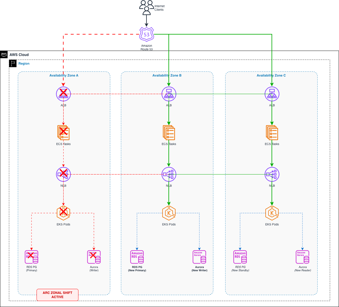
How ARC Zonal Shift works
When you initiate a zonal shift, ARC takes two coordinated actions for Amazon Route 53 and Elastic Load Balancers:
- DNS removal: The load balancer’s IP address in the affected AZ is removed from DNS. New client queries don’t resolve to that endpoint.
- Cross-zone traffic blocking: Load balancer nodes in the remaining AZs stop routing requests to targets in the shifted AZ, even when cross-zone load balancing is enabled.
For Amazon EKS clusters with zonal shift enabled, ARC goes further. It performs the following actions:
- Cordons all nodes in the impacted AZ, preventing new pod scheduling.
- Removes pod endpoints in the impacted AZ from EndpointSlice resources, redirecting east-west service-to-service traffic to healthy AZs.
- Suspends AZ rebalancing for managed node groups and updates ASGs to launch instances only in healthy AZs.
- Preserves nodes and pods in the shifted AZ (they are not terminated), keeping full capacity available for when the shift ends.
Combined with service-specific procedures for ECS task redistribution and database failover, this creates a complete AZ evacuation across all three traffic dimensions: north-south ingress, east-west service communication, and outbound database connections.
ARC Zonal Shift is a data plane operation by design. Because it works independently of the AWS control plane, it remains available even during an AZ impairment. The other steps in this walkthrough (ECS service updates, manual RDS failovers, manual Aurora failovers, subnet group modifications) are control plane operations. For a planned drill, this distinction has no practical impact because the control plane is healthy. During a real AZ impairment, prioritize the data plane action (start the zonal shift first to stop traffic immediately) and perform control plane operations only after traffic has already been shifted.
Prerequisites
Configure these prerequisites well in advance of your first shift. These are foundational settings that verify that your architecture is shift-ready at all times. For this walkthrough, you should have the following:
- An AWS account
- A multi-tier application deployed across 3 Availability Zones with ALB/NLB, ECS or EKS workloads, and RDS or Aurora databases.
- IAM permissions to manage ARC Zonal Shift, ECS, EKS, and RDS resources.
- AWS Command Line Interface (AWS CLI) v2 installed and configured.
- Familiarity with ARC Zonal Shift concepts.
- Amazon CloudWatch dashboards with per-AZ metric breakdowns (fault rate, latency, and target health).
- Auto Scaling policies validated for sustained N-1 AZ operation.
Specifically for Elastic Load Balancing (ELB):
- ALB/NLB deregistration delay set to 60 seconds, which allows existing connections to drain quickly after a shift instead of the default 300 seconds.
target_group_health.dns_failover.minimum_healthy_targets.countconfigured on each target group.
Specifically, for EKS:
- kubectl installed and configured for your EKS cluster.
- Turn on Topology Aware Routing on EKS services (or configure Istio locality-aware load balancing).
- Zonal shift activated on your EKS cluster (one-time setup).
Specifically, for ECS:
- ECS
stopTimeoutset to 55 seconds in task definitions, slightly below the ALB deregistration delay so tasks finish in-flight requests before being force-stopped, avoiding 502 errors during the drain window.
Specifically, for RDS:
- Verify that your RDS primary and standby are provisioned in different Availability Zones.
What changes for a multi-day shift
The mechanics of starting a zonal shift are the same whether you run it for 1 hour or 72 hours. What changes is the operational surface area:
- Expiry management: Zonal shifts have a maximum duration. You must monitor and extend them before they expire, or traffic returns to the shifted AZ unexpectedly.
- Scaling drift: Over days, Auto Scaling events in healthy AZs may create capacity imbalances. Monitor and cap scaling so recovery doesn’t overload the returning AZ.
- Connection pool cycling: After 24+ hours, most client connections will have recycled. This validates DNS TTL compliance across your entire client fleet, something a 1-hour test won’t fully exercise.
- Operational confidence: Teams will learn to deploy, patch, and troubleshoot in a reduced AZ environment. A multi-day drill forces this to happen naturally rather than in a controlled window.
- Safe recovery: After days at N-1 capacity, restoring the shifted AZ requires careful ordering. Verify health, scale back gradually, and reintroduce traffic incrementally rather than all at once.
Solution details
Each section below walks through the zonal shift procedure for one layer of the architecture, starting with the compute tier and finishing at the database layer.
Amazon ECS — Zonal Shift with task redistribution
For ECS services behind an ALB, initiating a zonal shift at the load balancer layer stops new traffic from reaching targets in the evacuated AZ. Existing ECS tasks in that AZ remain running but stop receiving requests. To perform a complete evacuation, follow these steps:
Step 0. Before starting, verify ARC Zonal Shift is enabled on the load balancer (disabled by default)
Step 1. Initiate the zonal shift on the load balancer.
Zonal shifts expire after the duration set in --expires-in. If the shift expires before you cancel it, traffic automatically returns to the shifted AZ. For a multi-day drill, monitor the remaining time and extend before expiry using:
When cross-zone load balancing is enabled (the default for ALB), the shift instructs load balancer nodes in healthy AZs not to route requests to targets in the impaired AZ. Targets are fully isolated regardless of your cross-zone configuration.
Step 2. Restrict new task placement to healthy AZs.
Update the ECS service’s network configuration to exclude subnets in the evacuated AZ. This prevents new tasks from launching in the shifted zone:
Step 3. If needed, scale to verify N-1 AZ capacity.
Note: updating the ECS service network configuration and count that you want are control plane operations. Perform these changes before the drill starts, not during a real AZ impairment when control plane availability may be degraded.
We recommend that you pre-scale your services to handle the loss of an AZ’s worth of capacity before the drill. Your architecture should tolerate AZ loss without needing to scale reactively. See static stability in the Amazon Builders’ library.
In a 3 AZ environment, pre-scaling for N-1 capacity means running approximately 50% more compute than your baseline peak requires. If the cost isn’t justifiable for all workloads, consider scheduled scaling policies that increase capacity during planned drill windows, Auto Scaling with aggressive scale-out thresholds, or load shedding mechanisms. Keep in mind that during an unplanned impairment, you won’t have time to scale reactively. Workloads that aren’t pre-scaled will operate in a degraded state until scaling catches up, which can take minutes under load.
Step 4. Monitor task distribution.
Restore: Revert the network configuration to include all three AZ subnets, then cancel the zonal shift. Tasks will gradually rebalance across all AZs during subsequent deployments.
Important: zonal shift won’t work for single-AZ target groups as the ALB will refuse the shift if healthy targets only exist in one Availability Zone. Verify each target group has targets registered in at least two AZs before proceeding. For more details, refer to Application Load Balancers in the ARC documentation.
Amazon EKS — Zonal Shift with EndpointSlice isolation
Amazon EKS natively supports ARC zonal shift. When you turn on this capability and trigger a shift, ARC handles both the infrastructure and Kubernetes networking layers automatically.
What ARC does when you shift an EKS cluster:
- Nodes in the impacted AZ are cordoned (no new pod scheduling).
- The built-in Kubernetes EndpointSlice controller removes pod endpoints in the impacted AZ, so east-west service traffic is automatically redirected to pods in healthy AZs.
- For managed node groups, AZ rebalancing is suspended and ASGs are updated to only launch in healthy AZs.
- Nodes and pods in the shifted AZ are not terminated, ensuring full capacity is immediately available when the shift ends.
Step 1. Activate zonal shift for your EKS cluster (one-time setup):
Step 2. Start the zonal shift on both the load balancer and EKS cluster:
Step 3. Verify EndpointSlice update: confirm pods in the shifted AZ are no longer receiving traffic:
Step 4. Verify node and pod status:
Verify your pods use topologySpreadConstraints with maxSkew: 1 on topology.kubernetes.io/zone and are pre-scaled to handle N-1 AZ load. The zonal shift doesn’t evict pods or trigger autoscaling by itself.
Note that ARC zonal shift doesn’t control outbound connections from pods to external dependencies like Amazon RDS. If your pods connect to AZ-specific database endpoints, consider using Istio with locality-aware routing. For implementation details, refer to End-to-end recovery from AZ impairments in EKS using Zonal Shift and Istio.
For Aurora, the cluster endpoint automatically routes to the current writer regardless of AZ, so no Istio configuration is needed for writer traffic. However, if you use AZ-specific reader instance endpoints, configure Istio ServiceEntry resources for each endpoint and apply a DestinationRule with localityLbSetting to prefer healthy AZs. This directs outbound database traffic to follow the same shift pattern as your north-south and east-west traffic.
Restore: Cancel both zonal shifts. ARC automatically uncordons nodes, adds pod endpoints back to EndpointSlices, and restores AZ rebalancing. Traffic returns to all three AZs with full capacity already in place.
Amazon RDS for PostgreSQL — multi-AZ failover
Regarding Amazon RDS for PostgreSQL in a Multi-AZ deployment, if the primary instance resides in the AZ being evacuated, you must trigger a failover to the synchronous standby. RDS handles this through a reboot with failover.
Prerequisite: verify your RDS primary and standby are provisioned in different Availability Zones. If both are in the same zone, the following steps wouldn’t evacuate the zone as intended.
Step 1. Check current primary location:
Step 2. If the primary is in the evacuated AZ, manually force failover:
Step 3. Wait for availability and verify the new primary AZ:
After failover, RDS recreates the standby in the evacuated AZ automatically. This is acceptable for a sustained drill as the standby receives no client traffic. Monitor ReplicaLag to confirm replication health.
Step 4. (Optional) Remove the standby from the evacuated AZ.
If you want zero RDS presence in the evacuated Availability Zone, you can relocate the standby by modifying the DB subnet group:
- Create a manual snapshot as a safety net.
- Disable Multi-AZ on the instance.
- Modify the DB subnet group to include only healthy AZ subnets, removing the evacuated AZ subnet.
- Re-enable Multi-AZ so the new standby is created in one of the remaining healthy AZs.
This approach works the same way for Amazon RDS for PostgreSQL as it does for any RDS engine using Multi-AZ deployments. Note that RDS Multi-AZ modifications (disabling/re-enabling Multi-AZ, subnet group changes) can take several minutes to complete. Plan for this during the drill window.
Amazon Aurora PostgreSQL — writer failover & reader management
Aurora provides more control over AZ placement than standard RDS Multi-AZ. You can explicitly choose which reader to promote and manage reader placement across AZs using failover priority tiers.
Step 1. Identify the cluster topology:
Step 2. If the writer is in the evacuated AZ, failover to a reader in a healthy AZ:
Step 3. Wait for the cluster to stabilize:
If your Aurora cluster has no pre-existing reader in a healthy AZ, writer promotion requires creating a new instance, which typically takes less than 10 minutes. Pre-provisioning a reader in a separate AZ reduces failover time, often to less than 30 seconds.
Step 4. (Optional) Remove the reader in the evacuated AZ and create one in a healthy AZ.
For a full AZ evacuation where you want zero database presence in the shifted zone:
Step 5. Monitor replication and performance throughout the drill:
Monitoring the drill with CloudWatch
A multi-day drill is only as valuable as the evidence it produces. Unlike a brief failover test where you visually confirm targets respond, a 48–72-hour evacuation requires continuous, automated observation, capturing capacity trends, replication health, and latency shifts that only surface under sustained N-1 AZ load.
Before starting the drill, verify you have CloudWatch dashboards with per-AZ metric breakdowns for each layer of your architecture. During the drill, these metrics serve two purposes: real-time operational awareness and post-drill evidence for stakeholders.
Key metrics by layer
The following metrics give you real-time visibility into each layer of the architecture during the drill.
Application Load Balancer / Network Load Balancer
| Metric | Dimension | What to watch |
| HealthyHostCount | Per target group, per AZ | Should drop to 0 in evacuated AZ. Stable in healthy AZs |
| UnHealthyHostCount | Per target group, per AZ | Targets in evacuated AZ may show unhealthy (expected) |
| RequestCount | Per AZ | Zero traffic in shifted AZ. Even distribution in remaining AZs |
| TargetResponseTime | Per AZ | Watch for latency increases in healthy AZs under concentrated load |
| HTTPCode_Target_5XX_Count | Per target group | Sustained increase signals capacity pressure |
Amazon ECS
| Metric | Dimension | What to watch |
| CPUUtilization | Per service | Should not exceed 70–80% sustained (indicates capacity headroom) |
| MemoryUtilization | Per service | Memory pressure under concentrated load |
| RunningTaskCount | Per service | Confirms tasks running only in healthy AZs |
| DesiredTaskCount vs RunningTaskCount | Per service | Gap indicates placement failures (check subnet/capacity) |
Amazon EKS (using Container Insights)
| Metric | Dimension | What to watch |
| node_cpu_utilization | Per node, filtered by AZ | Nodes in healthy AZs absorbing shifted load |
| pod_cpu_utilization | Per pod/namespace | Hotspot detection under N-1 operation |
| node_status_condition | Per node | Nodes in evacuated AZ should show SchedulingDisabled |
| pod_number_of_container_restarts | Per pod | Restart loops may indicate resource pressure |
Amazon RDS for PostgreSQL
| Metric | Dimension | What to watch |
| CPUUtilization | Per instance | Primary under higher load post-failover |
| DatabaseConnections | Per instance | Connection spike after failover (watch for pool exhaustion) |
| ReadIOPS / WriteIOPS | Per instance | I/O patterns shift when primary moves AZs |
| ReplicaLag | Per standby | Should stabilize within seconds after failover |
| FreeableMemory | Per instance | Memory pressure under full client reconnection |
Amazon Aurora PostgreSQL
| Metric | Dimension | What to watch |
| AuroraReplicaLag | Per reader instance | Establish your cluster baseline during normal operation. Sustained increases from baseline indicate storage pressure. Aurora Replicas typically lag 100 ms or less |
| CommitLatency | Per writer | Increased commit latency indicates write contention |
| BufferCacheHitRatio | Per instance | Drop below 99% may indicate working set doesn’t fit in memory |
| DatabaseConnections | Per instance | Client reconnection behavior after writer promotion |
| VolumeBytesUsed | Per cluster | Aurora storage is AZ-independent (should be unaffected) |
Export your per-AZ CloudWatch dashboards as snapshots before, during, and after the drill. Combine these with the ARC zonal shift event history (available through list-zonal-shifts) to create an auditable evidence package.
Cleaning up
After completing the drill, restore services carefully. The order matters, especially if Auto Scaling has increased capacity in healthy AZs:
- Verify the evacuated AZ is healthy: confirm targets are registered, pods are running, and database instances are available.
- Cancel the EKS cluster zonal shift first (east-west traffic resumes). Monitor for errors as internal traffic rebalances.
- Cancel the load balancer zonal shift (north-south traffic resumes). Traffic returns gradually as DNS propagates.
- If Auto Scaling added capacity in the remaining AZs, scale back gradually over 15 to 30 minutes. Don’t remove capacity before traffic has redistributed evenly.
- If cross-zone load balancing is disabled, verify
target_group_health.dns_failover.minimum_healthy_targets.countis configured. This allows Route 53 to only route traffic to an AZ once it has enough healthy targets registered, preventing the restored zone from receiving traffic before it’s ready to handle it. - Monitor per-AZ metrics for 30 minutes after restoring to confirm even distribution and no error spikes.
No additional AWS resources are created by ARC Zonal Shift that incur ongoing charges. The zonal shift itself is available at no additional cost.
Conclusion
In this post, you learned how to run a sustained AZ evacuation drill using ARC Zonal Shift across Amazon Elastic Container Service (Amazon ECS), Amazon Elastic Kubernetes Service (Amazon EKS), Amazon RDS for PostgreSQL, and Amazon Aurora. By operating on N-1 Availability Zones for 48–72 hours, rather than a brief failover test, you produce evidence that your multi-AZ architecture delivers genuine, sustained resilience. This is particularly valuable for financial services organizations facing regulatory mandates that require demonstrated recovery capabilities.
To get started, use the prerequisites checklist and step-by-step procedures in this post. Begin in non-production, progress to production during low-traffic windows, and build toward sustained operation under shift. As confidence grows, activate zonal autoshift so AWS can shift traffic automatically when internal telemetry detects an impairment.
You can also use AWS Resilience Hub to assess your application’s resilience posture before and after the drill. It validates that your architecture meets your defined Recovery Time Objective (RTO) and Recovery Point Objective (RPO) targets.
Related resources
Amazon Application Recovery Controller – Zonal Shift
Best practices for zonal shifts in ARC
Using cross-zone load balancing with zonal shift
New AWS Fault Injection Service recovery action for zonal autoshift
End-to-end recovery from AZ impairments in Amazon EKS using EKS Zonal Shift and Istio
Amazon EKS now supports Amazon Application Recovery Controller
About the authors
How MHK built a HIPAA-eligible agentic AI solution on Amazon Bedrock
Post Syndicated from Deepti Tirumala original https://aws.amazon.com/blogs/architecture/how-mhk-built-a-hipaa-eligible-agentic-ai-solution-on-amazon-bedrock/
Healthcare organizations face an increasingly complex challenge: processing vast volumes of medical documents, including clinical records, claims, prior authorizations, appeals, and pharmacy data, while maintaining strict HIPAA compliance and security standards. Traditional approaches require dedicated engineering teams to build individual AI systems for each use case, each needing its own compliance infrastructure, audit trails, and security controls. Agentic frameworks that can scale across use cases can reduce lengthy development cycles and high operational overhead.
MHK, a Hearst Health company ranked #1 in payer care management solutions in the 2024 Best in KLAS: Software & Services Report, faced this exact challenge. Their medical management solution serves health plans across multiple workflows (medical, pharmacy, grievance, and appeals), each requiring intelligent document processing and decision support. Building separate AI systems for each workflow was unsustainable as demand grew.
To solve this, they developed the SmartProminence AI Orchestrator, a HIPAA-eligible agentic workflow framework built on AWS that reduced manual medical review effort by 90%. New AI features that previously took 3+ months to deploy now ship in 2 weeks.
In this post, we walk through how MHK architected this solution using Amazon Bedrock, Amazon Elastic Container Service (Amazon ECS), and event-driven patterns to create a reusable, multi-tenant orchestrator for healthcare AI.
MHK uses Amazon Bedrock exclusively for foundation model inference. They built their own orchestration, retrieval, and validation layers because healthcare workflows require domain-specific controls: DAG-based multi-step execution, clinical document retrieval tied to case context, and HIPAA-specific validation logic that goes beyond general-purpose guardrails. This approach keeps Bedrock focused on scalable model access while MHK retains full control over workflow behavior and compliance enforcement.
Background
MHK provides healthcare cost management and compliance solutions to health plans across the United States. Their medical management system supports the full lifecycle of care decisions, from the moment a provider submits a request for service through final resolution. This includes prior authorization, claims adjudication, appeals processing, pharmacy benefit verification, and medical director reviews.
Each workflow involves analyzing unstructured medical documents such as clinical notes, lab results, imaging reports, and multi-page faxed records, against structured policy criteria. Before MHK’s SmartProminence AI Orchestrator, case managers spent 5 to 10 minutes manually processing each incoming document, while medical directors spent longer reviewing complex cases that required policy adherence determinations.
MHK needed to automate this research while maintaining healthcare’s audit trail and compliance requirements, and to do so across all product modules without building separate AI infrastructure for each one.
Business challenge
As MHK evaluated how to bring AI capabilities across their entire product suite, three core challenges emerged.
- Fragmented AI infrastructure. Each AI-powered feature would require its own deployment pipeline, HIPAA compliance certification, security controls, and monitoring. Every new AI roadmap item meant a new cluster, a new compliance engagement, and a new operational burden. For a company serving multiple health plans across multiple modules, this approach could not scale.
- Lengthy development cycles. Deploying a new AI workflow through traditional engineering took 3 to 6 months, not including requirements gathering. The engineering team could not keep pace with the product roadmap.
- Manual effort at premium cost. Case managers, nurses, pharmacists, and medical directors spent hours per case manually searching through patient records. The cost was especially acute for medical directors (physicians) and pharmacists, whose hourly rates make even small-time savings translate into significant ROI.
Solution overview: SmartProminence AI Orchestrator
MHK built the SmartProminence AI Orchestrator, a multi-tenant, agentic workflow framework running entirely on AWS. Rather than building separate AI systems for each use case, MHK created a single orchestrator where various AI workflows can be deployed through configuration. Define your prompts, specify your input/output schemas, and register the agent. The solution handles everything else including HIPAA compliance, encryption, audit trails, scaling, and orchestration.
The solution is architected around a controller-agent pattern in which a Workflow Engine Controller resolves workflow dependencies and dispatches individual steps to LLM processing agents. The entire system is stateless, event-driven, and independently scalable.
The following diagram illustrates the high-level architecture of the solution.
Figure 1: MHK SmartProminence AI Orchestrator architecture on AWS
At the core of the architecture, the Agent Orchestration Core serves as the central nervous system. Built on Spring Boot and running on AWS Fargate, it exposes a REST API that handles job submission, workflow management, LLM proxying, and token management. Critically, it is the only component that directly accesses the database: controllers and agents interact exclusively through the orchestration core’s API, enforcing strict data access boundaries.
Architecture overview
This section examines the key architectural patterns the orchestrator uses to process diverse healthcare workflows at scale.
Controller-agent pattern with Amazon Bedrock
MHK selected Amazon Bedrock for its multi-model access through a single API, letting them choose the best model per workflow step without separate integrations. As a managed AWS service, Bedrock inherits existing AWS Identity and Access Management (IAM), Amazon Virtual Private Cloud (Amazon VPC), and encryption controls, avoiding a new trust boundary. Built-in content filtering and invocation logging satisfy healthcare auditability requirements, and its model-agnostic architecture lets MHK adopt newer models without rearchitecting the solution.
The orchestrator enforces a strict separation between workflow orchestration and LLM processing. The Workflow Engine Controller determines what needs to happen and in what order, while LLM processing agents execute individual steps. This separation lets agent processing scale independently from workflow logic, and it makes the workflow the single source of truth while agents operate only on specific, actionable steps.
When a job arrives, the controller loads the version-pinned workflow definition, resolves step dependencies into a DAG using Kahn’s algorithm, and pre-creates step executions in a WAITING state. It uses conditional Spring Expression Language (SpEL) expressions to decide which steps to run versus skip, then dispatches agents layer by layer. Steps at the same depth run in parallel, and the controller polls for completion before advancing to the next depth.
Each agent runs a standardized pipeline: input binding (resolving expressions to gather prior step results), optional vision processing for scanned documents, prompt assembly with enriched context, LLM invocation to Amazon Bedrock (Claude), and post-processing for field extraction, type coercion, and structured output.
For parallel workloads within a single step, agents use Java virtual threads for each execution. This lets them process multiple items concurrently, such as extracting data from each page of a multi-page document simultaneously.
Event-driven orchestration with Amazon SQS
Communication between the orchestration core, controllers, and agents flows through Amazon Simple Queue Service (Amazon SQS) queues. To trigger a workflow, the orchestration core places a ControllerTaskMessage on the Controller Invoke Queue. To dispatch an individual step, it places an AgentTaskMessage on the Agent Invoke Queue. Each message is secured with a capability token scoped to only that operation’s data.
This design delivers four properties. Stateless processing means available instances can pick up pending messages. Independent scaling lets agents scale horizontally through ECS Fargate. Fault isolation keeps a failed task from blocking parallel steps, and dead letter queues capture failures. Decoupled deployment ships new agent versions without system-wide restarts.
The only blocking call in the pipeline is the LLM invocation to Amazon Bedrock. Everything else is asynchronous and event-driven, so the system can process hundreds of concurrent jobs without resource contention.
DAG-based parallel execution
The workflow engine uses depth-based parallel execution to maximize throughput. Consider a medical policy review workflow: at Depth 0, agents simultaneously extract patient demographics and pull claims history. At Depth 1, once both are complete, a policy lookup agent identifies the relevant criteria. At Depth 2, an evidence-gathering agent searches through the patient’s clinical history for documentation that satisfies each policy criterion. The controller only advances to the next depth when steps at the current depth have completed.
Conditional expressions can dynamically skip steps based on upstream results. For example, if the initial classification step determines that a case does not involve prescription drugs, the pharmacy verification step at the next depth is automatically skipped, saving both time and token costs. This conditional logic is evaluated by the controller using Spring Expression Language (SpEL) against the structured outputs of completed steps.
Dynamic agent registry
When MHK needs a new agent type, whether for a new medical management module or a new kind of analysis, the process is configuration-driven rather than engineering-driven.
A developer defines the agent configuration (prompt templates, input/output schemas, and model selection), then registers it through the orchestration core’s API. Terraform automatically provisions the supporting infrastructure: SQS queues, IAM roles, and ECS task definitions. The agent immediately becomes available for workflow step assignments, with no new compliance certification needed, since it runs within the already certified orchestrator.
This transformed MHK’s development velocity. The engineering team focuses on prompt design and workflow logic rather than infrastructure scaffolding.
Conversational memory and case association
The orchestrator maintains context across multiple workflow executions for the same patient case. Each execution returns a job ID that the upstream system associates with the case record. Over a case’s lifetime there may be three or more executions (initial intake, policy review, and appeal processing), each producing structured outputs that stay available for later executions.
Once a 30-page clinical record has been analyzed, its structured output is available for future queries on that case without re-running ingestion. When a medical director reviews an appeal weeks later, the patient’s history is already organized and searchable.
Prior context remains in Amazon Simple Storage Service (Amazon S3), encrypted with the client’s dedicated AWS Key Management Service (AWS KMS) key.
Responsible AI controls
MHK enforces safe LLM outputs through application-layer validation built into each agent’s processing pipeline. Every agent post-processes model responses against expected output schemas, cross-references extracted data with source documents to detect hallucinations, and rejects responses that fail confidence thresholds. Domain-specific checks verify that outputs reference only the patient’s own clinical records and match policy-specific medical criteria. LLM inputs and outputs are logged with full audit trails, which supports compliance review and reproducibility for every AI-assisted decision.
AWS services used
The following table summarizes the AWS services that compose the SmartProminence AI Orchestrator and the role each plays in the architecture.
| Service | Role in architecture |
| Amazon Bedrock | Foundation model inference with IAM role-based authentication |
| Amazon ECS (Fargate) | Containerized orchestration core, workflow controllers, and processing agents |
| Amazon SQS | Event-driven inter-component communication with dead letter queues for fault tolerance |
| Amazon RDS (MySQL 8.4) | Workflow definitions, execution state tracking, multi-AZ for high availability |
| Amazon S3 | Job artifacts, document storage, immutable workflow configurations (KMS encrypted) |
| AWS KMS |
Capability token signing and validation Per-client encryption keys for multi-tenant data isolation |
| Amazon Cognito | OAuth2/JWT authentication for API access and user identity |
| Amazon CloudWatch | Logging, metrics, token usage tracking, and alerting (no PHI) |
| Elastic Load Balancing | TLS 1.3-terminated application load balancer |
| Amazon VPC | Network isolation with private subnets, VPC endpoints for service access |
Security and compliance
Healthcare data demands the highest security standards, and MHK’s architecture implements defense-in-depth across every layer. The orchestrator processes protected health information (PHI) for multiple health plan clients simultaneously, making multi-tenant data isolation a foundational feature.
- Per-client encryption. Every client has their own AWS KMS key. Documents stored in Amazon S3 are double-encrypted: S3 server-side encryption plus client-specific KMS encryption. Even if a job were somehow misrouted (which the token system helps prevent), the receiving agent could not decrypt another client’s data because it would not have access to that client’s KMS key. The database layer adds row-level encryption on top of Amazon Relational Database Service (Amazon RDS) storage-level encryption, providing defense-in-depth for data at rest.
- Capability token model. A least-privilege token system limits what each component can access. A controller-scoped token can read workflow definitions and job data, dispatch agent tasks, and create step executions. An agent-scoped token can only read its step’s input, write its own result, call the LLM through the proxy, and upload artifacts. Tokens are generated per-dispatch through KMS, so even a compromised agent cannot reach data from other steps, workflows, or clients.
- Network isolation. The database subnets have no internet access. AWS service communication (Amazon S3, Amazon SQS, AWS KMS, AWS Secrets Manager, Amazon CloudWatch, Amazon Elastic Container Registry (Amazon ECR)) flows through VPC endpoints, meaning no data ever traverses the public internet. Connections use TLS 1.3 for encryption in transit.
- Compliance controls. LLM request and response bodies are not logged. Only token counts and content hashes are recorded. Workflow configurations are stored immutably in S3 for complete version history. Agents receive only the minimum context needed for their step, following the principle of data minimization.
Results and impact
The SmartProminence AI Orchestrator delivered measurable business outcomes across both MHK’s internal operations and their health plan clients.
90% reduction in manual review effort. For document intake workflows, processing time dropped from 5–10 minutes per document (manual) to under 1 minute (automated with human-in-the-loop verification). For complex medical director reviews, the system pre-gathers the relevant evidence and presents a structured summary, reducing the physician’s task from hours of document searching to a 30-second approval or denial decision.
85% faster AI feature deployment. New AI capabilities that previously required a full 3–6 month engineering release cycle now deploy in approximately 2 weeks. The engineering team defines workflow configuration and prompt logic without building custom infrastructure, compliance pipelines, or security controls for each feature.
Unified compliance posture. Instead of attesting each AI feature independently, MHK maintains a single orchestrator-level HIPAA and SOC 2 attestation that covers the agents. New agents inherit the orchestrator’s security controls automatically: per-client encryption, audit logging, token-based access, and data minimization.
Multi-tenant extensibility. Health plan clients can run AI workflows through the framework without building their own HIPAA-eligible infrastructure. Because the orchestrator is configuration-driven, MHK can onboard new use cases for existing clients or deploy entirely new health plan customers with minimal engineering effort.
Conclusion
The orchestrator’s controller-agent architecture provides a blueprint for organizations that need to scale AI capabilities across multiple use cases without multiplying their compliance burden. The key insight is that compliance infrastructure should be an orchestrator-level concern, not a per-feature concern, and that agentic orchestration patterns can be both powerful and auditable when designed with healthcare-grade security from the ground up.
Looking ahead, MHK is extending the orchestrator with conversational interfaces so case managers and medical directors can interactively query case data, using the same workflow memory and security infrastructure. The dynamic agent registry continues to grow as new medical management modules adopt AI-powered decision support. MHK is also exploring AWS Marketplace as a distribution channel to bring their HIPAA-eligible agentic framework to organizations beyond healthcare that require similar compliance thresholds.
Share your experience building HIPAA-eligible AI workflows in the comments or reach out if you’re exploring agentic architectures for regulated industries.
To learn more, get started with Amazon Bedrock and explore the Amazon Bedrock code samples to build your own agentic AI solutions on AWS.
About the authors
Exploring a Chinese MEGA City you’ve probably never heard of…
Post Syndicated from Matt Granger original https://www.youtube.com/watch?v=Lu3VkNjaIpg
Comic for 2026.09.30 – Birth Of Venus
Post Syndicated from Explosm.net original https://explosm.net/comics/birth-of-venus
New Cyanide and Happiness Comic
Amazon Aurora PostgreSQL now supports direct querying of Apache Iceberg and Parquet data in your data lake
Post Syndicated from Esra Kayabali original https://aws.amazon.com/blogs/aws/amazon-aurora-postgresql-now-supports-direct-querying-of-apache-iceberg-and-parquet-data-in-your-data-lake/
Today, we’re announcing a new capability for Amazon Aurora PostgreSQL that you can use to directly query operational data together with data stored in your data lake in Apache Iceberg and Apache Parquet formats, using your existing PostgreSQL applications and tools. By eliminating the need to extract, transform, and load (ETL) structured data from data lakes into your operational database, you can reduce operational complexity and simplify application development. You can also use Aurora PostgreSQL to query data from data lakes managed in Iceberg REST Catalog (IRC)-compatible catalogs, giving you access to data across a breadth of analytics systems without moving or duplicating it. Whether you’re powering real-time dashboards, enriching transactions with historical context, or building AI agents that reason over both live and archived data, you can now do it all through a single, familiar interface.
Previously, if your application needed to combine recent transactional data in Aurora with historical records stored in Amazon S3, a common approach was to build reverse ETL pipelines that duplicated data, increased infrastructure costs, and required ongoing engineering effort to keep everything synchronized. This challenge only grows as you increasingly embed AI agents into your applications, where it is impractical to predict and pre-replicate every dataset an agent might need.
DuckLabs, the team that maintains the DuckDB project, recently joined Amazon, and this capability is an example of how the efficiency of DuckDB is being integrated into our services. DuckDB is now embedded directly within Aurora PostgreSQL, so you can query live operational data (including uncommitted writes) alongside your data lake in a single query. Query processing stays within Aurora, with no additional network hops and no ETL pipelines that duplicate data. You can query Apache Iceberg tables managed through the AWS Glue Data Catalog, as well as Parquet and Iceberg data stored in Amazon S3 and S3 Tables. You do all of this using familiar PostgreSQL syntax and your existing applications and tools.
We’re excited to bring the speed and simplicity of DuckDB directly into Aurora PostgreSQL, so you and your agents can query and combine operational and Iceberg data using the familiar PostgreSQL applications, tools, and endpoints already in use. By building this capability around DuckDB, future improvements to the open source engine can continue to bring performance and functionality gains to Aurora and other AWS services.
What is new
This capability is supported on two Aurora PostgreSQL major versions: 17 (starting with 17.11) and 18 (starting with 18.6). To use it, you create an Aurora PostgreSQL cluster, attach an IAM role with the AuroraAnalytics feature, and enable the aurora_analytics extension. The IAM role is what gives Aurora access to your data in Amazon S3 and the AWS Glue Data Catalog. You then create foreign tables that point to your Iceberg or Parquet data in the data lake, and query them using familiar PostgreSQL syntax. You can complete this setup through the Amazon RDS console, or with any PostgreSQL client such as psql. The process is well documented in the Aurora PostgreSQL documentation.
You can query data across external IRC-compatible catalogs through AWS Glue Data Catalog federation. You register the external catalog once with Glue, and then create foreign tables for the tables you want to query, the same way you would for any Glue-native table. A single query can then join data stored in Aurora with Iceberg tables registered across multiple catalogs, so applications get a unified view without moving data or replacing your existing catalog investments.
Aurora also applies optimizations such as predicate pushdown and column pruning so that only the relevant data is read. This keeps queries efficient even as the underlying data grows. Frequently accessed data is also cached in your Aurora instance, so subsequent queries against the same data return faster. You can inspect this behavior per query using aurora_analytics_stat_statements(), which reports metrics such as rows scanned, bytes read from Amazon S3, and cache hits.
To see how direct querying works, I connected to my Aurora PostgreSQL database using psql and created the extension:
CREATE EXTENSION aurora_analytics;For my walkthrough, I set up a simple financial scenario. I have a recent_transactions table in Aurora with the last 7 days of customer transactions, and a Parquet file in Amazon S3 containing 5 years of historical transaction data. To make Aurora aware of the historical data, I created a foreign table pointing at the Parquet file in S3:
CREATE FOREIGN TABLE transaction_history ()
SERVER aurora_analytics_server
OPTIONS (
    location 's3://<my-bucket>/finance/transaction_history.parquet',
    format 'parquet'
);
Notice the empty parentheses in the CREATE FOREIGN TABLE statement. Aurora automatically reads the schema from the Parquet file metadata, so you do not need to define columns manually. For workloads with many tables, you can skip creating them one at a time: a single IMPORT FOREIGN SCHEMA statement bulk-creates foreign tables for every Iceberg or Parquet table in an AWS Glue Data Catalog database, inferring schemas automatically.
With both tables in place, I ran a single query that combines the recent operational data in Aurora with the historical data in S3:
SELECT merchant, category, amount, transaction_date, 'recent' AS source
FROM recent_transactions
WHERE customer_id = 'C-1001'
UNION ALL
SELECT merchant, category, amount, transaction_date, 'historical' AS source
FROM transaction_history
WHERE customer_id = 'C-1001'
  AND transaction_date >= CURRENT_DATE - INTERVAL '5 years'
ORDER BY transaction_date DESC
LIMIT 15;
The result shows both recent and historical transactions in a single result set. The 7 most recent rows come from Aurora, and the rest come directly from the Parquet file in S3. DuckDB handles the analytical scan of the Parquet data under the hood, while Aurora handles the operational data. That single query would have previously required a pipeline to move the historical data into the database first.
If a query pattern needs single-digit-millisecond latency, you can materialize data from the data lake into a native Aurora PostgreSQL table using familiar commands such as CREATE TABLE AS SELECT, INSERT INTO ... SELECT, or MERGE INTO. The materialized table lives in Aurora and is queried like any other PostgreSQL table, giving you a low-latency path for hot data without operating a separate ingestion pipeline. The read queries can run on any Aurora PostgreSQL instance in your cluster, whether the writer or a read replica, so you can offload analytical scans from your operational workload. The materialization commands write data into Aurora, so they run on the writer instance.
Get started today
Direct querying of Apache Iceberg and Parquet data from Amazon Aurora PostgreSQL is available today in all commercial AWS Regions and AWS GovCloud (US) Regions, at no additional charge. You pay only for the incremental Aurora compute the queries consume and Amazon S3 request costs for reading data lake files.
To learn more, visit the Amazon Aurora features page, read the Aurora PostgreSQL documentation, or try it in the Amazon RDS console. We welcome your feedback through AWS re:Post or through your usual AWS Support contacts.
Celebrating Our Newest AWS Heroes – September 2026
Post Syndicated from Taylor Jacobsen original https://aws.amazon.com/blogs/aws/celebrating-our-newest-aws-heroes-september-2026/
Today, we’re excited to introduce the newest members of the AWS Heroes program. AWS Heroes are a vibrant, worldwide group of AWS experts who go above and beyond to share knowledge, mentor others, and build thriving communities. These individuals make a real difference in helping developers and organizations succeed with AWS.
This month, we welcome three exceptional community leaders from across the globe, each bringing unique expertise and a deep commitment to empowering builders everywhere.
Avinash Shashikant Dalvi – Bengaluru, India
 Serverless Hero Avinash Shashikant Dalvi is a tech architect and co-organizer of AWS User Group Bengaluru who is focused on serverless, containers, and production-ready applications on AWS. He has delivered over 40 community talks, publishes the AWS for Product Builders newsletter, and creates technical content covering Amazon ECS, AWS Fargate, AWS Lambda, and AWS Amplify.
Joanne Skiles – Orlando, USA
 Serverless Hero Joanne Skiles is an engineering leader and educator with over 16 years of experience building full-stack systems, including serverless architecture and AI systems on AWS. She organizes the Orlando AWS User Group and teaches cloud and AI concepts through her YouTube channel, conference talks, and her podcasts Chaotic Commits and Her Career Unplugged. Joanne is also a professor in the Computer Science department at Rollins College, where she runs the Transparent Systems lab.
Xiaofei Li – Shanghai, China
 Community Hero Xiaofei Li is an AWS Golden Jacket holder and is an active community leader in the Greater China Region, leading the Kiro, Amazon Quick, and Tokyo Chinese AWS communities. He founded the Kiro Chinese User Community (5,000+ members) and initiated the Chinese localization of AWS Builder Cards across 15 cities and 3,000+ participants. Xiaofei also mentors underserved students and supports Women in Tech initiatives.
Learn More
Visit the AWS Heroes webpage if you’d like to learn more about the AWS Heroes program, or to connect with a Hero near you. To learn more about how to get involved with the AWS community, visit our AWS Builder Center.
— Taylor
Jair Bolsonaro #lastweektonight
Post Syndicated from LastWeekTonight original https://www.youtube.com/shorts/3RDtqntU5Fk
Behind the Byline: David Brooks
Post Syndicated from The Atlantic original https://www.youtube.com/shorts/NcT88YcA0Pg
XGIMI Aura 3 Max 4K 120Hz UST Projector. Rather impressive.
Post Syndicated from Techmoan original https://www.youtube.com/watch?v=KPCWngbDCoc
Accelerating AS/400 business rule extraction with Kiro: Step-by-step guide
Post Syndicated from Daniel Gray original https://aws.amazon.com/blogs/devops/accelerating-as-400-business-rule-extraction-with-kiro-step-by-step-guide/
AS/400 business rule extraction no longer requires months of manual effort. With Kiro, an agentic AI-powered development environment (spanning IDE, CLI, web, and mobile surfaces, along with the Kiro Crew workspace), you can compress the process into days. This step-by-step guide walks through the approach. Organizations face a common challenge: critical business logic embedded in extensive RPG and COBOL code bases, often maintained by a declining number of developers and subject matter experts (SMEs) with RPG expertise. The fulfillment rules and shipping logic are scattered across interconnected programs that no single person fully understands.
In this post, we walk you through a step-by-step approach for using Kiro to extract business rules from AS/400 RPG and COBOL programs, generate technical specifications, and produce modernization-ready documentation.
Extraction process challenges
Before this engagement, one of our customers faced several challenges with their existing business rules extraction process. They were planning to modernize their AS/400 order fulfillment workflow, which handled inventory validation, shipping document generation, and warehouse operations.
- Significant consulting costs for specialized AS/400 consultants.
- Time-intensive manual analysis, typically 4–6 weeks of dedicated effort.
- Documentation that becomes outdated before the team finishes writing it.
- Risk of overlooking critical business logic during modernization.
The following is the sample system flow considered to walk through the step-by-step guide.
Each program has embedded business rules, including order validation and stock allocation with warehouse priority. These programs also handle shipping weight calculations, character encoding conversion, and integration with external carrier systems. Traditional analysis would have taken 4–6 weeks per system. The effort required across consultants, technical writers, and reviewers would have been 40–80 person-hours per system.
Solution
With Kiro, an agentic AI-powered development environment, you can extract comprehensive business rules, generate technical specifications, and create modernization-ready documentation in hours, not months (as detailed in the Outcomes section).
Working autonomously across your code base, Kiro analyzes dependencies, traces execution paths, and produces detailed documentation.
The approach relies on two core Kiro capabilities:
- Steering files: Persistent instructions that guide the AI’s behavior, including project context, naming conventions, analysis standards. Configure them once and they apply to all subsequent sessions. Steering files can reference documentation templates that define the exact output format. Each subsequent analysis follows the same repeatable structure.
- Specs: A structured way to define requirements, design, and implementation tasks. Kiro executes tasks autonomously with progress tracking. Spec tasks tell Kiro which templates to use and where to save the output.
The workflow has three phases:
Phase 1 – Configure steering files to define project context, directory structure, and technical standards. Examples include “extract 10–20 lines of code context around business rules” and “map abbreviated DDS field names to business terms.” Create documentation templates that the steering files reference. These templates specify the exact output format for business rules with code snippets, pseudocode equivalents, DDS field mappings, and integration specifications.
Figure 1: Steering files provide persistent instructions that guide the analysis behavior of Kiro across sessions, configured once and applied to subsequent analyses
Phase 2 – Build a Kiro Spec with discrete, actionable tasks: analyze source files, parse DDS definitions, extract business rules, generate pseudocode, create consolidated documentation using the templates, and verify business rules against source code.
Figure 2: The Kiro Spec, showing discrete tasks that Kiro executes autonomously with progress tracking
Phase 3 – Execute the Spec and let Kiro work autonomously. Monitor progress as tasks complete, then review the generated documentation.
Important: AI-extracted rules should be reviewed by an AS/400 SME. Automated extraction might occasionally misinterpret complex or ambiguous business logic, so human validation remains essential before acting on extracted rules.
Here’s an example of what Kiro produces. Given this RPG subroutine that validates orders against the master file, Kiro generates a plain-language business rule and its pseudocode equivalent:
Rule 1.3.16: Stock Allocation
Category: Processing Subroutine: ALLCST (lines 3820-3960) Description: Allocates stock from warehouse inventory. Looks up inventory by item key, verifies sufficient available quantity, then decrements available quantity and increments reserved quantity by the order amount. Updates the inventory record.
Source Code (lines 3820-3960):
Pseudocode:
Figure 3: Kiro extracts business rules with original RPG code, pseudocode equivalents, and plain-English descriptions
The following is the DDS field mapping that translates abbreviated AS/400 field names into business terms:
1.1 ORDERMST — Order Master
| Field | Type | Length | Dec | TEXT (Business Term) | COLHDG | VALUES | Used By |
| ZIORCD | A | 8 | — | Order Code | Order / Code | — | PROG001, PROG002, PROG003, PROG004 |
| ZIPERD | P | 6 | 0 | Fulfillment Period | Fulfill / Period | — | PROG001 |
| CURPER | P | 6 | 0 | Current Period | Current / Period | — | PROG001 |
| STATUS | A | 1 | — | Order Status | Order / Status | ‘A’ ‘H’ ‘C’ ‘X’ ’ ’ | PROG001, PROG002 |
| CUSTNAME | A | 40 | — | Customer Name | Customer / Name | — | PROG001, PROG002, PROG003, PROG004 |
| WHSCD | A | 4 | — | Warehouse Code | Warehouse / Code | — | PROG001, PROG002, PROG003, PROG004 |
| ORDDTE | P | 8 | 0 | Order Date | Order / Date | — | PROG001 |
| ORDQTY | P | 7 | 0 | Order Quantity | Order / Quantity | — | PROG001 |
| SHPTYP | A | 2 | — | Shipment Type | Shipment / Type | — | PROG001 |
| PRIORT | A | 1 | — | Priority Code | Priority | ‘1’ ‘2’ ‘3’ | PROG001 |
Record Format: ORDERMST — TEXT(‘Order Master Record’)
Key: ZIORCD (unique)
STATUS Values: A = Active, H = Hold, C = Complete, X = Canceled, ’ ’ = New/Blank
PRIORT Values: 1 = High (requires MGR session), 2 = Medium, 3 = Low
1.2 INVSTOCK — Inventory Stock Levels
| Field | Type | Length | Dec | TEXT (Business Term) | COLHDG | VALUES | Used By |
| ITEMCD | A | 10 | — | Item Code | Item / Code | — | PROG001, PROG004 |
| WHSCD | A | 4 | — | Warehouse Code | Warehouse / Code | — | PROG001, PROG004 |
| QTYOH | P | 9 | 0 | Quantity On Hand | Qty / On Hand | — | PROG001 |
| QTYAV | P | 9 | 0 | Quantity Available | Qty / Available | — | PROG001 |
| QTYRS | P | 9 | 0 | Quantity Reserved | Qty / Reserved | — | PROG001 |
| UNITWT | P | 7 | 2 | Unit Weight KG | Unit / Weight | — | PROG001, PROG004 |
| UNITLN | P | 5 | 2 | Unit Length CM | Unit / Length | — | PROG001, PROG004 |
Figure 4: DDS field mapping translates abbreviated AS/400 field names into business terms
This mapping is essential for modernization. Without it, developers building the replacement system are guessing at what Z1ORDCD means.
Deployment
The following steps walk you through setting up and running the extraction workflow.
Prerequisites
Before you begin, make sure that you have the following in place:
- Kiro installed on your workstation (download from https://kiro.dev/).
- Access to the AS/400 source code you plan to analyze (RPG/RPGLE, CL/CLLE, and DDS definitions), exported as text files.
- Optionally, DB2 configuration tables exported to CSV for configuration-driven behavior analysis.
- Familiarity with your organization’s business domain, plus access to an AS/400 SME to validate the extracted rules.
- A local project directory where Kiro can read the source files and write generated documentation.
The complete setup is available in the companion GitHub repository listed in the Resources section. This includes steering files, templates, sample AS/400 source code, and Spec definitions.
Figure 5: Project structure in Kiro, showing source files, steering configuration, templates, and output directory
The setup has five steps:
Step 1: Project setup
Create the directories that you will be working from for source files, data, output, and other artifacts:
Step 2: Configure steering files
Create steering files to define your analysis standards. For example, .kiro/steering/product.md:
Step 3: Add your source files
Copy your AS/400 source code into the sourcefiles/ subdirectories: RPGLE files in rpg/, CLLE files in cl/, and DDS definitions in dds/. Optionally, export DB2 tables to CSV in sourcefiles/data/ for configuration table analysis if you have programs with conditional logic that use those tables to hold runtime configuration options.
Step 4: Create a Kiro Spec
In Kiro, use the command palette: Create New Spec. Define tasks like:
Example Spec definition:
Step 5: Execute
- Open the Spec in Kiro, choose Start, and monitor progress as tasks complete autonomously. Review the generated documentation in the output/ directory.
- For detailed instructions, templates, and example outputs, see the GitHub repository.
What the workflow looks like
Figure 6: Kiro executing the Spec, with real-time progress as each task completes
When you execute the Spec, Kiro processes tasks in sequence with real-time progress tracking. Here is what happens during execution:
- Opening the Spec with all tasks listed.
- Kiro autonomously reading RPG source files and DDS definitions.
- Business rules being extracted with code snippets and pseudocode.
- DDS field names being mapped to business terms.
- The final consolidated documentation in the output directory.
Outcomes
This section summarizes the measured results from the customer engagement described earlier in this post (a five-program AS/400 order fulfillment system with approximately 40,000 lines of RPG/COBOL). Traditional estimates sourced from the customer’s prior modernization planning documents. Results vary by code base complexity.
Time and effort savings
Using Kiro reduced both elapsed time and total person-hours by an order of magnitude compared to the customer’s traditional manual approach. The following table compares the two approaches:
| Metric | Traditional Approach | Kiro-Assisted | Savings |
| Total effort | 40-80 person-hours | 12 person-hours | 70-85% reduction (measured against the customer’s planning estimates) |
| Timeline | 4-6 weeks | 3 days | ~90% reduction (measured against the customer’s planning estimates) |
Breakdown of Kiro-assisted effort
The 12-hour total breaks down as follows, showing that most of the time is spent on human review rather than setup or execution:
- Setup (steering + templates + spec): 2 hours.
- Kiro autonomous execution: 30 minutes.
- Review and validation: 9.5 hours (reflective of iterative refinement of steering, template, spec, and execution).
- Total: approximately 12 hours per system of 5 programs with approximately 40,000 lines of code (measured during the customer engagement described earlier in this post).
What Kiro produced
Kiro autonomously generated a complete documentation package for the five-program system, including:
- Business rules catalog with original RPG code snippets and pseudocode equivalents.
- DDS field-to-business-term mappings across seven physical files.
- File dependencies matrix showing which programs access which files.
- Inter-program parameter passing documentation.
- Configuration-to-behavior mapping (tracing DB2 config table values to RPG subroutine invocations).
- Integration specifications for the external carrier gateway (CCSID conversion, transmission parameters).
- Over 50 pages of structured, template-aligned documentation (measured output from this engagement).
Multiplier effect
The setup cost (templates, steering, Specs) is one-time and is not repeated for additional systems. The following projections extrapolate the per-system effort (approximately 10 hours) from the single-system measured results and add the one-time setup only once:
| Scale | Traditional | Kiro-Assisted | Savings |
| 1 system | 40-80 hrs / 4-6 weeks | 12 hrs / 3 days | 28-68 hrs |
| 10 systems | 400-800 hrs / 40-60 weeks | 102 hrs / 30 days | 298-698 hrs |
Key quality improvements
- Consistent, template-driven output across every system analyzed.
- Exact line number references back to source code for every business rule.
- Cross-referencing between DDS definitions and RPG program usage alleviates guesswork.
- Reusable templates and Specs can often be reused for similar systems with minimal reconfiguration.
Conclusion
Legacy AS/400 business rule extraction doesn’t need to take months. With the steering files and Specs in Kiro, you can extract business logic from RPG code bases and produce developer-ready documentation in days.
You still need AS/400 knowledge, business context, and architectural judgment to validate, prioritize, and plan the modernization. But you don’t need to spend months manually reading code and writing specifications. With Kiro handling extraction, you can focus on strategy and decision-making.
To get started, download Kiro, clone the companion repository, and try it on a legacy system this week. For more on AS/400 modernization patterns, refer to the AWS Mainframe Modernization documentation.
If you have questions or want to share your experience, leave a comment on this post. If you’re an AWS customer working on AS/400 or mainframe modernization, reach out through your AWS account team.
About the authors
[$] The year in Plasma and what’s ahead
Post Syndicated from jzb original https://lwn.net/Articles/1096518/
A lot has happened in the KDE
Plasma desktop environment in the last year. Marco Martin, a KDE contributor
who spends most of his time working on Plasma, took the stage at Akademy 2026 in Graz, Austria to give
an update on Plasma’s major new features, some of the minor-but-interesting
ones, and a preview of what’s coming soon. The biggest upcoming change, dropping
X11 support from Plasma, has been well-advertised; but there are also plans
afoot to further improve remote-desktop support and more.
Kernel Recipes videos posted
Post Syndicated from corbet original https://lwn.net/Articles/1097802/
The full set
of videos from the recently concluded Kernel Recipes conference
has been posted. Also noteworthy are the associated caricature drawings,
by Frank Tizzoni, of attendees
and the
speakers.
Critical Cisco Catalyst SD-WAN Manager API authentication bypass exploited in the wild (CVE-2026-76504)
Post Syndicated from Rapid7 original https://www.rapid7.com/blog/post/etr-critical-cisco-catalyst-sd-wan-manager-api-authentication-bypass-exploited-in-the-wild-cve-2026-76504
Overview
On September 30, 2026, Cisco published a security advisory for CVE-2026-76504, a critical API authentication bypass vulnerability affecting Cisco Catalyst SD-WAN Manager. The vulnerability has a CVSSv3.1 score of 9.8 and results from improper handling of URL encoding (CWE-177). An unauthenticated, remote attacker can send a crafted HTTP request that bypasses an authentication rule for a specific API endpoint, gaining access to the API with the privileges of the admin user.
According to Cisco, CVE-2026-76504 is being actively exploited in the wild; Cisco PSIRT became aware of the activity in September 2026. Cisco Catalyst SD-WAN Manager systems with ports exposed to the internet are at risk of compromise. The vulnerability affects the product regardless of system configuration, and Cisco has not provided a workaround, however vendor supplied updates are available. Rapid7 strongly recommends that organizations upgrade affected systems to a fixed release on an emergency basis, outside of normal patch cycles, and investigate internet-facing systems for signs of exploitation.
Cisco Catalyst SD-WAN Manager was also affected by two critical, unauthenticated peering authentication flaws earlier in 2026: CVE-2026-20127 and Rapid7-discovered CVE-2026-20182. Both were distinct issues in the vdaemon service and similar parts of its networking stack. CVE-2026-76504 targets a separate API authentication path, but the recurrence of authentication bypasses in internet-facing Catalyst SD-WAN control components reinforces the need for emergency remediation.
Mitigation guidance
Cisco has released software updates that remediate CVE-2026-76504. Organizations running affected instances of Cisco Catalyst SD-WAN Manager should upgrade to an appropriate fixed release listed below without waiting for a regular patch cycle:
|
Cisco Catalyst SD-WAN Software release |
First fixed release |
|---|---|
|
Earlier than 20.9 |
Migrate to a fixed release |
|
20.9 |
20.9.10.1 |
|
20.12 |
20.12.8.2 |
|
20.15 |
20.15.6.1 |
|
20.18 |
20.18.4.1 |
|
26.1 |
26.1.2.1 |
|
26.2 |
26.2.1 |
Cisco has addressed the vulnerability in the cloud-based Cisco SD-WAN Cloud (Cisco Managed) release 20.15.605, and indicates that no customer action is required for that service.
There are no workarounds. As a temporary mitigation, Cisco recommends that on-premises customers prevent access to the system from unsecured networks. If internet access is required, restrict access to known, trusted hosts and protect Cisco Catalyst SD-WAN control components behind a filtering device. Cisco indicates that this mitigation is already deployed in Cisco Catalyst SD-WAN Cloud Hosted environments. Organizations should apply updates even when the mitigation is in place.
Because active exploitation has occurred, Rapid7 strongly recommends that organizations audit affected systems for compromise. For help assessing a potentially compromised system, Cisco customers may open a Severity 3 TAC case with CVE-2026-76504 in the title and provide an admin-tech file generated with the request admin-tech command.
For the latest mitigation guidance and release compatibility information, please refer to the vendor’s security advisory.
Rapid7 customers
Exposure Command, Vulnerability Management, and Nexpose
Exposure Command, Vulnerability Management, and Nexpose customers can assess exposure to CVE-2026-76504 with vulnerability checks expected to be available in the October 1 content release.
Indicators of compromise
Cisco recommends reviewing the following logs for requests related to j_security_check from unknown or unauthorized IP addresses:
-
/var/log/nms/containers/service-proxy/serviceproxy-access.log: Requests with an encoded character in the j_security_check path, such as POST /%6a_security_check HTTP/1.1.
-
/var/log/nms/vmanage-server.log: Requests to j_security_check associated with usernames beginning with viptela-reserved-.
The %6a value, which URI-encodes the character j, is only an example. According to Cisco, an attacker can exploit the vulnerability by encoding any single character in the request. The vendor cautions that these log entries can also occur during standard operations and should be evaluated against normal network posture to avoid false positives.
Updates
-
September 30, 2026: Initial publication.
How Trump Could Threaten the 2026 Elections (With Eric Holder) | The David Frum Show
Post Syndicated from The Atlantic original https://www.youtube.com/watch?v=joMUhBFasD4
I Used Lymow for 4 Months. Here’s What Actually Happened
Post Syndicated from BeardedTinker original https://www.youtube.com/watch?v=yfEu37pZc4Y