Post Syndicated from Markus Adhiwiyogo original https://aws.amazon.com/blogs/compute/how-potential-performance-upside-with-aws-graviton-helps-reduce-your-costs-further/
Amazon Web Services (AWS) provides many mechanisms to optimize the price performance of workloads running on Amazon Elastic Compute Cloud (Amazon EC2), and the selection of the optimal infrastructure to run on can be one of the most impactful levers. When we started building the AWS Graviton processor, our goal was to optimize AWS Graviton features and capabilities to deliver a processor that provides the best price performance across a broad array of cloud workloads running on Amazon EC2. That goal continues to be our guiding principle, and today customers who adopt AWS Graviton-based EC2 instances see up to 40% better price performance on their cloud workloads when compared to equivalent non-Graviton EC2 instances. The price performance improvement is the result of both the performance improvement and the lower price in using AWS Graviton-based instances.
Price performance blends the cost of infrastructure with the amount of work you can achieve with infrastructure usage. After talking to many AWS Graviton customers, we’ve learned that the cost savings go beyond the lower AWS Graviton-based instances price. Many AWS Graviton customers told us that the performance increase from AWS Graviton allows them to consume fewer computing hours than comparable non-Graviton instances for equivalent workload throughput. In turn, this leads to further cost reduction.
The following are some of examples from our customers:
- Pinterest achieved 47% cost savings and 38% savings on compute resources while reducing carbon emissions by 62% for its web API workload.
- SAP powers its SAP HANA Cloud with AWS Graviton to enhance its price performance by 35% while lowering carbon impact by 45%.
- Sprinklr improved their machine learning (ML) inference workloads’ throughput by up to 20% while reducing costs by up to 25%.
You can find more customer examples in the AWS Graviton testimonials page.
To help organizations capture similar benefits, we’ve enhanced the AWS Graviton Savings Dashboard (GSD) with new features that account for both pricing and performance improvements. In the following section we explore these new capabilities and how they can help optimize your infrastructure costs.
Understanding performance-driven cost optimization in the GSD
The GSD helps organizations identify ideal workloads for AWS Graviton migration through automated resource matching and data-driven visualizations. You can learn the GSD details and setup in this AWS compute post.
Although the dashboard has traditionally focused on calculating direct cost savings from the AWS Graviton pricing advantages, we’ve observed that customers often experience more benefits when their applications perform more efficiently on AWS Graviton processors, leading to decreased compute resource usage. To better reflect these real-world scenarios, we’ve enhanced the dashboard with new features highlighting Normalized Instance Hours (NIH) analysis capabilities so that you can model potential savings based on both pricing benefits and compute hour reductions. Although this tool helps estimate potential savings, actual performance improvements can only be determined by testing your specific workloads on AWS Graviton instances. Performance is always workload and use case specific, so we encourage you to test your AWS Graviton-based workloads using the Optimization and Performance Runbook to help you determine the actual possible NIH percent reduction.
Key dashboard components
This section outlines the following three key dashboard components: NIH reduction analysis, enhanced cost analysis visualizations, and detailed savings analysis.
NIH reduction analysis
The dashboard now features a new slider that lets you model potential cost savings by inputting the percentage reduction in NIH. Many organizations have found it challenging to calculate their total possible savings since the benefits come from two sources: the lower instance pricing of AWS Graviton and the reduced compute hours.
You can use the slider to model different cost scenarios by adjusting a theoretical NIH reduction between 0% and 40%. You can use this slider to input NIH reductions validated through your workload testing, model the combined impact of both pricing benefits and reduced compute hours, and explore different scenarios to help prioritize which workloads to test first.
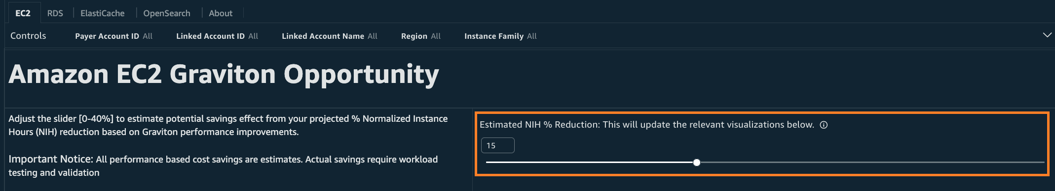
Figure 1: NIH slider location
Assume that your testing shows that your workload runs just as effectively with 15% fewer normalized instance hours on AWS Graviton. You can now plug that exact number into the slider to see your modeled savings combining both pricing differences and compute hour reductions. Although we’ve heard success stories of significant reductions from customers, we recommend starting your initial estimate with a conservative 10% baseline and adjusting based on your own testing results.
Enhanced cost analysis visualizations
The dashboard presents key visualizations that demonstrate the direct relationship between NIH reduction and cost savings. First, you see the Potential Graviton Base Savings from pricing differences alone. In the following diagram, we can observe an example of $61.54K of cost savings from migrating to equivalent AWS Graviton instances. Next, the Estimated Additional Savings Due to Performance in the same diagram shows $42.40K in savings if your performance testing confirms a 15% NIH reduction in your workload. Finally, the dashboard sums these two values into the Total Potential Graviton Savings of $103.94K. The Total Potential Graviton Savings helps visualize how both pricing benefits and any validated compute hour reductions could contribute to your overall savings.
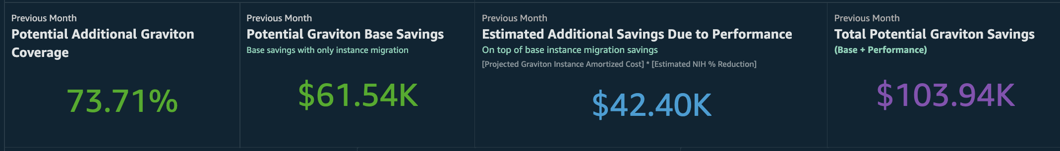
Figure 2: Visualization with relationship between NIH reduction and cost savings
The Amortized Cost Breakdown and Normalized Instance Hrs Breakdown charts in the following figure show 6-month historical trends, helping you spot patterns such as seasonal spikes or high-usage periods. These patterns can help you identify where even small efficiency improvements might yield significant savings, for example, workloads with consistently high usage or predictable peak periods that would be good candidates for testing.
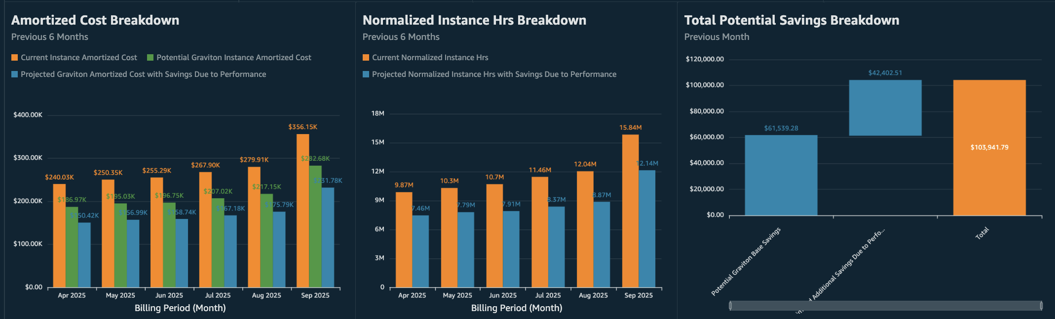
Figure 3: Amortized Cost, NIH, and Total Potential Savings Breakdown charts
Detailed savings analysis
Building on our commitment to help customers optimize cloud costs, we’ve enhanced the Potential Graviton Savings Details table with two columns focused on performance-based savings modeling. The Estimated Additional Savings Due to Performance column shows the modeled savings based on your chosen NIH reduction percentage, while Total Potential Graviton Savings combines this with the base pricing benefits.
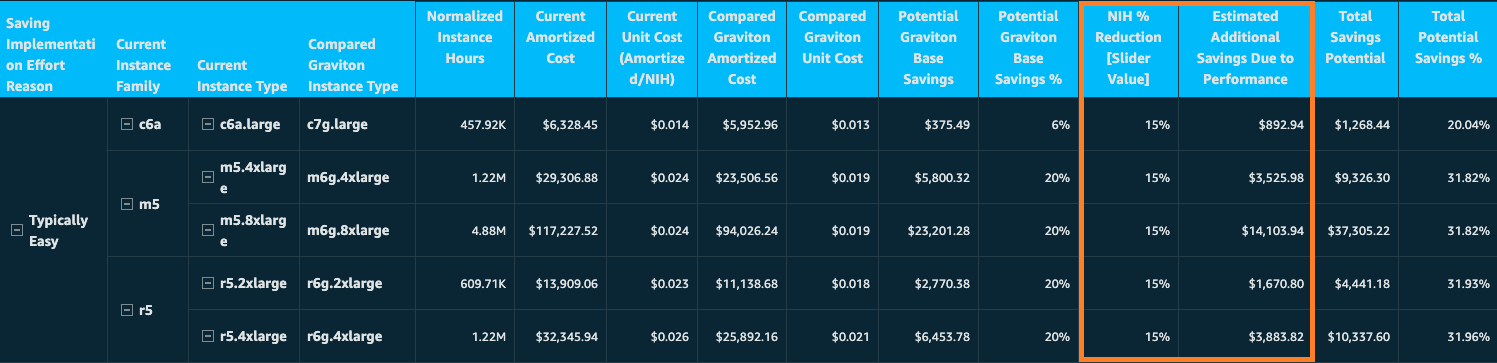
Figure 4: Potential Graviton Savings Details table
As you examine your current instance family, you can observe both baseline AWS Graviton savings and these added saving opportunities clearly laid out in a comprehensive breakdown. The analysis presents your total savings potential in both dollar amounts and percentages. This allows you to build a compelling business case for migration. Although this detailed breakdown provides valuable planning insights, remember that actual savings may vary depending on your specific workload patterns, implementation approaches, and operational considerations.
Conclusion
The Graviton Savings Dashboard (GSD) serves as a powerful analytics tool that streamlines your journey to cost-effective cloud computing. The GSD provides clear visualizations and interactive features to help you understand and maximize potential savings when migrating to AWS Graviton-based instances. To further explore the new features, navigate to the GSD interactive demo, where you can model an example of potential savings using the NIH reduction slider and detailed cost breakdowns.
Ready to explore how AWS Graviton can transform your infrastructure costs? Visit the GSD page to deploy or update your GSD dashboard. Access implementation guides, such as the CFM Technical Implementation Playbook (CFM TIPs), and start optimizing your cloud spend today with the enhanced capabilities of the GSD.
Over 85,000 AWS customers have discovered the benefits of AWS Graviton, with many completing their adoptions in just hours. We have created this resource guide so that you can accelerate your AWS Graviton adoption with minimal effort and enjoy significant price performance benefits.
“What I always tell customers is one week, one application, one engineer, and see what you can do. They always are pleasantly surprised by how much progress they can make. If you’re out there and you haven’t yet moved to AWS Graviton, what are you waiting for? Let’s make it happen!”
Dave Brown, VP, AWS Compute & ML Services
Important note about performance testing
The GSD does not attempt to estimate the potential NIH percent reduction or your workload’s performance when transitioned to AWS Graviton. You can use it to perform what-if analysis of your potential savings for a projected NIH percent reduction. In the absence of this variable, GSD only considers the price delta between instance types and misses an important contributor to the overall savings potential of AWS Graviton from the performance upside. Compute performance is always workload and use case specific, so we encourage you to test your AWS Graviton-based workloads using the Optimization and Performance Runbook to help you determine the actual possible NIH percent reduction.


 Enrique Salgado Hernández is a Senior Specialist Solutions Architect at AWS with more than 10 years of experience working in the cloud. He specializes in designing and implementing large-scale analytics architectures across various industry sectors. He is passionate about working with customers to solve their problems by supporting them during their cloud journey.
 Angel Conde Manjon is a Senior EMEA Data & AI PSA, based in Madrid. He previously worked on research related to data analytics and AI in diverse European research projects. In his current role, Angel helps partners develop businesses centered on data and AI.


 Sandeep Bajwa is a Sr. Analytics Specialist based out of Northern Virginia, specialized in the design and implementation of analytics and data lake solutions.

 Frank Contrepois is the Head of FinOps at
  Aaron Edell is Head of GTM for Customer Cloud Intelligence for Amazon Web Services. He is responsible for building and scaling businesses around Cloud Financial Management, FinOps, and the Well-Architected Cost Optimization pillar. He focuses his GTM efforts on the Cloud Intelligence Dashboards and remains obsessed with helping all customers get better visibility and access to their cost and usage data.


