Tag Archives: Cost Management

Analyze Amazon S3 storage costs using AWS Cost and Usage Reports, Amazon S3 Inventory, and Amazon Athena

Post Syndicated from Dagar Katyal original https://aws.amazon.com/blogs/big-data/analyze-amazon-s3-storage-costs-using-aws-cost-and-usage-reports-amazon-s3-inventory-and-amazon-athena/

Since its launch in 2006, Amazon Simple Storage Service (Amazon S3) has experienced major growth, supporting multiple use cases such as hosting websites, creating data lakes, serving as object storage for consumer applications, storing logs, and archiving data. As the application portfolio grows, customers tend to store data from multiple application and different business functions in a single S3 bucket, which can grow the storage in S3 buckets to hundreds of TBs. The AWS Billing console provides a way to look at the total storage cost of data stored in Amazon S3, but sometimes IT organizations need to understand the breakdown of costs of a particular S3 bucket by various prefixes or objects corresponding to a particular user or application. There are various reasons to analyze the costs of S3 buckets, such as to identify the spend breakdown, do internal chargebacks, understand the cost breakdown by business unit and application, and many more. As of this writing, there is no easy way to do a cost breakdown of S3 buckets by objects and prefixes.

In this post, we discuss a solution using Amazon Athena to query AWS Cost and Usage Reports and Amazon S3 Inventory reports to analyze the cost by prefixes and objects in an S3 bucket.

Overview of solution

The following figure shows the architecture for this solution. First, we enable the AWS Cost and Usage Reports (AWS CUR) and Amazon S3 Inventory features, which save the output into two separate pre-created S3 buckets. We then use Athena to query these S3 buckets for AWS CUR data and S3 object inventory data to correlate and allocate the cost breakdown at the object or prefix level.

architecture diagram

To implement the solution, we complete the following steps:

  1. Create S3 buckets for AWS CUR, S3 object inventory, and Athena results. Alternatively, you can create these respective buckets when enabling the respective individual features, but for the purpose of this post, we create all of them at the beginning.
  2. Enable the Cost and Usage Reports.
  3. Enable Amazon S3 Inventory configuration.
  4. Create AWS Glue Data Catalog tables for the CUR and S3 object inventory to query using Athena.
  5. Run queries in Athena.

Prerequisites

For this walkthrough, you should have the following prerequisites:

Create S3 buckets

Amazon S3 is an object storage service offering industry-leading scalability, data availability, security, and performance. Customers of all sizes and industries can store and protect any amount of data for virtually any use case, such as data lakes, cloud-native applications, and mobile apps. With cost-effective storage classes and easy-to-use management features, you can optimize costs, organize data, and configure fine-tuned access controls to meet specific business, organizational, and compliance requirements.

For this post, we use the S3 bucket s3-object-cost-allocation as the primary bucket for cost allocation. This S3 bucket is conveniently modeled to contain several prefixes and objects of different sizes for which cost allocation needs to be done based on the overall cost of the bucket. In a real-world scenario, you should use a bucket that has data for multiple teams and for which you need to allocate costs by prefix or object. Going forward, we refer to this bucket as the primary object bucket.

The following screenshot shows our S3 bucket and folders.

example Folders created

Now let’s create the three additional operational S3 buckets to store the datasets generated to calculate costs for the objects. You can create the following buckets or any existing buckets as needed:

  • cur-cost-usage-reports-<account_number> – This bucket is used to save the Cost and Usage Reports for the account.
  • S3-inventory-configurations-<account_number> – This bucket is used to save the inventory configurations of our primary object bucket.
  • athena-query-bucket-<account_number> – This bucket is used to save the query results from Athena.

Complete the following steps to create your S3 buckets:

  • On the Amazon S3 console, choose Buckets in the navigation pane.
  • Choose Create bucket.
  • For Bucket name, enter the name of your bucket (cur-cost-usage-reports-<account_number>).
  • For AWS Region, choose your preferred Region.
  • Leave all other settings at default (or according to your organization’s standards).
  • Choose Create bucket.
    create s3 bucket
  • Repeat these steps to create s3-inventory-configurations-<account_number> and athena-query-bucket-<account_number>.

Enable the Cost and Usage Reports

The AWS Cost and Usage Reports (AWS CUR) contains the most comprehensive set of cost and usage data available. You can use Cost and Usage Reports to publish your AWS billing reports to an S3 bucket that you own. You can receive reports that break down your costs by the hour, day, or month; by product or product resource; or by tags that you define yourself.

Complete the following steps to enable Cost and Usage Reports for your account:

  • On the AWS Billing console, in the navigation pane, choose Cost & Usage Reports.
  • Choose Create report.
  • For Report name, enter a name for your report, such as account-cur-s3.
  • For Additional report details, select Include resource IDs to include the IDs of each individual resource in the report.Including resource IDs will create individual line items for each of your resources. This can increase the size of your Cost and Usage Reports files significantly, which can affect the S3 storage costs for your CUR, based on your AWS usage. We need this feature enabled for this post.
  • For Data refresh settings, select whether you want the Cost and Usage Reports to refresh if AWS applies refunds, credits, or support fees to your account after finalizing your bill.When a report refreshes, a new report is uploaded to Amazon S3.
  • Choose Next.
  • For S3 bucket, choose Configure.
  • For Configure S3 Bucket, select an existing bucket created in the previous section (cur-cost-usage-reports-<account_number>) and choose Next.
  • Review the bucket policy, select I have confirmed that this policy is correct, and choose Save. This default bucket policy provides Cost and Usage Reports access to write data to Amazon S3.
  • For Report path prefix, enter cur-data/account-cur-daily.
  • For Time granularity, choose Daily.
  • For Report versioning, choose Overwrite existing report.
  • For Enable report data integration for, select Amazon Athena.
  • Choose Next.
  • After you have reviewed the settings for your report, choose Review and Complete.
    create cost and usage report

The Cost and Usage reports will be delivered to the S3 buckets within 24 hours.

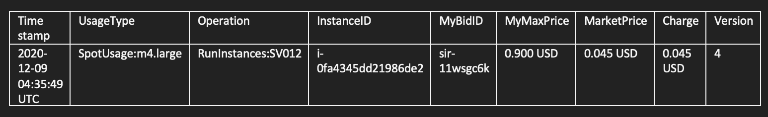
The following sample CUR in CSV format shows different columns of the Cost and Usage Report, including bill_invoice_id, bill_invoicing_entity, bill_payer_account_id, and line_item_product_code, to name a few.

sample cost and usage report

Enable Amazon S3 Inventory configuration

Amazon S3 Inventory is one of the tools Amazon S3 provides to help manage your storage. You can use it to audit and report on the replication and encryption status of your objects for business, compliance, and regulatory needs. Amazon S3 Inventory provides comma-separated values (CSV), Apache Optimized Row Columnar (ORC), or Apache Parquet output files that list your objects and their corresponding metadata on a daily or weekly basis for an S3 bucket or a shared prefix (objects that have names that begin with a common string).

Complete the following steps to enable Amazon S3 Inventory on the primary object bucket:

  • On the Amazon S3 console, choose Buckets in the navigation pane.
  • Choose the bucket for which you want to configure Amazon S3 Inventory.
    This will be the existing bucket in your account that has data that needs to be analyzed. This could be your data lake or application S3 bucket. We created the bucket s3-object-cost-allocation with some sample data and folder structure.
  • Choose Management.
  • Under Inventory configurations, choose Create inventory configuration.
  • For Inventory configuration name, enter s3-object-cost-allocation.
  • For Inventory scope, leave Prefix blank.
    This is to ensure that all objects are covered for the report.
  • For Object Versions, select Current version only.
  • For Report details, choose This account.
  • For Destination, choose the destination bucket we created (s3-inventory-configurations-<account_number>).
  • For Frequency, choose Daily.
  • For Output format, choose as Apache Parquet.
  • For Status, choose Enable.
  • Keep server-side encryption disabled. To use server-side encryption, choose Enable and specify the encryption key.
  • For Additional fields, select the following to add to the inventory report:
    • Size – The object size in bytes.
    • Last modified date – The object creation date or the last modified date, whichever is the latest.
    • Multipart upload – Specifies that the object was uploaded as a multipart upload. For more information, see Uploading and copying objects using multipart upload.
    • Replication status – The replication status of the object. For more information, see Using the S3 console.
    • Encryption status – The server-side encryption used to encrypt the object. For more information, see Protecting data using server-side encryption.
    • Bucket key status – Indicates whether a bucket-level key generated by AWS KMS applies to the object.
    • Storage class – The storage class used for storing the object.
    • Intelligent-Tiering: Access tier – Indicates the access tier of the object if it was stored in Intelligent-Tie
      create s3 inventory
  • Choose Create.
    s3 inventory configuration

It may take up to 48 hours to deliver the first report.

Create AWS Glue Data Catalog tables for CUR and Amazon S3 Inventory reports

Wait for up to 48 hours for the previous step to generate the reports. In this section, we use Athena to create and define AWS Glue Data Catalog tables for the data that has been created using Cost and Usage Reports and Amazon S3 Inventory reports.

Athena is a serverless, interactive analytics service built on open-source frameworks, supporting open-table and file formats. Athena provides a simplified, flexible way to analyze petabytes of data where it lives.

Complete the following steps to create the tables using Athena:

  • Navigate to the Athena console.
  • If you’re using Athena for the first time, you need to set up a query result location in Amazon S3. If you preconfigured this in Athena , you can skip this step.
    • Choose View settings.
      athena setup query bucket
    • Choose Manage.
    • In the section Query result location and encryption, choose Browse S3 and choose the bucket that we created (athena-query-bucket-<account_number>).
    • Choose Save.
      Athena Config
    • Navigate back to the Athena query editor.
  • Run the following query in Athena to create a table for Cost and Usage Reports. Verify and update the section for <<LOCATION>> at the end of the query and point it to the correct S3 bucket and location. Note that the new table name should be account_cur.
    CREATE EXTERNAL TABLE `account_cur`(
    `identity_line_item_id` string,
    `identity_time_interval` string,
    `bill_invoice_id` string,
    `bill_billing_entity` string,
    `bill_bill_type` string,
    `bill_payer_account_id` string,
    `bill_billing_period_start_date` timestamp,
    `bill_billing_period_end_date` timestamp,
    `line_item_usage_account_id` string,
    `line_item_line_item_type` string,
    `line_item_usage_start_date` timestamp,
    `line_item_usage_end_date` timestamp,
    `line_item_product_code` string,
    `line_item_usage_type` string,
    `line_item_operation` string,
    `line_item_availability_zone` string,
    `line_item_resource_id` string,
    `line_item_usage_amount` double,
    `line_item_normalization_factor` double,
    `line_item_normalized_usage_amount` double,
    `line_item_currency_code` string,
    `line_item_unblended_rate` string,
    `line_item_unblended_cost` double,
    `line_item_blended_rate` string,
    `line_item_blended_cost` double,
    `line_item_line_item_description` string,
    `line_item_tax_type` string,
    `line_item_legal_entity` string,
    `product_product_name` string,
    `product_availability` string,
    `product_description` string,
    `product_durability` string,
    `product_event_type` string,
    `product_fee_code` string,
    `product_fee_description` string,
    `product_free_query_types` string,
    `product_from_location` string,
    `product_from_location_type` string,
    `product_from_region_code` string,
    `product_group` string,
    `product_group_description` string,
    `product_location` string,
    `product_location_type` string,
    `product_message_delivery_frequency` string,
    `product_message_delivery_order` string,
    `product_operation` string,
    `product_platopricingtype` string,
    `product_product_family` string,
    `product_queue_type` string,
    `product_region` string,
    `product_region_code` string,
    `product_servicecode` string,
    `product_servicename` string,
    `product_sku` string,
    `product_storage_class` string,
    `product_storage_media` string,
    `product_to_location` string,
    `product_to_location_type` string,
    `product_to_region_code` string,
    `product_transfer_type` string,
    `product_usagetype` string,
    `product_version` string,
    `product_volume_type` string,
    `pricing_rate_code` string,
    `pricing_rate_id` string,
    `pricing_currency` string,
    `pricing_public_on_demand_cost` double,
    `pricing_public_on_demand_rate` string,
    `pricing_term` string,
    `pricing_unit` string,
    `reservation_amortized_upfront_cost_for_usage` double,
    `reservation_amortized_upfront_fee_for_billing_period` double,
    `reservation_effective_cost` double,
    `reservation_end_time` string,
    `reservation_modification_status` string,
    `reservation_normalized_units_per_reservation` string,
    `reservation_number_of_reservations` string,
    `reservation_recurring_fee_for_usage` double,
    `reservation_start_time` string,
    `reservation_subscription_id` string,
    `reservation_total_reserved_normalized_units` string,
    `reservation_total_reserved_units` string,
    `reservation_units_per_reservation` string,
    `reservation_unused_amortized_upfront_fee_for_billing_period` double,
    `reservation_unused_normalized_unit_quantity` double,
    `reservation_unused_quantity` double,
    `reservation_unused_recurring_fee` double,
    `reservation_upfront_value` double,
    `savings_plan_total_commitment_to_date` double,
    `savings_plan_savings_plan_a_r_n` string,
    `savings_plan_savings_plan_rate` double,
    `savings_plan_used_commitment` double,
    `savings_plan_savings_plan_effective_cost` double,
    `savings_plan_amortized_upfront_commitment_for_billing_period` double,
    `savings_plan_recurring_commitment_for_billing_period` double,
    `resource_tags_user_bucket_name` string,
    `resource_tags_user_cost_tracking` string)
    PARTITIONED BY (
    `year` string,
    `month` string)
    ROW FORMAT SERDE
    'org.apache.hadoop.hive.ql.io.parquet.serde.ParquetHiveSerDe'
    STORED AS INPUTFORMAT
    'org.apache.hadoop.mapred.TextInputFormat'
    OUTPUTFORMAT
    'org.apache.hadoop.hive.ql.io.HiveIgnoreKeyTextOutputFormat'
    LOCATION
    '<<LOCATION>>'
  • Run the following query in Athena to create the table for Amazon S3 Inventory. Verify and update the section for <<LOCATION>> at the end of the query and point it to the correct S3 bucket and location.
    • To get the exact value of the location, navigate to the bucket where inventory configurations are stored and navigate to the folder path Hive . Use the S3 URI to replace <<LOCATION>> in the query.query path location
      CREATE EXTERNAL TABLE s3_object_inventory(
               bucket string,
               key string,
               version_id string,
               is_latest boolean,
               is_delete_marker boolean,
               size bigint,
               last_modified_date bigint,
               storage_class string,
               is_multipart_uploaded boolean,
               replication_status string,
               encryption_status string,
               intelligent_tiering_access_tier string,
               bucket_key_status string
      ) PARTITIONED BY (
              dt string
      )
      ROW FORMAT SERDE 'org.apache.hadoop.hive.ql.io.parquet.serde.ParquetHiveSerDe'
        STORED AS INPUTFORMAT 'org.apache.hadoop.hive.ql.io.SymlinkTextInputFormat'
        OUTPUTFORMAT 'org.apache.hadoop.hive.ql.io.IgnoreKeyTextOutputFormat'
        LOCATION '<<LOCATION>>';
      
  • We need to refresh the partitions and add new inventory lists to the table. Use the following commands to add data to the CUR table and Amazon S3 Inventory table:
    MSCK REPAIR TABLE `account_cur`;
    
    MSCK REPAIR TABLE s3_object_inventory;

Run queries in Athena to allocate the cost of objects in an S3 bucket

Now we can query the data we have available to get a cost allocation breakdown at the prefix level.

We need to provide some information in the following queries:

  • Update <<YYYY-MM-DD>> with the date for which you want to analyze the data
  • Update <<prefix>> with the prefix values for your bucket that needs to be analyzed
  • Update <<bucket_name>> with the name of the bucket that needs to be analyzed

We use the following part of the query to calculate the size of storage being used by the target prefix that we want to calculate the cost for:

select date_parse(dt,'%Y-%m-%d-%H-%i') dt, cast (sum(size) as double) targetPrefixBytes
from s3_object_inventory
where date_parse(dt,'%Y-%m-%d-%H-%i') = cast('<<YYYY-MM-DD>>' as timestamp)
and key like '<<prefix>>/%'
group by dt

Next, we calculate the total size of the bucket on that particular date:

select date_parse(dt,'%Y-%m-%d-%H-%i') dt, cast (sum(size) as double) totalBytes
from s3_object_inventory
where date_parse(dt,'%Y-%m-%d-%H-%i') = cast('<<YYYY-MM-DD>>' as timestamp)
group by dt

We query the CUR table to get the cost of a particular bucket on a particular date:

select line_item_usage_start_date as dt, sum(line_item_blended_cost) as line_item_blended_cost
from "account_cur"
where line_item_product_code = 'AmazonS3'
and product_servicecode = 'AmazonS3'
and line_item_operation = 'StandardStorage'
and line_item_resource_id = '<<bucket_name>>'
and line_item_usage_start_date = cast('<<YYYY-MM-DD>>' as timestamp)
group by line_item_usage_start_date

Putting all of this together, we can calculate the cost of a particular prefix (folder or a file) on a specific date. The complete query is as follows:

with
cost as (select line_item_usage_start_date as dt, sum(line_item_blended_cost) as line_item_blended_cost
from "account_cur"
where line_item_product_code = 'AmazonS3'
and product_servicecode = 'AmazonS3'
and line_item_operation = 'StandardStorage'
and line_item_resource_id = '<<bucket_name>>'
and line_item_usage_start_date = cast('<<YYYY-MM-DD>>' as timestamp)
group by line_item_usage_start_date),
total as (select date_parse(dt,'%Y-%m-%d-%H-%i') dt, cast (sum(size) as double) totalBytes
from s3_object_inventory
where date_parse(dt,'%Y-%m-%d-%H-%i') = cast('<<YYYY-MM-DD>>' as timestamp)
group by dt),
target as (select date_parse(dt,'%Y-%m-%d-%H-%i') dt, cast (sum(size) as double) targetPrefixBytes
from s3_object_inventory
where date_parse(dt,'%Y-%m-%d-%H-%i') = cast('<<YYYY-MM-DD>>' as timestamp)
and key like '<<prefix>>/%'
group by dt)
select target.dt,
(target.targetPrefixBytes/ total.totalBytes * 100) percentUsed,
cost.line_item_blended_cost totalCost,
cost.line_item_blended_cost*(target.targetPrefixBytes/ total.totalBytes) as prefixCost
from target, total, cost
where target.dt = total.dt
and target.dt = cost.dt

The following screenshot shows the results table for the sample data we used in this post. We get the following information:

  • dt – Date
  • percentUsed – The percentage of prefix space compared to overall bucket space
  • totalCost – The total cost of the bucket
  • prefixCost – The cost of the space used by the prefix

final result percetage

Clean up

To stop incurring costs, be sure to disable Amazon S3 Inventory and Cost and Usage Reports when you’re done.

Delete the S3 buckets created for the Amazon S3 Inventory reports and Cost and Usage Reports to avoid storage charges.

Other methods for Amazon S3 storage analysis

Amazon S3 Storage Lens can provide a single view of object storage usage and activity across your entire Amazon S3 storage. With S3 Storage Lens, you can understand, analyze, and optimize storage with over 29 usage and activity metrics and interactive dashboards to aggregate data for your entire organization, specific accounts, Regions, buckets, or prefixes. All of this data is accessible on the Amazon S3 console or as raw data in an S3 bucket.

S3 Storage Lens doesn’t provide cost analysis based on an object or prefix in a single bucket. If you want visibility of storage usage and trends across the entire storage footprint along with recommendations on cost efficiency and data protection best practices, S3 Storage Lens is the right option. But if you want a cost analysis of specific S3 buckets and looking for ways to get cost allocation of S3 objects at the object or prefix level, the solution in this post would be the best fit.

Conclusion

In this post, we detailed how to create a cost breakdown model at the object or prefix level for S3 buckets that contains data for multiple business units and applications. We used Athena to query the reports and datasets produced by the AWS CUR and Amazon S3 Inventory features that, when correlated, give us the cost allocation at the object and prefix level. This solution gives you an easy way to calculate costs for independent objects and prefixes, which can be used for internal chargebacks or just to know the per-object or per-prefix spending in a shared S3 bucket.


About the Authors


Dagar Katyal
is a Senior Solutions Architect at AWS, based in Chicago, Illinois. He works with customers and provides guidance for key strategic initiatives important for their business. Dagar has an MBA and has spent years over 15 years working with customers on projects on analytics strategy, roadmap, and using data as a key differentiator. When not working with customers, Dagar spends time with his family and doing home improvement projects.


Saiteja Pudi
is a Solutions Architect at AWS, based in Dallas, Tx. He has been with AWS for more than 3 years now, helping customers derive the true potential of AWS by being their trusted advisor. He comes from an application development background, interested in Data Science and Machine Learning.

Diving Deep into EC2 Spot Instance Cost and Operational Practices

Post Syndicated from Sheila Busser original https://aws.amazon.com/blogs/compute/diving-deep-into-ec2-spot-instance-cost-and-operational-practices/

This blog post is written by, Sudhi Bhat, Senior Specialist SA, Flexible Compute.

Amazon EC2 Spot Instances are one of the popular choices among customers looking to cost optimize their workload running on AWS. Spot Instances let you take advantage of unused Amazon Elastic Compute Cloud (Amazon EC2) capacity in the AWS cloud and are available at up to a 90% discount compared to On-Demand EC2 instance prices. The key difference between On-Demand Instances and Spot Instances is that Spot Instances can be interrupted by Amazon EC2, with two minutes of notification, when Amazon EC2 needs the capacity back. Spot Instances are recommended for various stateless, fault-tolerant, or flexible applications, such as big data, containerized workloads, continuous integration/continuous development (CI/CD), web servers, high-performance computing (HPC), and test and development workloads.

Customers asked us for fast and easy ways to track and optimize usage for different services. In this post, we’ll focus on tools and techniques that can provide useful insights into the usages and behavior of workloads using Spot Instances, as well as how we can leverage those techniques for troubleshooting and cost tracking purposes.

Operational tools

Instance selection

One of the best practices while using Spot Instances is to be flexible about instance types, Regions, and Availability Zones, as this gives Spot a better cross-section of compute pools to select and allocate your desired capacity. AWS makes it easier to diversify your instance selection in Auto Scaling groups and EC2 Fleet through features like Attribute-Based Instance Type Selection, where you can select the instance requirements as a set of attributes like vCPU, memory, storage, etc. These requirements are translated into matching instance types automatically.

Instance Selection using Attribute Based Instance Selection feature available during Auto Scaling Group creation

Considering that AWS Cloud spans across 25+ Regions and 80+ Availability Zones, finding the optimal location (either a Region or Availability Zone) to fulfil Spot capacity needs without launching a Spot can be very handy. This is especially true when AWS customers have the flexibility to run their workloads across multiple Regions or Availability Zones. This functionality can be achieved with one of the newer features called Amazon EC2 Spot placement score. Spot placement score provides a list of Regions or Availability Zones, each scored from 1 to 10, based on factors such as the requested instance types, target capacity, historical and current Spot usage trends, and the time of the request. The score reflects the likelihood of success when provisioning Spot capacity, with a 10 meaning that the request is highly likely to succeed.

Spot Placement Score feature is available in EC2 Dashboard

If you wish to specifically select and match your instances to your workloads to leverage them, then refer to Spot Instance Advisor to determine Spot Instances that meet your computing requirements with their relative discounts and associated interruption rates. Spot Instance Advisor populates the frequency of interruption and average savings over On-Demand instances based on the last 30 days of historical data. However, note that the past interruption behavior doesn’t predict the future availability of these instances. Therefore, as a part of instance diversity, try to leverage as many instances as possible regardless of whether or not an instance has a high level of interruptions.

Spot Instance pricing history

Understanding the price history for a specific Amazon EC2 Spot Instance can be useful during instance selection. However, tracking these pricing changes can be complex. Since November 2017, AWS launched a new pricing model that simplified the Spot purchasing experience. The new model gives AWS Customers predictable prices that adjust slowly over days and weeks, as Spot Instance prices are now determined based on long-term trends in supply and demand for Spot Instance capacity. The current Spot Instance prices can be viewed on AWS website, and the Spot Instance pricing history can be viewed on the Amazon EC2 console or accessed via AWS Command Line Interface (AWS CLI). Customers can continue to access the Spot price history for the last 90 days, filtering by instance type, operating system, and Availability Zone to understand how the Spot pricing has changed.

Spot Pricing History is available in EC2 DashboardAccessing Pricing history via AWS CLI using describe-spot-price-history or Get-EC2SpotPriceHistory (AWS Tools for Windows PowerShell).

aws ec2 describe-spot-price-history --start-time 2018-05-06T07:08:09 --end-time 2018-05-06T08:08:09 --instance-types c4.2xlarge --availability-zone eu-west-1a --product-description "Linux/UNIX (Amazon VPC)“
{
    "SpotPriceHistory": [
        {
            "Timestamp": "2018-05-06T06:30:30.000Z",
            "AvailabilityZone": "eu-west-1a",
            "InstanceType": "c4.2xlarge",
            "ProductDescription": "Linux/UNIX (Amazon VPC)",
            "SpotPrice": "0.122300"
        }
    ]
}

Spot Instance data feed

EC2 offers a mechanism to describe Spot Instance usage and pricing by providing a data feed that can be subscribed to. Therefore, the data feed is sent to an Amazon Simple Storage Service (Amazon S3) bucket on an hourly basis. Learn more about setting up the Spot Data feed and configuring the S3 bucket options in the documentation. A sample data feed would look like the following:

Sample Spot Instance data feed dataThe above example provides more information about Spot Instance in use, like m4.large Instance being used at the time as specified by Timestamp and MyBidID=sir-11wsgc6k representing the request that generated this instance usage, Charge=0.045 USD indicating the discounted price charged compared to the MyMaxPrice, which was set to On-Demand cost. This information can be useful during troubleshooting, as you can refer to the information about Spot Instances even if that specific instance has been terminated. Moreover, you could choose to extend the use of this data for simple querying and visualization/analytics purposes using Amazon Athena.

Amazon EC2 Spot Instance Interruption dashboard

Spot Instance interruptions are an inherent part of the Spot Instance lifecycle. For example, it’s always possible that your Spot Instance might be interrupted depending on how many unused EC2 instances are available. Therefore, you must make sure that your application is prepared for a Spot Instance interruption.

There are several best practices regarding handling Spot interruptions as described in the blog “Best practices for handling EC2 Spot Instance interruptions. Tracking Spot Instance interruptions can be useful in some scenarios, such as evaluating your workload for the tolerance for interruptions of a specific instance type, or to simply learn more about frequency of interruptions in your test environment so that you can fine-tune your instance selection. In these scenarios, you can use the EC2 Spot interruption dashboard, which is an opensource sample reference solution for logging Spot Instance interruptions. Spot Instance interruptions can fluctuate dynamically based on overall Spot Instance availability and demand for On-Demand Instances. However, it is important to note that tracking interruptions may not always represent the true Spot experience. Therefore, it’s recommended that this solution be used for those situations where Spot Instance interruptions inform a specific outcome, as it doesn’t accurately reflect system health or availability. It’s recommended to use this solution in dev/test environments to provide an educated view of how to use Spot Instances in production systems.

Open Source Solution available in github called Spot Interruption Dashboard for tracking Spot Interruption termination notices.

Cost management tools

AWS Pricing Calculator

AWS Pricing Calculator is a free tool that lets you create cost estimates for workloads that you run on AWS Services, including EC2 and Spot Instances. This calculator can greatly assist in calculating the cost of compute instances and estimating the future costs so that customers can compare the cost savings to be achieved before they even launch a Spot Instance as part of their solution. The AWS Pricing Calculator advanced estimate path offers six pricing strategies for Amazon EC2 instances. The pricing models include On-Demand, Reserved, Savings Plans, and Spot Instances. The estimates generated can also be exported to a CSV or PDF file format for quick sharing and additional analysis of the proposed architecture spend.

AWS Pricing Calculator support different types of workloadsFor Spot Instances, the calculator shows the historical average discount percentage for the instance chosen, and lets you enter a percentage discount for creating forecasts. We recommend choosing an instance type that best represents your target compute, memory, and network requirements for running your workload and generating an approximate estimate.

AWS Pricing Calculator Supports different type of EC2 Purchasing options, including EC2 Spot instances

AWS Cost Management

One of the popular reporting tools offered by AWS is AWS Cost Explorer, which has an easy-to-use interface that lets you visualize, understand, and manage your AWS costs and usage over time, including Spot Instances. You can view data up to the last 12 months, and forecast the next three months. You can use Cost Explorer filtered by “Purchase Options” to see patterns in how much you spend on Spot Instances over time, and see trends that you can use to understand your costs. Furthermore, you can specify time ranges for the data, and view time data by day or by month. Moreover, you can leverage the Amazon EC2 Instance Usage reports to gain insights into your instance usage and patterns, along with information that you need to optimize the overall EC2 use.

AWS Cost Explores shows cost incurred in multiple different compute purchasing options

AWS Billing and Cost Management offers a way to organize your resource costs on your cost allocation report by leveraging cost allocation tags, so that it’s easier to categorize and track your AWS costs using cost allocation reports, which includes all of your AWS costs for each billing period. The report includes both tagged and untagged resources, so that you can clearly organize the charges for resources. For example, if you tag resources with an application name that is deployed on Spot Instances, you can track the total cost of that single application that runs on those resources. The AWS generated tags “createdBy” is a tag that AWS defines and applies to supported AWS resources for cost allocation purposes and if opted, this tag is applied to “Spot-instance-request” resource type whenever the RequestSpotInstances API is invoked. This can be a great way to track the Spot Instance creation activities in your billing reports.

Cost and Usage Reports

AWS Customers have access to raw cost and usage data through the AWS Cost and Usage (AWS CUR) reports. These reports contain the most comprehensive information about your AWS usage and costs. Financial teams need this data so that they have an overview of their monthly, quarterly, and yearly AWS spend. But this data is equally valuable for technical teams who need detailed resource-level granularity to understand which resources are contributing to the spend, and what parts of the system to optimize. If you’re using Spot Instances for your compute needs, then AWS CUR populates the Amazon EC2 Spot usage pricing/* columns and the product/* columns. With this data, you can calculate the past savings achieved with Spot through the AWS CUR. Note that this feature was enabled in July 2021 and the AWS CUR data for Spot Usage is available only since then. The Cloud Intelligence Dashboards provide prebuilt visualizations that can help you get a detailed view of your AWS usage and costs. You can learn more about deploying Cloud Intelligence Dashboards by referring to the detailed blog “Visualize and gain insight into you AWS cost and usage with Cloud Intelligence Dashboard and CUDOS using Amazon QuickSite”Compute summary can be viewed in Cloud Intelligent Dashboards

Conclusion

It’s always recommended to follow Spot Instance best practices while using Amazon EC2 Spot Instances for suitable workloads, so that you can have the best experience. In this post, we explored a few tools and techniques that can further guide you toward much deeper insights into your workloads that are using Spot Instances. This can assist you with understanding cost savings and help you with troubleshooting so that you can use Spot Instances more easily.

Optimizing AWS Lambda cost and performance using AWS Compute Optimizer

Post Syndicated from Chad Schmutzer original https://aws.amazon.com/blogs/compute/optimizing-aws-lambda-cost-and-performance-using-aws-compute-optimizer/

This post is authored by Brooke Chen, Senior Product Manager for AWS Compute Optimizer, Letian Feng, Principal Product Manager for AWS Compute Optimizer, and Chad Schmutzer, Principal Developer Advocate for Amazon EC2

Optimizing compute resources is a critical component of any application architecture. Over-provisioning compute can lead to unnecessary infrastructure costs, while under-provisioning compute can lead to poor application performance.

Launched in December 2019, AWS Compute Optimizer is a recommendation service for optimizing the cost and performance of AWS compute resources. It generates actionable optimization recommendations tailored to your specific workloads. Over the last year, thousands of AWS customers reduced compute costs up to 25% by using Compute Optimizer to help choose the optimal Amazon EC2 instance types for their workloads.

One of the most frequent requests from customers is for AWS Lambda recommendations in Compute Optimizer. Today, we announce that Compute Optimizer now supports memory size recommendations for Lambda functions. This allows you to reduce costs and increase performance for your Lambda-based serverless workloads. To get started, opt in for Compute Optimizer to start finding recommendations.

Overview

With Lambda, there are no servers to manage, it scales automatically, and you only pay for what you use. However, choosing the right memory size settings for a Lambda function is still an important task. Computer Optimizer uses machine-learning based memory recommendations to help with this task.

These recommendations are available through the Compute Optimizer console, AWS CLI, AWS SDK, and the Lambda console. Compute Optimizer continuously monitors Lambda functions, using historical performance metrics to improve recommendations over time. In this blog post, we walk through an example to show how to use this feature.

Using Compute Optimizer for Lambda

This tutorial uses the AWS CLI v2 and the AWS Management Console.

In this tutorial, we setup two compute jobs that run every minute in AWS Region US East (N. Virginia). One job is more CPU intensive than the other. Initial tests show that the invocation times for both jobs typically last for less than 60 seconds. The goal is to either reduce cost without much increase in duration, or reduce the duration in a cost-efficient manner.

Based on these requirements, a serverless solution can help with this task. Amazon EventBridge can schedule the Lambda functions using rules. To ensure that the functions are optimized for cost and performance, you can use the memory recommendation support in Compute Optimizer.

In your AWS account, opt in to Compute Optimizer to start analyzing AWS resources. Ensure you have the appropriate IAM permissions configured – follow these steps for guidance. If you prefer to use the console to opt in, follow these steps. To opt in, enter the following command in a terminal window:

$ aws compute-optimizer update-enrollment-status --status Active

Once you enable Compute Optimizer, it starts to scan for functions that have been invoked for at least 50 times over the trailing 14 days. The next section shows two example scheduled Lambda functions for analysis.

Example Lambda functions

The code for the non-CPU intensive job is below. A Lambda function named lambda-recommendation-test-sleep is created with memory size configured as 1024 MB. An EventBridge rule is created to trigger the function on a recurring 1-minute schedule:

import json
import time

def lambda_handler(event, context):
  time.sleep(30)
  x=[0]*100000000
  return {
    'statusCode': 200,
    'body': json.dumps('Hello World!')
  }

The code for the CPU intensive job is below. A Lambda function named lambda-recommendation-test-busy is created with memory size configured as 128 MB. An EventBridge rule is created to trigger the function on a recurring 1-minute schedule:

import json
import random

def lambda_handler(event, context):
  random.seed(1)
  x=0
  for i in range(0, 20000000):
    x+=random.random()

  return {
    'statusCode': 200,
    'body': json.dumps('Sum:' + str(x))
  }

Understanding the Compute Optimizer recommendations

Compute Optimizer needs a history of at least 50 invocations of a Lambda function over the trailing 14 days to deliver recommendations. Recommendations are created by analyzing function metadata such as memory size, timeout, and runtime, in addition to CloudWatch metrics such as number of invocations, duration, error count, and success rate.

Compute Optimizer will gather the necessary information to provide memory recommendations for Lambda functions, and make them available within 48 hours. Afterwards, these recommendations will be refreshed daily.

These are recent invocations for the non-CPU intensive function:

Recent invocations for the non-CPU intensive function

Function duration is approximately 31.3 seconds with a memory setting of 1024 MB, resulting in a duration cost of about $0.00052 per invocation. Here are the recommendations for this function in the Compute Optimizer console:

Recommendations for this function in the Compute Optimizer console

The function is Not optimized with a reason of Memory over-provisioned. You can also fetch the same recommendation information via the CLI:

$ aws compute-optimizer \
  get-lambda-function-recommendations \
  --function-arns arn:aws:lambda:us-east-1:123456789012:function:lambda-recommendation-test-sleep
{
    "lambdaFunctionRecommendations": [
        {
            "utilizationMetrics": [
                {
                    "name": "Duration",
                    "value": 31333.63587049883,
                    "statistic": "Average"
                },
                {
                    "name": "Duration",
                    "value": 32522.04,
                    "statistic": "Maximum"
                },
                {
                    "name": "Memory",
                    "value": 817.67049838188,
                    "statistic": "Average"
                },
                {
                    "name": "Memory",
                    "value": 819.0,
                    "statistic": "Maximum"
                }
            ],
            "currentMemorySize": 1024,
            "lastRefreshTimestamp": 1608735952.385,
            "numberOfInvocations": 3090,
            "functionArn": "arn:aws:lambda:us-east-1:123456789012:function:lambda-recommendation-test-sleep:$LATEST",
            "memorySizeRecommendationOptions": [
                {
                    "projectedUtilizationMetrics": [
                        {
                            "name": "Duration",
                            "value": 30015.113193697029,
                            "statistic": "LowerBound"
                        },
                        {
                            "name": "Duration",
                            "value": 31515.86878891883,
                            "statistic": "Expected"
                        },
                        {
                            "name": "Duration",
                            "value": 33091.662123300975,
                            "statistic": "UpperBound"
                        }
                    ],
                    "memorySize": 900,
                    "rank": 1
                }
            ],
            "functionVersion": "$LATEST",
            "finding": "NotOptimized",
            "findingReasonCodes": [
                "MemoryOverprovisioned"
            ],
            "lookbackPeriodInDays": 14.0,
            "accountId": "123456789012"
        }
    ]
}

The Compute Optimizer recommendation contains useful information about the function. Most importantly, it has determined that the function is over-provisioned for memory. The attribute findingReasonCodes shows the value MemoryOverprovisioned. In memorySizeRecommendationOptions, Compute Optimizer has found that using a memory size of 900 MB results in an expected invocation duration of approximately 31.5 seconds.

For non-CPU intensive jobs, reducing the memory setting of the function often doesn’t have a negative impact on function duration. The recommendation confirms that you can reduce the memory size from 1024 MB to 900 MB, saving cost without significantly impacting duration. The new duration cost per invocation saves approximately 12%.

The Compute Optimizer console validates these calculations:

Compute Optimizer console validates these calculations

These are recent invocations for the second function which is CPU-intensive:

Recent invocations for the second function which is CPU-intensive

The function duration is about 37.5 seconds with a memory setting of 128 MB, resulting in a duration cost of about $0.000078 per invocation. The recommendations for this function appear in the Compute Optimizer console:

recommendations for this function appear in the Compute Optimizer console

The function is also Not optimized with a reason of Memory under-provisioned. The same recommendation information is available via the CLI:

$ aws compute-optimizer \
  get-lambda-function-recommendations \
  --function-arns arn:aws:lambda:us-east-1:123456789012:function:lambda-recommendation-test-busy
{
    "lambdaFunctionRecommendations": [
        {
            "utilizationMetrics": [
                {
                    "name": "Duration",
                    "value": 36006.85851551957,
                    "statistic": "Average"
                },
                {
                    "name": "Duration",
                    "value": 38540.43,
                    "statistic": "Maximum"
                },
                {
                    "name": "Memory",
                    "value": 53.75978407557355,
                    "statistic": "Average"
                },
                {
                    "name": "Memory",
                    "value": 55.0,
                    "statistic": "Maximum"
                }
            ],
            "currentMemorySize": 128,
            "lastRefreshTimestamp": 1608725151.752,
            "numberOfInvocations": 741,
            "functionArn": "arn:aws:lambda:us-east-1:123456789012:function:lambda-recommendation-test-busy:$LATEST",
            "memorySizeRecommendationOptions": [
                {
                    "projectedUtilizationMetrics": [
                        {
                            "name": "Duration",
                            "value": 27340.37604781184,
                            "statistic": "LowerBound"
                        },
                        {
                            "name": "Duration",
                            "value": 28707.394850202432,
                            "statistic": "Expected"
                        },
                        {
                            "name": "Duration",
                            "value": 30142.764592712556,
                            "statistic": "UpperBound"
                        }
                    ],
                    "memorySize": 160,
                    "rank": 1
                }
            ],
            "functionVersion": "$LATEST",
            "finding": "NotOptimized",
            "findingReasonCodes": [
                "MemoryUnderprovisioned"
            ],
            "lookbackPeriodInDays": 14.0,
            "accountId": "123456789012"
        }
    ]
}

For this function, Compute Optimizer has determined that the function’s memory is under-provisioned. The value of findingReasonCodes is MemoryUnderprovisioned. The recommendation is to increase the memory from 128 MB to 160 MB.

This recommendation may seem counter-intuitive, since the function only uses 55 MB of memory per invocation. However, Lambda allocates CPU and other resources linearly in proportion to the amount of memory configured. This means that increasing the memory allocation to 160 MB also reduces the expected duration to around 28.7 seconds. This is because a CPU-intensive task also benefits from the increased CPU performance that comes with the additional memory.

After applying this recommendation, the new expected duration cost per invocation is approximately $0.000075. This means that for almost no change in duration cost, the job latency is reduced from 37.5 seconds to 28.7 seconds.

The Compute Optimizer console validates these calculations:

Compute Optimizer console validates these calculations

Applying the Compute Optimizer recommendations

To optimize the Lambda functions using Compute Optimizer recommendations, use the following CLI command:

$ aws lambda update-function-configuration \
  --function-name lambda-recommendation-test-sleep \
  --memory-size 900

After invoking the function multiple times, we can see metrics of these invocations in the console. This shows that the function duration has not changed significantly after reducing the memory size from 1024 MB to 900 MB. The Lambda function has been successfully cost-optimized without increasing job duration:

Console shows the metrics from recent invocations

To apply the recommendation to the CPU-intensive function, use the following CLI command:

$ aws lambda update-function-configuration \
  --function-name lambda-recommendation-test-busy \
  --memory-size 160

After invoking the function multiple times, the console shows that the invocation duration is reduced to about 28 seconds. This matches the recommendation’s expected duration. This shows that the function is now performance-optimized without a significant cost increase:

Console shows that the invocation duration is reduced to about 28 seconds

Final notes

A couple of final notes:

  • Not every function will receive a recommendation. Compute optimizer only delivers recommendations when it has high confidence that these recommendations may help reduce cost or reduce execution duration.
  • As with any changes you make to an environment, we strongly advise that you test recommended memory size configurations before applying them into production.

Conclusion

You can now use Compute Optimizer for serverless workloads using Lambda functions. This can help identify the optimal Lambda function configuration options for your workloads. Compute Optimizer supports memory size recommendations for Lambda functions in all AWS Regions where Compute Optimizer is available. These recommendations are available to you at no additional cost. You can get started with Compute Optimizer from the console.

To learn more visit Getting started with AWS Compute Optimizer.


Optimizing the cost of serverless web applications

Post Syndicated from James Beswick original https://aws.amazon.com/blogs/compute/optimizing-the-cost-of-serverless-web-applications/

Web application backends are one of the most frequent types of serverless use-case for customers. The pay-for-value model can make it cost-efficient to build web applications using serverless tools.

While serverless cost is generally correlated with level of usage, there are architectural decisions that impact cost efficiency. The impact of these choices is more significant as your traffic grows, so it’s important to consider the cost-effectiveness of different designs and patterns.

This blog post reviews some common areas in web applications where you may be able to optimize cost. It uses the Happy Path web application as a reference example, which you can read about in the introductory blog post.

Serverless web applications generally use a combination of the services in the following diagram. I cover each of these areas to highlight common areas for cost optimization.

Serverless architecture by AWS service

The API management layer: Selecting the right API type

Most serverless web applications use an API between the frontend client and the backend architecture. Amazon API Gateway is a common choice since it is a fully managed service that scales automatically. There are three types of API offered by the service – REST APIs, WebSocket APIs, and the more recent HTTP APIs.

HTTP APIs offer many of the features in the REST APIs service, but the cost is often around 70% less. It supports Lambda service integration, JWT authorization, CORS, and custom domain names. It also has a simpler deployment model than REST APIs. This feature set tends to work well for web applications, many of which mainly use these capabilities. Additionally, HTTP APIs will gain feature parity with REST APIs over time.

The Happy Path application is designed for 100,000 monthly active users. It uses HTTP APIs, and you can inspect the backend/template.yaml to see how to define these in the AWS Serverless Application Model (AWS SAM). If you have existing AWS SAM templates that are using REST APIs, in many cases you can change these easily:

REST to HTTP API

Content distribution layer: Optimizing assets

Amazon CloudFront is a content delivery network (CDN). It enables you to distribute content globally across 216 Points of Presence without deploying or managing any infrastructure. It reduces latency for users who are geographically dispersed and can also reduce load on other parts of your service.

A typical web application uses CDNs in a couple of different ways. First, there is the distribution of the application itself. For single-page application frameworks like React or Vue.js, the build processes create static assets that are ideal for serving over a CDN.

However, these builds may not be optimized and can be larger than necessary. Many frameworks offer optimization plugins, and the JavaScript community frequently uses Webpack to bundle modules and shrink deployment packages. Similarly, any media assets used in the application build should be optimized. You can use tools like Lighthouse to analyze your web apps to find images that can be resized or compressed.

Optimizing images

The second common CDN use-case for web apps is for user-generated content (UGC). Many apps allow users to upload images, which are then shared with other users. A typical photo from a 12-megapixel smartphone is 3–9 MB in size. This high resolution is not necessary when photos are rendered within web apps. Displaying the high-resolution asset results in slower download performance and higher data transfer costs.

The Happy Path application uses a Resizer Lambda function to optimize these uploaded assets. This process creates two different optimized images depending upon which component loads the asset.

Image sizes in front-end applications

The upload S3 bucket shows the original size of the upload from the smartphone:

The distribution S3 bucket contains the two optimized images at different sizes:

Optimized images in the distribution S3 bucket

The distribution file sizes are 98–99% smaller. For a busy web application, using optimized image assets can make a significant difference to data transfer and CloudFront costs.

Additionally, you can convert to highly optimized file formats such as WebP to reduce file size even further. Not all browsers support this format, but you can use CSS on the frontend to fall back to other types if needed:

<img src="myImage.webp" onerror="this.onerror=null; this.src='myImage.jpg'">

The data layer

AWS offers many different database and storage options that can be useful for web applications. Billing models vary by service and Region. By understanding the data access and storage requirements of your app, you can make informed decisions about the right service to use.

Generally, it’s more cost-effective to store binary data in S3 than a database. First, when the data is uploaded, you can upload directly to S3 with presigned URLs instead of proxying data via API Gateway or another service.

If you are using Amazon DynamoDB, it’s best practice to store larger items in S3 and include a reference token in a table item. Part of DynamoDB pricing is based on read capacity units (RCUs). For binary items such as images, it is usually more cost-efficient to use S3 for storage.

Many web developers who are new to serverless are familiar with using a relational database, so choose Amazon RDS for their database needs. Depending upon your use-case and data access patterns, it may be more cost effective to use DynamoDB instead. RDS is not a serverless service so there are monthly charges for the underlying compute instance. DynamoDB pricing is based upon usage and storage, so for many web apps may be a lower-cost choice.

Integration layer

This layer includes services like Amazon SQS, Amazon SNS, and Amazon EventBridge, which are essential for decoupling serverless applications. Each of these have a request-based pricing component, where 64 KB of a payload is billed as one request. For example, a single SQS message with a 256 KB payload is billed as four requests. There are two optimization methods common for web applications.

1. Combine messages

Many messages sent to these services are much smaller than 64 KB. In some applications, the publishing service can combine multiple messages to reduce the total number of publish actions to SNS. Additionally, by either eliminating unused attributes in the message or compressing the message, you can store more data in a single request.

For example, a publishing service may be able to combine multiple messages together in a single publish action to an SNS topic:

  • Before optimization, a publishing service sends 100,000,000 1KB-messages to an SNS topic. This is charged as 100 million messages for a total cost of $50.00.
  • After optimization, the publishing service combines messages to send 1,562,500 64KB-messages to an SNS topic. This is charged as 1,562,500 messages for a total cost of $0.78.

2. Filter messages

In many applications, not every message is useful for a consuming service. For example, an SNS topic may publish to a Lambda function, which checks the content and discards the message based on some criteria. In this case, it’s more cost effective to use the native filtering capabilities of SNS. The service can filter messages and only invoke the Lambda function if the criteria is met. This lowers the compute cost by only invoking Lambda when necessary.

For example, an SNS topic receives messages about customer orders and forwards these to a Lambda function subscriber. The function is only interested in canceled orders and discards all other messages:

  • Before optimization, the SNS topic sends all messages to a Lambda function. It evaluates the message for the presence of an order canceled attribute. On average, only 25% of the messages are processed further. While SNS does not charge for delivery to Lambda functions, you are charged each time the Lambda service is invoked, for 100% of the messages.
  • After optimization, using an SNS subscription filter policy, the SNS subscription filters for canceled orders and only forwards matching messages. Since the Lambda function is only invoked for 25% of the messages, this may reduce the total compute cost by up to 75%.

3. Choose a different messaging service

For complex filtering options based upon matching patterns, you can use EventBridge. The service can filter messages based upon prefix matching, numeric matching, and other patterns, combining several rules into a single filter. You can create branching logic within the EventBridge rule to invoke downstream targets.

EventBridge offers a broader range of targets than SNS destinations. In cases where you publish from an SNS topic to a Lambda function to invoke an EventBridge target, you could use EventBridge instead and eliminate the Lambda invocation. For example, instead of routing from SNS to Lambda to AWS Step Functions, instead create an EventBridge rule that routes events directly to a state machine.

Business logic layer

Step Functions allows you to orchestrate complex workflows in serverless applications while eliminating common boilerplate code. The Standard Workflow service charges per state transition. Express Workflows were introduced in December 2019, with pricing based on requests and duration, instead of transitions.

For workloads that are processing large numbers of events in shorter durations, Express Workflows can be more cost-effective. This is designed for high-volume event workloads, such as streaming data processing or IoT data ingestion. For these cases, compare the cost of the two workflow types to see if you can reduce cost by switching across.

Lambda is the on-demand compute layer in serverless applications, which is billed by requests and GB-seconds. GB-seconds is calculated by multiplying duration in seconds by memory allocated to the function. For a function with a 1-second duration, invoked 1 million times, here is how memory allocation affects the total cost in the US East (N. Virginia) Region:

Memory (MB) GB/S Compute cost Total cost
128 125,000 $ 2.08 $ 2.28
512 500,000 $ 8.34 $ 8.54
1024 1,000,000 $ 16.67 $ 16.87
1536 1,500,000 $ 25.01 $ 25.21
2048 2,000,000 $ 33.34 $ 33.54
3008 2,937,500 $ 48.97 $ 49.17

There are many ways to optimize Lambda functions, but one of the most important choices is memory allocation. You can choose between 128 MB and 3008 MB, but this also impacts the amount of virtual CPU as memory increases. Since total cost is a combination of memory and duration, choosing more memory can often reduce duration and lower overall cost.

Instead of manually setting the memory for a Lambda function and running executions to compare duration, you can use the AWS Lambda Power Tuning tool. This uses Step Functions to run your function against varying memory configurations. It can produce a visualization to find the optimal memory setting, based upon cost or execution time.

Optimizing costs with the AWS Lambda Power Tuning tool

Conclusion

Web application backends are one of the most popular workload types for serverless applications. The pay-per-value model works well for this type of workload. As traffic grows, it’s important to consider the design choices and service configurations used to optimize your cost.

Serverless web applications generally use a common range of services, which you can logically split into different layers. This post examines each layer and suggests common cost optimizations helpful for web app developers.

To learn more about building web apps with serverless, see the Happy Path series. For more serverless learning resources, visit https://serverlessland.com.