Post Syndicated from Enrique Salgado Hernández original https://aws.amazon.com/blogs/big-data/perform-per-project-cost-allocation-in-amazon-sagemaker-unified-studio/
Amazon SageMaker Unified Studio is a single data and AI development environment where you can find and access your data and act on it using AWS resources for SQL analytics, data processing, model development, and generative AI application development.
SageMaker Unified Studio is part of the next generation of Amazon SageMaker. SageMaker brings together AWS artificial intelligence and machine learning (AI/ML) and analytics capabilities and delivers an integrated experience for analytics and AI with unified access to data.
With SageMaker Unified Studio, you can create domains and projects, providing a single interface to build, deploy, execute, and monitor end-to-end workflows. This approach helps drive collaboration across teams and facilitates agile development.
SageMaker Unified Studio implements resource tagging when AWS resources are provisioned. You can use these tags to track and allocate costs for the various resources created as part of the domains and projects within SageMaker Unified Studio.
This post demonstrates how to perform cost allocation using these resource tags, so finance analysts and business analysts can implement and follow Financial Operations (FinOps) best practices to control and track cloud infrastructure costs.
Solution overview
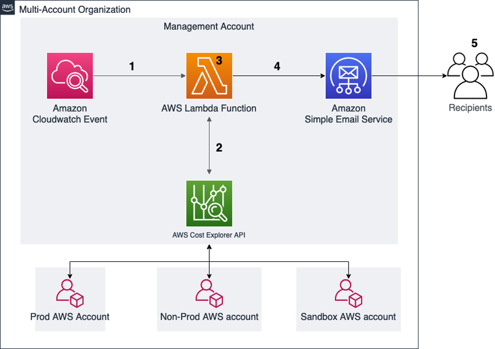
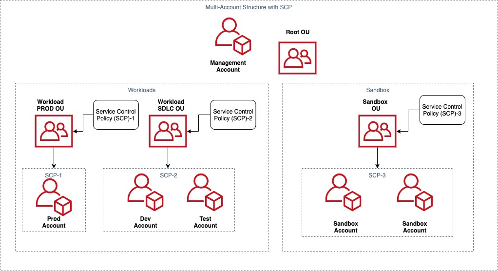
The following diagram illustrates how tagging works within SageMaker domains.

Before reviewing the implementation details, let’s explore several key SageMaker concepts: domain, project, project profile, and environment blueprint. For more information, refer to the SageMaker Unified Studio Administrator Guide.
- Domain – A domain is an organizing entity created by an administrator. Administrators assign users to domains to enable collaboration using similar tools, assets, and resources. A domain can represent a business organization or a business unit containing people who collaborate and share resources. After creating a domain, administrators share the URL with users to access the portal.
- Projects – Projects exist within each domain. A project provides a boundary where users can collaborate on a business use case. Users can create and share data, computing, and other resources within projects.
- Project profile – When you create a project, you must select a project profile. A project profile is a template that governs infrastructure for the project, simplifying project creation with preconfigured settings and resources ready for use.
- Environment blueprints – Environment blueprints are reusable templates for creating environments. They define settings for resource deployment and provide information for provisioning. Each blueprint uses an AWS CloudFormation template to create resources in a repeatable and scalable manner.
For effective cost tracking and allocation, make sure your SageMaker resources have proper tags. You can configure these as cost allocation tags to group and filter across AWS Billing and Cost Management tools (such as AWS Cost Explorer and AWS Data Exports).
As of this writing, SageMaker domains support tagging at the blueprint, domain, project, and environment level. When you create projects or add resources within an existing project, the following tags are automatically added to resources through CloudFormation resource tags, configured for each blueprint stack:
- AmazonDataZoneBlueprint – Type of blueprint corresponding to this blueprint’s CloudFormation template (for example, Tooling)
- AmazonDataZoneDomain – Amazon DataZone domain associated with this CloudFormation template
- AmazonDataZoneEnvironment – Amazon DataZone environment ID associated with this CloudFormation template
- AmazonDataZoneProject – Amazon DataZone project associated with this CloudFormation template
To track costs in SageMaker Unified Studio, you will perform the following steps:
- Create a SageMaker domain and project.
- Configure cost and billing settings by enabling cost allocation tags.
- (Optional) Generate costs for your project.
- Track costs using Cost Explorer and Data Exports.
Prerequisites
This post requires the following configurations in your AWS account:
- AWS IAM Identity Center enabled in your organization management account (preferred) or in the member account where you will use SageMaker Unified Studio. For instructions on enabling IAM Identity Center, refer to Enable IAM Identity Center.
- Cost Explorer enabled in your organization management account (preferred) or in the member account where you will use SageMaker Unified Studio. For configuration steps, refer to Enabling Cost Explorer.
Either legacy AWS Cost and Usage Reports (AWS CUR) with Amazon Athena integration or Data Exports configured and integrated with Athena for queries. For setup instructions, refer to creating Data Exports.
Create a SageMaker Unified Studio domain and project
Complete the following steps to set up your domain and project:
- Create a SageMaker Unified Studio domain using the Quick setup option (recommended for new users) or manual setup.
After domain creation, you will be redirected to the domain overview page.
- Choose Open Unified Studio.
- On the SageMaker Unified Studio console, choose Create project.
- For Project profile, choose SQL analytics, then choose Continue.

- Choose Continue to keep the default blueprint parameters.
- Review the configuration summary, then choose Create project.

After the project is created, you will be redirected to the project overview page. Record the project ID and domain ID.

Cost and billing configuration
As mentioned earlier, to track costs in SageMaker Unified Studio, you must configure cost allocation tags. Refer to Organizing and tracking costs using AWS cost allocation tags for more information about this feature.
Complete the following steps:
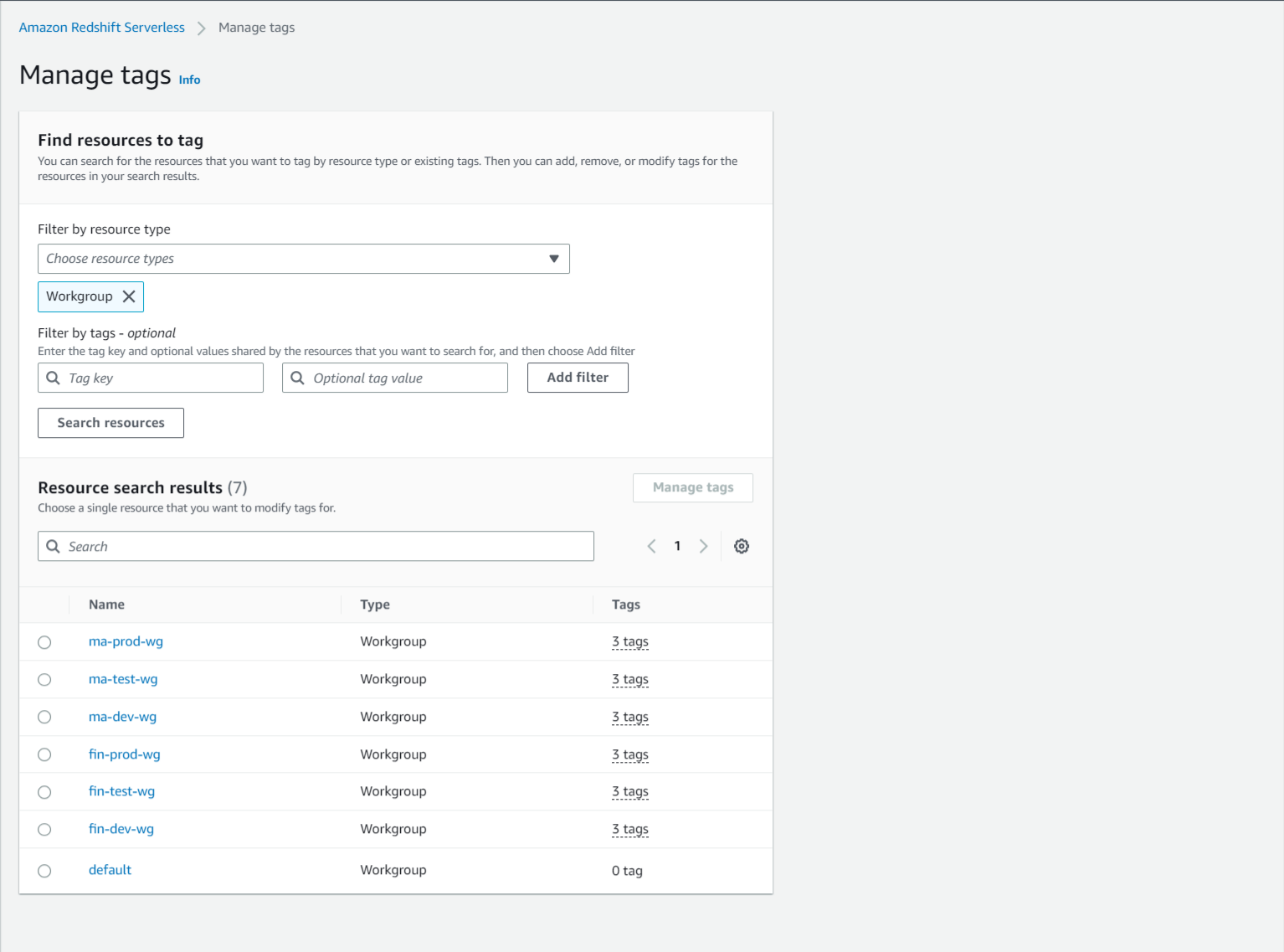
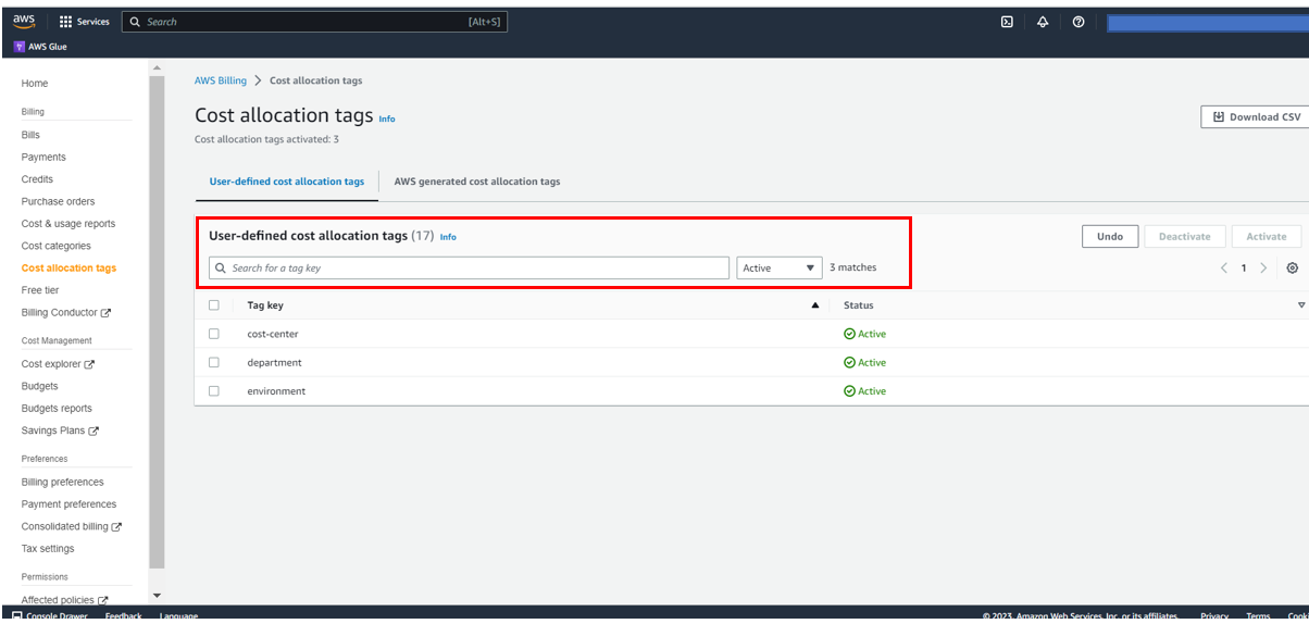
- On the AWS Billing and Cost Management console, under Cost organization in the navigation pane, choose Cost allocation tags.
- Select the following tags and choose Activate:
AmazonDataZoneDomainAmazonDataZoneProjectAmazonDataZoneEnvironmentAmazonDataZoneBlueprint
The AmazonDataZoneProject and AmazonDataZoneDomain tags correspond to the project and domain ID values you recorded earlier.

Cost allocation tags configuration doesn’t apply retroactively. If you want to monitor costs associated with these tags in the AWS Billing and Cost Management tools before the activation date, you must request a cost allocation tag backfill. The backfill operation can take several hours to complete.
Generate costs for the project
This section explains how to generate costs associated with the underlying data backend (Amazon Redshift in this case) to examine them using AWS billing tools. You can skip this section if you’re tracking costs on an active project.
To generate costs, we use the table structure used in the Redshift Immersion Labs. Refer to Create Tables for more details.
To run queries in SageMaker Unified Studio, follow these steps:
- In your project, choose New and then Query.

- Use the Amazon Redshift Serverless compute configured for the project to generate the costs:
- Choose the Redshift (Lakehouse) connection.
- Choose the
devdatabase. - Choose the
projectschema. - Choose Choose.

- Copy and execute the SQL statements provided in the following GitHub repo into the SageMaker Unified Studio query editor to create, load, and validate data on the tables.

After running these steps, you will have generated some Amazon Redshift costs that will be present for further analysis in AWS Billing and Cost Management tools. However, these tools (Cost Explorer and Data Exports) are refreshed least one time every 24 hours, so you might need to wait up to 24 hours before proceeding to the next section.
Tracking costs in AWS Billing and Cost Management tools
With the cost allocation tags enabled, you can use AWS Billing and Cost Management tools to analyze and track costs, including Cost Explorer and Data Exports. For more information about using these tools, refer to the AWS Billing and Cost Management User Guide.
Check costs in Cost Explorer
You can check your SageMaker Unified Studio costs using Cost Explorer. With this tool, you can view and analyze your costs and usage through an interface with pre-built filters and aggregation capabilities for various metrics. For more information, refer to the Analyzing your costs and usage with AWS Cost Explorer.
To access Cost Explorer, complete the following steps:
- On the AWS Management Console, choose your account name in the top right corner and choose Billing Dashboard, or search for “Cost Explorer” in the console search bar.
- On the Billing Dashboard, choose Cost Explorer in the navigation pane.
- For first-time users, choose Launch Cost Explorer to enable the service.
AWS can take up to 24 hours to prepare your cost data.
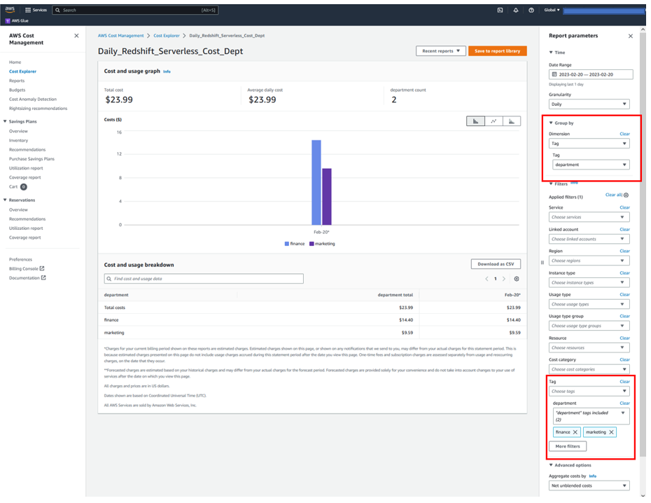
- To view overall costs per project, configure the following report parameters:
- For Date Range, enter your range.
- For Granularity, choose Monthly.
- For Dimension, choose Tag.
- For Tag, enter your tag (
AmazonDataZoneProject).

The following screenshot shows a sample report.

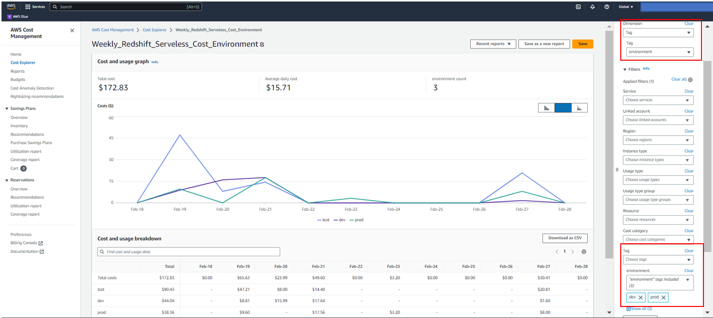
- To view different service costs for a specific project, update the following parameters:
- For Dimension, choose Service.

- For Tag¸ choose
AmazonDataZoneProjectand choose the value of the project you want to inspect (in this case,4z9d694nbsnyqx).
- For Dimension, choose Service.


The results should look similar to the following screenshot.

Check costs using Data Exports
With Data Exports, you can query your cost and usage in AWS with the maximum flexibility degree compared to other tools such as Cost Explorer. It provides a comprehensive set of measures and dimensions that you can include in the export to create a personalized report. This report is then delivered to Amazon Simple Storage Service (Amazon S3) so you can configure it with Athena, so it can be queried using SQL or business intelligence (BI) tools such as Amazon QuickSight.
This post assumes you have already configured a data export and you have it integrated with Athena (refer to Processing data exports for more information). For instructions on setting up CUR and Athena integration, refer to Creating reports.
Check costs by project
Use the following query to check costs by project:
Results will look similar to the following screenshot on the Athena console.

The preceding query shows your costs grouped by:
- Project (using tags)
- Service
- Product family, which corresponds to the subtype for a given product usage charge (for example, ML Instance for SageMaker, or Managed Storage for Amazon Redshift)
Check costs for individual projects
To check costs for a specific SageMaker Unified Studio project (for example, the sample project 4z9d694nbsnyqx created during this walkthrough), you can use the following query:
Monitor costs with Data Exports and QuickSight
If you enabled Athena to work with Data Exports, you can also configure QuickSight to query this data source. With QuickSight, you can create interactive dashboards to track SageMaker costs in SageMaker Unified Studio at scale.
Configure access and permissions
To create CUR dashboards in QuickSight, first complete the following steps:
- Subscribe to QuickSight and have an author user account. For instructions on subscribing to QuickSight, refer to Signing up for an Amazon QuickSight subscription.
- Enable access to Athena and your CUR S3 bucket in the Security & permissions section of the QuickSight administration console. You need QuickSight administrator permissions to access this console.

- If you’re using AWS Lake Formation, make sure your QuickSight user is authorized to query the CUR database and table. For more information about granting access in Lake Formation, refer to Granting permissions on Data Catalog resources.
Create a QuickSight dataset
The next step is to create a dataset in QuickSight using a SQL query. For instructions on creating a dataset with SQL, refer to Using SQL to customize data. Use the following SQL expression:

The preceding query includes only cost and usage data that’s tagged with either user_amazon_data_zone_environment or user_amazon_data_zone_project to focus on SageMaker associated costs. To include other AWS costs, you must modify these filters.
Create QuickSight dashboards
Using the authoring capabilities of QuickSight, you can create interactive dashboards where business stakeholders can explore and track costs associated with SageMaker Unified Studio projects. You can use these dashboards to review relevant cost metrics at a glance that are derived from the Data Exports dimensions and metrics included in your dataset, as shown in the following screenshot. For more information about adding visuals to analyses, refer to Adding visuals to Amazon QuickSight analyses.

The preceding example shows a dashboard built using QuickSight connected to a Data Exports dataset. The dashboard contains the following visuals:
- KPI visual showing the current monthly costs for SageMaker Unified Studio along with the month over month (MoM) variation and history
- Autonarrative visual analyzing SageMaker Unified Studio costs (highest) by month
- Vertical stacked bar chart showing SageMaker Unified Studio costs by month (grouped by project)
- Donut chart showing SageMaker Unified Studio cost by service
- Heat map visual correlating costs by project ID and service
Using this approach (QuickSight and Data Exports), you can create highly customizable dashboards to explore and monitor your SageMaker Unified Studio costs. Furthermore, you can create automated reports using the QuickSight reporting feature to send these by email to the relevant stakeholders.
Clean up
Delete the resources you created as part of this post when you’re done with them to avoid monthly charges. This includes SageMaker resources, created Data Export reports and the QuickSight subscription (in case it was created to visualize costs).
- Delete SageMaker resources
- Log in to the SageMaker domain using an admin role.
- Delete the project you created.
- Delete the SageMaker domain.
- Delete Data Exports reports
- On the AWS Billing console, in the navigation pane, choose Cost & Usage Reports.
- Select the report you want to delete.
- Choose Delete.
- Confirm the deletion by choosing Delete report.
For more information about managing Data Exports, refer to Deleting exports.
- Unsubscribe from QuickSight
- On the QuickSight console, choose your profile name in the top right corner.
- Choose Manage QuickSight.
- Choose Account settings.
- At the bottom of the page, choose Delete your QuickSight account.
- Review the information about data deletion.
- Enter
deleteto confirm. - Choose Delete.
IMPORTANT NOTE: Before unsubscribing, make sure you backed up any dashboards or analyses you want to keep. After deletion, you can’t recover your QuickSight assets. For more information about managing your QuickSight subscription, refer to Deleting your Amazon QuickSight subscription and closing the account.
Conclusion
Managing costs on a unified platform like SageMaker can seem challenging because it aggregates many tools and services with different cost models. In this post, we showed how to use AWS Billing and Cost Management tools to aggregate and categorize costs across the various services used within SageMaker. With this approach, you can monitor and track respective service costs, either in aggregate or focusing on a particular project.
Start taking control of your analytics and ML costs today. With AWS Billing and Cost Management tools with SageMaker, you can:
- Track and monitor your service costs
- Break down expenses by project or service
- Implement efficient back charging mechanisms to the different business units or organizations using SageMaker within your organization
For further reading, refer to Analyzing your costs and usage with AWS Cost Explorer and Processing Data Exports (using Athena).
About the authors
 Enrique Salgado Hernández is a Senior Specialist Solutions Architect at AWS with more than 10 years of experience working in the cloud. He specializes in designing and implementing large-scale analytics architectures across various industry sectors. He is passionate about working with customers to solve their problems by supporting them during their cloud journey.
 Angel Conde Manjon is a Senior EMEA Data & AI PSA, based in Madrid. He previously worked on research related to data analytics and AI in diverse European research projects. In his current role, Angel helps partners develop businesses centered on data and AI.


 Nikhil Agarwal is a Sr. Technical Manager with Amazon Web Services. He is passionate about helping customers achieve operational excellence in their cloud journey and actively working on technical solutions. He is an artificial intelligence (AI/ML) and analytics enthusiastic, he deep dives into customer’s ML and OpenSearch service specific use cases. Outside of work, he enjoys traveling with family and exploring different gadgets.
 Rick Balwani is an Enterprise Support Manager responsible for leading a team of Technical Account Mangers (TAMs) supporting AWS independent software vendor (ISV) customers. He works to ensure customers are successful on AWS and can build cutting-edge solutions. Rick has a background in DevOps and system engineering.
 Ashwin Barve is a Sr. Technical Manager with Amazon Web Services. In his role, Ashwin leverages his experience to help customers align their workloads with AWS best practices and optimize resources for maximum cost savings. Ashwin is dedicated to assisting customers through every phase of their cloud adoption, from accelerating migrations to modernizing workloads.
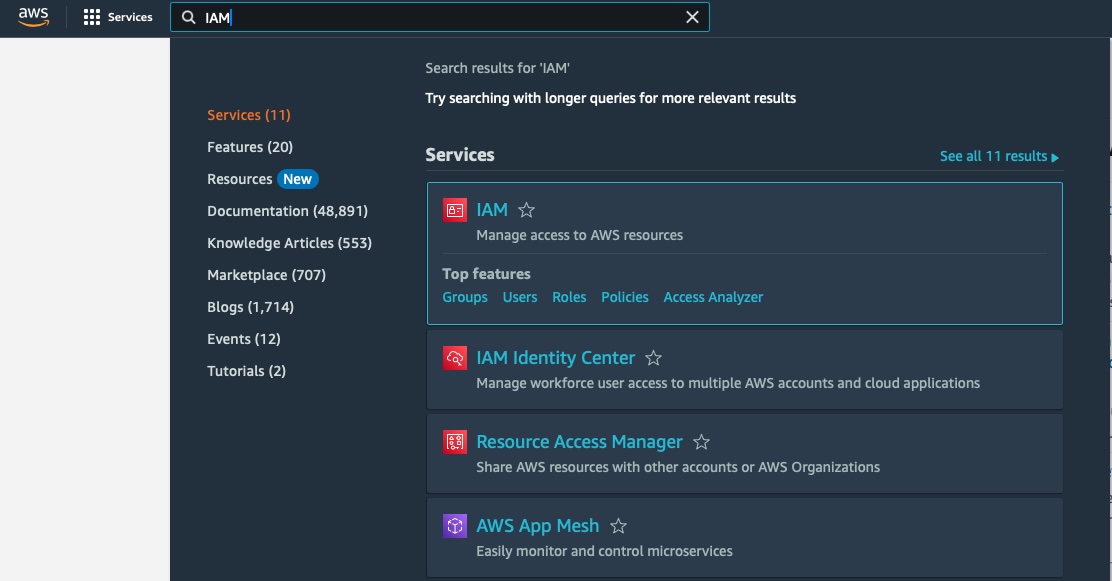


 Noritaka Sekiyama is a Principal Big Data Architect on the AWS Glue team. He is responsible for building software artifacts to help customers. In his spare time, he enjoys cycling with his new road bike.


 Sandeep Bajwa is a Sr. Analytics Specialist based out of Northern Virginia, specialized in the design and implementation of analytics and data lake solutions.