Post Syndicated from Ramkumar Nottath original https://aws.amazon.com/blogs/big-data/extract-prepare-and-analyze-salesforce-com-data-using-amazon-appflow-aws-glue-databrew-and-amazon-athena/
As organizations embark on their data modernization journey, big data analytics and machine learning (ML) use cases are becoming even more integral parts of business. The ease for data preparation and seamless integration with third-party data sources is of paramount importance in order to gain insights quickly and make critical business decisions faster.
AWS Glue DataBrew is a visual data preparation tool that cleans and normalizes data without writing code. This reduces the time it takes to prepare data for analytics and ML by up to 80% compared to traditional approaches to data preparation.
Software as a service (SaaS) applications play a pivotal role in organizations’ analytics pipelines. This data is essential to include when performing analytics to get insights to make better business decisions. Amazon AppFlow is a fully managed integration service that helps you transfer SaaS data to your data lake securely.
Recently, DataBrew announced native console integration with Amazon AppFlow to connect to data from applications like Salesforce, Zendesk, Slack, ServiceNow, and other SaaS applications, and AWS services like Amazon Simple Storage Service (Amazon S3) and Amazon Redshift. With native integration with Amazon AppFlow, DataBrew is addressing both the challenges with data preparation and seamless integration with SaaS applications.
Salesforce is a popular and widely used customer relationship management (CRM) platform. It lets you store and manage prospect and customer information—like contact info, accounts, leads, and sales opportunities—in one central location. You can derive a lot of useful information by combining the prospect information stored in Salesforce with other structured and unstructured data in your data lake.
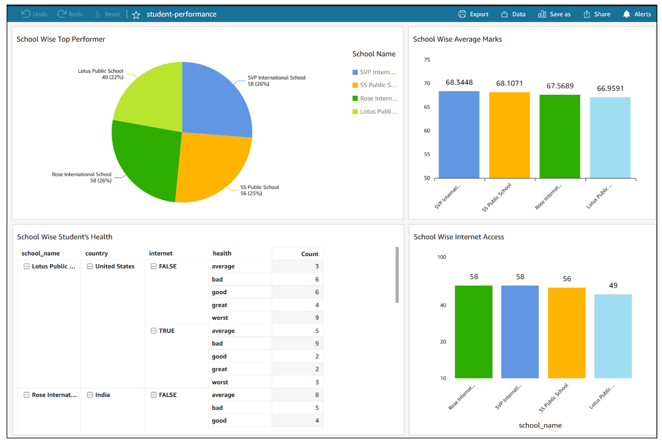
In this post, we walk you through how to extract data from Salesforce.com using the native integration that DataBrew has with Amazon AppFlow, prepare the data for your analytical use cases using DataBrew, store it in Amazon S3, and query it with Amazon Athena.
Architecture overview
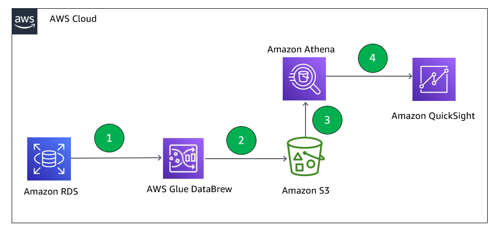
The following diagram represents the flow described in this post. With the visual point-and-click interface in Amazon AppFlow, you create a new flow with Salesforce as source. You can either use an existing connection to Salesforce or create a new one. In DataBrew, while creating a dataset, you can choose the Amazon AppFlow flow as one of the sources to import the data for data preparation. After you perform the data preparation steps on sample data, you can save the steps as a recipe and automate the flow by creating a DataBrew job by selecting the dataset for the source and the newly created recipe for transformation. The transformed data is published to an S3 bucket. You can use an AWS Glue crawler to catalog that data and use Athena to query the data.

The workflow includes the following steps:
- Create an S3 bucket for the raw and transformed data.
- Create a connection to Salesforce.
- Create a flow to extract the data from Salesforce.com.
- Create a dataset and project.
- Prepare the data and create a recipe.
- Create a job to pull the data from the Amazon AppFlow flow, run the transformations, and load the data in Amazon S3.
- Create a crawler to catalog the data.
- Analyze data using Athena.
Prerequisites
To implement this solution, you need the following prerequisites:
- An AWS account
- AWS Identity and Access Management (IAM) role permissions to access Amazon S3, Amazon AppFlow, DataBrew, and Athena
- A Salesforce.com account
Now that we have discussed the architecture of our solution, we present the step-by-step instructions.
Create an S3 bucket
To create an S3 bucket, complete the following steps:
- On the Amazon S3 console, choose Create bucket.
- Enter a name for your bucket; for example,
databrew-appflow-data-prep-<your name>. - Choose Create bucket.
Create a connection to Salesforce
If you already have a Salesforce connection created in Amazon AppFlow, you can skip this step. To create a new connection, complete the following steps:
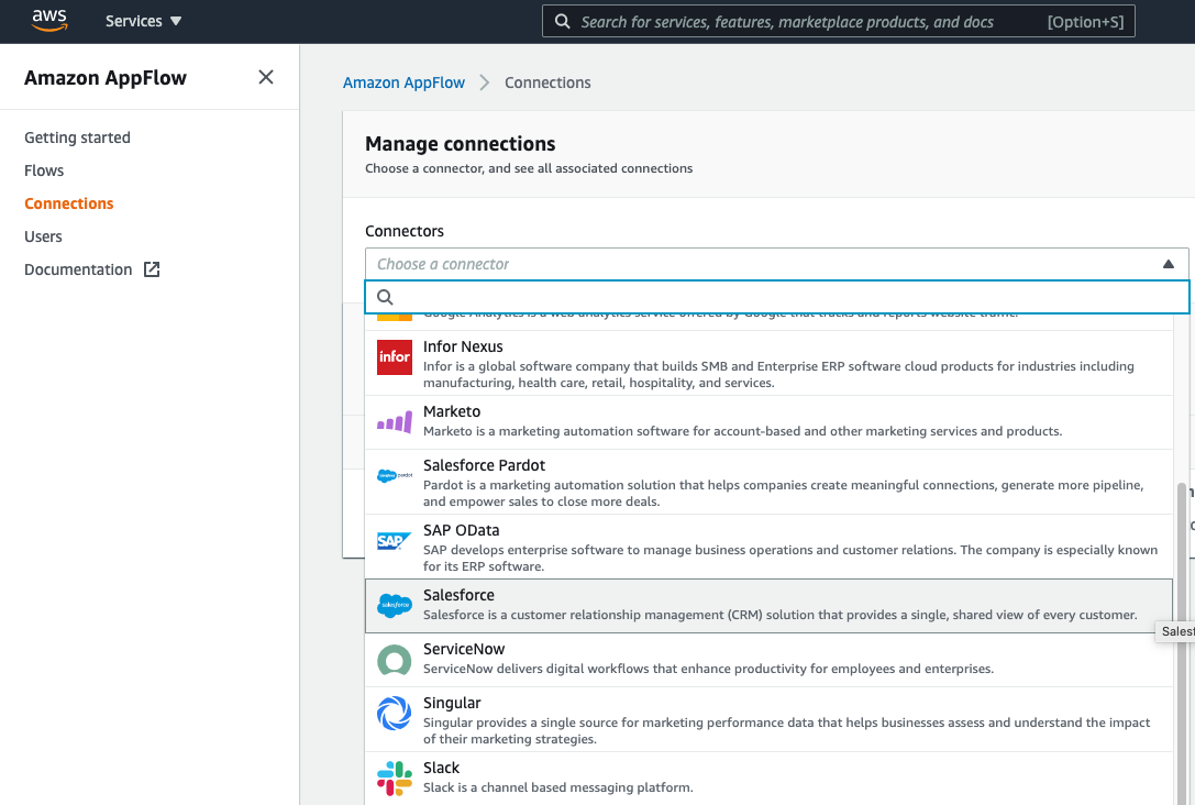
- On the Amazon AppFlow console, choose Connections in the navigation pane.

- From the list of connectors, choose Salesforce.

- Choose Create connection.
- For Connection name, enter a name (for example,
sfdc-appflow). - Choose Continue.
- You’re redirected to a sign-in screen where you can log in to your Salesforce account. If you don’t have a Salesforce account, you can sign up for a developer account.

- Choose Allow to allow Amazon AppFlow to access your Salesforce account.


You can now see the new connection that was created.
Create a flow in Amazon AppFlow to extract data from Salesforce.com
To create a flow in Amazon AppFlow, complete the following steps:
- On the Amazon AppFlow console, choose Flows in the navigation pane.
- Choose Create flow.
- On the Specify flow details page, enter a name for the flow (for example,
salesforce-data). - Optionally, provide a description for the flow and tags.
- Choose Next.
- On the Configure flow page, for Source name¸ choose Salesforce.
- Choose the connection we created in the previous step.
- For Choose Salesforce object, choose the object you want to work with (for this post, we choose Opportunity).

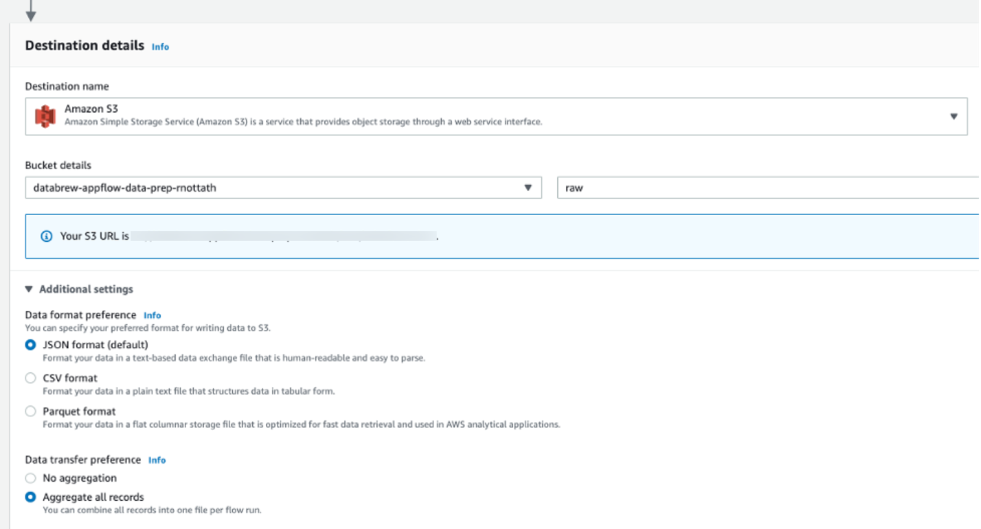
- For Destination name, choose Amazon S3.
- For Bucket details, choose the bucket you created earlier.
- Optionally, provide a prefix (folder) where you want the data to land within the bucket.
- Under Additional settings, for Data transfer preference, select Aggregate all records.

- For Choose how to trigger the flow¸ select Run on demand.

- Choose Next.
- On the Source to destination field mapping page, for Source field name, select the fields you want to work with and choose Map fields directly.


Alternatively, you can choose Map all fields directly to map all the fields from the object.

- On the Add filters page, add any filters for the data you’re pulling.
- On the Review and create page, review all the details and choose Create flow.
- After the flow is created, choose Run flow to run the flow and verify whether the flow ran successfully.
Create a dataset and project in DataBrew
To create a dataset and DataBrew project, complete the following steps:
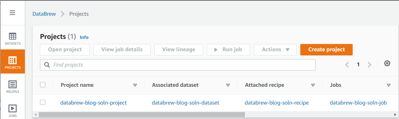
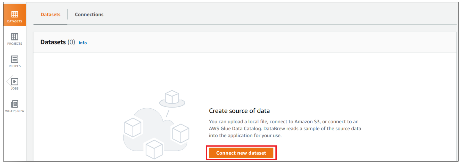
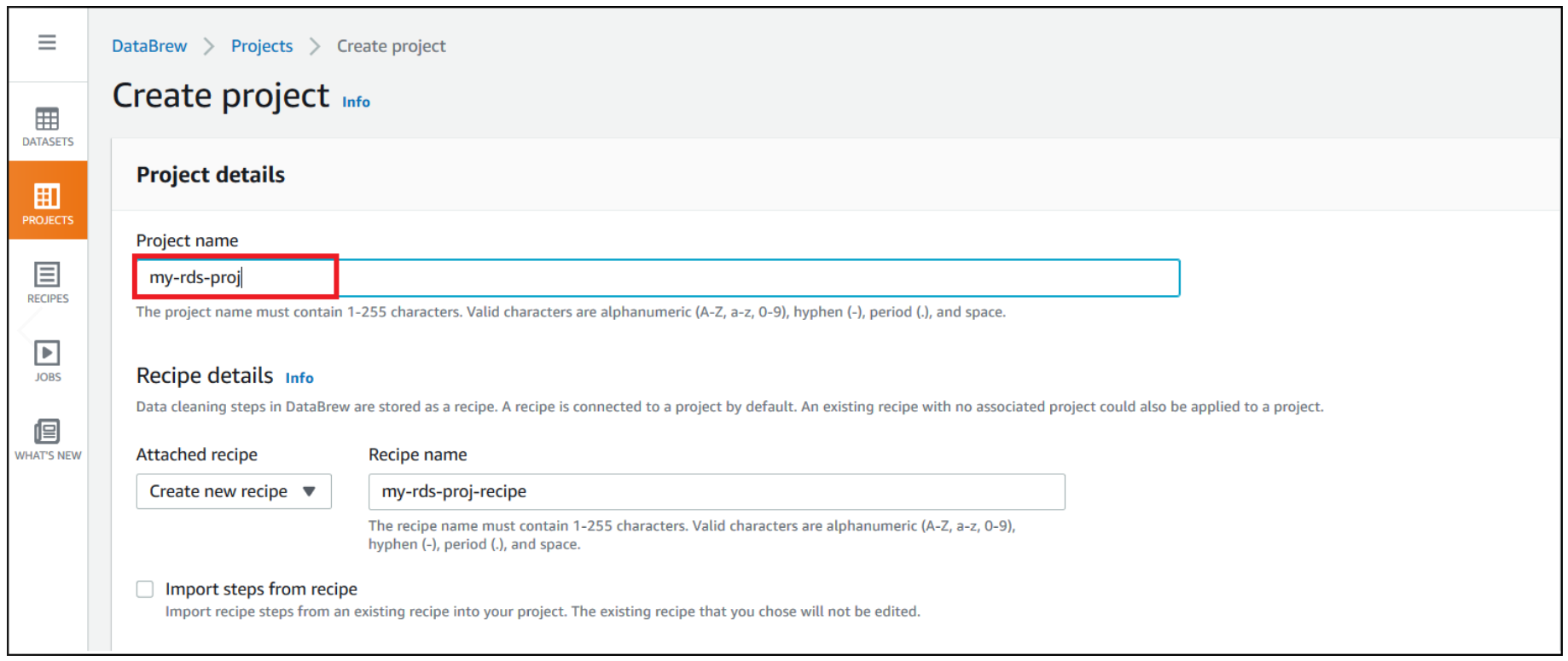
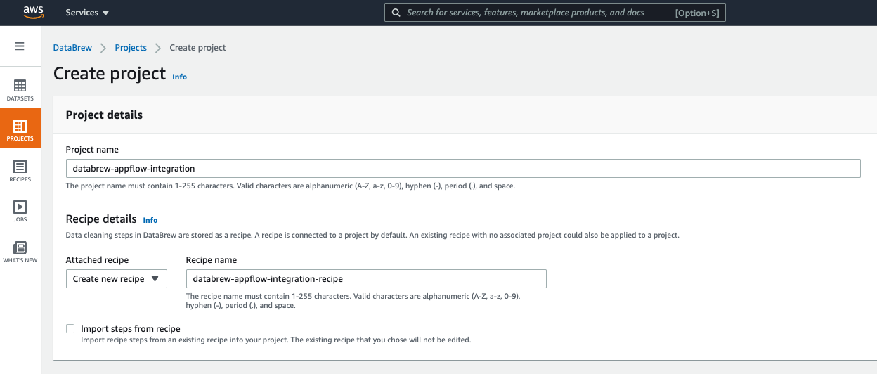
- On the DataBrew console, choose Projects in the navigation pane.
- Choose Create project.
- For Project name, enter a name (for example,
databrew-appflow-integration).

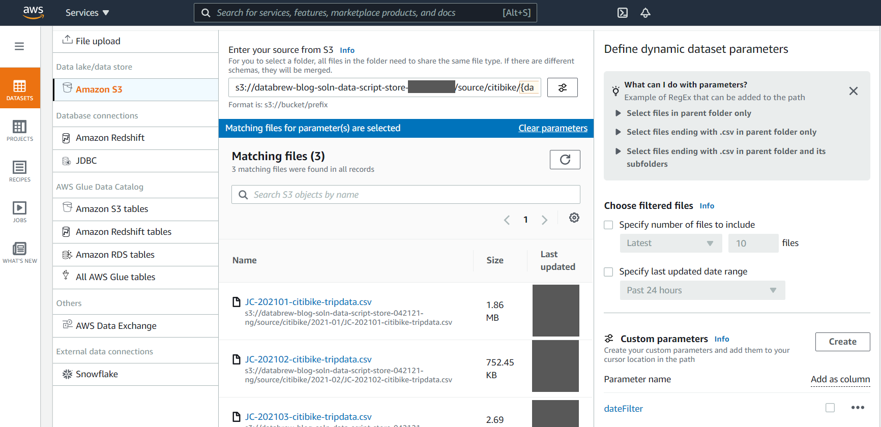
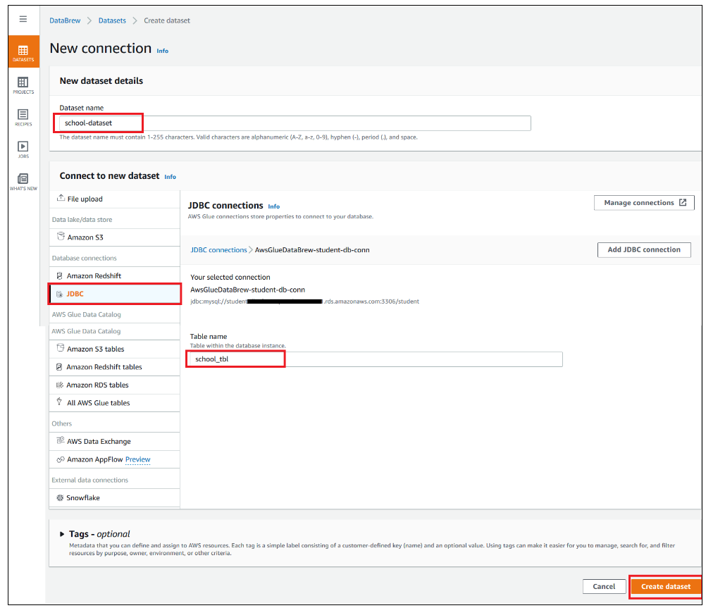
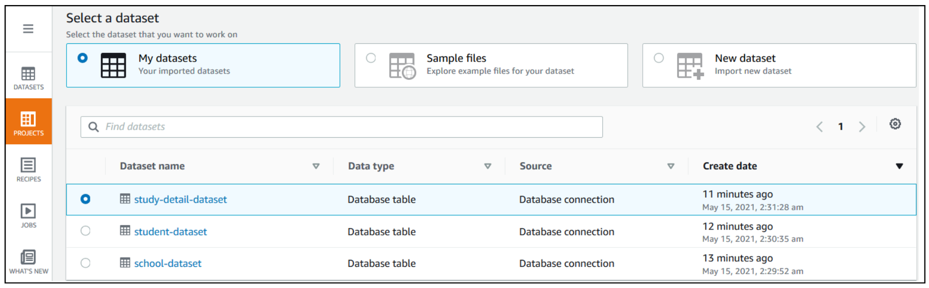
- For Select a dataset, select New dataset.
- For Dataset name, enter a name (for example,
databrew-sfdc). - From the list of sources, choose Amazon AppFlow.
- Select the flow you created.

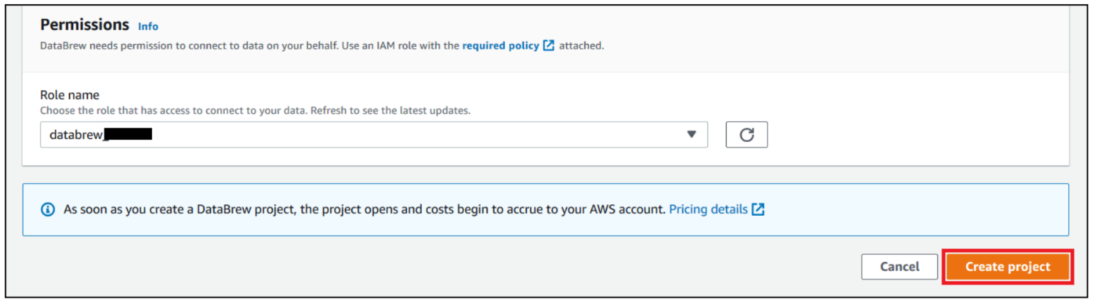
- Under Permissions, for Role name, choose Create new IAM role.
- For New IAM role suffix, enter a suffix (for example,
appflow-databrew). - Choose Create project.


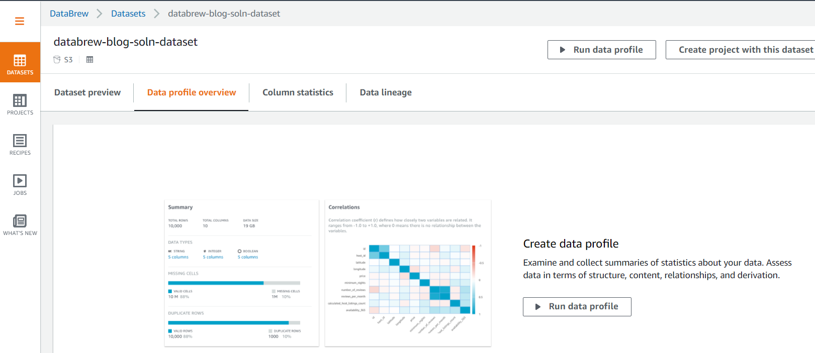
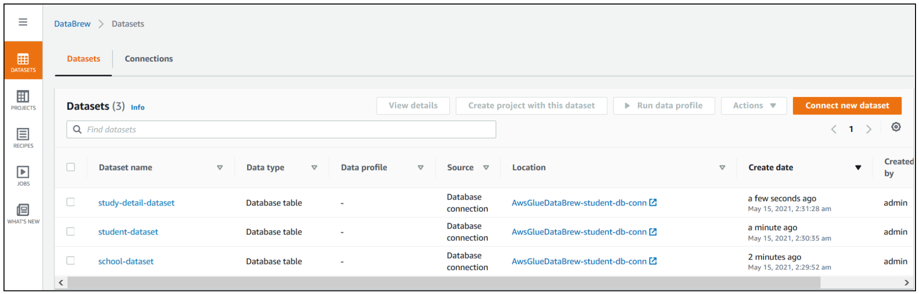
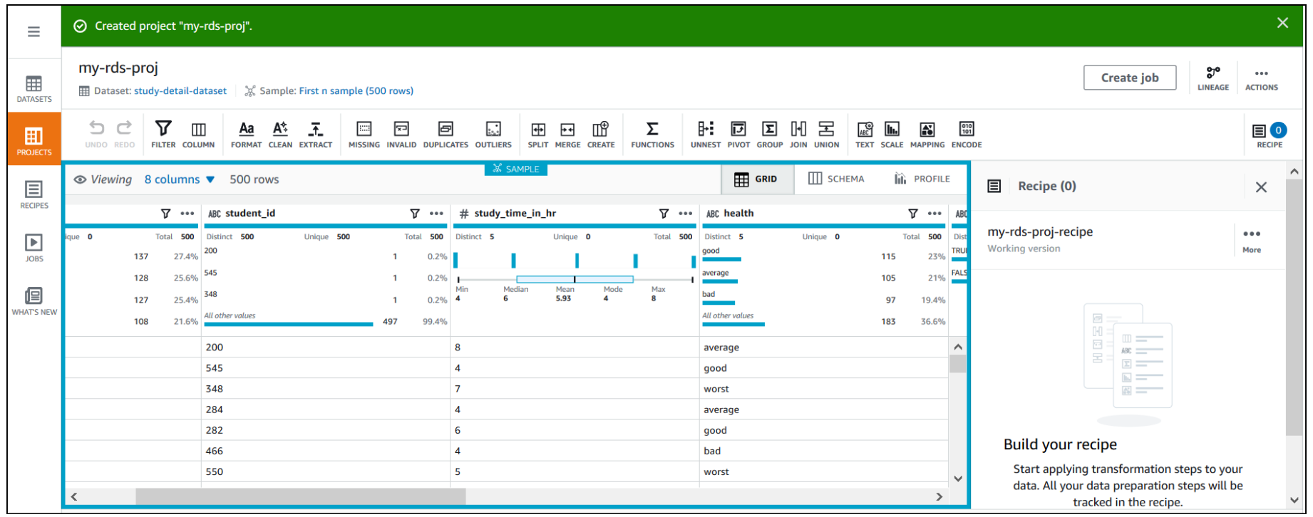
After you create the project, data is loaded to DataBrew so that you can perform data preparation activities.
Prepare data and create a recipe
With DataBrew, you can choose from over 250 pre-built transformations to automate data preparation tasks, all without the need to write any code. In this post, we only discuss a few of them. For the full list of transformations, see Recipe step and function reference.
In this step, we split the CloseDate column to CloseYear, CloseMonth, and CloseDay. Then we flag the outliers in the Amount column.
- Duplicate the column
CloseDateby choosing the column and choosing Duplicate.

- For Duplicate column name, enter a name.
- Choose Apply.
- Select the column you created and on the Clean menu, choose Replace value or pattern.

- For Value to be replaced, select Enter custom value and enter -.
- Choose Apply.

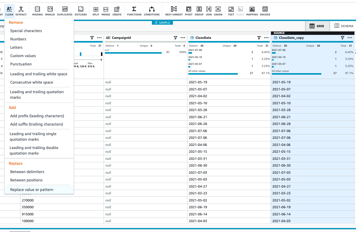
This replaces – with empty values.

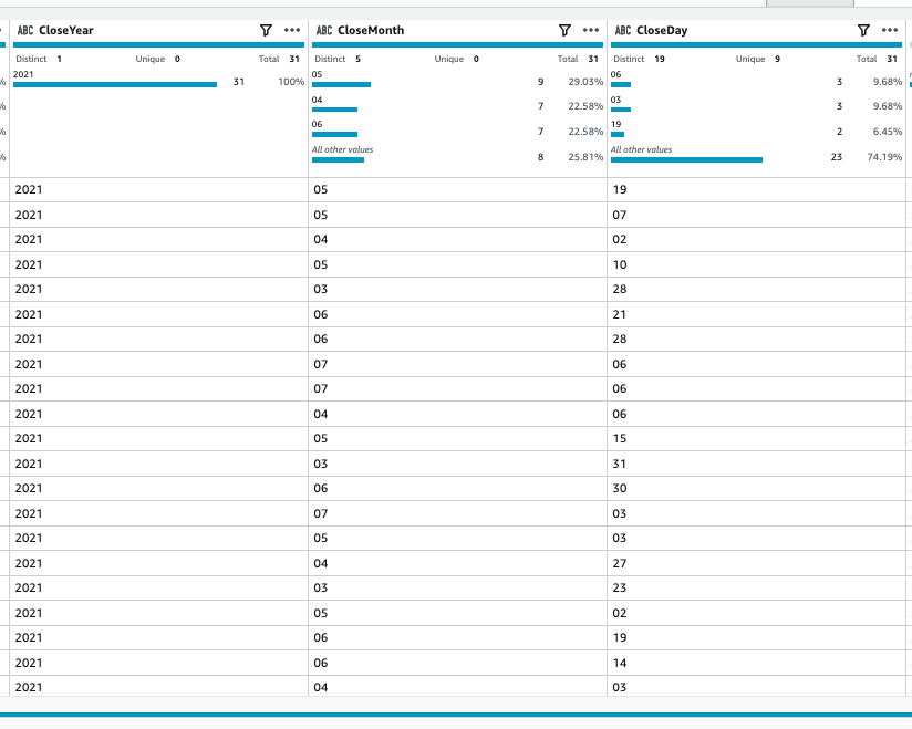
- Select the modified column and on the options menu, choose Split menu and At positions from beginning.

- For Position from the beginning¸ enter
4. - Choose Apply.

This creates a new column with the year value.

Next, we split the column at position 2 from the beginning in CloseDate_copy_2 to extract month and day.
- On the options menu, choose Split column.

- Rename the
CloseDate_copy_1column toCloseYearand choose Apply.

- Repeat the steps to rename the other two newly created columns to
CloseMonthandCloseDay.

- Select the Amount column and on the Outliers menu, choose Flag outliers.
- For Standard deviation threshold, enter
3.

- Under Outlier actions, select Flag outliers.
- Choose Apply.


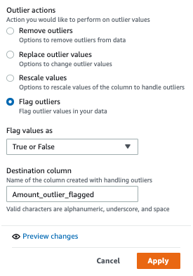
You can see that an additional column got added and the outliers are flagged.

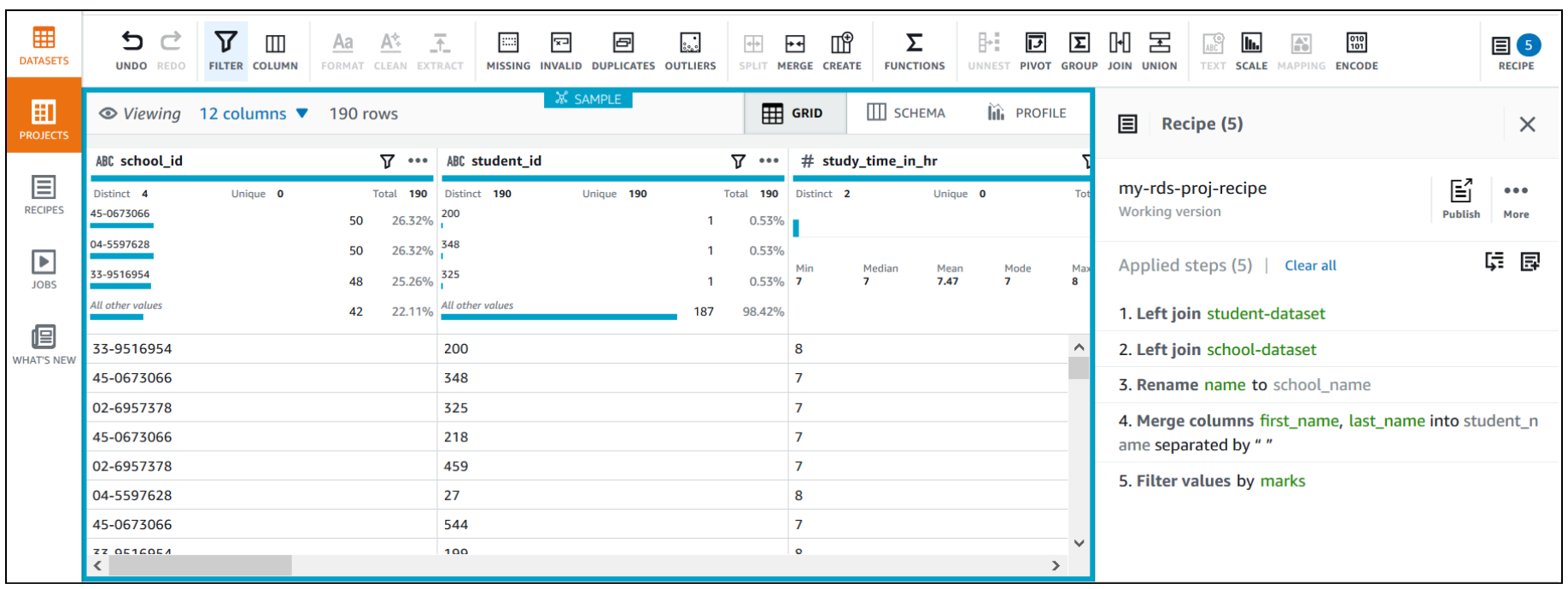
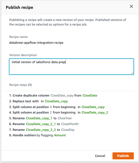
All the steps that we performed so far are recorded under Recipe.
- Under Recipe, choose Publish.

- For Version description, enter a description.
- Choose Publish.

This saves the recipe for future use.
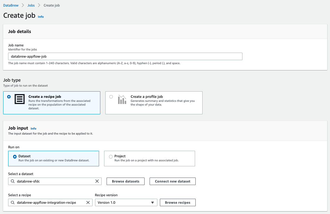
Create a DataBrew job
To create a DataBrew job, complete the following steps:
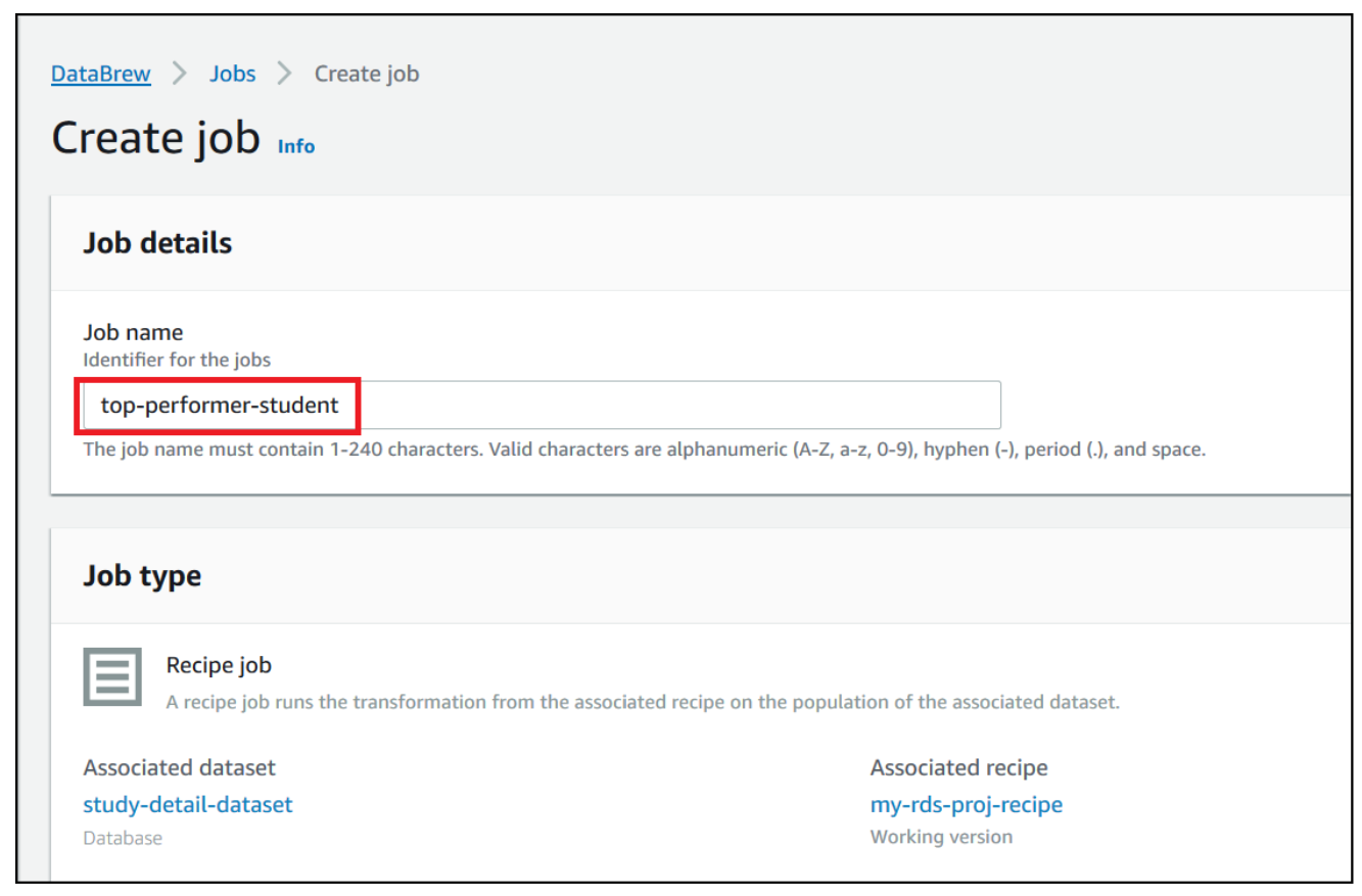
- On the DataBrew console, choose Jobs in the navigation pane.
- Choose Create job.
- For Job name, enter a name (for example,
databrew-appflow-job). - For Select a dataset, choose the dataset we created (
databrew-sfdc). - For Select a recipe, choose the recipe we created (
databrew-appflow-integration-recipe).

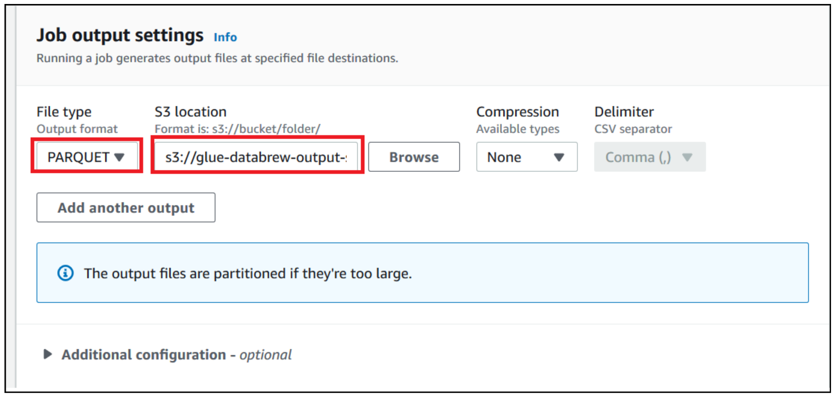
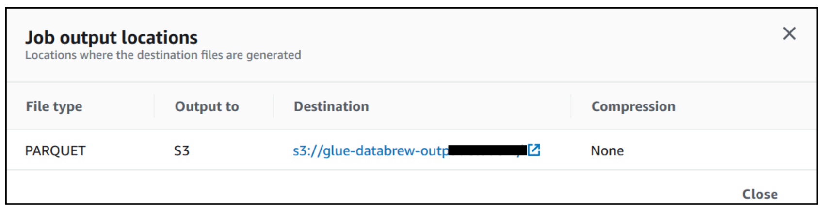
- In the Job output settings section, for Output to, choose Amazon S3.
- For S3 location, enter the S3 path for the data (for example,
s3://databrew-appflow-data-prep-<your name>/processed/).

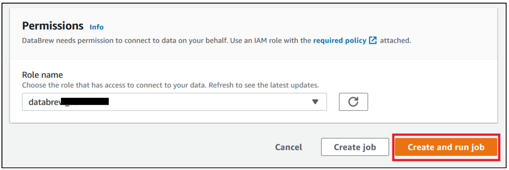
- For Role name, choose the role with suffix
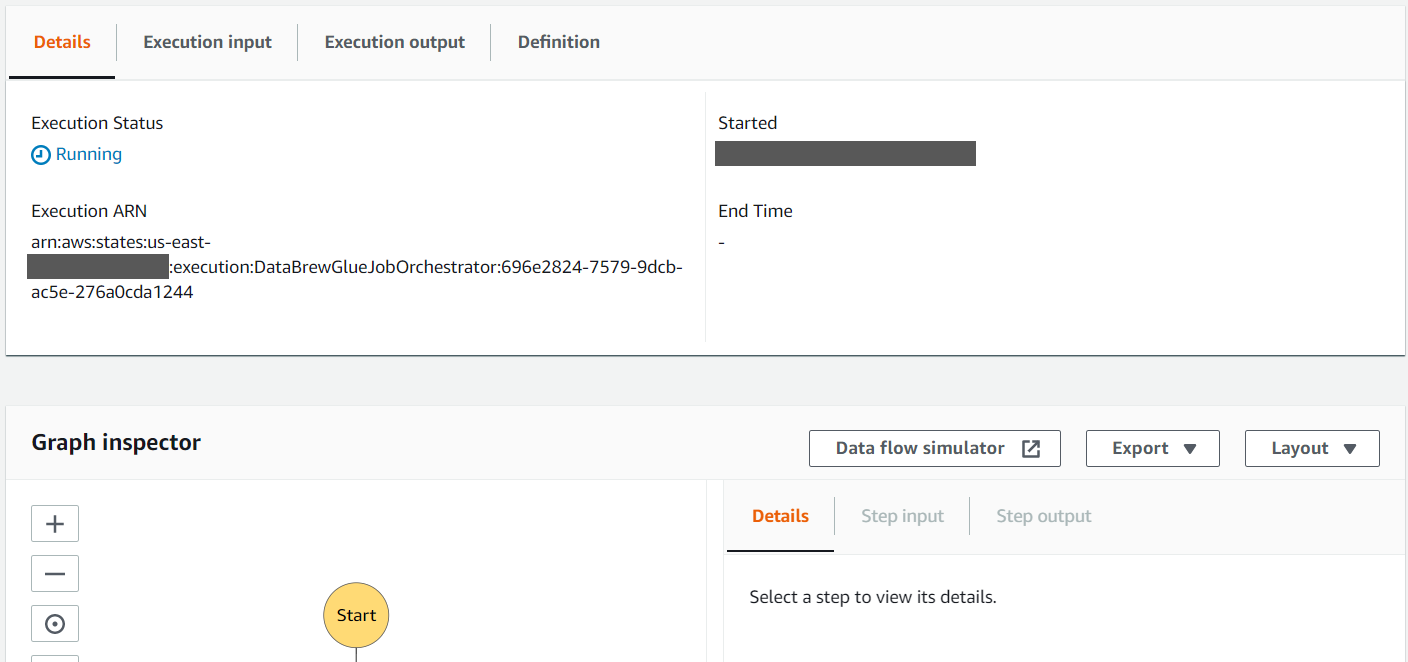
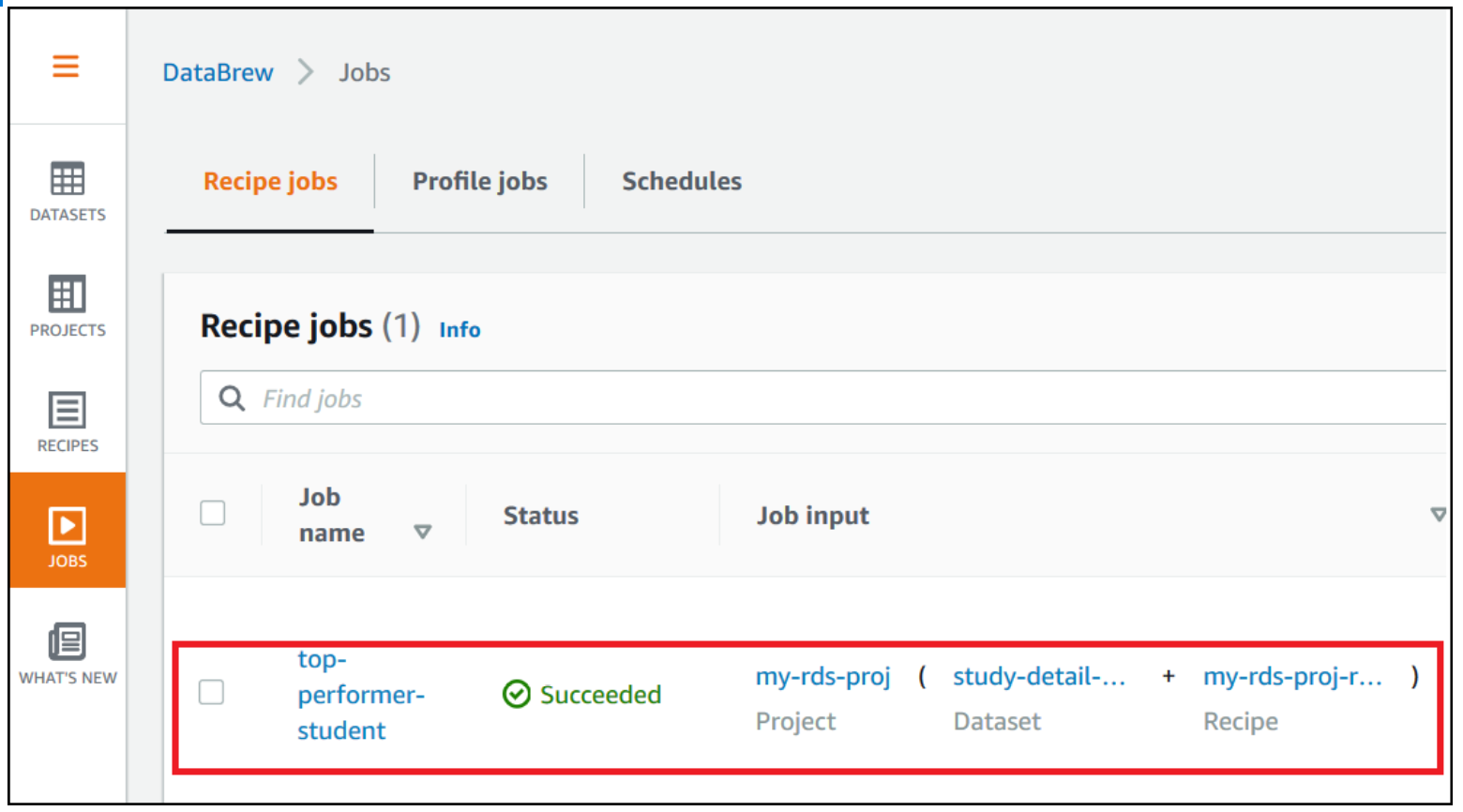
databrew-appflow-role. - Choose Create and run job.


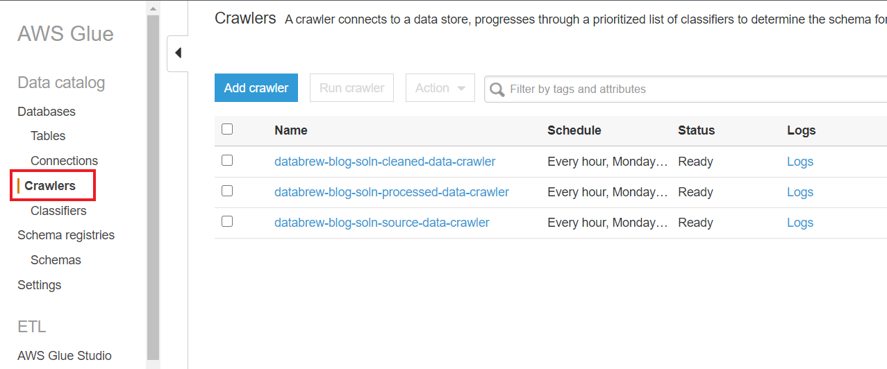
Create a crawler to catalog the data
To create your AWS Glue crawler, complete the following steps:
- On the AWS Glue console, choose Crawlers.
- Choose Add crawler.
- For Crawler name¸ enter a name (for example,
databrew-opportunity-data). - Choose Next.
- Under Specify crawler source type, keep the default options and choose Next.
- Under Add a data store, for Include path, choose the S3 bucket that we used for the processed data (for example,
s3://databrew-appflow-data-prep-<your name>/processed). - Choose Next.
- For Add another data, select No.
- Choose Next.
- Select Create an IAM role and provide a suffix for the role (for example,
databrew). - For Frequency, choose Run on demand.
- On the next page, choose Add database.
- Enter a database name (for example,
databrew-appflow). - Choose Create.
- For Prefix, enter
opportunity_. - Choose Next.
- Review the details and choose Finish.
- After the crawler is created, select it and choose Run crawler.
The crawler catalogs the data that we uploaded to Amazon S3 after processing using DataBrew.
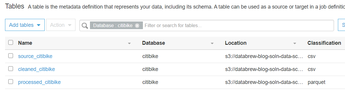
Analyze data using Athena
When the crawler is complete, we can analyze the data with Athena.
- On the AWS Glue console, choose the database we created.
- Under Data catalog, choose Tables in databrew-appflow.
You can see a table named opportunity_processed, which points to the Amazon S3 location where the processed data was landed.
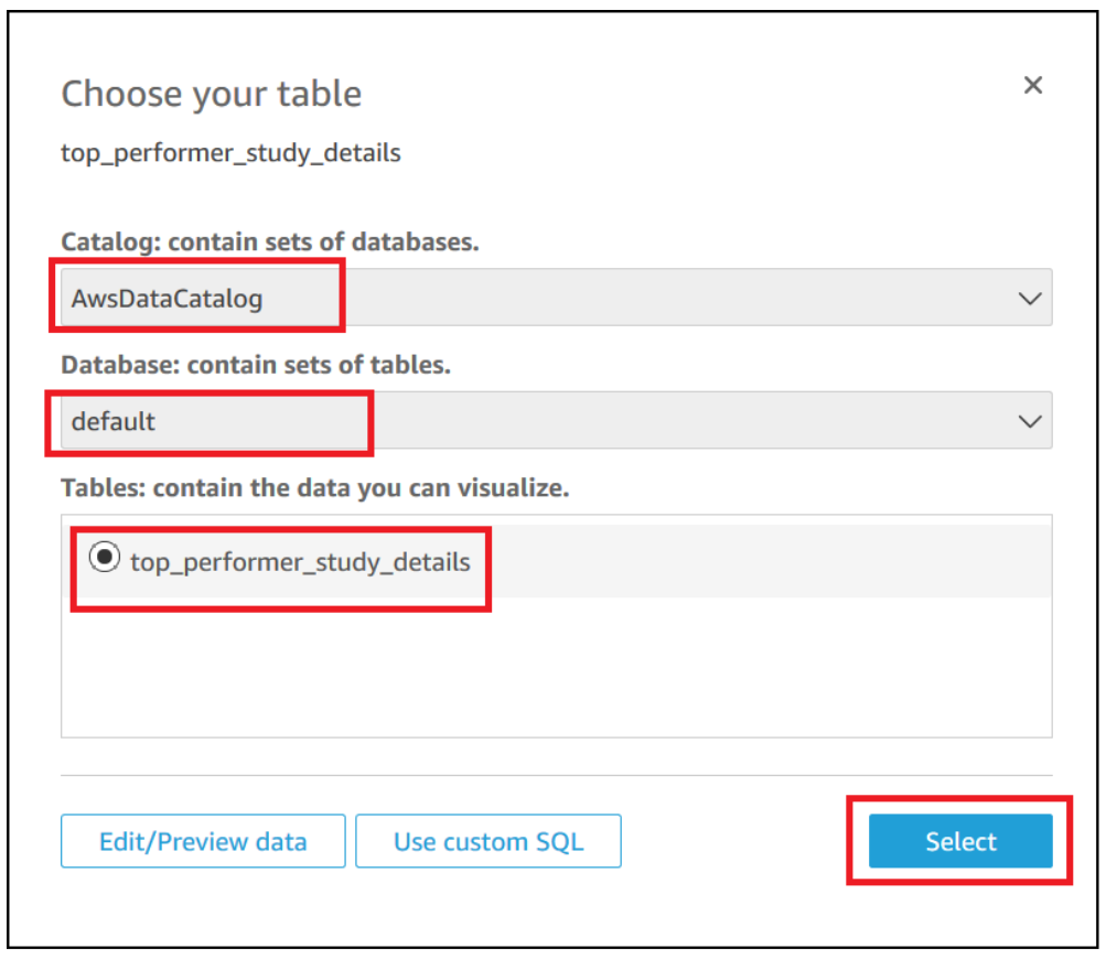
- Select the table name.
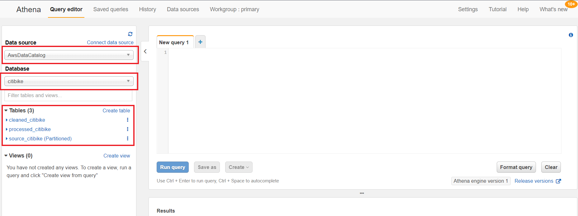
- On the Action menu, choose View data.
A pop-up may appear to let you know that you’re going to the Athena console.
- Choose Preview data.
If this is the first time using Athena in this account, you have to set the query result location.
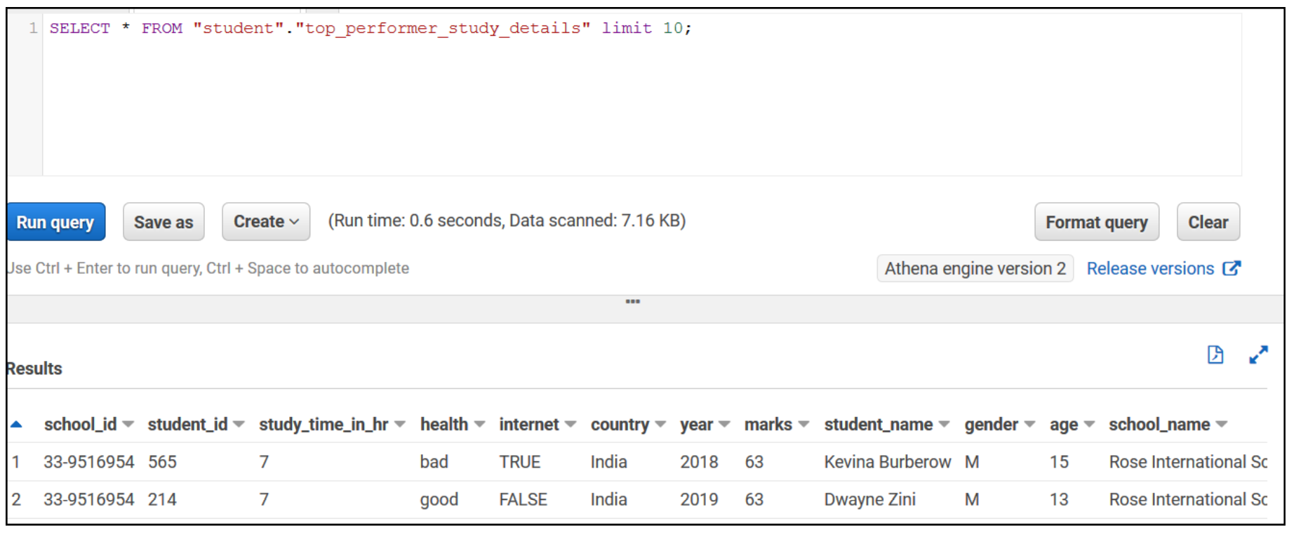
- Run a query in Athena.
You should be able to see the data in Amazon S3.

You can perform further analysis by running more queries on the data. The following query returns the expected revenue for based on various closeyear and closemonth combinations of opportunities:

Clean up
You may want to clean up the demo environment when you are done. To do so, delete the following resources that were created as part of this post:
- S3 bucket (
databrew-appflow-data-prep-<your name>) - Connection to Salesforce in Amazon AppFlow (
sfdc-appflow) - Flow in Amazon AppFlow (
salesforce-data) - Dataset (
databrew-sfdc), project (databrew-appflow-integration), and job (databrew-appflow-job) in DataBrew - AWS Glue Data Catalog database (
databrew-appflow) - IAM role (
AWSGlueDataBrewServiceRole-appflow-databrew)
Conclusion
In this post, we walked you through how to extract data from Salesforce.com using the native integration that DataBrew has with Amazon AppFlow. We also demonstrated how to prepare the data for analytical use cases using DataBrew, operationalize the data preparation steps by creating a recipe and use that in a DataBrew job, store the job result in Amazon S3, and query it with Athena.
If you have any questions or suggestions, please leave a comment.
About the Authors
 Ramkumar Nottath is a Sr. Solutions Architect at AWS focusing on Analytics services. He enjoys working with various customers to help them build scalable, reliable big data and analytics solutions. His interests extend to various technologies such as analytics, data warehousing, streaming, and machine learning. He loves spending time with his family and friends.
 Srikanth Sopirala is a Principal Analytics Specialist Solutions Architect at AWS. He is a seasoned leader with over 20 years of experience, who is passionate about helping customers build scalable data and analytics solutions to gain timely insights and make critical business decisions. In his spare time, he enjoys reading, spending time with his family, and road cycling.