At Grab, our journey towards a more robust and scalable data ecosystem has been a continuous evolution.
Considering the size of our data lake and complexity of our ecosystem, with businesses spanning across ride hailing, food delivery, and financial services, we have been long past the point where a single centrally managed data warehouse could serve all these data needs. Over its first decade, Grab experienced dramatic growth. Like most growing businesses, teams in Grab prioritised delivering new features to meet the demands of their users. This meant that the task of data maintenance had to take a back seat so that development and stabilisation works can be focused to keep up with the growth. However, to prepare Grab for the next 10 years, especially for a future where AI is likely to play an important role, our leadership understood the need for high quality data foundation and gave a mandate to our data teams to uplevel our entire enterprise data ecosystem.
Acknowledging the rising need for data-driven insights and the continuous expansion of our data repository, we initiated our data mesh journey, named the Signals Marketplace, in 2024.
However, this journey was far from simple. We encountered several critical challenges that required a significant transformation in our approach to data management. Some of the challenges encountered include:
High volume and variety of data being generated: Grab’s diverse operations created both opportunities and complexities. Effectively harnessing this wealth of information required a scalable, streamlined and accessible approach.
Gaps in data ownership: As our data landscape expanded, maintaining data quality and reliability became increasingly difficult without clear lines of ownership and accountability. This often led to ad-hoc discussions and delays in resolving data related issues. Since it was difficult to trust the reliability of an existing pipeline, teams were likely to create duplicate pipelines just so they have something they can control.
Unscalable reliance on central Data Engineering (DE) team: Our traditional reliance on a central DE team to curate and serve all data needs was becoming a bottleneck. This centralised model struggled to keep pace with the distributed nature of data creation and consumption across various product and engineering teams.
Lack of communication between data consumers and producers: Data producers are unaware of downstream dependencies of their data which led to several instances of critical pipelines breaking because of upstream changes.
No single source of truth: While we did have a central data warehouse, it still left a lot of data gaps across Grab’s many business lines. Teams would struggle to identify the correct data definitions and reliable sources of truth.
Varied sophistication of data practitioners: Different teams have different levels of expertise in regards to data. Some teams had dedicated data engineers, but many didn’t.
To address these challenges, we made a strategic decision to adopt a data mesh architecture. Data mesh is a decentralised approach to data management that treats data as a product, owned and served by domain specific teams. This paradigm shift empowers teams closest to the data to take responsibility for its quality, reliability, and accessibility.
Our primary goal in adopting a data mesh was to significantly increase the reusability and reliability of our data assets across the organisation. By fostering a culture of data ownership and providing the necessary tools and processes, we aimed to unlock the full potential of our data to drive innovation and better serve our users and partners.
Certification
A cornerstone of our data mesh implementation is the concept of data certification. We believe that clearly identifying high quality, trustworthy datasets is crucial for both data producers and consumers.
Why certification?
Certification offers significant benefits to both sides of the data ecosystem. Data producers can clearly define and communicate the expectations and guarantees associated with their certified data assets, like defining Service Level Agreements (SLAs) for engineering services. This includes aspects like schema, data quality, and freshness. For data consumers, certification provides the confidence to readily discover and utilise these assets. Knowing that they come with stronger reliability guarantees and clear documentation, data consumers can confidently “shop” for certified data products, reducing the need for extensive validation and ad-hoc inquiries.
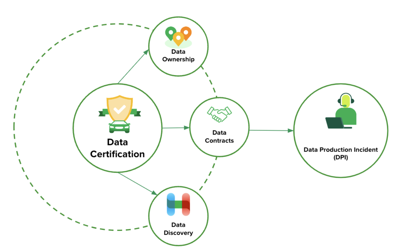
Figure 1: Concept of data certification
To achieve widespread data certification, we focused on several key enablers:
Ownership: Establishing decentralised ownership and accountability is fundamental and non-trivial. We clearly identified teams which we call Data Domains, individuals responsible as Business Data Owners (BDOs), and Technical Data Owners (TDOs) for the upkeep, usability, documentation, and associated Scheduled Large Orders (SLOs) of each data product. This step was bootstrapped by leveraging the identification of the data asset creator’s team. However, if the creator had changed teams or left the company, the initial mapping of Domain <> Data Asset needs to be reviewed by the Domain Leads.
Data contract: We introduced data contracts as formal agreements between data producers and consumers. These contracts define the schema, SLA guarantees (including freshness, completeness, and retention policies), notice period for changes, and communication channels for a data product. Data certification helps set clear expectations and ensures reliability across data pipelines.
Data operational excellence
To further enhance accountability and ensure adherence to data contracts, we implemented automated Data Production Incidents (DPIs) for breached contracts. When data quality tests are done on data availability, timeliness, consistency, completeness, accuracy, validity, or other reliability guarantees fail, a DPI ticket is automatically created and assigned to the TDO. This system aims to standardise and drive accountability in investigating and fixing issues related to reliability guarantees within Data Contracts. The goal is for teams to acknowledge and fix the root cause of the DPIs.
Operationalisation and outcomes
To drive the adoption of data certification and the principles of data mesh across Grab, we focused on the following north star metric: percentage of queries hitting certified assets (%). This metric serves as a direct indicator of the reusability and trust in our certified data products. It also helps teams prioritise their certification efforts towards the most frequently used tables. It essentially pushes every data team in two synergistic directions:
To certify their most used datasets.
To query only certified datasets as much as possible.
Operationalisation
The successful operationalisation of our data mesh and certification efforts relied on several key factors listed below:
Executive buy-in: Strong leadership support was crucial in driving this organisational change and emphasising the importance of data as a product.
Organisation-wide push with clear measurable reporting: We implemented an organisation-wide initiative with clearly defined goals and measurable targets for data certification. Progress is tracked and reported to ensure accountability and drive momentum.
Dashboard to guide Grabbers target most used tables: Dashboards and tooling likely within Hubble, provided visibility into data usage patterns, guiding teams to prioritise the certification of their most popular and impactful datasets.
Outcomes
As a result of these efforts, we have observed significant positive outcomes:
75% of Grab queries hitting certified assets: We achieved a significant milestone with 75% of Grab’s data queries now targeting certified assets. This indicates a strong adoption of certified data products and a growing trust in their reliability.
Active deprecation of assets: The focus on data ownership and the push for certification has also led to increased visibility into our data landscape, allowing us to identify and actively deprecate redundant and duplicated data assets. Deprecated tables increases 400% year over year (YoY). This not only improves efficiency but also reduces the complexity and cost of maintaining our data infrastructure.
Accelerated innovation and cross-domain reusability: Prior to data mesh, every team often resorted to building their own data sources which leads to lower quality outcomes and slower turn around time. Today, internet of things datasets (IoT) like weather data collected by one team can now be reused by another team to optimise marketplace decisions — a practical step toward a more connected data ecosystem.
Beyond these individual instances, we observe a convergence across Grab towards most used datasets, with the number of P80 datasets (the top 80% of Grab’s most used data) reducing by over 58% since the start of the campaign.
What’s next
While we have made significant strides in our data mesh journey, we recognise that this is an ongoing evolution. This progress wouldn’t be as smooth sailing without the platforms we build for data management and observability. In our next article, we will be delving into the enhancements for crucial tooling and platforms like Genchi (in-house data quality observational tool) and Hubble (metadata management platform, built on DataHub and Grab proprietary technology), which underpin our data mesh vision and enable greater data reliability and reusability.
Massive credits to Grab’s leadership, Mohan Krishnan and Nikhil Dwarakanath, as well as Data owners on driving this Grab-wide effort to build strong data foundations in Grab. Grab’s data mesh would not have been possible without the commitment of all data owners to certify and curate their data products.
Join us
Grab is a leading superapp in Southeast Asia, operating across the deliveries, mobility and digital financial services sectors. Serving over 800 cities in eight Southeast Asian countries, Grab enables millions of people everyday to order food or groceries, send packages, hail a ride or taxi, pay for online purchases or access services such as lending and insurance, all through a single app. Grab was founded in 2012 with the mission to drive Southeast Asia forward by creating economic empowerment for everyone. Grab strives to serve a triple bottom line – we aim to simultaneously deliver financial performance for our shareholders and have a positive social impact, which includes economic empowerment for millions of people in the region, while mitigating our environmental footprint.
Powered by technology and driven by heart, our mission is to drive Southeast Asia forward by creating economic empowerment for everyone. If this mission speaks to you, join our team today!
The Cloudflare Business Intelligence team manages a petabyte-scale data lake and ingests thousands of tables every day from many different sources. These include internal databases such as Postgres and ClickHouse, as well as external SaaS applications such as Salesforce. These tasks are often complex and tables may have hundreds of millions or billions of rows of new data each day. They are also business-critical for product decisions, growth plannings, and internal monitoring. In total, about 141 billion rows are ingested every day.
As Cloudflare has grown, the data has become ever larger and more complex. Our existing Extract Load Transform (ELT) solution could no longer meet our technical and business requirements. After evaluating other common ELT solutions, we concluded that their performance generally did not surpass our current system, either.
It became clear that we needed to build our own framework to cope with our unique requirements — and so Jetflow was born.
What we achieved
Over 100x efficiency improvement in GB-s:
Our longest running job with 19 billion rows was taking 48 hours using 300 GB of memory, and now completes in 5.5 hours using 4 GB of memory
We estimate that ingestion of 50 TB from Postgres via Jetflow could cost under $100 based on rates published by commercial cloud providers
>10x performance improvement:
Our largest dataset was ingesting 60-80,000 rows per second, this is now 2-5 million rows per second per database connection.
In addition, these numbers scale well with multiple database connections for some databases.
Extensibility:
The modular design makes it easy to extend and test. Today Jetflow works with ClickHouse, Postgres, Kafka, many different SaaS APIs, Google BigQuery and many others. It has continued to work well and remain flexible with the addition of new use cases.
How did we do this?
Requirements
The first step to designing our new framework had to be a clear understanding of the problems we were aiming to solve, with clear requirements to stop us creating new ones.
Performant & efficient
We needed to be able to move more data in less time as some ingestion jobs were taking ~24 hours, and our data will only grow. The data should be ingested in a streaming fashion and use less memory and compute resources than our existing solution.
Backwards compatible
Given the daily ingestion of thousands of tables, the chosen solution needed to allow for the migration of individual tables as needed. Due to our usage of Spark downstream and Spark’s limitations in merging desperate Parquet schemas, the chosen solution had to offer the flexibility to generate the precise schemas needed for each case to match legacy.
We also required seamless integration with our custom metadata system, used for dependency checks and job status information.
Ease of use
We want a configuration file that can be version-controlled, without introducing bottlenecks on repositories with many concurrent changes.
To increase accessibility for different roles within the team, another requirement was no-code (or configuration as code) in the vast majority of cases. Users should not have to worry about availability or translation of data types between source and target systems, or writing new code for each new ingestion. The configuration needed should also be minimal — for example, data schema should be inferred from the source system and not need to be supplied by the user.
Customizable
Striking a balance with the no-code requirement above, although we want a low bar of entry we also want to have the option to tune and override options if desired, with a flexible and optional configuration layer. For example, writing Parquet files is often more expensive than reading from the database, so we want to be able to allocate more resources and concurrency as needed.
Additionally, we wanted to allow for control over where the work is executed, with the ability to spin up concurrent workers in different threads, different containers, or on different machines. The execution of workers and communication of data was abstracted away with an interface, and different implementations can be written and injected, controlled via the job configuration.
Testable
We wanted a solution capable of running locally in a containerized environment, which would allow us to write tests for every stage of the pipeline. With “black box” solutions, testing often means validating the output after making a change, which is a slow feedback loop, risks not testing all edge cases as there isn’t good visibility of all code paths internally, and makes debugging issues painful.
Designing a flexible framework
To build a truly flexible framework, we broke the pipeline down into distinct stages, and then create a config layer to define the composition of the pipeline from these stages, and any configuration overrides. Every pipeline configuration that makes sense logically should execute correctly, and users should not be able to create pipeline configs that do not work.
Pipeline configuration
This led us to a design where we created stages which were classified according to the meaningfully different categories of:
Consumers
Transformers
Loaders
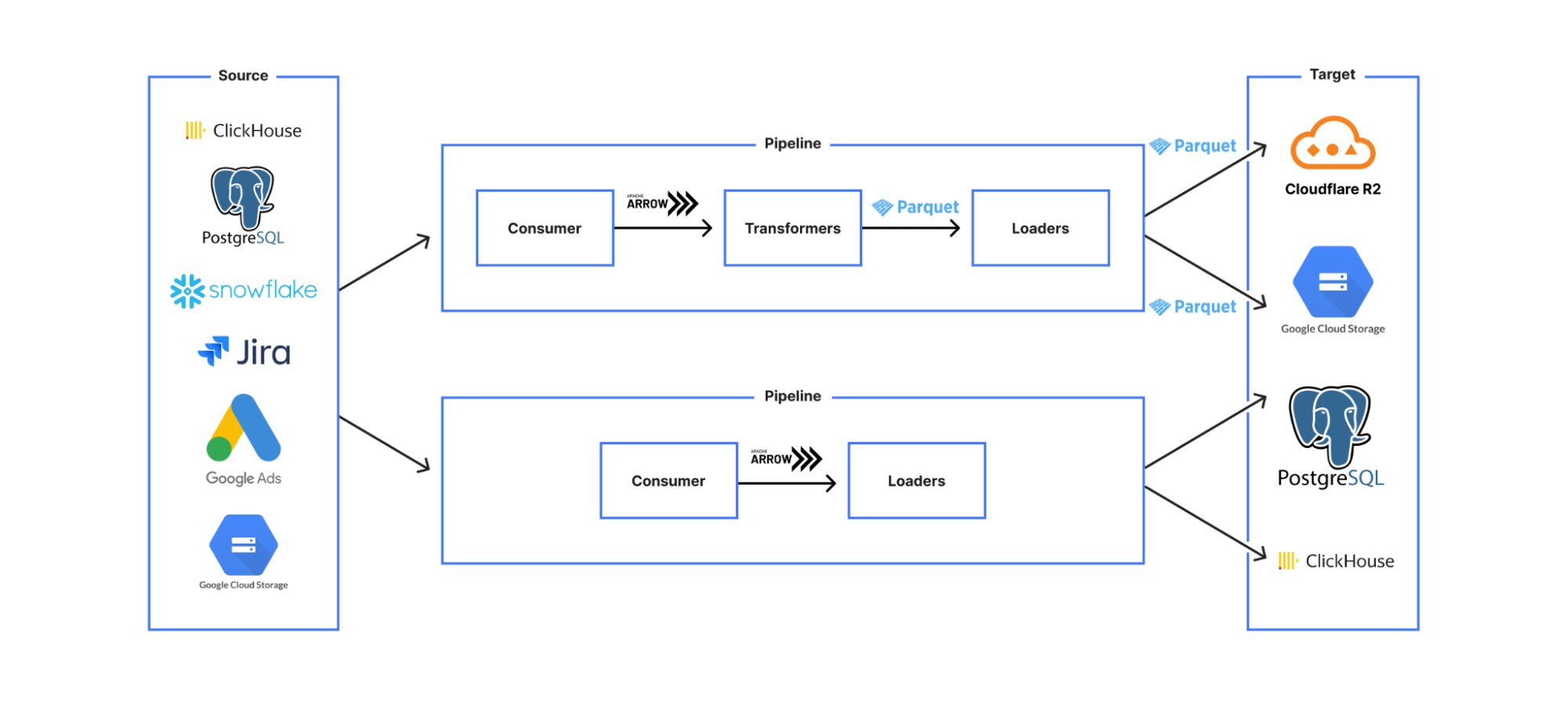
The pipeline was constructed via a YAML file that required a consumer, zero or more transformers, and at least one loader. Consumers create a data stream (via reading from the source system), Transformers (e.g. data transformations, validations) take a data stream input and output a data stream conforming to the same API so that they can be chained, and Loaders have the same data streaming interface, but are the stages with persistent effects — i.e. stages where data is saved to an external system.
This modular design means that each stage is independently testable, with shared behaviour (such as error handling and concurrency) inherited from shared base stages, significantly decreasing development time for new use cases and increasing confidence in code correctness.
Data divisions
Next, we designed a breakdown for the data that would allow the pipeline to be idempotent both on whole pipeline re-run and also on internal retry of any data partition due to transient error. We decided on a design that let us parallelize processing, while maintaining meaningful data divisions that allowed the pipeline to perform cleanups of data where required for a retry.
RunInstance: the least granular division, corresponding to a business unit for a single run of the pipeline (e.g. one month/day/hour of data).
Partition: a division of the RunInstance that allows each row to be allocated to a partition in a way that is deterministic and self-evident from the row data without external state, and is therefore idempotent on retry. (e.g. an accountId range, a 10-minute interval)
Batch: a division of the partition data that is non-deterministic and used only to break the data down into smaller chunks for streaming/parallel processing for faster processing with fewer resources. (e.g. 10k rows, 50 MB)
The options that the user configures in the consumer stage YAML both construct the query that is used to retrieve the data from the source system, and also encode the semantic meaning of this data division in a system agnostic way, so that later stages understand what this data represents — e.g. this partition contains the data for all accounts IDs 0-500. This means that we can do targeted data cleanup and avoid, for example, duplicate data entries if a single data partition is retried due to error.
Framework implementation
Standard internal state for stage compatibility
Our most common use case is something like read from a database, convert to Parquet format, and then save to object storage, with each of these steps being a separate stage. As more use cases were onboarded to Jetflow, we had to make sure that if someone wrote a new stage it would be compatible with the other stages. We don’t want to create a situation where new code needs to be written for every output format and target system, or you end up with a custom pipeline for every different use case.
The way we have solved this problem is by having our stage extractor class only allow output data in a single format. This means as long as any downstream stages support this format as in the input and output format they would be compatible with the rest of the pipeline. This seems obvious in retrospect, but internally was a painful learning experience, as we originally created a custom type system and struggled with stage interoperability.
For this internal format, we chose to use Arrow, an in-memory columnar data format. The key benefits of this format for us are:
Arrow ecosystem: Many data projects now support Arrow as an output format. This means when we write extractor stages for new data sources, it is often trivial to produce Arrow output.
No serialisation overhead: This makes it easy to move Arrow data between machines and even programming languages with minimum overhead. Jetflow was designed from the start to have the flexibility to be able to run in a wide range of systems via a job controller interface, so this efficiency in data transmission means there’s minimal compromise on performance when creating distributed implementations.
Reserve memory in large fixed-size batches to avoid memory allocations: As Go is a garbage collected (GC) language and GC cycle times are affected mostly by the number of objects rather than the sizes of those objects, fewer heap objects reduces CPU time spent garbage collecting significantly, even if the total size is the same. As the number of objects to scan, and possibly collect, during a GC cycle increases with the number of allocations, if we have 8192 rows with 10 columns each, Arrow would only require us to do 10 allocations versus the 8192 allocations of most drivers that allocate on a row by row basis, meaning fewer objects and lower GC cycle times with Arrow.
Converting rows to columns
Another important performance optimization was reducing the number of conversion steps that happen when reading and processing data. Most data ingestion frameworks internally represent data as rows. In our case, we are mostly writing data in Parquet format, which is column based. When reading data from column-based sources (e.g. ClickHouse, where most drivers receive RowBinary format), converting into row-based memory representations for the specific language implementation is inefficient. This is then converted again from rows to columns to write Parquet files. These conversions result in a significant performance impact.
Jetflow instead reads data from column-based sources in columnar formats (e.g. for ClickHouse-native Block format) and then copies this data into Arrow column format. Parquet files are then written directly from Arrow columns. The simplification of this process improves performance.
Writing each pipelines stage
Case study: ClickHouse
When testing an initial version of Jetflow, we discoveredthat due to the architecture of ClickHouse, using additional connections would not be of any benefit, since ClickHouse was reading faster than we were receiving data. It should then be possible, with a more optimized database driver, to take better advantage of that single connection to read a much larger number of rows per second, without needing additional connections.
Initially, a custom database driver was written for ClickHouse, but we ended up switching to the excellent ch-go low level library, which directly reads Blocks from ClickHouse in a columnar format. This had a dramatic effect on performance in comparison to the standard Go driver. Combined with the framework optimisations above, we now ingest millions of rows per second with a single ClickHouse connection.
A valuable lesson learned is that as with any software, tradeoffs are often made for the sake of convenience or a common use case that may not match your own. Most database drivers tend not to be optimized for reading large batches of rows, and have high per-row overhead.
Case study: Postgres
For Postgres, we use the excellent jackc/pgx driver, but instead of using the database/sql Scan interface, we directly receive the raw bytes for each row and use the jackc/pgx internal scan functions for each Postgres OID (Object Identifier) type.
The database/sql Scan interface in Go uses reflection to understand the type passed to the function and then also uses reflection to set each field with the column value received from Postgres. In typical scenarios, this is fast enough and easy to use, but falls short for our use cases in terms of performance. The jackc/pgx driver reuses the row bytes produced each time the next Postgres row is requested, resulting in zero allocations per row. This allows us to write high-performance, low-allocation code within Jetflow. With this design, we are able to achieve nearly 600,000 rows per second per Postgres connection for most tables, with very low memory usage.
Conclusion
As of early July 2025, the team ingests 77 billion records per day via Jetflow. The remaining jobs are in the process of being migrated to Jetflow, which will bring the total daily ingestion to 141 billion records. The framework has allowed us to ingest tables in cases that would not otherwise have been possible, and provided significant cost savings due to ingestions running for less time and with fewer resources.
In the future, we plan to open source the project, and if you are interested in joining our team to help develop tools like this, then open roles can be found at https://www.cloudflare.com/careers/jobs/.
The Integrity Data Platform (IDP) team decided to rewrite one of our heavy Queries Per Second (QPS) Golang microservices in Rust. It resulted in 70% infrastructure savings at a similar performance, but was not without its pitfalls. This article will elaborate on:
How we picked what to rewrite in Rust.
Approach taken to tackle the rewrite.
The pitfalls and speed bumps along the way.
Was it worthwhile?
Introduction
Grab is predominantly based on a microservice architecture, with the vast majority of microservices being hosted in a monorepo and written in Golang. It has served the company well so far, as the “simplicity” of Golang allows developers to ramp up and iterate quickly.
However, Rust has seen some gradual adoption across the company. Starting with a few minor CLIs, which then progressed to notable success with a Rust-based reverse proxy in Catwalk for model serving. Additionally, a growing community of Rust enthusiasts within the organisation has expressed interest in advocating for and expanding the adoption of Rust more proactively.
After achieving success with several projects on the ML platform and addressing concerns about Rust’s ability to handle traffic at scale, the next logical step was to assess the Return on Investment (ROI) of rewriting a Golang microservice in Rust.
Background
Rust has the reputation of being highly efficient yet poses a steep learning curve. Rust is often touted to perform close to C, doing away with garbage collection while remaining memory safe through strict compile checks and the borrow checker. It is loved by developers for having rich features like being multi-paradigm (supporting both functional and OOP style), having a rich type system, and doing away with nil pointers and errors.
However, regardless of how well regarded a certain language is in the industry, rewrites of any system should always be considered very carefully. When it comes to “legacy software”, there is a prevalent assumption that rewriting legacy software is a solution to eliminate technical debt and phase out legacy systems. The reality is often more nuanced.
Legacy code occurs when the developers who originally wrote the code are no longer working on the project. There are often business logic and edge-cases baked into complex legacy codebases of which the context has been lost over time. In practice, rewrites frequently take longer than anticipated and tend to reintroduce bugs and edge cases that must be identified and resolved all over again.
Rewriting vs refactoring has been written at length across the internet, you can read more about it here.
The trade-offs of rewriting need to be properly weighed and balanced. It must take into consideration:
How much engineering bandwidth goes into the rewrite?
What is the complexity of the rewrite?
What tangible benefits are brought about by the rewrite?
Rewriting a system solely for the purpose of “rewriting it in Rust” is not a strong enough business justification.
A legitimate concern was the steep learning curve of Rust, coupled with the risk of having only one team member proficient in the language, which would make its adoption unsustainable.
Therefore, we established a set of guidelines to follow when identifying a suitable system for a potential rewrite:
The system must be “simple” enough in functionality. For example, it has one or two main functionalities that can be rewritten in a reasonable amount of time and have its complexity constrained.
The system targeted should have large enough traffic such that cost savings brought about by adopting Rust is something tangible when balanced against the effort.
The members of the team must be comfortable and willing to pick up the language and achieve a certain level of familiarity to make maintaining the service sustainable.
Finding the right service
The ideal service should have a sufficiently large infrastructure footprint to justify the potential cost savings, while also being straightforward in functionality to minimise time spent on handling edge cases and complex business logic.
Looking across the stack of microservices in Integrity, Counter Service stands out. As its name implies, Counter Service is a service that “counts” and serves the counters for ML models and fraud rules. The original service has two primary functionalities:
Consuming from streams, counting events and writing to Scylla.
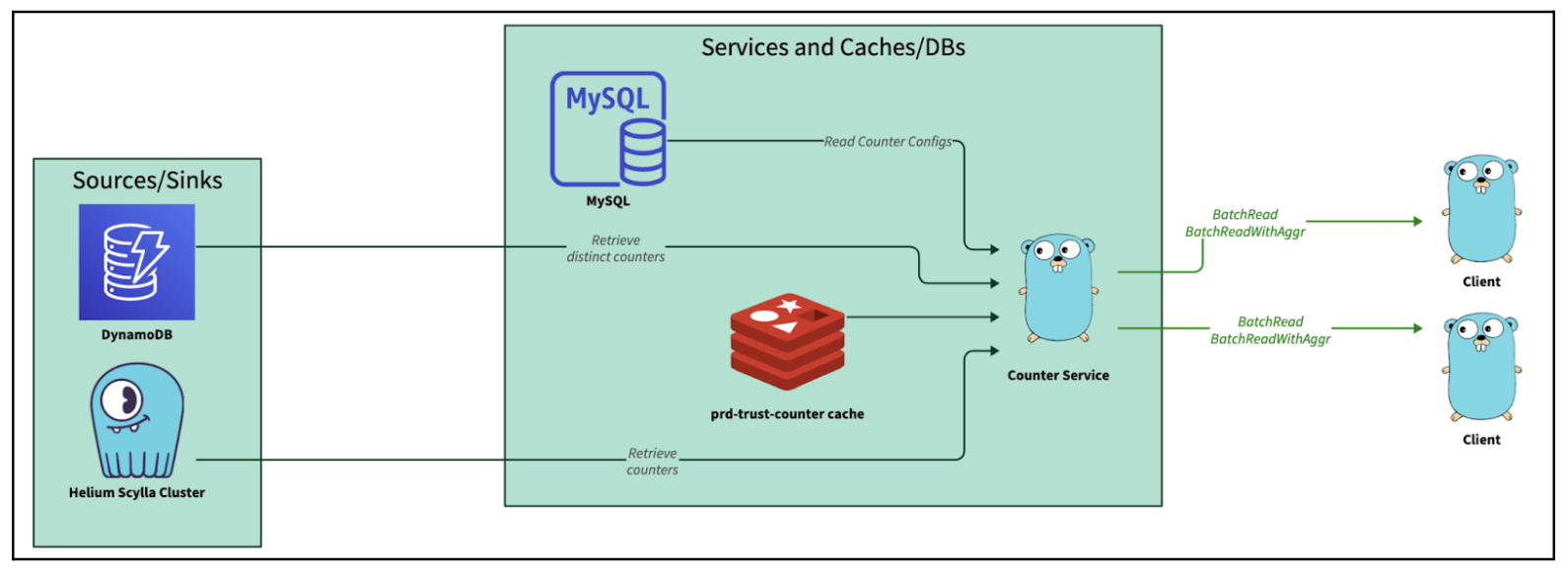
Exposing Google Remote Procedure Call (GRPC) endpoints to query from Scylla (and Redis) and return counts of events based on query keys. For example, BatchRead. BatchRead’s functionality of Counter Service serves up to tens of thousands of QPS at peak and is fairly constrained in functionality. Hence, it fulfilled our target criteria of being “simple” in functionality yet serving a large enough amount of traffic that justifies the ROI of a rewrite.
Figure 1: BatchRead flow of Counter Service, reading data from Scylla, DynamoDB, Redis, MySQL and serving the counters through GRPC.
Rewrite approach
There are a few ways to approach a rewrite in another language. One popular way is to convert your code line by line. If the languages are close enough, it might even be possible to programmatically convert your code like C2Rust.
We decided not to use such an approach for our rewrite. The major reason is that idiomatic Golang was not necessarily idiomatic Rust. We wanted to approach this rewrite with a fresh perspective and treat this as a true rewrite.
We treated the application like a black box, with the interfaces well defined, like GRPC endpoints and contracts. Similar to a function, you could call the API and get a deterministic result, and we had the data that was stored in Scylla.
Based on how we understood the application to work based on its specs and contract, we chose to rewrite the application logic from scratch to meet the API contract and to get as close as identical outputs from the new black box.
OSS library support
We started out by mapping out the key external dependencies and checking how well they were supported in the Rust ecosystem and in open source.
All the functionality we need is available through libraries in the Rust ecosystem. However, we found that some libraries are not particularly “popular,” as indicated by their relatively low number of GitHub stars.
The practical concern with using less “popular” libraries is the risk of limited community support or potential abandonment over time. That said, if an “unpopular” library is officially maintained by the associated open-source project—for instance, the Scylla driver has only about 500 stars but is officially provided by the Scylla project—we would need to ensure confidence that it will continue to receive active support.
Out of the list of libraries above, the “unpopular” and unofficial libraries can be narrowed down to two libraries:
Datadog – Cadence
Redis – Fred
For Datadog, there is no “official” Datadog Rust client. Yet, we picked Cadence as the API looked intuitive and the features we needed were already supported.
In regards to Redis, after testing it, we discovered that the support was not up to par with our requirements. We then opted for a newer and less popular library, fred.rs that seemed to be actively being developed by the community.
Company specific internal libraries
With the vast majority of microservices being written in Golang, most internal libraries are also written in Golang. Opting to rewrite a service in Rust means we are not able to use these internal libraries.
Examples include:
An internal configuration library that utilises Go Templates to template configurations for different environments (staging and production).
The internal configuration library has its own wrappers and injectors to pull and render secrets.
To overcome this gap and re-use Go Templates and configuration language, we decided to write a simple wrapper and parser using the nom parser combinator to parse the templates and render the config.
Nom poses a steep learning curve. But once familiarised, it is flexible and performant enough to build an equivalent to the internal library. Parser combinators are an interesting subset of tooling that allows you to create some fairly elegant parsers.
Road bumps
The borrow checker
One of the most striking paradigm shifts for developers transitioning to Rust is adapting to the strict rules of the borrow checker, which enforces that variables cannot be reused multiple times unless explicitly cloned or borrowed.
Interestingly, the borrow checker was not the biggest hurdle for new developers. The key is to avoid introducing lifetimes too early in the development process, as this can lead to premature code optimisation.
In many cases, adding a few clones (and occasionally Arcs) can help new developers get up to speed and iterate more quickly during development. The resulting code is usually “fast” enough for initial purposes. After that, the code can be revisited to eliminate unnecessary clones for improved performance. An efficient approach to this can be taken by using Flamegraph to profile your code and identify memory allocation bottlenecks.
Async gotchas
When rewriting Golang logic in Rust, there are fundamental differences in how they treat concurrency and parallelism.
One of Golang’s most remarkable strengths is its ability to deliver high-performance concurrency while preserving simplicity.
There are two fundamental approaches to concurrency in programming languages, namely:
Preemptive scheduling (stackful coroutines).
Cooperative scheduling (stackless coroutines).
Preemptive vs cooperative scheduling is an in-depth topic with the gist of it being, Golang uses preemptive scheduling and each “Goroutine” has a stack that needs a runtime. The Golang scheduler has the power to “preempt” and “freeze” functions and switch to another stack like stackful coroutine. This is a gross oversimplification of the nuances. For more details, this is a good introduction to the topic.
Rust opts for cooperative scheduling whereby it has no runtime and each coroutine does not maintain a stack. Hence, it has no ability to “freeze” a function and swap context. This allows Rust to be more efficient in terms of memory and resources, as it maintains a state machine. However, the consequence is that this moves the complexity up the stack to the programming language itself. Similar to Javascript, functions are “coloured”, and the developer has to explicitly annotate their functions to be async or sync. Await points need to be explicitly called and control needs to be “yielded” (i.e. cooperative and stackless) so the Rust program knows when it is allowed to stop and swap between coroutines. To read more on this, refer to this and this article for the history of async Rust.
Needing to annotate a function is a classic complaint that is addressed in the article “What Colour is Your Function” that highlights developers’ responsibility to explicitly colour their function and consciously think about blocking vs non-blocking code.
Contrast this with Golang, where you simply need to add the go keyword without thinking about which code might block the execution and use channels to communicate across Goroutines. Golang allows the developer to achieve high performance without much cognitive overhead.
This is especially important for developers new to Rust. As the lack of experience in async and blocking code can be somewhat of a footgun. In the initial rewrite of Rust, we made an amateur mistake of using a synchronous Redis function to call the Redis cache. It resulted in the application performing poorly until we corrected it with the non-blocking asynchronous version using the Fred redis library.
Impact
Following the eventful process of rewriting the service from the ground up in Rust, the outcomes proved to be quite intriguing.
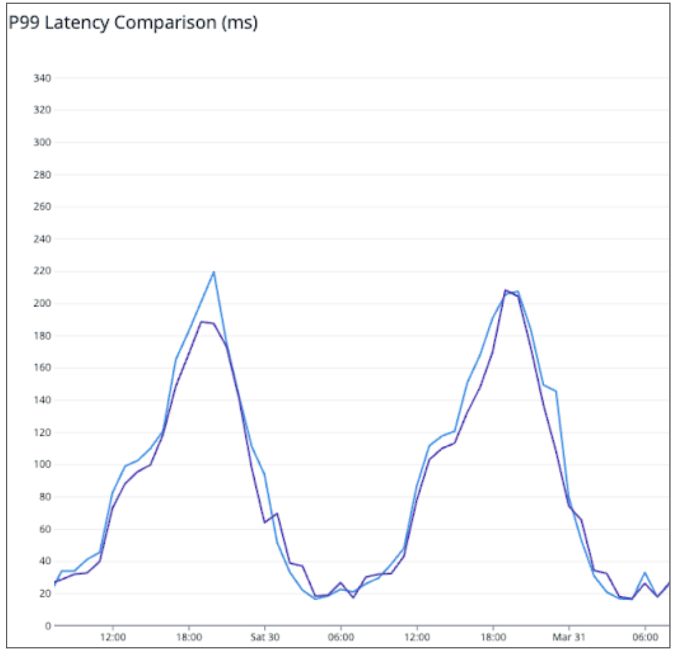
Shadowing traffic to both services as seen in Figure 2, the P99 latency is similar (or perhaps even slightly worse) in the Rust service compared to the original Golang one.
Figure 2: P99 latency comparison between the Golang service (purple) and Rust service (blue).
Normalising the QPS and resource consumption, we see from Table 2 that Rust consumes ~20% of the resources of the original Golang application, resulting in 5x savings in terms of resource consumption.
Table 2: Comparison of resource consumption between Rust and Golang service.
Service
Indicative QPS
Resources
Original Golang Service
1,000
20 Cores
New Rust Service
1,000
4.5 Cores
Learnings and conclusion
The outcomes and insights from this rewrite have been eye-opening, debunking certain myths while also validating others.
Myth 1: Rust is blazingly fast! Faster than Golang!
Verdict: Disproved.
Golang is “fast enough” for most use cases. It’s a mature language built with concurrency at its core, and it performs exceptionally well in its intended domain. While Rust can outperform Golang due to its higher performance ceiling and finer-grained control, rewriting a Golang service in Rust solely for performance improvements is unlikely to yield significant benefits.
Myth 2: Rust is more efficient than Golang
Verdict: True.
Rewriting a Golang service in Rust will probably give you 50% savings in compute. Rust does fulfill its promise of being memory safe without garbage collection, allowing it to be one of the more efficient languages out there. This is in line with other discoveries in the market.
Myth 3: The learning curve of Rust is too high
Verdict: It depends.
Pure synchronous Rust is fine. As long as you don’t overcomplicate the code and only clone what is needed, it is mostly true. The language is easy enough to pick up for most experienced developers. Even with cloning sprinkled in, the code is usually “fast enough”. The compiler is a good teacher, the compiler error messages are amazing, and if your code compiles, it probably works. Also, the Clippy linter is amazing.
However, introducing async can be challenging. Async is something quite different from what you would encounter in other languages like Go. Improper use of blocking code in async code can result in nuanced bugs that can catch inexperienced Rust developers off-guard.
Evaluating the worth of the rewrite
Yes, the effort was worth it for this service. The trade-off between development effort spent and the cost savings were justified.
As a side effect, the service is 80% cheaper and probably more bug free, as Rust eliminates a class of common Golang errors like Null pointers and concurrent map writes by virtue of the design of the language. If your code compiles, you usually have the confidence that it will work as you expect due to the language being more explicit.
Would we encourage choosing Rust over Golang for new microservices? Absolutely, as the resulting service is likely to be at least 50% more efficient than its Go counterpart. However, this decision presents an important and exciting opportunity for management and leaders to invest in empowering their engineers by equipping them with the skills to master Rust’s unique concepts, such as Async and Lifetimes. While the initial development pace might be slower as the team builds proficiency, this investment can unlock long-term benefits. Once the workforce is skilled in Rust, development speed should align with expectations, and the resulting systems are likely to be more stable and secure, thanks to Rust’s inherent safety features.
Join us
Grab is a leading superapp in Southeast Asia, operating across the deliveries, mobility and digital financial services sectors. Serving over 800 cities in eight Southeast Asian countries, Grab enables millions of people everyday to order food or groceries, send packages, hail a ride or taxi, pay for online purchases or access services such as lending and insurance, all through a single app. Grab was founded in 2012 with the mission to drive Southeast Asia forward by creating economic empowerment for everyone. Grab strives to serve a triple bottom line – we aim to simultaneously deliver financial performance for our shareholders and have a positive social impact, which includes economic empowerment for millions of people in the region, while mitigating our environmental footprint.
Powered by technology and driven by heart, our mission is to drive Southeast Asia forward by creating economic empowerment for everyone. If this mission speaks to you, join our team today!
Imagine scrolling through Netflix, where each movie poster or promotional banner competes for your attention. Every image you hover over isn’t just a visual placeholder; it’s a critical data point that fuels our sophisticated personalization engine. At Netflix, we call these images ‘impressions,’ and they play a pivotal role in transforming your interaction from simple browsing into an immersive binge-watching experience, all tailored to your unique tastes.
Capturing these moments and turning them into a personalized journey is no simple feat. It requires a state-of-the-art system that can track and process these impressions while maintaining a detailed history of each profile’s exposure. This nuanced integration of data and technology empowers us to offer bespoke content recommendations.
In this multi-part blog series, we take you behind the scenes of our system that processes billions of impressions daily. We will explore the challenges we encounter and unveil how we are building a resilient solution that transforms these client-side impressions into a personalized content discovery experience for every Netflix viewer.
Impressions on homepage
Why do we need impression history?
Enhanced Personalization
To tailor recommendations more effectively, it’s crucial to track what content a user has already encountered. Having impression history helps us achieve this by allowing us to identify content that has been displayed on the homepage but not engaged with, helping us deliver fresh, engaging recommendations.
Frequency Capping
By maintaining a history of impressions, we can implement frequency capping to prevent over-exposure to the same content. This ensures users aren’t repeatedly shown identical options, keeping the viewing experience vibrant and reducing the risk of frustration or disengagement.
Highlighting New Releases
For new content, impression history helps us monitor initial user interactions and adjust our merchandising efforts accordingly. We can experiment with different content placements or promotional strategies to boost visibility and engagement.
Analytical Insights
Additionally, impression history offers insightful information for addressing a number of platform-related analytics queries. Analyzing impression history, for example, might help determine how well a specific row on the home page is functioning or assess the effectiveness of a merchandising strategy.
Architecture Overview
The first pivotal step in managing impressions begins with the creation of a Source-of-Truth (SOT) dataset. This foundational dataset is essential, as it supports various downstream workflows and enables a multitude of use cases.
Collecting Raw Impression Events
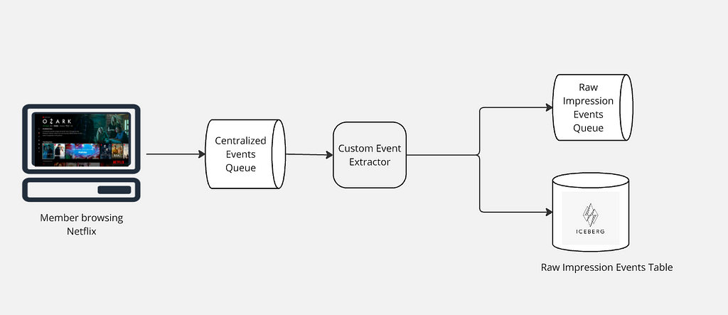
As Netflix members explore our platform, their interactions with the user interface spark a vast array of raw events. These events are promptly relayed from the client side to our servers, entering a centralized event processing queue. This queue ensures we are consistently capturing raw events from our global user base.
After raw events are collected into a centralized queue, a custom event extractor processes this data to identify and extract all impression events. These extracted events are then routed to an Apache Kafka topic for immediate processing needs and simultaneously stored in an Apache Iceberg table for long-term retention and historical analysis. This dual-path approach leverages Kafka’s capability for low-latency streaming and Iceberg’s efficient management of large-scale, immutable datasets, ensuring both real-time responsiveness and comprehensive historical data availability.
Collecting raw impression events
Filtering & Enriching Raw Impressions
Once the raw impression events are queued, a stateless Apache Flink job takes charge, meticulously processing this data. It filters out any invalid entries and enriches the valid ones with additional metadata, such as show or movie title details, and the specific page and row location where each impression was presented to users. This refined output is then structured using an Avro schema, establishing a definitive source of truth for Netflix’s impression data. The enriched data is seamlessly accessible for both real-time applications via Kafka and historical analysis through storage in an Apache Iceberg table. This dual availability ensures immediate processing capabilities alongside comprehensive long-term data retention.
Impression Source-of-Truth architecture
Ensuring High Quality Impressions
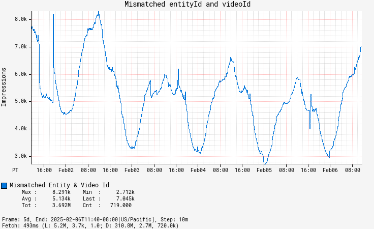
Maintaining the highest quality of impressions is a top priority. We accomplish this by gathering detailed column-level metrics that offer insights into the state and quality of each impression. These metrics include everything from validating identifiers to checking that essential columns are properly filled. The data collected feeds into a comprehensive quality dashboard and supports a tiered threshold-based alerting system. These alerts promptly notify us of any potential issues, enabling us to swiftly address regressions. Additionally, while enriching the data, we ensure that all columns are in agreement with each other, offering in-place corrections wherever possible to deliver accurate data.
Dashboard showing mismatch count between two columns- entityId and videoId
Configuration
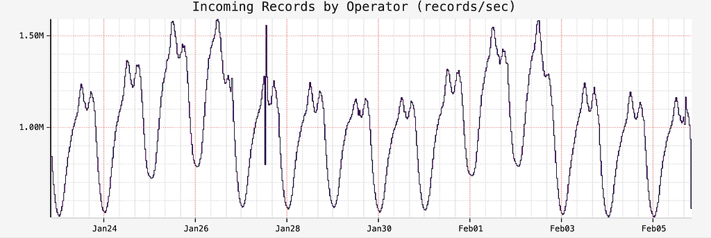
We handle a staggering volume of 1 to 1.5 million impression events globally every second, with each event approximately 1.2KB in size. To efficiently process this massive influx in real-time, we employ Apache Flink for its low-latency stream processing capabilities, which seamlessly integrates both batch and stream processing to facilitate efficient backfilling of historical data and ensure consistency across real-time and historical analyses. Our Flink configuration includes 8 task managers per region, each equipped with 8 CPU cores and 32GB of memory, operating at a parallelism of 48, allowing us to handle the necessary scale and speed for seamless performance delivery. The Flink job’s sink is equipped with a data mesh connector, as detailed in our Data Mesh platform which has two outputs: Kafka and Iceberg. This setup allows for efficient streaming of real-time data through Kafka and the preservation of historical data in Iceberg, providing a comprehensive and flexible data processing and storage solution.
Raw impressions records per second
We utilize the ‘island model’ for deploying our Flink jobs, where all dependencies for a given application reside within a single region. This approach ensures high availability by isolating regions, so if one becomes degraded, others remain unaffected, allowing traffic to be shifted between regions to maintain service continuity. Thus, all data in one region is processed by the Flink job deployed within that region.
Future Work
Addressing the Challenge of Unschematized Events
Allowing raw events to land on our centralized processing queue unschematized offers significant flexibility, but it also introduces challenges. Without a defined schema, it can be difficult to determine whether missing data was intentional or due to a logging error. We are investigating solutions to introduce schema management that maintains flexibility while providing clarity.
Automating Performance Tuning with Autoscalers
Tuning the performance of our Apache Flink jobs is currently a manual process. The next step is to integrate with autoscalers, which can dynamically adjust resources based on workload demands. This integration will not only optimize performance but also ensure more efficient resource utilization.
Improving Data Quality Alerts
Right now, there’s a lot of business rules dictating when a data quality alert needs to be fired. This leads to a lot of false positives that require manual judgement. A lot of times it is difficult to track changes leading to regression due to inadequate data lineage information. We are investing in building a comprehensive data quality platform that more intelligently identifies anomalies in our impression stream, keeps track of data lineage and data governance, and also, generates alerts notifying producers of any regressions. This approach will enhance efficiency, reduce manual oversight, and ensure a higher standard of data integrity.
Conclusion
Creating a reliable source of truth for impressions is a complex but essential task that enhances personalization and discovery experience. Stay tuned for the next part of this series, where we’ll delve into how we use this SOT dataset to create a microservice that provides impression histories. We invite you to share your thoughts in the comments and continue with us on this journey of discovering impressions.
Acknowledgments
We are genuinely grateful to our amazing colleagues whose contributions were essential to the success of Impressions: Julian Jaffe, Bryan Keller, Yun Wang, Brandon Bremen, Kyle Alford, Ron Brown and Shriya Arora.
Cloudflare’s network provides an enormous array of services to our customers. We collect and deliver associated data to customers in the form of event logs and aggregated analytics. As of December 2024, our data pipeline is ingesting up to 706M events per second generated by Cloudflare’s services, and that represents 100x growth since our 2018 data pipeline blog post.
At peak, we are moving 107 GiB/s of compressed data, either pushing it directly to customers or subjecting it to additional queueing and batching.
All of these data streams power things like Logs, Analytics, and billing, as well as other products, such as training machine learning models for bot detection. This blog post is focused on techniques we use to efficiently and accurately deal with the high volume of data we ingest for our Analytics products. A previous blog post provides a deeper dive into the data pipeline for Logs.
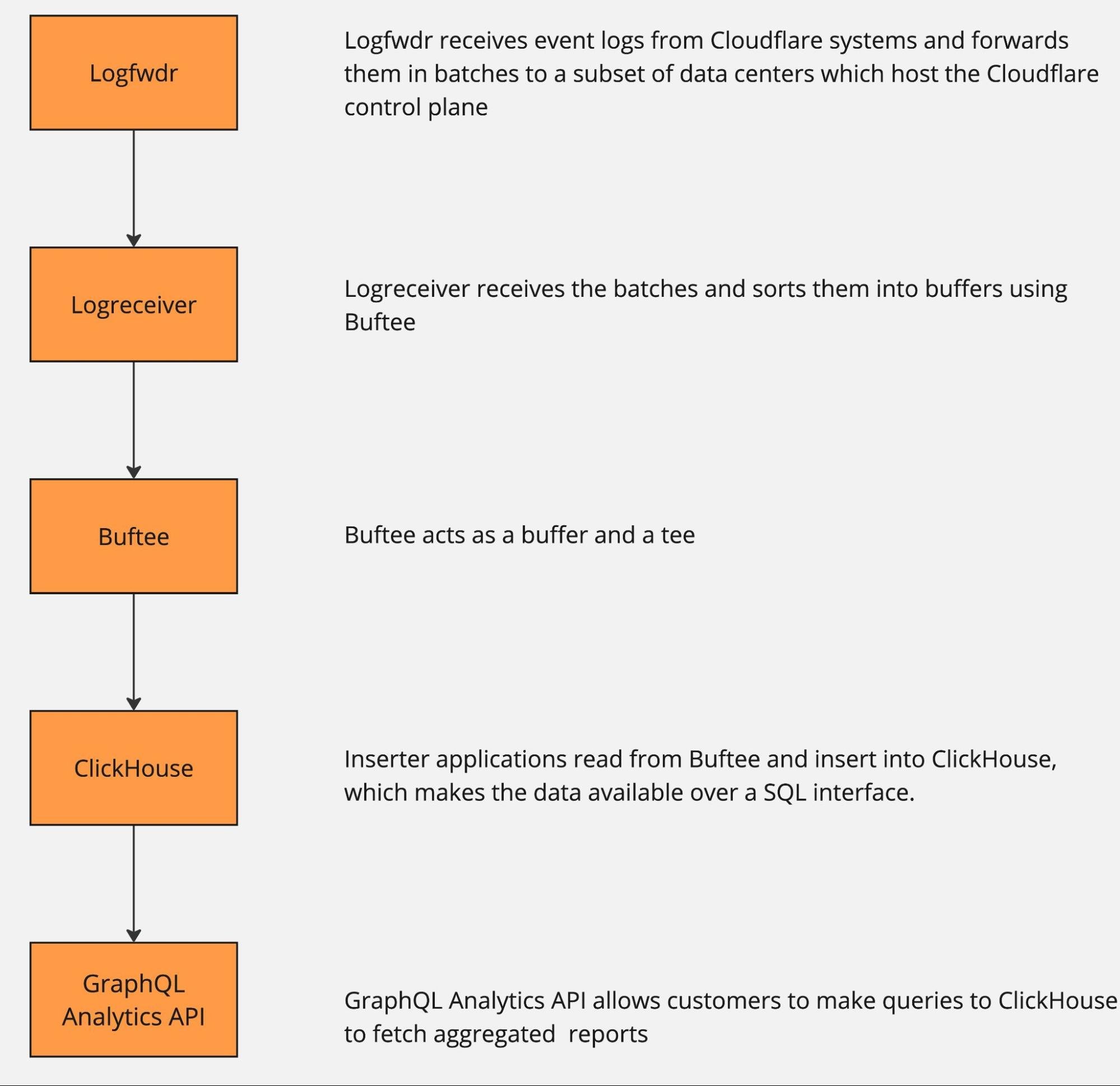
The pipeline can be roughly described by the following diagram.
The data pipeline has multiple stages, and each can and will naturally break or slow down because of hardware failures or misconfiguration. And when that happens, there is just too much data to be able to buffer it all for very long. Eventually some will get dropped, causing gaps in analytics and a degraded product experience unless proper mitigations are in place.
Dropping data to retain information
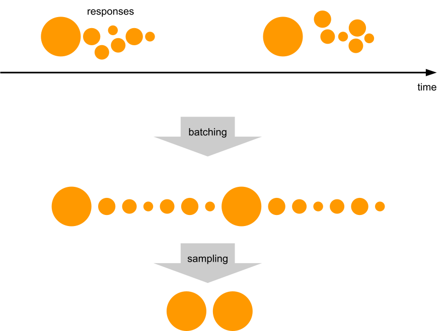
How does one retain valuable information from more than half a billion events per second, when some must be dropped? Drop it in a controlled way, by downsampling.
Here is a visual analogy showing the difference between uncontrolled data loss and downsampling. In both cases the same number of pixels were delivered. One is a higher resolution view of just a small portion of a popular painting, while the other shows the full painting, albeit blurry and highly pixelated.
As we noted above, any point in the pipeline can fail, so we want the ability to downsample at any point as needed. Some services proactively downsample data at the source before it even hits Logfwdr. This makes the information extracted from that data a little bit blurry, but much more useful than what otherwise would be delivered: random chunks of the original with gaps in between, or even nothing at all. The amount of “blur” is outside our control (we make our best effort to deliver full data), but there is a robust way to estimate it, as discussed in the next section.
Logfwdr can decide to downsample data sitting in the buffer when it overflows. Logfwdr handles many data streams at once, so we need to prioritize them by assigning each data stream a weight and then applying max-min fairness to better utilize the buffer. It allows each data stream to store as much as it needs, as long as the whole buffer is not saturated. Once it is saturated, streams divide it fairly according to their weighted size.
In our implementation (Go), each data stream is driven by a goroutine, and they cooperate via channels. They consult a single tracker object every time they allocate and deallocate memory. The tracker uses a max-heap to always know who the heaviest participant is and what the total usage is. Whenever the total usage goes over the limit, the tracker repeatedly sends the “please shed some load” signal to the heaviest participant, until the usage is again under the limit.
The effect of this is that healthy streams, which buffer a tiny amount, allocate whatever they need without losses. But any lagging streams split the remaining memory allowance fairly.
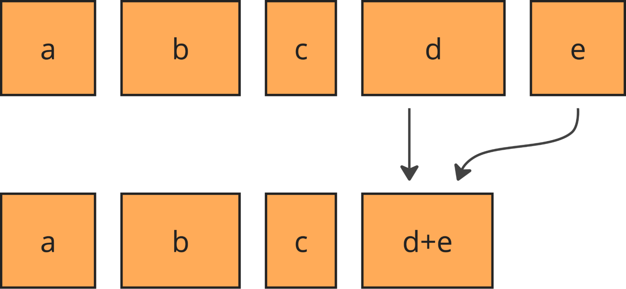
We downsample more or less uniformly, by always taking some of the least downsampled batches from the buffer (using min-heap to find those) and merging them together upon downsampling.
Merging keeps the batches roughly the same size and their number under control.
Downsampling is cheap, but since data in the buffer is compressed, it causes recompression, which is the single most expensive thing we do to the data. But using extra CPU time is the last thing you want to do when the system is under heavy load! We compensate for the recompression costs by starting to downsample the fresh data as well (before it gets compressed for the first time) whenever the stream is in the “shed the load” state.
We called this approach “bottomless buffers”, because you can squeeze effectively infinite amounts of data in there, and it will just automatically be thinned out. Bottomless buffers resemble reservoir sampling, where the buffer is the reservoir and the population comes as the input stream. But there are some differences. First is that in our pipeline the input stream of data never ends, while reservoir sampling assumes it ends to finalize the sample. Secondly, the resulting sample also never ends.
Let’s look at the next stage in the pipeline: Logreceiver. It sits in front of a distributed queue. The purpose of logreceiver is to partition each stream of data by a key that makes it easier for Logpush, Analytics inserters, or some other process to consume.
Logreceiver proactively performs adaptive sampling of analytics. This improves the accuracy of analytics for small customers (receiving on the order of 10 events per day), while more aggressively downsampling large customers (millions of events per second). Logreceiver then pushes the same data at multiple resolutions (100%, 10%, 1%, etc.) into different topics in the distributed queue. This allows it to keep pushing something rather than nothing when the queue is overloaded, by just skipping writing the high-resolution samples of data.
The same goes for Inserters: they can skip reading or writing high-resolution data. The Analytics APIs can skip reading high resolution data. The analytical database might be unable to read high resolution data because of overload or degraded cluster state or because there is just too much to read (very wide time range or very large customer). Adaptively dropping to lower resolutions allows the APIs to return some results in all of those cases.
Extracting value from downsampled data
Okay, we have some downsampled data in the analytical database. It looks like the original data, but with some rows missing. How do we make sense of it? How do we know if the results can be trusted?
Let’s look at the math.
Since the amount of sampling can vary over time and between nodes in the distributed system, we need to store this information along with the data. With each event $x_i$ we store its sample interval, which is the reciprocal to its inclusion probability $\pi_i = \frac{1}{\text{sample interval}}$. For example, if we sample 1 in every 1,000 events, each of the events included in the resulting sample will have its $\pi_i = 0.001$, so the sample interval will be 1,000. When we further downsample that batch of data, the inclusion probabilities (and the sample intervals) multiply together: a 1 in 1,000 sample from a 1 in 1,000 sample is a 1 in 1,000,000 sample of the original population. The sample interval of an event can also be interpreted roughly as the number of original events that this event represents, so in the literature it is known as weight $w_i = \frac{1}{\pi_i}$.
We rely on the Horvitz-Thompson estimator (HT, paper) in order to derive analytics about $x_i$. It gives two estimates: the analytical estimate (e.g. the population total or size) and the estimate of the variance of that estimate. The latter enables us to figure out how accurate the results are by building confidence intervals. They define ranges that cover the true value with a given probability (confidence level). A typical confidence level is 0.95, at which a confidence interval (a, b) tells that you can be 95% sure the true SUM or COUNT is between a and b.
So far, we know how to use the HT estimator for doing SUM, COUNT, and AVG.
Given a sample of size $n$, consisting of values $x_i$ and their inclusion probabilities $\pi_i$, the HT estimator for the population total (i.e. SUM) would be
where $\pi_{ij}$ is the probability of both $i$-th and $j$-th events being sampled together.
We use Poisson sampling, where each event is subjected to an independent Bernoulli trial (“coin toss”) which determines whether the event becomes part of the sample. Since each trial is independent, we can equate $\pi_{ij} = \pi_i \pi_j$, which when plugged in the variance estimator above turns the right-hand sum to zero:
if we could, but the original population size $N$ is not known, it is not stored anywhere, and it is not even possible to store because of custom filtering at query time. Plugging $\widehat{C}$ instead of $N$ only partially works. It gives a valid estimator for the mean itself, but not for its variance, so the constructed confidence intervals are unusable.
In all cases the corresponding pair of estimates are used as the $\mu$ and $\sigma^2$ of the normal distribution (because of the central limit theorem), and then the bounds for the confidence interval (of confidence level ) are:
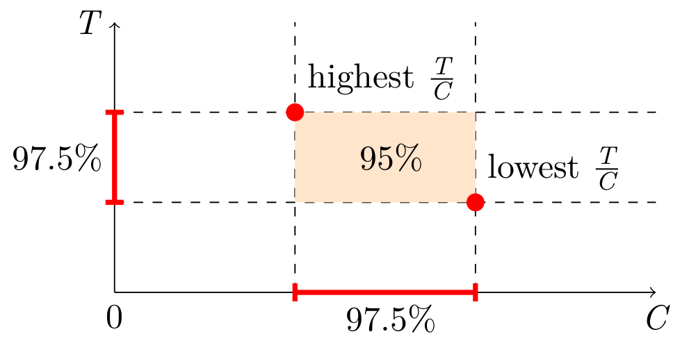
We do not know the N, but there is a workaround: simultaneous confidence intervals. Construct confidence intervals for SUM and COUNT independently, and then combine them into a confidence interval for AVG. This is known as the Bonferroni method. It requires generating wider (half the “inconfidence”) intervals for SUM and COUNT. Here is a simplified visual representation, but the actual estimator will have to take into account the possibility of the orange area going below zero.
In SQL, the estimators and confidence intervals look like this:
WITH sum(x * _sample_interval)                              AS t,
     sum(x * x * _sample_interval * (_sample_interval - 1)) AS vt,
     sum(_sample_interval)                                  AS c,
     sum(_sample_interval * (_sample_interval - 1))         AS vc,
     -- ClickHouse does not expose the erf⁻¹ function, so we precompute some magic numbers,
     -- (only for 95% confidence, will be different otherwise):
     --   1.959963984540054 = Φ⁻¹((1+0.950)/2) = √2 * erf⁻¹(0.950)
     --   2.241402727604945 = Φ⁻¹((1+0.975)/2) = √2 * erf⁻¹(0.975)
     1.959963984540054 * sqrt(vt) AS err950_t,
     1.959963984540054 * sqrt(vc) AS err950_c,
     2.241402727604945 * sqrt(vt) AS err975_t,
     2.241402727604945 * sqrt(vc) AS err975_c
SELECT t - err950_t AS lo_total,
       t            AS est_total,
       t + err950_t AS hi_total,
       c - err950_c AS lo_count,
       c            AS est_count,
       c + err950_c AS hi_count,
       (t - err975_t) / (c + err975_c) AS lo_average,
       t / c                           AS est_average,
       (t + err975_t) / (c - err975_c) AS hi_average
FROM ...
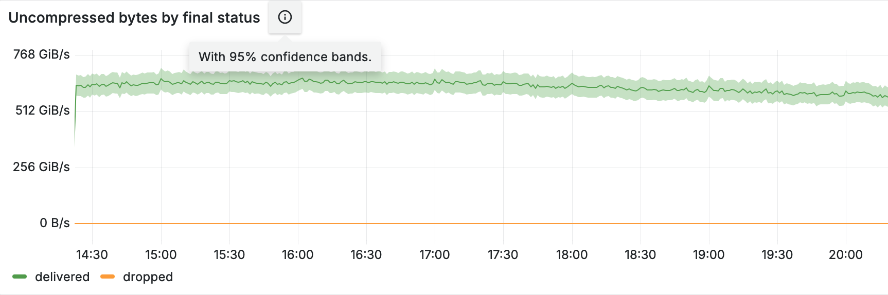
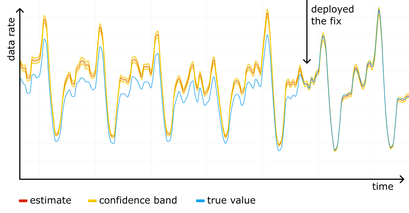
Construct a confidence interval for each timeslot on the timeseries, and you get a confidence band, clearly showing the accuracy of the analytics. The figure below shows an example of such a band in shading around the line.
Sampling is easy to screw up
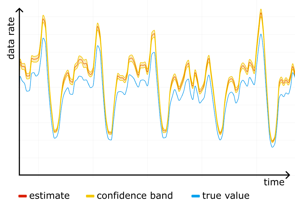
We started using confidence bands on our internal dashboards, and after a while noticed something scary: a systematic error! For one particular website the “total bytes served” estimate was higher than the true control value obtained from rollups, and the confidence bands were way off. See the figure below, where the true value (blue line) is outside the yellow confidence band at all times.
We checked the stored data for corruption, it was fine. We checked the math in the queries, it was fine. It was only after reading through the source code for all of the systems responsible for sampling that we found a candidate for the root cause.
We used simple random sampling everywhere, basically “tossing a coin” for each event, but in Logreceiver sampling was done differently. Instead of sampling randomly it would perform systematic sampling by picking events at equal intervals starting from the first one in the batch.
Why would that be a problem?
There are two reasons. The first is that we can no longer claim $\pi_{ij} = \pi_i \pi_j$, so the simplified variance estimator stops working and confidence intervals cannot be trusted. But even worse, the estimator for the total becomes biased. To understand why exactly, we wrote a short repro code in Python:
import itertools

def take_every(src, period):
    for i, x in enumerate(src):
    if i % period == 0:
        yield x

pattern = [10, 1, 1, 1, 1, 1]
sample_interval = 10 # bad if it has common factors with len(pattern)
true_mean = sum(pattern) / len(pattern)

orig = itertools.cycle(pattern)
sample_size = 10000
sample = itertools.islice(take_every(orig, sample_interval), sample_size)

sample_mean = sum(sample) / sample_size

print(f"{true_mean=} {sample_mean=}")
After playing with different values for pattern and sample_interval in the code above, we realized where the bias was coming from.
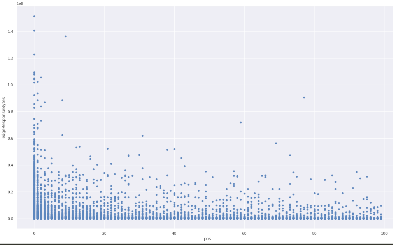
Imagine a person opening a huge generated HTML page with many small/cached resources, such as icons. The first response will be big, immediately followed by a burst of small responses. If the website is not visited that much, responses will tend to end up all together at the start of a batch in Logfwdr. Logreceiver does not cut batches, only concatenates them. The first response remains first, so it always gets picked and skews the estimate up.
We checked the hypothesis against the raw unsampled data that we happened to have because that particular website was also using one of the Logs products. We took all events in a given time range, and grouped them by cutting at gaps of at least one minute. In each group, we ranked all events by time and looked at the variable of interest (response size in bytes), and put it on a scatter plot against the rank inside the group.
A clear pattern! The first response is much more likely to be larger than average.
We fixed the issue by making Logreceiver shuffle the data before sampling. As we rolled out the fix, the estimation and the true value converged.
Now, after battle testing it for a while, we are confident the HT estimator is implemented properly and we are using the correct sampling process.
Using Cloudflare’s analytics APIs to query sampled data
We already power most of our analytics datasets with sampled data. For example, the Workers Analytics Engine exposes the sample interval in SQL, allowing our customers to build their own dashboards with confidence bands. In the GraphQL API, all of the data nodes that have “Adaptive” in their name are based on sampled data, and the sample interval is exposed as a field there as well, though it is not possible to build confidence intervals from that alone. We are working on exposing confidence intervals in the GraphQL API, and as an experiment have added them to the count and edgeResponseBytes (sum) fields on the httpRequestsAdaptiveGroups nodes. This is available under confidence(level: X).
The query above asks for the estimates and the 95% confidence intervals for SUM(edgeResponseBytes) and COUNT. The results will also show the sample size, which is good to know, as we rely on the central limit theorem to build the confidence intervals, thus small samples don’t work very well.
The response shows the estimated count is 96947, and we are 95% confident that the true count lies in the range 96874.24 to 97019.76. Similarly, the estimate and range for the sum of response bytes are provided.
The estimates are based on a sample size of 96294 rows, which is plenty of samples to calculate good confidence intervals.
Conclusion
We have discussed what kept our data pipeline scalable and resilient despite doubling in size every 1.5 years, how the math works, and how it is easy to mess up. We are constantly working on better ways to keep the data pipeline, and the products based on it, useful to our customers. If you are interested in doing things like that and want to help us build a better Internet, check out our careers page.
On November 14, 2024, Cloudflare experienced an incident which impacted the majority of customers using Cloudflare Logs. During the roughly 3.5 hours that these services were impacted, about 55% of the logs we normally send to customers were not sent and were lost. We’re very sorry this happened, and we are working to ensure that a similar issue doesn’t happen again.
This blog post explains what happened and what we’re doing to prevent recurrences. Also, the systems involved and the particular class of failure we experienced will hopefully be of interest to engineering teams beyond those specifically using these products.
Failures within systems at scale are inevitable, and it’s essential that subsystems protect themselves from failures in other parts of the larger system to prevent cascades. In this case, a misconfiguration in one part of the system caused a cascading overload in another part of the system, which was itself misconfigured. Had it been properly configured, it could have prevented the loss of logs.
Background
Cloudflare’s network is a globally distributed system enabling and supporting a wide variety of services. Every part of this system generates event logs which contain detailed metadata about what’s happening with our systems around the world. For example, an event log is generated for every request to Cloudflare’s CDN. Cloudflare Logs makes these event logs available to customers, who use them in a number of ways, including compliance, observability, and accounting.
On a typical day, Cloudflare sends about 4.5 trillion individual event logs to customers. Although this represents less than 10% of the over 50 trillion total customer event logs processed, it presents unique challenges of scale when building a reliable and fault-tolerant system.
System architecture
Cloudflare’s network is composed of tens of thousands of individual servers, network hardware components, and specialized software programs located in over 330 cities around the world. Although Cloudflare’s Edge Log Delivery product will send customers their event logs directly from each server, most customers opt not to do this because doing so will create significant complication and cost at the receiving end.
By analogy, imagine the postal service ringing your doorbell once for each letter instead of once for each packet of letters. With thousands or millions of letters each second, the number of separate transactions that would entail becomes prohibitive.
Fortunately, we also offer Logpush, which collects and pushes logs to customers in more predictable file sizes and which scales automatically with usage. In order to provide this feature several services work together to collect and push the logs, as illustrated in the diagram below:
Logfwdr
Logfwdr is an internal service written in Golang that accepts event logs from internal services running across Cloudflare’s global network and forwards them in batches to a service called Logreceiver. Logfwdr handles many different types of event logs, and one of its responsibilities is to determine which event logs should be forwarded and where they should be sent based on the type of event log, which customers it represents, and associated rules about where it should be processed. Configuration is provided to Logfwdr to enable it to make these determinations.
Logreceiver
Logreceiver (also written in Golang) accepts the batches of logs from across Cloudflare’s global network and further sorts them depending on the type of event and its purpose. For Cloudflare Logs, Logreceiver demultiplexes the batches into per-customer batches and forwards them to be buffered by Buftee. Currently, Logreceiver is handling about 45 PB (uncompressed) of customer event logs each day.
Buftee
It’s common for data pipelines to include a buffer. Producers and consumers of the data might be operating at different cadences, and parts of the pipeline will experience variances in how quickly they can process information. Using a buffer makes it easier to manage these situations, and helps to prevent data loss if downstream consumers are broken. It’s also convenient to have a buffer that supports multiple downstream consumers with different cadences (like the pipe fitting function of a tee.)
At Cloudflare, we use an internal system called Buftee (written in Golang) to support this combined function. Buftee is a highly distributed system which supports a large number of named “buffers”. It supports operating on named “prefixes” (collections of buffers) as well as multiple representations/resolutions of the same time-indexed dataset. Using Buftee makes it possible for Cloudflare to handle extremely high throughput very efficiently.
For Cloudflare Logs, Buftee provides buffers for each Logpush job, containing 100% of the logs generated by the zone or account referenced by each job. This means that failure to process one customer’s job will not affect progress on another customer’s job. Handling buffers in this way avoids “head of line” blocking and also enables us to encrypt and delete each customer’s data separately if needed.
Buftee typically handles over 1 million buffers globally. The following is a snapshot of the number of buffers managed by Buftee servers in the period just prior to the incident.
Logpush
Logpush is a Golang service which reads logs from Buftee buffers and pushes the results in batches to various destinations configured by customers. A batch could end up, for example, as a file in R2. Each job has a unique configuration, and only jobs that are active and configured will be pushed. Currently, we push over 600 million such batches each day.
What happened
On November 14, 2024, we made a change to support an additional dataset for Logpush. This required adding a new configuration to be provided to Logfwdr in order for it to know which customers’ logs to forward for this new stream. Every few minutes, a separate system re-generates the configuration used by Logfwdr to decide which logs need to be forwarded. A bug in this system resulted in a blank configuration being provided to Logfwdr.
This bug essentially informed Logfwdr that no customers had logs configured to be pushed. The team quickly noticed the mistake and reverted the change in under five minutes.
Unfortunately, this first mistake triggered a second, latent bug in Logfwdr itself. A failsafe introduced in the early days of this feature, when traffic was much lower, was configured to “fail open”. This failsafe was designed to protect against a situation when this specific Logfwdr configuration was unavailable (as in this case) by transmitting events for all customers instead of just those who had configured a Logpush job. This was intended to prevent the loss of logs at the expense of sending more logs than strictly necessary when individual hosts were prevented from getting the configuration due to intermittent networking errors, for example.
When this failsafe was first introduced, the potential list of customers was smaller than it is today. This small window of less than five minutes resulted in a massive spikein the number of customers whose logs were sent by Logfwdr.
Even given this massive overload, our systems would have continued to send logs if not for one additional problem. Remember that Buftee creates a separate buffer for each customer with their logs to be pushed. When Logfwdr began to send event logs for all customers, Buftee began to create buffers for each one as those logs arrived, and each buffer requires resources as well as the bookkeeping to maintain them. This massive increase, resulting in roughly 40 times more buffers, is not something we’ve provisioned Buftee clusters to handle. In the lead-up to impact, Buftee was managing 40 million buffers globally, as shown in the figure below.
A short temporary misconfiguration lasting just five minutes created a massive overload that took us several hours to fix and recover from. Because our backstops were not properly configured, the underlying systems became so overloaded that we could not interact with them normally. A full reset and restart was required.
Root causes
The bug in the Logfwdr configuration system was easy to fix, but it’s the type of bug that was likely to happen at some point. We had planned for it by designing the original “fail open” behavior. However, we neglected to regularly test that the broader system was capable of handling a fail open event.
The bigger failure was that Buftee became unresponsive. Buftee’s purpose is to be a safeguard against bugs like this one. A huge increase in the number of buffers is a failure mode that we had predicted, and had put mechanisms in Buftee to prevent this failure from cascading. Our failure in this case was that we had not configured these mechanisms. Had they been configured correctly, Buftee would not have been overwhelmed.
It’s like having a seatbelt in a car, yet not fastening it. The seatbelt is there to protect you in case of an accident but if you don’t actually buckle it up, it’s not going to do its job when you need it. Similarly, while we had the safeguard of Buftee in place, we hadn’t ‘buckled it up’ by configuring the necessary settings. We’re very sorry this happened and are taking steps to prevent a recurrence as described below.
Going forward
We’re creating alerts to ensure that these particular misconfigurations will be impossible to miss, and we are also addressing the specific bug and the associated tests that triggered this incident.
Just as importantly, we accept that mistakes and misconfigurations are inevitable. All our systems at Cloudflare need to respond to these predictably and gracefully. Currently, we conduct regular “cut tests” to ensure that these systems will cope with the loss of a datacenter or a network failure. In the future, we’ll also conduct regular “overload tests” to simulate the kind of cascade which happened in this incident to ensure that our production systems will handle them gracefully.
Logpush is a robust and flexible platform for customers who need to integrate their own logging and monitoring systems with Cloudflare. Different Logpush jobs can be deployed to support multiple destinations or, with filtering, multiple subsets of logs.
We are thrilled to announce that the Maestro source code is now open to the public! Please visit the Maestro GitHub repository to get started. If you find it useful, please give us a star.
What is Maestro
Maestro is a general-purpose, horizontally scalable workflow orchestrator designed to manage large-scale workflows such as data pipelines and machine learning model training pipelines. It oversees the entire lifecycle of a workflow, from start to finish, including retries, queuing, task distribution to compute engines, etc.. Users can package their business logic in various formats such as Docker images, notebooks, bash script, SQL, Python, and more. Unlike traditional workflow orchestrators that only support Directed Acyclic Graphs (DAGs), Maestro supports both acyclic and cyclic workflows and also includes multiple reusable patterns, including foreach loops, subworkflow, and conditional branch, etc.
Our Journey with Maestro
Since we first introduced Maestro in this blog post, we have successfully migrated hundreds of thousands of workflows to it on behalf of users with minimal interruption. The transition was seamless, and Maestro has met our design goals by handling our ever-growing workloads. Over the past year, we’ve seen a remarkable 87.5% increase in executed jobs. Maestro now launches thousands of workflow instances and runs half a million jobs daily on average, and has completed around 2 million jobs on particularly busy days.
Scalability and Versatility
Maestro is a fully managed workflow orchestrator that provides Workflow-as-a-Service to thousands of end users, applications, and services at Netflix. It supports a wide range of workflow use cases, including ETL pipelines, ML workflows, AB test pipelines, pipelines to move data between different storages, etc. Maestro’s horizontal scalability ensures it can manage both a large number of workflows and a large number of jobs within a single workflow.
At Netflix, workflows are intricately connected. Splitting them into smaller groups and managing them across different clusters adds unnecessary complexity and degrades the user experience. This approach also requires additional mechanisms to coordinate these fragmented workflows. Since Netflix’s data tables are housed in a single data warehouse, we believe a single orchestrator should handle all workflows accessing it.
Join us on this exciting journey by exploring the Maestro GitHub repository and contributing to its ongoing development. Your support and feedback are invaluable as we continue to improve the Maestro project.
Introducing Maestro
Netflix Maestro offers a comprehensive set of features designed to meet the diverse needs of both engineers and non-engineers. It includes the common functions and reusable patterns applicable to various use cases in a loosely coupled way.
A workflow definition is defined in a JSON format. Maestro combines user-supplied fields with those managed by Maestro to form a flexible and powerful orchestration definition. An example can be found in the Maestro repository wiki.
A Maestro workflow definition comprises two main sections: properties and versioned workflow including its metadata. Properties include author and owner information, and execution settings. Maestro preserves key properties across workflow versions, such as author and owner information, run strategy, and concurrency settings. This consistency simplifies management and aids in trouble-shootings. If the ownership of the current workflow changes, the new owner can claim the ownership of the workflows without creating a new workflow version. Users can also enable the triggering or alerting features for a given workflow over the properties.
Versioned workflow includes attributes like a unique identifier, name, description, tags, timeout settings, and criticality levels (low, medium, high) for prioritization. Each workflow change creates a new version, enabling tracking and easy reversion, with the active or the latest version used by default. A workflow consists of steps, which are the nodes in the workflow graph defined by users. Steps can represent jobs, another workflow using subworkflow step, or a loop using foreach step. Steps consist of unique identifiers, step types, tags, input and output step parameters, step dependencies, retry policies, and failure mode, step outputs, etc. Maestro supports configurable retry policies based on error types to enhance step resilience.
This high-level overview of Netflix Maestro’s workflow definition and properties highlights its flexibility to define complex workflows. Next, we dive into some of the useful features in the following sections.
Workflow Run Strategy
Users want to automate data pipelines while retaining control over the execution order. This is crucial when workflows cannot run in parallel or must halt current executions when new ones occur. Maestro uses predefined run strategies to decide whether a workflow instance should run or not. Here is the list of predefined run strategies Maestro offers.
Sequential Run Strategy This is the default strategy used by maestro, which runs workflows one at a time based on a First-In-First-Out (FIFO) order. With this run strategy, Maestro runs workflows in the order they are triggered. Note that an execution does not depend on the previous states. Once a workflow instance reaches one of the terminal states, whether succeeded or not, Maestro will start the next one in the queue.
Strict Sequential Run Strategy With this run strategy, Maestro will run workflows in the order they are triggered but block execution if there’s a blocking error in the workflow instance history. Newly triggered workflow instances are queued until the error is resolved by manually restarting the failed instances or marking the failed ones unblocked.
In the above example, run5 fails at 5AM, then later runs are queued but do not run. When someone manually marks run5 unblocked or restarts it, then the workflow execution will resume. This run strategy is useful for time insensitive but business critical workflows. This gives the workflow owners the option to review the failures at a later time and unblock the executions after verifying the correctness.
First-only Run Strategy With this run strategy, Maestro ensures that the running workflow is complete before queueing a new workflow instance. If a new workflow instance is queued while the current one is still running, Maestro will remove the queued instance. Maestro will execute a new workflow instance only if there is no workflow instance currently running, effectively turning off queuing with this run strategy. This approach helps to avoid idempotency issues by not queuing new workflow instances.
Last-only Run Strategy With this run strategy, Maestro ensures the running workflow is the latest triggered one and keeps only the last instance. If a new workflow instance is queued while there is an existing workflow instance already running, Maestro will stop the running instance and execute the newly triggered one. This is useful if a workflow is designed to always process the latest data, such as processing the latest snapshot of an entire table each time.
Parallel with Concurrency Limit Run Strategy With this run strategy, Maestro will run multiple triggered workflow instances in parallel, constrained by a predefined concurrency limit. This helps to fan out and distribute the execution, enabling the processing of large amounts of data within the time limit. A common use case for this strategy is for backfilling the old data.
Parameters and Expression Language Support
In Maestro, parameters play an important role. Maestro supports dynamic parameters with code injection, which is super useful and powerful. This feature significantly enhances the flexibility and dynamism of workflows, allowing using parameters to control execution logic and enable state sharing between workflows and their steps, as well as between upstream and downstream steps. Together with other Maestro features, it makes the defining of workflows dynamic and enables users to define parameterized workflows for complex use cases.
However, code injection introduces significant security and safety concerns. For example, users might unintentionally write an infinite loop that creates an array and appends items to it, eventually crashing the server with out-of-memory (OOM) issues. While one approach could be to ask users to embed the injected code within their business logic instead of the workflow definition, this would impose additional work on users and tightly couple their business logic with the workflow. In certain cases, this approach blocks users to design some complex parameterized workflows.
To mitigate these risks and assist users to build parameterized workflows, we developed our own customized expression language parser, a simple, secure, and safe expression language (SEL). SEL supports code injection while incorporating validations during syntax tree parsing to protect the system. It leverages the Java Security Manager to restrict access, ensuring a secure and controlled environment for code execution.
Simple, Secure, and Safe Expression Language (SEL) SEL is a homemade simple, secure, and safe expression language (SEL) to address the risks associated with code injection within Maestro parameterized workflows. It is a simple expression language and the grammar and syntax follow JLS (Java Language Specifications). SEL supports a subset of JLS, focusing on Maestro use cases. For example, it supports data types for all Maestro parameter types, raising errors, datetime handling, and many predefined utility methods. SEL also includes additional runtime checks, such as loop iteration limits, array size checks, object memory size limits and so on, to enhance security and reliability. For more details about SEL, please refer to the Maestro GitHub documentation.
Output Parameters To further enhance parameter support, Maestro allows for callable step execution, which returns output parameters from user execution back to the system. The output data is transmitted to Maestro via its REST API, ensuring that the step runtime does not have direct access to the Maestro database. This approach significantly reduces security concerns.
Parameterized Workflows Thanks to the powerful parameter support, users can easily create parameterized workflows in addition to static ones. Users enjoy defining parameterized workflows because they are easy to manage and troubleshoot while being powerful enough to solve complex use cases.
Static workflows are simple and easy to use but come with limitations. Often, users have to duplicate the same workflow multiple times to accommodate minor changes. Additionally, workflow and jobs cannot share the states without using parameters.
On the other hand, completely dynamic workflows can be challenging to manage and support. They are difficult to debug or troubleshoot and hard to be reused by others.
Parameterized workflows strike a balance by being initialized step by step at runtime based on user defined parameters. This approach provides great flexibility for users to control the execution at runtime while remaining easy to manage and understand.
As we described in the previous Maestro blog post, parameter support enables the creation of complex parameterized workflows, such as backfill data pipelines.
Workflow Execution Patterns
Maestro provides multiple useful building blocks that allow users to easily define dataflow patterns or other workflow patterns. It provides support for common patterns directly within the Maestro engine. Direct engine support not only enables us to optimize these patterns but also ensures a consistent approach to implementing them. Next, we will talk about the three major building blocks that Maestro provides.
Foreach Support In Maestro, the foreach pattern is modeled as a dedicated step within the original workflow definition. Each iteration of the foreach loop is internally treated as a separate workflow instance, which scales similarly as any other Maestro workflow based on the step executions (i.e. a sub-graph) defined within the foreach definition block. The execution of sub-graph within a foreach step is delegated to a separate workflow instance. Foreach step then monitors and collects the status of these foreach workflow instances, each managing the execution of a single iteration. For more details, please refer to our previous Maestro blog post.
The foreach pattern is frequently used to repeatedly run the same jobs with different parameters, such as data backfilling or machine learning model tuning. It would be tedious and time consuming to request users to explicitly define each iteration in the workflow definition (potentially hundreds of thousands of iterations). Additionally, users would need to create new workflows if the foreach range changes, further complicating the process.
Conditional Branch Support The conditional branch feature allows subsequent steps to run only if specific conditions in the upstream step are met. These conditions are defined using the SEL expression language, which is evaluated at runtime. Combined with other building blocks, users can build powerful workflows, e.g. doing some remediation if the audit check step fails and then run the job again.
Subworkflow Support The subworkflow feature allows a workflow step to run another workflow, enabling the sharing of common functions across multiple workflows. This effectively enables “workflow as a function” and allows users to build a graph of workflows. For example, we have observed complex workflows consisting of hundreds of subworkflows to process data across hundreds tables, where subworkflows are provided by multiple teams.
These patterns can be combined together to build composite patterns for complex workflow use cases. For instance, we can loop over a set of subworkflows or run nested foreach loops. One example that Maestro users developed is an auto-recovery workflow that utilizes both conditional branch and subworkflow features to handle errors and retry jobs automatically.
In this example, subworkflow `job1` runs another workflow consisting of extract-transform-load (ETL) and audit jobs. Next, a status check job leverages the Maestro parameter and SEL support to retrieve the status of the previous job. Based on this status, it can decide whether to complete the workflow or to run a recovery job to address any data issues. After resolving the issue, it then executes subworkflow `job2`, which runs the same workflow as subworkflow `job1`.
Step Runtime and Step Parameter
Step Runtime Interface In Maestro, we use step runtime to describe a job at execution time. The step runtime interface defines two pieces of information:
A set of basic APIs to control the behavior of a step instance at execution runtime.
Some simple data structures to track step runtime state and execution result.
Maestro offers a few step runtime implementations such as foreach step runtime, subworkflow step runtime (mentioned in previous section). Each implementation defines its own logic for start, execute and terminate operations. At runtime, these operations control the way to initialize a step instance, perform the business logic and terminate the execution under certain conditions (i.e. manual intervention by users).
Also, Maestro step runtime internally keeps track of runtime state as well as the execution result of the step. The runtime state is used to determine the next state transition of the step and tell if it has failed or terminated. The execution result hosts both step artifacts and the timeline of step execution history, which are accessible by subsequent steps.
Step Parameter Merging To control step behavior in a dynamic way, Maestro supports both runtime parameters and tags injection in step runtime. This makes a Maestro step more flexible to absorb runtime changes (i.e. overridden parameters) before actually being started. Maestro internally maintains a step parameter map that is initially empty and is updated by merging step parameters in the order below:
Default General Parameters: Parameters merging starts from default parameters that in general every step should have. For example, workflow_instance_id, step_instance_uuid, step_attempt_id and step_id are required parameters for each maestro step. They are internally reserved by maestro and cannot be passed by users.
Injected Parameters: Maestro then merges injected parameters (if present) into the parameter map. The injected parameters come from step runtime, which are dynamically generated based on step schema. Each type of step can have its own schema with specific parameters associated with this step. The step schema can evolve independently with no need to update Maestro code.
Default Typed Parameters: After injecting runtime parameters, Maestro tries to merge default parameters that are related to a specific type of step. For example, foreach step has loop_params and loop_index default parameters which are internally set by maestro and used for foreach step only.
Workflow and Step Info Parameters: These parameters contain information about step and the workflow it belongs to. This can be identity information, i.e. workflow_id and will be merged to step parameter map if present.
Undefined New Parameters: When starting or restarting a maestro workflow instance, users can specify new step parameters that are not present in initial step definition. ParamsManager merges these parameters to ensure they are available at execution time.
Step Definition Parameters: These step parameters are defined by users at definition time and get merged if they are not empty.
Run and Restart Parameters: When starting or restarting a maestro workflow instance, users can override defined parameters by providing run or restart parameters. These two types of parameters are merged at the end so that step runtime can see the most recent and accurate parameter space.
The parameters merging logic can be visualized in the diagram below.
Step Dependencies and Signals
Steps in the Maestro execution workflow graph can express execution dependencies using step dependencies. A step dependency specifies the data-related conditions required by a step to start execution. These conditions are usually defined based on signals, which are pieces of messages carrying information such as parameter values and can be published through step outputs or external systems like SNS or Kafka messages.
Signals in Maestro serve both signal trigger pattern and signal dependencies (a publisher-subscriber) pattern. One step can publish an output signal (a sample example) that can unblock the execution of multiple other steps that depend on it. A signal definition includes a list of mapped parameters, allowing Maestro to perform “signal matching” on a subset of fields. Additionally, Maestro supports signal operators like <, >, etc., on signal parameter values.
Netflix has built various abstractions on top of the concept of signals. For instance, a ETL workflow can update a table with data and send signals that unblock steps in downstream workflows dependent on that data. Maestro supports “signal lineage,” which allows users to navigate all historical instances of signals and the workflow steps that match (i.e. publishing or consuming) those signals. Signal triggering guarantees exactly-once execution for the workflow subscribing a signal or a set of joined signals. This approach is efficient, as it conserves resources by only executing the workflow or step when the specified conditions in the signals are met. A signal service is implemented for those advanced abstractions. Please refer to the Maestro blog for further details on it.
Breakpoint
Maestro allows users to set breakpoints on workflow steps, functioning similarly to code-level breakpoints in an IDE. When a workflow instance executes and reaches a step with a breakpoint, that step enters a “paused” state. This halts the workflow graph’s progression until a user manually resumes from the breakpoint. If multiple instances of a workflow step are paused at a breakpoint, resuming one instance will only affect that specific instance, leaving the others in a paused state. Deleting the breakpoint will cause all paused step instances to resume.
This feature is particularly useful during the initial development of a workflow, allowing users to inspect step executions and output data. It is also beneficial when running a step multiple times in a “foreach” pattern with various input parameters. Setting a single breakpoint on a step will cause all iterations of the foreach loop to pause at that step for debugging purposes. Additionally, the breakpoint feature allows human intervention during the workflow execution and can also be used for other purposes, e.g. supporting mutating step states while the workflow is running.
Timeline
Maestro includes a step execution timeline, capturing all significant events such as execution state machine changes and the reasoning behind them. This feature is useful for debugging, providing insights into the status of a step. For example, it logs transitions such as “Created” and “Evaluating params”, etc. An example of a timeline is included here for reference. The implemented step runtimes can add the timeline events into the timeline to surface the execution information to the end users.
Retry Policies
Maestro supports retry policies for steps that reach a terminal state due to failure. Users can specify the number of retries and configure retry policies, including delays between retries and exponential backoff strategies, in addition to fixed interval retries. Maestro distinguishes between two types of retries: “platform” and “user.” Platform retries address platform-level errors unrelated to user logic, while user retries are for user-defined conditions. Each type can have its own set of retry policies.
Automatic retries are beneficial for handling transient errors that can be resolved without user intervention. Maestro provides the flexibility to set retries to zero for non-idempotent steps to avoid retry. This feature ensures that users have control over how retries are managed based on their specific requirements.
Aggregated View
Because a workflow instance can have multiple runs, it is important for users to see an aggregated state of all steps in the workflow instance. Aggregated view is computed by merging base aggregated view with current runs instance step statuses. For example, as you can see on the figure below simulating a simple case, there is a first run, where step1 and step2 succeeded, step3 failed, and step4 and step5 have not started. When the user restarts the run, the run starts from step3 in run 2 with step1 and step2 skipped which succeeded in the previous run. After all steps succeed, the aggregated view shows the run states for all steps.
Rollup
Rollup provides a high-level summary of a workflow instance, detailing the status of each step and the count of steps in each status. It flattens steps across the current instance and any nested non-inline workflows like subworkflows or foreach steps. For instance, if a successful workflow has three steps, one of which is a subworkflow corresponding to a five-step workflow, the rollup will indicate that seven steps succeeded. Only leaf steps are counted in the rollup, as other steps serve merely as pointers to concrete workflows.
Rollup also retains references to any non-successful steps, offering a clear overview of step statuses and facilitating easy navigation to problematic steps, even within nested workflows. The aggregated rollup for a workflow instance is calculated by combining the current run’s runtime data with a base rollup. The current state is derived from the statuses of active steps, including aggregated rollups for foreach and subworkflow steps. The base rollup is established when the workflow instance begins and includes statuses of inline steps (excluding foreach and subworkflows) from the previous run that are not part of the current run.
For subworkflow steps, the rollup simply reflects the rollup of the subworkflow instance. For foreach steps, the rollup combines the base rollup of the foreach step with the current state rollup. The base is derived from the previous run’s aggregated rollup, excluding the iterations to be restarted in the new run. The current state is periodically updated by aggregating rollups of running iterations until all iterations reach a terminal state.
Due to these processes, the rollup model is eventually consistent. While the figure below illustrates a straightforward example of rollup, the calculations can become complex and recursive, especially with multiple levels of nested foreaches and subworkflows.
Maestro Event Publishing
When workflow definition, workflow instance or step instance is changed, Maestro generates an event, processes it internally and publishes the processed event to external system(s). Maestro has both internal and external events. The internal event tracks changes within the life cycle of workflow, workflow instance or step instance. It is published to an internal queue and processed within Maestro. After internal events are processed, some of them will be transformed into external event and sent out to the external queue (i.e. SNS, Kafka). The external event carries maestro status change information for downstream services. The event publishing flow is illustrated in the diagram below:
As shown in the diagram, the Maestro event processor bridges the two aforementioned Maestro events. It listens on the internal queue to get the published internal events. Within the processor, the internal job event is processed based on its type and gets converted to an external event if needed. The notification publisher at the end emits the external event so that downstream services can consume.
The downstream services are mostly event-driven. The Maestro event carries the most useful message for downstream services to capture different changes in Maestro. In general, these changes can be classified into two categories: workflow change and instance status change. The workflow change event is associated with actions at workflow level, i.e definition or properties of a workflow has changed. Meanwhile, instance status change tracks status transition on workflow instance or step instance.
Get Started with Maestro
Maestro has been extensively used within Netflix, and today, we are excited to make the Maestro source code publicly available. We hope that the scalability and usability that Maestro offers can expedite workflow development outside Netflix. We invite you to try Maestro, use it within your organization, and contribute to its development.
You can find the Maestro code repository at github.com/Netflix/maestro. If you have any questions, thoughts, or comments about Maestro, please feel free to create a GitHub issue in the Maestro repository. We are eager to hear from you.
We are taking workflow orchestration to the next level and constantly solving new problems and challenges, please stay tuned for updates. If you are passionate about solving large scale orchestration problems, please join us.
Acknowledgements
Thanks to other Maestro team members, Binbing Hou, Zhuoran Dong, Brittany Truong, Deepak Ramalingam, Moctar Ba, for their contributions to the Maestro project. Thanks to our Product Manager Ashim Pokharel for driving the strategy and requirements. We’d also like to thank Andrew Seier, Romain Cledat, Olek Gorajek, and other stunning colleagues at Netflix for their contributions to the Maestro project. We also thank Prashanth Ramdas, Eva Tse, David Noor, Charles Smith and other leaders of Netflix engineering organizations for their constructive feedback and suggestions on the Maestro project.
A summary of sessions at the first Data Engineering Open Forum at Netflix on April 18th, 2024
The Data Engineering Open Forum at Netflix on April 18th, 2024.
At Netflix, we aspire to entertain the world, and our data engineering teams play a crucial role in this mission by enabling data-driven decision-making at scale. Netflix is not the only place where data engineers are solving challenging problems with creative solutions. On April 18th, 2024, we hosted the inaugural Data Engineering Open Forum at our Los Gatos office, bringing together data engineers from various industries to share, learn, and connect.
At the conference, our speakers share their unique perspectives on modern developments, immediate challenges, and future prospects of data engineering. We are excited to share the recordings of talks from the conference with the rest of the world.
Summary: At Netflix, hundreds of thousands of workflows and millions of jobs are running every day on our big data platform, but diagnosing and remediating job failures can impose considerable operational burdens. To handle errors efficiently, Netflix developed a rule-based classifier for error classification called “Pensive.” However, as the system has increased in scale and complexity, Pensive has been facing challenges due to its limited support for operational automation, especially for handling memory configuration errors and unclassified errors. To address these challenges, we have developed a new feature called “Auto Remediation,” which integrates the rules-based classifier with an ML service.
Automating the Data Architect: Generative AI for Enterprise Data Modeling
Speaker: Jide Ogunjobi (Founder & CTO at Context Data)
Summary: As organizations accumulate ever-larger stores of data across disparate systems, efficiently querying and gaining insights from enterprise data remain ongoing challenges. To address this, we propose developing an intelligent agent that can automatically discover, map, and query all data within an enterprise. This “Enterprise Data Model/Architect Agent” employs generative AI techniques for autonomous enterprise data modeling and architecture.
Tulika Bhatt, Senior Data Engineer at Netflix, shared how her team manages impression data at scale.
Speaker:Tulika Bhatt (Senior Data Engineer at Netflix)
Summary: Netflix generates approximately 18 billion impressions daily. These impressions significantly influence a viewer’s browsing experience, as they are essential for powering video ranker algorithms and computing adaptive pages, With the evolution of user interfaces to be more responsive to in-session interactions, coupled with the growing demand for real-time adaptive recommendations, it has become highly imperative that these impressions are provided on a near real-time basis. This talk will delve into the creative solutions Netflix deploys to manage this high-volume, real-time data requirement while balancing scalability and cost.
Reflections on Building a Data Platform From the Ground Up in a Post-GDPR World
Summary: The requirements for creating a new data warehouse in the post-GDPR world are significantly different from those of the pre-GDPR world, such as the need to prioritize sensitive data protection and regulatory compliance over performance and cost. In this talk, Jessica Larson shares her takeaways from building a new data platform post-GDPR.
Unbundling the Data Warehouse: The Case for Independent Storage
Speaker: Jason Reid (Co-founder & Head of Product at Tabular)
Summary: Unbundling a data warehouse means splitting it into constituent and modular components that interact via open standard interfaces. In this talk, Jason Reid discusses the pros and cons of both data warehouse bundling and unbundling in terms of performance, governance, and flexibility, and he examines how the trend of data warehouse unbundling will impact the data engineering landscape in the next 5 years.
Clark Wright, Staff Analytics Engineer at Airbnb, talked about the concept of Data Quality Score at Airbnb.
Data Quality Score: How We Evolved the Data Quality Strategy at Airbnb
Speaker: Clark Wright (Staff Analytics Engineer at Airbnb)
Summary: Recently, Airbnb published a post to their Tech Blog called Data Quality Score: The next chapter of data quality at Airbnb. In this talk, Clark Wright shares the narrative of how data practitioners at Airbnb recognized the need for higher-quality data and then proposed, conceptualized, and launched Airbnb’s first Data Quality Score.
Speaker: Iaroslav Zeigerman (Co-Founder and Chief Architect at Tobiko Data)
Summary: The development and evolution of data pipelines are hindered by outdated tooling compared to software development. Creating new development environments is cumbersome: Populating them with data is compute-intensive, and the deployment process is error-prone, leading to higher costs, slower iteration, and unreliable data. SQLMesh, an open-source project born from our collective experience at companies like Airbnb, Apple, Google, and Netflix, is designed to handle the complexities of evolving data pipelines at an internet scale. In this talk, Iaroslav Zeigerman discusses challenges faced by data practitioners today and how core SQLMesh concepts solve them.
If you are interested in attending a future Data Engineering Open Forum, we highly recommend you join our Google Group to stay tuned to event announcements.
Earlier this summer Netflix held our first-ever Data Engineering Forum. Engineers from across the company came together to share best practices on everything from Data Processing Patterns to Building Reliable Data Pipelines. The result was a series of talks which we are now sharing with the rest of the Data Engineering community!
You can find each of the talks below with a short description of each, or you can go straight to the playlist on YouTube here.
Chris Stephens, Data Engineer, Content & Studio and Pedro Duarte, Software Engineer, Consolidated Logging walk engineers new to Netflix through the building blocks of the Netflix Data Engineering stack. Learn more about how batch and streaming data pipelines are built at Netflix.
Lee Woodridge and Pallavi Phadnis, Data Engineers at Netflix, talk about how you can apply different processing strategies for your batch pipelines by implementing generic abstractions to help scale, be more efficient, handle late-arriving data, and be more fault tolerant.
Mark Cho, Guil Pires and Sujay Jain, Engineers from the Netflix Data Platform talk about how a managed Streaming SQL using Apache Flink can help unlock new Stream Processing use cases at Netflix. You can read more about Data Mesh, Netflix’s next-generation stream processing platform, here
Holden Karau, OSS Engineer, Data Platform Engineering, talks about the importance of reliable data pipelines and how to build them covering tools from testing to validation and auditing. The talk uses Apache Spark as an example, but the concepts generalize regardless of your specific tools.
Tristan Reid, software engineer, shares experiences about the Knowledge Management project at Netflix, which seeks to leverage language modeling techniques and metadata from internal systems to improve the impact of the >100K memos that circulate within the company.
Abhinaya Shetty and Bharath Mummadisetty, Data Engineers from Netflix’s Membership Data Engineering team, introduce Psyberg, an incremental ETL framework. Learn about how Psyberg leverages Iceberg metadata to handle late-arriving data, and improves data pipelines while simplifying on-call life!
Judit Lantos, Data Engineer, Member Experience Data Engineering, shares a case study to demonstrate an effective approach for optimizing complex ETL jobs.
In the last 2 decades, Netflix has revolutionized the way video content is consumed, however, there is significant work to be done in revolutionizing how movies and tv shows are made. In this video, Sr. Data Engineers Amanual Kahsay and Dao Mi showcase how data and insights are being utilized to accomplish such a vision.
We hope that our fellow members of the Data Engineering Community find these videos useful and engaging. Please follow our Netflix Data Twitter account for updates and notifications of future Data Engineering Summits!
Like many other companies, Grab uses marketing communications to notify users of promotions or other news. If a user receives these notifications from multiple companies, it would be a form of information overload and they might even start considering these communications as spam. Over time, this could lead to some users revoking their consent to receive marketing communications altogether. Hence, it is important to find a rate-limited solution that sends the right amount of communications to our users.
Background
In Grab, marketing emails and push notifications are part of carefully designed campaigns to ensure that users get the right notifications (i.e. based on past orders or usage patterns). Trident is Grab’s in-house tool to compose these campaigns so that they run efficiently at scale. An example of a campaign is scheduling a marketing email blast to 10 million users at 4 pm. Read more about Trident’s architecture here.
Trident relies on Hedwig, another in-house service, to deliver the messages to users. Hedwig does the heavy lifting of delivering large amounts of emails and push notifications to users while maintaining a high query per second (QPS) rate and minimal delay. The following high-level architectural illustration demonstrates the interaction between Trident and Hedwig.
Diagram of data interaction between Trident and Hedwig
The aim is to regulate the number of marketing comms sent to users daily and weekly, tailored based on their interaction patterns with the Grab superapp.
Solution
Based on their interaction patterns with our superapp, we have clustered users into a few segments.
For example:
New: Users recently signed up to the Grab app but haven’t taken any rides yet.
Active: Users who took rides in the past month.
With these metrics, we came up with optimal daily and weekly frequency limit values for each clustered user segment. The solution discussed in this article ensures that the comms sent to a user do not exceed the daily and weekly thresholds for the segment. This is also called frequency capping.
However, frequency capping can be split into two sub-problems:
Efficient storage of clustered user data
With a huge customer base of over 270 million users, storing the user segment membership information has to be cost-efficient and memory-sleek. Querying the segment to which a user belongs should also have minimal latency.
Persistent tracking of comms sent per user
To stay within the daily and weekly thresholds, we need to actively track the number of comms sent to each user, which can be referred to make rate limiting decisions. The rate limiting logic should also have minimal latency, be cost efficient, and not take up too much memory storage.
Optimising storage of user segment data
The problem here is figuring out which segment a particular user belongs to and ensuring that the user doesn’t appear in more than one segment. There are two options that suit our needs and we’ll explain more about each option, as well as what was the best option for us.
Bloom filter
A Bloom filter is a space-efficient probabilistic data structure that addresses this problem well. Simply put, Bloom filters internally use arrays to track memberships of the elements.
For our scenario, each user segment would need its own bloom filter. We used this bloom filter calculator to estimate the memory required for each bloom filter. We found that we needed approximately 1 GB of memory and 23 hash functions to accurately represent the membership information of 270 million users in an array. Additionally, this method guarantees a false positive rate of 1.0E-7, which means 1 in 1 million elements may get wrong membership results because of hash collision.
With Grab’s existing segments, this approach needs 4GB of memory, which may increase as we increase the number of segments in the future. Moreover, the potential hash collision needs to be handled by increasing the memory size with even more hash functions. Another thing to note is that Bloom filters do not support deletion so every time a change needs to be done, you need to create a new version of the Bloom filter. Although Bloom filters have many advantages, these shortcomings led us to explore another approach.
Roaring bitmaps Roaring bitmaps are sets of unsigned integers consisting of containers of disjoint subsets, which can store large amounts of data in a compressed form. Essentially, roaring bitmaps could reduce memory storage significantly and overcome the hash collision problem. To understand the intuition behind this, first, we need to know how bitmaps work and the possible drawbacks behind it.
To represent a list of numbers as a bitmap, we first need to create an array with a size equivalent to the largest element in the list. For every element in the list, we then mark the bit value as 1 in the corresponding index in the array. While bitmaps work very well for storing integers in closer intervals, they occupy more space and become sparse when storing integer ranges with uneven distribution, as shown in the image below.
Diagram of bitmaps with uneven distribution
To reduce memory footprint and improve the performance of bitmaps, there are compression techniques such as Run-Length Encoding (RLE), and Word Aligned Hybrid (WAH). However, this would require additional effort to implement, whereas using roaring bitmaps would solve these issues.
Roaring bitmaps’ hybrid data storage approach offers the following advantages:
Faster set operations (union, intersection, differencing).
Better compression ratio when handling mixed datasets (both dense and sparse data distribution).
Ability to scale to large datasets without significant performance loss.
To summarise, roaring bitmaps can store positive integers from 0 to (2^32)-1. Each positive integer value is converted to a 32-bit binary, where the 16 Most Significant Bits (MSB) are used as the key and the remaining 16 Least Significant Bits (LSB) are represented as the value. The values are then stored in an array, a bitmap, or used to run containers with RLE encoding data structures.
If the number of integers mapped to the key is less than 4096, then all the integers are stored in an array in sorted order and converted into a bitmap container in the runtime as the size exceeds. Roaring bitmap analyses the distribution of set bits in the bitmap container i.e. if the continuous interval of set bits is more than a given threshold, the bitmap container can be more efficiently represented using the RLE container. Internally, the RLE container uses an array where the even indices store the beginning of the runs and the odd indices represent the length of the runs. This enables the roaring bitmap to dynamically switch between the containers to optimise storage and performance.
The following diagram shows how a set of elements with different distributions are stored in roaring bitmaps.
Diagram of how roaring bitmaps store elements with different distributions
In Grab, we developed a microservice that abstracts roaring bitmaps implementations and provides an API to check set membership and enumeration of elements in the sets. Check out this blog to learn more about it.
Distributed rate limiting
The second part of the problem involves rate limiting the number of communication messages sent to users on a daily or weekly basis and each segment has specific daily and weekly limits. By utilising roaring bitmaps, we can determine the segment to which a user belongs. After identifying the appropriate segment, we will apply the personalised limits to the user using a distributed rate limiter, which will be discussed in further detail in the following sections.
Choosing the right datastore
Based on our use case, Amazon ElasticCache for Redis and DynamoDB were two viable options for storing the sent communication messages count per user. However, we decided to choose Redis due to a number of factors:
Higher throughput at lower latency – Redis shards data across nodes in the cluster.
Cost-effective – Usage of Lua script reduces unnecessary data transfer overheads.
Better at handling spiky rate limiting workloads at scale.
Distributed rate limiter
To appropriately limit the comms our users receive, we needed a rate limiting algorithm, which could execute directly in the datastore cluster, then return the results in the application logic for further processing. The two rate limiting algorithms we considered were the sliding window rate limiter and sliding log rate limiter.
The sliding window rate limiter algorithm divides time into a fixed-size window (we defined this as 1 minute) and counts the number of requests within each window. On the other hand, the sliding log maintains a log of each request timestamp and counts the number of requests between two timestamp ranges, providing a more fine-grained method of rate limiting. Although sliding log consumes more memory to store the log of request timestamp, we opted for the sliding log approach as the accuracy of the rate limiting was more important than memory consumption.
The sliding log rate limiter utilises a Redis sorted set data structure to efficiently track and organise request logs. Each timestamp in milliseconds is stored as a unique member in the set. The score assigned to each member represents the corresponding timestamp, allowing for easy sorting in ascending order. This design choice optimises the speed of search operations when querying for the total request count within specific time ranges.
Sliding Log Rate limiter Algorithm:

Input:
  # user specific redis key where the request timestamp logs are stored as sorted set
  keys => user_redis_key

  # limit_value is the limit that needs to be applied for the user
  # start_time_in_millis is the starting point of the time window
  # end_time_in_millis is the ending point of the time window
  # current_time_in_millis is the current time the request is sent
  # eviction_time_in_millis, members in the set whose value is less than this will be evicted from the set

  args => limit_value, start_time_in_millis, end_time_in_millis, current_time_in_millis, eviction_time_in_millis

Output:
  # 0 means not_allowed and 1 means allowed
  response => 0 / 1

Logic:
  # zcount fetches the count of the request timestamp logs falling between the start and the end timestamp
  request_count = zcount user_redis_key start_time_in_millis end_time_in_millis

  response = 0
  # if the count of request logs is less than allowed limits then record the usage by adding current timestamp in sorted set

  if request_count < limit_value then
    zadd user_redis_key current_time_in_millis current_time_in_millis
    response = 1

  # zremrangebyscore removes the members in the sorted set whose score is less than eviction_time_in_millis

  zremrangebyscore user_redis_key -inf eviction_time_in_millis
  return response
This algorithm takes O(log n) time complexity, where n is the number of request logs stored in the sorted set. It is not possible to evict entries in the sorted set like how we have time-to-live (TTL) for Redis keys. To prevent the size of the sorted set from increasing over time, we have a fixed variable eviction_time_in_millis that is passed to the script. The zremrangebyscore command then deletes members from the sorted set whose score is less than eviction_time_in_millis in O(log n) time complexity.
Lua script optimisations
In Redis Cluster mode, all Redis keys accessed by a Lua script must be present on the same node, and they should be passed as part of the KEYS input array of the script. If the script attempts to access keys located on different nodes within the cluster, a CROSSSLOT error will be thrown. Redis keys, or userIDs, are distributed across multiple nodes in the cluster so it is not feasible to send a batch of userIDs within the same Lua script for rate limiting, as this might result in a CROSSSLOT error.
Invoking a separate Lua script call for each user is a possible approach, but it incurs a significant number of network calls, which can be optimised further with the following approach:
Upload the Lua script into the Redis server during the server startup with the SCRIPT LOAD command and we get the SHA1 hash of the script if the upload is successful.
The SHA1 hash can then be used to invoke the Lua script with the EVALSHA command passing the keys and arguments as script input.
Redis pipelining takes in multiple EVALSHA commands that call the Lua script and each invocation corresponds to a userID for getting the rate limiting result.
Redis pipelining groups the EVALSHA Redis commands with Redis keys located on the same nodes internally. It then sends the grouped commands in a single network call to the relevant nodes within the Redis cluster and provides the rate limiting outcome to the client.
Since Redis operates on a single thread, any long-running Lua script can cause other Redis commands to be blocked until the script completes execution. Thus, it’s optimal for the Lua script to execute in under 5 milliseconds. Additionally, the current time is passed as an argument to the script to account for potential variations in time when the script is executed on a node’s replica, which could be caused by clock drift.
By bringing together roaring bitmaps and the distributed rate limiter, this is what our final solution looks like:
Our final solution using roaring bitmaps and distributed rate limiter
The roaring bitmaps structure is serialised and stored in an AWS S3 bucket, which is then downloaded in the instance during server startup. After which, triggering a user segment membership check can simply be done with a local method call. The configuration service manages the mapping information between the segment and allowed rate limiting values.
Whenever a marketing message needs to be sent to a user, we first find the segment to which the user belongs, retrieve the defined rate limiting values from the configuration service, then execute the Lua script to get the rate limiting decision. If there is enough quota available for the user, we send the comms.
The architecture of the messaging service looks something like this:
Architecture of the messaging service
Impact
In addition to decreasing the unsubscription rate, there was a significant enhancement in the latency of sending communications. Eliminating redundant communications also alleviated the system load, resulting in a reduction of the delay between the scheduled time and the actual send time of comms.
Conclusion
Applying rate limiters to safeguard our services is not only a standard practice but also a necessary process. Many times, this can be achieved by configuring the rate limiters at the instance level. The need for rate limiters for business logic may not be as common, but when you need it, the solution must be lightning-fast, and capable of seamlessly operating within a distributed environment.
Join us
Grab is the leading superapp platform in Southeast Asia, providing everyday services that matter to consumers. More than just a ride-hailing and food delivery app, Grab offers a wide range of on-demand services in the region, including mobility, food, package and grocery delivery services, mobile payments, and financial services across 428 cities in eight countries.
Powered by technology and driven by heart, our mission is to drive Southeast Asia forward by creating economic empowerment for everyone. If this mission speaks to you, join our team today!
Coban is Grab’s real-time data streaming platform team. As a platform team, we thrive on providing our internal users from all verticals with self-served data-streaming resources, such as Kafka topics, Flink and Change Data Capture (CDC) pipelines, various kinds of Kafka-Connect connectors, as well as Apache Zeppelin notebooks, so that they can effortlessly leverage real-time data to build intelligent applications and services.
In this article, we present our journey from pure Infrastructure-as-Code (IaC) towards a more sophisticated control plane that has revolutionised the way data streaming resources are self-served at Grab. This change also leads to improved scalability, stability, security, and user adoption of our data streaming platform.
Problem statement
In the early ages of public cloud, it was a common practice to create virtual resources by clicking through the web console of a cloud provider, which is sometimes referred to as ClickOps.
ClickOps has many downsides, such as:
Inability to review, track, and audit changes to the infrastructure.
Inability to massively scale the infrastructure operations.
Inconsistencies between environments, e.g. staging and production.
Inability to quickly recover from a disaster by re-creating the infrastructure at a different location.
That said, ClickOps has one tremendous advantage; it makes creating resources using a graphical User Interface (UI) fairly easy for anyone like Infrastructure Engineers, Software Engineers, Data Engineers etc. This also leads to a high iteration speed towards innovation in general.
IaC resolved many of the limitations of ClickOps, such as:
Changes are committed to a Version Control System (VCS) like Git: They can be reviewed by peers before being merged. The full history of all changes is available for investigating issues and for audit.
The infrastructure operations scale better: Code for similar pieces of infrastructure can be modularised. Changes can be rolled out automatically by Continuous Integration (CI) pipelines in the VCS system, when a change is merged to the main branch.
The same code can be used to deploy the staging and production environments consistently.
The infrastructure can be re-created anytime from its source code, in case of a disaster.
However, IaC unwittingly posed a new entry barrier too, requiring the learning of new tools like Ansible, Puppet, Chef, Terraform, etc.
Some organisations set up dedicated Site Reliability Engineer (SRE) teams to centrally manage, operate, and support those tools and the infrastructure as a whole, but that soon created the potential of new bottlenecks in the path to innovation.
On the other hand, others let engineering teams manage their own infrastructure, and Grab adopted that same approach. We use Terraform to manage infrastructure, and all teams are expected to have select engineers who have received Terraform training and have a clear understanding of it.
In this context, Coban’s platform initially started as a handful of Git repositories where users had to submit their Merge Requests (MR) of Terraform code to create their data streaming resources. Once reviewed by a Coban engineer, those Terraform changes would be applied by a CI pipeline running Atlantis.
While this was a meaningful first step towards self-service and platformisation of Coban’s offering within Grab, it had several significant downsides:
Stability: Due to the lack of control on the Terraform changes, the CI pipeline was prone to human errors and frequent failures. For example, users would initiate a new Terraform project by duplicating an existing one, but then would forget to change the location of the remote Terraform state, leading to the in-place replacement of an existing resource.
Scalability: The Coban team needed to review all MRs and provide ad hoc support whenever the pipeline failed.
Security: In the absence of Identity and Access Management (IAM), MRs could potentially contain changes pertaining to other teams’ resources, or even changes to Coban’s core infrastructure, with code review as the only guardrail.
Limited user growth: We could only acquire users who were well-versed in Terraform.
It soon became clear that we needed to build a layer of abstraction between our users and the Terraform code, to increase the level of control and lower the entry barrier to our platform, while still retaining all of the benefits of IaC under the hood.
Solution
We designed and built an in-house three-tier control plane made of:
Coban UI, a front-end web interface, providing our users with a seamless ClickOps experience.
Heimdall, the Go back-end of the web interface, transforming ClickOps into IaC.
Khone, the storage and provisioner layer, a Git repository storing Terraform code and metadata of all resources as well as the CI pipelines to plan and apply the changes.
In the next sections, we will deep dive in those three components.
Fig. 1 Simplified architecture of a request flowing from the user to the Coban infrastructure, via the three components of the control plane: the Coban UI, Heimdall, and Khone.
Although we designed the user journey to start from the Coban UI, our users can still opt to communicate with Heimdall and with Khone directly, e.g. for batch changes, or just because many engineers love Git and we want to encourage broad adoption. To make sure that data is eventually consistent across the three systems, we made Khone the only persistent storage layer. Heimdall regularly fetches data from Khone, caches it, and presents it to the Coban UI upon each query.
We also continued using Terraform for all resources, instead of mixing various declarative infrastructure approaches (e.g. Kubernetes Custom Resource Definition, Helm charts), for the sake of consistency of the logic in Khone’s CI pipelines.
Coban UI
The Coban UI is a ReactSingle Page Application (React SPA) designed by our partner team Chroma, a dedicated team of front-end engineers who thrive on building legendary UIs and reusable components for platform teams at Grab.
It serves as a comprehensive self-service portal, enabling users to effortlessly create data streaming resources by filling out web forms with just a few clicks.
Fig. 2 Screen capture of a new Kafka topic creation in the Coban UI.
In addition to facilitating resource creation and configuration, the Coban UI is seamlessly integrated with multiple monitoring systems. This integration allows for real-time monitoring of critical metrics and health status for Coban infrastructure components, including Kafka clusters, Kafka topic bytes in/out rates, and more. Under the hood, all this information is exposed by Heimdall APIs.
Fig. 3 Screen capture of the metrics of a Kafka cluster in the Coban UI.
In terms of infrastructure, the Coban UI is hosted in AWS S3 website hosting. All dynamic content is generated by querying the APIs of the back-end: Heimdall.
Heimdall
Heimdall is the Go back-end of the Coban UI. It serves a collection of APIs for:
Managing the data streaming resources of the Coban platform with Create, Read, Update and Delete (CRUD) operations, treating the Coban UI as a first-class citizen.
Exposing the metadata of all Coban resources, so that they can be used by other platforms or searched in the Coban UI.
In the next sections, we are going to dive deeper into these two features.
Managing the data streaming resources
First and foremost, Heimdall enables our users to self-manage their data streaming resources. It primarily relies on Khone as its storage and provisioner layer for actual resource management via Git CI pipelines. Therefore, we designed Heimdall’s resource management workflow to leverage the underlying Git flow.
Fig. 4 Diagram flow of a request in Heimdall.
Fig. 4 shows the diagram flow of a typical request in Heimdall to create, update, or delete a resource.
An authenticated user initiates a request, either by navigating in the Coban UI or by calling the Heimdall API directly. At this stage, the request state is Initiated on Heimdall.
Heimdall validates the request against multiple validation rules. For example, if an ongoing change request exists for the same resource, the request fails. If all tests succeed, the request state moves to Ongoing.
Heimdall then creates an MR in Khone, which contains the Terraform files describing the desired state of the resource, as well as an in-house metadata file describing the key attributes of both resource and requester.
After the MR has been created successfully, Heimdall notifies the requester via Slack and shares the MR URL.
After that, Heimdall starts polling the status of the MR in a loop.
For changes pertaining to production resources, an approver who is code owner in the repository of the resource has to approve the MR. Typically, the approver is an immediate teammate of the requester. Indeed, as a platform team, we empower our users to manage their own resources in a self-service fashion. Ultimately, the requester would merge the MR to trigger the CI pipeline applying the actual Terraform changes. Note that for staging resources, this entire step 6 is automatically performed by Heimdall.
Depending on the MR status and the status of its CI pipeline in Khone, the final state of the request can be:
Failed if the CI pipeline has failed in Khone.
Completed if the CI pipeline has succeeded in Khone.
Cancelled if the MR was closed in Khone.
Heimdall exposes APIs to let users track the status of their requests. In the Coban UI, a page queries those APIs to elegantly display the requests.
Fig. 5 Screen capture of the Coban UI showing all requests.
Exposing the metadata
Apart from managing the data streaming resources, Heimdall also centralises and exposes the metadata pertaining to those resources so other Grab systems can fetch and use it. They can make various queries, for example, listing the producers and consumers of a given Kafka topic, or determining if a database (DB) is the data source for any CDC pipeline.
To make this happen, Heimdall not only retains the metadata of all of the resources that it creates, but also regularly ingests additional information from a variety of upstream systems and platforms, to enrich and make this metadata comprehensive.
Fig. 6 Diagram showing some of Heimdall’s upstreams (on the left) and downstreams (on the right) for metadata collection, enrichment, and serving. The arrows show the data flow. The network connection (client -> server) is actually the other way around.
On the left side of Fig. 6, we illustrate Heimdall’s ingestion mechanism with several examples (step 1):
The metadata of all Coban resources is ingested from Khone. This means the metadata of the resources that were created directly in Khone is also available in Heimdall.
The list of Kafka producers is retrieved from our monitoring platform, where most of them emit metrics.
The list of Kafka consumers is retrieved directly from the respective Kafka clusters, by listing the consumer groups and respective Client IDs of each partition.
The metadata of all DBs, that are used as a data source for CDC pipelines, is fetched from Grab’s internal DB management platform.
The Kafka stream schemas are retrieved from the Coban schema repository.
The Kafka stream configuration of each stream is retrieved from Grab Universal Configuration Management platform.
With all of this ingested data, Heimdall can provide comprehensive and accurate information about all data streaming resources to any other Grab platforms via a set of dedicated APIs.
The right side of Fig. 6 shows some examples (step 2) of Heimdall’s serving mechanism:
As a downstream of Heimdall, the Coban UI enables our direct users to conveniently browse their data streaming resources and access their attributes.
The entire resource inventory is ingested into the broader Grab inventory platform, based on backstage.io.
The Kafka streams are ingested into Grab’s internal data discovery platform, based on DataHub, where users can discover and trace the lineage of any piece of data.
The CDC connectors pertaining to DBs are ingested by Grab internal DB management platform, so that they are made visible in that platform when users are browsing their DBs.
Note that the downstream platforms that ingest data from Heimdall each expose a particular view of the Coban inventory that serves their purpose, but the Coban platform remains the only source of truth for any data streaming resource at Grab.
Lastly, Heimdall leverages an internal MySQL DB to support quick data query and exploration. The corresponding API is called by the Coban UI to let our users conveniently search globally among all resources’ attributes.
Fig. 7 Screen capture of the global search feature in the Coban UI.
Khone
Khone is the persistent storage layer of our platform, as well as the executor for actual resource creation, changes, and deletion. Under the hood, it is actually a GitLab repository of Terraform code in typical GitOps fashion, with CI pipelines to plan and apply the Terraform changes automatically. In addition, it also stores a metadata file for each resource.
Compared to letting the platform create the infrastructure directly and keep track of the desired state in its own way, relying on a standard IaC tool like Terraform for the actual changes to the infrastructure presents two major advantages:
The Terraform code can directly be used for disaster recovery. In case of a disaster, any entitled Cobaner with a local copy of the main branch of the Khone repository is able to recreate all our platform resources directly from their machine. There is no need to rebuild the entire platform’s control plane, thus reducing our Recovery Time Objective (RTO).
Minimal effort required to follow the API changes of our infrastructure ecosystem (AWS, Kubernetes, Kafka, etc.). When such a change happens, all we need to do is to update the corresponding Terraform provider.
If you’d like to read more about Khone, check out Securing GitOps pipelines. In this section, we will only focus on Khone’s features that are relevant from the platform perspective.
Lightweight Terraform
In Khone, each resource is stored as a Terraform definition. There are two major differences from a normal Terraform project:
No Terraform environment, such as the required Terraform providers and the location of the remote Terraform state file. They are automatically generated by the CI pipeline via a simple wrapper.
Only vetted Khone Terraform modules can be used. This is controlled and enforced by the CI pipeline via code inspection. There is one such Terraform module for each kind of supported resource of our platform (e.g. Kafka topic, Flink pipeline, Kafka Connect mirror source connector etc.). Furthermore, those in-house Terraform modules are designed to automatically derive their key variables (e.g. resource name, cluster name, environment) from the relative path of the parent Terraform project in the Khone repository.
Those characteristics are designed to limit the risk and blast radius of human errors. They also make sure that all resources created in Khone are supported by our platform, so that they can also be discovered and managed in Heimdall and the Coban UI. Lastly, by generating the Terraform environment on the fly, we can destroy resources simply by deleting the directory of the project in the code base – this would not be possible otherwise.
Resource metadata
All resource metadata is stored in a YAML file that is present in the Terraform directory of each resource in the Khone repository. This is mainly used for ownership and cost attribution.
With this metadata, we can:
Better communicate with our users whenever their resources are impacted by an incident or an upcoming maintenance operation.
Help teams understand the costs of their usage of our platform, a significant step towards cost efficiency.
There are two different ways resource metadata can be created:
Automatically through Heimdall: The YAML metadata file is automatically generated by Heimdall.
Through Khone by a human user: The user needs to prepare the YAML metadata file and include it in the MR. This file is then verified by the CI pipeline.
Outcome
The initial version of the three-tier Coban platform, as described in this article, was internally released in March 2022, supporting only Kafka topic management at the time. Since then, we have added support for Flink pipelines, four kinds of Kafka Connect connectors, CDC pipelines, and more recently, Apache Zeppelin notebooks. At the time of writing, the Coban platform manages about 5000 data streaming resources, all described as IaC under the hood.
Our platform also exposes enriched metadata that includes the full data lineage from Kafka producers to Kafka consumers, as well as ownership information, and cost attribution.
With that, our monthly active users have almost quadrupled, truly moving the needle towards democratising the usage of real-time data within all Grab verticals.
In spite of that user growth, the end-to-end workflow success rate for self-served resource creation, change or deletion, remained well above 90% in the first half of 2023, while the Heimdall API uptime was above 99.95%.
Challenges faced
A common challenge for platform teams resides in the misalignment between the Service Level Objective (SLO) of the platform, and the various environments (e.g. staging, production) of the managed resources and upstream/downstream systems and platforms.
Indeed, the platform aims to guarantee the same level of service, regardless of whether it is used to create resources in the staging or the production environment. From the platform team’s perspective, the platform as a whole is considered production-grade, as soon as it serves actual users.
A naive approach to address this challenge is to let the production version of the platform manage all resources regardless of their respective environments. However, doing so does not permit a hermetic segregation of the staging and production environments across the organisation, which is a good security practice, and often a requirement for compliance. For example, the production version of the platform would have to connect to upstream systems in the staging environment, e.g. staging Kafka clusters to collect their consumer groups, in the case of Heimdall. Conversely, the staging version of certain downstreams would have to connect to the production version of Heimdall, to fetch the metadata of relevant staging resources.
The alternative approach, generally adopted across Grab, is to instantiate all platforms in each environment (staging and production), while still considering both instances as production-grade and guaranteeing tight SLOs in both environments.
Fig. 8 Architecture of the Coban platform, broken down by environment.
In Fig. 8, both instances of Heimdall have equivalent SLOs. The caveat is that all upstream systems and platforms must also guarantee a strict SLO in both environments. This obviously comes with a cost, for example, tighter maintenance windows for the operations pertaining to the Kafka clusters in the staging environment.
A strong “platform” culture is required for platform teams to fully understand that their instance residing in the staging environment is not their own staging environment and should not be used for testing new features.
What’s next?
Currently, users creating, updating, or deleting production resources in the Coban UI (or directly by calling Heimdall API) receive the URL of the generated GitLab MR in a Slack message. From there, they must get the MR approved by a code owner, typically another team member, and finally merge the MR, for the requested change to be actually implemented by the CI pipeline.
Although this was a fairly easy way to implement a maker/checker process that was immediately compliant with our regulatory requirements for any changes in production, the user experience is not optimal. In the near future, we plan to bring the approval mechanism into Heimdall and the Coban UI, while still providing our more advanced users with the option to directly create, approve, and merge MRs in GitLab. In the longer run, we would also like to enhance the Coban UI with the output of the Khone CI jobs that include the Terraform plan and apply results.
There is another aspect of the platform that we want to improve. As Heimdall regularly polls the upstream platforms to collect their metadata, this introduces a latency between a change in one of those platforms and its reflection in the Coban platform, which can hinder the user experience. To refresh resource metadata in Heimdall in near real time, we plan to leverage an existing Grab-wide event stream, where most of the configuration and code changes at Grab are produced as events. Heimdall will soon be able to consume those events and update the metadata of the affected resources immediately, without waiting for the next periodic refresh.
Join us
Grab is the leading superapp platform in Southeast Asia, providing everyday services that matter to consumers. More than just a ride-hailing and food delivery app, Grab offers a wide range of on-demand services in the region, including mobility, food, package and grocery delivery services, mobile payments, and financial services across 428 cities in eight countries.
Powered by technology and driven by heart, our mission is to drive Southeast Asia forward by creating economic empowerment for everyone. If this mission speaks to you, join our team today!
Incremental processing is an approach to process new or changed data in workflows. The key advantage is that it only incrementally processes data that are newly added or updated to a dataset, instead of re-processing the complete dataset. This not only reduces the cost of compute resources but also reduces the execution time in a significant manner. When workflow execution has a shorter duration, chances of failure and manual intervention reduce. It also improves the engineering productivity by simplifying the existing pipelines and unlocking the new patterns.
In this blog post, we talk about the landscape and the challenges in workflows at Netflix. We will show how we are building a clean and efficient incremental processing solution (IPS) by using Netflix Maestro and Apache Iceberg. IPS provides the incremental processing support with data accuracy, data freshness, and backfill for users and addresses many of the challenges in workflows. IPS enables users to continue to use the data processing patterns with minimal changes.
Introduction
Netflix relies on data to power its business in all phases. Whether in analyzing A/B tests, optimizing studio production, training algorithms, investing in content acquisition, detecting security breaches, or optimizing payments, well structured and accurate data is foundational. As our business scales globally, the demand for data is growing and the needs for scalable low latency incremental processing begin to emerge. There are three common issues that the dataset owners usually face.
Data Freshness: Large datasets from Iceberg tables needed to be processed quickly and accurately to generate insights to enable faster product decisions. The hourly processing semantics along with valid–through-timestamp watermark or data signals provided by the Data Platform toolset today satisfies many use cases, but is not the best for low-latency batch processing. Before IPS, the Data Platform did not have a solution for tracking the state and progression of data sets as a single easy to use offering. This has led to a few internal solutions such as Psyberg. These internal libraries process data by capturing the changed partitions, which works only on specific use cases. Additionally, the libraries have tight coupling to the user business logic, which often incurs higher migration costs, maintenance costs, and requires heavy coordination with the Data Platform team.
Data Accuracy: Late arriving data causes datasets processed in the past to become incomplete and as a result inaccurate. To compensate for that, ETL workflows often use a lookback window, based on which they reprocess the data in that certain time window. For example, a job would reprocess aggregates for the past 3 days because it assumes that there would be late arriving data, but data prior to 3 days isn’t worth the cost of reprocessing.
Backfill: Backfilling datasets is a common operation in big data processing. This requires repopulating data for a historical time period which is before the scheduled processing. The need for backfilling could be due to a variety of factors, e.g. (1) upstream data sets got repopulated due to changes in business logic of its data pipeline, (2) business logic was changed in a data pipeline, (3) anew metric was created that needs to be populated for historical time ranges, (4) historical data was found missing, etc.
These challenges are currently addressed in suboptimal and less cost efficient ways by individual local teams to fulfill the needs, such as
Lookback: This is a generic and simple approach that data engineers use to solve the data accuracy problem. Users configure the workflow to read the data in a window (e.g. past 3 hours or 10 days). The window is set based on users’ domain knowledge so that users have a high confidence that the late arriving data will be included or will not matter (i.e. data arrives too late to be useful). It ensures the correctness with a high cost in terms of time and compute resources.
Foreach pattern: Users build backfill workflows using Maestro foreach support. It works well to backfill data produced by a single workflow. If the pipeline has multiple stages or many downstream workflows, users have to manually create backfill workflows for each of them and that requires significant manual work.
The incremental processing solution (IPS) described here has been designed to address the above problems. The design goal is to provide a clean and easy to adopt solution for the Incremental processing to ensure data freshness, data accuracy, and to provide easy backfill support.
Data Freshness: provide the support for scheduling workflows in a micro batch fashion (e.g. 15 min interval) with state tracking functionality
Data Accuracy: provide the support to process all late arriving data to achieve data accuracy needed by the business with significantly improved performance in terms of multifold time and cost efficiency
Backfill: provide managed backfill support to build, monitor, and validate the backfill, including automatically propagating changes from upstream to downstream workflows, to greatly improve engineering productivity (i.e. a few days or weeks of engineering work to build backfill workflows vs one click for managed backfill)
Approach Overview
General Concept
Incremental processing is an approach to process data in batch — but only on new or changed data. To support incremental processing, we need an approach for not only capturing incremental data changes but also tracking their states (i.e. whether a change is processed by a workflow or not). It must be aware of the change and can capture the changes from the source table(s) and then keep tracking those changes. Here, changes mean more than just new data itself. For example, a row in an aggregation target table needs all the rows from the source table associated with the aggregation row. Also, if there are multiple source tables, usually the union of the changed data ranges from all input tables gives the full change data set. Thus, change information captured must include all related data including those unchanged rows in the source table as well. Due to previously mentioned complexities, change tracking cannot be simply achieved by using a single watermark. IPS has to track those captured changes in finer granularity.
The changes from the source tables might affect the transformed result in the target table in various ways.
If one row in the target table is derived from one row in the source table, newly captured data change will be the complete input dataset for the workflow pipeline.
If one row in the target table is derived from multiple rows in the source table, capturing new data will only tell us the rows have to be re-processed. But the dataset needed for ETL is beyond the change data itself. For example, an aggregation based on account id requires all rows from the source table about an account id. The change dataset will tell us which account ids are changed and then the user business logic needs to load all data associated with those account ids found in the change data.
If one row in the target table is derived based on the data beyond the changed data set, e.g. joining source table with other tables, newly captured data is still useful and can indicate a range of data to be affected. Then the workflow will re-process the data based on the range. For example, assuming we have a table that keeps the accumulated view time for a given account partitioned by the day. If the view time 3-days ago is updated right now due to late arriving data, then the view time for the following two days has to be re-calculated for this account. In this case, the captured late arriving data will tell us the start of the re-calculation, which is much more accurate than recomputing everything for the past X days by guesstimate, where X is a cutoff lookback window decided by business domain knowledge.
Once the change information (data or range) is captured, a workflow has to write the data to the target table in a slightly more complicated way because the simple INSERT OVERWRITE mechanism won’t work well. There are two alternatives:
Merge pattern: In some compute frameworks, e.g. Spark 3, it supports MERGE INTO to allow new data to be merged into the existing data set. That solves the write problem for incremental processing. Note that the workflow/step can be safely restarted without worrying about duplicate data being inserted when using MERGE INTO.
Append pattern: Users can also use append only write (e.g. INSERT INTO) to add the new data to the existing data set. Once the processing is completed, the append data is committed to the table. If users want to re-run or re-build the data set, they will run a backfill workflow to completely overwrite the target data set (e.g. INSERT OVERWRITE).
Additionally, the IPS will naturally support the backfill in many cases. Downstream workflows (if there is no business logic change) will be triggered by the data change due to backfill. This enables auto propagation of backfill data in multi-stage pipelines. Note that the backfill support is skipped in this blog. We will talk about IPS backfill support in another following blog post.
Netflix Maestro
Maestro is the Netflix data workflow orchestration platform built to meet the current and future needs of Netflix. It is a general-purpose workflow orchestrator that provides a fully managed workflow-as-a-service (WAAS) to the data platform users at Netflix. It serves thousands of users, including data scientists, data engineers, machine learning engineers, software engineers, content producers, and business analysts, in various use cases. Maestro is highly scalable and extensible to support existing and new use cases and offers enhanced usability to end users.
Since the last blog on Maestro, we have migrated all the workflows to it on behalf of users with minimal interruption. Maestro has been fully deployed in production with 100% workload running on it.
IPS is built upon Maestro as an extension by adding two building blocks, i.e. a new trigger mechanism and step job type, to enable incremental processing for all workflows. It is seamlessly integrated into the whole Maestro ecosystem with minimal onboarding cost.
Apache Iceberg
Iceberg is a high-performance format for huge analytic tables. Iceberg brings the reliability and simplicity of SQL tables to big data, while making it possible for engines like Spark, Trino, Flink, Presto, Hive and Impala to safely work with the same tables, at the same time. It supports expressive SQL, full schema evolution, hidden partitioning, data compaction, and time travel & rollback. In the IPS, we leverage the rich features provided by Apache Iceberg to develop a lightweight approach to capture the table changes.
Incremental Change Capture Design
Using Netflix Maestro and Apache Iceberg, we created a novel solution for incremental processing, which provides the incremental change (data and range) capture in a super lightweight way without copying any data. During our exploration, we see a huge opportunity to improve cost efficiency and engineering productivity using incremental processing.
Here is our solution to achieve incremental change capture built upon Apache Iceberg features. As we know, an iceberg table contains a list of snapshots with a set of metadata data. Snapshots include references to the actual immutable data files. A snapshot can contain data files from different partitions.
The graph above shows that s0 contains data for Partition P0 and P1 at T1. Then at T2, a new snapshot s1 is committed to the table with a list of new data files, which includes late arriving data for partition P0 and P1 and data for P2.
We implemented a lightweight approach to create an iceberg table (called ICDC table), which has its own snapshot but only includes the new data file references from the original table without copying the data files. It is highly efficient with a low cost. Then workflow pipelines can just load the ICDC table to process only the change data from partition P0, P1, P2 without reprocessing the unchanged data in P0 and P1. Meanwhile, the change range is also captured for the specified data field as the Iceberg table metadata contains the upper and lower bound information of each data field for each data file. Moreover, IPS will track the changes in data file granularity for each workflow.
This lightweight approach is seamlessly integrated with Maestro to allow all (thousands) scheduler users to use this new building block (i.e. incremental processing) in their tens of thousands of workflows. Each workflow using IPS will be injected with a table parameter, which is the table name of the lightweight ICDC table. The ICDC table contains only the change data. Additionally, if the workflow needs the change range, a list of parameters will be injected to the user workflow to include the change range information. The incremental processing can be enabled by a new step job type (ICDC) and/or a new incremental trigger mechanism. Users can use them together with all existing Maestro features, e.g. foreach patterns, step dependencies based on valid–through-timestamp watermark, write-audit-publish templatized pattern, etc.
Main Advantages
With this design, user workflows can adopt incremental processing with very low efforts. The user business logic is also decoupled from the IPS implementation. Multi-stage pipelines can also mix the incremental processing workflows with existing normal workflows. We also found that user workflows can be simplified after using IPS by removing additional steps to handle the complexity of the lookback window or calling some internal libraries.
Adding incremental processing features into Netflix Maestro as new features/building blocks for users will enable users to build their workflows in a much more efficient way and bridge the gaps to solve many challenging problems (e.g. dealing with late arriving data) in a much simpler way.
Emerging Incremental Processing Patterns
While onboarding user pipelines to IPS, we have discovered a few incremental processing patterns:
Incrementally process the captured incremental change data and directly append them to the target table
This is the straightforward incremental processing use case, where the change data carries all the information needed for the data processing. Upstream changes (usually from a single source table) are propagated to the downstream (usually another target table) and the workflow pipeline only needs to process the change data (might join with other dimension tables) and then merge into (usually append) to the target table. This pattern will replace lookback window patterns to take care of late arriving data. Instead of overwriting past X days of data completely by using a lookback window pattern, user workflows just need to MERGE the change data (including late arriving data) into the target table by processing the ICDC table.
Use captured incremental change data as the row level filter list to remove unnecessary transformation
ETL jobs usually need to aggregate data based on certain group-by keys. Change data will disclose all the group-by keys that require a re-aggregation due to the new landing data from the source table(s). Then ETL jobs can join the original source table with the ICDC table on those group-by keys by using ICDC as a filter to speed up the processing to enable calculations of a much smaller set of data. There is no change to business transform logic and no re-design of ETL workflow. ETL pipelines keep all the benefits of batch workflows.
Use the captured range parameters in the business logic
This pattern is usually used in complicated use cases, such as joining multiple tables and doing complex processings. In this case, the change data do not give the full picture of the input needed by the ETL workflow. Instead, the change data indicates a range of changed data sets for a specific set of fields (might be partition keys) in a given input table or usually multiple input tables. Then, the union of the change ranges from all input tables gives the full change data set needed by the workflow. Additionally, the whole range of data usually has to be overwritten because the transformation is not stateless and depends on the outcome result from the previous ranges. Another example is that the aggregated record in the target table or window function in the query has to be updated based on the whole data set in the partition (e.g. calculating a medium across the whole partition). Basically, the range derived from the change data indicates the dataset to be re-processed.
Use cases
Data workflows at Netflix usually have to deal with late arriving data which is commonly solved by using lookback window pattern due to its simplicity and ease of implementation. In the lookback pattern, the ETL pipeline will always consume the past X number of partition data from the source table and then overwrite the target table in every run. Here, X is a number decided by the pipeline owners based on their domain expertise. The drawback is the cost of computation and execution time. It usually costs almost X times more than the pipeline without considering late arriving data. Given the fact that the late arriving data is sparse, the majority of the processing is done on the data that have been already processed, which is unnecessary. Also, note that this approach is based on domain knowledge and sometimes is subject to changes of the business environment or the domain expertise of data engineers. In certain cases, it is challenging to come up with a good constant number.
Below, we will use a two-stage data pipeline to illustrate how to rebuild it using IPS to improve the cost efficiency. We will observe a significant cost reduction (> 80%) with little changes in the business logic. In this use case, we will set the lookback window size X to be 14 days, which varies in different real pipelines.
Original Data Pipeline with Lookback Window
playback_table: an iceberg table holding playback events from user devices ingested by streaming pipelines with late arriving data, which is sparse, only about few percents of the data is late arriving.
playback_daily_workflow: a daily scheduled workflow to process the past X days playback_table data and write the transformed data to the target table for the past X days
playback_daily_table: the target table of the playback_daily_workflow and get overwritten every day for the past X days
playback_daily_agg_workflow: a daily scheduled workflow to process the past X days’ playback_daily_table data and write the aggregated data to the target table for the past X days
playback_daily_agg_table: the target table of the playback_daily_agg_workflow and get overwritten every day for the past 14 days.
We ran this pipeline in a sample dataset using the real business logic and here is the average execution result of sample runs
The first stage workflow takes about 7 hours to process playback_table data
The second stage workflow takes about 3.5 hours to process playback_daily_table data
New Data Pipeline with Incremental Processing
Using IPS, we rewrite the pipeline to avoid re-processing data as much as possible. The new pipeline is shown below.
Stage 1:
ips_playback_daily_workflow: it is the updated version of playback_daily_workflow.
The workflow spark sql job then reads an incremental change data capture (ICDC) iceberg table (i.e. playback_icdc_table), which only includes the new data added into the playback_table. It includes the late arriving data but does not include any unchanged data from playback_table.
The business logic will replace INSERT OVERWRITE by MERGE INTO SQL query and then the new data will be merged into the playback_daily_table.
Stage 2:
IPS captures the changed data of playback_daily_table and also keeps the change data in an ICDC source table (playback_daily_icdc_table). So we don’t need to hard code the lookback window in the business logic. If there are only Y days having changed data in playback_daily_table, then it only needs to load data for Y days.
In ips_playback_daily_agg_workflow, the business logic will be the same for the current day’s partition. We then need to update business logic to take care of late arriving data by
JOIN the playback_daily table with playback_daily_icdc_table on the aggregation group-by keys for the past 2 to X days, excluding the current day (i.e. day 1)
Because late arriving data is sparse, JOIN will narrow down the playback_daily_table data set so as to only process a very small portion of it.
The business logic will use MERGE INTO SQL query then the change will be propagated to the downstream target table
For the current day, the business logic will be the same and consume the data from playback_daily_table and then write the outcome to the target table playback_daily_agg_table using INSERT OVERWRITE because there is no need to join with the ICDC table.
With these small changes, the data pipeline efficiency is greatly improved. In our sample run,
The first stage workflow takes just about 30 minutes to process X day change data from playback_table.
The second stage workflow takes about 15 minutes to process change data between day 2 to day X from playback_daily_table by joining with playback_daily_cdc_table data and takes another 15 minutes to process the current day (i.e. day 1) playback_daily_table change data.
Here the spark job settings are the same in original and new pipelines. So in total, the new IPS based pipeline overall needs around 10% of resources (measured by the execution time) to finish.
Looking Forward
We will improve IPS to support more complicated cases beyond append-only cases. IPS will be able to keep track of the progress of the table changes and support multiple Iceberg table change types (e.g. append, overwrite, etc.). We will also add managed backfill support into IPS to help users to build, monitor, and validate the backfill.
We are taking Big Data Orchestration to the next level and constantly solving new problems and challenges, please stay tuned. If you are motivated to solve large scale orchestration problems, please join us.
Acknowledgements
Thanks to our Product Manager Ashim Pokharel for driving the strategy and requirements. We’d also like to thank Andy Chu, Kyoko Shimada, Abhinaya Shetty, Bharath Mummadisetty, John Zhuge, Rakesh Veeramacheneni, and other stunning colleagues at Netflix for their suggestions and feedback while developing IPS. We’d also like to thank Prashanth Ramdas, Eva Tse, Charles Smith, and other leaders of Netflix engineering organizations for their constructive feedback and suggestions on the IPS architecture and design.
In 2022, Grab achieved self-sufficiency in its Geo services. As part of this transition, one crucial step was moving towards using an internally-developed map tailored specifically to the market in which Grab operates. Now that we have full control over the map layer, we can add more data to it or improve it according to the needs of the services running on top. One key aspect that this transition unlocked for us was the possibility of creating hyperlocal data at map level.
For instance, by determining the country to which a road belongs, we can now automatically infer the official language of that country and display the street name in that language. In another example, knowing the country for a specific road, we can automatically infer the driving side (left-handed or right-handed) leading to an improved navigation experience. Furthermore, this capability also enables us to efficiently handle various scenarios. For example, if we know that a road is part of a gated community, an area where our driver partners face restricted access, we can prevent the transit through that area.
These are just some examples of the possibilities from having full control over the map layer. By having an internal map, we can align our maps with specific markets and provide better experiences for our driver-partners and customers.
Background
For all these to be possible, we first needed to localise the roads inside the map. Our goal was to include hyperlocal data into the map, which refers to data that is specific to a certain area, such as a country, city, or even a smaller part of the city like a gated community. At the same time, we aimed to deliver our map with a high cadence, thus, we needed to find the right way to process this large amount of data while continuing to create maps in a cost-effective manner.
Solution
In the following sections of this article, we will use an extract from the Southeast Asia map to provide visual representations of the concepts discussed.
In Figure 1, Image 1 shows a visualisation of the road network, the roads belonging to this area. The coloured lines in Image 2 represent the borders identifying the countries in the same area. Overlapping the information from Image 1 and Image 2, we can extrapolate and say that the entire surface included in a certain border could have the same set of common properties as shown in Image 3. In Image 4, we then proceed with adding localised roads for each area.
Figure 1 – Map of Southeast Asia
For this to be possible, we have to find a way to localise each road and identify its associated country. Once this localisation process is complete, we can replicate all this information specific to a given border onto each individual road. This information includes details such as the country name, driving side, and official language. We can go even further and infer more information, and add hyperlocal data. For example, in Vietnam, we can automatically prevent motorcycle access on the motorways.
Assigning each road on the map to a specific area, such as a country, service area, or subdivision, presents a complex task. So, how can we efficiently accomplish this?
Implementation
The most straightforward approach would be to test the inclusion of each road into each area boundary, but that is easier said than done. With close to 30 million road segments in the Southeast Asia map and over 10 thousand areas, the computational cost of determining inclusion or intersection between a polyline and a polygon is expensive.
Our solution to this challenge involves replacing the expensive yet precise operation with a decent approximation. We introduce a proxy entity, the geohash, and we use it to approximate the areas and also to localise the roads.
We replace the geometrical inclusion with a series of simpler and less expensive operations. First, we conduct an inexpensive precomputation where we identify all the geohases that belong to a certain area or within a defined border. We then identify the geohashes to which the roads belong to. Finally, we use these precomputed values to assign roads to their respective areas. This process is also computationally inexpensive.
Given the large area we process, we leverage big data techniques to distribute the execution across multiple nodes and thus speed up the operation. We want to deliver the map daily and this is one of the many operations that are part of the map-making process.
What is a geohash?
To further understand our implementation we will first explain the geohash concept. A geohash is a unique identifier of a specific region on the Earth. The basic idea is that the Earth is divided into regions of user-defined size and each region is assigned a unique id, which is known as its geohash. For a given location on earth, the geohash algorithm converts its latitude and longitude into a string.
Geohashes uses a Base-32 alphabet encoding system comprising characters ranging from 0 to 9 and A to Z, excluding “A”, “I”, “L” and “O”. Imagine dividing the world into a grid with 32 cells. The first character in a geohash identifies the initial location of one of these 32 cells. Each of these cells are then further subdivided into 32 smaller cells.This subdivision process continues and refines to specific areas in the world. Adding characters to the geohash sub-divides a cell, effectively zooming in to a more detailed area.
The precision factor of the geohash determines the size of the cell. For instance, a precision factor of one creates a cell 5,000 km high and 5,000 km wide. A precision factor of six creates a cell 0.61km high and 1.22 km wide. Furthermore, a precision factor of nine creates a cell 4.77 m high and 4.77 m wide. It is important to note that cells are not always square and can have varying dimensions.
In Figure 2, we have exemplified a geohash 6 grid and its code is wsdt33.
Figure 2 – An example of geohash code wsdt33
Using less expensive operations
Calculating the inclusion of the roads inside a certain border is an expensive operation. However, quantifying the exact expense is challenging as it depends on several factors. One factor is the complexity of the border. Borders are usually irregular and very detailed, as they need to correctly reflect the actual border. The complexity of the road geometry is another factor that plays an important role as roads are not always straight lines.
Figure 3 – Roads to localise
Since this operation is expensive both in terms of cloud cost and time to run, we need to identify a cheaper and faster way that would yield similar results. Knowing that the complexity of the border lines is the cause of the problem, we tried using a different alternative, a rectangle. Calculating the inclusion of a polyline inside a rectangle is a cheaper operation.
Figure 4 – Roads inside a rectangle
So we transformed this large, one step operation, where we test each road segment for inclusion in a border, into a series of smaller operations where we perform the following steps:
Identify all the geohashes that are part of a certain area or belong to a certain border. In this process we include additional areas to make sure that we cover the entire surface inside the border.
For each road segment, we identify the list of geohashes that it belongs to. A road, depending on its length or depending on its shape, might belong to multiple geohashes.
In Figure 5, we identify that the road belongs to two geohashes and that the two geohashes are part of the border we use.
Figure 5 – Geohashes as proxy
Now, all we need to do is join the two data sets together. This kind of operation is a great candidate for a big data approach, as it allows us to run it in parallel and speed up the processing time.
Precision tradeoff
We mentioned earlier that, for the sake of argument, we replace precision with a decent approximation. Let’s now delve into the real tradeoff by adopting this approach.
The first thing that stands out with this approach is that we traded precision for cost. We are able to reduce the cost as this approach uses less hardware resources and computation time. However, this reduction in precision suffers, particularly for roads located near the borders as they might be wrongly classified.
Going back to the initial example, let’s take the case of the external road, on the left side of the area. As you can see in Figure 6, it is clear that the road does not belong to our border. But when we apply the geohash approach it gets included into the middle geohash.
Figure 6 – Wrong road localisation
Given that just a small part of the geohash falls inside the border, the entire geohash will be classified as belonging to that area, and, as a consequence, the road that belongs to that geohash will be wrongly localised and we’ll end up adding the wrong localisation information to that road. This is clearly a consequence of the precision tradeoff. So, how can we solve this?
Geohash precision
One option is to increase the geohash precision. By using smaller and smaller geohashes, we can better reflect the actual area. As we go deeper and we further split the geohash, we can accurately follow the border. However, a high geohash precision also equates to a computationally intensive operation bringing us back to our initial situation. Therefore, it is crucial to find the right balance between the geohash size and the complexity of operations.
Figure 7 – Geohash precision
Geohash coverage percentage
To find a balance between precision and data loss, we looked into calculating the geohash coverage percentage. For example, in Figure 8, the blue geohash is entirely within the border. Here we can say that it has a 100% geohash coverage.
Figure 8 – Geohash inside the border
However, take for example the geohash in Figure 9. It touches the border and has only around 80% of its surface inside the area. Given that most of its surface is within the border, we still can say that it belongs to the area.
Figure 9 – Geohash partially inside the border
Let’s look at another example. In Figure 10, only a small part of the geohash is within the border. We can say that the geohash coverage percentage here is around 5%. For these cases, it becomes difficult for us to determine whether the geohash does belong to the area. What would be a good tradeoff in this case?
Figure 10 – Geohash barely inside the border
Border shape
To go one step further, we can consider a mixed solution, where we use the border shape but only for the geohashes touching the border. This would still be an intensive computational operation but the number of roads located in these geohashes will be much smaller, so it is still a gain.
For the geohashes with full coverage inside the area, we’ll use the geohash for the localisation, the simpler operation. For the geohashes that are near the border, we’ll use a different approach. To increase the precision around the borders, we can cut the geohash following the border’s shape. Instead of having a rectangle, we’ll use a more complex shape which is still simpler than the initial border shape.
Figure 11 – Geohash following a border’s shape
Result
We began with a simple approach and we enhanced it to improve precision. This also increased the complexity of the operation. We then asked, what are the actual gains? Was it worthwhile to go through all this process? In this section, we put this to the test.
We first created a benchmark by taking a small sample of the data and ran the localisation process on a laptop. The sample comprised approximately 2% of the borders and 0.0014% of the roads. We ran the localisation process using two approaches.
With the first approach, we calculated the intersection between all the roads and borders. The entire operation took around 38 minutes.
For the second approach, we optimised the operation using geohashes. In this approach, the runtime was only 78 seconds (1.3 minutes).
However, it is important to note that this is not an apples-to-apples comparison. The operation that we measured was the localisation of the roads but we did not include the border filling operation where we fill the borders with geohashes. This is because this operation does not need to be run every time. It can be run once and reused multiple times.
Though not often required, it is still crucial to understand and consider the operation of precomputing areas and filling borders with geohashes. The precomputation process depends on several factors:
Number and shape of the borders – The more borders and the more complex the borders are, the longer the operation will take.
Geohash precision – How accurate do we need our localisation to be? The more accurate it needs to be, the longer it will take.
Hardware availability
Going back to our hypothesis, although this precomputation might be expensive, it is rarely run as the borders don’t change often and can be triggered only when needed. However, regular computation, where we find the area to which each road belongs to, is often run as the roads change constantly. In our system, we run this localisation for each map processing.
We can also further optimise this process by applying the opposite approach. Geohashes that have full coverage inside a border can be merged together into larger geohashes thus simplifying the computation inside the border. In the end, we can have a solution that is fully optimised for our needs with the best cost-to-performance ratio.
Figure 12 – Optimised geohashes
Conclusion
Although geohashes seem to be the right solution for this kind of problem, we also need to monitor their content. One consideration is the road density inside a geohash. For example, a geohash inside a city centre usually has a lot of roads while one in the countryside may have much less. We need to consider this aspect to have a balanced computation operation and take full advantage of the big data approach. In our case, we achieve this balance by considering the number of road kilometres within a geohash.
Figure 13 – Unbalanced data
Additionally, the resources that we choose also matter. To optimise time and cost, we need to find the right balance between the running time and resource cost. As shown in Figure 14, based on a sample data we ran, sometimes, we get the best result when using smaller machines.
Figure 14 – Cost vs runtime
The achievements and insights showcased in this article are indebted to the contributions made by Mihai Chintoanu. His expertise and collaborative efforts have profoundly enriched the content and findings presented herein.
Join us
Grab is the leading superapp platform in Southeast Asia, providing everyday services that matter to consumers. More than just a ride-hailing and food delivery app, Grab offers a wide range of on-demand services in the region, including mobility, food, package and grocery delivery services, mobile payments, and financial services across 428 cities in eight countries.
Powered by technology and driven by heart, our mission is to drive Southeast Asia forward by creating economic empowerment for everyone. If this mission speaks to you, join our team today!
This blog post will cover how Psyberg helps automate the end-to-end catchup of different pipelines, including dimension tables.
In the previous installments of this series, we introduced Psyberg and delved into its core operational modes: Stateless and Stateful Data Processing. Now, let’s explore the state of our pipelines after incorporating Psyberg.
Pipelines After Psyberg
Let’s explore how different modes of Psyberg could help with a multistep data pipeline. We’ll return to the sample customer lifecycle:
Processing Requirement: Keep track of the end-of-hour state of accounts, e.g., Active/Upgraded/Downgraded/Canceled.
Solution: One potential approach here would be as follows
Create two statelessfact tables : a. Signups b. Account Plans
Create one statefulfact table: a. Cancels
Create a stateful dimension that reads the above fact tables every hour and derives the latest account state.
Let’s look at how this can be integrated with Psyberg to auto-handle late-arriving data and corresponding end-to-end data catchup.
Navigating the Workflow: How Psyberg Handles Late-Arriving Data
We follow a generic workflow structure for both stateful and stateless processing with Psyberg; this helps maintain consistency and makes debugging and understanding these pipelines easier. The following is a concise overview of the various stages involved; for a more detailed exploration of the workflow specifics, please turn to the second installment of this series.
1. Psyberg Initialization
The workflow starts with the Psyberg initialization (init) step.
Input: List of source tables and required processing mode
Output: Psyberg identifies new events that have occurred since the last high watermark (HWM) and records them in the session metadata table.
The session metadata table can then be read to determine the pipeline input.
2. Write-Audit-Publish (WAP) Process
This is the general pattern we use in our ETL pipelines.
a. Write Apply the ETL business logic to the input data identified in Step 1 and write to an unpublished iceberg snapshot based on the Psyberg mode
b. Audit Run various quality checks on the staged data. Psyberg’s metadata session table is used to identify the partitions included in a batch run. Several audits, such as verifying source and target counts, are performed on this batch of data.
c. Publish If the audits are successful, cherry-pick the staging snapshot to publish the data to production.
3. Psyberg Commit
Now that the data pipeline has been executed successfully, the new high watermark identified in the initialization step is committed to Psyberg’s high watermark metadata table. This ensures that the next instance of the workflow will pick up newer updates.
Callouts
Having the Psyberg step isolated from the core data pipeline allows us to maintain a consistent pattern that can be applied across stateless and stateful processing pipelines with varying requirements.
This also enables us to update the Psyberg layer without touching the workflows.
This is compatible with both Python and Scala Spark.
Debugging/figuring out what was loaded in every run is made easy with the help of workflow parameters and Psyberg Metadata.
The Setup: Automated end-to-end catchup
Let’s go back to our customer lifecycle example. Once we integrate all four components with Psyberg, here’s how we would set it up for automated catchup.
The three fact tables, comprising the signup and plan facts encapsulated in Psyberg’s stateless mode, along with the cancel fact in stateful mode, serve as inputs for the stateful sequential load ETL pipeline. This data pipeline monitors the various stages in the customer lifecycle.
In the sequential load ETL, we have the following features:
Catchup Threshold: This defines the lookback period for the data being read. For instance, only consider the last 12 hours of data.
Data Load Type: The ETL can either load the missed/new data specifically or reload the entire specified range.
Metadata Recording: Metadata is persisted for traceability.
Here is a walkthrough on how this system would automatically catch up in the event of late-arriving data:
Premise: All the tables were last loaded up to hour 5, meaning that any data from hour 6 onwards is considered new, and anything before that is classified as late data (as indicated in red above)
Fact level catchup:
During the Psyberg initialization phase, the signup and plan facts identify the late data from hours 2 and 3, as well as the most recent data from hour 6. The ETL then appends this data to the corresponding partitions within the fact tables.
The Psyberg initialization for the cancel fact identifies late data from hour 5 and additional data from hours 6 and 7. Since this ETL operates in stateful mode, the data in the target table from hours 5 to 7 will be overwritten with the new data.
By focusing solely on updates and avoiding reprocessing of data based on a fixed lookback window, both Stateless and Stateful Data Processing maintain a minimal change footprint. This approach ensures data processing is both efficient and accurate.
Dimension level catchup:
The Psyberg wrapper for this stateful ETL looks at the updates to the upstream Psyberg powered fact tables to determine the date-hour range to reprocess. Here’s how it would calculate the above range: MinHr = least(min processing hour from each source table) This ensures that we don’t miss out on any data, including late-arriving data. In this case, the minimum hour to process the data is hour 2. MaxHr = least(max processing hour from each source table) This ensures we do not process partial data, i.e., hours for which data has not been loaded into all source tables. In this case, the maximum hour to process the data is hour 6.
The ETL process uses this time range to compute the state in the changed partitions and overwrite them in the target table. This helps overwrite data only when required and minimizes unnecessary reprocessing.
As seen above, by chaining these Psyberg workflows, we could automate the catchup for late-arriving data from hours 2 and 6. The Data Engineer does not need to perform any manual intervention in this case and can thus focus on more important things!
The Impact: How Psyberg Transformed Our Workflows
The introduction of Psyberg into our workflows has served as a valuable tool in enhancing accuracy and performance. The following are key areas that have seen improvements from using Psyberg:
Computational Resources Used: In certain instances, we’ve noticed a significant reduction in resource utilization, with the number of Spark cores used dropping by 90% following the implementation of Psyberg, compared to using fixed lookback windows
Workflow and Table Onboarding: We have onboarded 30 tables and 13 workflows into incremental processing since implementing Psyberg
Reliability and Accuracy: Since onboarding workflows to Psyberg, we have experienced zero manual catchups or missing data incidents
Bootstrap template: The process of integrating new tables into incremental processing has been made more accessible and now requires minimal effort using Psyberg
These performance metrics suggest that adopting Psyberg has been beneficial to the efficiency of our data processing workflows.
Next Steps and Conclusion
Integrating Psyberg into our operations has improved our data workflows and opened up exciting possibilities for the future. As we continue to innovate, Netflix’s data platform team is focused on creating a comprehensive solution for incremental processing use cases. This platform-level solution is intended to enhance our data processing capabilities across the organization. Stay tuned for a new post on this!
In conclusion, Psyberg has proven to be a reliable and effective solution for our data processing needs. As we look to the future, we’re excited about the potential for further advancements in our data platform capabilities.
In the inaugural blog post of this series, we introduced you to the state of our pipelines before Psyberg and the challenges with incremental processing that led us to create the Psyberg framework within Netflix’s Membership and Finance data engineering team. In this post, we will delve into a more detailed exploration of Psyberg’s two primary operational modes: stateless and stateful.
Modes of Operation of Psyberg
Psyberg has two main modes of operation or patterns, as we call them. Understanding the nature of the late-arriving data and processing requirements will help decide which pattern is most appropriate for a use case.
Stateless Data Processing: As the name suggests, one should use this pattern in scenarios where the columns in the target table solely depend on the content of the incoming events, irrespective of their order of occurrence. For instance, consider a scenario where we need to keep track of all the customer signups over time. In this case, the order of signups wouldn’t matter, and individual signup records are independent of each other. This information has only one source, and we can append new/late records to the fact table as and when the events are received.
Stateful Data Processing: This pattern is useful when the output depends on a sequence of events across one or more input streams. For example, the customer account lifecycle in a business might involve multiple stages, such as account creation, plan upgrades, downgrades, and cancellation. To derive attributes like the lifetime of an account or the latest plan the account is on, we need to track the sequence of these events across different input streams. A missed event in such a scenario would result in incorrect analysis due to a wrong derived state. Late-arriving data in such cases requires overwriting data that was previously processed to ensure all events are accounted for.
Let’s visualize how these two modes work within our data processing pipeline using a general workflow for loading a fact table. If you would like to learn more about how the workflows are orchestrated in Netflix Maestro scheduler, please check out this blog post from our data platform team.
With this illustration as our guide, let’s explore each mode in more detail.
The Psyberg Initialization Phase
This step invokes Psyberg with the required parameters. Based on these parameters, Psyberg then computes the correct data range for the pipeline processing needs.
Input parameters in this step include the following:
Initialization for Stateless Data Processing
Let’s use the signup fact table as an example here. This table’s workflow runs hourly, with the main input source being an Iceberg table storing all raw signup events partitioned by landing date, hour, and batch id.
Here’s a YAML snippet outlining the configuration for this during the Psyberg initialization step:
Behind the scenes, Psyberg identifies that this pipeline is configured for a stateless pattern since etl_pattern_id=1.
Psyberg also uses the provided inputs to detect the Iceberg snapshots that persisted after the latest high watermark available in the watermark table. Using the summary column in snapshot metadata [see the Iceberg Metadata section in post 1 for more details], we parse out the partition information for each Iceberg snapshot of the source table.
Psyberg then retains these processing URIs (an array of JSON strings containing combinations of landing date, hour, and batch IDs) as determined by the snapshot changes. This information and other calculated metadata are stored in the psyberg_session_f table. This stored data is then available for the subsequent LOAD.FACT_TABLE job in the workflow to utilize and for analysis and debugging purposes.
Initialization for Stateful Data Processing
Stateful Data Processing is used when the output depends on a sequence of events across one or more input streams.
Let’s consider the example of creating a cancel fact table, which takes the following as input:
Raw cancellation events indicating when the customer account was canceled
A fact table that stores incoming customer requests to cancel their subscription at the end of the billing period
These inputs help derive additional stateful analytical attributes like the type of churn i.e. voluntary or involuntary, etc.
The initialization step for Stateful Data Processing differs slightly from Stateless. Psyberg offers additional configurations according to the pipeline needs. Here’s a YAML snippet outlining the configuration for the cancel fact table during the Psyberg initialization step:
Behind the scenes, Psyberg identifies that this pipeline is configured for a stateful pattern since etl_pattern_id is 2.
Notice the additional detail in the src_tables list corresponding to raw_cancels above. The processing_ts here represents the event processing timestamp which is different from the regular Iceberg snapshot commit timestamp i.e. event_landing_ts as described in part 1 of this series.
It is important to capture the range of a consolidated batch of events from all the sources i.e. both raw_cancels and cancel_request_fact, while factoring in late-arriving events. Changes to the source table snapshots can be tracked using different timestamp fields. Knowing which timestamp field to use i.e. event_landing_ts or something like processing_ts helps avoid missing events.
Similar to the approach in stateless data processing, Psyberg uses the provided inputs to parse out the partition information for each Iceberg snapshot of the source table.
Sample parsed input for target snapshot_date 20230914 and snapshot_hour 9
This is then used to query the partitions metadata table which has the min and max range for each column in the source table. In this case, we look at the min and max range of the processing_ts column to determine actual partitions for any late-arriving events. The minimum value here helps determine the lower limit of the data to be processed i.e. the derived minimum date and hour based on the input epoch timestamp.
Lower Limit to be processed = least ( “min” event_processing_ts)
It also tracks the VTTS (Valid To TimeStamp) of all the input streams and determines the minimum VTTS of all the streams together. This helps determine the upper limit of data to be processed, thus restricting the data load based on data completeness of all the streams combined.
Upper Limit to be processed = least (vtts date-hour)
Using this metadata from different streams, Psyberg calculates several parameters like minimum/maximum processing date and hour and event landing date hour. These parameters, along with other metadata, discussed in the previous post, are persisted in the psyberg_session_f table for analysis and debugging purposes.
Write Audit Publish (WAP) process
The Write Audit Publish (WAP) process is a general pattern we use in our ETLs to validate writes to the uncommitted Iceberg snapshot before publishing to the target table. The LOAD.FACT_TABLE step takes psyberg_session_id and process_name as input arguments.
For stateless pattern, the processing URIs to be processed as part of the load step are identified by reading the psyberg_session_f table. This information is then used to filter the source table and apply the business logic to create the signup fact table. Any late-arriving signup events data is appended to the target table partitions as part of this. All these writes go into the uncommitted Iceberg snapshot managed by the WAP pattern.
Similarly, in the stateful pattern, the ETL step reads the psyberg_session_f table to identify the derived minimum and maximum date hour range to be processed, which acts as a filter for different input tables involved in the ETL. After applying the corresponding business logic for cancellation events, we create the cancel fact table along with columns like cancellation type (i.e., voluntary vs involuntary churn) representing the state of the canceled account. If there are any late-arriving events, Psyberg handles them automatically by providing the correct range to the data process to derive the state changes correctly.
Audits
We run different audits on the uncommitted Iceberg snapshot created as part of the job run. Leveraging Psyberg metadata, we can identify the cohort of data involved as part of the job run. This helps in pinpointing changes and applying blocking audits efficiently. Audits like source-to-target count comparison and checking for no missing events in the target Iceberg snapshot ensure data integrity and completeness. Once the audits pass successfully, the data is published to the target table.
HWM Commit
Leveraging Psyberg metadata tables, we determine the latest timestamp associated with the Iceberg snapshot seen as part of the job run. This timestamp is used to update the high watermark table with the new high watermark so that the subsequent pipeline instance can pick up the next set of changes.
Conclusion
This exploration shows how Psyberg brings efficiency, accuracy, and timeliness to Stateless and Stateful Data Processing within the Membership and Finance data engineering team. Join us in the next part of our blog series, where we’ll discuss how it also helps automate the end-to-end catchup of different pipelines.
At Netflix, our Membership and Finance Data Engineering team harnesses diverse data related to plans, pricing, membership life cycle, and revenue to fuel analytics, power various dashboards, and make data-informed decisions. Many metrics inNetflix’s financial reports are powered and reconciled with efforts from our team! Given our role on this critical path, accuracy is paramount. In this context, managing the data, especially when it arrives late, can present a substantial challenge!
In this three-part blog post series, we introduce you to Psyberg, our incremental data processing framework designed to tackle such challenges! We’ll discuss batch data processing, the limitations we faced, and how Psyberg emerged as a solution. Furthermore, we’ll delve into the inner workings of Psyberg, its unique features, and how it integrates into our data pipelining workflows. By the end of this series, we hope you will gain an understanding of how Psyberg transformed our data processing, making our pipelines more efficient, accurate, and timely. Let’s dive in!
The Challenge: Incremental Data Processing with Late Arriving Data
Our teams’ data processing model mainly comprises batch pipelines, which run at different intervals ranging from hourly to multiple times a day (also known as intraday) and even daily. We expect complete and accurate data at the end of each run. To meet such expectations, we generally run our pipelines with a lag of a few hours to leave room for late-arriving data.
What is late-arriving data?
Late-arriving data is essentially delayed data due to system retries, network delays, batch processing schedules, system outages, delayed upstream workflows, or reconciliation in source systems.
How does late-arriving data impact us?
You could think of our data as a puzzle. With each new piece of data, we must fit it into the larger picture and ensure it’s accurate and complete. Thus, we must reprocess the missed data to ensure data completeness and accuracy.
Types of late-arriving data
Based on the structure of our upstream systems, we’ve classified late-arriving data into two categories, each named after the timestamps of the updated partition:
Ways to process such data
Our team previously employed some strategies to manage these scenarios, which often led to unnecessarily reprocessing unchanged data. Some techniques we used were:
1. Using fixed lookback windows to always reprocess data, assuming that most late-arriving events will occur within that window. However, this approach usually leads to redundant data reprocessing, thereby increasing ETL processing time and compute costs. It also becomes inefficient as the data scale increases. Imagine reprocessing the past 6 hours of data every hour!
2. Add alerts to flag when late arriving data appears, block the pipelines, and perform a manual intervention where we triggered backfill pipelines to handle the missed events. This approach was a simple solution with minimal extra processing for the most part and, hence, was our preferred solution. However, when the late events occurred, the pain of reprocessing data and catching up on all the dependent pipelines was not worth it! We will talk about this shortly.
At a high level, both these approaches were inefficient for intraday pipelines and impacted cost, performance, accuracy, and time. We developed Psyberg, an incremental processing framework using Iceberg to handle these challenges more effectively.
The state of our pipelines before Psyberg
Before diving into the world of Psyberg, it’s crucial to take a step back and reflect on the state of the data pipelines in our team before its implementation. The complexities involved in these processes and the difficulties they posed led to the development of Psyberg.
At Netflix, our backend microservices continuously generate real-time event data that gets streamed into Kafka. These raw events are the source of various data processing workflows within our team. We ingest this diverse event data and transform it into standardized fact tables. The fact tables then feed downstream intraday pipelines that process the data hourly. The sequential load ETL shown in the diagram below depicts one such pipeline that calculates an account's state every hour.
Raw data for hours 3 and 6 arrive. Hour 6 data flows through the various workflows, while hour 3 triggers a late data audit alert.
Let’s walk through an example to understand the complexity of this pre-Psyberg world.
Consider a simplified version of our pipelines where we process three events: signups, plan changes, and cancels. Now imagine that some signup events from hour 3 were delayed and sent in at hour 6 instead. Our audits would detect this and alert the on-call data engineer (DE). The on-call DE would then face the daunting task of making things right!
Step 1: Dive into the audit logs to identify the late-arriving data and the impacted workflows. In this case, they would discover that the late-arriving data for hour 3 must be included in the signup facts.
Step 2: Stop all impacted workflows and downstream jobs (such as the sequential load ETL) and patch the missed data in the fact tables. Now, the data in the signup fact is patched.
Step 3: Identify the number of partitions to be rerun for the sequential stateful load jobs to account for the delayed data and rerun them from the impacted date-hour. The DE would note that the data for hours 3–6 needs to be reprocessed and will retrigger four instances to be run sequentially. This step is crucial because missing signup events from hour 3 would result in us missing subsequent events for those affected accounts (e.g., a cancel event for a missed signup would have had no effect). As we capture the state of an account based on the sequence of different types of events, rerunning the sequential load ETL from hours 3 to 6 ensures the accurate representation of account states.
Step 4: Now that we’ve spent significant time triaging and resolving the alert, the sequential ETL workflow likely experienced a delay. As a result, we need to catch up to schedule. To compensate for the lost time, the DE must trigger a few additional instances until the latest hour that would have run if the data hadn’t arrived late.
This entire process was challenging and required significant manual intervention from the on-call DE perspective. Note that these are hourly jobs, so the alert could be triggered at any time of the day (or night!). Yes, they were infrequent, but a big pain point when they occurred! Also, the on-call DE was usually not the SME for these pipelines, as the late data could have arrived in any of our upstream pipelines. To solve these problems, we came up with Psyberg!
Psyberg: The Game Changer!
Psyberg automates our data loads, making it suitable for various data processing needs, including intraday pipeline use cases. It leverages Iceberg metadata to facilitate processing incremental and batch-based data pipelines.
One of the critical features of Psyberg is its ability to detect and manage late-arriving data, no matter the partition it lands in. This feature allows data pipelines to handle late-arriving data effectively without manual intervention, ensuring higher data accuracy in our systems. Iceberg metadata and Psyberg’s own metadata form the backbone of its efficient data processing capabilities.
ETL Process High Watermark
This is the last recorded update timestamp for any data pipeline process. This is mainly used to identify new changes since the last update.
Iceberg Metadata
Psyberg primarily harnesses two key iceberg metadata tables — snapshots and partitions — to manage the workload. All Iceberg tables have associated metadata that provide insight into changes or updates within the data tables.
The snapshots metadata table records essential metadata such as:
The creation time of a snapshot
The type of operation performed (append, overwrite, etc.)
A summary of partitions created/updated during the generation of the Iceberg snapshot
These details enable Psyberg to track different operations and identify changes made to a source table since the previous high watermark. For example:
The partitions metadata table is particularly interesting as it stores:
Information about partition keys used in the data table
Column names and the range of values for each column within a specific partition
One unique aspect of Netflix’s internal implementation is that it provides the range of values for each column within a partition in a deserialized format. This information helps Psyberg comprehend the timestamp ranges for both types of late-arriving data (event and processing time) without querying the actual data.
Psyberg Metadata
In addition to Iceberg metadata, Psyberg maintains its own metadata tables — the session table and the high watermark table. Both these tables are partitioned by the pipeline process name to maintain information related to each data pipeline independently.
The session table captures metadata specific to each pipeline run, including:
Process name partition to track all the runs associated with the data pipeline process
Session ID to track unique runs within the process
Processing URIs to identify the input partitions involved in the load
“from date”, “from hour”, “to date” and “to hour” for both event and processing times
The high watermark table stores relevant values from the session table at the end of each pipeline run:
Latest and previous high water mark timestamp
Metadata related to the latest run
This information is vital for each pipeline run instance as it helps determine the data to be loaded, updates the high water mark after processing, and finally generates output signals to inform downstream workflows about the date-hour up to which data is complete and available. It also serves as an essential resource for debugging and creating audits on the pipeline jobs.
Conclusion
In this post, we described our data architecture at a high level, along with the pain points that led to the development of Psyberg. We also went into details related to the metadata that powers Psyberg. If you understand the challenges faced by the on-call DE and would like to learn more about our solution, please check out the next iteration of this three-part series, where we delve deeper into different modes of Psyberg.
Graph modelling is a highly effective technique for representing and analysing complex and interconnected data across various domains. By deciphering relationships between entities, graph modelling can reveal insights that might be otherwise difficult to identify using traditional data modelling approaches. In this article, we will explore what graph modelling is and guide you through a step-by-step process of implementing graph modelling to create a social network graph.
What is graph modelling?
Graph modelling is a method for representing real-world entities and their relationships using nodes, edges, and properties. It employs graph theory, a branch of mathematics that studies graphs, to visualise and analyse the structure and patterns within complex datasets. Common applications of graph modelling include social network analysis, recommendation systems, and biological networks.
Graph modelling process
Step 1: Define your domain
Before diving into graph modelling, it’s crucial to have a clear understanding of the domain you’re working with. This involves getting acquainted with the relevant terms, concepts, and relationships that exist in your specific field. To create a social network graph, familiarise yourself with terms like users, friendships, posts, likes, and comments.
Step 2: Identify entities and relationships
After defining your domain, you need to determine the entities (nodes) and relationships (edges) that exist within it. Entities are the primary objects in your domain, while relationships represent how these entities interact with each other. In a social network graph, users are entities, and friendships are relationships.
Step 3: Establish properties
Each entity and relationship may have a set of properties that provide additional information. In this step, identify relevant properties based on their significance to the domain. A user entity might have properties like name, age, and location. A friendship relationship could have a ‘since’ property to denote the establishment of the friendship.
Step 4: Choose a graph model
Once you’ve identified the entities, relationships, and properties, it’s time to choose a suitable graph model. Two common models are:
Property graph: A versatile model that easily accommodates properties on both nodes and edges. It’s well-suited for most applications.
Resource Description Framework (RDF): A World Wide Web Consortium (W3C) standard model, using triples of subject-predicate-object to represent data. It is commonly used in semantic web applications.
For a social network graph, a property graph model is typically suitable. This is because user entities have many attributes and features. Property graphs provide a clear representation of the relationships between people and their attribute profiles.
Figure 1 – Social network graph
Step 5: Develop a schema
Although not required, developing a schema can be helpful for large-scale projects and team collaborations. A schema defines the structure of your graph, including entity types, relationships, and properties. In a social network graph, you might have a schema that specifies the types of nodes (users, posts) and the relationships between them (friendships, likes, comments).
Step 6: Import or generate data
Next, acquire the data needed to populate your graph. This can come in the form of existing datasets or generated data from your application. For a social network graph, you can import user information from a CSV file and generate simulated friendships, posts, likes, and comments.
Step 7: Implement the graph using a graph database or other storage options
Finally, you need to store your graph data using a suitable graph database. Neo4j, Amazon Neptune, or Microsoft Azure Cosmos DB are examples of graph databases. Alternatively, depending on your specific requirements, you can use a non-graph database or an in-memory data structure to store the graph.
Step 8: Analyse and visualise the graph
After implementing the graph, you can perform various analyses using graph algorithms, such as shortest path, centrality, or community detection. In addition, visualising your graph can help you gain insights and facilitate communication with others.
Conclusion
By following these steps, you can effectively create and analyse graph models for your specific domain. Remember to adjust the steps according to your unique domain and requirements, and always ensure that confidential and sensitive data is properly protected.
Grab is the leading superapp platform in Southeast Asia, providing everyday services that matter to consumers. More than just a ride-hailing and food delivery app, Grab offers a wide range of on-demand services in the region, including mobility, food, package and grocery delivery services, mobile payments, and financial services across 428 cities in eight countries.
Powered by technology and driven by heart, our mission is to drive Southeast Asia forward by creating economic empowerment for everyone. If this mission speaks to you, join our team today!
Editor’s note: This post was originally published in October 2023 and has been updated to reflect Grab’s partnership with the Infocomm Media Development Authority as part of its Privacy Enhancing Technology Sandbox that concluded in March 2024.
Introduction
At Grab, we deal with PetaByte-level data and manage countless data entities ranging from database tables to Kafka message schemas. Understanding the data inside is crucial for us, as it not only streamlines the data access management to safeguard the data of our users, drivers and merchant-partners, but also improves the data discovery process for data analysts and scientists to easily find what they need.
The Caspian team (Data Engineering team) collaborated closely with the Data Governance team on automating governance-related metadata generation. We started with Personal Identifiable Information (PII) detection and built an orchestration service using a third-party classification service. With the advent of the Large Language Model (LLM), new possibilities dawned for metadata generation and sensitive data identification at Grab. This prompted the inception of the project, which aimed to integrate LLM classification into our existing service. In this blog, we share insights into the transformation from what used to be a tedious and painstaking process to a highly efficient system, and how it has empowered the teams across the organisation.
For ease of reference, here’s a list of terms we’ve used and their definitions:
Data Entity: An entity representing a schema that contains rows/streams of data, for example, database tables, stream messages, data lake tables.
Prediction: Refers to the model’s output given a data entity, unverified manually.
Data Classification: The process of classifying a given data entity, which in the context of this blog, involves generating tags that represent sensitive data or Grab-specific types of data.
Metadata Generation: The process of generating the metadata for a given data entity. In this blog, since we limit the metadata to the form of tags, we often use this term and data classification interchangeably.
Sensitivity: Refers to the level of confidentiality of data. High sensitivity means that the data is highly confidential. The lowest level of sensitivity often refers to public-facing or publicly-available data.
Background
When we first approached the data classification problem, we aimed to solve something more specific – Personal Identifiable Information (PII) detection. Initially, to protect sensitive data from accidental leaks or misuse, Grab implemented manual processes and campaigns targeting data producers to tag schemas with sensitivity tiers. These tiers ranged from Tier 1, representing schemas with highly sensitive information, to Tier 4, indicating no sensitive information at all. As a result, half of all schemas were marked as Tier 1, enforcing the strictest access control measures.
The presence of a single Tier 1 table in a schema with hundreds of tables justifies classifying the entire schema as Tier 1. However, since Tier 1 data is rare, this implies that a large volume of non-Tier 1 tables, which ideally should be more accessible, have strict access controls.
Shifting access controls from the schema-level to the table-level could not be done safely due to the lack of table classification in the data lake. We could have conducted more manual classification campaigns for tables, however this was not feasible for two reasons:
The volume, velocity, and variety of data had skyrocketed within the organisation, so it took significantly more time to classify at table level compared to schema level. Hence, a programmatic solution was needed to streamline the classification process, reducing the need for manual effort.
App developers, despite being familiar with the business scope of their data, interpreted internal data classification policies and external data regulations differently, leading to inconsistencies in understanding.
A service called Gemini (named before Google announced the Gemini model!) was built internally to automate the tag generation process using a third party data classification service. Its purpose was to scan the data entities in batches and generate column/field level tags. These tags would then go through a review process by the data producers. The data governance team provided classification rules and used regex classifiers, alongside the third-party tool’s own machine learning classifiers, to discover sensitive information.
After the implementation of the initial version of Gemini, a few challenges remained.
The third-party tool did not allow customisations of its machine learning classifiers, and the regex patterns produced too many false positives during our evaluation.
Building in-house classifiers would require a dedicated data science team to train a customised model. They would need to invest a significant amount of time to understand data governance rules thoroughly and prepare datasets with manually labelled training data.
LLM came up on our radar following its recent “iPhone moment” with ChatGPT’s explosion onto the scene. It is trained using an extremely large corpus of text and contains trillions of parameters. It is capable of conducting natural language understanding tasks, writing code, and even analysing data based on requirements. The LLM naturally solves the mentioned pain points as it provides a natural language interface for data governance personnel. They can express governance requirements through text prompts, and the LLM can be customised effortlessly without code or model training.
Methodology
In this section, we dive into the implementation details of the data classification workflow. Please refer to the diagram below for a high-level overview:
Figure 1 – Overview of data classification workflow
This diagram illustrates how data platforms, the metadata generation service (Gemini), and data owners work together to classify and verify metadata. Data platforms trigger scan requests to the Gemini service to initiate the tag classification process. After the tags are predicted, data platforms consume the predictions, and the data owners are notified to verify these tags.
Orchestration
Figure 2 – Architecture diagram of the orchestration service Gemini
Our orchestration service, Gemini, manages the data classification requests from data platforms. From the diagram, the architecture contains the following components:
Data platforms: These platforms are responsible for managing data entities and initiating data classification requests.
Gemini: This orchestration service communicates with data platforms, schedules and groups data classification requests.
Classification engines: There are two available engines (a third-party classification service and GPT3.5) for executing the classification jobs and return results. Since we are still in the process of evaluating two engines, both of the engines are working concurrently.
When the orchestration service receives requests, it helps aggregate the requests into reasonable mini-batches. Aggregation is achievable through the message queue at fixed intervals. In addition, a rate limiter is attached at the workflow level. It allows the service to call the Cloud Provider APIs with respective rates to prevent the potential throttling from the service providers.
Specific to LLM orchestration, there are two limits to be mindful of. The first one is the context length. The input length cannot surpass the context length, which was 4000 tokens for GPT3.5 at the time of development (or around 3000 words). The second one is the overall token limit (since both the input and output share the same token limit for a single request). Currently, all Azure OpenAI model deployments share the same quota under one account, which is set at 240K tokens per minute.
Classification
In this section, we focus on LLM-powered column-level tag classification. The tag classification process is defined as follows:
Given a data entity with a defined schema, we want to tag each field of the schema with metadata classifications that follow an internal classification scheme from the data governance team. For example, the field can be tagged as a <particular kind of business metric> or a <particular type of personally identifiable information (PII). These tags indicate that the field contains a business metric or PII.
We ask the language model to be a column tag generator and to assign the most appropriate tag to each column. Here we showcase an excerpt of the prompt we use:
You are a database column tag classifier, your job is to assign the most appropriate tag based on table name and column name. The database columns are from a company that provides ride-hailing, delivery, and financial services. Assign one tag per column. However not all columns can be tagged and these columns should be assigned <None>. You are precise, careful and do your best to make sure the tag assigned is the most appropriate.

The following is the list of tags to be assigned to a column. For each line, left hand side of the : is the tag and right hand side is the tag definition

…
<Personal.ID> : refers to government-provided identification numbers that can be used to uniquely identify a person and should be assigned to columns containing "NRIC", "Passport", "FIN", "License Plate", "Social Security" or similar. This tag should absolutely not be assigned to columns named "id", "merchant id", "passenger id", “driver id" or similar since these are not government-provided identification numbers. This tag should be very rarely assigned.

<None> : should be used when none of the above can be assigned to a column.
…

Output Format is a valid json string, for example:

[{
        "column_name": "",
        "assigned_tag": ""
}]

Example question

`These columns belong to the "deliveries" table

        1. merchant_id
        2. status
        3. delivery_time`

Example response

[{
        "column_name": "merchant_id",
        "assigned_tag": "<Personal.ID>"
},{
        "column_name": "status",
        "assigned_tag": "<None>"
},{
        "column_name": "delivery_time",
        "assigned_tag": "<None>"
}]
We also curated a tag library for LLM to classify. Here is an example:
Column-level Tag
Definition
Personal.ID
Refers to external identification numbers that can be used to uniquely identify a person and should be assigned to columns containing “NRIC”, “Passport”, “FIN”, “License Plate”, “Social Security” or similar.
Personal.Name
Refers to the name or username of a person and should be assigned to columns containing “name”, “username” or similar.
Personal.Contact_Info
Refers to the contact information of a person and should be assigned to columns containing “email”, “phone”, “address”, “social media” or similar.
Geo.Geohash
Refers to a geohash and should be assigned to columns containing “geohash” or similar.
None
Should be used when none of the above can be assigned to a column.
The output of the language model is typically in free text format, however, we want the output in a fixed format for downstream processing. Due to this nature, prompt engineering is a crucial component to make sure downstream workflows can process the LLM’s output.
Here are some of the techniques we found useful during our development:
Articulate the requirements: The requirement of the task should be as clear as possible, LLM is only instructed to do what you ask it to do.
Few-shot learning: By showing the example of interaction, models understand how they should respond.
Schema Enforcement: Leveraging its ability of understanding code, we explicitly provide the DTO (Data Transfer Object) schema to the model so that it understands that its output must conform to it.
Allow for confusion: In our prompt we specifically added a default tag – the LLM is instructed to output the default <None> tag when it cannot make a decision or is confused.
Regarding classification accuracy, we found that it is surprisingly accurate with its great semantic understanding. For acknowledged tables, users on average change less than one tag. Also, during an internal survey done among data owners at Grab in September 2023, 80% reported that this new tagging process helped them in tagging their data entities.
Publish and verification
The predictions are published to the Kafka queue to downstream data platforms. The platforms inform respective users weekly to verify the classified tags to improve the model’s correctness and to enable iterative prompt improvement. Meanwhile, we plan to remove the verification mandate for users once the accuracy reaches a certain level.
Figure 3 – Verification message shown in the data platform for user to verify the tags
Impact
Since the new system was rolled out, we have successfully integrated this with Grab’s metadata management platform and production database management platform. Within a month since its rollout, we have scanned more than 20,000 data entities, averaging around 300-400 entities per day.
Using a quick back-of-the-envelope calculation, we can see the significant time savings achieved through automated tagging. Assuming it takes a data owner approximately 2 minutes to classify each entity, we are saving approximately 360 man-days per year for the company. This allows our engineers and analysts to focus more on their core tasks of engineering and analysis rather than spending excessive time on data governance.
The classified tags pave the way for more use cases downstream. These tags, in combination with rules provided by data privacy office in Grab, enable us to determine the sensitivity tier of data entities, which in turn will be leveraged for enforcing the Attribute-based Access Control (ABAC) policies and enforcing Dynamic Data Masking for downstream queries. To learn more about the benefits of ABAC, readers can refer to another engineering blog posted earlier.
Cost wise, for the current load, it is extremely affordable contrary to common intuition. This affordability enables us to scale the solution to cover more data entities in the company.
What’s next?
Prompt improvement
We are currently exploring feeding sample data and user feedback to greatly increase accuracy. Meanwhile, we are experimenting on outputting the confidence level from LLM for its own classification. With confidence level output, we would only trouble users when the LLM is uncertain of its answers. Hopefully this can remove even more manual processes in the current workflow.
Prompt evaluation
To track the performance of the prompt given, we are building analytical pipelines to calculate the metrics of each version of the prompt. This will help the team better quantify the effectiveness of prompts and iterate better and faster.
Scaling out
We are also planning to scale out this solution to more data platforms to streamline governance-related metadata generation to more teams. The development of downstream applications using our metadata is also on the way. These exciting applications are from various domains such as security, data discovery, etc.
Acknowledgements
Grab recently participated in the Singapore government’s regulatory sandbox, where we successfully demonstrated how LLMs can efficiently and effectively perform data classification, allowing Grab to compound the value of its data for innovative use cases while safeguarding sensitive information such as PII.
Join us
Grab is the leading superapp platform in Southeast Asia, providing everyday services that matter to consumers. More than just a ride-hailing and food delivery app, Grab offers a wide range of on-demand services in the region, including mobility, food, package and grocery delivery services, mobile payments, and financial services across 428 cities in eight countries.
Powered by technology and driven by heart, our mission is to drive Southeast Asia forward by creating economic empowerment for everyone. If this mission speaks to you, join our team today!
A promotional campaign is a marketing effort that aims to increase sales, customer engagement, or brand awareness for a product, service, or company. The target is to have more orders and sales by assigning promos to consumers within a given budget during the campaign period.
Figure 1 – Merchant feedback on marketing
From our research, we found that merchants have specific goals for the promos they are willing to offer. They want a simple and cost-effective way to achieve their specific business goals by providing well-designed offers to target the correct customers. From Grab’s perspective, we want to help merchants set up and run campaigns efficiently, and help them achieve their specific business goals.
Problem statement
One of Grab’s platform offerings for merchants is the ability to create promotional campaigns. With the emergence of AI technologies, we found that there are opportunities for us to further optimise the platform. The following are the gaps and opportunities we identified:
Globally assigned promos without smart targeting: The earlier method targeted every customer, so everyone could redeem until the promo reached the redemption limits. However, this method did not accurately meet business goals or optimise promo spending. The promotional campaign should intelligently target the best promo for each customer to increase sales and better utilise promo spending.
No customised promos for every merchant: To better optimise sales for each merchant, merchants should offer customised promos based on their historical consumer trends, not just a general offer set. For example, for a specific merchant, a 27% discount may be the appropriate offer to uplift revenue and sales based on user bookings. However, merchants do not always have the expertise to decide which offer to select to increase profit.
No AI-driven optimisation: Without AI models, it was harder for merchants to assign the right promos at scale to each consumer and optimise their business goals.
As shown in the following figure, AI-driven promotional campaigns are expected to bring higher sales with more promo spend than heuristic ones. Hence, at Grab we looked to introduce an automated, AI-driven tool that helps merchants intelligently target consumers with appropriate promos, while optimising sales and promo spending. That’s where Bullseye comes in.
Figure 2 – Graph showing the sales expectations for AI-driven pomotional campaigns
Solution
Bullseye is an automated, AI-driven promo assignment system that leverages the following capabilities:
Automated user segmentation: Enables merchants to target new, churned, and active users or all users.
Automatic promo design: Enables a merchant-level promo design framework to customise promos for each merchant or merchant group according to their business goals.
Assign each user the optimal promo: Users will receive promos selected from an array of available promos based on the merchant’s business objective.
Achieve different Grab and merchant objectives: Examples of objectives are to increase merchant sales and decrease Grab promo spend.
Flexibility to optimise for an individual merchant brand or group of merchant brands: For promotional campaigns, targeting and optimisation can be performed for a single or group of merchants (e.g. enabling GrabFood to run cuisine-oriented promo campaigns).
Architecture
Figure 3 – Bullseye architecture
The Bullseye architecture consists of a user interface (UI) and a backend service to handle requests. To use Bullseye, our operations team inputs merchant information into the Bullseye UI. The backend service will then interact with APIs to process the information using the AI model. As we work with a large customer population, data is stored in S3 and the API service triggering Chimera Spark job is used to run the prediction model and generate promo assignments. During the assignment, the Spark job parses the input parameters, pre-validates the input, makes some predictions, and then returns the promo assignment results to the backend service.
Implementation
The key components in Bullseye are shown in the following figure:
Figure 4 – Key components of Bullseye
Eater Segments Identifier: Identifies each user as active, churned, or new based on their historical orders from target merchants.
Promo Designer: We constructed a promo variation design framework to adaptively design promo variations for each campaign request as shown in the diagram below.
Offer Content Candidate Generation: Generates variant settings of promos based on the promo usage history.
Campaign Impact Simulator: Predicts business metrics such as revenue, sales, and cost based on the user and merchant profiles and offer features.
Optimal Promo Selection: Selects the optimal offer based on the predicted impact and the given campaign objective. The optimal would be based on how you define optimal. For example, if the goal is to maximise merchant sales, the model selects the top candidate which can bring the highest revenue. Finally, with the promo selection, the service returns the promo set to be used in the target campaign.
Figure 5 – Optimal Promo Selection
Customer Response Model: Predicts customer responses such as order value, redemption, and take-up rate if assigning a specific promo. Bullseye captures various user attributes and compares it with an offer’s attributes. Examples of attributes are cuisine type, food spiciness, and discount amount. When there is a high similarity in the attributes, there is a higher probability that the user will take up the offer.
Figure 6 – Customer Response Model
Hyper-parameter Selection: Optimises toward multiple business goals. Tuning of hyper-parameters allows the AI assignment model to learn how to meet success criteria such as cost per merchant sales (cpSales) uplift and sales uplift. The success criteria is the achieving of business goals. For example, the merchant wants the sales uplift after assigning promo, but cpSales uplift cannot be higher than 10%. With tuning, the optimiser can find optimal points to meet business goals and use AI models to search for better settings with high efficiency compared to manual specification. We need to constantly tune and iterate models and hyper-parameters to adapt to ever-evolving business goals and the local landscape.
As shown in the image below, AI assignments without hyper-parameter tuning (HPT) leads to a high cpSales uplift but low sales uplift (red dot). So the hyper-parameters would help to fine-tune the assignment result to be in the optimal space such as the blue dot, which may have lower sales than the red dot but meet the success criteria.
Figure 7 – Graph showing the impact of using AI assignments with HPT
Impact
We started using Bullseye in 2021. From its use we found that:
Hyper-parameters tuning and auto promo design can increase sales and reduce promo spend for food campaigns.
Promo Designer optimises budget utilisation and increases the number of promo redemptions for food campaigns.
The Customer Response Model reduced promo spending for Mart promotional campaigns.
Conclusion
We have seen positive results with the implementation of Bullseye such as reduced promo spending and maximised budget spending returns. In our efforts to serve our merchants better and help them achieve their business goals, we will continue to improve Bullseye. In the next phase, we plan to implement a more intelligent service, enabling reinforcement learning, and online assignment. We also aim to scale AI adoption by onboarding regional promotional campaigns as much as possible.
Special thanks to William Wu, Rui Tan, Rahadyan Pramudita, Krishna Murthy, and Jiesin Chia for making this project a success.
Join us
Grab is the leading superapp platform in Southeast Asia, providing everyday services that matter to consumers. More than just a ride-hailing and food delivery app, Grab offers a wide range of on-demand services in the region, including mobility, food, package and grocery delivery services, mobile payments, and financial services across 428 cities in eight countries.
Powered by technology and driven by heart, our mission is to drive Southeast Asia forward by creating economic empowerment for everyone. If this mission speaks to you, join our team today!
The advertising industry is constantly evolving, driven by advancements in technology and changes in consumer behaviour. One of the key challenges in this industry is reaching the right audience, reaching people who are most likely to be interested in your product or service. This is where the concept of a lookalike audience comes into play. By identifying and targeting individuals who share similar characteristics with an existing customer base, businesses can significantly improve the effectiveness of their advertising campaigns.
However, as the scale of Grab advertisements grows, there are several optimisations needed to maintain the efficacy of creating lookalike audiences such as high service level agreement (SLA), high cost of audience creation, and unstable data ingestion.
The need for an even more efficient and scalable solution for creating lookalike audiences was the motivation behind the development of the scalable lookalike audience platform. By developing a high-performance in-memory lookalike audience retrieval service and embedding-based lookalike audience creation and updating pipelines, this improved platform builds on the existing system and provides an even more effective tool for advertisers to reach their target audience.
Constant optimisation for greater precision
In the dynamic world of digital advertising, the ability to quickly and efficiently reach the right audience is paramount and a key strategy is targeted advertising. As such, we have to constantly find ways to improve our current approach to creating lookalike audiences that impacts both advertisers and users. Some of the gaps we identified included:
Long SLA for audience creation. Earlier, the platform stored results on Segmentation Platform (SegP) and it took two working days to generate a lookalike audience list. This is because inserting a single audience into SegP took three times longer than generating the audience. Extended creation times impacted the effectiveness of advertising campaigns, as it limited the ability of advertisers to respond quickly to changing market dynamics.
Low scalability. As the number of onboarded merchant-partners increased, the time and cost of generating lookalike audiences also increased proportionally. This limited the availability of lookalike audience generation for all advertisers, particularly those with large customer bases or rapidly changing audience profiles.
Low updating frequency of lookalike audiences. With automated updates only occurring on a weekly basis, this increased the likelihood that audiences may become outdated and ineffective. This meant there was scope to further improve to help advertisers more effectively reach their campaign goals, by targeting individuals who fit the desired audience profile.
High cost of creation. The cost of producing one segment can add up quickly for advertisers who need to generate multiple audiences. This could impact scalability for advertisers as they could hesitate to effectively use multiple lookalike audiences in their campaigns.
Solution
To efficiently identify the top N lookalike audiences for each Grab user from our pool of millions of users, we developed a solution that leverages user and audience representations in the form of embeddings. Embeddings are vector representations of data that utilise linear distances to capture structure from the original datasets. With embeddings, large sets of data are compressed and easily processed without affecting data integrity. This approach ensures high accuracy, low latency, and low cost in retrieving the most relevant audiences.
Our solution takes into account the fact that representation drift varies among entities as data is added. For instance, merchant-partner embeddings are more stable than passenger embeddings. By acknowledging this reality, we optimised our process to minimise cost while maintaining a desirable level of accuracy. Furthermore, we believe that having a strong representation learning strategy in the early stages reduced the need for complex models in the following stages.
Our solution comprises two main components:
Real-time lookalike audience retrieving: We developed an in-memory high-performance retrieving service that stores passenger embeddings, audience embeddings, and audience score thresholds. To further reduce cost, we designed a passenger embedding compression algorithm that reduces the memory needs of passenger embeddings by around 90%.
Embedding-based audience creation and updating: The output of this part of the project is an online retrieving model that includes passenger embeddings, audience embeddings, and thresholds. To minimise costs, we leverage the passenger embeddings that are also utilised by other projects within Grab, beyond advertising, thus sharing the cost. The audience embeddings and thresholds are produced with a low-cost small neural network.
In summary, our approach to creating scalable lookalike audiences is designed to be cost-effective, accurate, and efficient, leveraging the power of embeddings and smart computational strategies to deliver the best possible audiences for our advertisers.
Solution architecture
The advertiser creates a campaign with a custom audience, which triggers the audience creation process. During this process, the audience service stores the audience metadata provided by advertisers in a message queue.
A scheduled Data Science (DS) job then retrieves the pending audience metadata, creates the audience, and updates the TensorFlow Serving (TFS) model.
During the serving period, the Backend (BE) service calls the DS service to retrieve all audiences that include the target user. Ads that are targeting these audiences are then selected by the Click-Through Rate (CTR) model to be displayed to the user.
Implementation
To ensure the efficiency of the lookalike audience retrieval model and minimise the costs associated with audience creation and serving, we’ve trained the user embedding model using billions of user actions. This extensive training allows us to employ straightforward methods for audience creation and serving, while still maintaining high levels of accuracy.
Creating lookalike audiences
The Audience Creation Job retrieves the audience metadata from the online audience service, pulls the passenger embeddings, and then averages these embeddings to generate the audience embedding.
We use the cosine score of a user and the audience embedding to identify the audiences the user belongs to. Hence, it’s sufficient to store only the audience embedding and score threshold. Additionally, a global target-all-pax Audience list is stored to return these audiences for each online request.
Serving lookalike audiences
The online audience service is also tasked with returning all the audiences to which the current user belongs. This is achieved by utilising the cosine score of the user embedding and audience embeddings, and filtering out all audiences that surpass the audience thresholds.
To adhere to latency requirements, we avoid querying any external feature stores like Redis and instead, store all the embeddings in memory. However, the embeddings of all users are approximately 20 GB, which could affect model loading. Therefore, we devised an embedding compression method based on hash tricks inspired by Bloom Filter.
We utilise hash functions to obtain the hash64 value of the paxID, which is then segmented into four 16-bit values. Each 16-bit value corresponds to a 16-dimensional embedding block, and the compressed embedding is the concatenation of these four 16-dimensional embeddings.
For each paxID, we have both the original user embedding and the compressed user embedding. The compressed user embeddings are learned by minimising the Mean Square Error loss.
We can balance the storage cost and the accuracy by altering the number of hash functions used.
Impact
Users can see advertisements targeting a new audience within 15 mins after the advertiser creates a campaign.
This new system doubled the impressions and clicks, while also improving the CTR, conversion rate, and return on investment.
Costs for generating lookalike audiences decreased by 98%.
Learnings/Conclusion
To evaluate the effectiveness of our new scalable system besides addressing these issues, we conducted an A/B test to compare it with the earlier system. The results revealed that this new system effectively doubled the number of impressions and clicks while also enhancing the CTR, conversion rate, and return on investment.
Over the years, we have amassed over billions of user actions, which have been instrumental in training the model and creating a comprehensive representation of user interests in the form of embeddings.
What’s next?
While this scalable system has proved its effectiveness and demonstrated impressive results in CTR, conversion rate, and return on investment, there is always room for improvement.
In the next phase, we plan to explore more advanced algorithms, refine our feature engineering process, and conduct more extensive hyperparameter tuning. Additionally, we will continue to monitor the system’s performance and make necessary adjustments to ensure it remains robust and effective in serving our advertisers’ needs.
Grab is the leading superapp platform in Southeast Asia, providing everyday services that matter to consumers. More than just a ride-hailing and food delivery app, Grab offers a wide range of on-demand services in the region, including mobility, food, package and grocery delivery services, mobile payments, and financial services across 428 cities in eight countries.
Powered by technology and driven by heart, our mission is to drive Southeast Asia forward by creating economic empowerment for everyone. If this mission speaks to you, join our team today!
The collective thoughts of the interwebz
Manage Consent
To provide the best experiences, we use technologies like cookies to store and/or access device information. Consenting to these technologies will allow us to process data such as browsing behavior or unique IDs on this site. Not consenting or withdrawing consent, may adversely affect certain features and functions.
Functional
Always active
The technical storage or access is strictly necessary for the legitimate purpose of enabling the use of a specific service explicitly requested by the subscriber or user, or for the sole purpose of carrying out the transmission of a communication over an electronic communications network.
Preferences
The technical storage or access is necessary for the legitimate purpose of storing preferences that are not requested by the subscriber or user.
Statistics
The technical storage or access that is used exclusively for statistical purposes.The technical storage or access that is used exclusively for anonymous statistical purposes. Without a subpoena, voluntary compliance on the part of your Internet Service Provider, or additional records from a third party, information stored or retrieved for this purpose alone cannot usually be used to identify you.
Marketing
The technical storage or access is required to create user profiles to send advertising, or to track the user on a website or across several websites for similar marketing purposes.