Post Syndicated from Grab Tech original https://engineering.grab.com/improving-hugo-stability
Introduction
Hugo plays a pivotal role in enabling data ingestion for Grab’s data lake, managing over 4,000 pipelines onboarded by users. The stability of Hugo pipelines is contingent upon the health of both the data sources and various Hugo components. Given the complexity of this system, pipeline failures occasionally occur, necessitating user intervention when retry mechanisms prove insufficient. These incidents present challenges such as:
- Limited user visibility into pipeline issues.
- Uncertainty about resolution steps due to extensive documentation.
- An overwhelmed Hugo on-call team dealing with ad-hoc requests and growing infrastructure dependencies.
- Raised Data Production Issues (DPIs) lacking clear Root Cause Analysis (RCA), hindering effective management.
Such challenges ultimately increase data downtime due to prolonged issue triage and resolution times.
To address these problems, we conducted a thorough analysis of failure modes and the efforts required to resolve them. Based on our findings, we propose a comprehensive automation solution.
This blog outlines the architecture and implementation of our proposed solution, consisting of modules like Signal, Diagnosis, RCA Table, Auto-resolution, Data Health API, and Data Health WorkBench, each with a specific function to enhance Hugo’s monitoring, diagnosis, and resolution capabilities.
The blog further details the impact of these automated features, such as enhanced data visibility, reduced on-call workload, and concludes with our next steps, which focus on advancing auto-resolution strategies, enriching the Data Health Workbench, and broadening diagnostics to include more infrastructure components, like Flink, for comprehensive coverage.
Architecture details
We designed the solution based on these principles:
- Identify different failure modes based on past issues and analysis from first principles.
- Analyse temporal relationships of pipeline execution steps to diagnose issues to failure modes.
- Focus on auto-resolution, and add additional features to cover gaps which can’t be immediately addressed by auto-resolution or diagnosis.
The following diagram shows the solution we proposed.
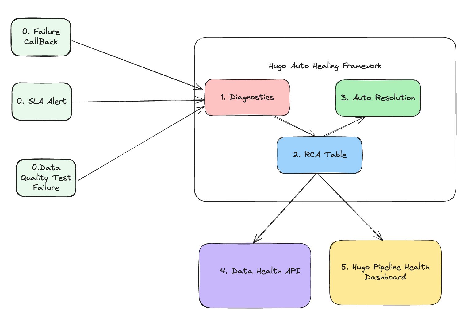
The architecture consists of five core modules, each with a specific function:
- Signal module: This module is responsible for collecting signals. It gathers three different types of signals that collectively define the health status of the data lake table. The signals include:
- Failure callback signal: This indicates whether the pipeline runs involving this data lake table are successful or not.
- SLA alert signal: This indicates whether the pipeline execution involving this data lake table meets the Service Level Agreement (SLA). For an hourly batch job, the expectation is to complete within one hour.
- Data quality test failure signal: This represents various types of completeness checks to ensure that data lake tables are consistent with the source tables based on their pipeline strategies.
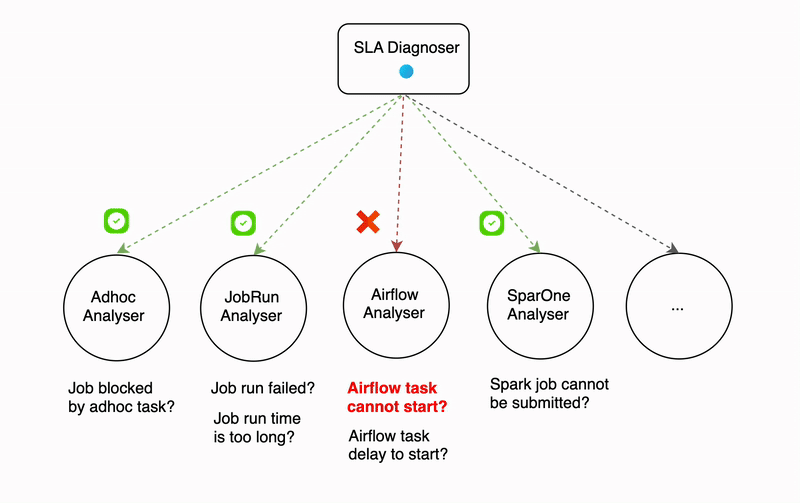
- Diagnosis module: This is the core module responsible for diagnosing the root cause of 3 types of failures collected in the Signal module. It determines:
- The root cause of the failure.
- The assignee responsible for fixing the error.
- The auto-resolution method to fix the issue.
- Manual resolution steps if the auto-resolution fails.
- RCA table: This module stores the following information:
- Signals
- Assignee information
- Diagnosis results
- Auto-resolution methods
- Manual resolution steps
- Auto-resolution module: This module executes the auto-resolution methods to resolve issues automatically.
- Data health API: This module provides API access to other platforms. External platforms or pipelines that rely on Hugo onboarded tables can subscribe to the health status and investigate the root cause when a table is deemed unhealthy.
- Hugo pipeline health dashboard: A centralised dashboard for Hugo users to visualise the health status of tables, auto resolution status, and manual fix button.
By leveraging these modules, the architecture ensures robust monitoring, diagnosis, and resolution of issues, leading to improved data health and operational efficiency.
Implementation
Signal module
There are two methods for generating these three signals. The failure signal is generated through an airflow callback, while the SLA miss and data completeness test signals are produced by Genchi. Genchi is a data quality observability platform at Grab that performs data quality checks and acts as a crucial enabler for the enforcement of data contracts.
Diagnosis module
As soon as an alert is created, the diagnosis begins. To avoid lengthy diagnosis times, Hugo has developed an innovative approach that eliminates the requirement for parsing extensive logs, such as Spark executor logs or Airflow logs. Instead, it gathers signals transmitted by the computation engine or Grab’s internal platforms.
The diagnosis process can be time-consuming, even with efforts to reduce the time it takes. For example, the SLA diagnoser uses multiple analysers that run sequentially, and some of these analysers (like the Airflow analyser) make API calls that can take a significant amount of time. The more analysers that are involved in the diagnosis process, the longer it can take.
Parallelism in diagnosis serves as a solution to lower the overall latency when there is a surge in error traffic. The degree of parallelism differs based on the type of signal. For example, the failure signal diagnosis can be executed in thousands of processes at once, while for SLA miss and data quality test failures signals, the parallelism is determined by the number of partitions in the Kafka topic since these signals are received from Kafka.
Auto-resolution module
Auto-resolution is a flexible framework that enables the implementation of custom handlers for various types of failures. One of the common handlers employs a retry mechanism with backoff for transient errors. For instance, if Hugo receives a failure callback indicating that the root cause is a database replica lag, it would wait for an hour before re-triggering the job. This auto-resolution process runs asynchronously with the diagnosis process.
Data health API
The data health information includes a unique identifier, current status, error details, and the time of the last health check, providing a comprehensive snapshot of the dataset’s health.
Hugo converts the detailed information available in its internal data health API to the data health API specification format to be consumed by Kinabalu, our internal system designed to automate and streamline incident management processes by integrating with multiple systems such as Slack, Jira, Splunk on-call, and Datadog.
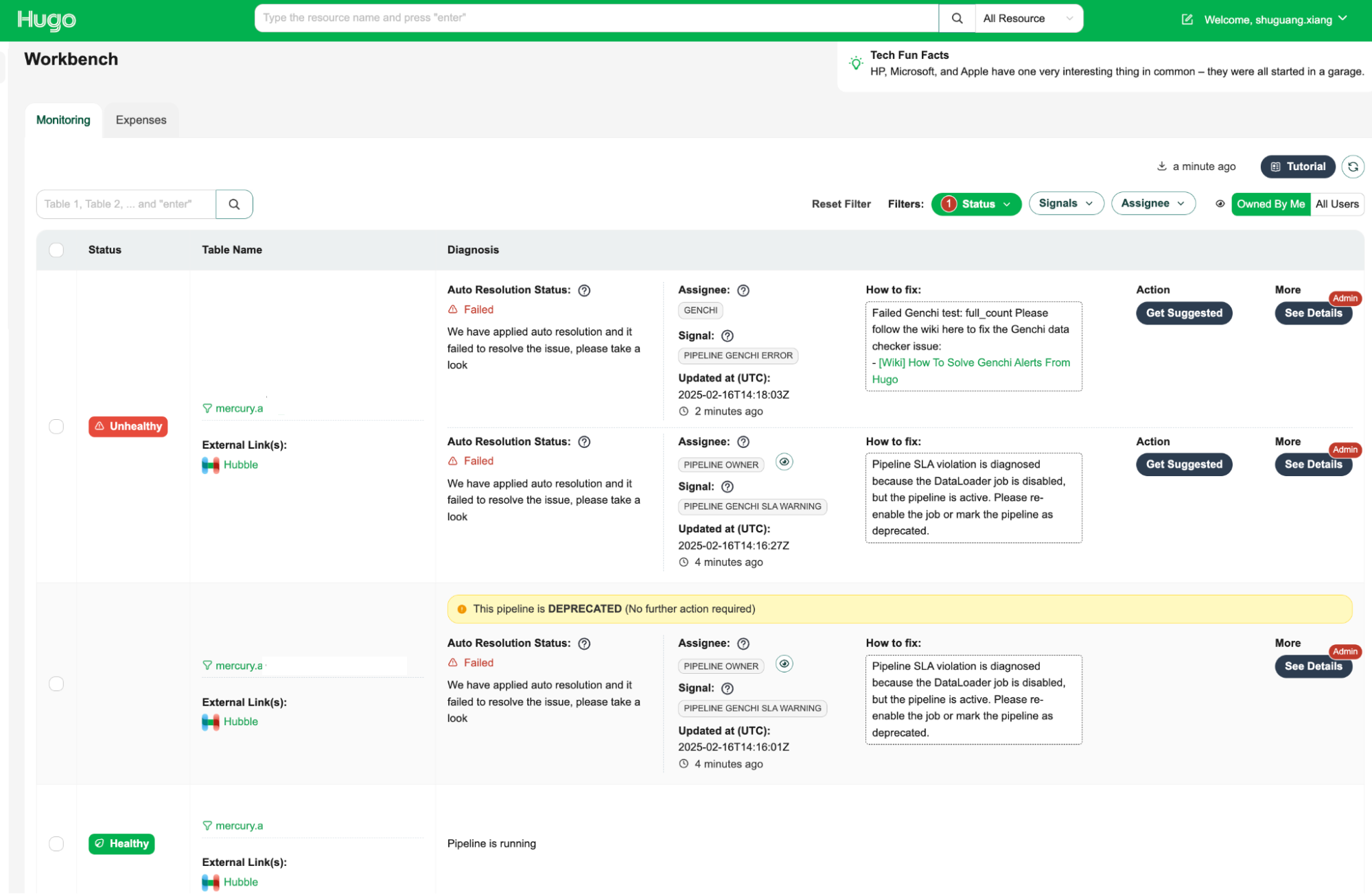
Hugo pipeline health dashboard
The Data Health Workbench is a centralised dashboard for Hugo users to visualise the health status of tables, auto-resolution status, and manual fix buttons. It provides a comprehensive view of data health and facilitates efficient issue resolution.
The key features are as follows:
- Health status visualisation: Displays the current health status of tables, making it easy to identify unhealthy tables.
- Assignee information: Indicates the assignee responsible for fixing the issue, ensuring clear accountability.
- How-to-fix guide: Provides step-by-step instructions on how to resolve the issue, empowering users to take immediate action.
- Action: Offers an action button to initiate the resolution process with a single click, streamlining issue resolution.
- Admin feature with detailed diagnosis information: Provides admins supplementary information, including the reasoning behind the root cause identification and assignee determination, which allows for a deeper understanding of the root cause of issues.
By leveraging the Data Health Workbench, Hugo users can efficiently monitor and manage data health, ensuring data integrity and operational efficiency.
Impact
The implementation of Hugo’s auto-healing and diagnosis features has resulted in significant improvements in stability and operational efficiency for our data pipelines. Here are some key outcomes:
- Enhanced data visibility: We’ve improved the visibility into the health of datasets, allowing for quick identification of issues and more informed decision-making.
- Timely resolution of data issues: With automated diagnostic and resolution processes, we ensure that data issues are addressed promptly, minimising data downtime and enhancing overall data availability.
- Reduced on-call workload: By automating many of the common failure resolutions, the workload on Hugo on-call teams has been significantly reduced. This allows teams to focus on more complex and impactful tasks.
- Scalable solution for managing complexity: The auto-resolution framework is well-equipped to handle the increasing complexity of data infrastructure, offering scalable solutions for transient errors through custom handlers and retry mechanisms.
- Improved data contract management: By providing detailed pipeline health information via the Data Health API, we enable precise and accurate DPIs, complete with root cause analysis and assignee information, enhancing the management and resolution of data contract breaches.
- Valuable reference for other platforms: The insights and methodologies developed through this initiative provide a valuable reference for other platform teams at Grab looking to implement similar automation and diagnostic capabilities.
- Support for Grab’s success: These enhancements support Grabbers by ensuring easy access to the datasets they need and contribute to the overall success of Grab through reliable data availability.
Next steps
Our next steps involve advancing auto-resolution strategies by focusing on complex solutions like pipeline runtime optimisation to boost efficiency and minimise processing delays. We will enrich the Data Health Workbench with detailed information, enabling users to visualise and understand pipeline health more effectively and make informed corrective actions. Additionally, we plan to broaden our diagnosis capabilities by integrating more infrastructure components, such as Flink health information, to ensure a comprehensive and holistic monitoring approach for all engines within Hugo.
Join us
Grab is a leading superapp in Southeast Asia, operating across the deliveries, mobility and digital financial services sectors. Serving over 800 cities in eight Southeast Asian countries, Grab enables millions of people everyday to order food or groceries, send packages, hail a ride or taxi, pay for online purchases or access services such as lending and insurance, all through a single app. Grab was founded in 2012 with the mission to drive Southeast Asia forward by creating economic empowerment for everyone. Grab strives to serve a triple bottom line – we aim to simultaneously deliver financial performance for our shareholders and have a positive social impact, which includes economic empowerment for millions of people in the region, while mitigating our environmental footprint.
Powered by technology and driven by heart, our mission is to drive Southeast Asia forward by creating economic empowerment for everyone. If this mission speaks to you, join our team today!