Southeast Asia (SEA) is a dynamic market, very different from other parts of the world. When travelling on the road, you may experience fast-changing road restrictions, new roads appearing overnight, and high traffic congestion. To address these challenges, GrabMaps has adapted to the SEA market by leveraging big data solutions. One of the solutions is the integration of hyperlocal data in GrabMaps.
Hyperlocal information is oriented around very small geographical communities and obtained from the local knowledge that our map team gathers. The map team is spread across SEA, enabling us to define clear specifications (e.g. legal speed limits), and validate that our solutions are viable.
Figure 1 – Map showing detections from images and probe data, and hyperlocal data.
Hyperlocal inputs make our mapping data even more robust, adding to the details collected from our image and probe detection pipelines. Figure 1 shows how data from our detection pipeline is overlaid with hyperlocal data, and then mapped across the SEA region. If you are curious and would like to check out the data yourself, you can download it here.
Processing hyperlocal data
Now let’s go through the process of detecting hyperlocal data.
Download data
GrabMaps is based on OpenStreetMap (OSM). The first step in the process is to download the .pbf file for Asia from geofabrick.de. This .pbf file contains all the data that is available on OSM, such as details of places, trees, and roads. Take for example a park, the .pbf file would contain data on the park name, wheelchair accessibility, and many more.
For this article, we will focus on hyperlocal data related to the road network. For each road, you can obtain data such as the type of road (residential or motorway), direction of traffic (one-way or more), and road name.
Convert data
To take advantage of big data computing, the next step in the process is to convert the .pbf file into Parquet format using a Parquetizer. This will convert the binary data in the .pbf file into a table format. Each road in SEA is now displayed as a row in a table as shown in Figure 2.
Figure 2 – Road data in Parquet format.
Identify hyperlocal data
After the data is prepared, GrabMaps then identifies and inputs all of our hyperlocal data, and delivers a consolidated view to our downstream services. Our hyperlocal data is obtained from various sources, either by looking at geometry, or other attributes in OSM such as the direction of travel and speed limit. We also apply customised rules defined by our local map team, all in a fully automated manner. This enhances the map together with data obtained from our rides and deliveries GPS pings and from KartaView, Grab’s product for imagery collection.
Figure 3 – Architecture diagram showing how hyperlocal data is integrated into GrabMaps.
Benefit of our hyperlocal GrabMaps
GrabNav, a turn-by-turn navigation tool available on the Grab driver app, is one of our products that benefits from having hyperlocal data. Here are some hyperlocal data that are made available through our approach:
Localisation of roads: The country, state/county, or city the road is in
Language spoken, driving side, and speed limit
Region-specific default speed regulations
Consistent name usage using language inference
Complex attributes like intersection links
To further explain the benefits of this hyperlocal feature, we will use intersection links as an example. In the next section, we will explain how intersection links data is used and how it impacts our driver-partners and passengers.
Identifying hyperlocal data – intersection links
An intersection link is when two or more roads meet. Figure 4 and 5 illustrates what an intersection link looks like in a GrabMaps mock and in OSM.
Figure 4 – Mock of an intersection link.
Figure 5 – Intersection link illustration from a real road network in OSM.
To locate intersection links in a road network, there are computations involved. We would first combine big data processing (which we do using Spark) with graphs. We use geohash as the unit of processing, and for each geohash, a bi-directional graph is created.
From such resulting graphs, we can determine intersection links if:
Road segments are parallel
The roads have the same name
The roads are one way roads
Angles and the shape of the road are in the intervals or requirements we seek
Each intersection link we identify is tagged in the map as intersection_links. Our downstream service teams can then identify them by searching for the tag.
Impact
The impact we create with our intersection link can be explained through the following example.
Figure 6 – Longer route, without GrabMaps intersection link feature. The arrow indicates where the route should have suggested a U-turn.
Figure 7 – Shorter route using GrabMaps by taking a closer link between two main roads.
Figure 6 and Figure 7 show two different routes for the same origin and destination. However, you can see that Figure 7 has a shorter route and this is made available by taking an intersection link early on in the route. The highlighted road segment in Figure 7 is an intersection link, tagged by the process we described earlier. The route is now much shorter making GrabNav more efficient in its route suggestion.
There are numerous factors that can impact a driver-partner’s trip, and intersection links are just one example. There are many more features that GrabMaps offers across Grab’s services that allow us to “outserve” our partners.
Conclusion
GrabMaps and GrabNav deliver enriched experiences to our driver-partners. By integrating certain hyperlocal data features, we are also able to provide more accurate pricing for both our driver-partners and passengers. In our mission towards sustainable growth, this is an area that we will keep on improving by leveraging scalable tech solutions.
Join us
Grab is the leading superapp platform in Southeast Asia, providing everyday services that matter to consumers. More than just a ride-hailing and food delivery app, Grab offers a wide range of on-demand services in the region, including mobility, food, package and grocery delivery services, mobile payments, and financial services across 428 cities in eight countries.
Powered by technology and driven by heart, our mission is to drive Southeast Asia forward by creating economic empowerment for everyone. If this mission speaks to you, join our team today!
We’re excited to announce a significant performance improvement coming to Workers KV, focused on dramatically improving cold read performance and reducing latency, even for long tail access patterns.
Developers using KV have seen great performance on hot reads, but ask why their 95th percentile latency — often on a key (or set of keys) that hadn’t been accessed recently or in that region — was higher than expected. We took this feedback to heart: we’ve been working feverishly on a new caching layer for KV behind the scenes, which enables customers to achieve much more frequent hot reads, reduced worst case latency times, better flexibility and control over cache TTLs, and much faster consistency over our previous iterations, and it’s now live for all KV users.
The best part? Developers using KV don’t need to change anything to benefit from this increased performance.
What is Workers KV?
Workers KV is a key value store designed for read heavy use-cases and applications powered by Cloudflare’s network. KV’s focus on read-heavy use-cases allows it to serve hot (cached) reads in milliseconds, which makes it ideal for storing per-application or customer configuration data, routing configuration, multivariate (A/B testing) configurations, and even small asset data that you need to serve quickly. Anything that you can serialize and need quickly you can store in KV, all the way up to 25 MiB worth of data per each individual key, with no cap on total data stored.
The problem
KV might be optimized for read-heavy workloads, but it’s critical that writes are globally available quickly enough that they’re useful for your application. Under typical conditions, the convergence delay for an eventually consistent system like KV is approximately one minute, globally: a write from one location should be able to be observed by all readers. Typical conditions are great, but typical unfortunately didn’t mean “always”. It could take significant time to restore global consistency where regions like North America and Europe are reading the same value. We needed to improve not just the average convergence, but the worst case as well.
Speaking of consistency, setting a long cache Time to Live (cacheTTL) for reads would result in a situation where you won’t notice a write for the entire cacheTTL duration, as the existing cached data had not timed out yet. This means you have to trade off read latency for infrequently accessed keys against noticing writes. Developers using KV have been consistent in their feedback: a higher cache TTL should improve performance, but not multiply the time it takes for KV to converge on a write to that key.
Lastly, our cold read times also left room for improvement. While cache hits are fast in KV, a cache miss would result in a request being routed all the way to our storage backends. While this is slow for everyone, it was particularly slow for folks in regions not immediately in the US or EU.This is poor performance that doesn’t represent what we can achieve with our global presence.
Our solution
A new horizontally scaled tiered cache
We’ve revamped Workers KV to be powered by a new tiered cache implementation. This implementation is written as a Worker service. We reuse the Dynamic Dispatch infrastructure developed for Workers for Platforms which lets us jump from our old KV worker into our new caching service within hundreds of microseconds. Importantly, this means we don’t impact cache hit performance to implement this new transparent caching layer. We leverage the same infrastructure powering Smart Placement to implement the tiering.
Before we re-designed KV, our topology looked like this:
All data centers in Cloudflare’s network can reach out to the origin in the event of a cache miss or to do a background refresh.
Cache TTL and efficiency
Our design goal was clear and ambitious: “can we relax honoring the cacheTTL constraint without violating it”? While this seems contradictory, the motivation is clear: we want to minimize the need to communicate with our storage backends while honoring the user-facing semantics of the cacheTTL setting, as it can have security implications if violated (e.g. if you use it to store and validate security tokens). Answering this design question also manages to simultaneously solve many of the problems outlined earlier.
Comparing existing solutions
First, let’s look at the design constraints for two eventually consistent storage systems at Cloudflare: Quicksilver and Tiered CDN.
Quicksilver gives us global consistency within seconds using a push architecture to replicate the data across all machines at Cloudflare. That architecture however doesn’t scale for Workers KV’s needs, which can have terabytes of data just within one namespace. This would be too much to replicate to every single data center.
By comparison, the tiered CDN cache is a pull mechanism where each hop pulls a more recent version of the asset into the local cache on access. That scales better because we only use storage for assets that are accessed, which works well with most use-cases where the vast majority of data is never retrieved. However, a pull based architecture is insufficient because it can only let us aggregate traffic across broader regions but we still can’t decouple how long we serve from the cache from the cacheTTL.
Push based architectures let us know when an asset is updated and enable scalable storage. By blending the properties of both systems, we can decouple how long we store the assets in cache from the cacheTTL. And that’s exactly what we did: KV now uses a hybrid push/pull caching layer where data centers closest to customers will pull from the regional data centers that are a little bit farther away. Writes will broadcast to all regional data centers that a key has been updated, so that the regional data center will remove that key from the local cache.
We can solve this problem by taking advantage of the fact that we semantically understand the write operations that are happening within Workers KV:
Workers KV doesn’t have one data center per region as might be typical for your zone in a Cloudflare CDN regional tiered cache topology. Instead, each key in a KV namespace is deterministically assigned a data center by performing a weighted rendezvous hash. The rendezvous hash ensures that load is distributed equally across the region and outages result in optimal shifts of traffic.
When the data center closest to a customer has a miss, it computes the regional data center affinity and provides that information to our Smart Placement infrastructure. When a regional tier misses, we repeat this process except using data centers in the KV origin region.
Finally, a miss at the upper tier exits to our storage nodes located in that origin region.
When we do a write, we only purge (invalidate) the key from the regional and upper tier data centers. This is a fixed number of data centers in our network regardless of how many data centers we add, which ensures that we aren’t reducing cache hit rates as our network continues to grow Compared with a global purge that delivers the event to every data center in our network, because we only need to deliver this purge to a random fixed set of data centers in our network, our aggregate write capacity for Workers KV automatically scales horizontally as we add more data centers.
All lower-tier data centers will reach out to a regional tier responsible for a given key in the event of a cache miss. If the regional tier doesn’t have the content, the regional tier will then ask an upper-tier out of region for the content. On a write for a given key, the responsible regional and upper tiers have that key deleted from cache.
Why do we call this a hybrid topology? The data centers closest to customers pull from the regional data centers as normal, but we automatically push invalidation events to the regional tier data centers on every write. That way, those customer data center pulls know to get an updated value when there is one. This means that while the cacheTTL parameter controls the caching behavior closest to the customer, it’s treated as a suggestion at best at the regional and upper tiers.
This way we’ve combined the push design principles behind Quicksilver, which delivers global consistency within seconds, with the pull-based design of our CDN tiered caching which can scale to handle “infinite” size workloads and prioritizes the assets that are most frequently accessed.
Visualizing it
It can be a bit hard to follow what’s happening in the new caching layer since there’s so many moving parts.
Here’s a video of a simplified version of how it works:
Small yellow balls represent KV read requests, larger green balls represent read responses. A larger purple ball represents a KV write request, while a read response ball represents a KV write response. Teal balls represent purge requests being broadcast. The “E” is a data center that doesn’t participate as a regional tier. The R represents the regional tier for key N while O is the upper tier for key N.
Decoupled cache TTL and consistency parameters
As a refresher, the objects written to KV can specify a cacheTTL: by default this is set to 1 minute, which is also the minimum acceptable value. This means that if an asset has been in the cache for longer than a minute, we bypass the cache and read instead from our durable storage nodes. In order to prevent eyeballs noticing origin fetches every minute, we implement stale while revalidate logic in our caching layer that automatically refreshes from the storage nodes in the background as requests come in.
Here’s an example from a Worker that’s constantly reading the same key
Notice the absence of any spikes indicating a cache miss? You’d expect to see them regularly every minute or so in the tens or even hundreds of milliseconds when the cacheTTL should expire. The reason this doesn’t happen is because as the expiry time is approaching, a background request to the storage nodes occurs and the cache is updated with an expiry time one more minute into the future; thus the asset in cache is never too stale and eyeball requests are always served from cache. Let’s take a look at requests to our storage layer before and after adding tiering:
Yellow is the estimated number of requests that would have occurred to origin without the new caching layer. Blue is the number of requests we’re making now.
The above chart is for a system with conservative parameters set. The upper tier doesn’t store the data for much longer than the cacheTTL currently and the upper tier will itself still do a background refresh probabilistically even though it doesn’t actually need to since we see all writes.
The new caching layer we’ve built inherits the old background refresh mechanism and expands on it. The first thing we did is decouple the background refresh period from the cacheTTL as a separate parameter (also defaulting to 1 minute). This means that even if you set a cacheTTL for 1 hour, KV will still check every minute from the regional tier to see if the value has been updated. If the data you’re storing within KV doesn’t have strict requirements on stale reads (think a key that’s accessed once every 10 minutes but needs to honor a write within 1 minute like security tokens), then you can increase the cacheTTL so that infrequently accessed keys stick around in the cache without changing the observed consistency.
Consistency improvements
Speaking of consistency, we’ve improved the worst case performance of that as well. Historically, we’ve had a background system that crawls all data in the storage nodes to figure out which region has the most up to date value and update accordingly. This gives us complete consistency coverage, but could take a significant amount of time to confirm. We would also periodically check both backends to see if network conditions had changed to pick the primary storage region to use for a given customer-close data center. Of course inconsistencies would be resolved then, but in practice this happens randomly, and at a low probability that won’t typically catch any meaningful values served inconsistently.
With the new caching layer all this changes. Since we’re now only reading keys on first access or after a write, we have enough storage capacity that we can check both backends on every read. When a customer requests data, we make a call to each origin data center, with the fastest response being returned immediately to reduce read latency. If the other data center has a newer value than what was returned first, we synchronize both data centers and notify our caching layer to purge that key from all regional data centers. If the other data center instead has an older value, we just synchronize the data centers without purging since we served the latest value. This means that even if our data centers are inconsistent, readers will notice new values much more quickly.
Latency improvements
Here’s the latency improvement at 10% rollout on a logarithmic x-axis:
Architecture that just gets better
This is just the start of what we can do. We now have a solid foundation for making further improvements, including making our best case reads even faster. We’ll be working on cutting out parts of our traditional stack that add unnecessary latency, and adding new high performance features that were too difficult to integrate otherwise. We can also explore features like setting the consistency TTL parameter for sub one minute consistency for additional cost. Similarly, we could create a best effort global purge feature if you want to choose to signal writes that way. Finally, we’re looking at exposing this new caching layer as a general Worker binding anyone can use within a Worker in front of their own service or to put in front of their Worker. If these sound like the killer features you need, please reach out to us if you’re interested in trying them out.
What next?
Developers don’t have to do anything to benefit from KV’s new performance improvements. We are currently in the process of rolling out our new architecture, and you don’t have to redeploy your Worker or change the way you use KV to benefit.
Workers KV is a natural fit for any application built on top of our Workers platform. We provide a native API that enables any Worker script to read, write, list, and manageyour Workers KV storage. You can also interact with Workers KV directly via our REST API from any client that can make a HTTP request, and the Cloudflare Dashboard provides an easy way to create, list, and delete keys to be used with the rest of your Workers setup.
Regardless of how you use Workers KV, it will be faster than ever before. We’re excited to see what you build with us, and you can dive into our documentation to start building with it.
Workers Analytics Engine is a new tool, announced earlier this year, that enables developers and product teams to build time series analytics about anything, with high dimensionality, high cardinality, and effortless scaling. We built Analytics Engine for teams to gain insights into their code running in Workers, provide analytics to end customers, or even build usage based billing.
In this blog post we’re going to tell you about how we use Analytics Engine to build Analytics Engine. We’ve instrumented our own Analytics Engine SQL API using Analytics Engine itself and use this data to find bugs and prioritize new product features. We hope this serves as inspiration for other teams who are looking for ways to instrument their own products and gather feedback.
Why do we need Analytics Engine?
Analytics Engine enables you to generate events (or “data points”) from Workers with just a few lines of code. Using the GraphQL or SQL API, you can query these events and create useful insights about the business or technology stack. For more about how to get started using Analytics Engine, check out our developer docs.
Since we released the Analytics Engine open beta in September, we’ve been adding new features at a rapid clip based on feedback from developers. However, we’ve had two big gaps in our visibility into the product.
First, our engineering team needs to answer classic observability questions, such as: how many requests are we getting, how many of those requests result in errors, what are the nature of these errors, etc. They need to be able to view both aggregated data (like average error rate, or p99 response time) and drill into individual events.
Second, because this is a newly launched product, we are looking for product insights. By instrumenting the SQL API, we can understand the queries our customers write, and the errors they see, which helps us prioritize missing features.
We realized that Analytics Engine would be an amazing tool for both answering our technical observability questions, and also gathering product insight. That’s because we can log an event for every query to our SQL API, and then query for both aggregated performance issues as well as individual errors and queries that our customers run.
In the next section, we’re going to walk you through how we use Analytics Engine to monitor that API.
Adding instrumentation to our SQL API
The Analytics Engine SQL API lets you query events data in the same way you would an ordinary database. For decades, SQL has been the most common language for querying data. We wanted to provide an interface that allows you to immediately start asking questions about your data without having to learn a new query language.
Our SQL API parses user SQL queries, transforms and validates them, and then executes them against backend database servers. We then write information about the query back into Analytics Engine so that we can run our own analytics. Writing data into Analytics Engine from a Cloudflare Worker is very simple and explained in our documentation. We instrument our SQL API in the same way our users do, and this code excerpt shows the data we write into Analytics Engine:
With that data now being stored in Analytics Engine, we can then pull out insights about every field we’re reporting.
Querying for insights
Having our analytics in an SQL database gives you the freedom to write any query you might want. Compared to using something like metrics which are often predefined and purpose specific, you can define any custom dataset desired, and interrogate your data to ask new questions with ease.
We need to support datasets comprising trillions of data points. In order to accomplish this, we have implemented a sampling method called Adaptive Bit Rate (ABR). With ABR, if you have large amounts of data, your queries may be returned sampled events in order to respond in reasonable time. If you have more typical amounts of data, Analytics Engine will query all your data. This allows you to run any query you like and still get responses in a short length of time. Right now, you have to account for sampling in how you make your queries, but we are exploring making it automatic.
Any data visualization tool can be used to visualize your analytics. At Cloudflare, we heavily use Grafana (and you can too!). This is particularly useful for observability use cases.
Observing query response times
One query we pay attention to gives us information about the performance of our backend database clusters:
As you can see, the 99% percentile (corresponding to the 1% most complex queries to execute) sometimes spikes up to about 300ms. But on average our backend responds to queries within 100ms.
This visualization is itself generated from an SQL query:
Customer insights from high-cardinality data
Another use of Analytics Engine is to draw insights out of customer behavior. Our SQL API is particularly well-suited for this, as you can take full advantage of the power of SQL. Thanks to our ABR technology, even expensive queries can be carried out against huge datasets.
We use this ability to help prioritize improvements to Analytics Engine. Our SQL API supports a fairly standard dialect of SQL but isn’t feature-complete yet. If a user tries to do something unsupported in an SQL query, they get back a structured error message. Those error messages are reported into Analytics Engine. We’re able to aggregate the kinds of errors that our customers encounter, which helps inform which features to prioritize next.
The SQL API returns errors in the format of type of error: more details, and so we can take the first portion before the colon to give us the type of error. We group by that, and get a count of how many times that error happened and how many users it affected:
To perform the above query using an ordinary metrics system, we would need to represent each error type with a different metric. Reporting that many metrics from each microservice creates scalability challenges. That problem doesn’t happen with Analytics Engine, because it’s designed to handle high-cardinality data.
Another big advantage of a high-cardinality store like Analytics Engine is that you can dig into specifics. If there’s a large spike in SQL errors, we may want to find which customers are having a problem in order to help them or identify what function they want to use. That’s easy to do with another SQL query:
Inside Cloudflare, we have historically relied on querying our backend database servers for this type of information. Analytics Engine’s SQL API now enables us to open up our technology to our customers, so they can easily gather insights about their services at any scale!
Conclusion and what’s next
The insights we gathered about usage of the SQL API are a super helpful input to our product prioritization decisions. We already added support for substring and position functions which were used in the visualizations above.
Looking at the top SQL errors, we see numerous errors related to selecting columns. These errors are mostly coming from some usability issues related to the Grafana plugin. Adding support for the DESCRIBE function should alleviate this because without this, the Grafana plugin doesn’t understand the table structure. This, as well as other improvements to our Grafana plugin, is on our roadmap.
We also can see that users are trying to query time ranges for older data that no longer exists. This suggests that our customers would appreciate having extended data retention. We’ve recently extended our retention from 31 to 92 days, and we will keep an eye on this to see if we should offer further extension.
We saw lots of errors related to common mistakes or misunderstandings of proper SQL syntax. This indicates that we could provide better examples or error explanations in our documentation to assist users with troubleshooting their queries.
Stay tuned into our developer docs to be informed as we continue to iterate and add more features!
You can start using Workers Analytics Engine Now! Analytics Engine is now in open beta with free 90-day retention. Start using it today or join our Discord community to talk with the team.
Cloudflare Radar was launched two years ago to give everyone access to the Internet trends, patterns and insights Cloudflare uses to help improve our service and protect our customers.
Until then, these types of insights were only available internally at Cloudflare. However, true to our mission of helping build a better Internet, we felt everyone should be able to look behind the curtain and see the inner workings of the Internet. It’s hard to improve or understand something when you don’t have clear visibility over how it’s working.
On Cloudflare Radar you can find timely graphs and visualizations on Internet traffic, security and attacks, protocol adoption and usage, and outages that might be affecting the Internet. All of these can be narrowed down by timeframe, country, and Autonomous System (AS). You can also find interactive deep dive reports on important subjects such as DDoS and the Meris Botnet. It’s also possible to search for any domain name to see details such as SSL usage and which countries their visitors are coming from.
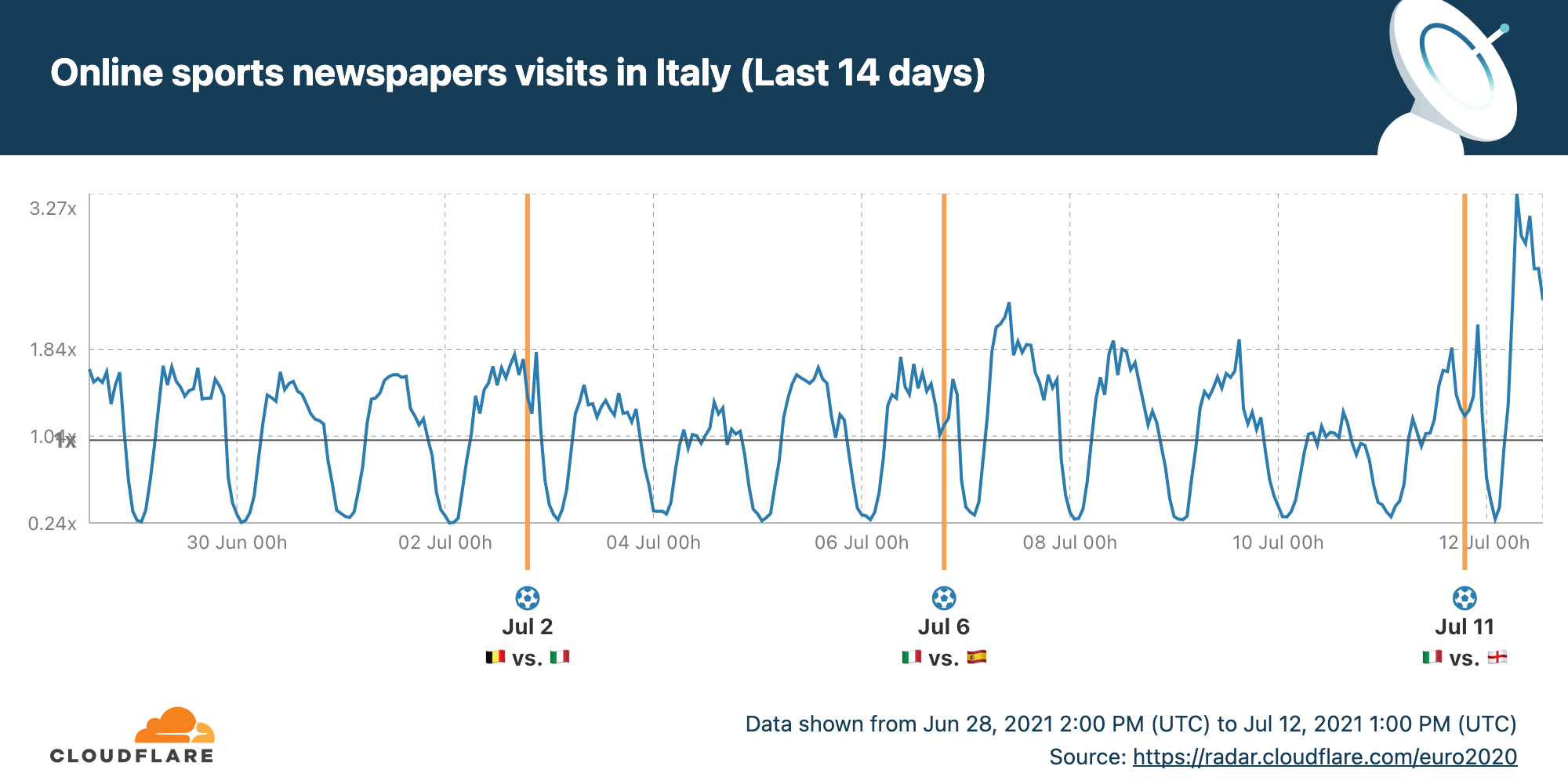
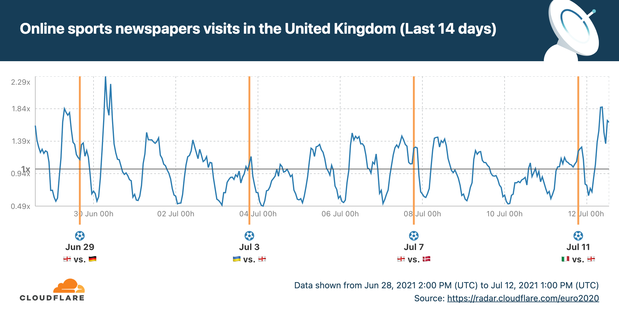
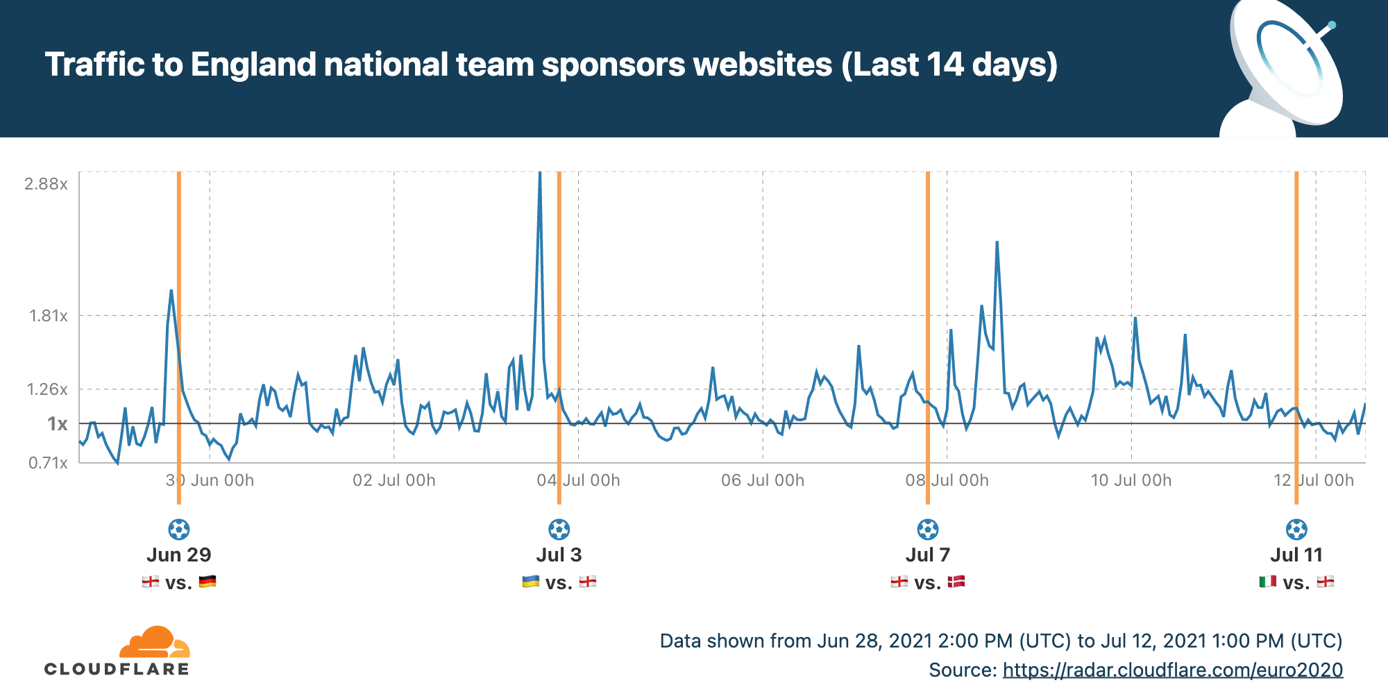
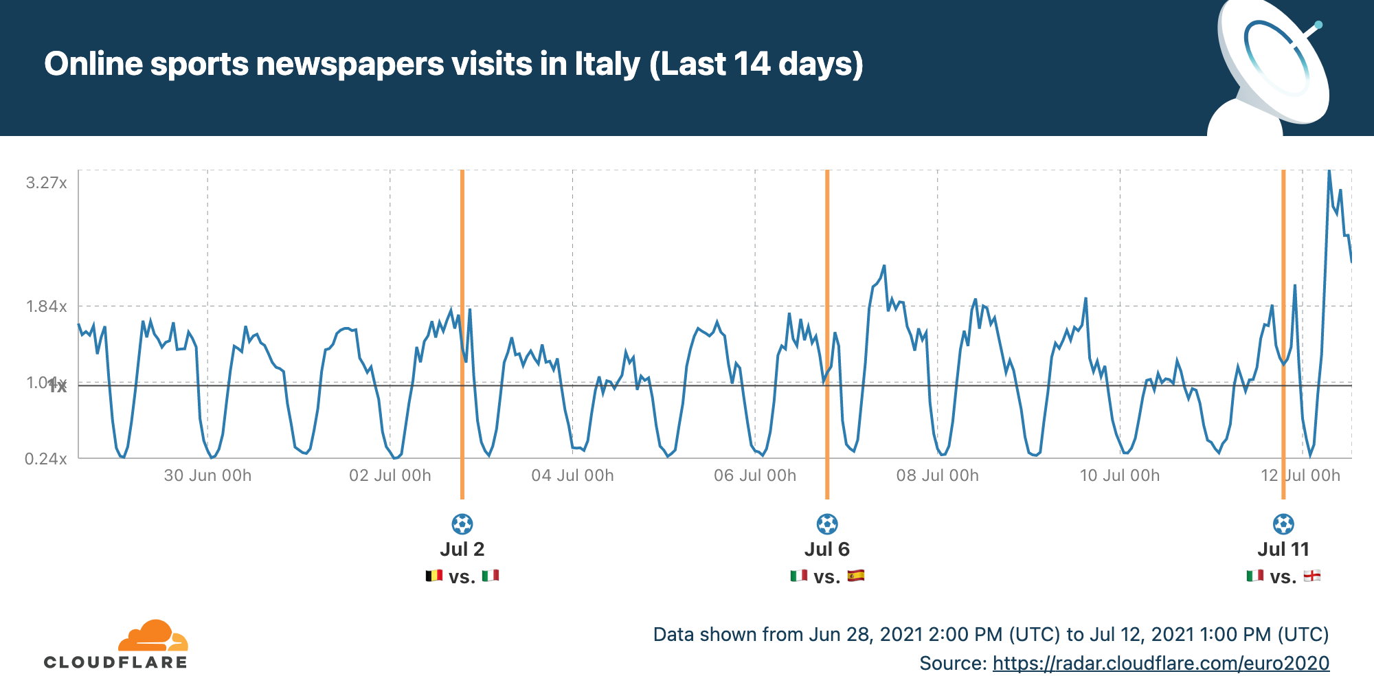
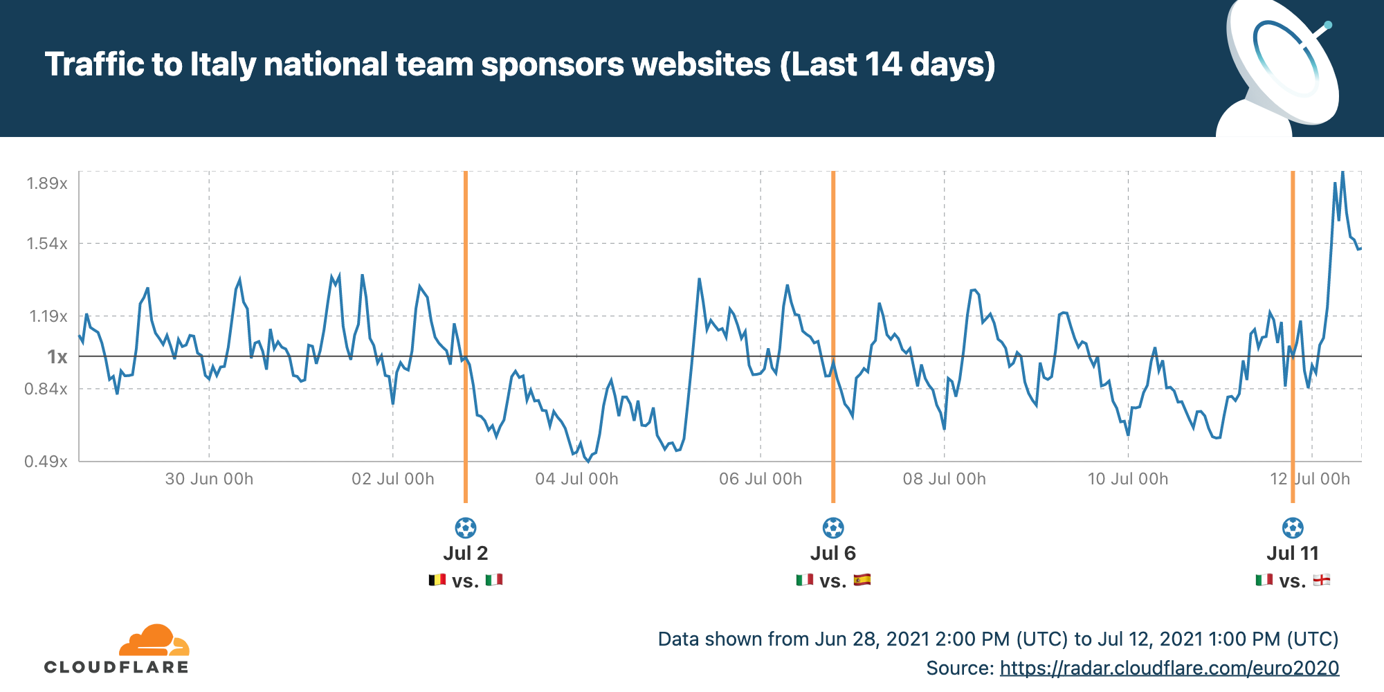
Since launch, Cloudflare Radar has been used by NGOs to confirm the Internet disruptions their observers see in the field, by journalists looking for Internet trends related to an event in a country of interest or at volume of cyberattacks as retaliation to political sanctions, by analysts looking at the prevalence of new protocols and technologies, and even by brand PR departments using Cloudflare Radar data to analyze the online impact of a major sports event.
Cloudflare Radar has clearly become an important tool for many and, most importantly, we find it has helped shed light on parts of the Internet that deserve more attention and investment.
Introducing Cloudflare Radar 2.0
What has made Cloudflare Radar so valuable is that the data and insights it contains are unique and trustworthy. Cloudflare Radar shows aggregate data from across the massive spectrum of Internet traffic we see every day, presenting you with datasets you won’t find elsewhere.
However, there were still gaps. Today, on the second anniversary of Cloudflare Radar, we are launching Cloudflare Radar 2.0 in beta. It will address three common pieces of feedback from users:
Ease of finding insights and data. The way information was structured on Cloudflare Radar made finding information daunting for some people. We are redesigning Cloudflare Radar so that it becomes a breeze.
Number of insights. We know many users have wanted to see insights about other important parts of the Internet, such as email. We have also completely redesigned the Cloudflare Radar backend so that we can quickly add new insights over the coming months (including insights into email).
Sharing insights.The options for sharing Cloudflare Radar insights were limited. We will now provide you the options you want, including downloadable and embeddable graphs, sharing to social media platforms, and an API.
Finding insights and data
On a first visit to the redesigned Cloudflare Radar homepage one will notice:
Prominent and intuitive filtering capabilities on the top bar. A global search bar is also coming soon.
Content navigation on the sidebar.
Content cards showing glanceable and timely information.
The content you find on the homepage are what we call “quick bytes”. Those link you to more in-depth content for that specific topic, which can also be found through the sidebar navigation.
At the top of the page you can search for a country, autonomous system number (ASN), domain, or report to navigate to a home page for that specific content. For example, the domain page for google.com:
The navigation sidebar allows you to find more detailed insights and data related to Traffic, Security & Attacks, Adoption & Usage, and Domains. (We will be adding additional topic areas in the future.) It also gives you quick access to the Cloudflare Radar Outage Center, a tool for tracking Internet disruptions around the world and to which we are dedicating a separate blog post, and to Radar Reports, which are interactive deep dive reports on important subjects such as DDoS and the Meris Botnet.
Within these topic pages (such as the one for Adoption & Usage shown above), you will find the quick bytes for the corresponding topic at the top, and quick bytes for related topics on the right. The quick bytes on the right allow you to quickly glance at and navigate to related sections.
In the middle of the page are the more detailed charts for the topic you’re exploring.
Sharing insights
Cloudflare Radar’s reason to exist is to make Internet insights available to everyone, but historically we haven’t been as flexible as our users would want. People could download a snapshot of the graph, but not much more.
With Cloudflare Radar 2.0 we will be introducing three major new ways of using Radar insights and data:
Social share. Cloudflare Radar 2.0 charts have a more modern and clean look and feel, and soon you’ll be able to share them directly on the social media platform of your choice. No more dealing with low quality screenshots.
Embeddable charts. The beautiful charts will also be able to be embedded directly into your webpage or blog – it will work just like a widget, always showing up-to-date information.
API. If you like the data on Cloudflare Radar but want to manipulate it further for analysis, visualization, or for posting your own charts, you’ll have the Cloudflare Radar API available to you starting today.
Note: The API is available today. To use the Cloudflare API you need an API token or key (more details here). Embedding charts and sharing directly to social are new features to be released later this year.
Technology changes
Cloudflare Radar 2.0 was built on a new technology stack; we will write a blog post about why and how we did it soon. A lot changed: we now have proper GraphQL data endpoints and a public API, the website runs on top of Cloudflare Pages and Workers, and we’re finally doing server-side rendering using Remix. We adopted SVG whenever possible, built our reusable data visualization components system, and are using Cosmos for visual TDD. These foundational changes will provide a better UX/UI to our users and give us speed when iterating and improving Cloudflare Radar in the future.
We hope you find this update valuable, and recommend you keep an eye on radar.cloudflare.com to see the new insights and topics we’ll be adding regularly. If you have any feedback, please send it to us through the Cloudflare Community.
We’re excited to announce the availability of Network Analytics Logs. Magic Transit, Magic Firewall, Magic WAN, and Spectrum customers on the Enterprise plan can feed packet samples directly into storage services, network monitoring tools such as Kentik, or their Security Information Event Management (SIEM) systems such as Splunk to gain near real-time visibility into network traffic and DDoS attacks.
What’s included in the logs
By creating a Network Analytics Logs job, Cloudflare will continuously push logs of packet samples directly to the HTTP endpoint of your choice, including Websockets. The logs arrive in JSON format which makes them easy to parse, transform, and aggregate. The logs include packet samples of traffic dropped and passed by the following systems:
Network-layer DDoS Protection Ruleset
Advanced TCP Protection
Magic Firewall
Note that not all mitigation systems are applicable to all Cloudflare services. Below is a table describing which mitigation service is applicable to which Cloudflare service:
Mitigation System
Cloudflare Service
Magic Transit
Magic WAN
Spectrum
Network-layer DDoS Protection Ruleset
✅
❌
✅
Advanced TCP Protection
✅
❌
❌
Magic Firewall
✅
✅
❌
Packets are processed by the mitigation systems in the order outlined above. Therefore, a packet that passed all three systems may produce three packet samples, one from each system. This can be very insightful when troubleshooting and wanting to understand where in the stack a packet was dropped. To avoid overcounting the total passed traffic, Magic Transit users should only take into consideration the passed packets from the last mitigation system, Magic Firewall.
In this walkthrough, we will demonstrate how to feed the Network Analytics Logs into Splunk via Postman. At this time, it is only possible to set up Network Analytics Logs via API. Setting up the logs requires three main steps:
Create a Cloudflare API token.
Create a Splunk Cloud HTTP Event Collector (HEC) token.
Create and enable a Cloudflare Logpush job.
Let’s get started!
1) Create a Cloudflare API token
Log in to your Cloudflare account and navigate to My Profile.
On the left-hand side, in the collapsing navigation menu, click API Tokens.
Click Create Token and then, under Custom token, click Get started.
Give your custom token a name, and select an Account scoped permission to edit Logs. You can also scope it to a specific/subset/all of your accounts.
At the bottom, click Continue to summary, and then Create Token.
Copy and save your token. You can also test your token with the provided snippet in Terminal.
When you’re using an API token, you don’t need to provide your email address as part of the API credentials.
Creating and enabling a job is very straightforward. It requires only one API call to Cloudflare to create and enable a job.
To send the API calls I used Postman, which is a user-friendly API client that was recommended to me by a colleague. It allows you to save and customize API calls. You can also use Terminal/CMD or any other API client/script of your choice.
One thing to notice is Network Analytics Logs are account-scoped. The API endpoint is therefore a tad different from what you would normally use for zone-scoped datasets such as HTTP request logs and DNS logs.
This is the endpoint for creating an account-scoped Logpush job:
Your account identifier number is a unique identifier of your account. It is a string of 32 numbers and characters. If you’re not sure what your account identifier is, log in to Cloudflare, select the appropriate account, and copy the string at the end of the URL.
https://dash.cloudflare.com/{account-id}
Then, set up a new request in Postman (or any other API client/CLI tool).
To successfully create a Logpush job, you’ll need the HTTP method, URL, Authorization token, and request body (data). The request body must include a destination configuration (destination_conf), the specified dataset (network_analytics_logs, in our case), and the token (your Splunk token).
Depending on the amount of logs that you read and write, the cost of third party cloud storage can skyrocket — forcing you to decide between managing a tight budget and being able to properly investigate networking and security issues. However, we believe that you shouldn’t have to make those trade-offs. With R2’s low costs, we’re making this decision easier for our customers. Instead of feeding logs to a third party, you can reap the cost benefits of storing them in R2.
To learn more about the R2 features and pricing, check out the full blog post. To enable R2, contact your account team.
Cloudflare logs for maximum visibility
Cloudflare Enterprise customers have access to detailed logs of the metadata generated by our products. These logs are helpful for troubleshooting, identifying network and configuration adjustments, and generating reports, especially when combined with logs from other sources, such as your servers, firewalls, routers, and other appliances.
Not using Cloudflare yet? Start now with our Free and Pro plans to protect your websites against DDoS attacks, or contact us for comprehensive DDoS protection and firewall-as-a-service for your entire network.
Data localisation has gotten a lot of attention in recent years because a number of countries see it as a way of controlling or protecting their citizens’ data. Countries such as Australia, China, India, Brazil, and South Korea have or are currently considering regulations that assert legal sovereignty over their citizens’ personal data in some fashion — health care data must be stored locally; public institutions may only contract with local service providers, etc.
In the EU, the recent “Schrems II” decision resulted in additional requirements for companies that transfer personal data outside the EU. And a number of highly regulated industries require that specific types of personal data stay within the EU’s borders.
Cloudflare is committed to helping our customers keep personal data in the EU. Last year, we introduced the Data Localisation Suite, which gives customers control over where their data is inspected and stored.
Today, we’re excited to introduce the Customer Metadata Boundary, which expands the Data Localisation Suite to ensure that a customer’s end user traffic metadata stays in the EU.
Metadata: a primer
“Metadata” can be a scary term, but it’s a simple concept — it just means “data about data.” In other words, it’s a description of activity that happened on our network. Every service on the Internet collects metadata in some form, and it’s vital to user safety and network availability.
At Cloudflare, we collect metadata about the usage of our products for several purposes:
Serving analytics via our dashboards and APIs
Sharing logs with customers
Stopping security threats such as bot or DDoS attacks
Improving the performance of our network
Maintaining the reliability and resiliency of our network
What does that collection look like in practice at Cloudflare? Our network consists of dozens of services: our Firewall, Cache, DNS Resolver, DDoS protection systems, Workers runtime, and more. Each service emits structured log messages, which contain fields like timestamps, URLs, usage of Cloudflare features, and the identifier of the customer’s account and zone.
These messages do not contain the contents of customer traffic, and so they do not contain things like usernames, passwords, personal information, and other private details of customers’ end users. However, these logs may contain end-user IP addresses, which is considered personal data in the EU.
Data Localisation in the EU
The EU’s General Data Protection Regulation, or GDPR, is one of the world’s most comprehensive (and well known) data privacy laws. The GDPR does not, however, insist that personal data must stay in Europe. Instead, it provides a number of legal mechanisms to ensure that GDPR-level protections are available for EU personal data if it is transferred outside the EU to a third country like the United States. Data transfers from the EU to the US were, until recently, permitted under an agreement called the EU-U.S. Privacy Shield Framework.
Shortly after the GDPR went into effect, a privacy activist named Max Schrems filed suit against Facebook for their data collection practices. In July 2020, the Court of Justice of the EU issued the “Schrems II” ruling — which, among other things, invalidated the Privacy Shield framework. However, the court upheld other valid transfer mechanisms that ensure EU personal data won’t be accessed by U.S. government authorities in a way that violates the GDPR.
Since the Schrems II decision, many customers have asked us how we’re protecting EU citizens’ data. Fortunately, Cloudflare has had data protection safeguards in place since well before the Schrems II case, such as our industry-leading commitments on government data requests. In response to Schrems II in particular, we updated our customer Data Processing Addendum (DPA). We incorporated the latest Standard Contractual Clauses, which are legal agreements approved by the EU Commission that enable data transfer. We also added additional safeguards as outlined in the EDPB’s June 2021 Recommendations on Supplementary Measures. Finally, Cloudflare’s services are certified under the ISO 27701 standard, which maps to the GDPR’s requirements.
In light of these measures, we believe that our EU customers can use Cloudflare’s services in a manner consistent with GDPR and the Schrems II decision. Still, we recognize that many of our customers want their EU personal data to stay in the EU. For example, some of our customers in industries like healthcare, law, and finance may have additional requirements. For that reason, we have developed an optional suite of services to address those requirements. We call this our Data Localisation Suite.
How the Data Localisation Suite helps today
Data Localisation is challenging for customers because of the volume and variety of data they handle. When it comes to their Cloudflare traffic, we’ve found that customers are primarily concerned about three areas:
How do I ensure my encryption keys stay in the EU?
How can I ensure that services like caching and WAF only run in the EU?
How can ensure that metadata is never transferred outside the EU?
To address the first concern, Cloudflare has long offered Keyless SSL and Geo Key Manager, which ensure that private SSL/TLS key material never leaves the EU. Keyless SSL ensures that Cloudflare never has possession of the private key material at all; Geo Key Manager uses Keyless SSL under the hood to ensure the keys never leave the specified region.
Last year we addressed the second concern with Regional Services, which ensures that Cloudflare will only be able to decrypt and inspect the content of HTTP traffic inside the EU. In other words, SSL connections will only be terminated in Europe, and all of our layer 7 security and performance services will only run in our EU data centers.
Today, we’re enabling customers to address the third and final concern, and keep metadata local as well.
How the Metadata Boundary Works
The Customer Metadata Boundary ensures, simply, that end user traffic metadata that can identify a customer stays in the EU. This includes all the logs and analytics that a customer sees.
How are we able to do this? All the metadata that can identify a customer flows through a single service at our edge, before being forwarded to one of our core data centers.
When the Metadata Boundary is enabled for a customer, our edge ensures that any log message that identifies that customer (that is, contains that customer’s Account ID) is not sent outside the EU. It will only be sent to our core data center in the EU, and not our core data center in the US.
What’s next
Today our Data Localisation Suite is focused on helping our customers in the EU localise data for their inbound HTTP traffic. This includes our Cache, Firewall, DDoS protection, and Bot Management products.
We’ve heard from customers that they want data localisation for more products and more regions. This means making all of our Data Localisation Products, including Geo Key Manager and Regional Services, work globally. We’re also working on expanding the Metadata Boundary to include our Zero Trust products like Cloudflare for Teams. Stay tuned!
Data Engineers of Netflix — Interview with Pallavi Phadnis
This post is part of our “Data Engineers of Netflix” series, where our very own data engineers talk about their journeys to Data Engineering @ Netflix.
Pallavi Phadnis is a Senior Software Engineer at Netflix.
Pallavi Phadnis is a Senior Software Engineer on the Product Data Science and Engineering team. In this post, Pallavi talks about her journey to Netflix and the challenges that keep the work interesting.
Pallavi received her master’s degree from Carnegie Mellon. Before joining Netflix, she worked in the advertising and e-commerce industries as a backend software engineer. In her free time, she enjoys watching Netflix and traveling.
Her favorite shows: Stranger Things, Gilmore Girls, and Breaking Bad.
Pallavi, what’s your journey to data engineering at Netflix?
Netflix’s unique work culture and petabyte-scale data problems are what drew me to Netflix.
During earlier years of my career, I primarily worked as a backend software engineer, designing and building the backend systems that enable big data analytics. I developed many batch and real-time data pipelines using open source technologies for AOL Advertising and eBay. I also built online serving systems and microservices powering Walmart’s e-commerce.
Those years of experience solving technical problems for various businesses have taught me that data has the power to maximize the potential of any product.
Before I joined Netflix, I was always fascinated by my experience as a Netflix member which left a great impression of Netflix engineering teams on me. When I read Netflix’s culture memo for the first time, I was impressed by how candid, direct and transparent the work culture sounded. These cultural points resonated with me most: freedom and responsibility, high bar for performance, and no hiring of brilliant jerks.
Over the years, I followed the big data open-source community and Netflix tech blogs closely, and learned a lot about Netflix’s innovative engineering solutions and active contributions to the open-source ecosystem. In 2017, I attended the Women in Big Data conference at Netflix and met with several amazing women in data engineering, including our VP. At this conference, I also got to know my current team: Consolidated Logging (CL).
CL provides an end-to-end solution for logging, processing, and analyzing user interactions on Netflix apps from all devices. It is critical for fast-paced product innovation at Netflix since CL provides foundational data for personalization, A/B experimentation, and performance analytics. Moreover, its petabyte scale also brings unique engineering challenges. The scope of work, business impact, and engineering challenges of CL were very exciting to me. Plus, the roles on the CL team require a blend of data engineering, software engineering, and distributed systems skills, which align really well with my interests and expertise.
What is your favorite project?
The project I am most proud of is building the Consolidated Logging V2 platform which processes and enriches data at a massive scale (5 million+ events per sec at peak) in real-time. I re-architected our legacy data pipelines and built a new platform on top of Apache Flink and Iceberg. The scale brought some interesting learnings and involved working closely with the Apache Flink and Kafka community to fix core issues. Thanks to the migration to V2, we were able to improve data availability and usability for our consumers significantly. The efficiency achieved in processing and storage layers brought us big savings on computing and storage costs. You can learn more about it from my talk at the Flink forward conference. Over the last couple of years, we have been continuously enhancing the V2 platform to support more logging use cases beyond Netflix streaming apps and provide further analytics capabilities. For instance, I am recently working on a project to build a common analytics solution for 100s of Netflix studio and internal apps.
How’s data engineering similar and different from software engineering?
The data engineering role at Netflix is similar to the software engineering role in many aspects. Both roles involve designing and developing large-scale solutions using various open-source technologies. In addition to the business logic, they need a good understanding of the framework internals and infrastructure in order to ensure production stability, for example, maintaining SLA to minimize the impact on the upstream and downstream applications. At Netflix, it is fairly common for data engineers and software engineers to collaborate on the same projects.
In addition, data engineers are responsible for designing data logging specifications and optimized data models to ensure that the desired business questions can be answered. Therefore, they have to understand both the product and the business use cases of the data in depth.
In other words, data engineers bridge the gap between data producers (such as client UI teams) and data consumers (such as data analysts and data scientists.)
Learning more
Interested in learning more about data roles at Netflix? You’re in the right place! Keep an eye out for our open roles in Data Science and Engineering by visiting our jobs site here. Our culture is key to our impact and growth: read about it here. To learn more about our Data Engineers, check out our chats with Dhevi Rajendran, Samuel Setegne, and Kevin Wylie.
Modern applications commonly utilise various database engines, with each serving a specific need. At Grab Deliveries, MySQL database (DB) is utilised to store canonical forms of data, and ElasticSearch (ES) to provide advanced search capabilities. MySQL serves as the primary data storage for raw data, and ES as the derived storage.
Search data flow
Efforts have been made to synchronise data between MySQL and ES. In this post, a series of techniques will be introduced on how to optimise incremental search data indexing.
Background
The synchronisation of data from the primary data storage to the derived data storage is handled by Food-Puxian, a Data Synchronisation Platform (DSP). In a search service context, it is the synchronisation of data between MySQL and ES.
The data synchronisation process is triggered on every real-time data update to MySQL, which will streamline the updated data to Kafka. DSP consumes the list of Kafka streams and incrementally updates the respective search indexes in ES. This process is also known as Incremental Sync.
Kafka to DSP
DSP uses Kafka streams to implement Incremental Sync. A stream represents an unbounded, continuously updating data set. A stream is ordered, replayable and is a fault-tolerant sequence of immutable.
Data synchronisation process using Kafka
The above diagram depicts the process of data synchronisation using Kafka. The Data Producer creates a Kafka stream for every operation done on MySQL and sends it to Kafka in real-time. DSP creates a stream consumer for each Kafka stream and the consumer reads data updates from respective Kafka streams and synchronises them to ES.
MySQL to ES
Indexes in ES correspond to tables in MySQL. MySQL data is stored in tables, while ES data is stored in indexes. Multiple MySQL tables are joined to form an ES index. The below snippet shows the Entity-Relationship mapping in MySQL and ES. Entity A has a one-to-many relationship with entity B. Entity A has multiple associated tables in MySQL, table A1 and A2, and they are joined into a single ES index A.
ER mapping in MySQL and ES
Sometimes a search index contains both entity A and entity B. In a keyword search query on this index, e.g. “Burger”, objects from both entity A and entity B whose name contains “Burger” are returned in the search response.
Original Incremental Sync
Original Kafka streams
The Data Producers create a Kafka stream for every MySQL table in the ER diagram above. Every time there is an insert/update/delete operation on the MySQL tables, a copy of the data after the operation executes is sent to its Kafka stream. DSP creates different stream consumers for every Kafka stream since their data structures are different.
Stream Consumer infrastructure
Stream Consumer consists of 3 components.
Event Dispatcher: Listens and fetches events from the Kafka stream, pushes them to the Event Buffer and starts a goroutine to run Event Handler for every event whose ID does not exist in the Event Buffer
Event Buffer: Caches events in memory by the primary key (aID, bID, etc). An event is cached in the Buffer until it is picked by a goroutine or replaced when a new event with the same primary key is pushed into the Buffer.
Event Handler: Reads an event from the Event Buffer and the goroutine started by the Event Dispatcher handles it.
Stream consumer infrastructure
Event Buffer procedure
Event Buffer consists of many sub buffers, each with a unique ID which is the primary key of the event cached in it. The maximum size of a sub buffer is 1. This allows Event Buffer to deduplicate events having the same ID in the buffer.
The below diagram shows the procedure of pushing an event to Event Buffer. When a new event is pushed to the buffer, the old event sharing the same ID will be replaced. The replaced event is therefore not handled.
Pushing an event to the Event Buffer
Event Handler procedure
The below flowchart shows the procedures executed by the Event Handler. It consists of the common handler flow (in white), and additional procedures for object B events (in green). After creating a new ES document by data loaded from the database, it will get the original document from ES to compare if any field is changed and decide whether it is necessary to send the new document to ES.
When object B event is being handled, on top of the common handler flow, it also cascades the update to the related object A in the ES index. We name this kind of operation Cascade Update.
Procedures executed by the Event Handler
Issues in the original infrastructure
Data in an ES index can come from multiple MySQL tables as shown below.
Data in an ES index
The original infrastructure came with a few issues.
Heavy DB load: Consumers read from Kafka streams, treat stream events as notifications then use IDs to load data from the DB to create a new ES document. Data in the stream events are not well utilised. Loading data from the DB every time to create a new ES document results in heavy traffic to the DB. The DB becomes a bottleneck.
Data loss: Producers send data copies to Kafka in application code. Data changes made via MySQL command-line tool (CLT) or other DB management tools are lost.
Tight coupling with MySQL table structure: If producers add a new column to an existing table in MySQL and this column needs to be synchronised to ES, DSP is not able to capture the data changes of this column until the producers make the code change and add the column to the related Kafka Stream.
Redundant ES updates: ES data is a subset of MySQL data. Producers publish data to Kafka streams even if changes are made on fields that are not relevant to ES. These stream events that are irrelevant to ES would still be picked up.
Duplicate cascade updates: Consider a case where the search index contains both object A and object B. A large number of updates to object B are created within a short span of time. All the updates will be cascaded to the index containing both objects A and B. This will bring heavy traffic to the DB.
Optimised Incremental Sync
MySQL Binlog
MySQL binary log (Binlog) is a set of log files that contain information about data modifications made to a MySQL server instance. It contains all statements that update data. There are two types of binary logging:
Statement-based logging: Events contain SQL statements that produce data changes (inserts, updates, deletes).
Row-based logging: Events describe changes to individual rows.
The Grab Caspian team (Data Tech) has built a Change Data Capture (CDC) system based on MySQL row-based Binlog. It captures all the data modifications made to MySQL tables.
Current Kafka streams
The Binlog stream event definition is a common data structure with three main fields: Operation, PayloadBefore and PayloadAfter. The Operation enums are Create, Delete, and Update. Payloads are the data in JSON string format. All Binlog streams follow the same stream event definition. Leveraging PayloadBefore and PayloadAfter in the Binlog event, optimisations of incremental sync on DSP becomes possible.
Binlog stream event main fields
Stream Consumer optimisations
Event Handler optimisations
Optimisation 1
Remember that there was a redundant ES updates issue mentioned above where the ES data is a subset of the MySQL data. The first optimisation is to filter out irrelevant stream events by checking if the fields that are different between PayloadBefore and PayloadAfter are in the ES data subset.
Since the payloads in the Binlog event are JSON strings, a data structure only with fields that are present in ES data is defined to parse PayloadBefore and PayloadAfter. By comparing the parsed payloads, it is easy to know whether the change is relevant to ES.
The below diagram shows the optimised Event Handler flows. As shown in the blue flow, when an event is handled, PayloadBefore and PayloadAfter are compared first. An event will be processed only if there is a difference between PayloadBefore and PayloadAfter. Since the irrelevant events are filtered, it is unnecessary to get the original document from ES.
Event Handler optimisation 1
Achievements
No data loss: changes made via MySQL CLT or other DB manage tools can be captured.
No dependency on MySQL table definition: All the data is in JSON string format.
No redundant ES updates and DB reads.
ES reads traffic reduced by 90%: Not a need to get the original document from ES to compare with the newly created document anymore.
55% irrelevant stream events filtered out
DB load reduced by 55%
ES event updates for optimisation 1
Optimisation 2
The PayloadAfter in the event provides updated data. This makes us think about whether a completely new ES document is needed each time, with its data read from several MySQL tables. The second optimisation is to change to a partial update using data differences from the Binlog event.
The below diagram shows the Event Handler procedure flow with a partial update. As shown in the red flow, instead of creating a new ES document for each event, a check on whether the document exists will be performed first. If the document exists, which happens for the majority of the time, the data is changed in this event, provided the comparison between PayloadBefore and PayloadAfter is updated to the existing ES document.
Event Handler optimisation 2
Achievements
Change most ES relevant events to partial update: Use data in stream events to update ES.
ES load reduced: Only fields that have been changed will be sent to ES.
DB load reduced: DB load reduced by 80% based on Optimisation 1.
ES event updates for optimisation 2
Event Buffer optimisation
Instead of replacing the old event, we merge the new event with the old event when the new event is pushed to the Event Buffer.
The size of each sub buffer in Event Buffer is 1. In this optimisation, the stream event is not treated as a notification anymore. We use the Payloads in the event to perform Partial Updates. The old procedure of replacing old events is no longer suitable for the Binlog stream.
When the Event Dispatcher pushes a new event to a non-empty sub buffer in the Event Buffer, it will merge event A in the sub buffer and the new event B into a new Binlog event C, whose PayloadBefore is from Event A and PayloadAfter is from Event B.
Merge operation for Event Buffer optimisation
Cascade Update optimisation
Optimisation
Use a new stream to handle cascade update events.
When the producer sends data to the Kafka stream, data sharing the same ID will be stored at the same partition. Every DSP service instance has only one stream consumer. When Kafka streams are consumed by consumers, one partition will be consumed by only one consumer. So the Cascade Update events sharing the same ID will be consumed by one stream consumer on the same EC2 instance. With this special mechanism, the in-memory Event Buffer is able to deduplicate most of the Cascade Update events sharing the same ID.
The flowchart below shows the optimised Event Handler procedure. Highlighted in green is the original flow while purple highlights the current flow with Cascade Update events.
When handling an object B event, instead of cascading update the related object A directly, the Event Handler will send a Cascade Update event to the new stream. The consumer of the new stream will handle the Cascade Update event and synchronise the data of object A to the ES.
Event Handler with Cascade Update events
Achievements
Cascade Update events deduplicated by 80%
DB load introduced by cascade update reduced
Cascade Update events
Summary
In this article four different DSP optimisations are explained. After switching to MySQL Binlog streams provided by the Coban team and optimising Stream Consumer, DSP has saved about 91% DB reads and 90% ES reads, and the average queries per second (QPS) of stream traffic processed by Stream Consumer increased from 200 to 800. The max QPS at peak hours could go up to 1000+. With a higher QPS, the duration of processing data and the latency of synchronising data from MySQL to ES was reduced. The data synchronisation ability of DSP has greatly improved after optimisation.
Special thanks to Jun Ying Lim and Amira Khazali for proofreading this article.
Join Us
Grab is the leading superapp platform in Southeast Asia, providing everyday services that matter to consumers. More than just a ride-hailing and food delivery app, Grab offers a wide range of on-demand services in the region, including mobility, food, package and grocery delivery services, mobile payments, and financial services across 428 cities in eight countries.
Powered by technology and driven by heart, our mission is to drive Southeast Asia forward by creating economic empowerment for everyone. If this mission speaks to you, join our team today!
Starting a few years ago, we realised the strong demand to better understand the streets where our drivers and clients go, with the purpose to better fulfil their needs and also to be able to quickly adapt ourselves to the rapidly changing environment in the Southeast Asia cities.
One way to fulfil that demand was to create an image collection platform named KartaView which is Grab Geo’s platform for geotagged imagery. It empowers collection, indexing, storage, retrieval of imagery, and map data extraction.
KartaView is a public, partially open-sourced product, used both internally and externally by the OpenStreetMap community and other users. As of 2021, KartaView has public imagery in over 100 countries with various coverage degrees, and 60+ cities of Southeast Asia. Check it out at www.kartaview.com.
Figure 1 – KartaView platform
Why Image Blurring is Important
Many incidental people and licence plates are in the collected images, whose privacy is a serious concern. We deeply respect all of them and consequently, we are using image obfuscation as the most effective anonymisation method for ensuring privacy protection.
Because manually annotating the regions in the picture where faces and licence plates are located is impractical, this problem should be solved using machine learning and engineering techniques. Hence we detect and blur all faces and licence plates which could be considered as personal data.
Figure 2 – Sample blurred picture
In our case, we have a wide range of picture types: regular planar, very wide and 360 pictures in equirectangular format collected with 360 cameras. Also, because we are collecting imagery globally, the vehicle types, licence plates, and human environments are quite diverse in appearance, and are not handled well by off-the-shelf blurring software. So we built our own custom blurring solution which yielded higher accuracy and better cost-efficiency overall with respect to blurring of personal data.
Figure 3 – Example of equirectangular image where personal data has to be blurred
Behind the scenes, in KartaView, there are a set of cool services which are able to derive useful information from the pictures like image quality, traffic signs, roads, etc. A big part of them are using deep learning algorithms which potentially can be negatively affected by running them over blurred pictures. In fact, based on the assessment we have done so far, the impact is extremely low, similar to the one reported in a well known study of face obfuscation in ImageNet [9].
Outline of Grab’s Blurring Process
Roughly, the processing steps are the following:
Transform each picture into a set of planar images. In this way, we further process all pictures, whatever the format they had, in the same way.
Use an object detector able to detect all faces and licence plates in a planar image having a standard field of view.
Transform the coordinates of the detected regions into original coordinates and blur those regions.
Figure 4 – Picture’s processing steps [8]
In the following section, we are going to describe in detail the interesting aspects of the second step, sharing the challenges and how we were solving them. Let’s start with the first and most important part, the dataset.
Dataset
Our current dataset consists of images from a wide range of cameras, including normal perspective cameras from mobile phones, wide field of view cameras and also 360 degree cameras.
It is the result of a series of data collections contributed by Grab’s data tagging teams, which may contain 2 classes of dataset that are of interest for us: FACE and LICENSE_PLATE.
The data was collected using Grab internal tools, stored in queryable databases, making it a system that gives the possibility to revisit the data and correct it if necessary, but also making it possible for data engineers to select and filter the data of interest.
Dataset Evolution
Each iteration of the dataset was made to address certain issues discovered while having models used in a production environment and observing situations where the model lacked in performance.
Dataset v1
Dataset v2
Dataset v3
Nr. images
15226
17636
30538
Nr. of labels
64119
86676
242534
If the first version was basic, containing a rough tagging strategy we quickly noticed that it was not detecting some special situations that appeared due to the pandemic situation: people wearing masks.
This led to another round of data annotation to include those scenarios.
The third iteration addressed a broader range of issues:
Small regions of interest (objects far away from the camera)
Objects in very dark backgrounds
Rotated objects or even upside down
Variation of the licence plate design due to images from different countries and regions
People wearing masks
Faces in the mirror – see below the mirror of the motorcycle
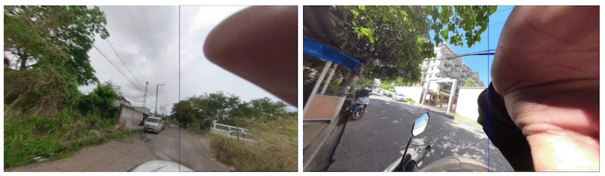
But the main reason was because of a scenario where the recording, at the start or end (but not only), had close-ups of the operator who was checking the camera. This led to images with large regions of interest containing the camera operator’s face – too large to be detected by the model.
An investigation in the dataset structure, by splitting the data into bins based on the bbox sizes (in pixels), made something clear: the dataset was unbalanced.
We made bins for tag sizes with a stride of 100 pixels and went up to the max present in the dataset which accounted for 1 sample of size 2000 pixels. The majority of the labels were small in size and the higher we would go with the size, the less tags we would have. This made it clear that we would need more targeted annotations for our dataset to try to balance it.
All these scenarios required the tagging team to revisit the data multiple times and also change the tagging strategy by including more tags that were considered at a certain limit. It also required them to pay more attention to small details that may have been missed in a previous iteration.
Data Splitting
To better understand the strategy chosen for splitting the data we need to also understand the source of the data. The images come from different devices that are used in different geo locations (different countries) and are from a continuous trip recording. The annotation team used an internal tool to visualise the trips image by image and mark the faces and licence plates present in them. We would then have access to all those images and their respective metadata.
The chosen ratios for splitting are:
Train 70%
Validation 10%
Test 20%
Number of train images
12733
Number of validation images
1682
Number of test images
3221
Number of labeled classes in train set
60630
Number of labeled classes in validation set
7658
Number of of labeled classes in test set
18388
The split is not so trivial as we have some requirements and need to complete some conditions:
An image can have multiple tags from one or both classes but must belong to just one subset.
The tags should be split as close as possible to the desired ratios.
As different images can belong to the same trip in a close geographical relation we need to force them in the same subset, thus avoiding similar tags in train and test subsets, resulting in incorrect evaluations.
Data Augmentation
The application of data augmentation plays a crucial role while training the machine learning model. There are mainly three ways in which data augmentation techniques can be applied. They are:
Offline data augmentation – enriching a dataset by physically multiplying some of its images and applying modifications to them.
Online data augmentation – on the fly modifications of the image during train time with configurable probability for each modification.
Combination of both offline and online data augmentation.
In our case, we are using the third option which is the combination of both.
The first method that contributes to offline augmentation is a method called image view splitting. This is necessary for us due to different image types: perspective camera images, wide field of view images, 360 degree images in equirectangular format. All these formats and field of views with their respective distortions would complicate the data and make it hard for the model to generalise it and also handle different image types that could be added in the future.
For this we defined the concept of image views which are an extracted portion (view) of an image with some predefined properties. For example, the perspective projection of 75 by 75 degrees field of view patches from the original image.
Here we can see a perspective camera image and the image views generated from it:
Figure 5 – Original image
Figure 6 – Two image views generated
The important thing here is that each generated view is an image on its own with the associated tags. They also have an overlapping area so we have a possibility to contain the same tag in two views but from different perspectives. This brings us to an indirect outcome of the first offline augmentation.
The second method for offline augmentation is the oversampling of some of the images (views). As mentioned above, we faced the problem of an unbalanced dataset, specifically we were missing tags that occupied high regions of the image, and even though our tagging teams tried to annotate as many as they could find, these were still scarce.
As our object detection model is an anchor-based detector, we did not even have enough of them to generate the anchor boxes correctly. This could be clearly seen in the accuracy of the previous trained models, as they were performing poorly on bins of big sizes.
By randomly oversampling images that contained big tags, up to a minimum required number, we managed to have better anchors and increase the recall for those scenarios. As described below, the chosen object detector for blurring was YOLOv4 which offers a large variety of online augmentations. The online augmentations used are saturation, exposure, hue, flip and mosaic.
Model
As of summer of 2021, the “to go” solution for object detection in images are convolutional neural networks (CNN), being a mature solution able to fulfil the needs efficiently.
Architecture
Most CNN based object detectors have three main parts: Backbone, Neck and (Dense or Sparse Prediction) Heads. From the input image, the backbone extracts features which can be combined in the neck part to be used by the prediction heads to predict object bounding-boxes and their labels.
Figure 7 – Anatomy of one and two-stage object detectors [1]
The backbone is usually a CNN classification network pretrained on some dataset, like ImageNet-1K. The neck combines features from different layers in order to produce rich representations for both large and small objects. Since the objects to be detected have varying sizes, the topmost features are too coarse to represent smaller objects, so the first CNN based object detectors were fairly weak in detecting small sized objects. The multi-scale, pyramid hierarchy is inherent to CNNs so [2] introduced the Feature Pyramid Network which at marginal costs combines features from multiple scales and makes predictions on them. This or improved variants of this technique is used by most detectors nowadays. The head part does the predictions for bounding boxes and their labels.
YOLO is part of the anchor-based one-stage object detectors family being developed originally in Darknet, an open source neural network framework written in C and CUDA. Back in 2015 it was the first end-to-end differentiable network of this kind that offered a joint learning of object bounding boxes and their labels.
One reason for the big success of newer YOLO versions is that the authors carefully merged new ideas into one architecture, the overall speed of the model being always the north star.
YOLOv4 introduces several changes to its v3 predecessor:
Backbone – CSPDarknet53: YOLOv3 Darknet53 backbone was modified to use Cross Stage Partial Network (CSPNet [5]) strategy, which aims to achieve richer gradient combinations by letting the gradient flow propagate through different network paths.
Multiple configurable augmentation and loss function types, so called “Bag of freebies”, which by changing the training strategy can yield higher accuracy without impacting the inference time.
Configurable necks and different activation functions, they call “Bag of specials”.
Insights
For this task, we found that YOLOv4 gave a good compromise between speed and accuracy as it has doubled the speed of a more accurate two-stage detector while maintaining a very good overall precision/recall. For blurring, the main metric for model selection was the overall recall, while precision and intersection over union (IoU) of the predicted box comes second as we want to catch all personal data even if some are wrong. Having a multitude of possibilities to configure the detector architecture and train it on our own dataset we conducted several experiments with different configurations for backbones, necks, augmentations and loss functions to come up with our current solution.
We faced challenges in training a good model as the dataset posed a large object/box-level scale imbalance, small objects being over-represented in the dataset. As described in [3] and [4], this affects the scales of the estimated regions and the overall detection performance. In [3] several solutions are proposed for this out of which the SPP [6] blocks and PANet [7] neck used in YOLOv4 together with heavy offline data augmentation increased the performance of the actual model in comparison to the former ones.
As we have evaluated the model; it still has some issues:
Occlusion of the object, either by the camera view, head accessories or other elements:
These cases would need extra annotation in the dataset, just like the faces or licence plates that are really close to the camera and occupy a large region of interest in the image.
As we have a limited number of annotations of close objects to the camera view, the model has incorrectly learnt this, sometimes producing false positives in these situations:
Again, one solution for this would be to include more of these scenarios in the dataset.
What’s Next?
Grab spends a lot of effort ensuring privacy protection for its users so we are always looking for ways to further improve our related models and processes.
As far as efficiency is concerned, there are multiple directions to consider for both the dataset and the model. There are two main factors that drive the costs and the quality: further development of the dataset for additional edge cases (e.g. more training data of people wearing masks) and the operational costs of the model.
As the vast majority of current models require a fully labelled dataset, this puts a large work effort on the Data Entry team before creating a new model. Our dataset increased 4x for it’s third version, still there is room for improvement as described in the Dataset section.
As Grab extends its operation in more cities, new data is collected that has to be processed, this puts an increased focus on running detection models more efficiently.
Directions to pursue to increase our efficiency could be the following:
As plenty of unlabelled data is available from imagery collection, a natural direction to explore is self-supervised visual representation learning techniques to derive a general vision backbone with superior transferring performance for our subsequent tasks as detection, classification.
Experiment with optimisation techniques like pruning and quantisation to get a faster model without sacrificing too much on accuracy.
Explore new architectures: YOLOv5, EfficientDet or Swin-Transformer for Object Detection.
Introduce semi-supervised learning techniques to improve our model performance on the long tail of the data.
References
Alexey Bochkovskiy et al.. YOLOv4: Optimal Speed and Accuracy of Object Detection. arXiv:2004.10934v1
Tsung-Yi Lin et al. Feature Pyramid Networks for Object Detection. arXiv:1612.03144v2
Kemal Oksuz et al.. Imbalance Problems in Object Detection: A Review. arXiv:1909.00169v3
Bharat Singh, Larry S. Davis. An Analysis of Scale Invariance in Object Detection – SNIP. arXiv:1711.08189v2
Chien-Yao Wang et al. CSPNet: A New Backbone that can Enhance Learning Capability of CNN. arXiv:1911.11929v1
Kaiming He et al. Spatial Pyramid Pooling in Deep Convolutional Networks for Visual Recognition. arXiv:1406.4729v4
Shu Liu et al. Path Aggregation Network for Instance Segmentation. arXiv:1803.01534v4
Zhenda Xie et al. Self-Supervised Learning with Swin Transformers. arXiv:2105.04553v2
Join Us
Grab is the leading superapp platform in Southeast Asia, providing everyday services that matter to consumers. More than just a ride-hailing and food delivery app, Grab offers a wide range of on-demand services in the region, including mobility, food, package and grocery delivery services, mobile payments, and financial services across 428 cities in eight countries.
Powered by technology and driven by heart, our mission is to drive Southeast Asia forward by creating economic empowerment for everyone. If this mission speaks to you, join our team today!
At Grab, the Lending team is focused towards building products that help finance various segments of users, such as Passengers, Drivers, or Merchants, based on their needs. The team builds products that enable users to avail funds in a seamless and hassle-free way. In order to achieve this, multiple lending microservices continuously interact with each other. Each microservice handles different responsibilities, such as providing offers, storing user information, disbursing availed amounts to a user’s account, and many more.
In this tech blog, we will discuss what Data and Extract, Transform and Load (ETL) pipelines are and how they are used for processing multiple tasks in the Lending Team at Grab. We will also discuss Ratchet, which is a Go library, that helps us in building data pipelines and handling ETL tasks. Let’s start by covering the basis of Data and ETL pipelines.
What is a Data Pipeline?
A Data pipeline is used to describe a system or a process that moves data from one platform to another. In between platforms, data passes through multiple steps based on defined requirements, where it may be subjected to some kind of modification. All the steps in a Data pipeline are automated, and the output from one step acts as an input for the next step.
An ETL pipeline is a type of Data pipeline that consists of 3 major steps, namely extraction of data from a source, transformation of that data into the desired format, and finally loading the transformed data to the destination. The destination is also known as the sink.
The combination of steps in an ETL pipeline provides functions to assure that the business requirements of the application are achieved.
Let’s briefly look at each of the steps involved in the ETL pipeline.
Data Extraction
Data extraction is used to fetch data from one or multiple sources with ease. The source of data can vary based on the requirement. Some of the commonly used data sources are:
Database
Web-based storage (S3, Google cloud, etc)
Files
User Feeds, CRM, etc.
The data format can also vary from one use case to another. Some of the most commonly used data formats are:
SQL
CSV
JSON
XML
Once data is extracted in the desired format, it is ready to be fed to the transformation step.
Data Transformation
Data transformation involves applying a set of rules and techniques to convert the extracted data into a more meaningful and structured format for use. The extracted data may not always be ready to use. In order to transform the data, one of the following techniques may be used:
Filtering out unnecessary data.
Preprocessing and cleaning of data.
Performing validations on data.
Deriving a new set of data from the existing one.
Aggregating data from multiple sources into a single uniformly structured format.
Data Loading
The final step of an ETL pipeline involves moving the transformed data to a sink where it can be accessed for its use. Based on requirements, a sink can be one of the following:
Database
File
Web-based storage (S3, Google cloud, etc)
An ETL pipeline may or may not have a loadstep based on its requirements. When the transformed data needs to be stored for further use, the loadstep is used to move the transformed data to the storage of choice. However, in some cases, the transformed data may not be needed for any further use and thus, the loadstep can be skipped.
Now that you understand the basics, let’s go over how we, in the Grab Lending team, use an ETL pipeline.
Why Use Ratchet?
At Grab, we use Golang for most of our backend services. Due to Golang’s simplicity, execution speed, and concurrency support, it is a great choice for building data pipeline systems to perform custom ETL tasks.
Given that Ratchet is also written in Go, it allows us to easily build custom data pipelines.
Go channels are connecting each stage of processing, so the syntax for sending data is intuitive for anyone familiar with Go. All data being sent and received is in JSON, providing a nice balance of flexibility and consistency.
Utilising Ratchet for ETL Tasks
We use Ratchet for multiple ETL tasks like batch processing, restructuring and rescheduling of loans, creating user profiles, and so on. One of the backend services, named Azkaban, is responsible for handling various ETL tasks.
Ratchet uses Data Processors for building a pipeline consisting of multiple stages. Data Processors each run in their own goroutine so all of the data is processed concurrently. Data Processors are organised into stages, and those stages are run within a pipeline. For building an ETL pipeline, each of the three steps (Extract, Transform and Load) use a Data Processor for implementation. Ratchet provides a set of built-in, useful Data Processors, while also providing an interface to implement your own. Usually, the transform stage uses a Custom Data Processor.
Let’s take a look at one of these tasks to understand how we utilise Ratchet for processing an ETL task.
Whitelisting Merchants Through ETL Pipelines
Whitelisting essentially means making the product available to the user by mapping an offer to the user ID. If a merchant in Thailand receives an option to opt for Cash Loan, it is done by whitelisting that merchant. In order to whitelist our merchants, our Operations team uses an internal portal to upload a CSV file with the user IDs of the merchants and other required information. This CSV file is generated by our internal Data and Risk team and handed over to the Operations team. Once the CSV file is uploaded, the user IDs present in the file are whitelisted within minutes. However, a lot of work goes in the background to make this possible.
Data Extraction
Once the Operations team uploads the CSV containing a list of merchant users to be whitelisted, the file is stored in S3 and an entry is created on the Azkaban service with the document ID of the uploaded file.
File upload by Operations team
The data extraction step makes use of a Custom CSV Data Processor that uses the document ID to first create a PreSignedUrl and then uses it to fetch the data from S3. The data extracted is in bytes and we use commas as the delimiter to format the CSV data.
Data Transformation
In order to transform the data, we define a Custom Data Processor that we call a Transformer for each ETL pipeline. Transformers are responsible for applying all necessary transformations to the data before it is ready for loading. The transformations applied in the merchant whitelisting transformers are:
Convert data from bytes to struct.
Check for presence of all mandatory fields in the received data.
Perform validation on the data received.
Make API calls to external microservices for whitelisting the merchant.
As mentioned earlier, the CSV file is uploaded manually by the Operations team. Since this is a manual process, it is prone to human errors. Validation of data in the data transformation step helps avoid these errors and not propagate them further up the pipeline. Since CSV data consists of multiple rows, each row passes through all the steps mentioned above.
Data Loading
Whenever the merchants are whitelisted, we don’t need to store the transformed data. As a result, we don’t have a loadstep for this ETL task, so we just use an Empty Data Processor. However, this is just one of many use cases that we have. In cases where the transformed data needs to be stored for further use, the loadstep will have a Custom Data Processor, which will be responsible for storing the data.
Connecting All Stages
After defining our Data Processors for each of the steps in the ETL pipeline, the final piece is to connect all the stages together. As stated earlier, the ETL tasks have different ETL pipelines and each ETL pipeline consists of 3 stages defined by their Data Processors.
In order to connect these 3 stages, we define a Job Processor for each ETL pipeline. A Job Processor represents the entire ETL pipeline and encompasses Data Processors for each of the 3 stages. Each Job Processor implements the following methods:
SetSource: Assigns the Data Processor for the Extraction stage.
SetTransformer: Assigns the Data Processor for the Transformation stage.
SetDestination: Assigns the Data Processor for the Load stage.
Execute: Runs the ETL pipeline.
Job processors containing Data Processor for each stage in ETL
When the Azkaban service is initialised, we run the SetSource(), SetTransformer() and SetDestination() methods for each of the Job Processors defined. When an ETL task is triggered, the Execute() method of the corresponding Job Processor is run. This triggers the ETL pipeline and gradually runs the 3 stages of ETL pipeline. For each stage, the Data Processor assigned during initialisation is executed.
Conclusion
ETL pipelines help us in streamlining various tasks in our team. As showcased through the example in the above section, an ETL pipeline breaks a task into multiple stages and divides the responsibilities across these stages.
In cases where a task fails in the middle of the process, ETL pipelines help us determine the cause of the failure quickly and accurately. With ETL pipelines, we have reduced the manual effort required for validating data at each step and avoiding propagation of errors towards the end of the pipeline.
Through the use of ETL pipelines and schedulers, we at Lending have been able to automate the entire pipeline for many tasks to run at scheduled intervals without any manual effort involved at all. This has helped us tremendously in reducing human errors, increasing the throughput of the system and making the backend flow more reliable. As we continue to automate more and more of our tasks that have tightly defined stages, we foresee a growth in our ETL pipelines usage.
Grab is the leading superapp platform in Southeast Asia, providing everyday services that matter to consumers. More than just a ride-hailing and food delivery app, Grab offers a wide range of on-demand services in the region, including mobility, food, package and grocery delivery services, mobile payments, and financial services across 428 cities in eight countries.
Powered by technology and driven by heart, our mission is to drive Southeast Asia forward by creating economic empowerment for everyone. If this mission speaks to you, join our team today!
Data Engineers of Netflix — Interview with Kevin Wylie
This post is part of our “Data Engineers of Netflix” series, where our very own data engineers talk about their journeys to Data Engineering @ Netflix.
Kevin Wylie is a Data Engineer on the Content Data Science and Engineering team. In this post, Kevin talks about his extensive experience in content analytics at Netflix since joining more than 10 years ago.
Kevin grew up in the Washington, DC area, and received his undergraduate degree in Mathematics from Virginia Tech. Before joining Netflix, he worked at MySpace, helping implement page categorization, pathing analysis, sessionization, and more. In his free time he enjoys gardening and playing sports with his 4 kids.
His favorite TV shows: Ozark, Breaking Bad, Black Mirror, Barry, and Chernobyl
Since I joined Netflix back in 2011, my favorite project has been designing and building the first version of our entertainment knowledge graph. The knowledge graph enabled us to better understand the trends of movies, TV shows, talent, and books. Building the knowledge graph offered many interesting technical challenges such as entity resolution (e.g., are these two movie names in different languages really the same?), and distributed graph algorithms in Spark. After we launched the product, analysts and scientists began surfacing new insights that were previously hidden behind difficult-to-use data. The combination of overcoming technical hurdles and creating new opportunities for analysis was rewarding.
Kevin, what drew you to data engineering?
I stumbled into data engineering rather than making an intentional career move into the field. I started my career as an application developer with basic familiarity with SQL. I was later hired into my first purely data gig where I was able to deepen my knowledge of big data. After that, I joined MySpace back at its peak as a data engineer and got my first taste of data warehousing at internet-scale.
What keeps me engaged and enjoying data engineering is giving super-suits and adrenaline shots to analytics engineers and data scientists.
When I make something complex seem simple, or create a clean environment for my stakeholders to explore, research and test, I empower them to do more impactful business-facing work. I like that data engineering isn’t in the limelight, but instead can help create economies of scale for downstream analytics professionals.
What drew you to Netflix?
My wife came across the Netflix job posting in her effort to keep us in Los Angeles near her twin sister’s family. As a big data engineer, I found that there was an enormous amount of opportunity in the Bay Area, but opportunities were more limited in LA where we were based at the time. So the chance to work at Netflix was exciting because it allowed me to live closer to family, but also provided the kind of data scale that was most common for Bay Area companies.
The company was intriguing to begin with, but I knew nothing of the talent, culture, or leadership’s vision. I had been a happy subscriber of Netflix’s DVD-rental program (no late fees!) for years.
After interviewing, it became clear to me that this company culture was different than any I had experienced.
I was especially intrigued by the trust they put in each employee. Speaking with fellow employees allowed me to get a sense for the kinds of people Netflix hires. The interview panel’s humility, curiosity and business acumen was quite impressive and inspired me to join them.
I was also excited by the prospect of doing analytics on movies and TV shows, which was something I enjoyed exploring outside of work. It seemed fortuitous that the area of analytics that I’d be working in would align so well with my hobbies and interests!
Kevin, you’ve been at Netflix for over 10 years now, which is pretty incredible. Over the course of your time here, how has your role evolved?
When I joined Netflix back in 2011, our content analytics team was just 3 people. We had a small office in Los Angeles focused on content, and significantly more employees at the headquarters in Los Gatos. The company was primarily thought of as a tech company.
At the time, the data engineering team mainly used a data warehouse ETL tool called Ab Initio, and an MPP (Massively Parallel Processing) database for warehousing. Both were appliances located in our own data center. Hadoop was being lightly tested, but only in a few high-scale areas.
Fast forward 10 years, and Netflix is now the leading streaming entertainment service — serving members in over 190 countries. In the data engineering space, very little of the same technology remains. Our data centers are retired, Hadoop has been replaced by Spark, Ab Initio and our MPP database no longer fits our big data ecosystem.
In addition to the company and tech shifting, my role has evolved quite a bit as our company has grown. When we were a smaller company, the ability to span multiple functions was valued for agility and speed of delivery. The sooner we could ingest new data and create dashboards and reports for non-technical users to explore and analyze, the sooner we could deliver results. But now, we have a much more mature business, and many more analytics stakeholders that we serve.
For a few years, I was in a management role, leading a great team of people with diverse backgrounds and skill sets. However, I missed creating data products with my own hands so I wanted to step back into a hands-on engineering role. My boss was gracious enough to let me make this change and focus on impacting the business as an individual contributor.
As I think about my future at Netflix, what motivates me is largely the same as what I’ve always been passionate about. I want to make the lives of data consumers easier and to enable them to be more impactful. As the company scales and as we continue to invest in storytelling, the opportunity grows for me to influence these decisions through better access to information and insights. The biggest impact I can make as a data engineer is creating economies of scale by producing data products that will serve a diverse set of use cases and stakeholders.
If I can build beautifully simple data products for analytics engineers, data scientists, and analysts, we can all get better at Netflix’s goal: entertaining the world.
Learning more
Interested in learning more about data roles at Netflix? You’re in the right place! Keep an eye out for our open roles in Data Science and Engineering by visiting our jobs site here. Our culture is key to our impact and growth: read about it here. To learn more about our Data Engineers, check out our chats with Dhevi Rajendran and Samuel Setegne.
Last night’s Italy-England match was a nail-biter. 1-1 at full time, 1-1 at the end of extra time, and then an amazing penalty shootout with incredible goalkeeping by Pickford and Donnarumma.
Cloudflare has been publishing statistics about all the teams involved in EURO 2020 and traffic to betting websites, sports newspapers, streaming services and sponsors. Here’s a quick look at some specific highlights from England’s and Italy’s EURO 2020.
Two interesting peaks show up in UK visits to sports newspapers: the day after England-Germany and today after England’s defeat. Looks like fans are hungry for analysis and news beyond the goals. You can see all the data on the dedicated England EURO 2020 page on Cloudflare Radar.
But it was a quiet morning for the websites of the England team’s sponsors.
Turning to the winners, we can see that Italian readers are even more interested in knowing more about their team’s success.
And this enthusiasm spills over into visits to the Italian team’s sponsors.
You can follow along on the dedicated Cloudflare Radar page for Italy in EURO 2020.
Visit Cloudflare Radar for information on global Internet trends, trending domains, attacks and usage statistics.
Data Engineers of Netflix — Interview with Dhevi Rajendran
Dhevi Rajendran
This post is part of our “Data Engineers of Netflix” interview series, where our very own data engineers talk about their journeys to Data Engineering @ Netflix.
Dhevi Rajendran is a Data Engineer on the Growth Data Science and Engineering team. Dhevi joined Netflix in July 2020 and is one of many Data Engineers who have onboarded remotely during the pandemic. In this post, Dhevi talks about her passion for data engineering and taking on a new role during the pandemic.
Before Netflix, Dhevi was a software engineer at Two Sigma, where she was most recently on a data engineering team responsible for bringing in datasets from a variety of different sources for research and trading purposes. In her free time, she enjoys drawing, doing puzzles, reading, writing, traveling, cooking, and learning new things.
Her favorite TV shows: Atlanta, Barry, Better Call Saul, Breaking Bad, Dark, Fargo, Succession, The Killing
Her favorite movies: Das Leben der Anderen, Good Will Hunting, Intouchables, Mother, Spirited Away, The Dark Knight, The Truman Show, Up
Dhevi, so what got you into data engineering?
While my background has mostly been in backend software engineering, I was most recently doing backend work in the data space prior to Netflix. One great thing about working with data is the impact you can create as an engineer.
At Netflix, the work that data engineers do to produce data in a robust, scalable way is incredibly important to provide the best experience to our members as they interact with our service.
Beyond the really interesting technical challenges that come with working with big data, there are lots of opportunities to think about higher-level domain challenges as a data engineer. In college, I had done human-computer interaction research on subtitles for the Deaf and hard-of-hearing as well as computational genomics research on Alzheimer’s disease. I’ve always enjoyed learning about new areas and combining this knowledge with my technical skills to solve real-world problems.
What drew you to Netflix?
Netflix’s mission and its culture primarily drew me to Netflix. I liked the idea of being a part of a company that brings joy to so many members around the world with an incredibly powerful platform for their stories to be heard. The blend of creativity and a strong engineering culture at Netflix really appealed to me.
The culture was also something that piqued my interest. I was pretty skeptical of Netflix’s culture memo at first. Many companies have lofty ideals that don’t necessarily translate into the reality of the company culture, so I was surprised to see how consistently the culture memo aligns with the actual culture at the company. I’ve found the culture of freedom and responsibility empowering.
Rather than the typical top-down approach many companies use, Netflix trusts each person to make the right decisions for the company by using their deep knowledge of the problems they’re solving along with the context they gather from their leaders and stakeholders.
This means a lot less red tape, a lot less friction, and a lot more freedom for everyone at the company to do what’s best for the business. I also really appreciate the amount of visibility and input we get into broader strategic decisions that the company makes.
Finally, I was also really excited about joining the Growth Data Engineering team! My team is responsible for building data products relating to how we connect with our new members around the world, which is high-impact and has far-reaching global significance. I love that I get to help Netflix connect with new members around the world and help shape the first impression we make on them.
What is your favorite project or a project that you’re particularly proud of?
I have been primarily involved in the payments space. Not a project per se, but one of the things I’ve enjoyed being involved in is the cross-functional meetings with peers and stakeholders who are working in the payments space. These meetings include product managers, designers, consumer insights researchers, software engineers, data scientists, and people in a wide variety of other roles.
I love that I get to work cross-functionally with such a diverse group of people looking at the same set of problems from a variety of unique perspectives.
In addition to my day-to-day technical work, these meetings have provided me with the opportunity to be involved in the high-level product, design, and strategic discussions, which I value. Through these cross-functional efforts, I’ve also really gotten to learn and appreciate the nuances of payments. From using credit cards (which are fairly common in the US but not as widely adopted outside the US) to physically paying in person, members in different countries prefer to pay for our subscription in a wide variety of ways. It’s incredible to see the thoughtful and deeply member-driven approach we use to think about something as seemingly routine, straightforward, and often taken for granted as payments.
What was it like taking on a new role during the pandemic?
First off, I feel very lucky to have found a new role in this very difficult period. With the amount of change and uncertainty, the past year brought, it somehow felt both fitting and imprudent to voluntarily add a career change to the mix. The prospect was daunting at first. I knew there would be a bunch for me to learn coming into Netflix, considering that I hadn’t worked with the technologies my team uses (primarily Scala and Spark). Looking back now, I’m incredibly grateful for the opportunity and glad that I took it. I’ve already learned so much in the past six months and am excited about how much more I can learn and the impact I can make going forward.
Onboarding remotely has been a unique experience as well. Building relationships and gathering broader context are more difficult right now. I’ve found that I’ve learned to be more proactive and actively seek out opportunities to get to know people and the business, whether through setting up coffee chats, reading memos, or attending meetings covering topics I want to learn more about. I still haven’t met anyone I work with in person, but my teammates, my manager, and people across the company have been really helpful throughout the onboarding process.
It’s been incredible to see how gracious people are with their time and knowledge. The amount of empathy and understanding people have shown to each other, including to those who are new to the company, has made taking the leap and joining Netflix a positive experience.
Learning more
Interested in learning more about data roles at Netflix? You’re in the right place! Keep an eye out for our open roles in Data Science and Engineering here. Our culture is key to our impact and growth: read about it here.
Data is the lifeblood of Grab and the insights we gain from it drive all the most critical business decisions made by Grabbers and our leaders every day.
Grab’s Data Engineering (DE) team is responsible for maintaining the data platform, which consists of data pipelines, job schedulers, and the query/computation engines that are the key components for generating insights from data. SQL is the core language for analytics at Grab and as of early 2020, our Presto platform serves about 200 user groups that add up to 500 users who run 350,000 queries every day. These queries span across 10,000 tables that process up to 1PB of data daily.
In 2016, we started the DataGateway project to enable us to manage data access for the hundreds of Grabbers who needed access to Presto for their work. Since then, DataGateway has grown to become much more than just an access control mechanism for Presto. In this blog, we want to share what we’ve achieved since the initial launch of the project.
The problems we wanted to solve
As we were reviewing the key challenges around data access in Grab and assessing possible solutions, we came up with this prioritized list of user requirements we wanted to work on:
Use a single endpoint to serve everyone.
Manage user access to clusters, schemas, tables, and fields.
Provide seamless user experience when presto clusters are scaled up/down, in/out, or provisioned/decommissioned.
Capture audit trail of user activities.
To provide Grabbers with the critical need of interactive querying, as well as performing extract, transform, load (ETL) jobs, we evaluated several technologies. Presto was among the ones we evaluated, and was what we eventually chose although it didn’t meet all of our requirements out of the box. In order to address these gaps, we came up with the idea of a security gateway for the Presto compute engine that could also act as a load balancer/proxy, this is how we ended up creating the DataGateway.
DataGateway is a service that sits between clients and Presto clusters. It is essentially a smart HTTP proxy server that is an abstraction layer on top of the Presto clusters that handles the following actions:
Parse incoming SQL statements to get requested schemas, tables, and fields.
Manage user Access Control List (ACL) to limit users’ data access by checking against the SQL parsing results.
Manage users’ cluster access.
Redirect users’ traffic to the authorized clusters.
Show meaningful error messages to users whenever the query is rejected or exceptions from clusters are encountered.
Anatomy of DataGateway
The DataGateway’s key components are as follows:
API Service
SQL Parser
Auth framework
Administration UI
We leveraged Kubernetes to run all these components as microservices.
Figure 1. DataGateway Key Components
API Service
This is the component that manages all users and cluster-facing processes. We integrated this service with the Presto API, which means it appears to be the same as a Presto cluster to a client. It accepts query requests from clients, gets the parsing result and runs authorization from the SQL Parser and the Auth Framework.
If everything is good to go, the API Service forwards queries to the assigned clusters and continues the entire query process.
Auth Framework
This handles both authentication and authorization requests. It stores the ACL of users and communicates with the API Service and the SQL Parser to run the entire authentication process. But why is it a microservice instead of a module in API Service, you ask? It’s because we keep evolving the security checks at Grab to ensure that everything is compliant with our security requirements, especially when dealing with data.
We wanted to make it flexible to fulfill ad-hoc requests from the security team without affecting the API Service. Furthermore, there are different authentication methods out there that we might need to deal with (OAuth2, SSO, you name it). The API Service supports multiple authentication frameworks that enable different authentication methods for different users.
SQL Parser
This is a SQL parsing engine to get schema, tables, and fields by reading SQL statements. Since Presto SQL parsing works differently in each version, we would compile multiple SQL Parsers that are identical to the Presto clusters we run. The SQL Parser becomes the single source of truth.
Admin UI
This is a UI for Presto administrators to manage clusters and user access, as well as to select an authentication framework, making it easier for the administrators to deal with the entire ecosystem.
How we deployed DataGateway using Kubernetes
In the past couple of years, we’ve had significant growth in workloads from analysts and data scientists. As we were very enthusiastic about Kubernetes, DataGateway was chosen as one of the earliest services for deployment in Kubernetes. DataGateway in Kubernetes is known to be highly available and fully scalable to handle traffic from users and systems.
We also tested the HPA feature of Kubernetes, which is a dynamic scaling feature to scale in or out the number of pods based on actual traffic and resource consumption.
Figure 2. DataGateway deployment using Kubernetes
Functionality of DataGateway
This section highlights some of the ways we use DataGateway to manage our Presto ecosystem efficiently.
Restrict users based on Schema/Table level access
In a setup where a Presto cluster is deployed on AWS Amazon Elastic MapReduce (EMR) or Elastic Kubernetes Service (EKS), we configure an IAM role and attach it to the EMR or EKS nodes. The IAM role is set to limit the access to S3 storage. However, the IAM only provides bucket-level and file-level control; it doesn’t meet our requirements to have schema, table, and column-level ACLs. That’s how DataGateway is found useful in such scenarios.
One of the DataGateway services is an SQL Parser. As previously covered, this is a service that parses and digs out schemas and tables involved in a query. The API service receives the parsing result and checks against the ACL of users, and decides whether to allow or reject the query. This is a remarkable improvement in our security control since we now have another layer to restrict access, on top of the S3 storage. We’ve implemented an SQL-based access control down to table level.
As shown in the Figure 3, user A is trying run a SQL statement select * from locations.cities. The SQL Parser reads the statement and tells the API service that user A is trying to read data from the table cities in the schema locations. Then, the API service checks against the ACL of user A. The service finds that user A has only read access to table countries in schema locations. Eventually, the API service denies this attempt because user A doesn’t have read access to table cities in the schema locations.
Figure 3. An example of how to check user access to run SQL statements
The above flow shows an access denied result because the user doesn’t have the appropriate permissions.
Seamless User Experience during the EMR migration
We use AWS EMR to deploy Presto as an SQL query engine since deployment is really easy. However, without DataGateway, any EMR operations such as terminations, new cluster deployment, config changes, and version upgrades, would require quite a bit of user involvement. We would sometimes need users to make changes on their side. For example, request users to change the endpoints to connect to suitable clusters.
With DataGateway, ACLs exist for each of the user accounts. The ACL includes the list of EMR clusters that users are allowed to access. As a Presto access management platform, here the DataGateway redirects user traffics to an appropriate cluster based on the ACL, like a proxy. Users always connect to the same endpoint we offer, which is the DataGateway. To switch over from one cluster to another, we just need to edit the cluster ACL and everything is handled seamlessly.
Figure 4. Cluster switching using DataGateway
Figure 4 highlights the case when we’re switching EMR from one cluster to another. No changes are required from users.
We executed the migration of our entire Presto platform from an AWS EMR instance to another AWS EMR instance using the same methodology. The migrations were executed with little to no disruption for our users. We were able to move 40 clusters with hundreds of users. They were able to issue millions of queries daily in a few phases over a couple of months.
In most cases, users didn’t have to make any changes on their end, they just continued using Presto as usual while we made the changes in the background.
Multi-Cloud Data Lake/Presto Cluster maintenance
Recently, we started to build and maintain data lakes not just in one cloud, but two – in AWS and Azure. Since most end-users are AWS-based, and each team has their own AWS sub-account to run their services and workloads, it would be a nightmare to bridge all the connections and access routes between these two clouds from end-to-end, sub-account by sub-account.
Here, the DataGateway plays the role of the multi-cloud gateway. Since all end-users’ AWS sub-accounts have peered to DataGateway’s network, everything becomes much easier to handle.
For end-users, they retain the same Presto connection profile. The DE team then handles the connection setup from DataGateway to Azure, and also the deployment of Presto clusters in Azure.
When all is set, end-users use the same endpoint to DataGateway. We offer a feature called Cluster Switch that allows users to switch between AWS Presto cluster and Azure Presto Cluster on the fly by filling in parameters on the connection string. This feature allows users to switch to their target Presto cluster without any endpoint changes. The switch works instantly whenever they do the change. That means users can run different queries in different clusters based on their requirements.
This feature has helped the DE team to maintain Presto Cluster easily. We can spin up different Presto clusters for different teams, so that each team has their own query engine to run their queries with dedicated resources.
Figure 5. Sub-account connections and Queries
Figure 5 shows an example of how sub-accounts connect to DataGateway and run queries on resources in different clouds and clusters.
Figure 6. Sample scenario without DataGateway
Figure 6 shows a scenario of what would happen if DataGatway doesn’t exist. Each of the accounts would have to maintain its own connections, Virtual Private Cloud (VPC) peering, and express link to connect to our Presto resources.
Summary
DataGateway is playing a key role in Grab’s entire Presto ecosystem. It helps us manage user access and cluster selections on a single endpoint, ensuring that everyone is running their Presto queries on the same place. It also helps distribute workload to different types and versions of Presto clusters.
When we started to deploy the DataGateway on Kubernetes, our vision for the Presto ecosystem underwent an epic change as it further motivated us to continuously improve. Since then, we’ve had new ideas on deployment method/pipeline, microservice implementations, scaling strategy, resource control, we even made use of Kubernetes and designed an on-demand, container-based Presto cluster provisioning engine. We’ll share this in another engineering blog, so do stay tuned!.
We also made crucial enhancements on data access control as we extended Presto’s access controls down to the schema/table-level.
In day-to-day operations, especially when we started to implement data lake in multiple clouds, DataGateway solved a lot of implementation issues. DataGateway made it simpler to switch a user’s Presto cluster from one cloud to another or allow a user to use a different Presto cluster using parameters. DataGateway allowed us to provide a seamless experience to our users.
Looking forward, we’ve more and more ideas for our Presto ecosystem, such Spark DataGateway or AWS Athena integrations, to keep our data safe at any time and to provide our users with a smoother experience when dealing with data used for analysis or research.
Authored by Vinnson Lee on behalf of the Presto Development Team at Grab – Edwin Law, Qui Hieu Nguyen, Rahul Penti, Wenli Wan, Wang Hui and the Data Engineering Team.
Join us
Grab is more than just the leading ride-hailing and mobile payments platform in Southeast Asia. We use data and technology to improve everything from transportation to payments and financial services across a region of more than 620 million people. We aspire to unlock the true potential of Southeast Asia and look for like-minded individuals to join us on this ride.
If you share our vision of driving South East Asia forward, apply to join our team today.
The collective thoughts of the interwebz
Manage Consent
To provide the best experiences, we use technologies like cookies to store and/or access device information. Consenting to these technologies will allow us to process data such as browsing behavior or unique IDs on this site. Not consenting or withdrawing consent, may adversely affect certain features and functions.
Functional
Always active
The technical storage or access is strictly necessary for the legitimate purpose of enabling the use of a specific service explicitly requested by the subscriber or user, or for the sole purpose of carrying out the transmission of a communication over an electronic communications network.
Preferences
The technical storage or access is necessary for the legitimate purpose of storing preferences that are not requested by the subscriber or user.
Statistics
The technical storage or access that is used exclusively for statistical purposes.The technical storage or access that is used exclusively for anonymous statistical purposes. Without a subpoena, voluntary compliance on the part of your Internet Service Provider, or additional records from a third party, information stored or retrieved for this purpose alone cannot usually be used to identify you.
Marketing
The technical storage or access is required to create user profiles to send advertising, or to track the user on a website or across several websites for similar marketing purposes.
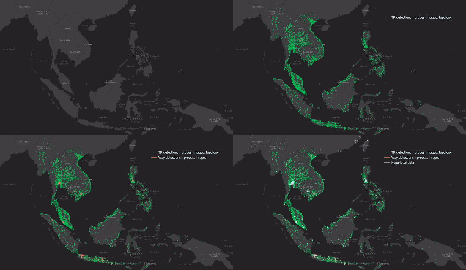

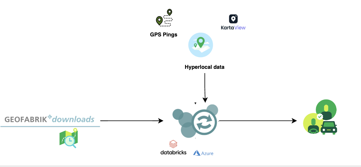
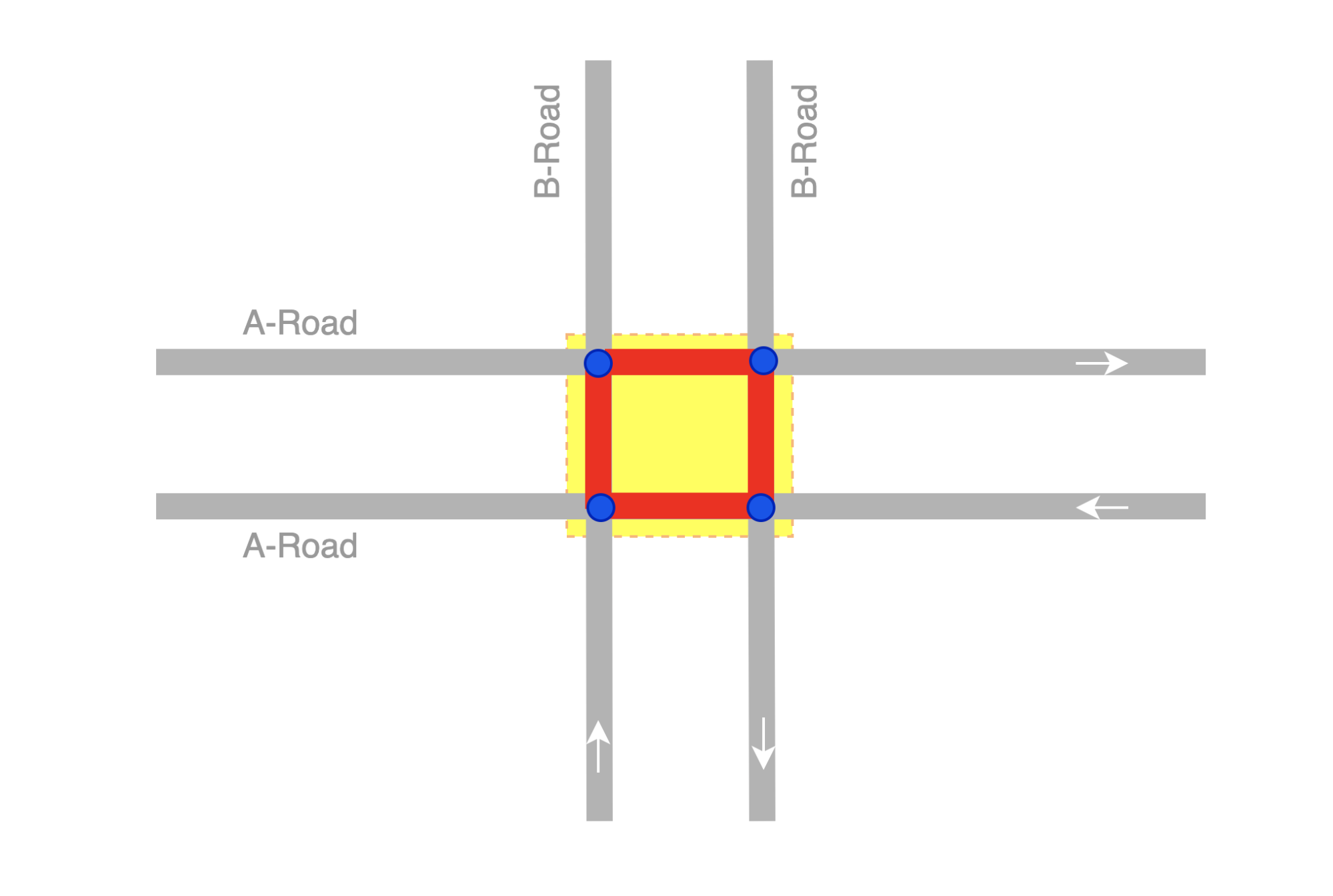
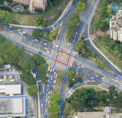
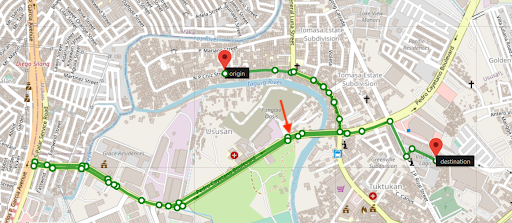
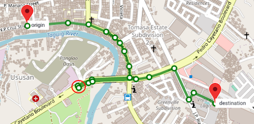

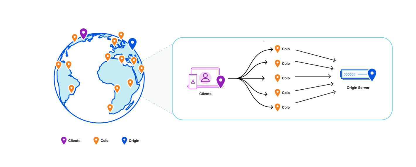
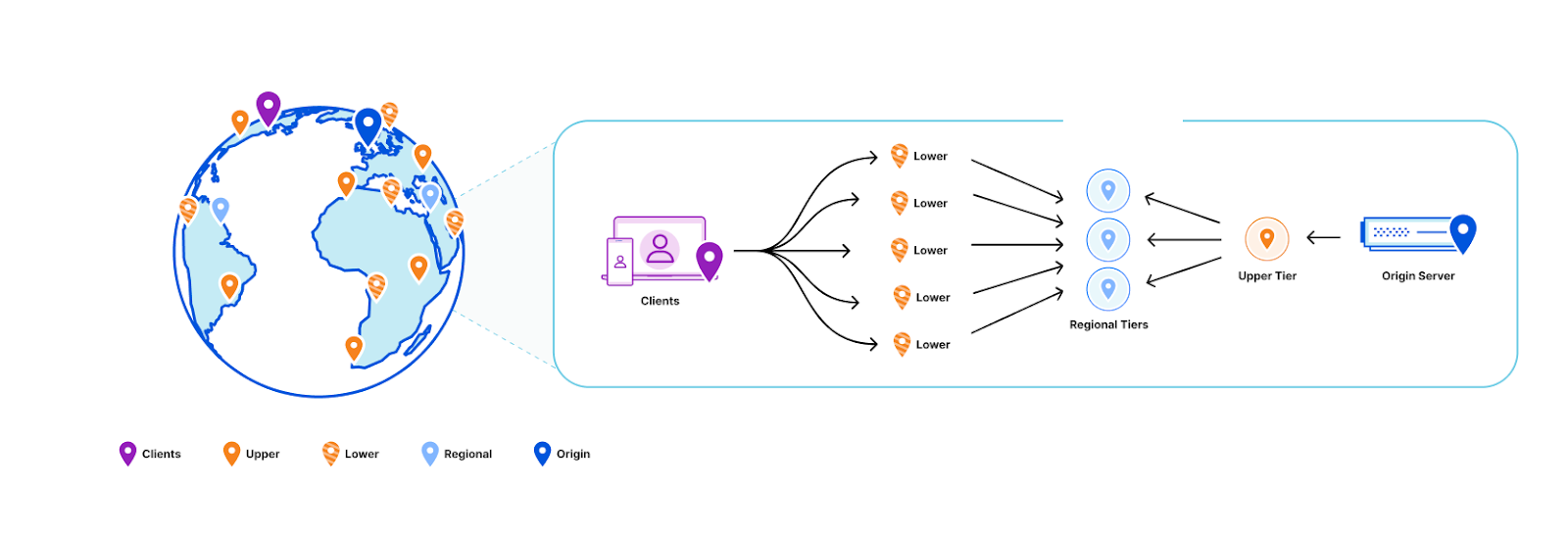
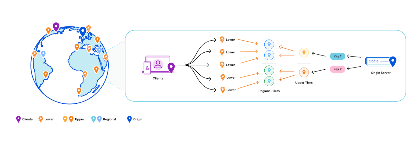
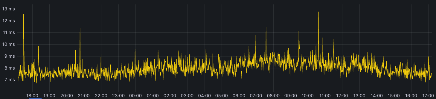




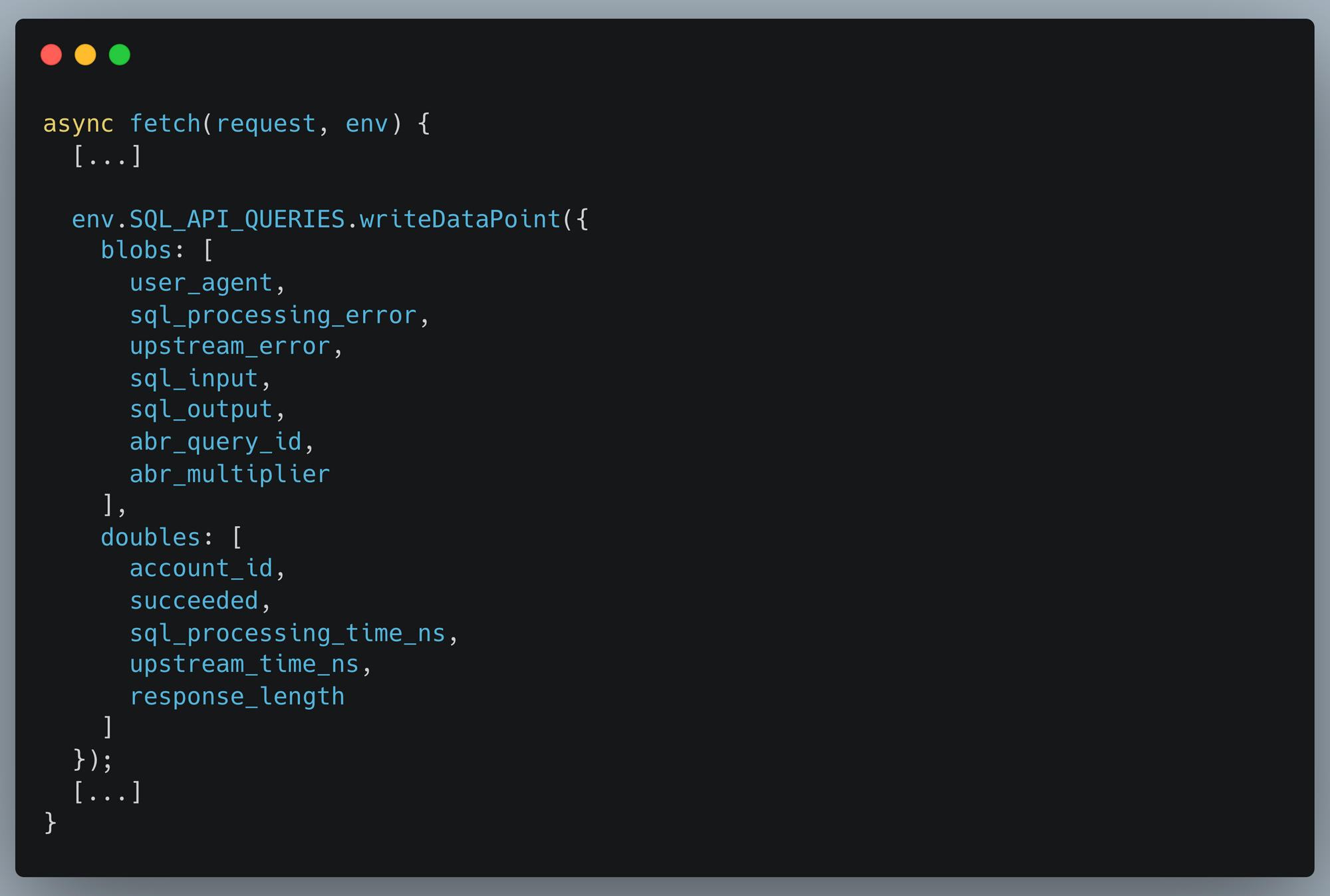
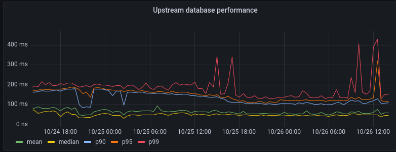
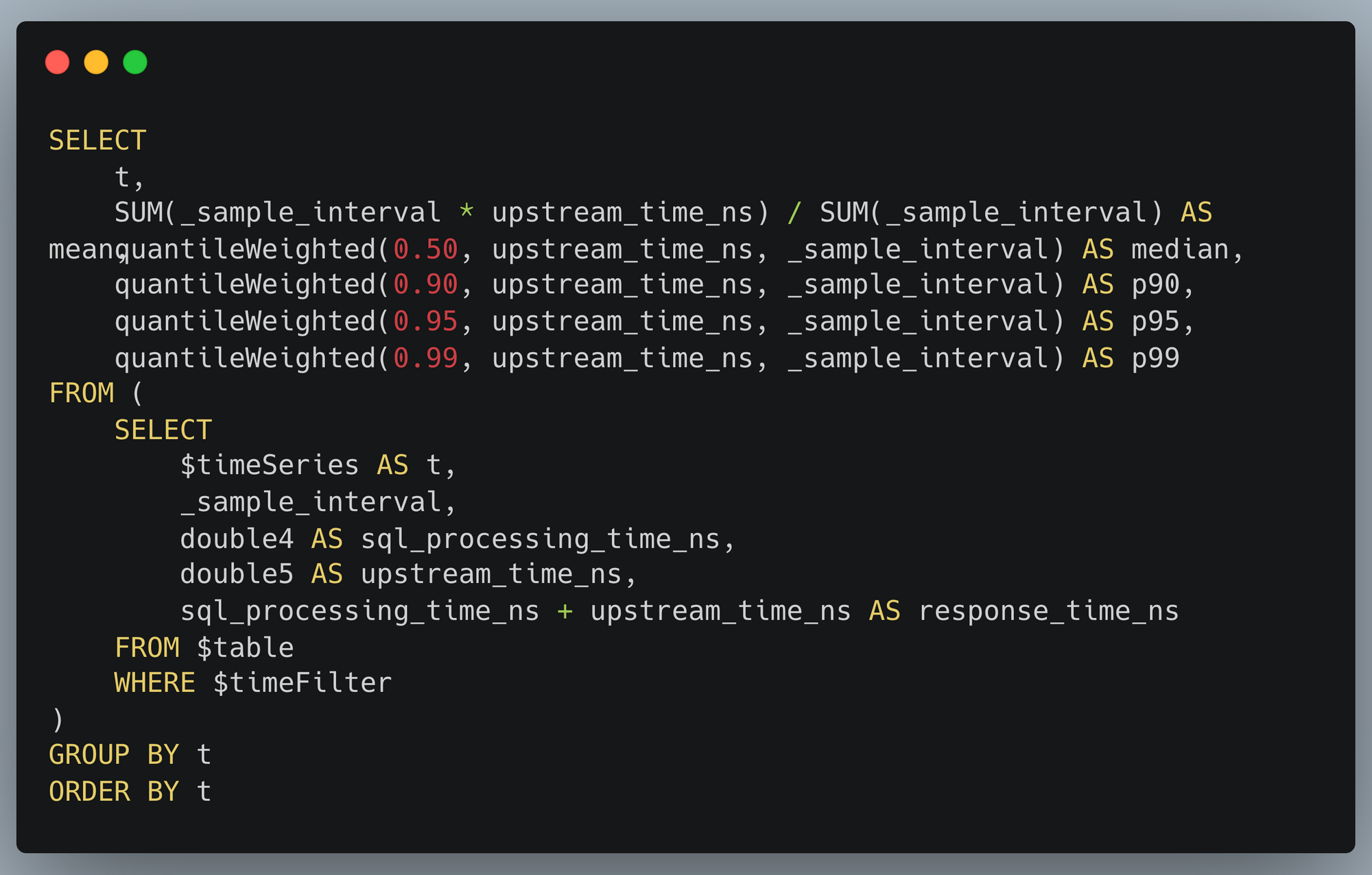
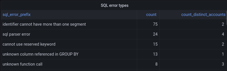
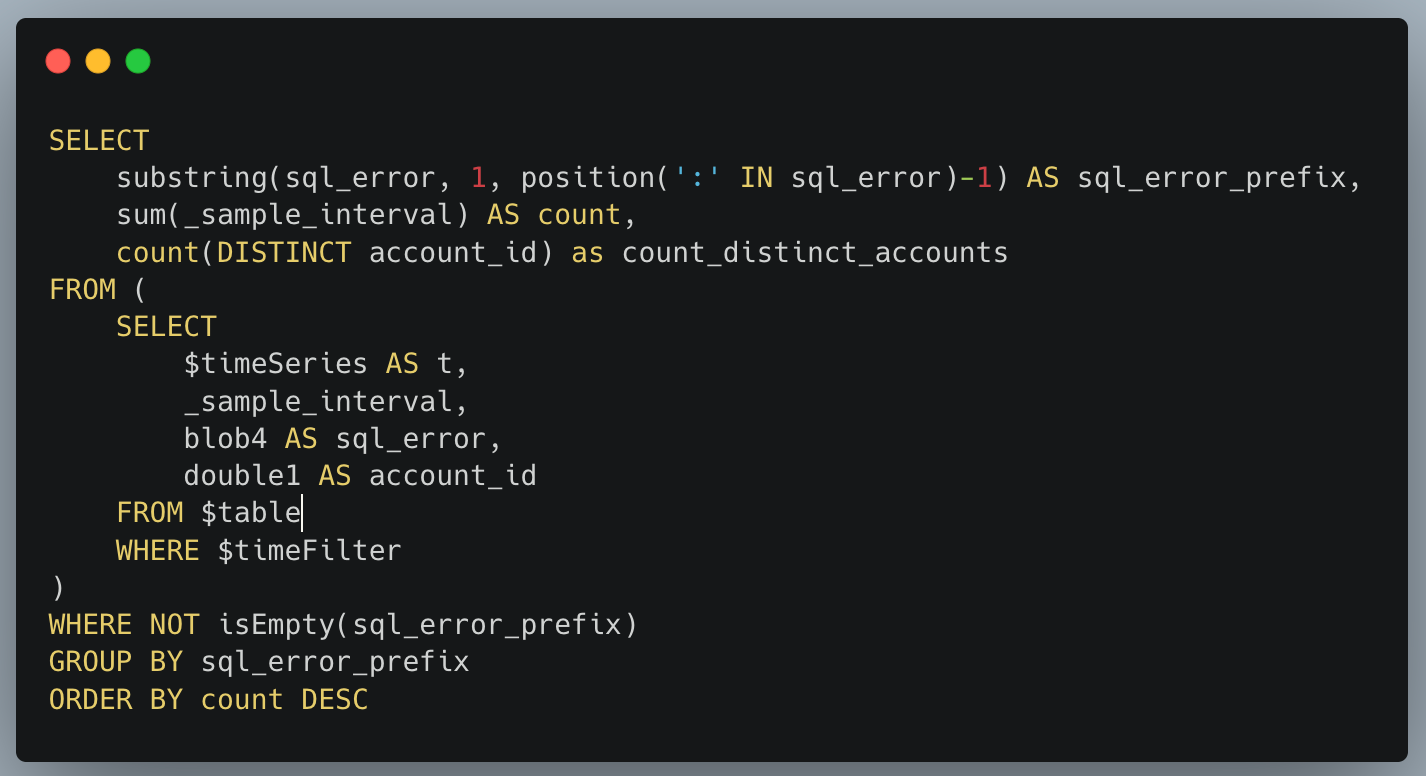
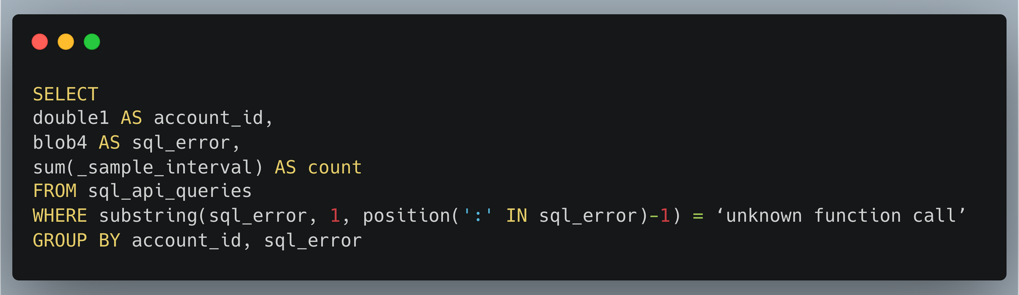
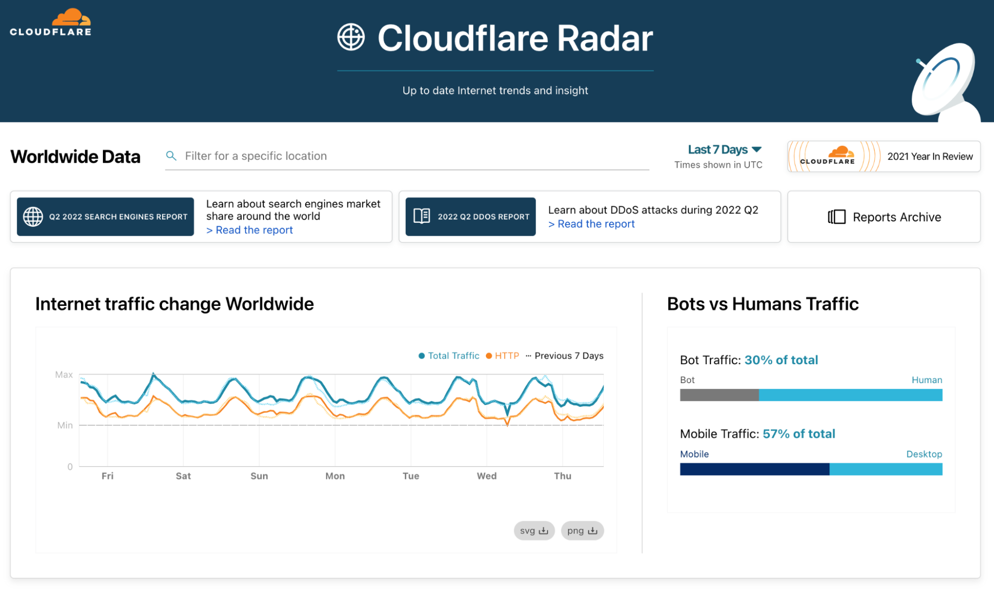
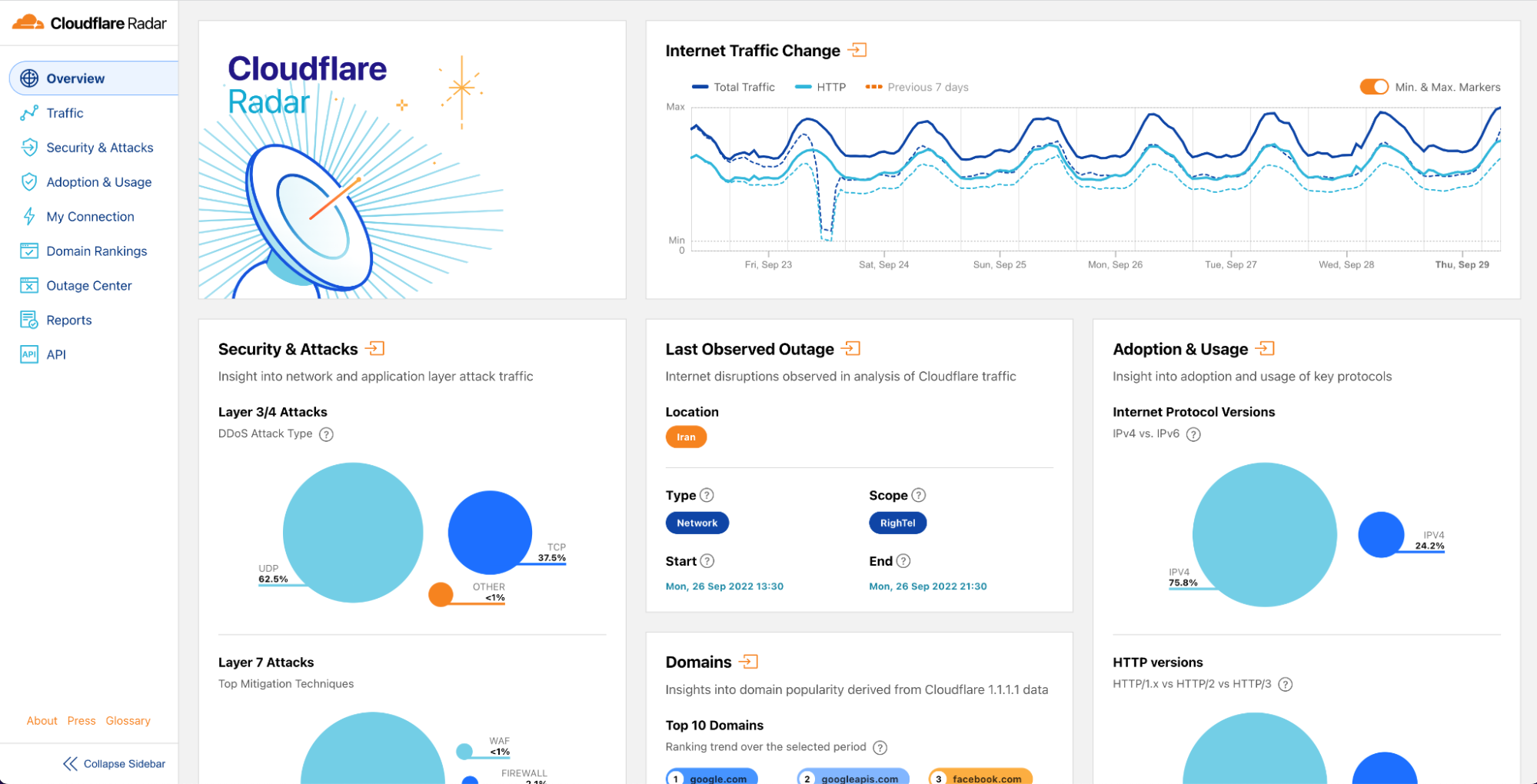
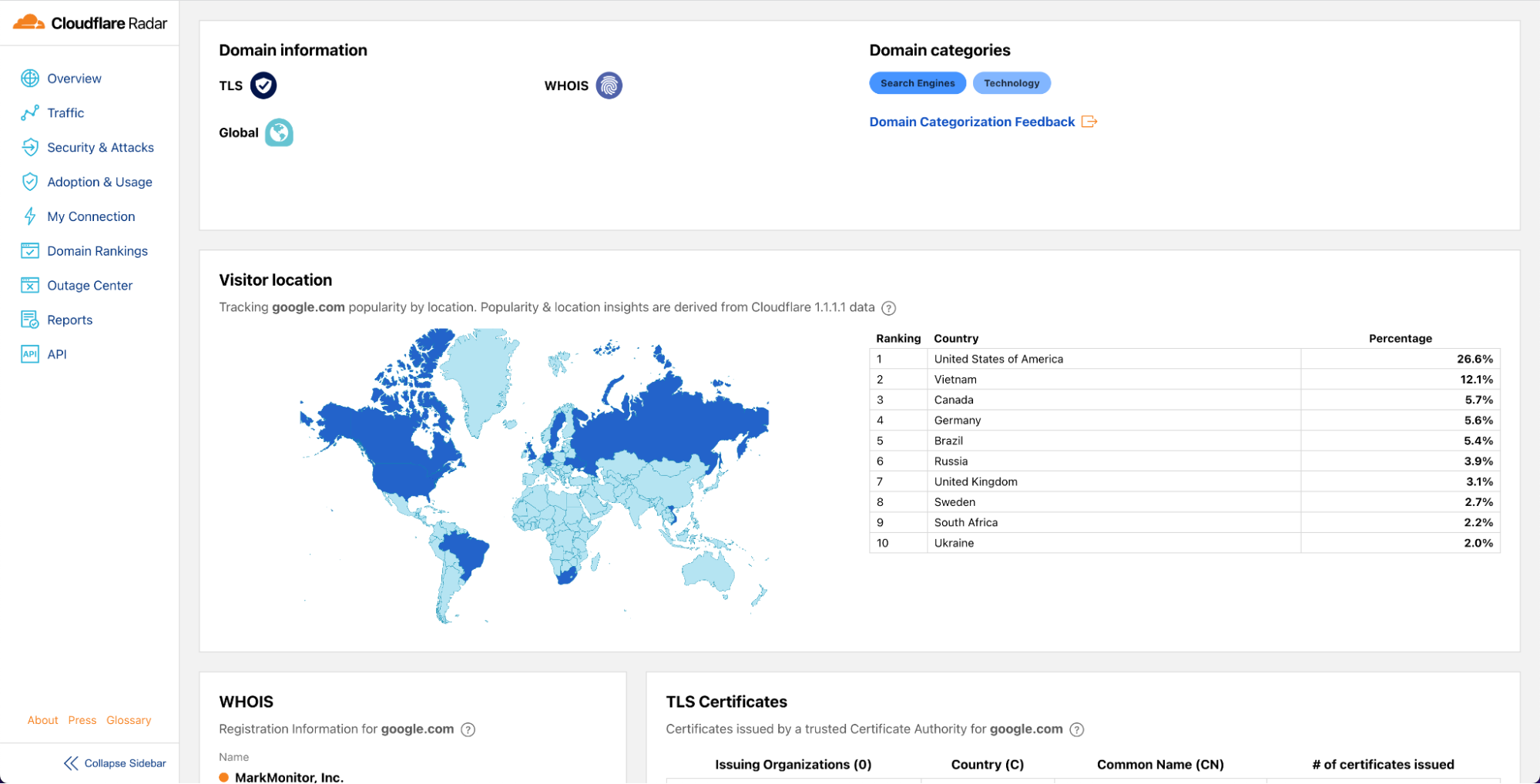
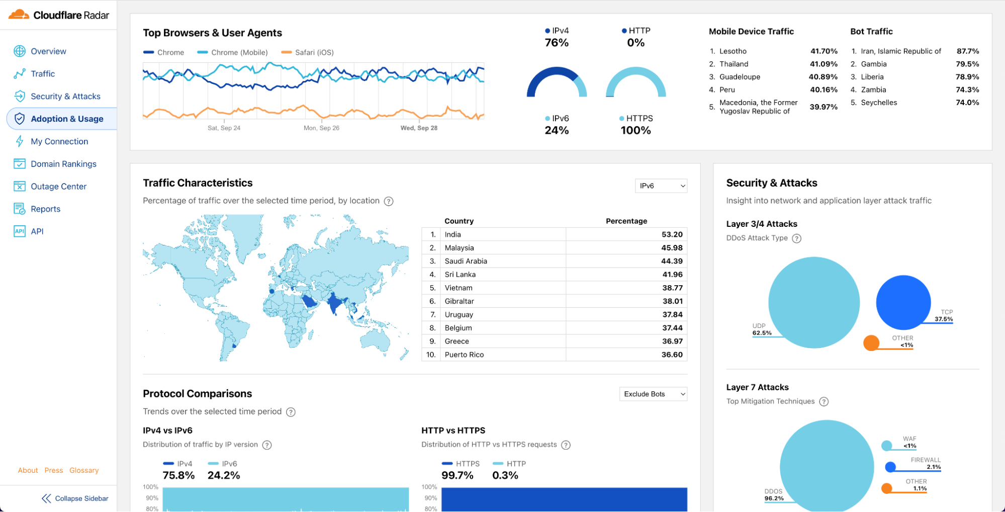
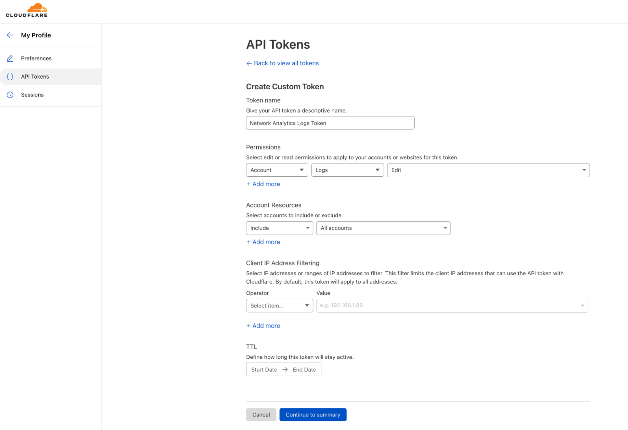

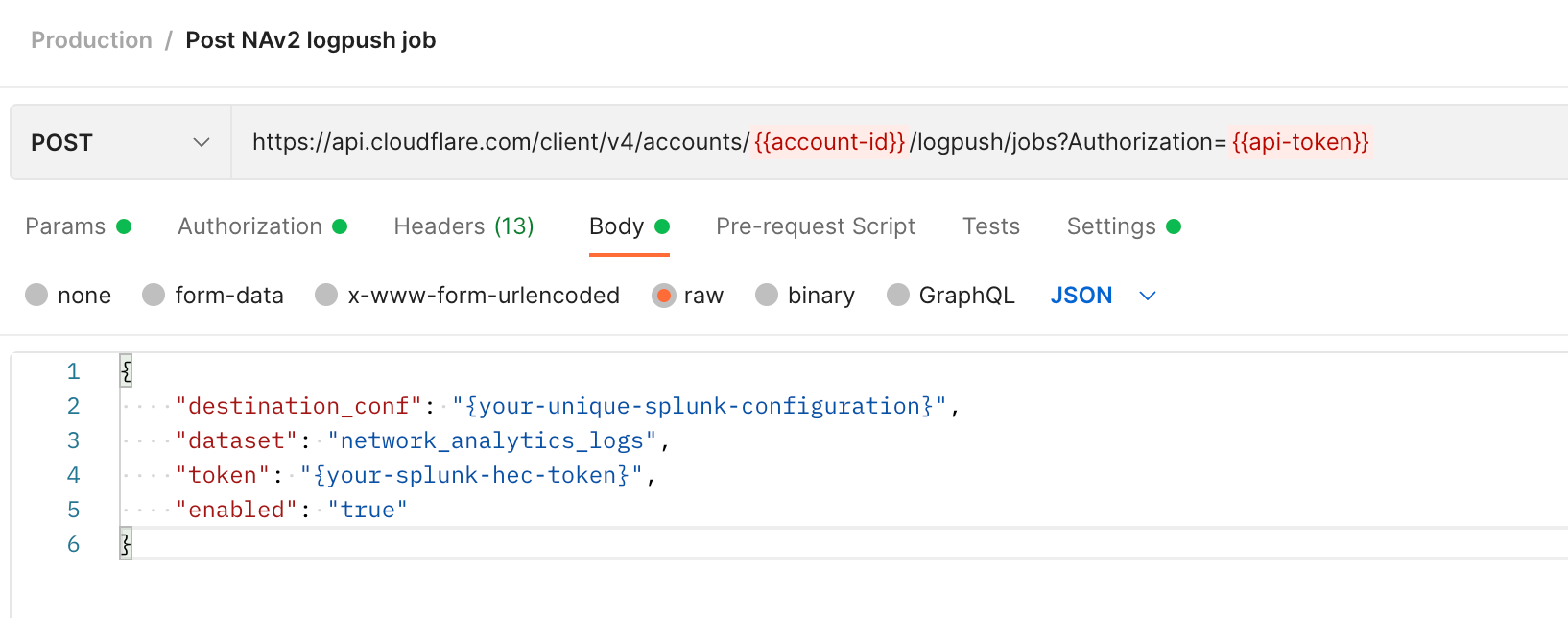
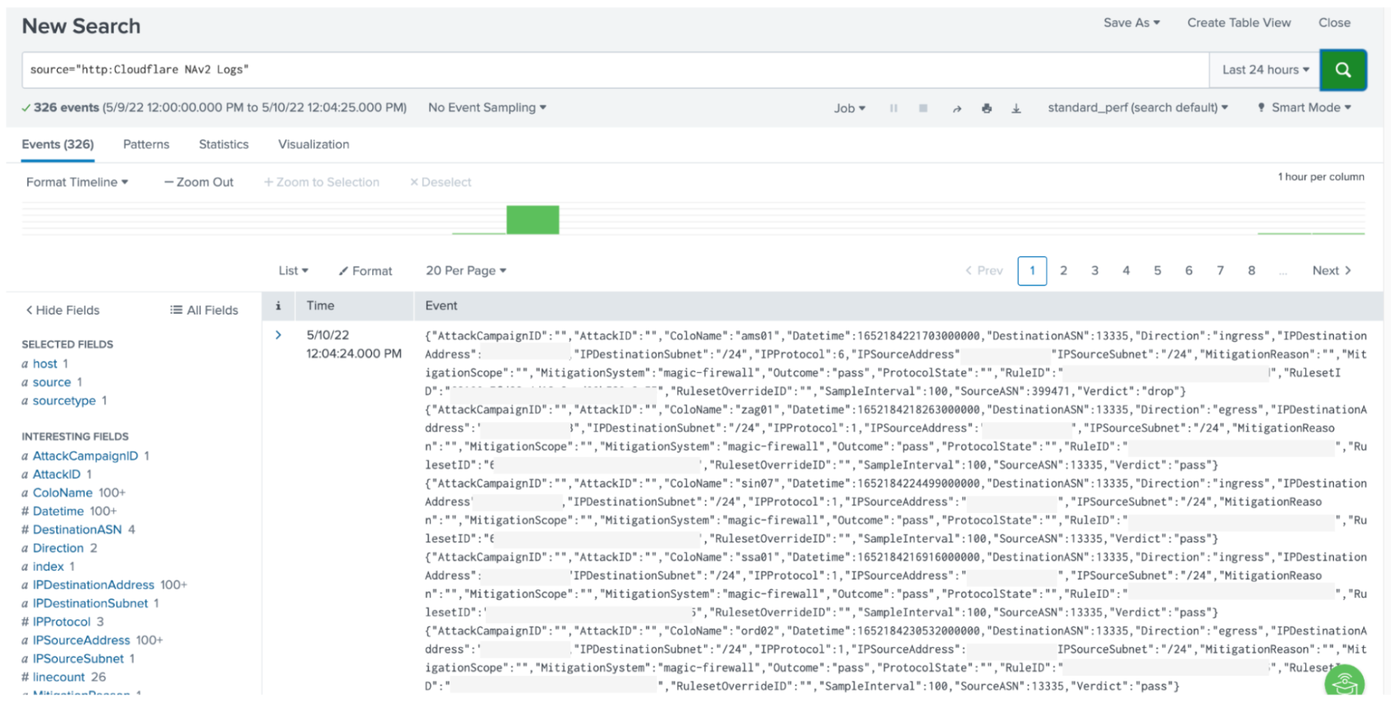
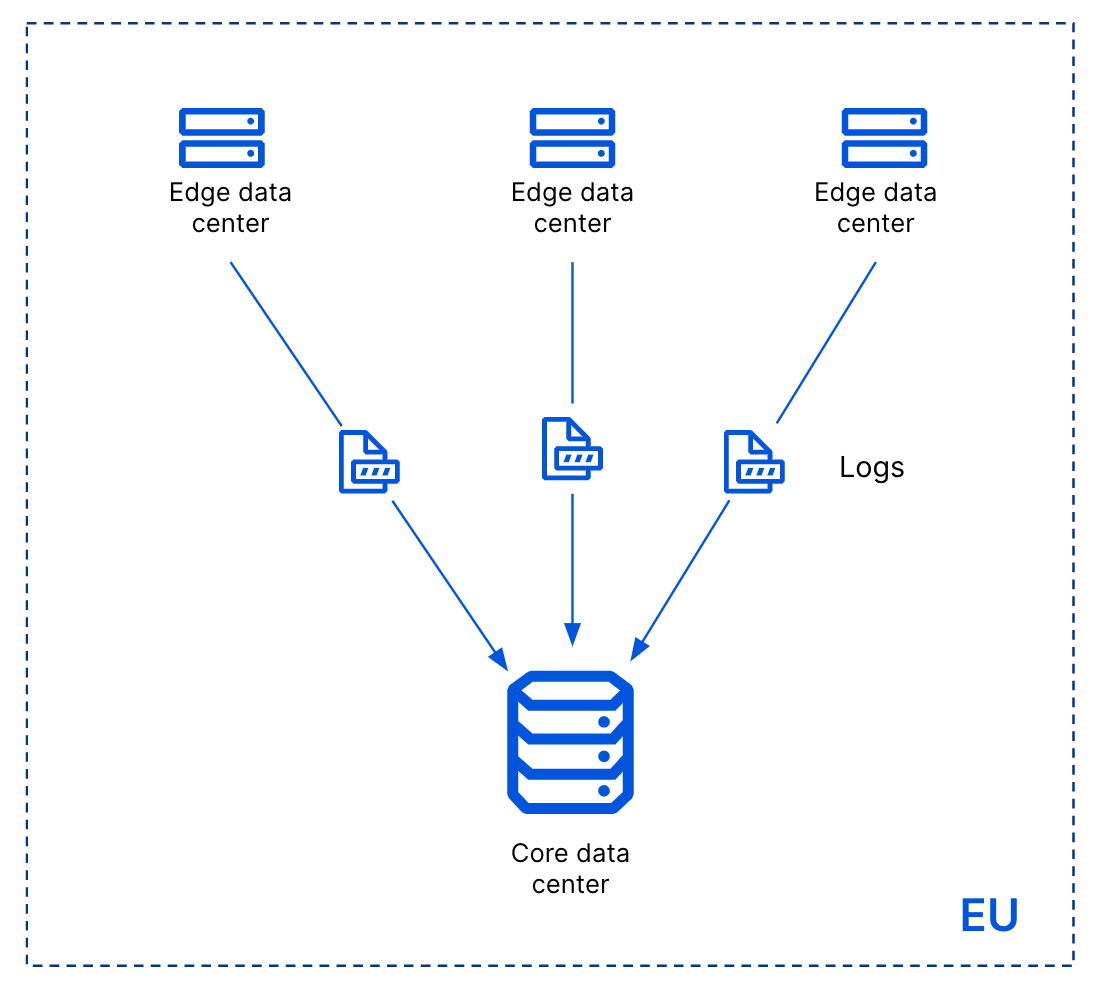


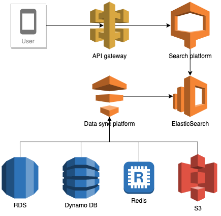

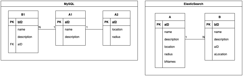
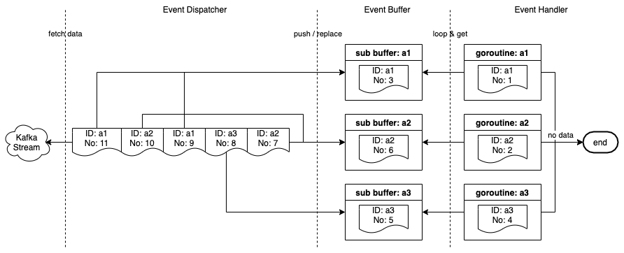
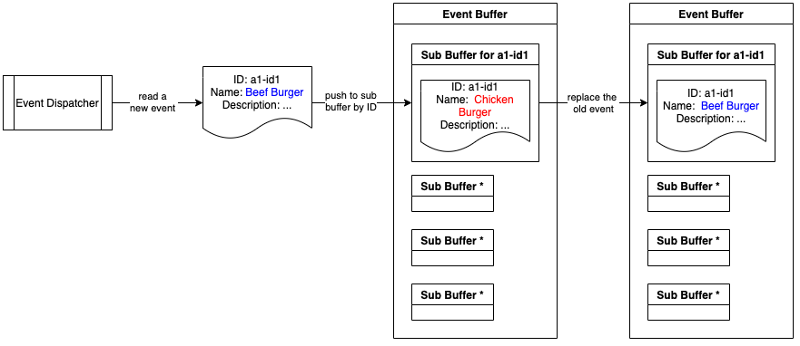
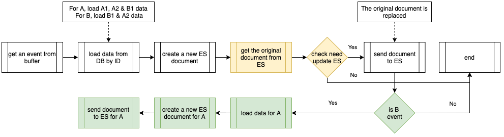
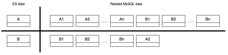
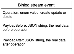
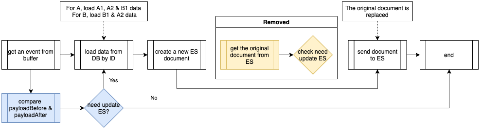
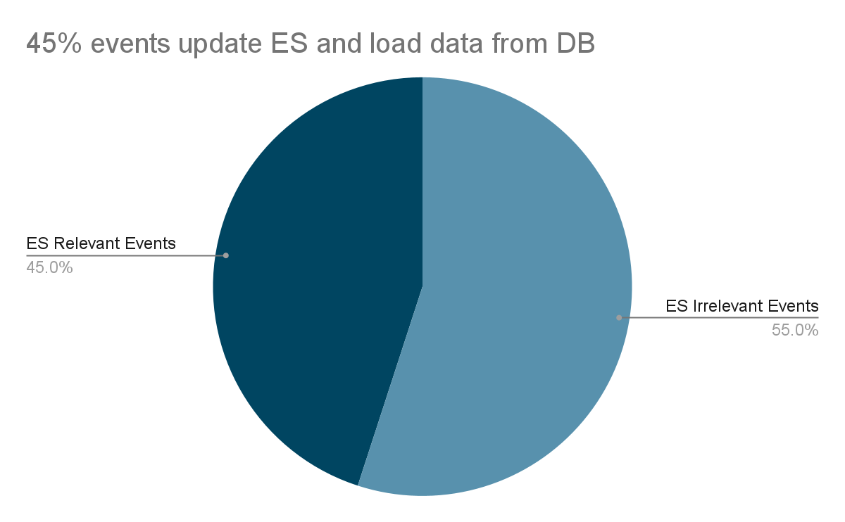
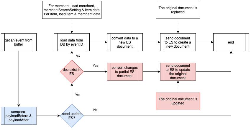
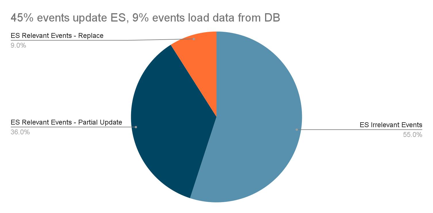
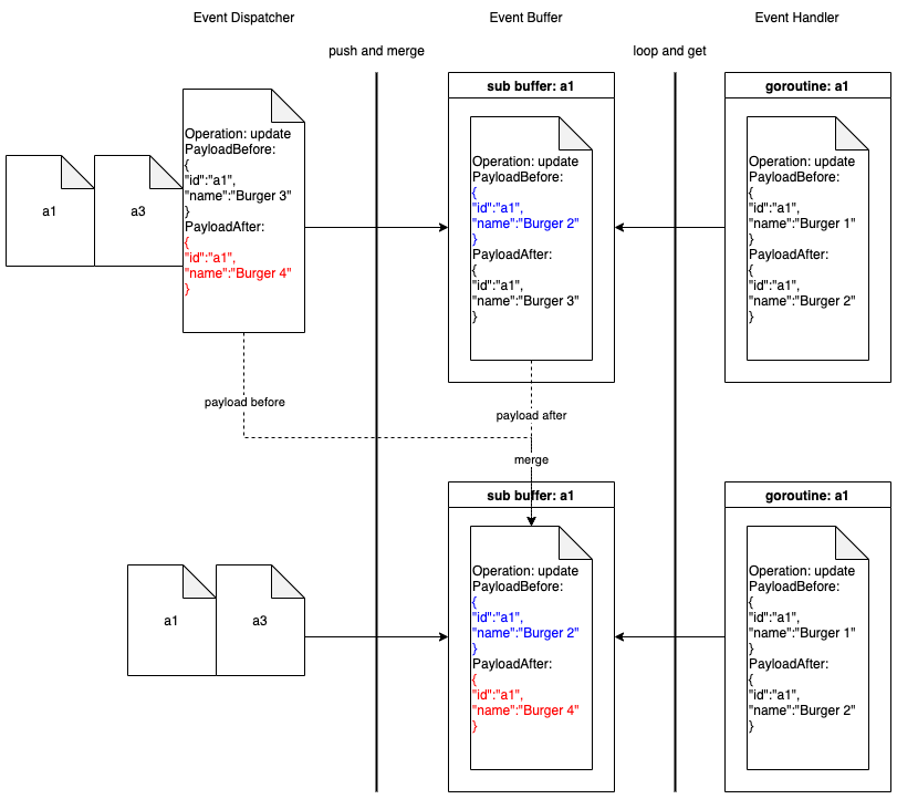
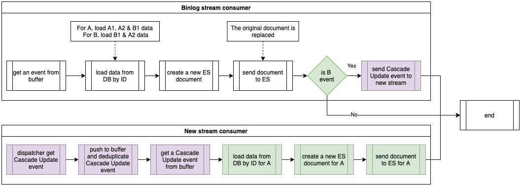
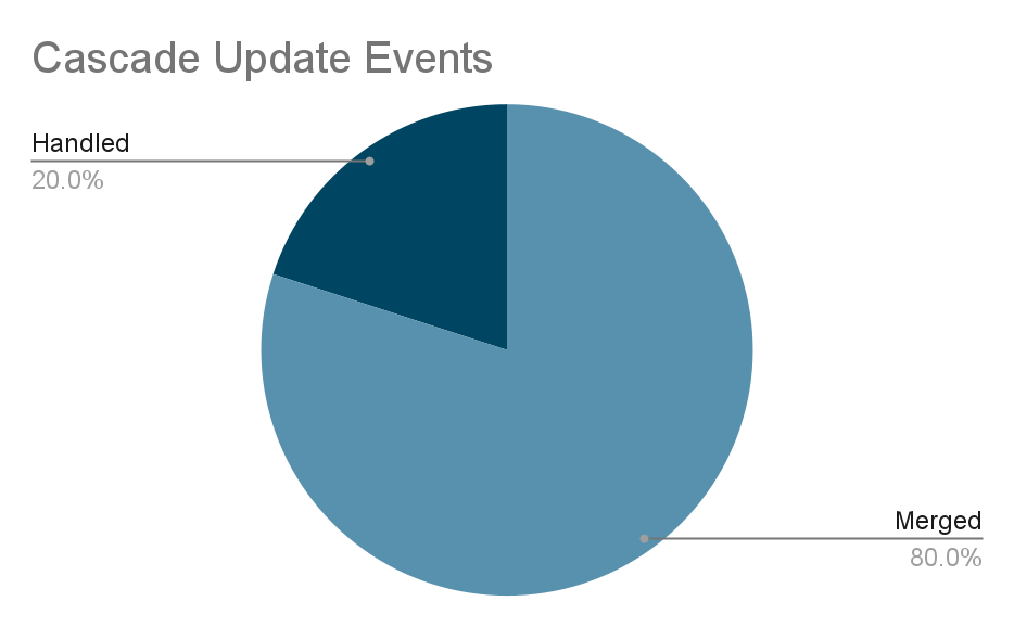
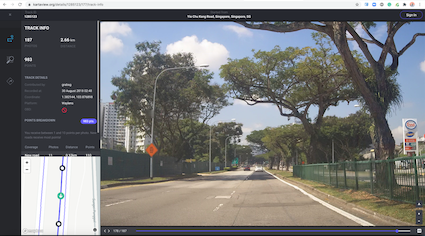
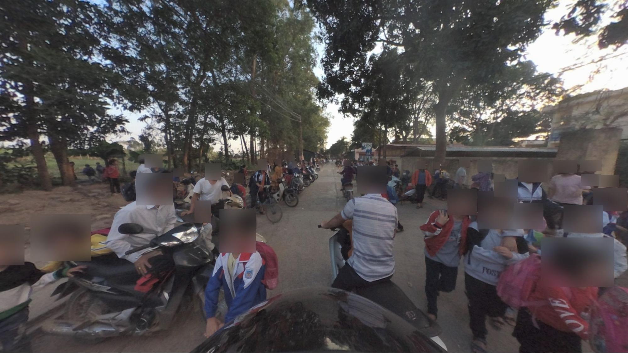
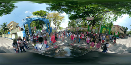
![Figure 4 - Picture’s processing steps [8]](https://engineering.grab.com/img/protecting-personal-data-in-grabs-imagery/figure-4-picture-processing-steps.png)
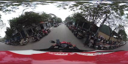
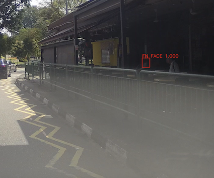
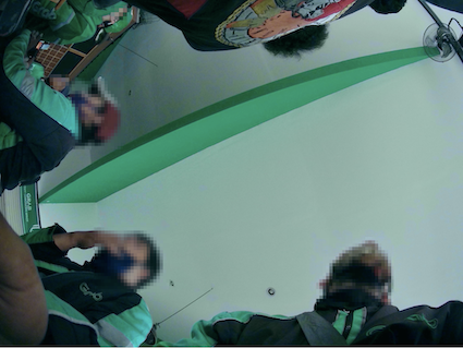




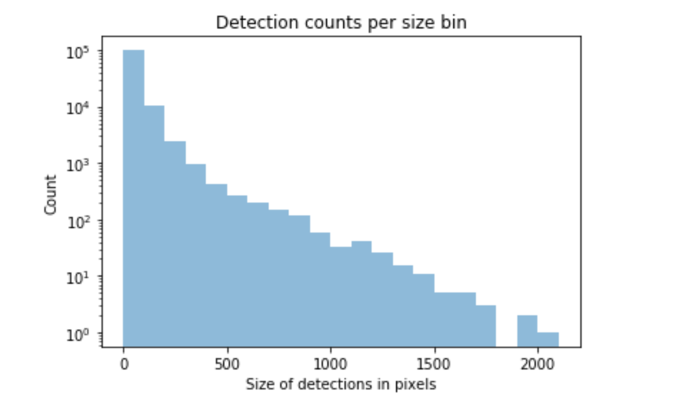
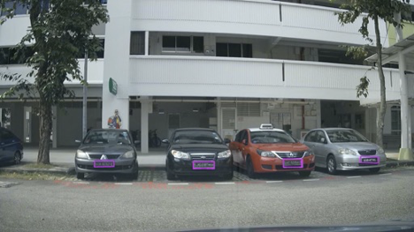
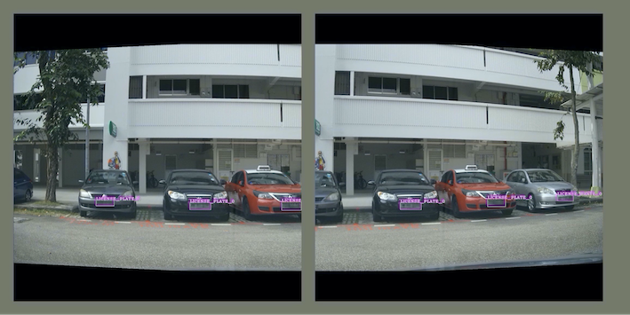
![Figure 7 - Anatomy of one and two-stage object detectors [1]](https://engineering.grab.com/img/protecting-personal-data-in-grabs-imagery/figure-7-anatomy-of-object-detectors.png)