Tag Archives: Platform

Migrating Counter Service storage: Design choices and learnings

Post Syndicated from Grab Tech original https://engineering.grab.com/counter-service-storage-migration

Introduction

Counter Service is used across Grab’s anti-fraud platform to answer time-windowed count questions, such as recent ride requests by a user or failed payment attempts on a card. The service handles tens of thousands of queries per second (QPS) with about a billion requests per day, while maintaining strict requirements around latency and reliability to support real-time fraud rule evaluation.

For most of its life, Counter Service was backed by a wide-column database that served the workload reliably as the service scaled. As part of a broader infrastructure review mandated at an organizational level, our database team evaluated alternatives to this storage that many services relied on, including Counter Service. Based on their assessment, Aerospike emerged as a good fit for our use-case. We also used the migration as an opportunity to decouple storage concerns from business logic, a necessary first step for this migration, and one that would reduce the effort required for future storage changes. As part of the same effort, we revisited the data model and access patterns in detail, which helped us identify and apply several straightforward optimizations.

This post walks through how we did it. What we built on the reader-side to make the migration safe, how we redesigned the writer-side data model around the new backend, and what we ran into during the gradual rollout.

Setting the stage

Counter data is stored in three time granularities: 15-minute, hourly, and daily buckets. A typical read would be along the lines of, “give me the count for key X over the last 90 minutes”, which the service decomposes into the smallest possible set of buckets, one hourly in the middle, a few 15-minute buckets at the edges, fetches them, and sums.

In the original setup, each granularity was stored in a separate table with a composite primary key:

TABLE daily_count (
    key      TEXT,         -- partition key
    day_ts   TIMESTAMP,    -- clustering key
    count    BIGINT,
    PRIMARY KEY (key, day_ts)
);

The clustering column gave us convenient range queries, that is needed for the Counter Service. On the write path, each incoming counter event triggered a read-modify-write, three parallel SELECT across the three tables, an in-memory increment, then a batch write. This produced four network round-trips per event.

As this service is a core part of Grab’s fraud detection ecosystem and handles high query volume, migrating its underlying storage required a careful rollout plan. We had three requirements:

  • Ramp traffic to the new backend gradually and roll back at any point with a config change.
  • Monitor both the original and new storage paths to verify data integrity before switching over.
  • Complete the migration without downtime.

We also wanted the migration machinery to be reusable for future storage changes. The migration is divided into three workstreams, which we’ll walk through below:

  • Preparing the reader service.
  • Identifying the best integration mechanism for the new storage.
  • Updating the writer pipeline.

Reader: Separating the data access layer

The reader is a Rust service. Before any migration work began, the reader’s business logic had tight coupling with the storage layer. Session creation, query building, fan-out orchestration, and the data types those queries returned were all intertwined in a single flat file. The main application state struct (AppState) held a raw database session handle and prepared query references. Every handler, gRPC Remote Procedure Calls (gRPC) or HyperText Transfer Protocol (HTTP), received the bare session as a parameter. Variable names baked the storage technology into the business layer.

This made the storage migration difficult to attempt directly. We couldn’t add a second storage backend without forking the orchestration logic, and we had no way to test the read path in isolation from a real database session. So we did the migration prep in three stages.

Stage 1: Extracting the storage code

The first stage shipped no behavioural change. We deleted the monolithic storage file and split its contents in two:

  • storage/legacy.rs: wrapped session creation, prepared statements, and query execution behind a LegacyStorage struct.
  • batch_read_ops.rs: kept only the orchestration logic: time-range splitting, channel-based fan-out, and aggregation.

AppState started holding an Arc<LegacyStorage> instead of a raw session handle. The PreparedQueries struct lost its statements (those moved inside LegacyStorage). We renamed every storage-specific identifier in business code to generic storage_* names.

The result was a hard fence. After Stage 1, the database driver crate was reachable only from inside the storage module. Nothing in the business logic or handlers imported it any more.

Stage 2: The storage facade

With the seam in place, we introduced the actual abstraction. A new storage/ module with mod.rs, legacy.rs, aerospike.rs, and mock_storage.rs as siblings became the only place driver crates were reachable from.

The idiomatic Rust approach would have been a trait with associated types, but our backend selection is runtime (a config string parsed at startup), and associated types propagate upwards through every consumer. The alternative, trait objects with boxed futures adds a heap allocation per query, which we wanted to avoid at our QPS.

We chose a concrete facade with enum dispatch:

struct Storage {
    legacy:    LegacyStorage,
    aerospike: AerospikeStorage,
    mock:      MockStorage,
    settings:  StorageSettings,
}

execute_queries(backend: BackendType, ...) {
    match backend {
        Legacy    => self.legacy.execute(...),
        Aerospike => self.aerospike.execute(...),
        Mock      => self.mock.execute(...),
    }
}

A match statement at the request boundary, which made it easier to reason about and debug. The facade then routes everything to the original backend without the rest of the code knowing or caring.

Each backend’s execute_queries honours the same contract: take a Vec<QueryCandidate> and a HashMap<BatchIndex, Sender<...>>, and emit (index, value, timestamp, granularity) tuples into those channels. The orchestration layer above doesn’t need to know whether a candidate became a paginated row stream or a single batch read with client-side map filtering, both write into the same channels in the same shape.

On top of the facade we layered three config-driven operating modes that map to the migration phases:

  • Single: one backend serves the request.
  • WithShadow: the primary serves the response; the secondary runs asynchronously in the background for parity comparison.
  • WithSplit: a deterministic percentage of traffic is served by each backend. Used for the live cutover.

The mode and traffic percentages are read from a service config, allowing the reader to move from legacy-only to Aerospike-only without code changes. The transition starts in Single(legacy), then shadow reads are enabled with WithShadow(primary=legacy, secondary=aerospike, pct=X). The shadow percentage is gradually ramped from 5% to 20%, 50%, and finally 100%, while parity is verified through metrics. Optionally, the system can then move into WithSplit(primary=legacy, secondary=aerospike, split=X), where live traffic is gradually shifted from the original backend to Aerospike, for example from 5% to 30%, 70%, and then 100%. Once Aerospike is fully validated and serving all traffic, the reader moves to Single(aerospike).

Stage 3: Shadow comparison and metrics

Each storage call carries metadata like backend, role (primary/secondary/shadow), and mode, attached as tags to every metric. When Aerospike was added, existing dashboards showed per-backend breakdowns without changes.

We placed the mode dispatch at the handler level rather than inside the storage layer to validate the full request path, not only the rows returned by storage. This also lets the response return as soon as the primary completes, while the shadow runs as a fire-and-forget background task.

Writer: redesigning the data model

Since the two systems use different storage engines, it wasn’t clear that a one-to-one port of our original schema would work. We tried three approaches.

Approaches 1 and 2: Row-per-bucket

We first tried mirroring our original row-per-bucket model. Approach 1 used Aerospike’s Secondary Index (SI) to recover range queries; approach 2 skipped SI and computed the exact set of primary keys client-side via BatchGet.

Both hit the same wall: Aerospike’s primary index is 64 bytes per record, kept in memory. At billions of records, index memory becomes the constraint. SI added overhead and operational complexity we didn’t need.

Approach 3: Map-based schema

The third approach was structurally different from the first two and was the most compact of the options. Rather than storing one record per bucket, which kept us in the same cardinality regime, we collapsed all bucket counts for a single counter into one record. The values were stored as a sorted map keyed by bucket timestamp:

Set:           helium_hourly
Primary key:   "{counterKey}"
Bins:
   counts: KEY_ORDERED_MAP({
        1773369000000: 1,
        1773372600000: 3,
        1773376200000: 7,
        ...
   })

The map keys are bucket timestamps in milliseconds. The map values are running counts. One record holds the entire time series for one counter at one granularity.

Reads become straightforward: fetch the record, iterate the map, sum the entries within the requested window. Each Get returns a bounded number of map entries (determined by Time To Live (TTL) and bucket size), and client-side filtering of that many entries is negligible.

Writes use MapIncrementOp, an atomic server-side increment of a value at a given map key, creating the entry on first access. Combined with MapRemoveByKeyRangeOp for pruning stale entries, every write is one atomic operation:

ops = [
    MapIncrementOp(counts, bucketTsMs, delta),
    MapRemoveByKeyRangeOp(counts, 0, cutoffMs),
    PutOp(key_bin, counterKey),
]
client.Operate(policy, key, ops)

For TTL management, we couldn’t use Aerospike’s record-level expiry directly. A single record holds many timestamps, so record-level TTL would either keep everything or drop everything. Instead, we prune stale map entries explicitly on every write using MapRemoveByKeyRangeOp. The record-level TTL stays as a safety net for counters that stop receiving writes.

The two backends produce very different network shapes for the same logical query. The original backend returns many small paginated row streams, one per (key, granularity). The server filters by time range using the clustering column. Aerospike returns one batch response with the entire counts map per key, and the client filters the map to the requested range. The reader’s storage layer hides this difference: both paths emit (index, value, timestamp, granularity) tuples into the same per-index channels, and the orchestrator above sums them the same way.

The third approach performed best in testing. By collapsing many bucket records into a single record per counter, we reduced the total record count by more than an order of magnitude, which also reduced primary index memory. It also produced a smaller on-disk footprint, since the long counter key is stored once per record instead of being repeated across every bucket. The schema was chosen to fit the access pattern, with the index and disk savings following naturally.

The pipeline continues writing to the original backend as the primary, while Aerospike is added as a separate asynchronous shadow write behind a deterministic rollout logic. This lets us ramp Aerospike gradually and eventually cut over to it fully.

Reader: How each backend actually serves a query

The two storage backends sit behind the same execute_queries contract on the reader service, but what they do internally for a single batch read looks very different.
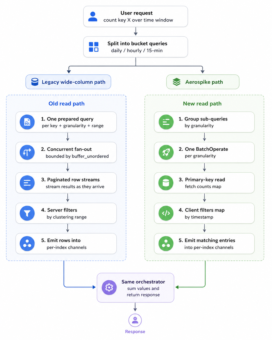
Figure 1. How a single read request flows through each backend.

The reader takes a batch of counter queries and decomposes each into one or more sub-queries per granularity (a 90-minute window for instance, becomes one hourly sub-query and two 15-minute sub-queries). In the original backend, each sub-query becomes its own prepared statement bound with (start_ms, end_ms, key), and the storage layer fires all of them concurrently as a stream of futures with buffer_unordered capping in-flight queries to a tuned bound. Each query returns a paginated row iterator, the server uses the clustering column to filter by time range and rows stream through to per-index channels as they arrive. So a single user request can produce many small queries, each a separate network round-trip to the partition master holding key, with results dribbled back over a paginated stream.

On Aerospike, the storage layer first groups all sub-queries by granularity, then issues one BatchOperate per granularity. Each sub-query becomes a single primary-key read against the appropriate set; the server returns the entire counts map for that key in one record. The client iterates the map and emits only the entries whose timestamps fall inside the requested range. This keeps the code simple, and at our map sizes the overhead is negligible. There’s no streaming, a batch read either succeeds or fails as a unit and there are at most three network round-trips per user request, one per granularity, regardless of how many sub-queries there are.

This reflects the different design philosophies of the two systems. Wide-column stores typically expect client-side fan-out for reads, while Aerospike’s batch API is designed for exactly this multi-key pattern.

A few issues with the Aerospike Rust client also surfaced during rollout, as it was less mature than its Go counterpart. For example, when we started, the officially available Rust client was synchronous, so every batch read had to be bridged through tokio::task::spawn_blocking with some amount of custom plumbing. Once the official async client was released, we removed that layer and saw measurable improvements in both p50 and p99 latency. The other issue was Domain Name System (DNS). The client resolved seed hostnames only during initialization and did not re-resolve them when the cluster topology refreshed. As a result, a full staging cluster replacement, with new IPs behind the same hostnames, left the client stuck on the old IPs until restart. We filed the bug upstream, and a fix shipped in a subsequent release. We also reproduced the scenario locally with a Docker-based end-to-end test and ran additional staging drills to confirm recovery before continuing the rollout.

Experiment with indexing

We run Aerospike in its default storage configuration, Hybrid Memory Architecture (HMA), where the primary index sits in Random-Access Memory (RAM) and the data sits on Solid-State Drive (SSD). The other relevant mode keeps both index and data in Dynamic Random-Access Memory (DRAM), which is more expensive and not something that fits our use-case. Even in HMA, the primary index grows linearly with record count. At our scale, that growth was a foreseeable issue.

To raise the memory ceiling, we tried moving the primary index itself from RAM to local Non-Volatile Memory Express (NVMe) while keeping data on SSD. We expected the extra index latency to be invisible within our overall request budget. In practice, we started seeing p99 spikes that did not track overall QPS. Instead, they followed I/O activity on hot keys. We observed that when many concurrent lookups land on the same record, the in-memory index handles them more prudently compared to a disk backed index. Adding more and better nodes improved things slightly but did not mitigate the issue. Consequently, we reverted back to in-memory index with a memory-optimized instance type.

Overall impact

The migration delivered gains across infrastructure, performance, and data footprint. Most of these improvements trace back to the schema redesign like collapsing rows into maps, rather than the database change itself.

The primary index currently uses about 50 GB of the roughly 100 GB usable memory per node. The same dataset is around 1 TB on disk, compared with around 3 TB on the original setup. This is primarily attributed to our adoption of the map-based schema discussed earlier.

In production, p99 read latency was consistently better than the original setup, with roughly 50% improvement across our read paths. The write path now uses a single atomic increment operation, replacing the read-modify-write pattern we had built previously.

The new setup costs roughly 45–50% less per node compared to our original setup. We also reduced the replication factor from 3 to 2, saving roughly a third of both storage and primary index memory. RF=2 can be awkward in databases that depend on write quorum, but Aerospike’s master-replica model still keeps an authoritative copy available after a single-node loss. That gives us meaningful fault tolerance even at RF=2. The remaining risk, a simultaneous multi-AZ failure, was acceptable for this workload because the writer continues producing increments from the source event stream. Any lost counter data can self-heal as new events arrive.

Conclusion

This migration ultimately came down to aligning the storage design with the workload. These results would not have been achieved by simply swapping one storage system for another. As the service evolved over time, our initial design choices became less optimal, and the migration surfaced opportunities to rethink them. The gains came from focusing on optimization opportunities, redesigning the data model, and cleanly separating storage concerns. Through shadow reads and writes, followed by a gradual rollout, we completed the migration with zero downtime and no data-integrity issues. The result is a system that fits its workload well and a foundation that makes future storage changes safer and easier to attempt.

Join us

Grab is Southeast Asia’s leading superapp, serving over 900 cities across eight countries (Cambodia, Indonesia, Malaysia, Myanmar, the Philippines, Singapore, Thailand, and Vietnam). Through a single platform, millions of users access mobility, delivery, and digital financial services, including ride-hailing, food delivery, payments, lending, and digital banking via GXS Bank and GXBank. Founded in 2012, Grab’s mission is to drive Southeast Asia forward by creating economic empowerment for everyone while delivering sustainable financial performance and positive social impact.

Powered by technology and driven by heart, our mission is to drive Southeast Asia forward by creating economic empowerment for everyone. If this mission speaks to you, join our team today!
Palana (Part 2): Architecting isolation, identity, and auditability for AI agents

Post Syndicated from Grab Tech original https://engineering.grab.com/part-2-palana-architecture

Introduction

In Part 1, we introduced Palana, Grab’s Kubernetes-native secure execution platform for autonomous AI agents. We discussed the underlying need for isolated environments and covered its core design principles: treating isolation as the unit of trust, keeping credentials out of agent hands, and mediating all network access. In this second part, we’ll dive under the hood into Palana’s architecture, look at the agent lifecycle, and share the key lessons we learned from putting this system into production.

Architecture overview

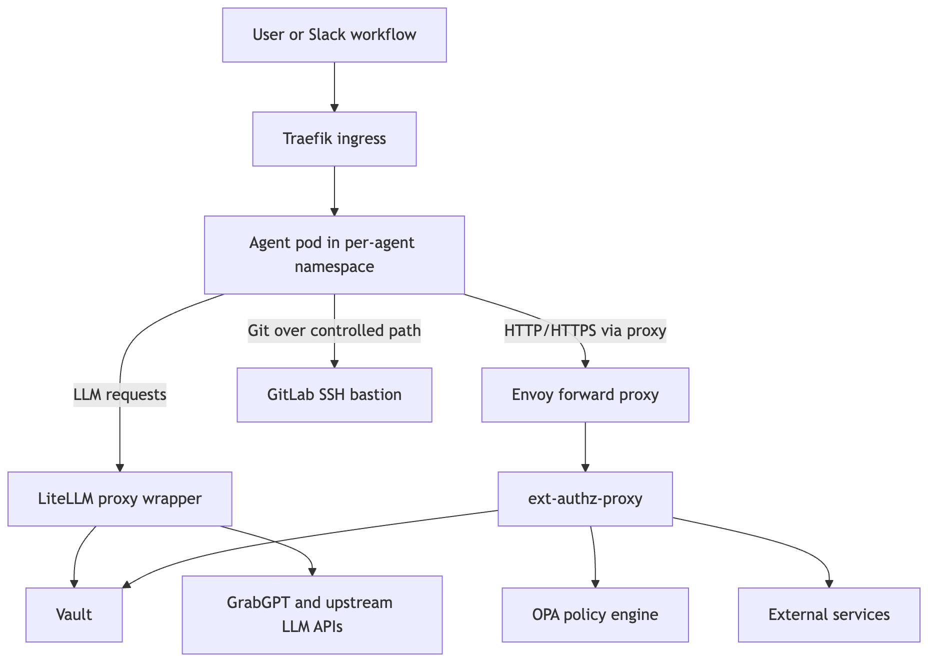
The core request path looks like this:

Figure 1. Palana architecture overview.

The agent pod runs in a namespace owned by one user and one agent. It gets default-deny style network policy, domain name system (DNS), access to required platform services, and a persistent /data volume. Browser traffic enters through Traefik. LLM traffic goes to the LiteLLM wrapper in the gateway namespace. General Hypertext Transfer Protocol (HTTP) and Hypertext Transfer Protocol Secure (HTTPS) egress goes through the proxy namespace. Secrets are read from Vault only by the component authorized to use them.

The operator is responsible for turning a user request into the concrete Kubernetes shape:

  1. The user creates an agent through pcli (Palana command-line interface) or the portal.
  2. Palana writes a UserAgent or Agent custom resource with the raw user identity.
  3. The operator creates the user and agent namespaces, service accounts, role bindings, storage, network policies, and ingress.
  4. The user runs a template or container image.
  5. Admission webhooks inject proxy environment variables and enforce pod-level restrictions.
  6. Logs, policy decisions, and activity signals are emitted to observability systems.

Agent lifecycle

From a user’s perspective, the basic workflow is intentionally small:

./pcli login
./pcli create demo
./pcli secrets add demo GRABGPT_API_KEY token=<token>
./pcli run demo --template claudecodeui

Behind those commands, Palana provisions an isolated execution environment:

  • Namespace: agent-{sanitized-user}-{agent}
  • Service account: bound only to that namespace
  • Storage: an Amazon Elastic File System (EFS)-backed persistent volume claim (PVC) mounted at /data
  • Ingress: an agent-specific hostname protected by Concedo-backed browser auth
  • Egress: forced through platform proxies, except for approved internal platform services
  • Secrets: split between agent-readable and proxy-only Vault paths
  • Policies: proxy egress, network egress, and optional inter-agent peering rules

The same lifecycle is exposed in the portal for users who prefer a browser user interface (UI).

How Palana handles identity

Human authentication uses Concedo OpenID Connect (OIDC). pcli login performs a browser-based authorization code flow with Proof Key for Code Exchange (PKCE) and stores the resulting identity in an isolated kubeconfig. Browser access to agent UIs is protected by OAuth2-Proxy through Traefik forward auth.

The important detail is that Palana keeps the raw user identity, such as an email address, as the authoritative owner on the custom resource. That raw identity is used for Kubernetes role-based access control (RBAC) subject matching. Sanitized forms are used only where Kubernetes object names, labels, namespaces, or Vault paths require safer strings.

This split prevents a common class of identity bugs: the display-safe or path-safe version of a user ID should not accidentally become the authorization subject.

In the future, we will integrate Palana via SPIFFE (Secure Production Identity Framework for Everyone) and SPIRE (SPIFFE Runtime Environment) with the rest of our service mesh, to provide an agentic identity — a combination of user and agent instance id — that can then be controlled as a subset of a user’s capabilities. This gives us a first step into “agents on behalf of users” with cut-down permissions while the wider industry firms up the approaches via Open Authorization (OAuth) and other controls.

How Palana handles secrets

Palana’s Vault layout is designed around least privilege:

kv/agents/{user}/{agent}/{secret}
kv/proxy-secrets/{user}/{agent}/{secret}

The first path is for secrets the agent is allowed to read through its per-agent Vault role. The second path is for credentials the agent can use only through the proxy. For each proxy-only secret, Palana can create an agent-visible placeholder value. The placeholder is inert unless the request goes through the approved proxy path.

This gives teams a practical migration path. Existing clients can often be configured with a token-looking value, while Palana keeps the real token out of the runtime.

How Palana handles LLM access

LLM calls go through litellm-proxy-wrapper, which sits in front of LiteLLM and GrabGPT. The wrapper derives agent identity from Kubernetes context rather than trusting client-provided headers. It then looks up the per-agent GrabGPT credential in Vault and forwards the request to the correct upstream route.

The agent config uses internal base URLs such as:

http://litellm-proxy.gateway:4000/aws/v1
http://litellm-proxy.gateway:4000/unified/v1

That design gives us three useful properties:

  • Agents do not need raw upstream LLM credentials.
  • LLM traffic is attributable to a specific agent.
  • Provider routing and credential handling can evolve centrally.

How Palana handles network access

Network control is split into two layers.

At Layer 3 and Layer 4, Kubernetes NetworkPolicy and Cilium enforce which pods can talk to which namespaces, services, and classless inter-domain routing (CIDR) blocks. Agent namespaces are locked down to the platform paths they need: DNS, Vault, the egress proxy, the LLM gateway, and the Kubernetes application programming interface (API) patterns the platform explicitly supports.

At Layer 7, the proxy policy controls HTTP and HTTPS destinations by host, method, and agent identity. Open Policy Agent (OPA) evaluates per-agent policy. The proxy logs allow and deny decisions in structured form.

This split is deliberate. NetworkPolicy is good at containment. The proxy is good at application-aware decisions and audit. This allows us to be very expressive in the restrictions we place on our agents — by default, they get nothing; if they should have access to an internal service they get only that service, and cannot be used as an entry point to the wider internal environment.

Observability and operations

Palana treats observability as part of the safety model, not a nice-to-have. The platform emits structured logs for proxy decisions, Git activity, LLM requests, agent lifecycle, and idle-shutdown decisions. Operators can query activity by namespace, user, host, decision, or component.

One example is idle shutdown. Long-running agents are useful, but idle workloads consume cluster resources and expand the surface area that platform teams must monitor. Palana’s reaper records the most recent observable activity for each UserAgent. It combines signals from gateway/proxy logs, Git activity, Slack-routed agent messages, and Prometheus network activity. After a configurable idle threshold, it can warn the user and stop the workload while preserving /data, RBAC, namespace, and Vault state.

This is a good example of the platform philosophy: stop the compute, keep the state, and make resumption easy.

In addition, as we move into agentic operations, we use the many signals generated by Palana itself to aid our agents. For example, we have an agent that can monitor user workloads and provide advice and assistance if it spots issues — say, an agent is consistently out of memory (OOM), the ops agent can see that and message the user with instructions on how to increase the allocated memory. We don’t need to special-case every possible issue; instead we have agents that understand Palana logs and are able to communicate with the users themselves.

What we learned

Agent platforms need security controls at the platform layer

Prompt-level guardrails and model policies are useful, but they are not enough. Agents call tools, tools call services, and services use credentials. Palana puts controls where the action crosses a trust boundary: identity, egress, secrets, ingress, Git, and Kubernetes API access.

The user experience matters as much as the control

If the secure path requires every team to learn Terraform, Vault policy syntax, Kubernetes RBAC, and proxy configuration before they can try an agent, teams will work around it. Palana uses pcli, templates, and the portal to make the safe path the easy path.

Separating “can read a credential” from “can cause a credentialed request” is powerful

Proxy-only secrets are one of the highest-leverage design choices. They let agents perform authenticated work without turning the agent filesystem, logs, process environment, or prompt context into a credential store.

A namespace boundary is simple, but it compounds

Per-agent namespaces give us a consistent place to apply RBAC, storage, network policy, logging labels, resource quotas, and lifecycle controls. The pattern is easy to reason about during incidents: identify the namespace, identify the owner, inspect the policy, and isolate if needed.

Long-running agents need lifecycle management

Once agents persist for days or weeks, “run a container” becomes an incomplete product. Users need resume semantics. Operators need idle cleanup. Security teams need audit history. Platform teams need a way to rotate credentials, update images, and stop workloads externally.

What’s next

Palana is increasingly becoming a substrate for larger autonomous systems rather than only a place to run individual agents. Emerging patterns include:

  • Supervisor systems that route work to a pool of scoped agents.
  • Slack-native agents that wake up, handle a task, and scale back down.
  • Remote development environments backed by persistent cloud state.
  • Agent swarms where each worker has a separate namespace and credential scope.
  • Operational agents that investigate platform health and propose or apply small fixes under policy.
  • Security experiments around supply chain monitoring, token rotation, transport layer security (TLS) inspection, and automated isolation.

The north star is not “let every agent do anything”. It is to make useful autonomy boring to operate: attributable, inspectable, revocable, and recoverable.

Conclusion

AI agents are most valuable when they can act in real environments. That is also when they become risky. Palana gives Grab a way to keep both sides of that tradeoff in view: teams can move quickly with self-service agent environments, while the platform keeps isolation, identity, secrets, network access, and auditability as defaults.

We expect the underlying tools and models to keep changing. The platform primitives are more durable. Agents will vary, but they will still need a place to run, a way to authenticate, a boundary around their actions, and a record of what happened.

That is the role Palana is designed to play.

Join us

Grab is Southeast Asia’s leading superapp, serving over 900 cities across eight countries (Cambodia, Indonesia, Malaysia, Myanmar, the Philippines, Singapore, Thailand, and Vietnam). Through a single platform, millions of users access mobility, delivery, and digital financial services, including ride-hailing, food delivery, payments, lending, and digital banking via GXS Bank and GXBank. Founded in 2012, Grab’s mission is to drive Southeast Asia forward by creating economic empowerment for everyone while delivering sustainable financial performance and positive social impact.

Powered by technology and driven by heart, our mission is to drive Southeast Asia forward by creating economic empowerment for everyone. If this mission speaks to you, join our team today!
Palana (Part 1): Why Grab built a secure platform for autonomous AI Agents

Post Syndicated from Grab Tech original https://engineering.grab.com/palana-part-1-secure-platform-for-ai-agents

Abstract

Artificial intelligence (AI) agents are moving from experiments into everyday engineering workflows. They can read code, call application programming interfaces (APIs), run tests, create merge requests, answer Slack messages, and keep long-running state. That makes them useful, but it also changes the risk model – especially as agents get more autonomous in their use of tools. An agent with network access, credentials, tools, and memory is no longer just a chat interface. It is a workload that can act.

The more capability we give to the agents, the more valuable they get – but they also get riskier, and maintaining controls and oversight gets more challenging. We need isolated environments, with clear intentional capabilities added rather than just inheriting “everything on your laptop”.

Palana is Grab’s Kubernetes-native platform for running those workloads safely. It gives each agent an isolated namespace, persistent storage, controlled ingress, proxy-mediated egress, Vault-backed credential injection, large language model (LLM) routing, Git access controls, structured audit logs, and emergency kill switches. It is currently used to run hundreds of agents, including remote development environments, Slack automation, OpenClaw workers, Hermes agents, and other long-running internal systems.

In this post, we share why we built Palana, what it does, and how its architecture lets teams experiment with autonomous agents without giving up control over identity, secrets, network access, and operational visibility.

Introduction

The first wave of AI coding tools lived close to the user: an integrated development environment (IDE) plugin, a chat window, or a command-line assistant running on a developer’s laptop. That model is familiar and easy to adopt, but it has limits. Long-running agents need persistent state. Team workflows need shared access through Slack or web user interfaces (UIs). Security teams need to inspect what an agent is doing, and apply highly granular controls over what an agent can do. Platform teams need a way to stop, resume, update, and audit the workload.

As usage grew, we started seeing the same question in different forms:

How do we let agents do useful work inside the company without treating every new agent as a bespoke infrastructure project?

The answer was not simply to “run agents in containers”. Containers help package the runtime, but they do not answer the harder platform questions:

  • Which user does this agent act on behalf of?
  • What credentials can it use?
  • Can it see another user’s state?
  • Can it connect directly to the internet?
  • How do we inspect LLM, Git, and Hypertext Transfer Protocol (HTTP) activity after something goes wrong?
  • How do we stop an agent quickly without trusting the agent to cooperate?
  • How do we give teams a self-service experience without handing them cluster-admin access?

Palana is our answer to those questions.

What Palana is

Palana, an in-house proprietary system built by the CyberSecurity team at Grab, is a secure execution substrate for autonomous and semi-autonomous agents. The name comes from a Sanskrit root associated with protection, maintenance, and care. That maps well to the platform’s purpose: Palana is not trying to be the agent’s brain. It is the environment that contains, observes, and sustains the agent while it works.

At a high level, Palana provides:

  • A Kubernetes namespace per agent, with role-based access control (RBAC), resource quotas, network policy, and storage scoped to that agent.
  • A command-line and portal experience for creating, running, stopping, configuring, and inspecting agents.
  • Persistent /data storage so long-running agents can preserve memory, caches, repositories, and session state across restarts.
  • Browser and shell access for interactive workloads such as Claude Code UI, OpenCode, IDEs, ttyd, or Secure Shell (SSH)-backed development flows.
  • LLM access through a LiteLLM wrapper that injects per-agent GrabGPT credentials from Vault.
  • HTTP and HTTPS egress through an Envoy and ext-authz proxy path, with Open Policy Agent (OPA) policy checks and structured request logs.
  • Proxy-only secrets, where agents can reference placeholder tokens but cannot read the underlying credentials directly.
  • Git access through a bastion path so repository operations are attributable and policy-controlled.
  • Kill switches and idle shutdown so the control plane can isolate or stop workloads from outside the agent process.

This combination lets Palana support several categories of work:

  • Secure OpenClaw and agent-framework testing.
  • Cloud development environments accessible from a browser or SSH client.
  • Fast prototyping and testing for agentic workloads in a secure environment.
  • Slack-connected agents such as cts-aergia and Claude-to-Slack workflows.
  • Long-running task agents such as Hermes, Matlock, Butler, and custom team automations.
  • Higher-order systems where agentic supervisors launch or route work to scoped agents.

Why we built it

The immediate need came from security research. We wanted a place to run and investigate OpenClaw and related agent frameworks without exposing the broader internal network or placing raw credentials inside the agent runtime. That use case forced us to design for containment from the beginning.

The broader need quickly became developer productivity. Once the basic primitives existed, Palana became useful for remote coding, Slack automation, internal assistants, long-lived experiments, and agentic operational workflows. Grabbers wanted agents that could keep context over days or weeks, run from corporate infrastructure, access approved internal services, and survive laptop sleep, local dependency drift, or network changes.

The security and productivity goals reinforce each other. If the safe path is self-service and ergonomic, teams are more likely to use it. If the productive path is observable and policy-controlled by default, and the appropriate security is baked into the system automatically, platform teams do not have to retrofit controls after adoption.

Design principles

Palana’s architecture follows a few principles that shaped most of the implementation.

Isolation is the unit of trust

Each agent gets its own namespace, service account, storage, network policy, and Vault scope. Agents should not see each other’s pods, secrets, or filesystem state by default. Inter-agent communication is possible, but it goes through explicit peering rules rather than ambient pod-to-pod reachability.

This means the platform does not have to assume every agent framework has perfect multi-tenant isolation internally. A framework designed as a single-user assistant can still be hosted safely by giving each user or worker its own Palana boundary.

Credentials are never given to the agent

Traditional application hosting often gives credentials to the workload as environment variables or mounted files. That is risky for agent workloads because the agent may execute tools, run untrusted code, summarize files, install packages, or expose a web UI.

Palana separates two kinds of secrets:

  • Agent-readable secrets live under the agent’s own Vault path and are available only to that agent’s service account.
  • Proxy-only secrets are stored under a separate Vault path and are read by the proxy layer, not by the agent.

For proxy-only secrets, the agent sees a placeholder such as TOKEN_GITHUB_PAT or TOKEN_GRABGPT_API_KEY. When an outbound request travels through the proxy path, the proxy replaces the placeholder header with the real credential from Vault. The remote service receives a valid token, but the agent process never stores the token in its own environment or config.

This pattern is especially important for LLMs, source control, API integrations, and browser-like tools where prompt injection or dependency compromise could otherwise expose long-lived credentials.

Egress is a control point

Agents can be useful only if they can call tools and services. Instead of forbidding network access, Palana makes network access observable and policy-mediated.

Agent pods receive proxy configuration automatically. External HTTP and HTTPS traffic flows through Envoy. Envoy asks ext-authz-proxy to identify the calling pod, evaluate policy with OPA, log the request, and optionally inject credentials. HTTPS traffic can be terminated by the proxy’s man-in-the-middle (MITM) listener for header inspection and replacement, with the generated certificate authority (CA) distributed to agent pods.

This gives the platform a place to answer questions that normal Kubernetes networking cannot answer alone:

  • Which agent made this request?
  • Which user owns that agent?
  • Which host and method were requested?
  • Was the request allowed or denied?
  • Which placeholder credentials were replaced?
  • Did the request go to an internal service, an LLM gateway, GitLab, or the public internet?

The control plane must stay outside the agent

Palana assumes an agent might become confused, compromised, or uncooperative. Operational controls therefore live outside the agent process. The operator reconciles namespaces and policies. The proxy controls egress. The portal and pcli (Palana command-line interface) manage lifecycle. The kill switch is enforced with network policy. Idle shutdown is handled by a separate reaper CronJob.

That separation matters. A kill switch that asks the agent to stop is a feature. A kill switch that removes the agent’s network path is a safety control.

Use Kubernetes primitives where they fit

Palana is intentionally Kubernetes-native. Agents are represented by custom resources. The operator reconciles namespaces, RBAC, storage, services, ingress, and network policies. Users can interact through pcli or the portal, while platform engineers can still inspect the underlying Kubernetes objects when debugging.

This gives us a layered experience: simple workflows for users, direct primitives for advanced operators, and infrastructure-as-code for the deployed platform.

Conclusion

By centering the design around isolation, controlled egress, and proxy-mediated secrets, Palana provides a secure foundation for AI agents to operate within Grab. In Part 2, we will dive deeper into the under-the-hood architecture of Palana, exploring how it orchestrates agent lifecycles, handles LLM routing, and maintains operational visibility.

Join us

Grab is Southeast Asia’s leading superapp, serving over 900 cities across eight countries (Cambodia, Indonesia, Malaysia, Myanmar, the Philippines, Singapore, Thailand, and Vietnam). Through a single platform, millions of users access mobility, delivery, and digital financial services, including ride-hailing, food delivery, payments, lending, and digital banking via GXS Bank and GXBank. Founded in 2012, Grab’s mission is to drive Southeast Asia forward by creating economic empowerment for everyone while delivering sustainable financial performance and positive social impact.

Powered by technology and driven by heart, our mission is to drive Southeast Asia forward by creating economic empowerment for everyone. If this mission speaks to you, join our team today!
Improving Hugo stability and addressing oncall challenges through automation

Post Syndicated from Grab Tech original https://engineering.grab.com/improving-hugo-stability

Introduction

Hugo plays a pivotal role in enabling data ingestion for Grab’s data lake, managing over 4,000 pipelines onboarded by users. The stability of Hugo pipelines is contingent upon the health of both the data sources and various Hugo components. Given the complexity of this system, pipeline failures occasionally occur, necessitating user intervention when retry mechanisms prove insufficient. These incidents present challenges such as:

  • Limited user visibility into pipeline issues.
  • Uncertainty about resolution steps due to extensive documentation.
  • An overwhelmed Hugo on-call team dealing with ad-hoc requests and growing infrastructure dependencies.
  • Raised Data Production Issues (DPIs) lacking clear Root Cause Analysis (RCA), hindering effective management.

Such challenges ultimately increase data downtime due to prolonged issue triage and resolution times.

To address these problems, we conducted a thorough analysis of failure modes and the efforts required to resolve them. Based on our findings, we propose a comprehensive automation solution.

This blog outlines the architecture and implementation of our proposed solution, consisting of modules like Signal, Diagnosis, RCA Table, Auto-resolution, Data Health API, and Data Health WorkBench, each with a specific function to enhance Hugo’s monitoring, diagnosis, and resolution capabilities.

The blog further details the impact of these automated features, such as enhanced data visibility, reduced on-call workload, and concludes with our next steps, which focus on advancing auto-resolution strategies, enriching the Data Health Workbench, and broadening diagnostics to include more infrastructure components, like Flink, for comprehensive coverage.

Architecture details

We designed the solution based on these principles:

  1. Identify different failure modes based on past issues and analysis from first principles.
  2. Analyse temporal relationships of pipeline execution steps to diagnose issues to failure modes.
  3. Focus on auto-resolution, and add additional features to cover gaps which can’t be immediately addressed by auto-resolution or diagnosis.

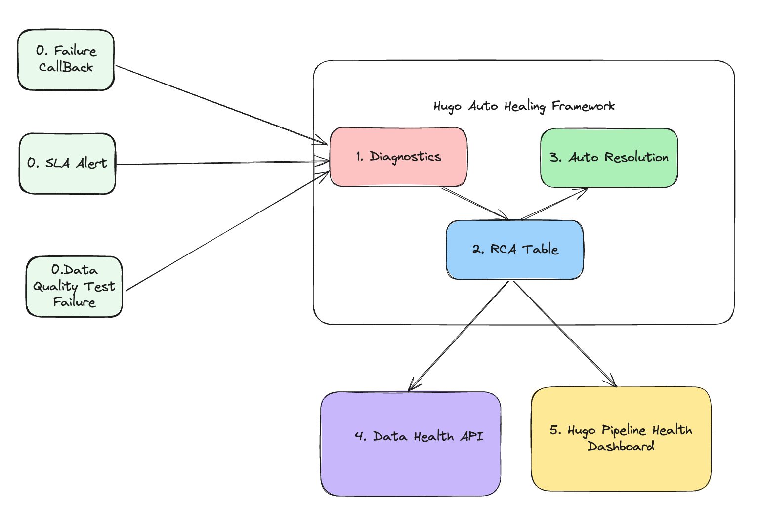
The following diagram shows the solution we proposed.

Figure 1. Architecture

The architecture consists of five core modules, each with a specific function:

  1. Signal module: This module is responsible for collecting signals. It gathers three different types of signals that collectively define the health status of the data lake table. The signals include:
    • Failure callback signal: This indicates whether the pipeline runs involving this data lake table are successful or not.
    • SLA alert signal: This indicates whether the pipeline execution involving this data lake table meets the Service Level Agreement (SLA). For an hourly batch job, the expectation is to complete within one hour.
    • Data quality test failure signal: This represents various types of completeness checks to ensure that data lake tables are consistent with the source tables based on their pipeline strategies.
  2. Diagnosis module: This is the core module responsible for diagnosing the root cause of 3 types of failures collected in the Signal module. It determines:
    • The root cause of the failure.
    • The assignee responsible for fixing the error.
    • The auto-resolution method to fix the issue.
    • Manual resolution steps if the auto-resolution fails.
  3. RCA table: This module stores the following information:
    • Signals
    • Assignee information
    • Diagnosis results
    • Auto-resolution methods
    • Manual resolution steps
  4. Auto-resolution module: This module executes the auto-resolution methods to resolve issues automatically.
  5. Data health API: This module provides API access to other platforms. External platforms or pipelines that rely on Hugo onboarded tables can subscribe to the health status and investigate the root cause when a table is deemed unhealthy.
  6. Hugo pipeline health dashboard: A centralised dashboard for Hugo users to visualise the health status of tables, auto resolution status, and manual fix button.

By leveraging these modules, the architecture ensures robust monitoring, diagnosis, and resolution of issues, leading to improved data health and operational efficiency.

Implementation

Signal module

There are two methods for generating these three signals. The failure signal is generated through an airflow callback, while the SLA miss and data completeness test signals are produced by Genchi. Genchi is a data quality observability platform at Grab that performs data quality checks and acts as a crucial enabler for the enforcement of data contracts.

Diagnosis module

As soon as an alert is created, the diagnosis begins. To avoid lengthy diagnosis times, Hugo has developed an innovative approach that eliminates the requirement for parsing extensive logs, such as Spark executor logs or Airflow logs. Instead, it gathers signals transmitted by the computation engine or Grab’s internal platforms.

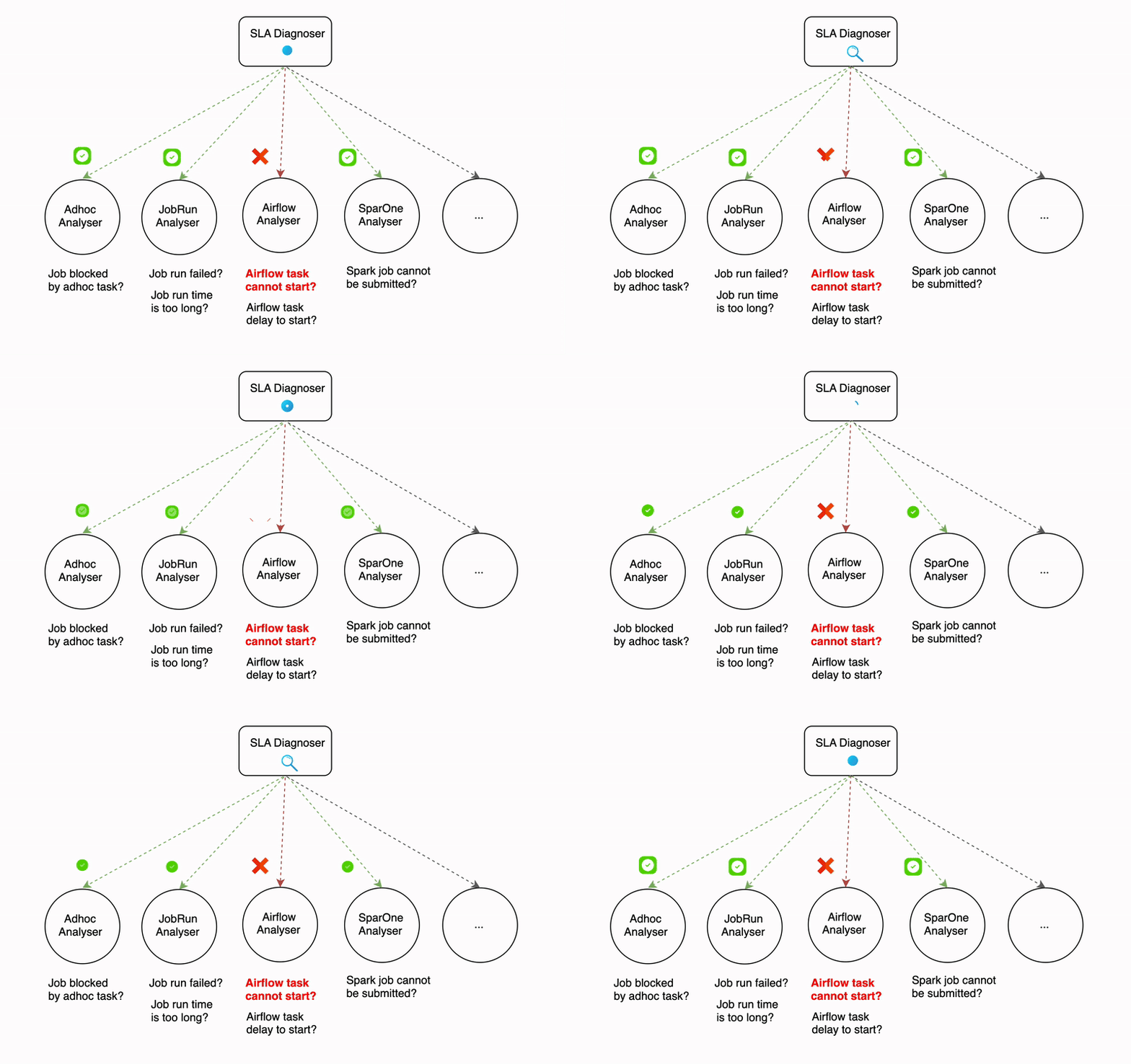
The diagnosis process can be time-consuming, even with efforts to reduce the time it takes. For example, the SLA diagnoser uses multiple analysers that run sequentially, and some of these analysers (like the Airflow analyser) make API calls that can take a significant amount of time. The more analysers that are involved in the diagnosis process, the longer it can take.

Figure 2. Diagnosis process

Parallelism in diagnosis serves as a solution to lower the overall latency when there is a surge in error traffic. The degree of parallelism differs based on the type of signal. For example, the failure signal diagnosis can be executed in thousands of processes at once, while for SLA miss and data quality test failures signals, the parallelism is determined by the number of partitions in the Kafka topic since these signals are received from Kafka.

Auto-resolution module

Auto-resolution is a flexible framework that enables the implementation of custom handlers for various types of failures. One of the common handlers employs a retry mechanism with backoff for transient errors. For instance, if Hugo receives a failure callback indicating that the root cause is a database replica lag, it would wait for an hour before re-triggering the job. This auto-resolution process runs asynchronously with the diagnosis process.

Data health API

The data health information includes a unique identifier, current status, error details, and the time of the last health check, providing a comprehensive snapshot of the dataset’s health.

Hugo converts the detailed information available in its internal data health API to the data health API specification format to be consumed by Kinabalu, our internal system designed to automate and streamline incident management processes by integrating with multiple systems such as Slack, Jira, Splunk on-call, and Datadog.

Hugo pipeline health dashboard

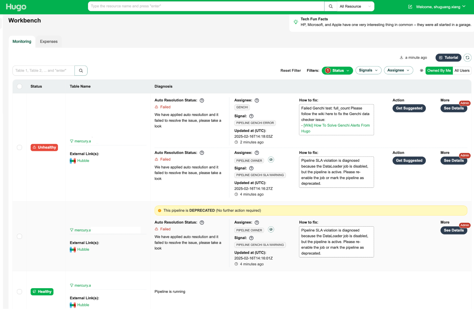
The Data Health Workbench is a centralised dashboard for Hugo users to visualise the health status of tables, auto-resolution status, and manual fix buttons. It provides a comprehensive view of data health and facilitates efficient issue resolution.

The key features are as follows:

  1. Health status visualisation: Displays the current health status of tables, making it easy to identify unhealthy tables.
  2. Assignee information: Indicates the assignee responsible for fixing the issue, ensuring clear accountability.
  3. How-to-fix guide: Provides step-by-step instructions on how to resolve the issue, empowering users to take immediate action.
  4. Action: Offers an action button to initiate the resolution process with a single click, streamlining issue resolution.
  5. Admin feature with detailed diagnosis information: Provides admins supplementary information, including the reasoning behind the root cause identification and assignee determination, which allows for a deeper understanding of the root cause of issues.

By leveraging the Data Health Workbench, Hugo users can efficiently monitor and manage data health, ensuring data integrity and operational efficiency.

Figure 3. Data Health Workbench

Impact

The implementation of Hugo’s auto-healing and diagnosis features has resulted in significant improvements in stability and operational efficiency for our data pipelines. Here are some key outcomes:

  • Enhanced data visibility: We’ve improved the visibility into the health of datasets, allowing for quick identification of issues and more informed decision-making.
  • Timely resolution of data issues: With automated diagnostic and resolution processes, we ensure that data issues are addressed promptly, minimising data downtime and enhancing overall data availability.
  • Reduced on-call workload: By automating many of the common failure resolutions, the workload on Hugo on-call teams has been significantly reduced. This allows teams to focus on more complex and impactful tasks.
  • Scalable solution for managing complexity: The auto-resolution framework is well-equipped to handle the increasing complexity of data infrastructure, offering scalable solutions for transient errors through custom handlers and retry mechanisms.
  • Improved data contract management: By providing detailed pipeline health information via the Data Health API, we enable precise and accurate DPIs, complete with root cause analysis and assignee information, enhancing the management and resolution of data contract breaches.
  • Valuable reference for other platforms: The insights and methodologies developed through this initiative provide a valuable reference for other platform teams at Grab looking to implement similar automation and diagnostic capabilities.
  • Support for Grab’s success: These enhancements support Grabbers by ensuring easy access to the datasets they need and contribute to the overall success of Grab through reliable data availability.

Next steps

Our next steps involve advancing auto-resolution strategies by focusing on complex solutions like pipeline runtime optimisation to boost efficiency and minimise processing delays. We will enrich the Data Health Workbench with detailed information, enabling users to visualise and understand pipeline health more effectively and make informed corrective actions. Additionally, we plan to broaden our diagnosis capabilities by integrating more infrastructure components, such as Flink health information, to ensure a comprehensive and holistic monitoring approach for all engines within Hugo.

Join us

Grab is a leading superapp in Southeast Asia, operating across the deliveries, mobility and digital financial services sectors. Serving over 800 cities in eight Southeast Asian countries, Grab enables millions of people everyday to order food or groceries, send packages, hail a ride or taxi, pay for online purchases or access services such as lending and insurance, all through a single app. Grab was founded in 2012 with the mission to drive Southeast Asia forward by creating economic empowerment for everyone. Grab strives to serve a triple bottom line – we aim to simultaneously deliver financial performance for our shareholders and have a positive social impact, which includes economic empowerment for millions of people in the region, while mitigating our environmental footprint.

Powered by technology and driven by heart, our mission is to drive Southeast Asia forward by creating economic empowerment for everyone. If this mission speaks to you, join our team today!
How Cloudflare is powering the next generation of platforms with Workers

Post Syndicated from Nathan Disidore original http://blog.cloudflare.com/powering-platforms-on-workers/

How Cloudflare is powering the next generation of platforms with Workers

How Cloudflare is powering the next generation of platforms with Workers

We launched Workers for Platforms, our Workers offering for SaaS businesses, almost exactly one year ago to the date! We’ve seen a wide array of customers using Workers for Platforms – from e-commerce to CMS, low-code/no-code platforms and also a new wave of AI businesses running tailored inference models for their end customers!

Let’s take a look back and recap why we built Workers for Platforms, show you some of the most interesting problems our customers have been solving and share new features that are now available!

What is Workers for Platforms?

SaaS businesses are all too familiar with the never ending need to keep up with their users' feature requests. Thinking back, the introduction of Workers at Cloudflare was to solve this very pain point. Workers gave our customers the power to program our network to meet their specific requirements!

Need to implement complex load balancing across many origins? Write a Worker. Want a custom set of WAF rules for each region your business operates in? Go crazy, write a Worker.

We heard the same themes coming up with our customers – which is why we partnered with early customers to build Workers for Platforms. We worked with the Shopify Oxygen team early on in their journey to create a built-in hosting platform for Hydrogen, their Remix-based eCommerce framework. Shopify’s Hydrogen/Oxygen combination gives their merchants the flexibility to build out personalized shopping for buyers. It’s an experience that storefront developers can make their own, and it’s powered by Cloudflare Workers behind the scenes. For more details, check out Shopify’s “How we Built Oxygen” blog post.

Oxygen is Shopify's built-in hosting platform for Hydrogen storefronts, designed to provide users with a seamless experience in deploying and managing their ecommerce sites. Our integration with Workers for Platforms has been instrumental to our success in providing fast, globally-available, and secure storefronts for our merchants. The flexibility of Cloudflare's platform has allowed us to build delightful merchant experiences that integrate effortlessly with the best that the Shopify ecosystem has to offer.
Lance Lafontaine, Senior Developer Shopify Oxygen

Another customer that we’ve been working very closely with is Grafbase. Grafbase started out on the Cloudflare for Startups program, building their company from the ground up on Workers. Grafbase gives their customers the ability to deploy serverless GraphQL backends instantly. On top of that, their developers can build custom GraphQL resolvers to program their own business logic right at the edge. Using Workers and Workers for Platforms means that Grafbase can focus their team on building Grafbase, rather than having to focus on building and architecting at the infrastructure layer.

Our mission at Grafbase is to enable developers to deploy globally fast GraphQL APIs without worrying about complex infrastructure. We provide a unified data layer at the edge that accelerates development by providing a single endpoint for all your data sources. We needed a way to deploy serverless GraphQL gateways for our customers with fast performance globally without cold starts. We experimented with container-based workloads and FaaS solutions, but turned our attention to WebAssembly (Wasm) in order to achieve our performance targets. We chose Rust to build the Grafbase platform for its performance, type system, and its Wasm tooling. Cloudflare Workers was a natural fit for us given our decision to go with Wasm. On top of using Workers to build our platform, we also wanted to give customers the control and flexibility to deploy their own logic. Workers for Platforms gave us the ability to deploy customer code written in JavaScript/TypeScript or Wasm straight to the edge.
Fredrik Björk, Founder & CEO at Grafbase

Over the past year, it’s been incredible seeing the velocity that building on Workers allows companies both big and small to move at.

New building blocks

Workers for Platforms uses Dynamic Dispatch to give our customers, like Shopify and Grafbase, the ability to run their own Worker before user code that’s written by Shopify and Grafbase’s developers is executed. With Dynamic Dispatch, Workers for Platforms customers (referred to as platform customers) can authenticate requests, add context to a request or run any custom code before their developer’s Workers (referred to as user Workers) are called.

This is a key building block for Workers for Platforms, but we’ve also heard requests for even more levels of visibility and control from our platform customers. Delivering on this theme, we’re releasing three new highly requested features:

Outbound Workers

Dynamic Dispatch gives platforms visibility into all incoming requests to their user’s Workers, but customers have also asked for visibility into all outgoing requests from their user’s Workers in order to do things like:

  • Log all subrequests in order to identify malicious hosts or usage patterns
  • Create allow or block lists for hostnames requested by user Workers
  • Configure authentication to your APIs behind the scenes (without end developers needing to set credentials)

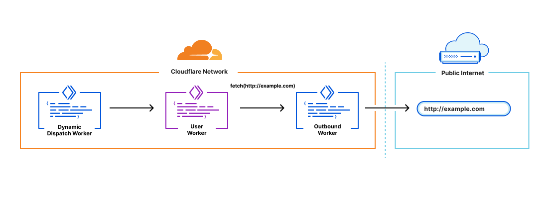
Outbound Workers sit between user Workers and fetch() requests out to the Internet. User Workers will trigger a FetchEvent on the Outbound Worker and from there platform customers have full visibility over the request before it’s sent out.

How Cloudflare is powering the next generation of platforms with Workers

It’s also important to have context in the Outbound Worker to answer questions like “which user Worker is this request coming from?”. You can declare variables to pass through to the Outbound Worker in the dispatch namespaces binding:

[[dispatch_namespaces]]
binding = "dispatcher"
namespace = "<NAMESPACE_NAME>"
outbound = {service = "<SERVICE_NAME>", parameters = [customer_name,url]}

From there, the variables declared in the binding can be accessed in the Outbound Worker through env. <VAR_NAME>.

Custom Limits

Workers are really powerful, but, as a platform, you may want guardrails around their capabilities to shape your pricing and packaging model. For example, if you run a freemium model on your platform, you may want to set a lower CPU time limit for customers on your free tier.

Custom Limits let you set usage caps for CPU time and number of subrequests on your customer’s Workers. Custom limits are set from within your dynamic dispatch Worker allowing them to be dynamically scripted. They can also be combined to set limits based on script tags.

Here’s an example of a Dynamic Dispatch Worker that puts both Outbound Workers and Custom Limits together:

export default {
async fetch(request, env) {
  try {
    let workerName = new URL(request.url).host.split('.')[0];
    let userWorker = env.dispatcher.get(
      workerName,
      {},
      {// outbound arguments
       outbound: {
           customer_name: workerName,
           url: request.url},
        // set limits
       limits: {cpuMs: 10, subRequests: 5}
      }
    );
    return await userWorker.fetch(request);
  } catch (e) {
    if (e.message.startsWith('Worker not found')) {
      return new Response('', { status: 404 });
    }
    return new Response(e.message, { status: 500 });
  }
}
};

They’re both incredibly simple to configure, and the best part – the configuration is completely programmatic. You have the flexibility to build on both of these features with your own custom logic!

Tail Workers

Live logging is an essential piece of the developer experience. It allows developers to monitor for errors and troubleshoot in real time. On Workers, giving users real time logs though wrangler tail is a feature that developers love! Now with Tail Workers, platform customers can give their users the same level of visibility to provide a faster debugging experience.

Tail Worker logs contain metadata about the original trigger event (like the incoming URL and status code for fetches), console.log() messages and capture any unhandled exceptions. Tail Workers can be added to the Dynamic Dispatch Worker in order to capture logs from both the Dynamic Dispatch Worker and any User Workers that are called.

A Tail Worker can be configured by adding the following to the wrangler.toml file of the producing script

tail_consumers = [{service = "<TAIL_WORKER_NAME>", environment = "<ENVIRONMENT_NAME>"}]

From there, events are captured in the Tail Worker using a new tail handler:

export default {
  async tail(events) => {
    fetch("https://example.com/endpoint", {
      method: "POST",
      body: JSON.stringify(events),
    })
  }
}

Tail Workers are full-fledged Workers empowered by the usual Worker ecosystem. You can send events to any HTTP endpoint, like for example a logging service that parses the events and passes on real-time logs to customers.

Try it out!

All three of these features are now in open beta for users with access to Workers for Platforms. For more details and try them out for yourself, check out our developer documentation:

Workers for Platforms is an enterprise only product (for now) but we’ve heard a lot of interest from developers. In the later half of the year, we’ll be bringing Workers for Platforms down to our pay as you go plan! In the meantime, if you’re itching to get started, reach out to us through the Cloudflare Developer Discord (channel name: workers-for-platforms).

How we store and process millions of orders daily

Post Syndicated from Grab Tech original https://engineering.grab.com/how-we-store-millions-orders

Introduction

In the real world, after a passenger places a GrabFood order from the Grab App, the merchant-partner will prepare the order. A driver-partner will then collect the food and deliver it to the passenger. Have you ever wondered what happens in the backend system? The Grab Order Platform is a distributed system that processes millions of GrabFood or GrabMart orders every day. This post aims to share the journey of how we designed the database solution that powers the order platform.

Background

What are the design goals when building the database solution? We collected the requirements by analysing query patterns and traffic patterns.

Query patterns

Here are some important query examples that the Order Platform supports:

  1. Write queries:

    a. Create an order.

    b. Update an order.

  2. Read queries:

    a. Get order by id.

    b. Get ongoing orders by passenger id.

    c. Get historical orders by various conditions.

    d. Get order statistics (for example, get the number of orders)

We can break down queries into two categories: transactional queries and analytical queries. Transactional queries are critical to online order creation and completion, including the write queries and read queries such as 2a or 2b. Analytical queries like 2c and 2d retrieves historical orders or order statistics on demand. Analytical queries are not essential to the oncall order processing.

Traffic patterns

Grab’s Order Platform processes a significant amount of transaction data every month.

During peak hours, the write Queries per Second (QPS) is three times of primary key reads; whilst the range Queries per Second are four times of the primary key reads.

Design goals

From the query and traffic patterns, we arrived at the following three design goals:

  1. Stability – the database solution must be able to handle high read and write QPS. Online order processing queries must have high availability. Even when some part of the system is down, we must be able to provide a degraded experience to the end users allowing them to still be able to create and complete an order.
  2. Scalability and cost – the database solution must be able to support fast evolution of business requirements, given now we handle up to a million orders per month. The solution must also be cost effective at a large scale.
  3. Consistency – strong consistency for transactional queries, and eventually consistency for analytical queries.

Solution

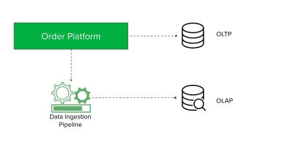
The first design principle towards a stable and scalable database solution is to use different databases to serve transactional and analytical queries, also known as OLTP and OLAP queries. An OLTP database serves queries critical to online order processing. This table keeps data for only a short period of time. Meanwhile, an OLAP database has the same set of data, but serves our historical and statistical queries. This database keeps data for a longer time.

What are the benefits from this design principle? From a stability point of view, we can choose different databases which can better fulfil our different query patterns and QPS requirements. An OLTP database is the single source of truth for online order processing; any failure in the OLAP database will not affect online transactions. From a scalability and cost point of view, we can choose a flexible database for OLAP to support our fast evolution of business requirements. We can maintain less data in our OLTP database while keeping some older data in our OLAP database.

To ensure that the data in both databases are consistent, we introduced the second design principle – data ingestion pipeline. In Figure 1, Order Platform writes data to the OLTP database to process online orders and asynchronously pushes the data into the data ingestion pipeline. The data ingestion pipeline ensures that the OLAP database data is eventually consistent.

Figure 1: Order Platform database solution overview

Architecture details

OLTP database

There are two categories of OLTP queries, the key-value queries (for example, load by order id) and the batch queries (for example, Get ongoing orders by passenger id). We use DynamoDB as the database to support these OLTP queries.

Why DynamoDB?

  1. Scalable and highly available: the tables of DynamoDB are partitioned and each partition is three-way replicated.
  2. Support for strong consistent reads by primary key.
  3. DynamoDB has a mechanism called adaptive capacity to handle hotkey traffic. Internally, DynamoDB will distribute higher capacity to high-traffic partitions, and isolate frequently accessed items to a dedicated partition. This way, the hotkey can utilise the full capacity of an entire partition, which is up to 3000 read capacity units and 1000 write capacity units.
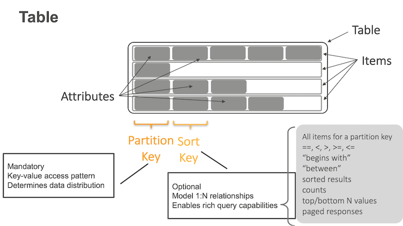
Figure 2: DynamoDB table structure overview. Source: Amazon Web Services (2019, 28 April)

In each DynamoDB table, it has many items with attributes. In each item, it has a partition key and sort key. The partition key is used for key-value queries, and the sort key is used for range queries. In our case, the table contains multiple order items. The partition key is order ID. We can easily support key-value queries by the partition key.

order_id (PK) state pax_id created_at pax_id_gsi
order1 Ongoing Alice 9:00am
order2 Ongoing Alice 9:30am
order3 Completed Alice 8:30am

Batch queries like ‘Get ongoing orders by passenger id’ are supported by DynamoDB Global Secondary Index (GSI). A GSI is like a normal DynamoDB table, which also has keys and attributes.

In our case, we have a GSI table where the partition key is the pax_id_gsi. The attribute pax_id_gsi is linked to the main table. It is eventually consistent with the main table that is maintained by DynamoDB. If the Order Platform queries ongoing orders for Alice, two items will be returned from the GSI table.

pax_id_gsi (PK) created_at (SK) order_id
Alice 9:00am order1
Alice 9:30am order2

We also make use of an advanced feature of GSI named sparse index to support ongoing order queries. When we update order status from ongoing to completed, at the same time, we set the pax_id_gsi to empty, so that the linked item in the GSI will be automatically deleted by DynamoDB. At any time, the GSI table only stores the ongoing orders. We use a sparse index mechanism to control our table size for better performance and to be more cost effective.

The next problem is data retention. This is achieved with the DynamoDB Time To Live (TTL) feature. DynamoDB will auto-scan expired items and delete them. But the challenge is when we add TTL to big tables, it will bring a heavy load to the background scanner and might result in an outage. Our solution is to only add a TTL attribute to the new items in the table. Then, we manually delete the items without TTL attributes, and run a script to delete items with TTL attributes that are too old. After this process, the table size will be quite small, so we can enable the TTL feature on the TTL attribute that we previously added without any concern. The retention period of our DynamoDB data is three months.

Costwise, DynamoDB is charged by storage size and the provision of the read write capability. The provision capability is actually auto scalable. The cost is on-demand. So it’s generally cheaper than RDS.

OLAP database

We use MySQL RDS as the database to support historical and statistical OLAP queries.

Why not Aurora? We choose RDS mainly because it is a mature database solution. Even if Aurora can provide better high-availability, RDS is enough to support our less critical use cases. Costwise, Aurora charges by data storage and the number of requested Input/Output Operations per Second (IOPS). RDS charges only by data storage. As we are using General Purpose (SSD) storage, IOPS is free and supports up to 16k IOPS.

We use MySQL partitioning for data retention. The order table is partitioned by creation time monthly. Since the data access pattern is mostly by month, the partition key can reduce cross-partition queries. Partitions older than six months are dropped at the beginning of each month.

Data ingestion pipeline

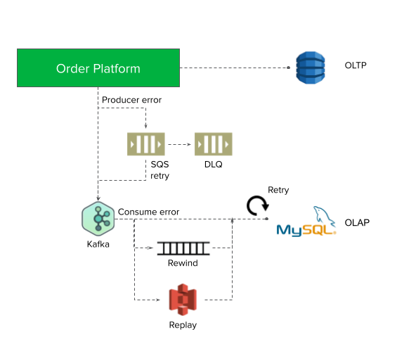
Figure 3: Data Ingestion Pipeline Architecture.

A Kafka stream is used to process data in the data ingestion pipeline. We choose the Kafka stream, because it has 99.95% SLA. It is not restricted by the OLTP and OLAP database types.

Even if Kafka can provide 99.95% SLA, there is still the chance of stream producer failures. When the producer fails, we will store the message in an Amazon Simple Queue Service (SQS) and retry. If the retry also fails, it will be moved to the SQS dead letter queue (DLQ), to be consumed at a later time.

On the stream consumer side, we use back-off retry at both stream and database levels to ensure consistency. In a worst-case scenario, we can rewind the stream events from Kafka.

It is important for the data ingestion pipeline to handle duplicate messages and out-of-order messages.

Duplicate messages are handled by the database level unique key (for example, order ID + creation time).

For the out-of-order messages, we implemented the following two mechanisms:

  1. Version update: we only update the most recently updated data. The precision of the update time is in microseconds, which is enough for most of the use cases.
  2. Upsert: if the update events occur before the create events, we simulate an upsert operation.

Impact

After launching our solution this year, we have saved significantly on cloud costs. In the earlier solution, Order Platform synchronously writes to DynamoDB and Aurora and the data is kept forever.

Conclusion

In terms of stability, we use DynamoDB as the critical OLTP database to ensure high availability for online order processing. Scalability wise, we use RDS as the OLAP database to support our quickly evolving business requirements by using a rich, multiple index. Cost efficiency is achieved by data retention in both databases. For consistency, we built a single source of truth OLTP database and an OLAP database that is eventually consistent with the help of the data ingestion pipeline.

What’s next?

Currently, the database solution is running on the production environment. Even though the database solution is proven to be stable, scalable and consistent, we still see some potential areas of improvement.

We use MySQL RDS for OLAP data storage. Even though MySQL is stable and cost effective, it is difficult to serve more complicated queries like free text search. Hence, we plan to explore other NoSQL databases like ElasticSearch.

We hope this post helps you understand how we store Grab orders and fulfil the queries from the Grab Order Platform.

References

Amazon Web Services. (2019, 28 April) Build with DynamoDB: S1 E1 – Intro to Amazon DynamoDB [Video]. YouTube.

Join us

Grab is the leading superapp platform in Southeast Asia, providing everyday services that matter to consumers. More than just a ride-hailing and food delivery app, Grab offers a wide range of on-demand services in the region, including mobility, food, package and grocery delivery services, mobile payments, and financial services across 428 cities in eight countries.

Powered by technology and driven by heart, our mission is to drive Southeast Asia forward by creating economic empowerment for everyone. If this mission speaks to you, join our team today!
Optimally scaling Kafka consumer applications

Post Syndicated from Grab Tech original https://engineering.grab.com/optimally-scaling-kafka-consumer-applications

Earlier this year, we took you on a journey on how we built and deployed our event sourcing and stream processing framework at Grab. We’re happy to share that we’re able to reliably maintain our uptime and continue to service close to 400 billion events a week. We haven’t stopped there though. To ensure that we can scale our framework as the Grab business continuously grows, we have spent efforts optimizing our infrastructure.

In this article, we will dive deeper into our Kubernetes infrastructure setup for our stream processing framework. We will cover why and how we focus on optimal scalability and availability of our infrastructure.

Quick Architecture Recap

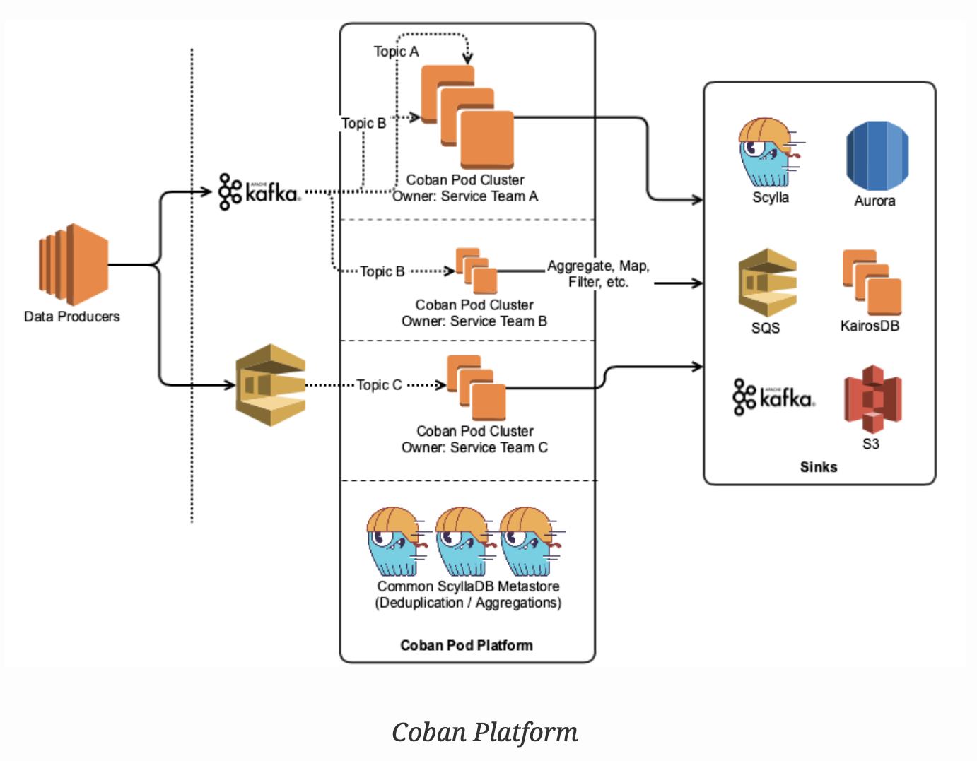
Coban Platform Architecture

The Coban platform provides lightweight Golang plugin architecture-based data processing pipelines running in Kubernetes. These are essentially Kafka consumer pods that consume data, process it, and then materialize the results into various sinks (RDMS, other Kafka topics).

Anatomy of a Processing Pod

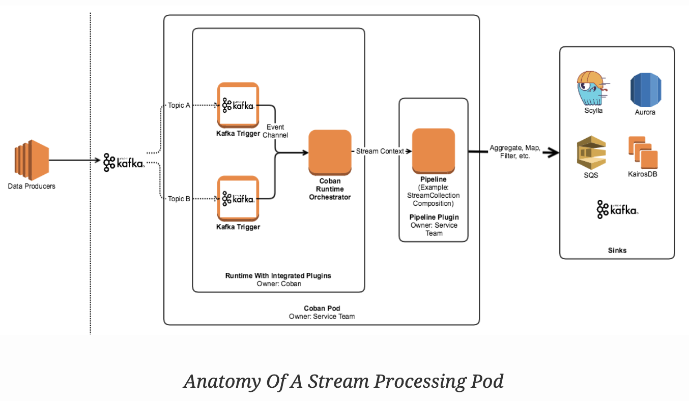
Anatomy of a Processing Pod

Each stream processing pod (the smallest unit of a pipeline’s deployment) has three top level components:

  • Trigger: An interface that connects directly to the source of the data and converts it into an event channel.
  • Runtime: This is the app’s entry point and the orchestrator of the pod. It manages the worker pools, triggers, event channels, and lifecycle events.
  • Pipeline plugin: This is provided by the user, and conforms to a contract that the platform team publishes. It contains the domain logic for the pipeline and houses the pipeline orchestration defined by a user based on our Stream Processing Framework.

Optimal Scaling

We initially architected our Kubernetes setup around horizontal pod autoscaling (HPA), which scales the number of pods per deployment based on CPU and memory usage. HPA keeps CPU and memory per pod specified in the deployment manifest and scales horizontally as the load changes.

These were the areas of application wastage we observed on our platform:

  • As Grab’s traffic is uneven, we’d always have to provision for peak traffic. As users would not (or could not) always account for ramps, they would be fairly liberal with setting limit values (CPU and memory), leading to resource wastage.
  • Pods often had uneven traffic distribution despite fairly even partition load distribution in Kafka. The Stream Processing Framework(SPF) is essentially Kafka consumers consuming from Kafka topics, hence the number of pods scaling in and out resulted in unequal partition load per pod.

Vertically Scaling with Fixed Number of Pods

We initially kept the number of pods for a pipeline equal to the number of partitions in the topic the pipeline consumes from. This ensured even distribution of partitions to each pod providing balanced consumption. In order to abstract this from the end user, we automated the application deployment process to directly call the Kafka API to fetch the number of partitions during runtime.

After achieving a fixed number of pods for the pipeline, we wanted to move away from HPA. We wanted our pods to scale up and down as the load increases or decreases without any manual intervention. Vertical pod autoscaling (VPA) solves this problem as it relieves us from any manual operation for setting up resources for our deployment.

We just deploy the application and let VPA handle the resources required for its operation. It’s known to not be very susceptible to quick load changes as it trains its model to monitor the deployment’s load trend over a period of time before recommending an optimal resource. This process ensures the optimal resource allocation for our pipelines considering the historic trends on throughput.

We saw a ~45% reduction in our total resource usage vs resource requested after moving to VPA with a fixed number of pods from HPA.

Anatomy of a Processing Pod

Managing Availability

We broadly classify our workloads as latency sensitive (critical) and latency tolerant (non-critical). As a result, we could optimize scheduling and cost efficiency using priority classes and overprovisioning on heterogeneous node types on AWS.

Kubernetes Priority Classes

The main cost of running EKS in AWS is attributed to the EC2 machines that form the worker nodes for the Kubernetes cluster. Running On-Demand brings all the guarantees of instance availability but it is definitely very expensive. Hence, our first action to drive cost optimisation was to include Spot instances in our worker node group.

With the uncertainty of losing a spot instance, we started assigning priority to our various applications. We then let the user choose the priority of their pipeline depending on their use case. Different priorities would result in different node affinity to different kinds of instance groups (On-Demand/Spot). For example, Critical pipelines (latency sensitive) run on On-Demand worker node groups and Non-critical pipelines (latency tolerant) on Spot instance worker node groups.

We use priority class as a method of preemption, as well as a node affinity that chooses a certain priority pipeline for the node group to deploy to.

Overprovisioning

With spot instances running we realised a need to make our cluster quickly respond to failures. We wanted to achieve quick rescheduling of evicted pods, hence we added overprovisioning to our cluster. This means we keep some noop pods occupying free space running in our worker node groups for the quick scheduling of evicted or deploying pods.

The overprovisioned pods are the lowest priority pods, thus can be preempted by any pod waiting in the queue for scheduling. We used cluster proportional autoscaler to decide the right number of these overprovisioned pods, which scales up and down proportionally to cluster size (i.e number of nodes and CPU in worker node group). This relieves us from tuning the number of these noop pods as the cluster scales up or down over the period keeping the free space proportional to current cluster capacity.

Lastly, overprovisioning also helped improve the deployment time because there is no  dependency on the time required for Auto Scaling Groups (ASG) to add a new node to the cluster every time we want to deploy a new application.

Future Improvements

Evolution is an ongoing process. In the next few months, we plan to work on custom resources for combining VPA and fixed deployment size. Our current architecture setup works fine for now, but we would like to create a more tuneable in-house CRD(Custom Resource Definition) for VPA that incorporates rightsizing our Kubernetes deployment horizontally.


Authored By Shubham Badkur on behalf of the Coban team at Grab – Ryan Ooi, Karan Kamath, Hui Yang, Yuguang Xiao, Jump Char, Jason Cusick, Shrinand Thakkar, Dean Barlan, Shivam Dixit, Andy Nguyen, and Ravi Tandon.


Join us

Grab is more than just the leading ride-hailing and mobile payments platform in Southeast Asia. We use data and technology to improve everything from transportation to payments and financial services across a region of more than 620 million people. We aspire to unlock the true potential of Southeast Asia and look for like-minded individuals to join us on this ride.

If you share our vision of driving South East Asia forward, apply to join our team today.