In the blog our previous introduction to the SOP-driven LLM Agent Framework, we the potential of LLM agent framework to revolutionise business operations was discussed. Now, we’re excited to explore a compelling use case: automating Account Takeover (ATO) investigations in Risk Operations (RiskOps). This framework has significantly reduced manual effort, improved efficiency, and minimised errors in the investigation process, setting a new standard for secure and streamlined operations.
The challenge in RiskOps
Traditionally, ATO investigations have been fraught with challenges due to their complexity and the manual effort required. Analysts must sift through vast amounts of data, cross-referencing multiple systems and executing numerous SQL queries to make informed decisions. This process is not only labor-intensive but also susceptible to human error, which can lead to inconsistencies and potential security breaches.
The manual approach often involves:
Time-consuming data analysis: Analysts spend significant time gathering and interpreting data from disparate sources, leading to delays and inefficiencies.
Decision fatigue: Continuous decision-making in a high-pressure environment can result in oversight or errors, especially when relying on predefined thresholds without adaptive insights.
Resource constraints: The need for specialised skills to handle SQL queries and interpret complex patterns limits the scalability of the process.
These challenges highlight the need for a more efficient, reliable, and scalable solution.
Leveraging the SOP agent framework
Our framework transforms the ATO investigation process by mirroring manual workflows while leveraging advanced automation.
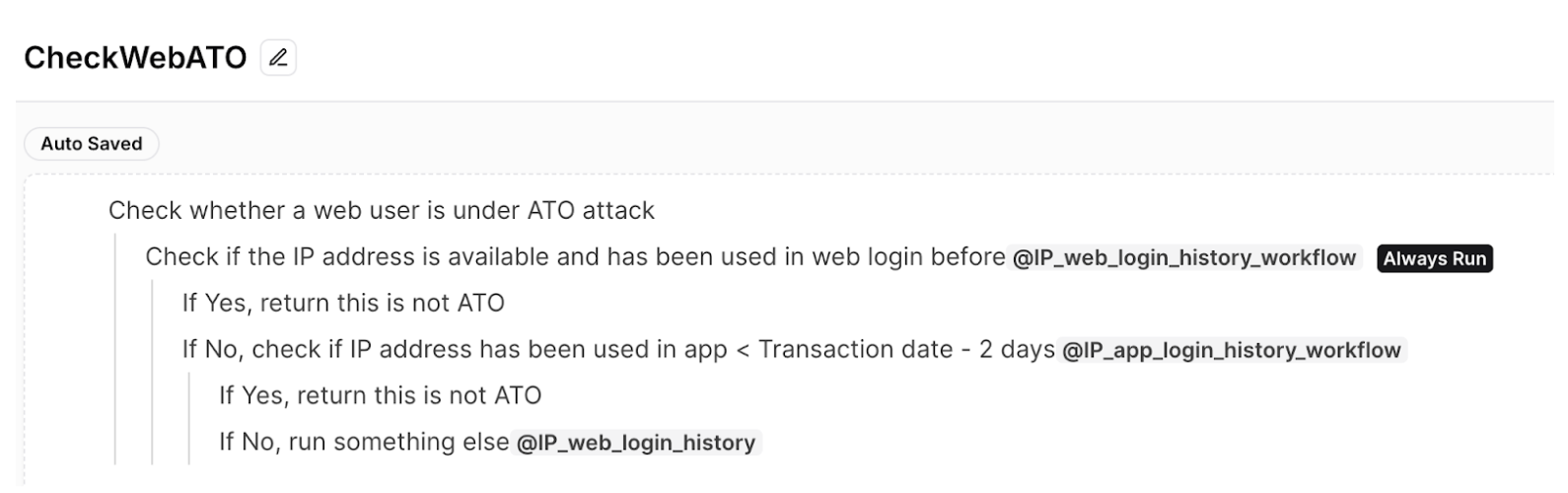
At its core, a Standard Operating Procedure (SOP) guides the investigation process. This comprehensive SOP, is designed with an intuitive tree structure. It outlines the sequence of investigative actions, required data for each step, necessary SQL queries and external function calls, as well as decision criteria guiding the investigation. Figure 1 shows the example of ATO investigation SOP.
Figure 1: Example of fictional ATO investigation SOP
The SOP is written in natural language in an indentation format. Users can easily define SOPs using an intuitive editor. This format also clearly denotes the specific functions or queries associated with each step in the SOP. The @function_name notation (eg. @IP_web_login_history) makes it easy to identify where external calls are made within the process, highlighting the integration points between the SOP-driven LLM agent framework and the existing systems or databases.
Dynamic execution
The dynamic execution engine consists of the SOP planner and the Worker Agent, working in tandem to drive efficient operations. The SOP planner serves as the navigator, guiding the investigation’s path by generating the necessary SOP steps and determining the appropriate APIs to call. It uses a structured execution approach inspired by Depth-First Search (DFS) to ensure thorough and systematic processing. Meanwhile, the Worker Agent acts as the executor, interpreting the JSON-formatted SOPs, invoking required APIs or SQL queries, and storing results. This continuous interplay between the SOP planner and the Worker Agent establishes an efficient feedback loop, propelling the investigation forward with precision and reliability.
The automated investigation process begins at the root of the SOP tree and methodically progresses through each defined step. At each juncture, the system executes specified SQL queries as needed, retrieving and analysing relevant data. Based on this analysis, the framework evaluates step specific criteria and makes informed decisions that guide subsequent steps. This iterative process allows the investigation to delve as deeply into the data as the SOP dictates, ensuring both thoroughness and efficiency.
As the investigation concludes, having completed all of the steps, the framework enters its final phase. It compiles a comprehensive summary of the entire process, synthesising all gathered information to generate a final decision. The culmination of this process is a detailed report that encapsulates the investigation’s findings and provides clear, actionable conclusions.
This automated approach combines the best of human expertise with computational efficiency. It maintains the depth and detail of a human-conducted investigation while leveraging the speed and consistency of automation. The result is a powerful tool that can handle complex investigations with precision and reliability, making it an invaluable asset in various fields requiring thorough and systematic analysis.
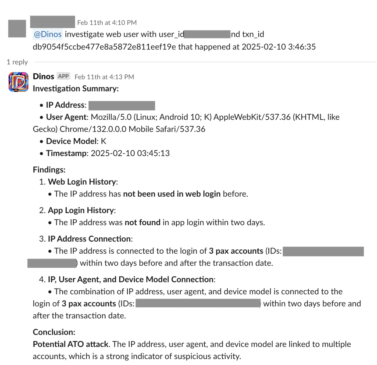
Figure 2: Example of dynamic execution
Efficiency, impact and future potential
The SOP-driven LLM agent framework has demonstrated remarkable efficiency and impact in automating RiskOps processes. By automating data handling and leveraging AI to adapt to emerging patterns, the framework has significantly reduced manual tasks and streamlined operations. Figure 3 shows an example of an automated RiskOps process integrated with Slack.
Figure 3: Slack integration
Key achievements of automating RiskOps process:
Reduction in handling time from 22 to 3 minutes per ticket.
Automation of 87% of ATO cases since launch.
Achievement of a zero-error rate, enhancing both efficiency and security.
These results not only demonstrate the framework’s effectiveness in streamlining RiskOps but also provide stakeholders with increased confidence in the security and reliability of their operations.
The success of the framework in automating ATO investigations opens the door to a wider range of applications across various sectors. By adapting the framework to different processes, organisations can achieve similar improvements in efficiency and reliability, leading to a more responsive and agile business environment.
Conclusion
The SOP-driven LLM agent framework is more than an automation tool. It’s a catalyst for transforming enterprise operations. By applying it to ATO investigations, we’ve demonstrated its potential to enhance efficiency, reliability, and security. As we continue to explore its capabilities, we anticipate unlocking new levels of productivity and innovation across industries.
We look forward to sharing more as we explore how this groundbreaking framework can be applied to various challenges, helping organisations navigate the complexities of modern operations with confidence and precision.
Join us
Grab is a leading superapp in Southeast Asia, operating across the deliveries, mobility and digital financial services sectors. Serving over 800 cities in eight Southeast Asian countries, Grab enables millions of people everyday to order food or groceries, send packages, hail a ride or taxi, pay for online purchases or access services such as lending and insurance, all through a single app. Grab was founded in 2012 with the mission to drive Southeast Asia forward by creating economic empowerment for everyone. Grab strives to serve a triple bottom line – we aim to simultaneously deliver financial performance for our shareholders and have a positive social impact, which includes economic empowerment for millions of people in the region, while mitigating our environmental footprint.
Powered by technology and driven by heart, our mission is to drive Southeast Asia forward by creating economic empowerment for everyone. If this mission speaks to you, join our team today!
We’re excited to introduce an innovative Large Language Model (LLM) agent framework that reimagines how enterprises can harness the power of AI to streamline operations and boost productivity. At its core, this framework leverages Standard Operating Procedures (SOPs) to guide AI-driven execution, ensuring reliability and consistency in complex processes. Initial evaluations have shown remarkable results, with over 99.8% accuracy in real-world use cases. For example, the framework has powered solutions like the Account Takeover Investigations (ATI) bot, which achieved a 0 false rate while reducing investigation time from 23 minutes to just 3, automating 87% of cases. The fraud investigation use case also reduced the average handling time (AHT) by 45%, saving over 300 man-hours monthly with a 0 false rate, demonstrating its potential to transform even the most intricate enterprise operations with a high degree of accuracy.
The framework’s capabilities extend far beyond just accuracy, it offers a versatile suite of tools that revolutionise automation and app development, enabling AI-powered solutions up to 10 times faster than traditional methods.
The power of SOPs in AI automation
Traditional agent-based applications often use LLMs as the core controller to navigate through standard operating procedure (SOPs). However, this approach faces several challenges. LLMs may make incorrect decisions or invent non-existent steps due to hallucination. As generative models, they struggle to consistently produce results in a fixed format. Moreover, navigating complex SOPs with multiple branching pathways is particularly challenging for LLMs. These issues can lead to inefficiencies and inaccuracies in implementing business operations, especially when dealing with intricate, multi-step procedures.
Our framework addresses these challenges head-on by leveraging the structure and reliability of SOPs. We represent SOPs as a tree, with nodes encapsulating individual actions or decision points. This structure supports both sequential and conditional branching operations, mirroring the hierarchical nature of real-world business processes.
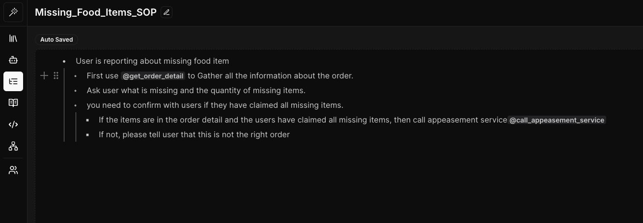
To make this powerful tool accessible to all, we’ve developed an intuitive SOP editor that allows non-technical users to easily define and visualise complex workflows. These visual representations are then converted into a structured, indented format that our system can interpret and execute efficiently.
Figure 1: SOP editor in our framework
The example above demonstrates how our framework transforms the customer support process by mirroring manual workflows while leveraging advanced automation. The SOP is written in natural language using an indentation format, making it easy for users to define and understand. The @function_name (@get_order_detail) notation clearly identifies where external calls are made within the process, highlighting the integration points between the SOP-driven LLM agent framework and existing systems or databases.
The magic behind the scenes
The framework’s strength lies in the synergy between three key components: the planner module, LLM-powered worker agent, and user agent. This intelligent trio works in harmony to deliver a seamless, efficient, and adaptable automation experience.
The planner module employs a Depth-First Search (DFS) algorithm to navigate the SOP tree, ensuring thorough execution with step-by-step prompt generation and sophisticated backtracking mechanisms. The LLM-powered worker agent dynamically updates its understanding and makes decisions based on the most current information. Our approach tackles hallucination and improves efficiency through context compression and strategic limitation of available Application Programming Interface tools (APIs). The framework’s dynamic branching capability allows for adaptive navigation based on real-time data and analysis.
Serving as the primary user interface, the user agent offers multilingual interaction, accurate intent identification, and seamless handling of out-of-order scenarios.
By combining structured SOPs with flexible LLM-powered agents and advanced algorithmic approaches, our framework adeptly handles complex, real-world scenarios while maintaining reliability and consistency. This innovative architecture effectively mitigates common LLM challenges, resulting in a robust system capable of navigating intricate business processes with high accuracy and adaptability.
Beyond SOPs: A suite of powerful features
While SOPs form the backbone of our framework, we’ve incorporated several other cutting-edge features to create a truly comprehensive solution. Our Graph Retrieval-Augmented Generation (GRAG) pipeline enhances information retrieval and content generation tasks, allowing for more accurate and context-aware responses. The workflow feature enables chaining multiple plugins together to handle complex processes effortlessly, improving efficiency across various departments.
Our plugin system seamlessly integrates with various technologies such as API, Python, and SQL, providing the flexibility to meet diverse needs. Whether you’re an engineer coding in Python, a data analyst working with SQL, or a risk operations specialist, our plugin system adapts to your preferred tools. Additionally, our playground feature allows users to develop, test, and refine LLM applications easily in an interactive environment, supporting the latest multi-modal APIs for accelerated innovation.
Figure 2: Workflow builder feature in our framework
Empowering teams through versatility and accessibility
Our framework is designed to empower teams across the organisation. The multilingual capabilities of our user agent ensure that language barriers don’t hinder adoption or efficiency. For scenarios requiring human intervention, we’ve implemented a state stack that allows for pausing and resuming execution seamlessly. This feature ensures that complex processes can be handled with the right balance of automation and human oversight.
Security and transparency at the forefront
In an era where data security and process transparency are paramount, our framework doesn’t fall short. It’s designed with a security-first approach, ensuring granular access control so that users only access information they’re authorised to see. Additionally, we provide detailed logging and visualisation of each execution, offering complete explainability of the automation process. This level of transparency not only aids in troubleshooting but also helps in building trust in the AI-driven processes across the organisation.
Looking ahead
As we continue to refine and expand this LLM agent framework, we’re excited to explore its potential across different industries. We’ll be sharing more about each of these features in the future and showcase how they can be leveraged to solve specific business challenges and explore real-world applications.
Look forward to more in-depth explorations of the framework’s capabilities, use cases, and technical innovations. With this revolutionary approach, you’re not just automating tasks – you’re transforming the way your enterprise operates, unleashing the true power of LLM in your organisation.
Join us
Grab is a leading superapp in Southeast Asia, operating across the deliveries, mobility and digital financial services sectors. Serving over 800 cities in eight Southeast Asian countries, Grab enables millions of people everyday to order food or groceries, send packages, hail a ride or taxi, pay for online purchases or access services such as lending and insurance, all through a single app. Grab was founded in 2012 with the mission to drive Southeast Asia forward by creating economic empowerment for everyone. Grab strives to serve a triple bottom line – we aim to simultaneously deliver financial performance for our shareholders and have a positive social impact, which includes economic empowerment for millions of people in the region, while mitigating our environmental footprint.
Powered by technology and driven by heart, our mission is to drive Southeast Asia forward by creating economic empowerment for everyone. If this mission speaks to you, join our team today!
Hugo plays a pivotal role in enabling data ingestion for Grab’s data lake, managing over 4,000 pipelines onboarded by users. The stability of Hugo pipelines is contingent upon the health of both the data sources and various Hugo components. Given the complexity of this system, pipeline failures occasionally occur, necessitating user intervention when retry mechanisms prove insufficient. These incidents present challenges such as:
Limited user visibility into pipeline issues.
Uncertainty about resolution steps due to extensive documentation.
An overwhelmed Hugo on-call team dealing with ad-hoc requests and growing infrastructure dependencies.
Raised Data Production Issues (DPIs) lacking clear Root Cause Analysis (RCA), hindering effective management.
Such challenges ultimately increase data downtime due to prolonged issue triage and resolution times.
To address these problems, we conducted a thorough analysis of failure modes and the efforts required to resolve them. Based on our findings, we propose a comprehensive automation solution.
This blog outlines the architecture and implementation of our proposed solution, consisting of modules like Signal, Diagnosis, RCA Table, Auto-resolution, Data Health API, and Data Health WorkBench, each with a specific function to enhance Hugo’s monitoring, diagnosis, and resolution capabilities.
The blog further details the impact of these automated features, such as enhanced data visibility, reduced on-call workload, and concludes with our next steps, which focus on advancing auto-resolution strategies, enriching the Data Health Workbench, and broadening diagnostics to include more infrastructure components, like Flink, for comprehensive coverage.
Architecture details
We designed the solution based on these principles:
Identify different failure modes based on past issues and analysis from first principles.
Analyse temporal relationships of pipeline execution steps to diagnose issues to failure modes.
Focus on auto-resolution, and add additional features to cover gaps which can’t be immediately addressed by auto-resolution or diagnosis.
The following diagram shows the solution we proposed.
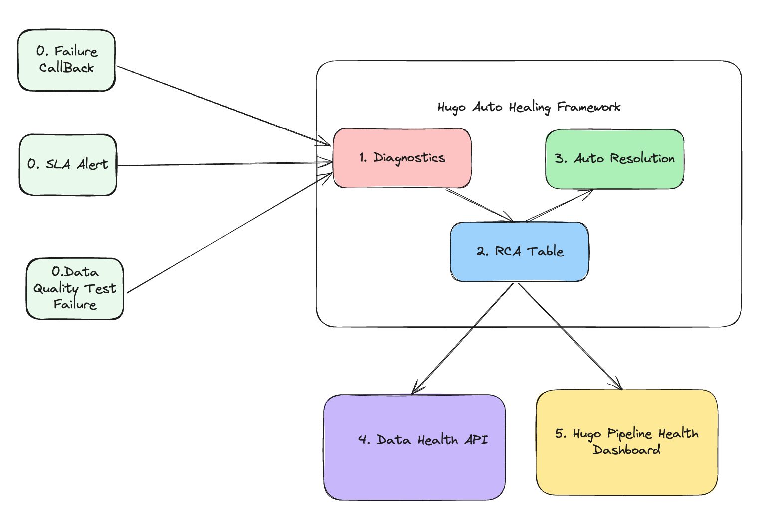
Figure 1. Architecture
The architecture consists of five core modules, each with a specific function:
Signal module: This module is responsible for collecting signals. It gathers three different types of signals that collectively define the health status of the data lake table. The signals include:
Failure callback signal: This indicates whether the pipeline runs involving this data lake table are successful or not.
SLA alert signal: This indicates whether the pipeline execution involving this data lake table meets the Service Level Agreement (SLA). For an hourly batch job, the expectation is to complete within one hour.
Data quality test failure signal: This represents various types of completeness checks to ensure that data lake tables are consistent with the source tables based on their pipeline strategies.
Diagnosis module: This is the core module responsible for diagnosing the root cause of 3 types of failures collected in the Signal module. It determines:
The root cause of the failure.
The assignee responsible for fixing the error.
The auto-resolution method to fix the issue.
Manual resolution steps if the auto-resolution fails.
RCA table: This module stores the following information:
Signals
Assignee information
Diagnosis results
Auto-resolution methods
Manual resolution steps
Auto-resolution module: This module executes the auto-resolution methods to resolve issues automatically.
Data health API: This module provides API access to other platforms. External platforms or pipelines that rely on Hugo onboarded tables can subscribe to the health status and investigate the root cause when a table is deemed unhealthy.
Hugo pipeline health dashboard: A centralised dashboard for Hugo users to visualise the health status of tables, auto resolution status, and manual fix button.
By leveraging these modules, the architecture ensures robust monitoring, diagnosis, and resolution of issues, leading to improved data health and operational efficiency.
Implementation
Signal module
There are two methods for generating these three signals. The failure signal is generated through an airflow callback, while the SLA miss and data completeness test signals are produced by Genchi. Genchi is a data quality observability platform at Grab that performs data quality checks and acts as a crucial enabler for the enforcement of data contracts.
Diagnosis module
As soon as an alert is created, the diagnosis begins. To avoid lengthy diagnosis times, Hugo has developed an innovative approach that eliminates the requirement for parsing extensive logs, such as Spark executor logs or Airflow logs. Instead, it gathers signals transmitted by the computation engine or Grab’s internal platforms.
The diagnosis process can be time-consuming, even with efforts to reduce the time it takes. For example, the SLA diagnoser uses multiple analysers that run sequentially, and some of these analysers (like the Airflow analyser) make API calls that can take a significant amount of time. The more analysers that are involved in the diagnosis process, the longer it can take.
Figure 2. Diagnosis process
Parallelism in diagnosis serves as a solution to lower the overall latency when there is a surge in error traffic. The degree of parallelism differs based on the type of signal. For example, the failure signal diagnosis can be executed in thousands of processes at once, while for SLA miss and data quality test failures signals, the parallelism is determined by the number of partitions in the Kafka topic since these signals are received from Kafka.
Auto-resolution module
Auto-resolution is a flexible framework that enables the implementation of custom handlers for various types of failures. One of the common handlers employs a retry mechanism with backoff for transient errors. For instance, if Hugo receives a failure callback indicating that the root cause is a database replica lag, it would wait for an hour before re-triggering the job. This auto-resolution process runs asynchronously with the diagnosis process.
Data health API
The data health information includes a unique identifier, current status, error details, and the time of the last health check, providing a comprehensive snapshot of the dataset’s health.
Hugo converts the detailed information available in its internal data health API to the data health API specification format to be consumed by Kinabalu, our internal system designed to automate and streamline incident management processes by integrating with multiple systems such as Slack, Jira, Splunk on-call, and Datadog.
Hugo pipeline health dashboard
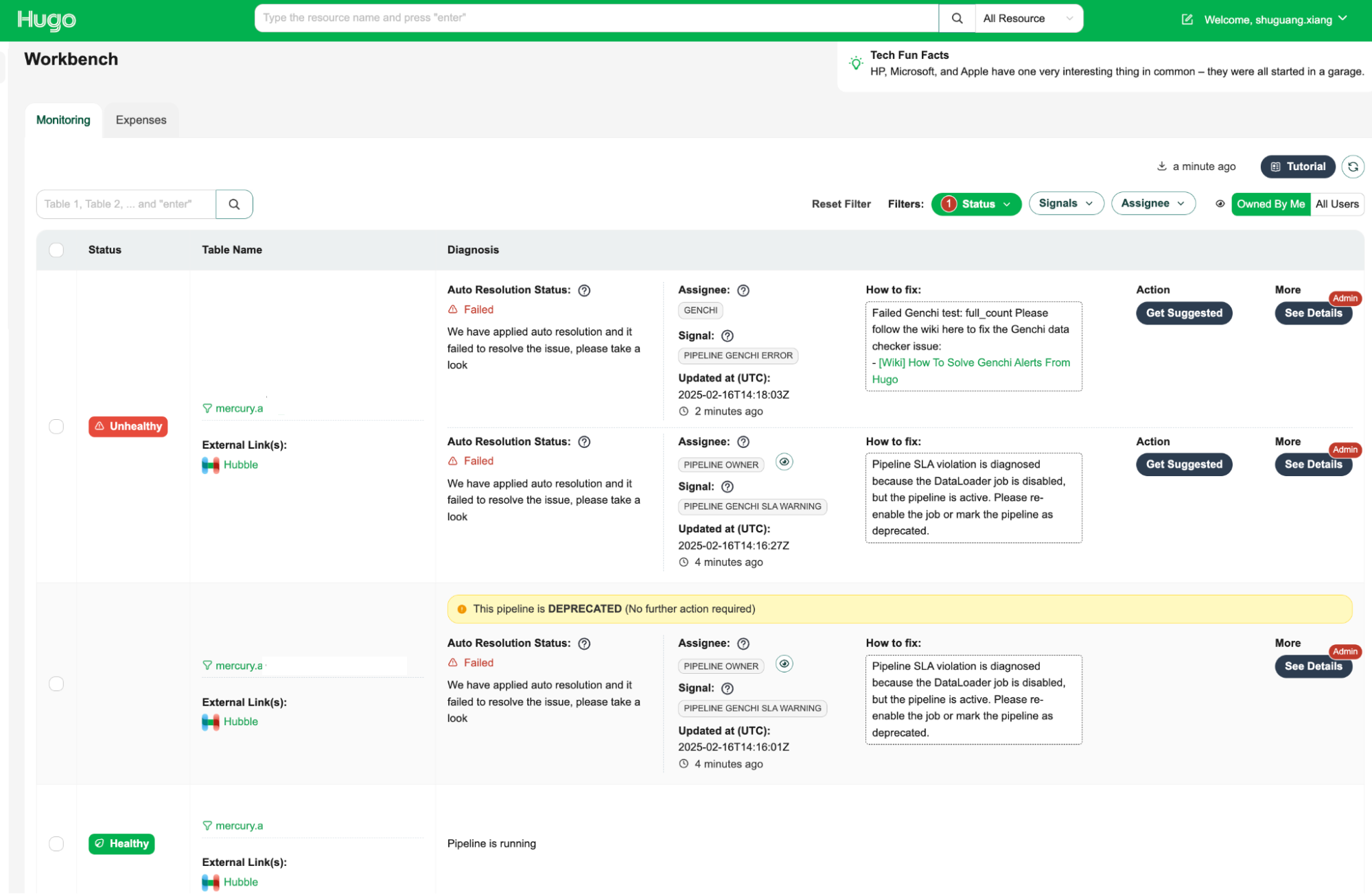
The Data Health Workbench is a centralised dashboard for Hugo users to visualise the health status of tables, auto-resolution status, and manual fix buttons. It provides a comprehensive view of data health and facilitates efficient issue resolution.
The key features are as follows:
Health status visualisation: Displays the current health status of tables, making it easy to identify unhealthy tables.
Assignee information: Indicates the assignee responsible for fixing the issue, ensuring clear accountability.
How-to-fix guide: Provides step-by-step instructions on how to resolve the issue, empowering users to take immediate action.
Action: Offers an action button to initiate the resolution process with a single click, streamlining issue resolution.
Admin feature with detailed diagnosis information: Provides admins supplementary information, including the reasoning behind the root cause identification and assignee determination, which allows for a deeper understanding of the root cause of issues.
By leveraging the Data Health Workbench, Hugo users can efficiently monitor and manage data health, ensuring data integrity and operational efficiency.
Figure 3. Data Health Workbench
Impact
The implementation of Hugo’s auto-healing and diagnosis features has resulted in significant improvements in stability and operational efficiency for our data pipelines. Here are some key outcomes:
Enhanced data visibility: We’ve improved the visibility into the health of datasets, allowing for quick identification of issues and more informed decision-making.
Timely resolution of data issues: With automated diagnostic and resolution processes, we ensure that data issues are addressed promptly, minimising data downtime and enhancing overall data availability.
Reduced on-call workload: By automating many of the common failure resolutions, the workload on Hugo on-call teams has been significantly reduced. This allows teams to focus on more complex and impactful tasks.
Scalable solution for managing complexity: The auto-resolution framework is well-equipped to handle the increasing complexity of data infrastructure, offering scalable solutions for transient errors through custom handlers and retry mechanisms.
Improved data contract management: By providing detailed pipeline health information via the Data Health API, we enable precise and accurate DPIs, complete with root cause analysis and assignee information, enhancing the management and resolution of data contract breaches.
Valuable reference for other platforms: The insights and methodologies developed through this initiative provide a valuable reference for other platform teams at Grab looking to implement similar automation and diagnostic capabilities.
Support for Grab’s success: These enhancements support Grabbers by ensuring easy access to the datasets they need and contribute to the overall success of Grab through reliable data availability.
Next steps
Our next steps involve advancing auto-resolution strategies by focusing on complex solutions like pipeline runtime optimisation to boost efficiency and minimise processing delays. We will enrich the Data Health Workbench with detailed information, enabling users to visualise and understand pipeline health more effectively and make informed corrective actions. Additionally, we plan to broaden our diagnosis capabilities by integrating more infrastructure components, such as Flink health information, to ensure a comprehensive and holistic monitoring approach for all engines within Hugo.
Join us
Grab is a leading superapp in Southeast Asia, operating across the deliveries, mobility and digital financial services sectors. Serving over 800 cities in eight Southeast Asian countries, Grab enables millions of people everyday to order food or groceries, send packages, hail a ride or taxi, pay for online purchases or access services such as lending and insurance, all through a single app. Grab was founded in 2012 with the mission to drive Southeast Asia forward by creating economic empowerment for everyone. Grab strives to serve a triple bottom line – we aim to simultaneously deliver financial performance for our shareholders and have a positive social impact, which includes economic empowerment for millions of people in the region, while mitigating our environmental footprint.
Powered by technology and driven by heart, our mission is to drive Southeast Asia forward by creating economic empowerment for everyone. If this mission speaks to you, join our team today!
At Grab, we’ve been working to perfect our Spark observability tools. Our initial solution, Iris, was developed to provide a custom, in-depth observability tool for Spark jobs. As described in our previous blog post, Iris collects and analyses metrics and metadata at the job level, providing insights into resource usage, performance, and query patterns across our Spark clusters.
Iris addresses a critical gap in Spark observability by providing real-time performance metrics at the Spark application level. Unlike traditional monitoring tools that typically provide metrics only at the EC2 instance level, Iris dives deeper into the Spark ecosystem. It bridges the observability gap by making Spark metrics accessible through a tabular dataset, enabling real-time monitoring and historical analysis. This approach eliminates the need to parse complex Spark event log JSON files, which users are often unable to access when they need immediate insights. Iris empowers users with on-demand access to comprehensive Spark performance data, facilitating quicker decision-making and more efficient resource management.
Iris served us well, offering basic dashboards and charts that helped our teams understand trends, discover issues, and debug their Spark jobs. However, as our needs evolved and usage grew, we began to encounter limitations:
Fragmented user experience and access control: Observability data is split between Grafana (real-time) and Superset (historical), forcing users to switch platforms for a complete view. The complex Grafana dashboards, while powerful, were challenging for non-technical users. The lack of granular permissions hindered wider adoption. We needed a unified, user-friendly interface with role-based access to serve all Grabbers effectively.
Operational overhead: Our data pipeline for offline analytics includes multiple hops and complex transformations.
Data management: We faced challenges managing real-time data in InfluxDB alongside offline data in our data lake, particularly with string-type metadata.
These challenges and the need for a centralised, user-friendly web application prompted us to seek a more robust solution. Enter StarRocks – a modern analytical database that addresses many of our pain points:
Pain points with InfluxDB
StarRocks solution
Limited SQL compatibility: Requires use of Flux query language instead of full SQL
Full MySQL-compatible SQL support, enabling seamless integration with existing tools and skills
Complex data ingestion pipeline: Requires external agents like Telegraf to consume Kafka and insert into InfluxDB
Direct Kafka ingestion, eliminating the need for intermediate agents and simplifying the data pipeline
Limited pre-aggregation capabilities: Aggregation is limited to time windows and indexed columns, not string columns
Flexible materialised views supporting complex aggregations on any column type, improving query performance
Poor support for metadata and joins: Designed primarily for numerical time series data, with slow performance on string data and joins
Efficient handling of both time-series and string-type metadata in a single system, with optimised join performance
Difficult integration with data lake: There is no official way to backup or stream data directly to the datalake, requiring separate pipelines
Native S3 integration for easy backup and direct data lake accessibility, eliminating the need for separate ingestion pipelines
Performance issues with high cardinality data: Indexing unique identifiers (like app\_id) causes huge indexes and slow queries
Optimised for high cardinality data, allowing efficient querying on unique identifiers without performance degradation
In this blog post, we will dive into leveraging StarRocks to build the next generation of the Spark observability platform. We will explore the architecture, data model, and key features that are helping us overcome previous limitations and provide more value to Spark users at Grab.
System architecture overview
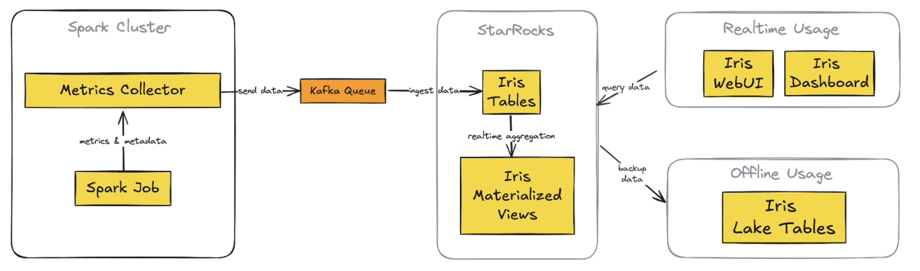
In the journey to enhance user experience, we’ve made substantial changes to the architecture, moving from the Telegraf/InfluxDB/Grafana (TIG) stack to a more streamlined and powerful setup centered around StarRocks. This new architecture addresses the previous challenges and provides a more unified, flexible, and efficient solution.
Figure 1. New Iris architecture with StarRocks integration
Key Components of the new architecture:
1. StarRocks database
Replaces InfluxDB for both real-time and historical data storage
Supports complex queries on metrics and metadata tables
2. Direct Kafka ingestion
StarRocks ingests data directly from Kafka, eliminating Telegraf
3. Custom web application (Iris UI)
Replaces Grafana dashboards
Centralised, flexible interface with custom API
4. Superset integration
Maintained and now connected directly to StarRocks
Provides real-time data access, consistent with the custom web app
5. Simplified offline data process
Scheduled backups from StarRocks to S3 directly
Replaces previous complex data lake pipelines
Key improvements:
1. Unified data store: Single source for real-time and historical data
2. Streamlined data flow: A simplified pipeline reduces latency and failure points
3. Flexible visualisation: Custom web app with intuitive, role-specific interfaces
4. Consistent real-time access: Across both custom app and Superset
5. Simplified backup and data lake integration: Direct S3 backups
Data model and ingestion
The Iris observability system is designed to monitor both job executions and ad-hoc cluster usage, encompassing what we call “cluster observation”. This model accounts for two scenarios:
Adhoc use: Pre-created clusters shared among team users
Job execution: New clusters are created for each job submission
Key design points
For each cluster, we capture both metadata and metrics:
Key point
Description
Linkage
We use worker\_uuid to link metadata with worker metrics app\_id to link metadata with Spark event metrics.
Granularity
Worker metrics are captured every 5 seconds, linked by worker\_uuid. Spark events are captured as they occur, linked by app\_id. Metadata can be captured multiple times.
Flexibility
This schema allows for queries at various levels: Individual worker level, job level, cluster level.
Historical analysis
The design enables insights from historical runs, such as: Auto-scaling behaviour, maximum worker count per job, maximum or average memory usage over time.
We use StarRocks’ routine load feature to ingest data directly from Kafka into our tables. Refer to the StarRocks documentation: Load data using routine load.
Here is a simple example of creating a routine load job for cluster worker metrics:
This configuration sets up continuous data ingestion from the specified Kafka topic into our cluster_worker_metrics table, with JSON parsing.
For monitoring the routine, StarRocks provides built-in tools to monitor the status/error log of routine load jobs. Example query to check load:
    C/C++
    SHOW ROUTINE LOAD WHERE NAME = "iris.routetine_cluster_worker_metrics_raw";
Handle both real-time and historical data in the unified system
The new Iris system uses StarRocks to efficiently manage both real-time and historical data. We have implemented three key features to achieve this:
StarRocks’ routine load enables near real-time data ingestion from Kafka. Multiple load tasks concurrently consume messages from different topic partitions, resulting in data appearing in Iris tables within seconds of collection. This quick ingestion keeps our monitoring capabilities current, providing users with up-to-date information about their Spark jobs.
For historical analysis, StarRocks serves as a persistent dataset, storing metadata and job metrics with a time-to-live of over 30 days. This allows us to perform analysis based on the last 30 days of job runs directly in StarRocks, which is significantly faster than using offline data in our data lake.
We’ve also implemented materialised views in StarRocks to pre-calculate and aggregate data for each job run. These views combine information from metadata, worker metrics, and Spark metrics, creating ready-to-use summary data. This approach eliminates the need for complex join operations when users access the job run summary screen in the UI, improving response times for both SQL queries and API access.
This setup offers substantial improvements over our previous InfluxDB-based system. As a time-series database, InfluxDB makes complex queries and joins challenging. It also lacked support for materialised views, making it difficult to create pre-built job-run summaries. Previously, we had to query our data lake using Spark and Presto to view historical runs for a particular job over the last 30 days, which was slower than directly querying in StarRocks.
By combining real-time ingestion, persistent storage, and materialised views, Iris now provides a unified, efficient platform for both immediate monitoring and in-depth historical analysis of Spark jobs.
Query performance and optimisation
StarRocks has significantly improved our query performance for Spark observability. Here are some key aspects of our optimisation strategy.
Materialised views
As mentioned, we leverage StarRocks’ materialised views to pre-aggregate job run summaries. This approach significantly reduces query complexity and improves response times for common UI operations. Materialised views combine data from metadata, worker metrics, and Spark metrics tables, thus eliminating the need for complex joins during query execution. This is particularly beneficial for our job-run summary screen, where pre-calculated aggregations can be retrieved instantly, improving both speed and user experience.
Here’s an example
    C/C++
    CREATE MATERIALIZED VIEW job_runs_001
    PARTITION BY (`report_date`)
    DISTRIBUTED BY HASH(`report_date`,`platform`)
    REFRESH ASYNC
    PROPERTIES (
        "auto_refresh_partitions_limit" = "3",
        "partition_ttl" = "33 DAY"
    )
    AS
    select m.report_date                                                                     as report_date,
        m.platform,
        m.job_id,
        m.run_id,
        m.app_id,
        m.app_attempt_id,
        ANY_VALUE(COALESCE(m.cluster_id, m.cluster_name))                                 as cluster_id,
        ANY_VALUE(m.cluster_name)                                                         as cluster_name,
        ANY_VALUE(m.job_name)                                                             as job_name,
        ANY_VALUE(m.job_owner)                                                            as job_owner,
        ANY_VALUE(m.job_client)                                                           as job_client,
        ANY_VALUE(CASE WHEN m.worker_role = 'driver' THEN m.spark_ui_url END)             as spark_ui_url,
        ANY_VALUE(CASE WHEN m.worker_role = 'driver' THEN m.spark_history_url END)        as spark_history_url,
        ANY_VALUE(CASE WHEN m.worker_role = 'driver' THEN m.driver_log_location END)      as driver_log_location,
        COUNT(d.worker_uuid)                                                              as total_instances,
        from_unixtime(MIN(d.start_time) / 1000, 'yyyy-MM-dd HH:mm:ss')                    as start_time,
        from_unixtime(MAX(d.end_time) / 1000, 'yyyy-MM-dd HH:mm:ss')                      as end_time,
        COALESCE((((MAX(d.end_time) - MIN(d.start_time)) + 120000) / (1000 * 3600)), 0)   as job_hour,
        SUM(COALESCE(d.machine_hour, 0))                                                  as machine_hour,
        SUM(COALESCE(d.cpu_hour, 0))                                                      as cpu_hour,
        MAX(COALESCE(CASE WHEN d.worker_role = 'driver' THEN d.cpu_utilization END, 0))   as driver_cpu_utilization,
        MAX(COALESCE(CASE WHEN d.worker_role = 'driver' THEN d.memory_utilization END,
                        0))                                                                  as driver_memory_utilization,
        MAX(COALESCE(CASE WHEN d.worker_role = 'executor' THEN d.cpu_utilization END, 0)) as worker_cpu_utilization,
        MAX(COALESCE(CASE WHEN d.worker_role = 'executor' THEN d.memory_utilization END,
                        0))                                                                  as worker_memory_utilization,
        -- other relevant metrics fields
    from iris.cluster_worker_metadata_view_001 m
            left join iris.cluster_worker_metrics_view_006 d
                    on d.report_date >= m.report_date and d.platform = m.platform and d.worker_uuid = m.worker_uuid and
                        d.worker_role = m.worker_role
    where m.job_id is not null
    group by m.report_date,
            m.platform,
            m.job_id,
            m.run_id,
            m.app_id,
            m.app_attempt_id;
StarRocks offers powerful and flexible materialised view capabilities that significantly enhance our query performance and data management in Iris. Here are three key features we leverage:
SYNC and ASYNC
StarRocks supports both SYNC and ASYNC materialised views. We primarily use ASYNC views as they allow us to join multiple underlying tables, which is crucial for our job-run summaries. We can configure these views to refresh:
Immediately when downstream tables are updated.
At set intervals (e.g., every 1 minute). This flexibility allows us to balance data freshness with system performance.
Example setting:
    C/C++
    REFRESH ASYNC START('2022-09-01 10:00:00') EVERY (interval 1 day)
For more details on supported features and settings, refer to the StarRocks documentation: Materialised view.
Partition TTL
We utilise the partition Time To Live (TTL) feature for materialised views. This allows us to control the amount of historical data stored in the views, typically setting it to 33 days. This ensures that the views remain performant and do not consume excessive storage while still providing quick access to recent historical data.
    C/C++
    PROPERTIES (
        "partition_ttl" = "33 DAY"
    )
Selective partition refresh
StarRocks allows us to refresh only specific partitions of a materialised view instead of the entire dataset. We take advantage of this by configuring our views to refresh only the most recent partitions (e.g., the last few days) where new data is typically added. This approach significantly reduces the computational overhead of keeping our materialised views up-to-date, especially for large historical datasets.
Our tables are partitioned by date, allowing for efficient pruning of historical data. This partitioning strategy is crucial for queries that focus on recent job runs or specific time ranges. By quickly eliminating irrelevant partitions, we significantly reduce the amount of data scanned for each query, leading to faster execution times.
    C/C++
    PARTITION BY RANGE(`report_date`)()
    DISTRIBUTED BY HASH(`report_date`,`platform`)
Dynamic partitioning
We utilise StarRocks’ dynamic partitioning feature to automatically manage our partitions. This ensures that new partitions are created as fresh data arrives and old partitions are dropped when data expires. Dynamic partitioning helps maintain optimal query performance over time without manual intervention, which is especially important for our continuous data ingestion process.
Here’s an example of how we configure dynamic partitioning for a 33-day retention period:
To verify that dynamic partitioning is working correctly and to monitor the state of your partitions, you can use the following SQL command:
    C/C++
    SHOW PARTITIONS FROM iris.cluster_worker_metrics_raw;
This command provides a summary of all partitions for the specified table (in this case, iris.cluster_worker_metrics_raw). The output includes valuable information such as:
The total number of partitions
The date range covered by each partition
Row count per partition
Size of each partition
While dynamic partitioning keeps the most recent 33 days of data readily available in StarRocks for fast querying, we’ve implemented a strategy to retain older data for long-term analysis.
We use a daily cron job to back up data older than 30 days to Amazon S3. This ensures we maintain historical data without impacting the performance of our primary StarRocks cluster.
Here’s an example of the backup query we use:
    Python
    INSERT INTO
        FILES(
            "path" = "{s3backUpPath}/{table_name}/",
            "format" = "parquet",
            "compression" = "zstd",
            "partition_by" = "report_date",
            "aws.s3.region" = "ap-southeast-1"
        )
        SELECT * FROM iris.{table_name} WHERE report_date between '{start_date}' and '{end_date}';
After backing up to S3, we map this data to a data lake table, enabling us to query historical data beyond the 33-day window in StarRocks when needed, without affecting the performance of our primary observability system.
    Python
    df_snapshot = spark.read.parquet(f"{s3backUpPath}/{table_name}")

    # do the transformation if needed here

    df_snapshot.write.format("delta").mode("overwrite").option("partitionOverwriteMode", "dynamic").option("mergeSchema", "true").partitionBy("report_date").save(f"{s3SinkPath}/{table_name}")

    %sql
    CREATE TABLE IF NOT EXISTS iris.{table_name}
    USING DELTA
    LOCATION '{s3SinkPath}/{table_name}'
Data replication
StarRocks uses data replication across multiple nodes, which is crucial for both fault tolerance and query performance. This strategy allows parallel query execution speeding up data retrieval. It’s particularly beneficial for our front-end queries, where low latency is crucial for user experience. This approach aligns with best practices seen in other distributed database systems like Cassandra, DynamoDB, and MySQL’s master-slave architecture.
    C/C++
    PROPERTIES (
        "replication_num" = "3",
    );
Unified web application
We’ve developed a comprehensive web application for Iris, consisting of both backend and frontend components. This unified interface offers users a seamless experience for monitoring and analysing Spark jobs.
Backend
Built using Golang, our backend service connects directly to the StarRocks database.
It queries data from both raw tables and materialised views, leveraging the optimised data structures we’ve set up in StarRocks.
The backend handles authentication and authorisation, ensuring that users have appropriate access to job data.
Frontend
The frontend offers several key screens to show:
List of job runs
Job status
Job metadata
Driver log
Spark UI
Statistics on resource usage and cost
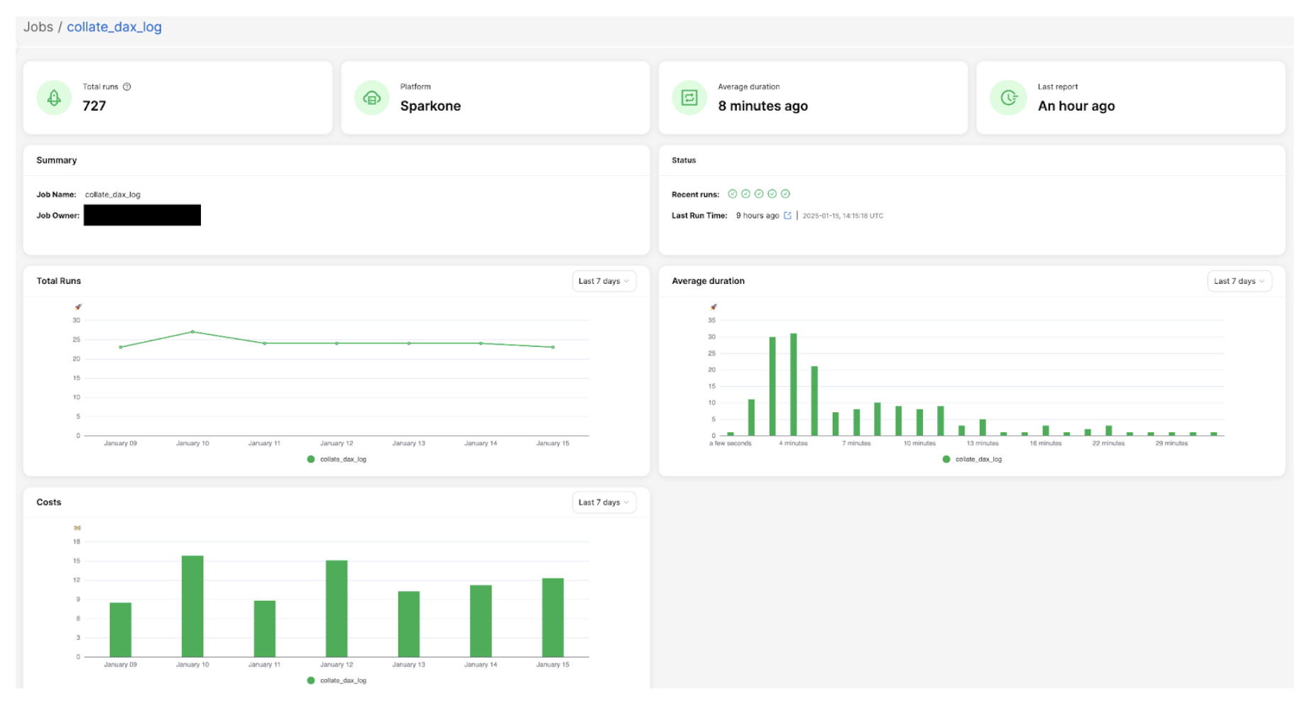
Here is an example of the job overview screen, which displays key summary information: total number of runs, job owner details, performance trends, and cost analysis charts. This comprehensive view provides users with a quick snapshot of their Spark job’s overall health and resource utilisation.
Figure 2: Example of job overview screen
Advanced analytics and insights
One of the key features we’ve implemented in Iris is the ability to perform analytics on historical job runs to capture trends. This feature leverages the power of StarRocks and our data model to provide users with valuable insights and recommendations. Here’s how we’ve implemented it:
Historical run analysis
We’ve created a materialised view that aggregates job run data over the last 30 days. This view likely includes metrics such as count of runs, p95 values for various resource utilisation, etc.
    C/C++
    CREATE MATERIALIZED VIEW job_run_summaries_001
    REFRESH ASYNC EVERY(INTERVAL 1 DAY)
    AS
    select platform,
        job_id,
        count(distinct run_id)                                as count_run,
        ceil(percentile_approx(total_instances, 0.95))        as p95_total_instances,
        ceil(percentile_approx(worker_instances, 0.95))       as p95_worker_instances,
        percentile_approx(job_hour, 0.95)                     as p95_job_hour,
        percentile_approx(machine_hour, 0.95)                 as p95_machine_hour,
        percentile_approx(cpu_hour, 0.95)                     as p95_cpu_hour,
        percentile_approx(worker_gc_hour, 0.95)               as p95_worker_gc_hour,
        ceil(percentile_approx(driver_cpus, 0.95))            as p95_driver_cpus,
        ceil(percentile_approx(worker_cpus, 0.95))            as p95_worker_cpus,
        ceil(percentile_approx(driver_memory_gb, 0.95))       as p95_driver_memory_gb,
        ceil(percentile_approx(worker_memory_gb, 0.95))       as p95_worker_memory_gb,
        percentile_approx(driver_cpu_utilization, 0.95)       as p95_driver_cpu_utilization,
        percentile_approx(worker_cpu_utilization, 0.95)       as p95_worker_cpu_utilization,
        percentile_approx(driver_memory_utilization, 0.95)    as p95_driver_memory_utilization,
        percentile_approx(worker_memory_utilization, 0.95)    as p95_worker_memory_utilization,
        percentile_approx(total_gb_read, 0.95)                as p95_gb_read,
        percentile_approx(total_gb_written, 0.95)             as p95_gb_written,
        percentile_approx(total_memory_gb_spilled, 0.95)      as p95_memory_gb_spilled,
        percentile_approx(disk_spilled_rate, 0.95)            as p95_disk_spilled_rate
    from iris.job_runs
    where report_date >= current_date - interval 30 day
    group by platform, job_id;
Using this aggregated data, we can identify trends in job performance and resource usage over time, such as increasing run times or spikes in resource consumption.
Recommendation API
Based on trend analysis insights, we’ve built a recommendation API that suggests optimizations, such as adjusting resource allocations, identifying potential bottlenecks, or proposing schedule changes to optimise cost and performance.
Frontend integration
The recommendations generated by our API are integrated into the Iris front end. Users can view these recommendations directly in the job overview or details screens, offering actionable insights to improve Spark jobs.
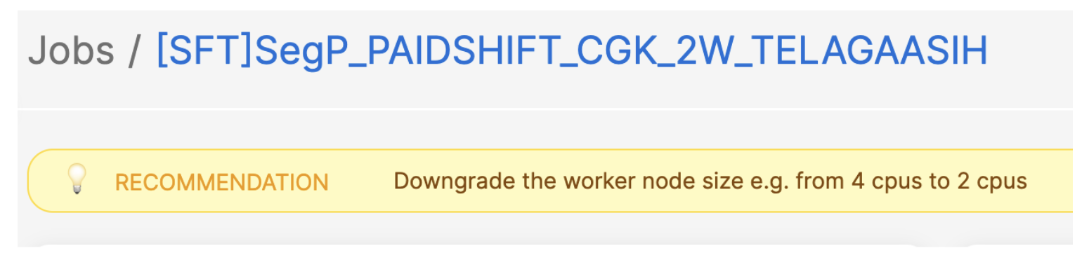
Here is an example: in a job with consistently low resource utilisation (less than 25% over time), our system suggests reducing the worker size by half to optimise costs.
Figure 3. Example of job with low resource utilisation.
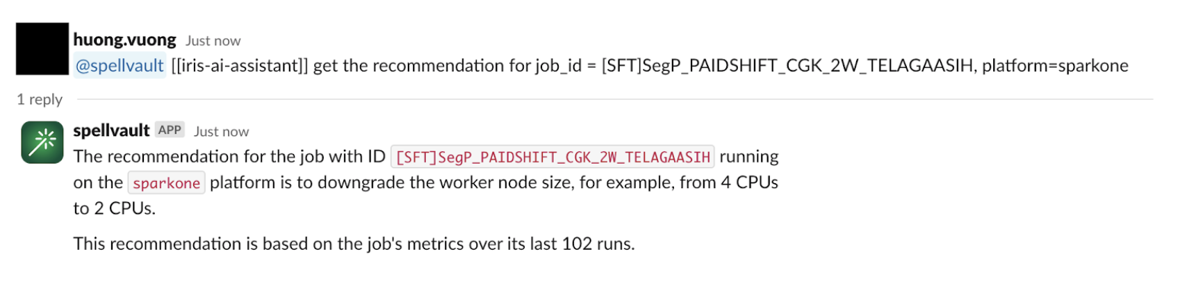
Slackbot integration
To make these insights more accessible, we’ve integrated the recommendation system with a SpellVault app (a GenAI platform at Grab). This allows users to interact with the recommendation system directly from Slack, allowing them to stay informed about job performance and potential optimisations without constantly checking the Iris web interface.
Figure 4. Example of integration with SpellVault.
Migration and adoption
Migration strategy
Fully migrating real-time CPU/Memory charts from Grafana to the new Iris UI
Will deprecate the Grafana dashboard after migration
Retaining Superset for platform metrics and specific BI needs
User onboarding and feedback
Iris deployed within the One DE app, centralising access to data engineering tools. The feedback button in the UI allows users to submit comments easily.
Lessons learned and future roadmap
Lessons learned
Unified data store: Using StarRocks as a single source for both real-time and historical data has significantly improved query performance and streamlined our architecture.
Materialised views: Leveraging StarRocks’ materialised views for pre-aggregations has significantly enhanced query response times, especially for common UI operations.
Dynamic partitioning: Implementing dynamic partitioning has helped in maintaining optimal performance as data volumes grow, automatically managing data retention.
Direct Kafka ingestion: StarRocks’ ability to ingest data directly from Kafka has streamlined our data pipeline, reducing latency and complexity.
Flexible data model: Compared to the previous time-series-focused InfluxDB, the StarRocks relational model enables more complex queries and simplifies metadata handling.
Future roadmap
Enhanced recommendations: Expand the recommendation system to include more in-depth suggestions, such as identifying potential bottlenecks and recommending Spark configurations to add or remove from jobs. These recommendations, aimed at improving runtime and cost performance, will leverage the detailed Spark metrics and event data we’re already collecting.
Advanced analytics: Leverage the comprehensive Spark metrics data to provide deeper insights into job performance and resource utilisation.
Integration expansion: Enhance Iris integration with other internal tools and platforms to increase adoption and ensure a seamless experience across the data engineering ecosystem.
Machine learning integration: Explore the possibility of incorporating machine learning models for predictive analytics on Spark performance.
Scalability improvements: Continue to optimise the system to handle increasing data volumes and user loads as adoption grows.
User experience enhancements: Continuously improve the Iris application’s UI/UX based on user feedback to make it more intuitive and informative.
Conclusion
The journey of building the Iris web application, powered by StarRocks, has been transformative for our Spark observability capabilities at Grab. This evolution was driven by the need for a user-friendly, centralised platform for Spark monitoring and logging.
By leveraging StarRocks’ capabilities, we’ve created a unified interface that seamlessly handles both real-time and historical data. This has allowed us to consolidate previously fragmented tools like Grafana and Superset into a single, cohesive platform. The ability to capture and analyse job metadata and metrics in one place has been crucial, enabling us to implement effective showback/chargeback mechanisms at the job level.
Looking ahead, we’re excited about the potential for more advanced analytics and machine learning-driven insights. The lessons learned from this project will guide our approach to building robust, scalable, and user-friendly data tools at Grab.
Join us
Grab is a leading superapp in Southeast Asia, operating across the deliveries, mobility and digital financial services sectors. Serving over 800 cities in eight Southeast Asian countries, Grab enables millions of people everyday to order food or groceries, send packages, hail a ride or taxi, pay for online purchases or access services such as lending and insurance, all through a single app. Grab was founded in 2012 with the mission to drive Southeast Asia forward by creating economic empowerment for everyone. Grab strives to serve a triple bottom line – we aim to simultaneously deliver financial performance for our shareholders and have a positive social impact, which includes economic empowerment for millions of people in the region, while mitigating our environmental footprint.
Powered by technology and driven by heart, our mission is to drive Southeast Asia forward by creating economic empowerment for everyone. If this mission speaks to you, join our team today!
Well, it’s been another historic year! We’ve watched in awe as the use of real-world generative AI has changed the tech landscape, and while we at the Architecture Blog happily participated, we also made every effort to stay true to our channel’s original scope, and your readership this last year has proven that decision was the right one.
AI/ML carries itself in the top posts this year, but we’re also happy to see that foundational topics like resiliency and cost optimization are still of great interest to our audience.
(By the way, if you were hoping for more AI/ML content, head on over to our sister channel, the AWS Machine Learning Blog!).
Without further ado, here are our top posts from 2024!
In keeping with Let’s Architect! series, we have our first of three favorites for the year. This set of resources helps you apply Well-Architected standards in practice.
As I said, Let’s Architect! has a winning series, and they’ve got a finger on the pulse of the tech world. This post about machine learning showcases some of the most exciting things happening at AWS.
Figure 3. Let’s Architect
If you’re more interested in generative AI, you can also take a look at another post from 2024: Let’s Architect! GenAI
Preparedness is another common theme in this year’s favorites. Michael, John, and Saurabh are well-versed in multi-Region architecture, and they’re here to share some strategies to contain failure impact.
Figure 4. When the application experiences an impairment using S3 resources in the primary Region, it fails over to use an S3 bucket in the secondary Region.
Let’s talk cost optimization. This post about a three-tier architecture that relies on the AWS Free Tier is a must-read for anyone looking for tips to help them avoid unnecessary costs (and that’s everyone).
Figure 5. Example of a three-tier architecture on AWS
As usual, Haleh & team are pros at making sure the Well-Architected Framework is current and relevant. Take a look at the enhanced and expanded guidance in all six pillars.
One more winning post from Luca, Federica, Vittorio, and Zamira! This collection of developer resources includes new ideas in AWS Lambda, Amazon Q Developer, and Amazon DynamoDB.
Frugality AND Well-Architected? What a winning combo! This post, inspired by the 2023 re:Invent keynote, outlines the seven laws of Frugal Architecture.
And finally, our number one post of the year! Amit and Luiz showcase a customer solution with real-world applications that builds on the guidelines of other posts in this list! Well done!
Figure 10. The Pilot Light scenario for a 3-tier application that has application servers and a database deployed in two Regions
Thank you!
As always, thanks to our contributors for their dedication and desire to share, and to you, our readers! We would be nothing with you. Literally.
For other top post lists, see our Top 10 and Top 5 posts from previous years.
A data-driven approach empowers businesses to make informed decisions based on accurate predictions and forecasts, leading to improved operational efficiency and resource optimization. Machine learning (ML) systems have the remarkable ability to continuously learn and adapt, improving their performance over time as they are exposed to more data. This self-learning capability ensures that organizations can stay ahead of the curve, responding dynamically to changing market conditions and customer preferences, ultimately driving innovation and enhancing competitiveness.
By leveraging the power of machine learning on AWS, businesses can unlock benefits that enhance efficiency, improve decision-making, and foster growth.
In this session, see how organizations with constrained resources (budgets, skill gaps, time) can jump start their data-driven journey with advanced analytics and ML capabilities. Learn AWS Working Backwards best practices to drive forward data-related projects that address tangible business value. Then dive into AWS analytics and AI/ML capabilities that simplify and expedite data pipeline delivery and business value from ML workloads. Hear about low-code no-code (LCNC) AWS services within the context of a complete data pipeline architecture.
As artificial intelligence (AI) continues to revolutionize industries, the ability to operationalize and scale ML models has become a critical challenge. This session introduces the concept of MLOps, a discipline that builds upon and extends the widely adopted DevOps practices prevalent in software development. By applying MLOps principles, organizations can streamline the process of building, training, and deploying ML models, ensuring efficient and reliable model lifecycle management. By mastering MLOps, organizations can bridge the gap between AI development and operations, enabling them to unlock the full potential of their ML initiatives.
To power generative AI applications while keeping costs under control, AWS designs and builds machine learning accelerators like AWS Trainium and AWS Inferentia. This session introduces purpose-built ML hardware for model training and inference, and shows how Amazon and AWS customers take advantage of those solutions to optimize costs and reduce latency.
You can learn from practical examples showing the impact of those solutions and explanations about how these chips work. ML accelerators are not only beneficial for generative AI workloads; they can also be applied to other use cases, including representation learning, recommender systems, or any scenario with deep neural network models.
Figure 3. Discover the technology that powers our AI services
How our customers are implementing machine learning on AWS
The following resources drill down into the ML infrastructure that’s used to train large models at Pinterest and the experimentation framework built by Booking.com.
The Pinterest video discusses the strategy to create an ML development environment, orchestrate training jobs, ingest data into the training loop, and accelerate the training speed. You can also learn about the advantages derived from containers in the context of ML and how Pinterest decided to set up the entire ML lifecycle, including distributed model training.
The second resource covers how Booking.com accelerated the experimentation process by leveraging Amazon SageMaker for data analysis, model training, and online experimentation. This resulted in shorter development times for their ranking models and increased speed for the data science teams.
Amazon SageMaker Immersion Day helps customers and partners provide end-to-end understanding of building ML use cases. From feature engineering to understanding various built-in algorithms, with a focus on training, tuning, and deploying the ML model in a production-like scenario, this workshop guides you to bring your own model to perform lift-and-shift from on-premises to the Amazon SageMaker platform. It further demonstrates more advanced concepts like model debugging, model monitoring, and AutoML.
Figure 5. Train, tune and deploy your workload using Amazon SageMaker
See you next time!
Thanks for reading! With this post, introduced you to the art of possibility on using AWS machine learning services. In the next blog, we will talk about cloud migrations.
To revisit any of our previous posts or explore the entire series, visit the Let’s Architect! page.
In the domain of data processing, data analysts run their ad hoc queries on the data lake. The lake serves as an interface between our analytics and production environment, preventing downstream queries from impacting upstream data ingestion pipelines. To ensure efficient data processing in the data lake, choosing appropriate storage formats is crucial.
The vanilla data lake solution is built on top of cloud object storage with Hive metastore, where data files are written in Parquet format. Although this setup is optimised for scalable analytics query patterns, it struggles to handle frequent updates to the data due to two reasons:
The Hive table format requires us to rewrite the Parquet files with the latest data. For instance, to update one record in a Hive unpartitioned table, we would need to read all the data, update the record, and write back the entire data set.
Writing Parquet files is expensive due to the overhead of organising the data to a compressed columnar format, which is more complex than a row format.
The issue is further exacerbated by the scheduled downstream transformations. These necessary steps, which clean and process the data for use, increase the latency because the total delay now includes the combined scheduled intervals of these processing jobs.
Fortunately, the introduction of the Hudi format, which supports fast writes by allowing Avro and Parquet files to co-exist on a Merge On Read (MOR) table, opens up the possibility of having a data lake with minimal data latency. The concept of a commit timeline further allows data to be served with Atomicity, Consistency, Isolation, and Durability (ACID) guarantees.
We employ different sets of configurations for the different characteristics of our input sources:
High or low throughput. A high-throughput source refers to one that has a high level of activity. One example of this can be our stream of booking events generated from each customer transaction. On the other hand, a low-throughput source would be one that has a relative low level of activity. An example of this can be transaction events generated from reconciliation happening on a nightly basis.
Kafka (unbounded) or Relational Database Sources (bounded). Our sinks have sources that can be broadly categorised into unbounded and bounded sources. Unbounded sources are usually related to transaction events materialised as Kafka topics, representing user-generated events as they interact with the Grab superapp. Bounded sources usually refer to Relational Database (RDS) sources, whose size is bound to storage provisioned.
The following sections will delve into the differences between each source and our corresponding configurations optimised for them.
High throughput source
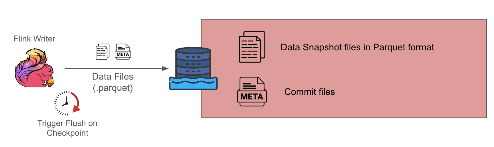
For our data sources with high throughput, we have chosen to write the files in MOR format since the writing of files in Avro format allows for fast writes to meet our latency requirements.
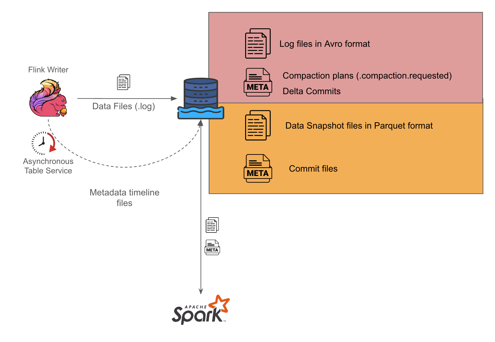
Figure 1 Architecture for MOR tables
As seen in Figure 1, we use Flink to perform the stream processing and write out log files in Avro format in our setup. We then set up a separate Spark writer which periodically converts the Avro files into Parquet format in the Hudi compaction process.
We have further simplified the coordination between the Flink and Spark writers by enabling asynchronous services on the Flink writer so it can generate the compaction plans for Spark writers to act on. During the Spark job runs, it checks for available compaction plans and acts on them, placing the burden of orchestrating the writes solely on the Flink writer. This approach could help minimise potential concurrency problems that might otherwise arise, as there would be a single actor
orchestrating the associated Hudi table services.
Low throughput source
Figure 2 Architecture for COW tables
For low throughput sources, we gravitate towards the choice of Copy On Write (COW) tables given the simplicity of its design, since it only involves one component, which is the Flink writer. The downside is that it has higher data latency because this setup only generates Parquet format data snapshots at each checkpoint interval, which is typically about 10-15 minutes.
Connecting to our Kafka (unbounded) data source
Grab uses Protobuf as our central data format in Kafka, ensuring schema evolution compatibility. However, the derivation of the schema of these topics still requires some transformation to make it compatible with Hudi’s accepted schema. Some of these transformations include ensuring that Avro record fields do not contain just a single array field, and handling logical decimal schemas to transform them to fixed byte schema for Spark compatibility.
Given the unbounded nature of the source, we decided to partition it by Kafka event time up to the hour level. This ensured that our Hudi operations would be faster. Parquet file writes would be faster since they would only affect files within the same partition, and each Parquet file within the same event time partition would have a bounded size given the monotonically increasing nature of Kafka event time.
By partitioning tables by Kafka event time, we can further optimise compaction planning operations, since the amount of file lookups required is now reduced with the use of BoundedPartitionAwareCompactionStrategy. Only log files in recent partitions would be selected for compaction and the job manager need not list every partition to figure out which log files to select for compaction during the planning phase anymore.
Connecting to our RDS (bounded) data source
For our RDS, we decided to use the Flink Change Data Capture (CDC) connectors by Veverica to obtain the binlog streams. The RDS would then treat the Flink writer as a replication server and start streaming its binlog data to it for each MySQL change. The Flink CDC connector presents the data as a Kafka Connect (KC) Source record, since it uses the Debezium connector under the hood. It is then a straightforward task to deserialise these records and transform them into Hudi records, since
the Avro schema and associated data changes are already captured within the KC source record.
The obtained binlog timestamp is also emitted as a metric during consumption for us to monitor the observed data latency at the point of ingestion.
Optimising for these sources involves two phases:
First, assigning more resources for the cold start incremental snapshot process where Flink takes a snapshot of the current data state in the RDS and loads the Hudi table with that snapshot. This phase is usually resource-heavy as there are a lot of file writes and data ingested during this process.
Once the snapshotting is completed, Flink would then start to process the binlog stream and the observed throughput would drop to a level similar to the DB write throughput. The resources required by the Flink writer at this stage would be much lower than in the snapshot phase.
Indexing for Hudi tables
Indexing is important for upserting Hudi tables when the writing engine performs updates, allowing it to efficiently locate the file groups of the data to be updated.
As of version 0.14, the Flink engine only supports Bucket Index or Flink State Index. Bucket Index performs indexing of the file record by hashing the record key and matching it to a specific bucket of files indicated by the naming convention of the written data files. Flink State Index on the other hand stores the index map of record keys to files in memory.
Given that our tables include unbounded Kafka sources, there is a possibility for our state indexes to grow indefinitely. Furthermore, the requirement of state preservation for Flink State Index across version deployments and configuration updates adds complexity to the overall solution.
Thus, we opted for the simple Bucket Index for its simplicity and the fact that our Hudi table size per partition does not change drastically across the week. However, this comes with a limitation whereby the number of buckets cannot be updated easily and imposes a parallelism limit at which our Flink pipelines can scale. Thus, as traffic grows organically, we would find ourselves in a situation whereby our configuration grows obsolete and cannot handle the increased load.
To resolve this going forward, using consistent hashing for the Bucket Index would be something to explore to optimise our Parquet file sizes and allow the number of buckets to grow seamlessly as traffic grows.
Impact
Fresh business metrics
Post creation of our Hudi Data Ingestion solution, we have enabled various users such as our data analysts to perform ad hoc queries much more easily on data that has lower latency. Furthermore, Hudi tables can be seamlessly joined with Hive tables in Trino for additional context. This enabled the construction of operational dashboards reflecting fresh business metrics to our various operators, empowering them with the necessary information to quickly respond to any abnormalities (such as high-demand events like F1 or seasonal holidays).
Quicker fraud detection
Another significant user of our solution is our fraud detection analysts. This enabled them to rapidly access fresh transaction events and analyse them for fraudulent patterns, particularly during the emergence of a new attack pattern that hadn’t been detected by their rules engine. Our solution also allowed them to perform multiple ad hoc queries that involve lookbacks of various days’ worth of data without impacting our production RDS and Kafka clusters by using the data lake as the data interface, reducing the data latency to the minute level and, in turn, empowering them to respond more quickly to attacks.
What’s next?
As the landscape of data storage solutions evolves rapidly, we are eager to test and integrate new features like Record Level Indexing and the creation of Pre Join tables. This evolution extends beyond the Hudi community to other table formats such as IceBerg and DeltaLake. We remain ready to adapt ourselves to these changes and incorporate the advantages of each format into our data lake within Grab.
Grab is the leading superapp platform in Southeast Asia, providing everyday services that matter to consumers. More than just a ride-hailing and food delivery app, Grab offers a wide range of on-demand services in the region, including mobility, food, package and grocery delivery services, mobile payments, and financial services across 428 cities in eight countries.
Powered by technology and driven by heart, our mission is to drive Southeast Asia forward by creating economic empowerment for everyone. If this mission speaks to you, join our team today!
As businesses race to digitally transform, the challenge is to cope with the amount of data, and the value of that data diminishes over time. The challenge is to analyze, learn, and infer from real-time data to predict future states, as well as to detect anomalies and get accurate results. In this blog post, we’ll explain the architecture for a solution that can achieve real-time inference on streaming data. We’ll also cover the integration of Amazon Kinesis Data Analytics (KDA) with Apache Flink to asynchronously invoke any underlying services (or databases).
Managed real-time in-stream data inference is quite a mouthful; let’s break it up:
In-stream data refers to the capability of processing a data stream that collects, processes, and analyzes data.
Real-time inference refers to the ability to use data from the feed to project future state for the underlying data.
Consider a streaming application that captures credit card transactions along with the other parameters (such as source IP to capture the geographic details of the transaction as well as the amount). This data can then be used to be used to infer fraudulent transactions instantaneously. Compare that to a traditional batch-oriented approach that identifies fraudulent transactions at the end of every business day and generates a report when it’s too late, after bad actors have already committed fraud.
Architecture overview
In this post, we discuss how you can use Amazon Kinesis Data Analytics for Apache Flink (KDA), Amazon SageMaker, Apache Flink, and Amazon API Gateway to address the challenges such as real-time fraud detection on a stream of credit card transaction data. We explore how to build a managed, reliable, scalable, and highly available streaming architecture based on managed services that substantially reduce the operational overhead compared to a self-managed environment. Our particular focus is on how to prepare and run Flink applications with KDA for Apache Flink applications.
The following diagram illustrates this architecture:
In above architecture, data is ingested in AWS Kinesis Data Streams (KDS) using Amazon Kinesis Producer Library (KPL), and you can use any ingestion patterns supported by KDS. KDS then streams the data to an Apache Flink-based KDA application. KDA manages the required infrastructure for Flink, scales the application in response to changing traffic patterns, and automatically recovers from underlying failures. The Flink application is configured to call an API Gateway endpoint using Asynchronous I/O. Residing behind the API Gateway is an AWS SageMaker endpoint, but any endpoints can be used based on your data enrichment needs. Flink distributes the data across one or more stream partitions, and user-defined operators can transform the data stream.
Let’s talk about some of the key pieces of this architecture.
What is Apache Flink?
Apache Flink is an open source distributed processing framework that is tailored to stateful computations over unbounded and bounded datasets. The architecture uses KDA with Apache Flink to run in-stream analytics and uses Asynchronous I/O operator to interact with external systems.
KDA and Apache Flink
KDA for Apache Flink is a fully managed AWS service that enables you to use an Apache Flink application to process streaming data. With KDA for Apache Flink, you can use Java or Scala to process and analyze streaming data. The service enables you to author and run code against streaming sources. KDA provides the underlying infrastructure for your Flink applications. It handles core capabilities like provisioning compute resources, parallel computation, automatic scaling, and application backups (implemented as checkpoints and snapshots).
Flink Asynchronous I/O Operator
Flink’s Asynchronous I/O operator allows you to use asynchronous request clients for external systems to enrich stream events or perform computation. Asynchronous interaction with the external system means that a single parallel function instance can handle multiple requests and receive the responses concurrently. In most cases this leads to higher streaming throughput. Asynchronous I/O API integrates well with data streams, and handles order, event time, fault tolerance, etc. You can configure this operator to call external sources like databases and APIs. The architecture pattern explained in this post is configured to call API Gateway integrated with SageMaker endpoints.
Please refer code at kda-flink-ml, a sample Flink application with implementation of Asynchronous I/O operator to call an external Sagemaker endpoint via API Gateway. Below is the snippet of code of StreamingJob.java from sample Flink application.
The operator code above requires following inputs:
An input data stream
An implementation of AsyncFunction that dispatches the requests to the external system
Timeout, which defines how long an asynchronous request may take before it considered failed
Capacity, which defines how many asynchronous requests may be in progress at the same time
How Amazon SageMaker fits into this puzzle
In our architecture we are proposing a SageMaker endpoint for inferencing that is invoked via API Gateway, which can detect fraudulent transactions.
Amazon SageMaker is a fully managed service that provides every developer and data scientist with the ability to build, train, and deploy machine learning (ML) models quickly. SageMaker removes the heavy lifting from each step of the machine learning process to make it easier to build and develop high quality models. You can use these trained models in an ingestion pipeline to make real-time inferences.
You can set up persistent endpoints to get predictions from your models that are deployed on SageMaker hosting services. For an overview on deploying a single model or multiple models with SageMaker hosting services, see Deploy a Model on SageMaker Hosting Services.
Ready for a test drive
To help you get started, we would like to introduce an AWS Solution: AWS Streaming Data Solution for Amazon Kinesis (Option 4) that is available as a single-click cloud formation template to assist you in quickly provisioning resources to get your real-time in-stream inference pipeline up and running in a few minutes. In this solution we leverage AWS Lambda, but that can be switched with a SageMaker endpoint to achieve the architecture discussed earlier in this post. You can also leverage the pre-built AWS Solutions Construct, which implements an Amazon API Gateway connected to an Amazon SageMaker endpoint pattern that can replace AWS Lambda in the below solution. See the implementation guide for this solution.
The following diagram illustrates the architecture for the solution:
Conclusion
In this post we explained the architecture to build a managed, reliable, scalable, and highly available application that is capable of real-time inferencing on a data stream. The architecture was built using KDS, KDA for Apache Flink, Apache Flink, and Amazon SageMaker. The architecture also illustrates how you can use managed services so that you don’t need to spend time provisioning, configuring, and managing the underlying infrastructure. Instead, you can spend your time creating insights and inference from your data.
We also talked about the AWS Streaming Data Solution for Amazon Kinesis, which is an AWS vetted solution that provides implementations for applications you can automatically deploy directly into your AWS account. The solution automatically configures the AWS services necessary to easily capture, store, process, and infer from streaming data.
One of the keys to identifying timely and impactful actions is having enough raw material to work with. However, this up-to-date information typically lives in the databases that sit behind several different applications. One of the first steps to finding data-driven insights is gathering that information into a single store that an analyst can use without interfering with those applications.
For years, reporting environments have relied on a data warehouse stored in a single, separate relational database management system (RDBMS). But now, due to the growing use of Software as a service (SaaS) applications and NoSQL database options, data may be stored outside the data center and in formats other than tables of rows and columns. It’s increasingly difficult to access the data these applications maintain, and a data warehouse may not be flexible enough to house the gathered information.
For these reasons, reporting teams are building data lakes, and those responsible for using data analytics at universities and colleges are no different. However, it can be challenging to know exactly how to start building this expanded data repository so it can be ready to use quickly and still expandable as future requirements are uncovered. Helping higher education institutions address these challenges is the topic of this post.
About Maryville University
Maryville University is a nationally recognized private institution located in St. Louis, Missouri, and was recently named the second fastest growing private university by The Chronicle of Higher Education. Even with its enrollment growth, the university is committed to a highly personalized education for each student, which requires reliable data that is readily available to multiple departments. University leaders want to offer the right help at the right time to students who may be having difficulty completing the first semester of their course of study. To get started, the data experts in the Office of Strategic Information and members of the IT Department needed to create a data environment to identify students needing assistance.
Critical data sources
Like most universities, Maryville’s student-related data centers around two significant sources: the student information system (SIS), which houses student profiles, course completion, and financial aid information; and the learning management system (LMS) in which students review course materials, complete assignments, and engage in online discussions with faculty and fellow students.
The first of these, the SIS, stores its data in an on-premises relational database, and for several years, a significant subset of its contents had been incorporated into the university’s data warehouse. The LMS, however, contains data that the team had not tried to bring into their data warehouse. Moreover, that data is managed by a SaaS application from Instructure, called “Canvas,” and is not directly accessible for traditional extract, transform, and load (ETL) processing. The team recognized they needed a new approach and began down the path of creating a data lake in AWS to support their analysis goals.
Getting started on the data lake
The first step the team took in building their data lake made use of an open source solution that Harvard’s IT department developed. The solution, comprised of AWS Lambda functions and Amazon Simple Storage Service (S3) buckets, is deployed using AWS CloudFormation. It enables any university that uses Canvas for their LMS to implement a solution that moves LMS data into an S3 data lake on a daily basis. The following diagram illustrates this portion of Maryville’s data lake architecture:
Diagram 1: The data lake for the Learning Management System data
The AWS Lambda functions invoke the LMS REST API on a daily schedule resulting in Maryville’s data, which has been previously unloaded and compressed by Canvas, to be securely stored into S3 objects. AWS Glue tables are defined to provide access to these S3 objects. Amazon Simple Notification Service (SNS) informs stakeholders the status of the data loads.
Expanding the data lake
The next step was deciding how to copy the SIS data into S3. The team decided to use the AWS Database Migration Service (DMS) to create daily snapshots of more than 2,500 tables from this database. DMS uses a source endpoint for secure access to the on-premises database instance over VPN. A target endpoint determines the specific S3 bucket into which the data should be written. A migration task defines which tables to copy from the source database along with other migration options. Finally, a replication instance, a fully managed virtual machine, runs the migration task to copy the data. With this configuration in place, the data lake architecture for SIS data looks like this:
Diagram 2: Migrating data from the Student Information System
Handling sensitive data
In building a data lake you have several options for handling sensitive data including:
Leaving it behind in the source system and avoid copying it through the data replication process
Copying it into the data lake, but taking precautions to ensure that access to it is limited to authorized staff
Copying it into the data lake, but applying processes to eliminate, mask, or otherwise obfuscate the data before it is made accessible to analysts and data scientists
The Maryville team decided to take the first of these approaches. Building the data lake gave them a natural opportunity to assess where this data was stored in the source system and then make changes to the source database itself to limit the number of highly sensitive data fields.
Validating the data lake
With these steps completed, the team turned to the final task, which was to validate the data lake. For this process they chose to make use of Amazon Athena, AWS Glue, and Amazon Redshift. AWS Glue provided multiple capabilities including metadata extraction, ETL, and data orchestration. Metadata extraction, completed by Glue crawlers, quickly converted the information that DMS wrote to S3 into metadata defined in the Glue data catalog. This enabled the data in S3 to be accessed using standard SQL statements interactively in Athena. Without the added cost and complexity of a database, Maryville’s data analyst was able to confirm that the data loads were completing successfully. He was also able to resolve specific issues encountered on particular tables. The SQL queries, written in Athena, could later be converted to ETL jobs in AWS Glue, where they could be triggered on a schedule to create additional data in S3. Athena and Glue enabled the ETL that was needed to transform the raw data delivered to S3 into prepared datasets necessary for existing dashboards.
Once curated datasets were created and stored in S3, the data was loaded into an AWS Redshift data warehouse, which supported direct access by tools outside of AWS using ODBC/JDBC drivers. This capability enabled Maryville’s team to further validate the data by attaching the data in Redshift to existing dashboards that were running in Maryville’s own data center. Redshift’s stored procedure language allowed the team to port some key ETL logic so that the engineering of these datasets could follow a process similar to approaches used in Maryville’s on-premises data warehouse environment.
Conclusion
The overall data lake/data warehouse architecture that the Maryville team constructed currently looks like this:
Diagram 3: The complete architecture
Through this approach, Maryville’s two-person team has moved key data into position for use in a variety of workloads. The data in S3 is now readily accessible for ad hoc interactive SQL workloads in Athena, ETL jobs in Glue, and ultimately for machine learning workloads running in EC2, Lambda or Amazon Sagemaker. In addition, the S3 storage layer is easy to expand without interrupting prior workloads. At the time of this writing, the Maryville team is both beginning to use this environment for machine learning models described earlier as well as adding other data sources into the S3 layer.
Acknowledgements
The solution described in this post resulted from the collaborative effort of Christine McQuie, Data Engineer, and Josh Tepen, Cloud Engineer, at Maryville University, with guidance from Travis Berkley and Craig Jordan, AWS Solutions Architects.
The collective thoughts of the interwebz
Manage Consent
To provide the best experiences, we use technologies like cookies to store and/or access device information. Consenting to these technologies will allow us to process data such as browsing behavior or unique IDs on this site. Not consenting or withdrawing consent, may adversely affect certain features and functions.
Functional
Always active
The technical storage or access is strictly necessary for the legitimate purpose of enabling the use of a specific service explicitly requested by the subscriber or user, or for the sole purpose of carrying out the transmission of a communication over an electronic communications network.
Preferences
The technical storage or access is necessary for the legitimate purpose of storing preferences that are not requested by the subscriber or user.
Statistics
The technical storage or access that is used exclusively for statistical purposes.The technical storage or access that is used exclusively for anonymous statistical purposes. Without a subpoena, voluntary compliance on the part of your Internet Service Provider, or additional records from a third party, information stored or retrieved for this purpose alone cannot usually be used to identify you.
Marketing
The technical storage or access is required to create user profiles to send advertising, or to track the user on a website or across several websites for similar marketing purposes.