In September 2025, a thread popped up in our internal engineering chat room asking, “Which part of our stack would be responsible for sending ErrCode=ENHANCE_YOUR_CALM to an HTTP/2 client?” Two internal microservices were experiencing a critical error preventing their communication and the team needed a timely answer.
In this blog post, we describe the background to well-known HTTP/2 attacks that trigger Cloudflare defences, which close connections. We then document an easy-to-make mistake using Go’s standard library that can cause clients to send PING flood attacks and how you can avoid it.
HTTP/2 is powerful – but it can be easy to misuse
HTTP/2 defines a binary wire format for encoding HTTP semantics. Request and response messages are encoded as a series of HEADERS and DATA frames, each associated with a logical stream, sent over a TCP connection using TLS. There are also control frames that relate to the management of streams or the connection as a whole. For example, SETTINGS frames advertise properties of an endpoint, WINDOW_UPDATE frames provide flow control credit to a peer so that it can send data, RST_STREAM can be used to cancel or reject a request or response, while GOAWAY can be used to signal graceful or immediate connection closure.
HTTP/2 provides many powerful features that have legitimate uses. However, with great power comes responsibility and opportunity for accidental or intentional misuse. The specification details a number of denial-of-service considerations. Implementations are advised to harden themselves: “An endpoint that doesn’t monitor use of these features exposes itself to a risk of denial of service. Implementations SHOULD track the use of these features and set limits on their use.”
Cloudflare implements many different HTTP/2 defenses, developed over years in order to protect our systems and our customers. Some notable examples include mitigations added in 2019 to address “Netflix vulnerabilities” and in 2023 to mitigate Rapid Reset and similar style attacks.
When Cloudflare detects that HTTP/2 client behaviour is likely malicious, we close the connection using the GOAWAY frame and include the error code ENHANCE_YOUR_CALM.
One of the well-known and common attacks is CVE-2019-9512, aka PING flood: “The attacker sends continual pings to an HTTP/2 peer, causing the peer to build an internal queue of responses. Depending on how efficiently this data is queued, this can consume excess CPU, memory, or both.” Sending a PING frame causes the peer to respond with a PING acknowledgement (indicated by an ACK flag). This allows for checking the liveness of the HTTP connection, along with measuring the layer 7 round-trip time – both useful things. The requirement to acknowledge a PING, however, provides the potential attack vector since it generates work for the peer.
A client that PINGs the Cloudflare edge too frequently will trigger our CVE-2019-9512 mitigations, causing us to close the connection. Shortly after we launched support for gRPC in 2020, we encountered interoperability issues with some gRPC clients that sent many PINGs as part of a performance optimization for window tuning. We also discovered that the Rust Hyper crate had a feature called Adaptive Window that emulated the design and triggered a similar problem until Hyper made a fix.
Solving a microservice miscommunication mystery
When that thread popped up asking which part of our stack was responsible for sending the ENHANCE_YOUR_CALM error code, it was regarding a client communicating over HTTP/2 between two internal microservices.
We suspected that this was an HTTP/2 mitigation issue and confirmed it was a PING flood mitigation in our logs. But taking a step back, you may wonder why two internal microservices are communicating over the Cloudflare edge at all, and therefore hitting our mitigations. In this case, communicating over the edge provides us with several advantages:
We get to dogfood our edge infrastructure and discover issues like this!
We can use Cloudflare Access for authentication. This allows our microservices to be accessed securely by both other services (using service tokens) and engineers (which is invaluable for debugging).
Internal services that are written with Cloudflare Workers can easily communicate with services that are accessible at the edge.
The question remained: Why was this client behaving this way? We traded some ideas as we attempted to get to the bottom of the issue.
The client had a configuration that would indicate that it didn’t need to PING very frequently:
However, in situations like this it is generally a good idea to establish ground truth about what is really happening “on the wire.” For instance, grabbing a packet capture that can be dissected and explored in Wireshark can provide unequivocal evidence of precisely what was sent over the network. The next best option is detailed/trace logging at the sender or receiver, although sometimes logging can be misleading, so caveat emptor.
In our particular case, it was simpler to use logging with GODEBUG=http2debug=2. We built a simplified minimal reproduction of the client that triggered the error, helping to eliminate other potential variables. We did some group log analysis, combined with diving into some of the Go standard library code to understand what it was really doing. Issac Asimov is commonly credited with the quote “The most exciting phrase to hear in science, the one that heralds new discoveries, is not ‘Eureka!’ but ‘That’s funny…'” and sure enough, within the hour someone declared–
the funny part I see is this:
2025/09/02 17:33:18 http2: Framer 0x14000624540: wrote RST_STREAM stream=9 len=4 ErrCode=CANCEL
2025/09/02 17:33:18 http2: Framer 0x14000624540: wrote PING len=8 ping="j\xe7\xd6R\xdaw\xf8+"
every ping seems to be preceded by a RST_STREAM
Observant readers will recall the earlier mention of Rapid Reset. However, our logs clearly indicated ENHANCE_YOUR_CALM being triggered due to the PING flood. A bit of searching landed us on this mailing list thread and the comment “Sending a PING frame along with an RST_STREAM allows a client to distinguish between an unresponsive server and a slow response.” That seemed quite relevant. We also found a change that was committed related to this topic. This partly answered why there were so many PINGs, but it also raised a new question: Why so many stream resets?
So we went back to the logs and built up a little more context about the interaction:
2025/09/02 17:33:18 http2: Transport received DATA flags=END_STREAM stream=47 len=0 data=""
2025/09/02 17:33:18 http2: Framer 0x14000624540: wrote RST_STREAM stream=47 len=4 ErrCode=CANCEL
2025/09/02 17:33:18 http2: Framer 0x14000624540: wrote PING len=8 ping="\x97W\x02\xfa>\xa8\xabi"
The interesting thing here is that the server had sent a DATA frame with the END_STREAM flag set. Per the HTTP/2 stream state machine, the stream should have transitioned to closed when a frame with END_STREAM was processed. The client doesn’t need to do anything in this state – sending a RST_STREAM is entirely unnecessary.
A little more digging and noodling and an engineer proclaimed:
I noticed that the reset+ping only happens when you call resp.Body.Close()
I believe Go’s HTTP library doesn’t actually read the response body automatically, but keeps the stream open for you to use until you call resp.Body.Close(), which you can do at any point you like.
The hilarious thing in our example was that there wasn’t actually any HTTP body to read. From the earlier example: received DATA flags=END_STREAM stream=47 len=0 data="".
Science and engineering are at times weird and counterintuitive. We decided to tweak our client to read the (absent) body via io.Copy(io.Discard, resp.Body) before closing it.
Sure enough, this immediately stopped the client sending both a useless RST_STREAM and, by association, a PING frame.
Mystery solved?
To prove we had fixed the root cause, the production client was updated with a similar fix. A few hours later, all the ENHANCE_YOUR_CALM closures were eliminated.
Reading bodies in Go can be unintuitive
It’s worth noting that in some situations, ensuring the response body is always read can sometimes be unintuitive in Go. For example, at first glance it appears that the response body will always be read in the following example:
However, json.Decoder stops reading as soon as it finds a complete JSON document or errors. If the response body contains multiple JSON documents or invalid JSON, then the entire response body may still not be read.
Therefore, in our clients, we’ve started replacing defer response.Body.Close() with the following pattern to ensure that response bodies are always fully read:
Actions to take if you encounter ENHANCE_YOUR_CALM
HTTP/2 is a protocol with several features. Many implementations have implemented hardening to protect themselves from misuse of features, which can trigger a connection to be closed. The recommended error code for closing connections in such conditions is ENHANCE_YOUR_CALM. There are numerous HTTP/2 implementations and APIs, which may drive the use of HTTP/2 features in unexpected ways that could appear like attacks.
If you have an HTTP/2 client that encounters closures with ENHANCE_YOUR_CALM, we recommend that you try to establish ground truth with packet captures (including TLS decryption keys via mechanisms like SSLKEYLOGFILE) and/or detailed trace logging. Look for patterns of frequent or repeated frames that might be similar to malicious traffic. Adjusting your client may help avoid it getting misclassified as an attacker.
If you use Go, we recommend always reading HTTP/2 response bodies (even if empty) in order to avoid sending unnecessary RST_STREAM and PING frames. This is especially important if you use a single connection for multiple requests, which can cause a high frequency of these frames.
This was also a great reminder of the advantages of dogfooding our own products within our internal services. When we run into issues like this one, our learnings can benefit our customers with similar setups.
Every second, 84 million HTTP requests are hitting Cloudflare across our fleet of data centers in 330 cities. It means that even the rarest of bugs can show up frequently. In fact, it was our scale that recently led us to discover a bug in Go’s arm64 compiler which causes a race condition in the generated code.
This post breaks down how we first encountered the bug, investigated it, and ultimately drove to the root cause.
Investigating a strange panic
We run a service in our network which configures the kernel to handle traffic for some products like Magic Transit and Magic WAN. Our monitoring watches this closely, and it started to observe very sporadic panics on arm64 machines.
We first saw one with a fatal error stating that traceback did not unwind completely. That error suggests that invariants were violated when traversing the stack, likely because of stack corruption. After a brief investigation we decided that it was probably rare stack memory corruption. This was a largely idle control plane service where unplanned restarts have negligible impact, and so we felt that following up was not a priority unless it kept happening.
And then it kept happening.
Coredumps per hour
When we first saw this bug we saw that the fatal errors correlated with recovered panics. These were caused by some old code which used panic/recover as error handling.
At this point, our theory was:
All of the fatal panics happen within stack unwinding.
We correlated an increased volume of recovered panics with these fatal panics.
Recovering a panic unwinds goroutine stacks to call deferred functions.
A related Go issue (#73259) reported an arm64 stack unwinding crash.
Let’s stop using panic/recover for error handling and wait out the upstream fix?
So we did that and watched as fatal panics stopped occurring as the release rolled out. Fatal panics gone, our theoretical mitigation seemed to work, and this was no longer our problem. We subscribed to the upstream issue so we could update when it was resolved and put it out of our minds.
But, this turned out to be a much stranger bug than expected. Putting it out of our minds was premature as the same class of fatal panics came back at a much higher rate. A month later, we were seeing up to 30 daily fatal panics with no real discernible cause; while that might account for only one machine a day in less than 10% of our data centers, we found it concerning that we didn’t understand the cause. The first thing we checked was the number of recovered panics, to match our previous pattern, but there were none. More interestingly, we could not correlate this increased rate of fatal panics with anything. A release? Infrastructure changes? The position of Mars?
At this point we felt like we needed to dive deeper to better understand the root cause. Pattern matching and hoping was clearly insufficient.
We saw two classes of this bug — a crash while accessing invalid memory and an explicitly checked fatal error.
Now we could observe some clear patterns. Both errors occur when unwinding the stack in (*unwinder).next. In one case we saw an intentionalfatal error as the runtime identified that unwinding could not complete and the stack was in a bad state. In the other case there was a direct memory access error that happened while trying to unwind the stack. The segfault was discussed in the GitHub issue and a Go engineer identified it as dereference of a go scheduler struct, m, whenunwinding.
A review of Go scheduler structs
Go uses a lightweight userspace scheduler to manage concurrency. Many goroutines are scheduled on a smaller number of kernel threads – this is often referred to as M:N scheduling. Any individual goroutine can be scheduled on any kernel thread. The scheduler has three core types – g (the goroutine), m (the kernel thread, or “machine”), and p (the physical execution context, or “processor”). For a goroutine to be scheduled a free m must acquire a free p, which will execute a g. Each g contains a field for its m if it is currently running, otherwise it will be nil. This is all the context needed for this post but the go runtime docs explore this more comprehensively.
At this point we can start to make inferences on what’s happening: the program crashes because we try to unwind a goroutine stack which is invalid. In the first backtrace, if a return address is null, we call finishInternal and abort because the stack was not fully unwound. The segmentation fault case in the second backtrace is a bit more interesting: if instead the return address is non-zero but not a function then the unwinder code assumes that the goroutine is currently running. It’ll then dereference m and fault by accessing m.incgo (the offset of incgo into struct m is 0x118, the faulting memory access).
What, then, is causing this corruption? The traces were difficult to get anything useful from – our service has hundreds if not thousands of active goroutines. It was fairly clear from the beginning that the panic was remote from the actual bug. The crashes were all observed while unwinding the stack and if this were an issue any time the stack was unwound on arm64 we would be seeing it in many more services. We felt pretty confident that the stack unwinding was happening correctly but on an invalid stack.
Our investigation stalled for a while at this point – making guesses, testing guesses, trying to infer if the panic rate went up or down, or if nothing changed. There was a known issue on Go’s GitHub issue tracker which matched our symptoms almost exactly, but what they discussed was mostly what we already knew. At some point when looking through the linked stack traces we realized that their crash referenced an old version of a library that we were also using – Go Netlink.
We spot-checked a few stack traces and confirmed the presence of this Netlink library. Querying our logs showed that not only did we share a library – every single segmentation fault we observed had happened while preemptingNetlinkSocket.Receive.
What’s (async) preemption?
In the prehistoric era of Go (<=1.13) the runtime was cooperatively scheduled. A goroutine would run until it decided it was ready to yield to the scheduler – usually due to explicit calls to runtime.Gosched() or injected yield points at function calls/IO operations. SinceGo 1.14 the runtime instead does async preemption. The Go runtime has a thread sysmon which tracks the runtime of goroutines and will preempt any that run for longer than 10ms (at time of writing). It does this by sending SIGURG to the OS thread and in the signal handler will modify the program counter and stack to mimic a call to asyncPreempt.
At this point we had two broad theories:
This is a Go Netlink bug – likely due to unsafe.Pointer usage which invoked undefined behavior but is only actually broken on arm64
This is a Go runtime bug and we’re only triggering it in NetlinkSocket.Receive for some reason
After finding the same bug publicly reported upstream, we were feeling confident this was caused by a Go runtime bug. However, upon seeing that both issues implicated the same function, we felt more skeptical – notably the Go Netlink library uses unsafe.Pointer so memory corruption was a plausible explanation even if we didn’t understand why.
After an unsuccessful code audit we had hit a wall. The crashes were rare and remote from the root cause. Maybe these crashes were caused by a runtime bug, maybe they were caused by a Go Netlink bug. It seemed clear that there was something wrong with this area of the code, but code auditing wasn’t going anywhere.
Breakthrough
At this point we had a fairly good understanding of what was crashing but very little understanding of why it was happening. It was clear that the root cause of the stack unwinder crashing was remote from the actual crash, and that it had to do with (*NetlinkSocket).Receive, but why? We were able to capture a coredump of a production crash and view it in a debugger. The backtrace confirmed what we already knew – that there was a segmentation fault when unwinding a stack. The crux of the issue revealed itself when we looked at the goroutine which had been preempted while calling (*NetlinkSocket).Receive.
(dlv) bt
0  0x0000555577579dec in runtime.asyncPreempt2
   at /usr/local/go/src/runtime/preempt.go:306
1  0x00005555775bc94c in runtime.asyncPreempt
   at /usr/local/go/src/runtime/preempt_arm64.s:47
2  0x0000555577cb2880 in github.com/vishvananda/netlink/nl.(*NetlinkSocket).Receive
   at
/vendor/github.com/vishvananda/netlink/nl/nl_linux.go:779
3  0x0000555577cb19a8 in github.com/vishvananda/netlink/nl.(*NetlinkRequest).Execute
   at
/vendor/github.com/vishvananda/netlink/nl/nl_linux.go:532
4  0x0000555577551124 in runtime.heapSetType
   at /usr/local/go/src/runtime/mbitmap.go:714
5  0x0000555577551124 in runtime.heapSetType
   at /usr/local/go/src/runtime/mbitmap.go:714
...
(dlv) disass -a 0x555577cb2878 0x555577cb2888
TEXT github.com/vishvananda/netlink/nl.(*NetlinkSocket).Receive(SB) /vendor/github.com/vishvananda/netlink/nl/nl_linux.go
        nl_linux.go:779 0x555577cb2878  fdfb7fa9        LDP -8(RSP), (R29, R30)
        nl_linux.go:779 0x555577cb287c  ff430191        ADD $80, RSP, RSP
        nl_linux.go:779 0x555577cb2880  ff434091        ADD $(16<<12), RSP, RSP
        nl_linux.go:779 0x555577cb2884  c0035fd6        RET
The goroutine was paused between two opcodes in the function epilogue. Since the process of unwinding a stack relies on the stack frame being in a consistent state, it felt immediately suspicious that we preempted in the middle of adjusting the stack pointer. The goroutine had been paused at 0x555577cb2880, between ADD $80, RSP, RSP and ADD $(16<<12), RSP, RSP.
We queried the service logs to confirm our theory. This wasn’t isolated – the majority of stack traces showed that this same opcode was preempted. This was no longer a weird production crash we couldn’t reproduce. A crash happened when the Go runtime preempted between these two stack pointer adjustments. We had our smoking gun.
Building a minimal reproducer
At this point we felt pretty confident that this was actually just a runtime bug and it should be reproducible in an isolated environment without any dependencies. The theory at this point was:
Stack unwinding is triggered by garbage collection
Async preemption between a split stack pointer adjustment causes a crash
What if we make a function which splits the adjustment and then call it in a loop?
package main

import (
	"runtime"
)

//go:noinline
func big_stack(val int) int {
	var big_buffer = make([]byte, 1 << 16)

	sum := 0
	// prevent the compiler from optimizing out the stack
	for i := 0; i < (1<<16); i++ {
		big_buffer[i] = byte(val)
	}
	for i := 0; i < (1<<16); i++ {
		sum ^= int(big_buffer[i])
	}
	return sum
}

func main() {
	go func() {
		for {
			runtime.GC()
		}
	}()
	for {
		_ = big_stack(1000)
	}
}
This function ends up with a stack frame slightly larger than can be represented in 16 bits, and so on arm64 the Go compiler will split the stack pointer adjustment into two opcodes. If the runtime preempts between these opcodes then the stack unwinder will read an invalid stack pointer and crash.
; epilogue for main.big_stack
ADD $8, RSP, R29
ADD $(16<<12), R29, R29
ADD $16, RSP, RSP
; preemption is problematic between these opcodes
ADD $(16<<12), RSP, RSP
RET
After running this for a few minutes the program panicked as expected!
A reproducible crash with standard library only? This felt like conclusive evidence that our problem was a runtime bug.
This was an extremely particular reproducer! Even now with a good understanding of the bug and its fix, some of the behavior is still puzzling. It’s a one-instruction race condition, so it’s unsurprising that small changes could have large impact. For example, this reproducer was originally written and tested on Go 1.23.4, but did not crash when compiled with 1.23.9 (the version in production), even though we could objdump the binary and see the split ADD still present! We don’t have a definite explanation for this behavior – even with the bug present there remain a few unknown variables which affect the likelihood of hitting the race condition.
A single-instruction race condition window
arm64 is a fixed-length 4-byte instruction set architecture. This has a lot of implications on codegen but most relevant to this bug is the fact that immediate length is limited.add gets a 12-bit immediate,mov gets a 16-bit immediate, etc. How does the architecture handle this when the operands don’t fit? It depends – ADD in particular reserves a bit for “shift left by 12” so any 24 bit addition can be decomposed into two opcodes. Other instructions are decomposed similarly, or just require loading an immediate into a register first.
The very last step of the Go compiler before emitting machine code involves transforming the program into obj.Prog structs. It’s a very low level intermediate representation (IR) that mostly serves to be translated into machine code.
Notably, this IR is not aware of immediate length limitations. Instead, this happens inasm7.go when Go’s internal intermediate representation is translated into arm64 machine code. The assembler will classify an immediate in conclass based on bit size and then use that when emitting instructions – extra if needed.
The Go assembler uses a combination of (mov, add) opcodes for some adds that fit in 16-bit immediates, and prefers (add, add + lsl 12) opcodes for 16-bit+ immediates.
In the larger stack case, there is a point between ADD x, RSP, RSP opcodes where the stack pointer is not pointing to the tip of a stack frame. We thought at first that this was a matter of memory corruption – that in handling async preemption the runtime would push a function call on the stack and corrupt the middle of the stack. However, this goroutine is already in the function epilogue – any data we corrupt is actively in the process of being thrown away. What’s the issue then?
The Go runtime often needs to unwind the stack, which means walking backwards through the chain of function calls. For example: garbage collection uses it to find live references on the stack, panicking relies on it to evaluate defer functions, and generating stack traces needs to print the call stack. For this to work the stack pointer must be accurate during unwinding because of how golang dereferences sp to determine the calling function. If the stack pointer is partially modified, the unwinder will look for the calling function in the middle of the stack. The underlying data is meaningless when interpreted as directions to a parent stack frame and then the runtime will likely crash.
When async preemption happens it will push a function call onto the stack but the parent stack frame is no longer correct because sp was only partially adjusted when the preemption happened. The crash flow looks something like this:
Async preemption happens between the two opcodes that add x, rsp expands to
The unwinder starts traversing the stack of the problematic goroutine and correctly unwinds up to the problematic function
The unwinder dereferences sp to determine the parent function
Almost certainly the data behind sp is not a function
Crash
We saw earlier a faulting stack trace which ended in (*NetlinkSocket).Receive – in this case stack unwinding faulted while it was trying to determine the parent frame.
Once we discovered the root cause we reported it with a reproducer and the bug was quickly fixed. This bug is fixed in go1.23.12, go1.24.6, and go1.25.0. Previously, the go compiler emitted a single add x, rsp instruction and relied on the assembler to split immediates into multiple opcodes as necessary. After this change, stacks larger than 1<<12 will build the offset in a temporary register and then add that to rsp in a single, indivisible opcode. A goroutine can be preempted before or after the stack pointer modification, but never during. This means that the stack pointer is always valid and there is no race condition.
This was a very fun problem to debug. We don’t often see bugs where you can accurately blame the compiler. Debugging it took weeks and we had to learn about areas of the Go runtime that people don’t usually need to think about. It’s a nice example of a rare race condition, the sort of bug that can only really be quantified at a large scale.
At Grab, our engineering teams rely on a massive Go monorepo that serves as the backbone for a large portion of our backend services. This repository has been our development foundation for over a decade, but age brought complexity, and size brought sluggishness. What was once a source of unified code became a bottleneck that was slowing down our developers and straining our infrastructure.
A primer on GitLab, Gitaly, and replication
To understand our core problem, it’s helpful to know how GitLab handles repositories at scale. GitLab uses Gitaly, its Git RPC service, to manage all Git operations. In a high-availability setup like ours, we use a Gitaly Cluster with multiple nodes.
Here’s how it works:
Write operations: A primary Gitaly node handles all write operations.
Replication: Data is replicated to secondary nodes.
Read operations: Secondary nodes handle read operations, such as clones and fetches, effectively distributing the load across the cluster.
Failover: If the primary node fails, a secondary node can take over.
For the system to function effectively, replication must be nearly instantaneous. When secondary nodes experience significant delays syncing with the primary—a condition called replication lag—GitLab stops routing read requests to the secondary nodes to ensure data consistency. This forces all traffic back to the primary node, eliminating the benefits of our distributed setup. Figure 1 illustrates the replication architecture of Gitaly nodes.
Figure 1: The replication architecture of Gitaly nodes in a high-availability setup.
The scale of our problem
Our Go monorepo started as a simple repository 11 years ago but ballooned as Grab grew. A Git analysis using the git-sizer utility in early 2025 revealed the shocking scale:
12.7 million commits accumulated over a decade.
22.1 million Git trees consuming 73GB of metadata.
5.16 million blob objects totaling 176GB.
12 million references, mostly leftovers from automated processes.
429,000 commits deep on some branches.
444,000 files in the latest checkout.
This massive size wasn’t just a number—it was crippling our daily operations.
Infrastructure problems
Figure 2: Replication delays of up to four minutes during peak working hours.
In high-availability setups, replication is critical for distributing workloads and ensuring system reliability. However, when replication delays occur, they can severely impact infrastructure performance and create bottlenecks. Figure 2 illustrates replication delays of up to four minutes which caused both secondary nodes, Gitaly S1 (orange) and Gitaly S2 (blue), to lag behind the primary node, Gitaly P (green). As a result, all requests were routed exclusively to the primary node, creating significant performance challenges.
The key issues here are:
Single point of failure: Only one of our three Gitaly nodes could handle the load, creating a bottleneck.
Throttled throughput: The system limits the read capacity to just one-third of the cluster’s potential.
Developer experience issues
The growing size of the monorepo directly impacted developer workflows:
Slow clones: 8+ minutes even on fast networks.
Painful Git operations: Every commit, diff, and blame had to process millions of objects.
CI pipeline overhead: Repository cloning added up 5-8 minutes to every CI job.
Frustrated developers: “Why is this repo so slow?” became a common question.
Operational challenges
The repository’s scale introduced significant operational hurdles:
Storage issues: 250GB of Git data made backups and maintenance cumbersome.
GitLab UI timeouts: The web interface struggled to handle millions of commits and refs, frequently timing out.
Limited CI scalability: Adding more CI runners overloaded the single working node.
All these factors were dragging down developer productivity. It was clear that continuing to let the monorepo grow unchecked wasn’t sustainable. We needed to make the repository leaner and faster, without losing the important history that teams relied on.
Our solution journey
Proof of concept: Validating the theory
Before making any changes, we needed to answer a critical question: “Would trimming repository history solve our replication issues?” Without proof, committing to such a major change felt risky. So we set out to test the idea.
The test setup:
We designed a simple experiment. In our staging environment, we created two repositories:
Full history repository: This repository mirrored the original repository with full history.
Shallow history repository: This repository contained only a single commit history.
Both repositories contained the same number of files and directories. We then simulated production-like load on both of the repositories.
The results:
Full history repository: 160-240 seconds replication delay.
Shallow history repository: 1-2.5 seconds replication delay.
This was nearly a 100x improvement in replication performance.
This proof of concept gave us confidence that history trimming was the right approach and provided baseline performance expectations.
Content preservation strategies: What to keep
Initial strategy: Time-based approach (1-2 years)
Initially, we wanted to keep commits from the last 1-2 years and archive everything else, as this seemed like a reasonable balance between recent history and size reduction. However, when we developed our custom migration script, we discovered it could only process 100 commits per hour, approximately 2,400 commits per day. With millions of commits in the original repository, even keeping 1-2 years of history would take months.
We can only process ~100 commits per hour in batches of 20 to avoid memory limits on GitLab runners.
Each batch takes 2 minutes to process, but requires 10 minutes of cleanup (git gc, git reflog expire) to prevent local disk and memory exhaustion.
This means each batch takes 12 minutes, allowing only 5 batches per hour (60 ÷ 12 = 5), totaling to 100 commits per hour (5 × 20 = 100).
Larger batches increased cleanup time and skipping cleanup caused jobs to crash after 200-300 commits.
The bottleneck wasn’t just the number of commits, it was the 10-minute cleanup process.
Additional constraints discovered:
As we dug deeper, we discovered more obstacles.
Critical dependencies extended beyond two years. Some Go module tags from six years ago were still actively used.
A pure time-based cut would break existing build pipelines.
Development teams needed some recent history for troubleshooting and daily operations.
Revised strategy: Tag-based + recent history
Given the processing speed constraint of 100 commits per hour, we needed to drastically reduce the number of commits while preserving essential functionality. After careful evaluation, we settled on a tag-based approach combined with recent history.
What we decided to keep:
Critical tags: All commits reachable by 2,000+ identified tags, ensuring semantic importance for releases and dependencies.
Recent history: Complete commit history for the last month only addressing stakeholder needs within processing constraints.
Simplified merge commits: Converted complex merge commits into single commits to further reduce processing time.
Why this approach worked:
Time-feasible: Reduced processing time from months to weeks.
Functionally complete: Preserved all tagged releases and recent development context.
Stakeholder satisfaction: Met development teams’ need for recent history.
Massive size reduction: Achieved 99.9% fewer commits while keeping what matters.
The trade-off:
We sacrificed deep historical browsing of 1 to 2 years for practical migration feasibility, while ensuring no critical functionality was lost.
The approach: Use Git’s filter-repo tool with git replace --graft to remove commits older than a specified criteria.
Why it failed:
Complex history: Our repository’s highly non-linear history, with multiple branches and merges, made this approach impractical.
Workflow complexity: The process required numerous git replace --graft commands to account for various branches and dependencies, significantly complicating the workflow.
Risk of inconsistencies: The complexity introduced a high risk of errors and inconsistencies, making this method unsuitable.
History integrity: Resulted in linear sequence instead of preserving original merge structure.
Missing commits: Important merge commits were lost or incorrectly applied.
Method 4: Custom migration script (Success!)
The breakthrough: A sophisticated custom script that could handle our specific requirements and processing constraints. Unlike traditional Git history rewriting tools, our script implements a two-phase chronological processing approach that efficiently handles large-scale repositories.
Phase 1: Bulk migration
In this phase, the script focuses on reconstructing history based on critical tags.
Fetch tags chronologically: Retrieve all tags in the order they were created.
Pre-fetch Large File Storage (LFS) objects: Collect LFS objects for tag-related commits before processing.
Batch processing: Process tags in batches of 20 to optimize memory and network usage. For each tag:
Check for associated LFS objects.
Perform selective LFS fetch if required.
Create a new commit using the original tree hash and metadata.
Embed the original commit hash in the commit message for traceability.
Gracefully handle LFS checkout failures.
Then, push the processed batch of 20 commits to the destination repository, with LFS tolerance.
Cleanup and continue: Perform cleanup operations after each batch and proceed to the next.
Phase 2: Delta migration
This phase integrates recent commits after the cutoff date.
Fetch recent commits: Retrieve all commits created after the cutoff date in chronological order.
Batch processing: Process commits in batches of 20 for efficiency. For each commit:
Check for associated LFS objects.
Perform selective LFS fetch if required.
Recreate the commit with its original metadata.
Embed the original commit hash for resumption tracking in case of interruptions.
Gracefully handle LFS checkout failures.
Then, push the processed batch of commits to the destination repository, with LFS tolerance.
Tag mapping: Map tags to their corresponding new commit hashes.
Push tags: Push related tags pointing to the correct new commits.
Final validation: Validate all LFS objects to ensure completeness.
LFS handling
The script incorporates robust mechanisms to handle Git LFS efficiently.
Configure LFS for incomplete pushes.
Skip LFS download errors when possible.
Retry checkout with LFS smudge skip.
Perform selective LFS object fetching.
Gracefully degrade processing for missing LFS objects.
Key features:
Sequential processing of tags and commits in chronological order.
Resumable operations that could restart from the last processed item if interrupted.
Batch processing to manage memory and network resources efficiently.
Robust error handling for network issues and Git complications.
Maintains repository integrity while simplifying complex merge structures.
Optimized for our specific preservation strategy (tags + recent history).
Implementation: Executing the migration
With our strategy defined (tags + last month), we executed the migration using our custom script. This process involved careful planning, smart processing techniques, and overcoming technical challenges.
Smart processing approach
Our custom script employed several key strategies to ensure efficient and reliable migration:
Sequential tag processing: Replay tags chronologically to maintain logical history.
Resumable operations: The migration could restart from the last processed item if interrupted.
Batch processing: Handle items in manageable groups to prevent resource exhaustion.
Progress tracking: Monitor processing rate and estimated completion time.
Technical challenges solved
The migration addressed several critical technical hurdles.
Large file support: Handled Git LFS objects with incomplete push allowances.
Error handling: Robust retry logic for network issues and Git errors.
Merge commit simplification: Converted complex merge structures to linear commits.
Two-phase migration strategy
The migration was executed in two carefully planned phases.
Phase 1 – Bulk migration: Migrated 95% of tags while keeping the old repo live.
Phase 2 – Delta migration: Performed final synchronization during a maintenance window to migrate recent changes.
Results and impact
Infrastructure transformation
Replication delay, or the time required to sync across all Gitaly nodes, improved by 99.4% following the pruning process. As illustrated in Figures 3 and 4, the new pruned monorepo achieves replication in under ~1.5 seconds on average, compared to ~240 seconds for the old repository. This transformation eliminated the previous single-node bottleneck, enabling read requests to be distributed evenly across all three storage nodes, significantly enhancing system reliability and performance.
Figure 3: In the new pruned monorepo, replication delay ranges from 200 – 2,000 ms.
Figure 4: In the old monorepo, replication delay ranged from 16,000 – 28,000 ms.
The migration significantly improved load distribution across Gitaly nodes. As shown in Figure 5, the new monorepo leverages all three Gitaly nodes to serve requests, effectively tripling read capacity. Additionally, the migration eliminated the single point of failure that existed in the old monorepo, ensuring greater reliability and scalability.
Figure 5: In the new monorepo, requests are evenly distributed across all three servers, demonstrating improved performance and replication across nodes.
Figure 6: In the old monorepo, requests were served only by a single server during working hours, creating a single point of failure.
Performance improvements
The migration resulted in significant improvements across multiple areas.
Clone time: Reduced from 7.9 minutes to 5.1 minutes, achieving a 36% improvement, making repository cloning faster and more efficient.
Commit count: Achieved a 99.9% reduction, trimming the repository from 13 million commits to just 15.8 thousand commits, drastically simplifying its structure.
References: Reduced by 99.9%, going from 12 million to 9.8 thousand refs, streamlining repository metadata.
Storage: Reduced by 59%, shrinking storage requirements from 214GB to 87GB, optimizing resource usage.
Developer experience
The migration also transformed the developer experience.
Faster Git operations: Commits, diffs, and history commands are noticeably snappier.
Responsive GitLab UI: Web interface no longer times out.
Scalable CI: The system can now safely run 3x more concurrent jobs.
The following table summarizes the key repository metrics, comparing the state of the repository before and after the migration:
Metric
Old Monorepo
New Monorepo
Reduction
Commits
~13,000,000
~15,800
−99.9% (histories squashed)
Git trees
~23,600,000
~2,080,000
−91% (pruned)
Git references
~12,200,000
9,860
−99.9% (cleaned)
Blob storage
214 GiB
86.8 GiB
−59% (smaller packs)
Files in checkout
~444,000
~444,000
~0% (no change)
Latest code size
~9.9 GiB
~8.4 GiB
~−15% (slightly leaner)
Key challenges and lessons learned
Such a large-scale migration wasn’t without its hiccups and lessons. Here are some challenges we faced and what we learned:
Git LFS woes
Initially, GitLab rejected some commits due to missing LFS objects, even old commits that we weren’t keeping. This happened because GitLab’s push hook expected the content of LFS pointers, even if the files weren’t required. To fix this, we had to allow incomplete pushes and skip LFS download errors. We also wrote logic to selectively fetch LFS objects for commits we were keeping. This ensured that any binary assets needed by tagged commits were present in the new repo. The takeaway is that LFS adds complexity to history rewrites – plan for it by adjusting Git LFS settings (e.g., lfs.allowincompletepush) and verifying important large files are carried over.
Pipeline token scoping
Right after the cutover, some CI pipelines failed to access resources. We discovered a GitLab CI/CD pipeline token issue – our new repo’s ID wasn’t in the allowed list for certain secure token scopes. We quickly updated the settings to include the new project, resolving the authorization error. If your CI jobs interact with other projects or use project-scoped tokens, remember to update those references when you migrate repositories.
Commit hash references broke
One of our internal tools was using commit SHA-1 hashes to track deployed versions. Since rewriting history means changing all commit hashes, the tool couldn’t find the expected commits. The solution was to map old hashes to new ones for the tagged releases, or better, to modify the tool to use tag names instead of raw hashes going forward. We learned to communicate early with teams that have any dependency on Git commit IDs or history assumptions. In our case, providing a mapping of old tag→new tag (which were mostly 1-to-1 except for the commit SHA) helped them adjust. In hindsight, using stable identifiers like semantic version tags, is much more robust than relying on commit hashes, which are ephemeral in a rewritten history.
Developer concerns: “Where’s my history?”
A few engineers were concerned when they noticed that the git log in the new repo only showed two years of history. From their perspective, useful historical context seemed gone. We addressed this by pointing them to the archived full-history repo. In fact, we kept the old repository read-only in our GitLab, so anyone can still search the old history if needed (just not in the main repo). Additionally, we received suggestions on making the archive easily accessible or even automate a way to query old commits on demand. From this we learned, if you prune history, ensure there’s a plan to access legacy information for those rare times it’s needed – whether that’s an archive repo, a Git bundle, or a read-only mirror.
Office network bottleneck
Interestingly, after the migration, a few developers in certain offices didn’t feel a huge speed improvement in clones. It turned out their corporate network/VPN was the limiting factor – cloning 8 GiB vs 10 GiB over a slow link is not a night and day difference. This highlighted that we should continue to work with the IT team on improving network performance. The repo is faster, but the environment matters too. We’re using this as an opportunity to improve our office VPN throughput so that the 36% clone improvement is realized by everyone, not just CI machines.
Automation and hardcoded IDs
We had a lot of automation around the monorepo (scripts, webhooks, integrations). Most of these referenced the project by name, which remained the same, so they were fine. However, a few used the project’s numeric ID in the GitLab API, which changed when we created a new repo. Those broke. We had to scan and update some configs to use the new project ID. Our learning here is to audit all external references such as CI configs, deploy scripts, and monitor jobs when migrating repositories. Ideally, use identifiable names instead of IDs, or ensure you’re prepared to update them during the cutover.
Adjusting to new boundaries
Some teams had to adjust their workflows after the prune. For instance, one team was in the habit of digging into 3 to 5 year old commit logs to debug issues. Post-migration, git log doesn’t go back that far in the main repo; they have to consult the archive for that. It’s a cultural shift to not have all history at your fingertips. We held a short information session to explain how to access the archived repo and emphasized the benefits (faster operations) that come with the lean history. After a while, teams embraced the new normal, appreciating the speed and rarely needing the older commits anyway.
In the end, we had zero data loss – all actual code and tags were preserved – and only some minor inconveniences that were resolved within a day or two. The challenges reinforced the importance of thorough testing (our staging dry-runs caught many issues) and cross-team communication when making such a change.
Impact and next steps
This migration transformed our development infrastructure from a bottleneck into a performance enabler. We eliminated the single point of failure, restored confidence in our Git operations, and created a foundation that can support our growing engineering team.
As the next step, we plan to generalize our pruning script to apply the same optimization techniques to other repositories, ensuring consistency and scalability across our infrastructure. Additionally, we will implement continuous performance monitoring to track repository health and proactively address any emerging issues. To prevent future repository bloat, we aim to establish clear best practices and guidelines, empowering teams to maintain efficiency while supporting the growth of our engineering operations.
Conclusion
What started as a performance crisis became one of our most successful infrastructure projects. By focusing on the right problems—infrastructure reliability and performance rather than just size—we achieved dramatic improvements that benefit every developer daily.
The key takeaway is that sometimes the biggest technical challenges require custom solutions, careful planning, and willingness to iterate until you find what works. Our 99% improvement in replication performance is just the beginning of what’s possible when you tackle infrastructure problems systematically.
This migration was completed by Grab Tech Infra DevTools team, involving months of analysis, custom tooling development, and careful production migration of critical infrastructure serving thousands of developers across multiple time zones.
Join us
Grab is a leading superapp in Southeast Asia, operating across the deliveries, mobility and digital financial services sectors. Serving over 800 cities in eight Southeast Asian countries, Grab enables millions of people everyday to order food or groceries, send packages, hail a ride or taxi, pay for online purchases or access services such as lending and insurance, all through a single app. Grab was founded in 2012 with the mission to drive Southeast Asia forward by creating economic empowerment for everyone. Grab strives to serve a triple bottom line – we aim to simultaneously deliver financial performance for our shareholders and have a positive social impact, which includes economic empowerment for millions of people in the region, while mitigating our environmental footprint.
Powered by technology and driven by heart, our mission is to drive Southeast Asia forward by creating economic empowerment for everyone. If this mission speaks to you, join our team today!
The Cloudflare Business Intelligence team manages a petabyte-scale data lake and ingests thousands of tables every day from many different sources. These include internal databases such as Postgres and ClickHouse, as well as external SaaS applications such as Salesforce. These tasks are often complex and tables may have hundreds of millions or billions of rows of new data each day. They are also business-critical for product decisions, growth plannings, and internal monitoring. In total, about 141 billion rows are ingested every day.
As Cloudflare has grown, the data has become ever larger and more complex. Our existing Extract Load Transform (ELT) solution could no longer meet our technical and business requirements. After evaluating other common ELT solutions, we concluded that their performance generally did not surpass our current system, either.
It became clear that we needed to build our own framework to cope with our unique requirements — and so Jetflow was born.
What we achieved
Over 100x efficiency improvement in GB-s:
Our longest running job with 19 billion rows was taking 48 hours using 300 GB of memory, and now completes in 5.5 hours using 4 GB of memory
We estimate that ingestion of 50 TB from Postgres via Jetflow could cost under $100 based on rates published by commercial cloud providers
>10x performance improvement:
Our largest dataset was ingesting 60-80,000 rows per second, this is now 2-5 million rows per second per database connection.
In addition, these numbers scale well with multiple database connections for some databases.
Extensibility:
The modular design makes it easy to extend and test. Today Jetflow works with ClickHouse, Postgres, Kafka, many different SaaS APIs, Google BigQuery and many others. It has continued to work well and remain flexible with the addition of new use cases.
How did we do this?
Requirements
The first step to designing our new framework had to be a clear understanding of the problems we were aiming to solve, with clear requirements to stop us creating new ones.
Performant & efficient
We needed to be able to move more data in less time as some ingestion jobs were taking ~24 hours, and our data will only grow. The data should be ingested in a streaming fashion and use less memory and compute resources than our existing solution.
Backwards compatible
Given the daily ingestion of thousands of tables, the chosen solution needed to allow for the migration of individual tables as needed. Due to our usage of Spark downstream and Spark’s limitations in merging desperate Parquet schemas, the chosen solution had to offer the flexibility to generate the precise schemas needed for each case to match legacy.
We also required seamless integration with our custom metadata system, used for dependency checks and job status information.
Ease of use
We want a configuration file that can be version-controlled, without introducing bottlenecks on repositories with many concurrent changes.
To increase accessibility for different roles within the team, another requirement was no-code (or configuration as code) in the vast majority of cases. Users should not have to worry about availability or translation of data types between source and target systems, or writing new code for each new ingestion. The configuration needed should also be minimal — for example, data schema should be inferred from the source system and not need to be supplied by the user.
Customizable
Striking a balance with the no-code requirement above, although we want a low bar of entry we also want to have the option to tune and override options if desired, with a flexible and optional configuration layer. For example, writing Parquet files is often more expensive than reading from the database, so we want to be able to allocate more resources and concurrency as needed.
Additionally, we wanted to allow for control over where the work is executed, with the ability to spin up concurrent workers in different threads, different containers, or on different machines. The execution of workers and communication of data was abstracted away with an interface, and different implementations can be written and injected, controlled via the job configuration.
Testable
We wanted a solution capable of running locally in a containerized environment, which would allow us to write tests for every stage of the pipeline. With “black box” solutions, testing often means validating the output after making a change, which is a slow feedback loop, risks not testing all edge cases as there isn’t good visibility of all code paths internally, and makes debugging issues painful.
Designing a flexible framework
To build a truly flexible framework, we broke the pipeline down into distinct stages, and then create a config layer to define the composition of the pipeline from these stages, and any configuration overrides. Every pipeline configuration that makes sense logically should execute correctly, and users should not be able to create pipeline configs that do not work.
Pipeline configuration
This led us to a design where we created stages which were classified according to the meaningfully different categories of:
Consumers
Transformers
Loaders
The pipeline was constructed via a YAML file that required a consumer, zero or more transformers, and at least one loader. Consumers create a data stream (via reading from the source system), Transformers (e.g. data transformations, validations) take a data stream input and output a data stream conforming to the same API so that they can be chained, and Loaders have the same data streaming interface, but are the stages with persistent effects — i.e. stages where data is saved to an external system.
This modular design means that each stage is independently testable, with shared behaviour (such as error handling and concurrency) inherited from shared base stages, significantly decreasing development time for new use cases and increasing confidence in code correctness.
Data divisions
Next, we designed a breakdown for the data that would allow the pipeline to be idempotent both on whole pipeline re-run and also on internal retry of any data partition due to transient error. We decided on a design that let us parallelize processing, while maintaining meaningful data divisions that allowed the pipeline to perform cleanups of data where required for a retry.
RunInstance: the least granular division, corresponding to a business unit for a single run of the pipeline (e.g. one month/day/hour of data).
Partition: a division of the RunInstance that allows each row to be allocated to a partition in a way that is deterministic and self-evident from the row data without external state, and is therefore idempotent on retry. (e.g. an accountId range, a 10-minute interval)
Batch: a division of the partition data that is non-deterministic and used only to break the data down into smaller chunks for streaming/parallel processing for faster processing with fewer resources. (e.g. 10k rows, 50 MB)
The options that the user configures in the consumer stage YAML both construct the query that is used to retrieve the data from the source system, and also encode the semantic meaning of this data division in a system agnostic way, so that later stages understand what this data represents — e.g. this partition contains the data for all accounts IDs 0-500. This means that we can do targeted data cleanup and avoid, for example, duplicate data entries if a single data partition is retried due to error.
Framework implementation
Standard internal state for stage compatibility
Our most common use case is something like read from a database, convert to Parquet format, and then save to object storage, with each of these steps being a separate stage. As more use cases were onboarded to Jetflow, we had to make sure that if someone wrote a new stage it would be compatible with the other stages. We don’t want to create a situation where new code needs to be written for every output format and target system, or you end up with a custom pipeline for every different use case.
The way we have solved this problem is by having our stage extractor class only allow output data in a single format. This means as long as any downstream stages support this format as in the input and output format they would be compatible with the rest of the pipeline. This seems obvious in retrospect, but internally was a painful learning experience, as we originally created a custom type system and struggled with stage interoperability.
For this internal format, we chose to use Arrow, an in-memory columnar data format. The key benefits of this format for us are:
Arrow ecosystem: Many data projects now support Arrow as an output format. This means when we write extractor stages for new data sources, it is often trivial to produce Arrow output.
No serialisation overhead: This makes it easy to move Arrow data between machines and even programming languages with minimum overhead. Jetflow was designed from the start to have the flexibility to be able to run in a wide range of systems via a job controller interface, so this efficiency in data transmission means there’s minimal compromise on performance when creating distributed implementations.
Reserve memory in large fixed-size batches to avoid memory allocations: As Go is a garbage collected (GC) language and GC cycle times are affected mostly by the number of objects rather than the sizes of those objects, fewer heap objects reduces CPU time spent garbage collecting significantly, even if the total size is the same. As the number of objects to scan, and possibly collect, during a GC cycle increases with the number of allocations, if we have 8192 rows with 10 columns each, Arrow would only require us to do 10 allocations versus the 8192 allocations of most drivers that allocate on a row by row basis, meaning fewer objects and lower GC cycle times with Arrow.
Converting rows to columns
Another important performance optimization was reducing the number of conversion steps that happen when reading and processing data. Most data ingestion frameworks internally represent data as rows. In our case, we are mostly writing data in Parquet format, which is column based. When reading data from column-based sources (e.g. ClickHouse, where most drivers receive RowBinary format), converting into row-based memory representations for the specific language implementation is inefficient. This is then converted again from rows to columns to write Parquet files. These conversions result in a significant performance impact.
Jetflow instead reads data from column-based sources in columnar formats (e.g. for ClickHouse-native Block format) and then copies this data into Arrow column format. Parquet files are then written directly from Arrow columns. The simplification of this process improves performance.
Writing each pipelines stage
Case study: ClickHouse
When testing an initial version of Jetflow, we discoveredthat due to the architecture of ClickHouse, using additional connections would not be of any benefit, since ClickHouse was reading faster than we were receiving data. It should then be possible, with a more optimized database driver, to take better advantage of that single connection to read a much larger number of rows per second, without needing additional connections.
Initially, a custom database driver was written for ClickHouse, but we ended up switching to the excellent ch-go low level library, which directly reads Blocks from ClickHouse in a columnar format. This had a dramatic effect on performance in comparison to the standard Go driver. Combined with the framework optimisations above, we now ingest millions of rows per second with a single ClickHouse connection.
A valuable lesson learned is that as with any software, tradeoffs are often made for the sake of convenience or a common use case that may not match your own. Most database drivers tend not to be optimized for reading large batches of rows, and have high per-row overhead.
Case study: Postgres
For Postgres, we use the excellent jackc/pgx driver, but instead of using the database/sql Scan interface, we directly receive the raw bytes for each row and use the jackc/pgx internal scan functions for each Postgres OID (Object Identifier) type.
The database/sql Scan interface in Go uses reflection to understand the type passed to the function and then also uses reflection to set each field with the column value received from Postgres. In typical scenarios, this is fast enough and easy to use, but falls short for our use cases in terms of performance. The jackc/pgx driver reuses the row bytes produced each time the next Postgres row is requested, resulting in zero allocations per row. This allows us to write high-performance, low-allocation code within Jetflow. With this design, we are able to achieve nearly 600,000 rows per second per Postgres connection for most tables, with very low memory usage.
Conclusion
As of early July 2025, the team ingests 77 billion records per day via Jetflow. The remaining jobs are in the process of being migrated to Jetflow, which will bring the total daily ingestion to 141 billion records. The framework has allowed us to ingest tables in cases that would not otherwise have been possible, and provided significant cost savings due to ingestions running for less time and with fewer resources.
In the future, we plan to open source the project, and if you are interested in joining our team to help develop tools like this, then open roles can be found at https://www.cloudflare.com/careers/jobs/.
Cloudflare’s network provides an enormous array of services to our customers. We collect and deliver associated data to customers in the form of event logs and aggregated analytics. As of December 2024, our data pipeline is ingesting up to 706M events per second generated by Cloudflare’s services, and that represents 100x growth since our 2018 data pipeline blog post.
At peak, we are moving 107 GiB/s of compressed data, either pushing it directly to customers or subjecting it to additional queueing and batching.
All of these data streams power things like Logs, Analytics, and billing, as well as other products, such as training machine learning models for bot detection. This blog post is focused on techniques we use to efficiently and accurately deal with the high volume of data we ingest for our Analytics products. A previous blog post provides a deeper dive into the data pipeline for Logs.
The pipeline can be roughly described by the following diagram.
The data pipeline has multiple stages, and each can and will naturally break or slow down because of hardware failures or misconfiguration. And when that happens, there is just too much data to be able to buffer it all for very long. Eventually some will get dropped, causing gaps in analytics and a degraded product experience unless proper mitigations are in place.
Dropping data to retain information
How does one retain valuable information from more than half a billion events per second, when some must be dropped? Drop it in a controlled way, by downsampling.
Here is a visual analogy showing the difference between uncontrolled data loss and downsampling. In both cases the same number of pixels were delivered. One is a higher resolution view of just a small portion of a popular painting, while the other shows the full painting, albeit blurry and highly pixelated.
As we noted above, any point in the pipeline can fail, so we want the ability to downsample at any point as needed. Some services proactively downsample data at the source before it even hits Logfwdr. This makes the information extracted from that data a little bit blurry, but much more useful than what otherwise would be delivered: random chunks of the original with gaps in between, or even nothing at all. The amount of “blur” is outside our control (we make our best effort to deliver full data), but there is a robust way to estimate it, as discussed in the next section.
Logfwdr can decide to downsample data sitting in the buffer when it overflows. Logfwdr handles many data streams at once, so we need to prioritize them by assigning each data stream a weight and then applying max-min fairness to better utilize the buffer. It allows each data stream to store as much as it needs, as long as the whole buffer is not saturated. Once it is saturated, streams divide it fairly according to their weighted size.
In our implementation (Go), each data stream is driven by a goroutine, and they cooperate via channels. They consult a single tracker object every time they allocate and deallocate memory. The tracker uses a max-heap to always know who the heaviest participant is and what the total usage is. Whenever the total usage goes over the limit, the tracker repeatedly sends the “please shed some load” signal to the heaviest participant, until the usage is again under the limit.
The effect of this is that healthy streams, which buffer a tiny amount, allocate whatever they need without losses. But any lagging streams split the remaining memory allowance fairly.
We downsample more or less uniformly, by always taking some of the least downsampled batches from the buffer (using min-heap to find those) and merging them together upon downsampling.
Merging keeps the batches roughly the same size and their number under control.
Downsampling is cheap, but since data in the buffer is compressed, it causes recompression, which is the single most expensive thing we do to the data. But using extra CPU time is the last thing you want to do when the system is under heavy load! We compensate for the recompression costs by starting to downsample the fresh data as well (before it gets compressed for the first time) whenever the stream is in the “shed the load” state.
We called this approach “bottomless buffers”, because you can squeeze effectively infinite amounts of data in there, and it will just automatically be thinned out. Bottomless buffers resemble reservoir sampling, where the buffer is the reservoir and the population comes as the input stream. But there are some differences. First is that in our pipeline the input stream of data never ends, while reservoir sampling assumes it ends to finalize the sample. Secondly, the resulting sample also never ends.
Let’s look at the next stage in the pipeline: Logreceiver. It sits in front of a distributed queue. The purpose of logreceiver is to partition each stream of data by a key that makes it easier for Logpush, Analytics inserters, or some other process to consume.
Logreceiver proactively performs adaptive sampling of analytics. This improves the accuracy of analytics for small customers (receiving on the order of 10 events per day), while more aggressively downsampling large customers (millions of events per second). Logreceiver then pushes the same data at multiple resolutions (100%, 10%, 1%, etc.) into different topics in the distributed queue. This allows it to keep pushing something rather than nothing when the queue is overloaded, by just skipping writing the high-resolution samples of data.
The same goes for Inserters: they can skip reading or writing high-resolution data. The Analytics APIs can skip reading high resolution data. The analytical database might be unable to read high resolution data because of overload or degraded cluster state or because there is just too much to read (very wide time range or very large customer). Adaptively dropping to lower resolutions allows the APIs to return some results in all of those cases.
Extracting value from downsampled data
Okay, we have some downsampled data in the analytical database. It looks like the original data, but with some rows missing. How do we make sense of it? How do we know if the results can be trusted?
Let’s look at the math.
Since the amount of sampling can vary over time and between nodes in the distributed system, we need to store this information along with the data. With each event $x_i$ we store its sample interval, which is the reciprocal to its inclusion probability $\pi_i = \frac{1}{\text{sample interval}}$. For example, if we sample 1 in every 1,000 events, each of the events included in the resulting sample will have its $\pi_i = 0.001$, so the sample interval will be 1,000. When we further downsample that batch of data, the inclusion probabilities (and the sample intervals) multiply together: a 1 in 1,000 sample from a 1 in 1,000 sample is a 1 in 1,000,000 sample of the original population. The sample interval of an event can also be interpreted roughly as the number of original events that this event represents, so in the literature it is known as weight $w_i = \frac{1}{\pi_i}$.
We rely on the Horvitz-Thompson estimator (HT, paper) in order to derive analytics about $x_i$. It gives two estimates: the analytical estimate (e.g. the population total or size) and the estimate of the variance of that estimate. The latter enables us to figure out how accurate the results are by building confidence intervals. They define ranges that cover the true value with a given probability (confidence level). A typical confidence level is 0.95, at which a confidence interval (a, b) tells that you can be 95% sure the true SUM or COUNT is between a and b.
So far, we know how to use the HT estimator for doing SUM, COUNT, and AVG.
Given a sample of size $n$, consisting of values $x_i$ and their inclusion probabilities $\pi_i$, the HT estimator for the population total (i.e. SUM) would be
where $\pi_{ij}$ is the probability of both $i$-th and $j$-th events being sampled together.
We use Poisson sampling, where each event is subjected to an independent Bernoulli trial (“coin toss”) which determines whether the event becomes part of the sample. Since each trial is independent, we can equate $\pi_{ij} = \pi_i \pi_j$, which when plugged in the variance estimator above turns the right-hand sum to zero:
if we could, but the original population size $N$ is not known, it is not stored anywhere, and it is not even possible to store because of custom filtering at query time. Plugging $\widehat{C}$ instead of $N$ only partially works. It gives a valid estimator for the mean itself, but not for its variance, so the constructed confidence intervals are unusable.
In all cases the corresponding pair of estimates are used as the $\mu$ and $\sigma^2$ of the normal distribution (because of the central limit theorem), and then the bounds for the confidence interval (of confidence level ) are:
We do not know the N, but there is a workaround: simultaneous confidence intervals. Construct confidence intervals for SUM and COUNT independently, and then combine them into a confidence interval for AVG. This is known as the Bonferroni method. It requires generating wider (half the “inconfidence”) intervals for SUM and COUNT. Here is a simplified visual representation, but the actual estimator will have to take into account the possibility of the orange area going below zero.
In SQL, the estimators and confidence intervals look like this:
WITH sum(x * _sample_interval)                              AS t,
     sum(x * x * _sample_interval * (_sample_interval - 1)) AS vt,
     sum(_sample_interval)                                  AS c,
     sum(_sample_interval * (_sample_interval - 1))         AS vc,
     -- ClickHouse does not expose the erf⁻¹ function, so we precompute some magic numbers,
     -- (only for 95% confidence, will be different otherwise):
     --   1.959963984540054 = Φ⁻¹((1+0.950)/2) = √2 * erf⁻¹(0.950)
     --   2.241402727604945 = Φ⁻¹((1+0.975)/2) = √2 * erf⁻¹(0.975)
     1.959963984540054 * sqrt(vt) AS err950_t,
     1.959963984540054 * sqrt(vc) AS err950_c,
     2.241402727604945 * sqrt(vt) AS err975_t,
     2.241402727604945 * sqrt(vc) AS err975_c
SELECT t - err950_t AS lo_total,
       t            AS est_total,
       t + err950_t AS hi_total,
       c - err950_c AS lo_count,
       c            AS est_count,
       c + err950_c AS hi_count,
       (t - err975_t) / (c + err975_c) AS lo_average,
       t / c                           AS est_average,
       (t + err975_t) / (c - err975_c) AS hi_average
FROM ...
Construct a confidence interval for each timeslot on the timeseries, and you get a confidence band, clearly showing the accuracy of the analytics. The figure below shows an example of such a band in shading around the line.
Sampling is easy to screw up
We started using confidence bands on our internal dashboards, and after a while noticed something scary: a systematic error! For one particular website the “total bytes served” estimate was higher than the true control value obtained from rollups, and the confidence bands were way off. See the figure below, where the true value (blue line) is outside the yellow confidence band at all times.
We checked the stored data for corruption, it was fine. We checked the math in the queries, it was fine. It was only after reading through the source code for all of the systems responsible for sampling that we found a candidate for the root cause.
We used simple random sampling everywhere, basically “tossing a coin” for each event, but in Logreceiver sampling was done differently. Instead of sampling randomly it would perform systematic sampling by picking events at equal intervals starting from the first one in the batch.
Why would that be a problem?
There are two reasons. The first is that we can no longer claim $\pi_{ij} = \pi_i \pi_j$, so the simplified variance estimator stops working and confidence intervals cannot be trusted. But even worse, the estimator for the total becomes biased. To understand why exactly, we wrote a short repro code in Python:
import itertools

def take_every(src, period):
    for i, x in enumerate(src):
    if i % period == 0:
        yield x

pattern = [10, 1, 1, 1, 1, 1]
sample_interval = 10 # bad if it has common factors with len(pattern)
true_mean = sum(pattern) / len(pattern)

orig = itertools.cycle(pattern)
sample_size = 10000
sample = itertools.islice(take_every(orig, sample_interval), sample_size)

sample_mean = sum(sample) / sample_size

print(f"{true_mean=} {sample_mean=}")
After playing with different values for pattern and sample_interval in the code above, we realized where the bias was coming from.
Imagine a person opening a huge generated HTML page with many small/cached resources, such as icons. The first response will be big, immediately followed by a burst of small responses. If the website is not visited that much, responses will tend to end up all together at the start of a batch in Logfwdr. Logreceiver does not cut batches, only concatenates them. The first response remains first, so it always gets picked and skews the estimate up.
We checked the hypothesis against the raw unsampled data that we happened to have because that particular website was also using one of the Logs products. We took all events in a given time range, and grouped them by cutting at gaps of at least one minute. In each group, we ranked all events by time and looked at the variable of interest (response size in bytes), and put it on a scatter plot against the rank inside the group.
A clear pattern! The first response is much more likely to be larger than average.
We fixed the issue by making Logreceiver shuffle the data before sampling. As we rolled out the fix, the estimation and the true value converged.
Now, after battle testing it for a while, we are confident the HT estimator is implemented properly and we are using the correct sampling process.
Using Cloudflare’s analytics APIs to query sampled data
We already power most of our analytics datasets with sampled data. For example, the Workers Analytics Engine exposes the sample interval in SQL, allowing our customers to build their own dashboards with confidence bands. In the GraphQL API, all of the data nodes that have “Adaptive” in their name are based on sampled data, and the sample interval is exposed as a field there as well, though it is not possible to build confidence intervals from that alone. We are working on exposing confidence intervals in the GraphQL API, and as an experiment have added them to the count and edgeResponseBytes (sum) fields on the httpRequestsAdaptiveGroups nodes. This is available under confidence(level: X).
The query above asks for the estimates and the 95% confidence intervals for SUM(edgeResponseBytes) and COUNT. The results will also show the sample size, which is good to know, as we rely on the central limit theorem to build the confidence intervals, thus small samples don’t work very well.
The response shows the estimated count is 96947, and we are 95% confident that the true count lies in the range 96874.24 to 97019.76. Similarly, the estimate and range for the sum of response bytes are provided.
The estimates are based on a sample size of 96294 rows, which is plenty of samples to calculate good confidence intervals.
Conclusion
We have discussed what kept our data pipeline scalable and resilient despite doubling in size every 1.5 years, how the math works, and how it is easy to mess up. We are constantly working on better ways to keep the data pipeline, and the products based on it, useful to our customers. If you are interested in doing things like that and want to help us build a better Internet, check out our careers page.
We will be highlighting Projen’s powerful features that cater to various aspects of project management and development. We’ll examine how Projen enhances polyglot programming within Amazon Web Services (AWS) Cloud Development Kit constructs. We’ll also touch on its built-in support for common development tools and practices.
In our previous blog, we introduced you to the basics of getting started with Projen. Projen is a powerful project generator that simplifies the management of complex software configurations. In our prior blog, we discussed developing a new AWS cloud development kit (CDK) construct library project. For consistency, we will continue using this construct library project as our example while exploring linting, dependency management, and test coverage. It’s important to note that these practices are equally applicable to CDK applications and other project types.
AWS CDK Polyglot Construct Library
The AWS Cloud Development Kit (AWS CDK) is an open-source software development framework that allows developers to define cloud infrastructure using familiar programming languages. In a CDK application, constructs serve as the foundational elements, allowing developers to represent either a single AWS resource or a complex combination of resources. These constructs are not only reusable but can be incorporated into other AWS CDK projects, promoting efficient and scalable development practices.
Projen and Polyglot Programming
Projen leverages the power of the JSII library, enabling developers to write constructs once and generate equivalent constructs across multiple programming languages. This feature streamlines the development process, especially when working with teams that have expertise in different languages.
Automated Publishing with Projen
With its publisher module, Projen automates the distribution of c ructs to various package managers. This process can be integrated into a GitHub workflow, such as a build job, which triggers the publication of the library to the designated package managers.
Starting with Projen
Initiating an AWS CDK construct library project is straightforward through the Projen command npx projen new <project_type>. By executing the command npx projen new awscdk-construct, you initialize a new project complete with a projenrc file. This file contains the essential configuration for a CDK construct library, setting the stage for further customization and development.
import { awscdk } from 'projen';
const project = new awscdk.AwsCdkConstructLibrary({
  author: 'github username',
  authorAddress: 'github email',
  cdkVersion: '2.1.0',
  defaultReleaseBranch: 'main',
  jsiiVersion: '~5.0.0',
  name: 'cdkconstruct',
  projenrcTs: true,
  repositoryUrl: 'https://github.com/*****/cdkconstruct.git',

  // deps: [],                /* Runtime dependencies of this module. */
  // description: undefined,  /* The description is just a string that helps people understand the purpose of the package. */
  // devDeps: [],             /* Build dependencies for this module. */
  // packageName: undefined,  /* The "name" in package.json. */
});
project.synth();
A release.yml file is generated by projen under the github>workflow directory. This file has the details of the public registry where the construct needs to be published. By default, it will add the details for npm.
release_npm:
    name: Publish to npm
The construct can be developed in typescript under src/main.ts, our previous blog shows how to create one. If the construct needs to be published to other public registries (such as Maven for java, Pypi for python), then a projenrc file can be updated to synthesize a new release.yml file.
For example, to publish a construct developed in typescript to Maven (so that it can be used in a java application) add publishToMaven API to the projenrc file.
This way the construct is built once and published to multiple registries with different programming languages.
Figure 1: High-level Architecture showing publication to multiple public registries
Linting, Dependency Management & Test Coverage
Projen streamlines the setup process by generating a comprehensive package.json file. This file includes pre-configured dependencies for ESLint and Jest, enabling developers to maintain coding standards and ensure robust test coverage right from the start. ESLint, a widely adopted static code analysis utility, empowers developers to enforce consistent coding practices by analyzing the source code and identifying potential errors, bugs, and stylistic issues. Additionally, Jest equips developers with a comprehensive suite of tools for writing and executing unit tests, facilitating comprehensive test coverage for their codebase. While Projen provides Jest as the default testing framework, it offers developers the flexibility to incorporate alternative testing frameworks based on their project requirements.
Following with the awscdk-construct from the previous section, under test>main.test.ts a default test file is created, which can be updated for writing test cases. A default package.json is generated in the root directory.
Projen can be extensively configured. For example, if you need to configure webpack as a module bundler, then you need to add a webpack.config.js file and update the projenrc file project.
The other dependencies can be updated in package.json by adding deps in the projenrc.ts file.
Run npx projen build to synthesize a package.json.
Continuous Integration and Continuous Delivery (CI/CD)
When you create a project using Projen, it comes equipped with an automated build process that triggers upon the submission of a pull request. This is one of the key, “out-of-the-box” features that streamlines development workflows.
Projen orchestrates this process through GitHub Actions, utilizing a sequence of tasks predefined in the project’s base ‘Project’ class.
When a build is initiated, it systematically carries out several sub-tasks:
Synthesis: It starts by synthesizing all the project files, ensuring they are up-to-date and correctly configured.
Bundling: Next, it bundles the necessary assets for the project.
Compilation: The project’s code is then compiled.
Testing: Following compilation, Projen runs the suite of tests defined for the project.
Packaging: Finally, it packages everything together, preparing it for deployment or distribution.
Projen manages these steps by auto-generating a build.yml file, which it places within the workflow directory of your project’s structure. This YAML file contains all the instructions for the GitHub Actions to execute the build process.
For instance, when you run the command npx projen new awscdk-app-ts, Projen sets up a TypeScript application for AWS CDK. It automatically creates a ‘build.yml’ file through the default projenrc file, which can be found in the github/workflow folder of your project repository. This automated process is designed to save time and reduce manual errors, making it an essential feature for efficient project management.
 .github
   workflow
    build.yml
A Projen build is self-mutating because files generated by Projen are part of the source directory. To ensure that a pull request branch always represents the final state of the repository, you can enable the mutableBuild option in your project configuration (currently only supported for projects derived from NodeProject).
The build process can be customized by adding any task in the project class, which can execute a shell command.
const buildproject = project.addTask('build');
buildproject.exec('npm run build');
The Task also supports the condition option that determines if the condition is true before running the task.
const hello = project.addTask('hello', {
  condition: '[ -n "$CI" ]', // only execute if the CI environment variable is defined
  exec: 'echo running in a CI environment'
});
Releases and Versioning
Projen uses Conventional Commits to generate semantic versioning of the releases automatically. This means that based on the commit message format, it can create the release version automatically.
Initially, the project is released under version 0.0.0. Anything may change at any time and public APIs should not be considered stable. Commits marked as a breaking change will increase the minor version. All other commits will increase the patch version.
You need to manually promote the major version to 1 once your project is considered stable. For major versions 1 and above, if a release includes fix commits only, it will increase the patch version. If a release includes any feat commits, then the new version will be a minor version.
One of the nice, out-of-the-box features that comes with Projen for AWS CDK constructs is the creation of API documentation for your constructs. By leveraging jsii-docgen, Projen’s build step will generate API documentation (API.md) from the comments in your code.
This feature is powerful for several reasons. Firstly, it ensures that documentation is kept up-to-date with the codebase, as the API documentation is generated directly from the source code comments. This reduces the risk of discrepancies between the code and its documentation, which can lead to misunderstandings and errors in usage.
Secondly, it streamlines the development process by automating a task that is often tedious and time-consuming. Developers can focus more on writing code and less on updating documentation manually.
Thirdly, it promotes better coding practices, as developers are encouraged to write clear and detailed comments in their code. This not only benefits the generation of documentation, but also helps any new developers who may work on the codebase in the future to understand the code more quickly and thoroughly.
Moreover, having readily available and accurate documentation can significantly enhance the developer experience. It makes it more straightforward for users of the CDK constructs to understand the functionality, parameters, return types, and the structure of the code they are working with.
In the context of team collaboration and open-source projects, this feature is especially beneficial. It ensures that anyone who contributes to the codebase is able to generate and view the latest documentation without any additional setup or configuration, facilitating smoother collaboration and integration processes.
Let’s recap all of the features that Projen can introduce into your project right out of the box:
Projen’s automation for linting and testing to maintain high code quality from the beginning.
Automated API documentation feature to keep your project’s documentation synchronized with the latest code changes.
Polyglot capabilities to cater to a diverse development team, ensuring flexibility in language preference.
The publisher module to streamline the release process across multiple package managers, saving time and reducing the scope for human error.
As we wrap up our deep dive into some of the advanced features of Projen within AWS CDK, it’s clear that Projen helps alleviate a lot of the pain points of a new greenfield project. By leveraging Projen, developers can navigate the complexities of polyglot programming, automate the mundane tasks of publishing and documentation, and ensure consistent code quality through linting and testing. Projen elevates the development workflow to a level where efficiency and scalability are the norms, not the exception.
What’s more compelling is Projen’s commitment to developer empowerment. Through its automated systems, it encourages developers to adhere to best practices without the overhead of manual enforcement. Its ability to seamlessly integrate with various package managers and generate detailed API documentation from inline comments signifies a leap in developer tooling.
Contact an AWS Representative to know how we can help accelerate your business.
The Go compiler skips files ending with _test.go during normal compilation.
They are compiled with go test command (together will all other .go files),
which also inserts some chutney to run the test functions. The standard way to
do testing is to have a foo.go and foo_test.go file next to each other.
If you have a file that appears to end with _test.go but doesn’t actually end
with _test.go, then it will get compiled for a regular build. For example:
a_test\uFE0E.go
U+FE0E is a variation selector. These are typically very invisible. Or more
traditional homoglyph trickery:
b_t\u0435\u0455t.go"
Those Cyrillic letters appear virtually identical on my machine: b_tеѕt.go /
b_test.go, or as monospace: b_tеѕt.go / b_test.go.
This can also be done with zero-width space, zero-width joiner, and perhaps a
few other codepoints, but variation selectors tend to be the “most invisible” of
them.
// user_test.go
func init() { // The special "init" function gets run on import.
    // Lower bcrypt cost in tests, because otherwise any test will take
    // well over a second as it's so slow.
    bcryptCost = bcrypt.MinCost
}
Is perfectly valid, but with a doctored “non-test” user_test.go it will now
lower the security of all passwords, and effectively inserts a backdoor.
There are many variants one can think of: code that looks innocent and would
probably pass many reviews, but will backdoor the codebase by weakening the
security, or adds in “test users”, “test keys”, “default passwords”, and things
like that.
Who is carefully auditing tests for security in the first place? I’ve audited a
bunch of packages over the years, but I’ve never paid much attention to the test
files.
Most tools don’t display this: Vim, VSCode, macOS finder, Windows Explorer,
/bin/ls, GitHub, GitLab, etc. – they all just display user_test.go with no
indication there’s something more there. Take a look at the test repo; all
seems fairly innocent. Arguably, that’s how it should be, at least for some of
these programs. Variation selectors are a Unicode feature and required to
display certain types of text. That said, filenames are not really “normal
text”, certainly not in the context of code.
The major exception is the git CLI with core.quotePath=true (the default),
which displays the byte sequences for anything that’s not ASCII. You need to
enable that setting to have any non-ASCII path display correctly, and
depending on locality it’s probably a somewhat common setting. And how many
people use the git CLI to review files (instead of GitHub web UI, VSCode
integration, etc?) I’m a pretty heavy git CLI user, but typically don’t use “git
diff” or “git log” for viewing differences between releases, and even if I did,
there’s a good chance I’d miss this in a “git diff”.
Another way to detect this is to carefully pay attention to the URL in e.g.
GitHub when viewing files, which displays escapes for some – but not all – of
the variants. But this isn’t displayed in the PR view, only when browsing files,
and is very easy to miss.
I reported this to GitHub, GitLab, and BitBucket back in June. None of them
considered this to be a security issue. I don’t really understand why, because
it doesn’t seem too dissimilar to LTR trickery to hide code. Also GitHub will
display a warning for PRs with this sort of trickery:
The head ref may contain hidden characters: "a\uFE0Eb"
Crafted branch names is an issue but crafted files are not? Well okay 🤷
Also emailed the [email protected], but they never got back to me, so I guess
they don’t consider it an issue either.
Is it viable to do a real-world attack with this? I don’t know, I haven’t tried.
I am not employed at the University of Minnesota so I don’t go around sending
malicious patches just to see what would happen.
But if I were tasked to Jia Tan a Go codebase, this seems a promising method.
There’s very little obfuscation and with a bit of careful design from a
malicious actor everything can seem legitimate test code that’s there for valid
reasons, being only malicious because it gets compiled in the regular program,
and because it still gets compiled in the test program the tests will still
work. Seems like a great way to hide malicious code in plain sight.
Doing a full Jia Tan and compromising ssh is still tricky, because that requires
doing the sort of stuff that typically has no business being in a test file.
That’s why in xz it was hidden in binary test data. Still, with the right
project and a bit of creativity I could envision this as a step in a similar
scheme, especially when done by the maintainer itself.
Failure is an expected state in production systems, and no predictable failure of either software or hardware components should result in a negative experience for users. The exact failure mode may vary, but certain remediation steps must be taken after detection. A common example is when an error occurs on a server, rendering it unfit for production workloads, and requiring action to recover.
When operating at Cloudflare’s scale, it is important to ensure that our platform is able to recover from faults seamlessly. It can be tempting to rely on the expertise of world-class engineers to remediate these faults, but this would be manual, repetitive, unlikely to produce enduring value, and not scaling. In one word: toil; not a viable solution at our scale and rate of growth.
In this post we discuss how we built the foundations to enable a more scalable future, and what problems it has immediately allowed us to solve.
Growing pains
The Cloudflare Site Reliability Engineering (SRE) team builds and manages the platform that helps product teams deliver our extensive suite of offerings to customers. One important component of this platform is the collection of servers that power critical products such as Durable Objects, Workers, and DDoS mitigation. We also build and maintain foundational software services that power our product offerings, such as configuration management, provisioning, and IP address allocation systems.
As part of tactical operations work, we are often required to respond to failures in any of these components to minimize impact to users. Impact can vary from lack of access to a specific product feature, to total unavailability. The level of response required is determined by the priority, which is usually a reflection of the severity of impact on users. Lower-priority failures are more common — a server may run too hot, or experience an unrecoverable hardware error. Higher-priority failures are rare and are typically resolved via a well-defined incident response process, requiring collaboration with multiple other teams.
The commonality of lower-priority failures makes it obvious when the response required, as defined in runbooks, is “toilsome”. To reduce this toil, we had previously implemented a plethora of solutions to automate runbook actions such as manually-invoked shell scripts, cron jobs, and ad-hoc software services. These had grown organically over time and provided solutions on a case-by-case basis, which led to duplication of work, tight coupling, and lack of context awareness across the solutions.
We also care about how long it takes to resolve any potential impact on users. A resolution process which involves the manual invocation of a script relies on human action, increasing the Mean-Time-To-Resolve (MTTR) and leaving room for human error. This risks increasing the amount of errors we serve to users and degrading trust.
These problems proved that we needed a way to automatically heal these platform components. This especially applies to our servers, for which failure can cause impact across multiple product offerings. While we have mechanisms to automatically steer traffic away from these degraded servers, in some rare cases the breakage is sudden enough to be visible.
Solving the problem
To provide a more reliable platform, we needed a new component that provides a common ground for remediation efforts. This would remove duplication of work, provide unified context-awareness and increase development speed, which ultimately saves hours of engineering time and effort.
A good solution would not allow only the SRE team to auto-remediate, it would empower the entire company. The key to adding self-healing capability was a generic interface for all teams to self-service and quickly remediate failures at various levels: machine, service, network, or dependencies.
A good way to think about auto-remediation is in terms of workflows. A workflow is a sequence of steps to get to a desired outcome. This is not dissimilar to a manual shell script which executes what a human would otherwise do via runbook instructions. Because of this logical fit with workflows, we decided to adopt Temporal.
Temporal is a durable execution platform which is useful to gracefully manage infrastructure failures such as network outages and transient failures in external service endpoints. This capability meant we only needed to build a way to schedule “workflow” tasks and have Temporal provide reliability guarantees. This allowed us to focus on building out the orchestration system to support the control and flow of workflow execution in our data centers.
How does Temporal work?
Before we discuss the system that provides our self-healing functions, let’s explore how the workflow execution engine works, as its native architecture provided numerous benefits that we took advantage of to build a more robust foundation.
The most attractive feature Temporal offered us was the ability to write code that has reliability baked in. Some examples of these primitives are automatic retries, timeouts, rollbacks, and queueing. The Temporal Platform consists of the Temporal Cluster and Worker processes (application code that contains your custom logic).
This architecture allowed us to write our application logic as we normally would, with the added benefits of Temporal. Since Temporal Workers are external to the cluster, we can run tasks anywhere across our global network — a feature that made it easy to build an extensible, easy-to-understand framework for automating tasks.
In Temporal terms, control is provided by the basic principles used to provide workflow execution — Workflows and Activities. A Workflow is simply a sequence of Activities, which are functions that ideally do only ONE task, such as making a request to an external service or rebooting a machine.
Control of workflow behavior can be done using ActivityOptions. This is where you can define timeouts for workflow execution, retry policies, and task queues. Each worker can poll several task queues for both Workflow and Activity tasks. If no worker is polling the task queue in which a Workflow task is declared, nothing happens.
Below, we describe how our automatic remediation system works. It is essentially a way to schedule tasks across our global network with built-in reliability guarantees. With this system, teams can serve their customers more reliably. An unexpected failure mode can be recognized and immediately mitigated, while the root cause can be determined later via a more detailed analysis.
Step one: we need a coordinator
After our initial testing of Temporal, it was now possible to write workflows. But we needed a way to schedule workflow tasks from other internal services. The coordinator was built to serve this purpose, and became the primary mechanism for the authorisation and scheduling of workflows.
The most important roles of the coordinator are authorisation, workflow task routing, and safety constraints enforcement. Each consumer is authorized via mTLS authentication, and the coordinator uses an ACL to determine whether to permit the execution of a workflow. An ACL configuration looks like the following example.
Each workflow specifies two key characteristics: where to run the tasks and the safety constraints, using an HCL configuration file. Example constraints could be whether to run on only a specific node type (such as a database), or if multiple parallel executions are allowed: if a task has been triggered too many times, that is a sign of a wider problem that might require human intervention. The coordinator uses the Temporal Visibility API to determine the current state of the executions in the Temporal cluster.
An example of a configuration file is shown below:
task_queue_target = "<target>"

# The following entries will ensure that
# 1. This workflow is not run at the same time in a 15m window.
# 2. This workflow will not run more than once an hour.
# 3. This workflow will not run more than 3 times in one day.
#
constraint {
    kind = "concurency"
    value = "1"
    period = "15m"
}

constraint {
    kind = "maxExecution"
    value = "1"
    period = "1h"
}

constraint {
    kind = "maxExecution"
    value = "3"
    period = "24h"
    is_global = true
}
Step two: Task Routing is amazing
An unforeseen benefit of using a central Temporal cluster was the discovery of Task Routing. This feature allows us to schedule a Workflow/Activity on any server that has a running Temporal Worker, and further segment by the type of server, its location, etc. For this reason, we have three primary task queues — the general queue in which tasks can be executed by any worker in the datacenter, the node type queue in which tasks can only be executed by a specific node type in the datacenter, and the individual node queue where we target a specific node for task execution.
We rely on this heavily to ensure the speed and efficiency of automated remediation. Certain tasks can be run in datacenters with known low latency to an external resource, or a node type with better performance than others (due to differences in the underlying hardware). This reduces the amount of failure and latency we see overall in task executions. Sometimes we are also constrained by certain types of tasks that can only run on a certain node type, such as a database.
Task Routing also means that we can configure certain task queues to have a higher priority for execution, although this is not a feature we have needed so far. A drawback of task routing is that every Workflow/Activity needs to be registered to the target task queue, which is a common gotcha. Thankfully, it is possible to catch this failure condition with proper testing.
Step three: when/how to self-heal?
None of this would be relevant if we didn’t put it to good use. A primary design goal for the platform was to ensure we had easy, quick ways to trigger workflows on the most important failure conditions. The next step was to determine what the best sources to trigger the actions were. The answer to this was simple: we could trigger workflows from anywhere as long as they are properly authorized and detect the failure conditions accurately.
Example triggers are an alerting system, a log tailer, a health check daemon, or an authorized engineer via a chatbot. Such flexibility allows a high level of reuse, and permits to invest more in workflow quality and reliability.
As part of the solution, we built a daemon that is able to poll a signal source for any unwanted condition and trigger a configured workflow. We have initially found Prometheus useful as a source because it contains both service-level and hardware/system-level metrics. We are also exploring more event-based trigger mechanisms, which could eliminate the need to use precious system resources to poll for metrics.
We already had internal services that are able to detect widespread failure conditions for our customers, but were only able to page a human. With the adoption of auto-remediation, these systems are now able to react automatically. This ability to create an automatic feedback loop with our customers is the cornerstone of these self-healing capabilities and we continue to work on stronger signals, faster reaction times, and better prevention of future occurrences.
The most exciting part, however, is the future possibility. Every customer cares about any negative impact from Cloudflare. With this platform we can onboard several services (especially those that are foundational for the critical path) and ensure we react quickly to any failure conditions, even before there is any visible impact.
Step four: packaging and deployment
The whole system is written in golang, and a single binary can implement each role. We distribute it as an apt package or a container for maximum ease of deployment.
We deploy a Temporal-based worker to every server we intend to run tasks on, and a daemon in datacenters where we intend to automatically trigger workflows based on the local conditions. The coordinator is more nuanced since we rely on task routing and can trigger from a central coordinator, but we have also found value in running coordinators locally in the datacenters. This is especially useful in datacenters with less capacity or degraded performance, removing the need for a round-trip to schedule the workflows.
Step five: test, test, test
Temporal provides native mechanisms to test an entire workflow, via a comprehensive test suite that supports end-to-end, integration, and unit testing, which we used extensively to prevent regressions while developing. We also ensured proper test coverage for all the critical platform components, especially the coordinator.
Despite the ease of written tests, we quickly discovered that they were not enough. After writing workflows, engineers need an environment as close as possible to the target conditions. This is why we configured our staging environments to support quick and efficient testing. These environments receive the latest changes and point to a different (staging) Temporal cluster, which enables experimentation and easy validation of changes.
After a workflow is validated in the staging environment, we can then do a full release to production. It seems obvious, but catching simple configuration errors before releasing has saved us many hours in development/change-related-task time.
Deploying to production
As you can guess from the title of this post, we put this in production to automatically react to server-specific errors and unrecoverable failures. To this end, we have a set of services that are able to detect single-server failure conditions based on analyzed traffic data. After deployment, we have successfully mitigated potential impact by taking any errant single sources of failure out of production.
We have also created a set of workflows to reduce internal toil and improve efficiency. These workflows can automatically test pull requests on target machines, wipe and reset servers after experiments are concluded, and take away manual processes that cost many hours in toil.
Building a system that is maintained by several SRE teams has allowed us to iterate faster, and rapidly tackle long-standing problems. We have set ambitious goals regarding toil elimination and are on course to achieve them, which will allow us to scale faster by eliminating the human bottleneck.
Looking to the future
Our immediate plans are to leverage this system to provide a more reliable platform for our customers and drastically reduce operational toil, freeing up engineering resources to tackle larger-scale problems. We also intend to leverage more Temporal features such as Workflow Versioning, which will simplify the process of making changes to workflows by ensuring that triggered workflows run expected versions.
We are also interested in how others are solving problems using durable execution platforms such as Temporal, and general strategies to eliminate toil. If you would like to discuss this further, feel free to reach out on the Cloudflare Community and start a conversation!
Profile-guided optimisation (PGO) is a technique where CPU profile data for an application is collected and fed back into the next compiler build of Go application. The compiler then uses this CPU profile data to optimise the performance of that build by around 2-14% currently (future releases could likely improve this figure further).
High level view of how PGO works
PGO is a widely used technique that can be implemented with many programming languages. When it was released in May 2023, PGO was introduced as a preview in Go 1.20.
Enabling PGO on a service
Profile the service to get pprof file
First, make sure that your service is built using Golang version v1.20 or higher, as only these versions support PGO.
TalariaDB: TalariaDB is a distributed, highly available, and low latency time-series database for Presto open sourced by Grab.
It is a service that runs on an EKS cluster and is entirely managed by our team, we will use it as an example here.
Since the cluster deployment relies on a Docker image, we only need to update the Docker image’s go build command to include -PGO=./talaria.PGO. The talaria.PGO file is a pprof profile collected from production services over a span of 360 seconds.
If you’re utilising a go plugin, as we do in TalariaDB, it’s crucial to ensure that the PGO is also applied to the plugin.
Here’s our Dockerfile, with the additions to support PGO.
FROM arm64v8/golang:1.21 AS builder

ARG GO111MODULE="on"
ARG GOOS="linux"
ARG GOARCH="arm64"
ENV GO111MODULE=${GO111MODULE}
ENV GOOS=${GOOS}
ENV GOARCH=${GOARCH}

RUN mkdir -p /go/src/talaria
COPY . src/talaria
#RUN cd src/talaria && go mod download  && go build && test -x talaria
RUN cd src/talaria && go mod download  && go build -PGO=./talaria.PGO && test -x talaria

RUN mkdir -p /go/src/talaria-plugin
COPY ./talaria-plugin  src/talaria-plugin
RUN cd src/talaria-plugin && make plugin && test -f talaria-plugin.so
FROM arm64v8/debian:latest AS base

RUN apt-get update && apt-get install -y ca-certificates && rm -rf /var/cache/apk/*

WORKDIR /root/
ARG GO_BINARY=talaria
COPY  --from=builder /go/src/talaria/${GO_BINARY} .
COPY  --from=builder /go/src/talaria-plugin/talaria-plugin.so .

ADD entrypoint.sh .
RUN mkdir /etc/talaria/ && chmod +x /root/${GO_BINARY} /root/entrypoint.sh
ENV TALARIA_RC=/etc/talaria/talaria.rc
EXPOSE 8027
ENTRYPOINT ["/root/entrypoint.sh"]
Result on enabling PGO on one GrabX service
It’s important to mention that the pprof utilised for PGO was not captured during peak hours and was limited to a duration of 360 seconds.
Service TalariaDB has three clusters and the time we enabled PGO for these clusters are:
We enabled PGO on cluster 0, and deployed on 4 Sep 11.16 AM.
We enabled PGO on cluster 1, and deployed on 5 Sep 15:00 PM.
We enabled PGO on cluster 2, and deployed on 6 Sep 16:00 PM.
The size of the instances, their quantity, and all other dependencies remained unchanged.
CPU metrics on cluster
Cluster CPU usage before enabling PGO
Cluster CPU usage after enabling PGO
It’s evident that enabling PGO resulted in at least a 10% reduction in CPU usage.
Memory metrics on cluster
Memory usage of the cluster before enabling PGO
Percentage of free memory after enabling PGO
It’s clear that enabling PGO led to a reduction of at least 10GB (30%) in memory usage.
Volume metrics on cluster
Persistent volume usage on cluster before enabling PGO
Volume usage after enabling PGO
Enabling PGO resulted in a reduction of at least 7GB (38%) in volume usage. This volume is utilised for storing events that are queued for ingestion.
Ingested event count/CPU metrics on cluster
To gauge the enhancements, I employed the metric of ingested event count per CPU unit (event count / CPU). This approach was adopted to account for the variable influx of events, which complicates direct observation of performance gains.
Count of ingested events on cluster after enabling PGO
Upon activating PGO, there was a noticeable increase in the ingested event count per CPU, rising from 1.1 million to 1.7 million, as depicted by the blue line in the cluster screenshot.
How we enabled PGO on a Catwalk service
We also experimented with enabling PGO on certain orchestrators in a Catwalk service. This section covers our findings.
Enabling PGO on the test-golang-orch-tfs orchestrator
Attempt 1: Take pprof for 59 seconds
Just 1 pod running with a constant throughput of 420 QPS.
Load test started with a non-PGO image at 5:39 PM SGT.
Take pprof for 59 seconds.
Image with PGO enabled deployed at 5:49 PM SGT.
Observation: CPU usage increased after enabling PGO with pprof for 59 seconds.
We suspected that taking pprof for just 59 seconds may not be sufficient to collect accurate metrics. Hence, we extended the duration to 6 minutes in our second attempt.
Attempt 2 : Take pprof for 6 minutes
Just 1 pod running with a constant throughput of 420 QPS.
Deployed non PGO image with custom pprof server at 6:13 PM SGT.
pprof taken at 6:19 PM SGT for 6 minutes.
Image with PGO enabled deployed at 6:29 PM SGT.
Observation: CPU usage decreased after enabling PGO with pprof for 6 minutes.
CPU usage after enabling PGO on Catwalk
Container memory utilisation after enabling PGO on Catwalk
Based on this experiment, we found that the impact of PGO is around 5% but the effort involved to enable PGO outweighs the impact. To enable PGO on Catwalk, we would need to create Docker images for each application through CI pipelines.
Additionally, the Catwalk team would require a workaround to pass the pprof dump, which is not a straightforward task. Hence, we decided to put off the PGO application for Catwalk services.
Looking into PGO for monorepo services
From the information provided above, enabling PGO for a service requires the following support mechanisms:
A pprof service, which is currently facilitated through Jenkins.
A build process that supports PGO arguments and can attach or retrieve the pprof file.
For services that are hosted outside the monorepo and are self-managed, the effort required to experiment is minimal. However, for those within the monorepo, we will require support from the build process, which is currently unable to support this.
Conclusion/Learnings
Enabling PGO has proven to be highly beneficial for some of our services, particularly TalariaDB. By using PGO, we’ve observed a clear reduction in both CPU usage and memory usage to the tune of approximately 10% and 30% respectively. Furthermore, the volume used for storing queued ingestion events has been reduced by a significant 38%. These improvements definitely underline the benefits and potential of utilising PGO on services.
Interestingly, applying PGO resulted in an increased rate of ingested event count per CPU unit on TalariaDB, which demonstrates an improvement in the service’s efficiency.
Experiments with the Catwalk service have however shown that the effort involved to enable PGO might not always justify the improvements gained. In our case, a mere 5% improvement did not appear to be worth the work required to generate Docker images for each application via CI pipelines and create a solution to pass the pprof dump.
On the whole, it is evident that the applicability and benefits of enabling PGO can vary across different services. Factors such as application characteristics, current architecture, and available support mechanisms can influence when and where PGO optimisation is feasible and beneficial.
Moving forward, further improvements to go-build and the introduction of PGO support for monorepo services may drive greater adoption of PGO. In turn, this has the potential to deliver powerful system-wide gains that translate to faster response times, lower resource consumption, and improved user experiences. As always, the relevance and impact of adopting new technologies or techniques should be considered on a case-by-case basis against operational realities and strategic objectives.
Join us
Grab is the leading superapp platform in Southeast Asia, providing everyday services that matter to consumers. More than just a ride-hailing and food delivery app, Grab offers a wide range of on-demand services in the region, including mobility, food, package and grocery delivery services, mobile payments, and financial services across 428 cities in eight countries.
Powered by technology and driven by heart, our mission is to drive Southeast Asia forward by creating economic empowerment for everyone. If this mission speaks to you, join our team today!
At Cloudflare, we take steps to ensure we are resilient against failure at all levels of our infrastructure. This includes Kafka, which we use for critical workflows such as sending time-sensitive emails and alerts.
We learned a lot about keeping our applications that leverage Kafka healthy, so they can always be operational. Application health checks are notoriously hard to implement: What determines an application as healthy? How can we keep services operational at all times?
These can be implemented in many ways. We’ll talk about an approach that allows us to considerably reduce incidents with unhealthy applications while requiring less manual intervention.
Kafka at Cloudflare
Cloudflare is a big adopter of Kafka. We use Kafka as a way to decouple services due to its asynchronous nature and reliability. It allows different teams to work effectively without creating dependencies on one another. You can also read more about how other teams at Cloudflare use Kafka in this post.
Kafka is used to send and receive messages. Messages represent some kind of event like a credit card payment or details of a new user created in your platform. These messages can be represented in multiple ways: JSON, Protobuf, Avro and so on.
Kafka organises messages in topics. A topic is an ordered log of events in which each message is marked with a progressive offset. When an event is written by an external system, that is appended to the end of that topic. These events are not deleted from the topic by default (retention can be applied).
Topics are stored as log files on disk, which are finite in size. Partitions are a systematic way of breaking the one topic log file into many logs, each of which can be hosted on separate servers–enabling to scale topics.
Topics are managed by brokers–nodes in a Kafka cluster. These are responsible for writing new events to partitions, serving reads and replicating partitions among themselves.
Messages can be consumed by individual consumers or co-ordinated groups of consumers, known as consumer groups.
Consumers use a unique id (consumer id) that allows them to be identified by the broker as an application which is consuming from a specific topic.
Each topic can be read by an infinite number of different consumers, as long as they use a different id. Each consumer can replay the same messages as many times as they want.
When a consumer starts consuming from a topic, it will process all messages, starting from a selected offset, from each partition. With a consumer group, the partitions are divided amongst each consumer in the group. This division is determined by the consumer group leader. This leader will receive information about the other consumers in the group and will decide which consumers will receive messages from which partitions (partition strategy).
The offset of a consumer’s commit can demonstrate whether the consumer is working as expected. Committing a processed offset is the way a consumer and its consumer group report to the broker that they have processed a particular message.
A standard measurement of whether a consumer is processing fast enough is lag. We use this to measure how far behind the newest message we are. This tracks time elapsed between messages being written to and read from a topic. When a service is lagging behind, it means that the consumption is at a slower rate than new messages being produced.
Due to Cloudflare’s scale, message rates typically end up being very large and a lot of requests are time-sensitive so monitoring this is vital.
At Cloudflare, our applications using Kafka are deployed as microservices on Kubernetes.
Health checks for Kubernetes apps
Kubernetes uses probes to understand if a service is healthy and is ready to receive traffic or to run. When a liveness probe fails and the bounds for retrying are exceeded, Kubernetes restarts the services.
When a readiness probe fails and the bounds for retrying are exceeded, it stops sending HTTP traffic to the targeted pods. In the case of Kafka applications this is not relevant as they don’t run an http server. For this reason, we’ll cover only liveness checks.
A classic Kafka liveness check done on a consumer checks the status of the connection with the broker. It’s often best practice to keep these checks simple and perform some basic operations – in this case, something like listing topics. If, for any reason, this check fails consistently, for instance the broker returns a TLS error, Kubernetes terminates the service and starts a new pod of the same service, therefore forcing a new connection. Simple Kafka liveness checks do a good job of understanding when the connection with the broker is unhealthy.
Problems with Kafka health checks
Due to Cloudflare’s scale, a lot of our Kafka topics are divided into multiple partitions (in some cases this can be hundreds!) and in many cases the replica count of our consuming service doesn’t necessarily match the number of partitions on the Kafka topic. This can mean that in a lot of scenarios this simple approach to health checking is not quite enough!
Microservices that consume from Kafka topics are healthy if they are consuming and committing offsets at regular intervals when messages are being published to a topic. When such services are not committing offsets as expected, it means that the consumer is in a bad state, and it will start accumulating lag. An approach we often take is to manually terminate and restart the service in Kubernetes, this will cause a reconnection and rebalance.
When a consumer joins or leaves a consumer group, a rebalance is triggered and the consumer group leader must re-assign which consumers will read from which partitions.
When a rebalance happens, each consumer is notified to stop consuming. Some consumers might get their assigned partitions taken away and re-assigned to another consumer. We noticed when this happened within our library implementation; if the consumer doesn’t acknowledge this command, it will wait indefinitely for new messages to be consumed from a partition that it’s no longer assigned to, ultimately leading to a deadlock. Usually a manual restart of the faulty client-side app is needed to resume processing.
Intelligent health checks
As we were seeing consumers reporting as “healthy” but sitting idle, it occurred to us that maybe we were focusing on the wrong thing in our health checks. Just because the service is connected to the Kafka broker and can read from the topic, it does not mean the consumer is actively processing messages.
Therefore, we realised we should be focused on message ingestion, using the offset values to ensure that forward progress was being made.
The PagerDuty approach
PagerDuty wrote an excellent blog on this topic which we used as inspiration when coming up with our approach.
Their approach used the current (latest) offset and the committed offset values. The current offset signifies the last message that was sent to the topic, while the committed offset is the last message that was processed by the consumer.
Checking the consumer is moving forwards, by ensuring that the latest offset was changing (receiving new messages) and the committed offsets were changing as well (processing the new messages).
Therefore, the solution we came up with:
If we cannot read the current offset, fail liveness probe.
If we cannot read the committed offset, fail liveness probe.
If the committed offset == the current offset, pass liveness probe.
If the value for the committed offset has not changed since the last run of the health check, fail liveness probe.
To measure if the committed offset is changing, we need to store the value of the previous run, we do this using an in-memory map where partition number is the key. This means each instance of our service only has a view of the partitions it is currently consuming from and will run the health check for each.
Problems
When we first rolled out our smart health checks we started to notice cascading failures some time after release. After initial investigations we realised this was happening when a rebalance happens. It would initially affect one replica then quickly result in the others reporting as unhealthy.
What we observed was due to us storing the previous value of the committed offset in-memory, when a rebalance happens the service may get re-assigned a different partition. When this happened it meant our service was incorrectly assuming that the committed offset for that partition had not changed (as this specific replica was no longer updating the latest value), therefore it would start to report the service as unhealthy. The failing liveness probe would then cause it to restart which would in-turn trigger another rebalancing in Kafka causing other replicas to face the same issue.
Solution
To fix this issue we needed to ensure that each replica only kept track of the offsets for the partitions it was consuming from at that moment. Luckily, the Shopify Sarama library, which we use internally, has functionality to observe when a rebalancing happens. This meant we could use it to rebuild the in-memory map of offsets so that it would only include the relevant partition values.
This is handled by receiving the signal from the session context channel:
for {
  select {
  case message, ok := <-claim.Messages(): // <-- Message received

     // Store latest received offset in-memory
     offsetMap[message.Partition] = message.Offset


     // Handle message
     handleMessage(ctx, message)


     // Commit message offset
     session.MarkMessage(message, "")


  case <-session.Context().Done(): // <-- Rebalance happened

     // Remove rebalanced partition from in-memory map
     delete(offsetMap, claim.Partition())
  }
}
Verifying this solution was straightforward, we just needed to trigger a rebalance. To test this worked in all possible scenarios we spun up a single replica of a service consuming from multiple partitions, then proceeded to scale up the number of replicas until it matched the partition count, then scaled back down to a single replica. By doing this we verified that the health checks could safely handle new partitions being assigned as well as partitions being taken away.
Takeaways
Probes in Kubernetes are very easy to set up and can be a powerful tool to ensure your application is running as expected. Well implemented probes can often be the difference between engineers being called out to fix trivial issues (sometimes outside of working hours) and a service which is self-healing.
However, without proper thought, “dumb” health checks can also lead to a false sense of security that a service is running as expected even when it’s not. One thing we have learnt from this was to think more about the specific behaviour of the service and decide what being unhealthy means in each instance, instead of just ensuring that dependent services are connected.
This blog post was written by Syl Taylor, Professional Services Consultant.
In March 2022, the highly anticipated Go 1.18 was released. Go 1.18 brings to the language some long-awaited features and additions, such as generics. It also brings significant performance improvements for Arm’s 64-bit architecture used in AWS Graviton server processors. In this post, we show how migrating Go workloads from Go 1.17.8 to Go 1.18 can help you run your applications up to 20% faster and more cost-effectively. To achieve this goal, we selected a series of realistic and relatable workloads to showcase how they perform when compiled with Go 1.18.
Overview
Go is an open-source programming language which can be used to create a wide range of applications. It’s developer-friendly and suitable for designing production-grade workloads in areas such as web development, distributed systems, and cloud-native software.
AWS Graviton2 processors are custom-built by AWS using 64-bit Arm Neoverse cores to deliver the best price-performance for your cloud workloads running in Amazon Elastic Compute Cloud (Amazon EC2). They provide up to 40% better price/performance over comparable x86-based instances for a wide variety of workloads and they can run numerous applications, including those written in Go.
Web service throughput
For web applications, the number of HTTP requests that a server can process in a window of time is an important measurement to determine scalability needs and reduce costs.
To demonstrate the performance improvements for a Go-based web service, we selected the popular Caddy web server. To perform the load testing, we selected the hey application, which was also written in Go. We deployed these packages in a client/server scenario on m6g Graviton instances.
The Caddy web server compiled with Go 1.18 brings a 7-8% throughput improvement as compared with the variant compiled with Go 1.17.8.
We conducted a second test where the client downloads a dynamic page on which the request handler performs some additional processing to write the HTTP response content. The performance gains were also noticeable at 10-11%.
Regular expression searches
Searching through large amounts of text is where regular expression patterns excel. They can be used for many use cases, such as:
Checking if a string has a valid format (e.g., email address, domain name, IP address),
Finding all of the occurrences of a string (e.g., date) in a text document,
Identifying a string and replacing it with another.
However, despite their efficiency in search engines, text editors, or log parsers, regular expression evaluation is an expensive operation to run. We recommend identifying optimizations to reduce search time and compute costs.
The following example uses the Go regexp package to compile a pattern and search for the presence of a standard date format in a large generated string. We observed a 13.5% increase in completed executions with a 12% reduction in execution time.
In a second example, we used the Go regexp package to find all of the occurrences of a pattern for character sequences in a string, and then replace them with a single character. We observed a 12% increase in evaluation rate with an 11% reduction in execution time.
As with most workloads, the improvements will vary depending on the input data, the hardware selected, and the software stack installed. Furthermore, with this use case, the regular expression usage will have an impact on the overall performance. Given the importance of regex patterns in modern applications, as well as the scale at which they’re used, we recommend upgrading to Go 1.18 for any software that relies heavily on regular expression operations.
Database storage engines
Many database storage engines use a key-value store design to benefit from simplicity of use, faster speed, and improved horizontal scalability. Two implementations commonly used are B-trees and LSM (log-structured merge) trees. In the age of cloud technology, building distributed applications that leverage a suitable database service is important to make sure that you maximize your business outcomes.
B-trees are seen in many database management systems (DBMS), and they’re used to efficiently perform queries using indexes. When we tested a sample program for inserting and deleting in a large B-tree structure, we observed a 10.5% throughput increase with a 10% reduction in execution time.
On the other hand, LSM trees can achieve high rates of write throughput, thus making them useful for big data or time series events, such as metrics and real-time analytics. They’re used in modern applications due to their ability to handle large write workloads in a time of rapid data growth. The following are examples of databases that use LSM trees:
InfluxDB is a powerful database used for high-speed read and writes on time series data. It’s written in Go and its storage engine uses a variation of LSM called the Time-Structured Merge Tree (TSM).
CockroachDB is a popular distributed SQL database written in Go with its own LSM tree implementation.
Badger is written in Go and is the engine behind Dgraph, a graph database. Its design leverages LSM trees.
When we tested an LSM tree sample program, we observed a 13.5% throughput increase with a 9.5% reduction in execution time.
We also tested InfluxDB using comparison benchmarks to analyze writes and reads to the database server. On the load stress test, we saw a 10% increase of insertion throughput and a 14.5% faster rate when querying at a large scale.
In summary, for databases with an engine written in Go, you’ll likely observe better performance when upgrading to a version that has been compiled with Go 1.18.
Machine learning training
A popular unsupervised machine learning (ML) algorithm is K-Means clustering. It aims to group similar data points into k clusters. We used a dataset of 2D coordinates to train K-Means and obtain the cluster distribution in a deterministic manner. The example program uses an OOP design. We noticed an 18% improvement in execution throughput and a 15% reduction in execution time.
A widely-used and supervised ML algorithm for both classification and regression is Random Forest. It’s composed of numerous individual decision trees, and it uses a voting mechanism to determine which prediction to use. It’s a powerful method for optimizing ML models.
We ran a deterministic example to train a dense Random Forest. The program uses an OOP design and we noted a 20% improvement in execution throughput and a 15% reduction in execution time.
Recursion
An efficient, general-purpose method for sorting data is the merge sort algorithm. It works by repeatedly breaking down the data into parts until it can compare single units to each other. Then, it decides their order in the intermediary steps that will merge repeatedly until the final sorted result. To implement this divide-and-conquer approach, merge sort must use recursion. We ran the program using a large dataset of numbers and observed a 7% improvement in execution throughput and a 4.5% reduction in execution time.
Depth-first search (DFS) is a fundamental recursive algorithm for traversing tree or graph data structures. Many complex applications rely on DFS variants to solve or optimize hard problems in various areas, such as path finding, scheduling, or circuit design. We implemented a standard DFS traversal in a fully-connected graph. Then we observed a 14.5% improvement in execution throughput and a 13% reduction in execution time.
Conclusion
In this post, we’ve shown that a variety of applications, not just those primarily compute-bound, can benefit from the 64-bit Arm CPU performance improvements released in Go 1.18. Programs with an object-oriented design, recursion, or that have many function calls in their implementation will likely benefit more from the new register ABI calling convention.
By using AWS Graviton EC2 instances, you can benefit from up to a 40% price/performance improvement over other instance types. Furthermore, you can save even more with Graviton through the additional performance improvements by simply recompiling your Go applications with Go 1.18.
As we develop new products, we often push our operating system – Linux – beyond what is commonly possible. A common theme has been relying on eBPF to build technology that would otherwise have required modifying the kernel. For example, we’ve built DDoS mitigation and a load balancer and use it to monitor our fleet of servers.
This software usually consists of a small-ish eBPF program written in C, executed in the context of the kernel, and a larger user space component that loads the eBPF into the kernel and manages its lifecycle. We’ve found that the ratio of eBPF code to userspace code differs by an order of magnitude or more. We want to shed some light on the issues that a developer has to tackle when dealing with eBPF and present our solutions for building rock-solid production ready applications which contain eBPF.
For this purpose we are open sourcing the production tooling we’ve built for the sk_lookup hook we contributed to the Linux kernel, called tubular. It exists because we’ve outgrown the BSD sockets API. To deliver some products we need features that are just not possible using the standard API.
Our services are available on millions of IPs.
Multiple services using the same port on different addresses have to coexist, e.g. 1.1.1.1 resolver and our authoritative DNS.
The source code for tubular is at https://github.com/cloudflare/tubular, and it allows you to do all the things mentioned above. Maybe the most interesting feature is that you can change the addresses of a service on the fly:
How tubular works
tubular sits at a critical point in the Cloudflare stack, since it has to inspect every connection terminated by a server and decide which application should receive it.
Failure to do so will drop or misdirect connections hundreds of times per second. So it has to be incredibly robust during day to day operations. We had the following goals for tubular:
Releases must be unattended and happen online tubular runs on thousands of machines, so we can’t babysit the process or take servers out of production.
Releases must fail safely A failure in the process must leave the previous version of tubular running, otherwise we may drop connections.
Reduce the impact of (userspace) crashes When the inevitable bug comes along we want to minimise the blast radius.
In the past we had built a proof-of-concept control plane for sk_lookup called inet-tool, which proved that we could get away without a persistent service managing the eBPF. Similarly, tubular has tubectl: short-lived invocations make the necessary changes and persisting state is handled by the kernel in the form of eBPF maps. Following this design gave us crash resiliency by default, but left us with the task of mapping the user interface we wanted to the tools available in the eBPF ecosystem.
The tubular user interface
tubular consists of a BPF program that attaches to the sk_lookup hook in the kernel and userspace Go code which manages the BPF program. The tubectl command wraps both in a way that is easy to distribute.
tubectl manages two kinds of objects: bindings and sockets. A binding encodes a rule against which an incoming packet is matched. A socket is a reference to a TCP or UDP socket that can accept new connections or packets.
Bindings and sockets are “glued” together via arbitrary strings called labels. Conceptually, a binding assigns a label to some traffic. The label is then used to find the correct socket.
Adding bindings
To create a binding that steers port 80 (aka HTTP) traffic destined for 127.0.0.1 to the label “foo” we use tubectl bind:
$ sudo tubectl bind "foo" tcp 127.0.0.1 80
Due to the power of sk_lookup we can have much more powerful constructs than the BSD API. For example, we can redirect connections to all IPs in 127.0.0.0/24 to a single socket:
$ sudo tubectl bind "bar" tcp 127.0.0.0/24 80
A side effect of this power is that it’s possible to create bindings that “overlap”:
The first binding says that HTTP traffic to localhost should go to “foo”, while the second asserts that HTTP traffic in the localhost subnet should go to “bar”. This creates a contradiction, which binding should we choose? tubular resolves this by defining precedence rules for bindings:
A prefix with a longer mask is more specific, e.g. 127.0.0.1/32 wins over 127.0.0.0/24.
A port is more specific than the port wildcard, e.g. port 80 wins over “all ports” (0).
Applying this to our example, HTTP traffic to all IPs in 127.0.0.0/24 will be directed to foo, except for 127.0.0.1 which goes to bar.
Getting ahold of sockets
sk_lookup needs a reference to a TCP or a UDP socket to redirect traffic to it. However, a socket is usually accessible only by the process which created it with the socket syscall. For example, an HTTP server creates a TCP listening socket bound to port 80. How can we gain access to the listening socket?
A fairly well known solution is to make processes cooperate by passing socket file descriptors via SCM_RIGHTS messages to a tubular daemon. That daemon can then take the necessary steps to hook up the socket with sk_lookup. This approach has several drawbacks:
Requires modifying processes to send SCM_RIGHTS
Requires a tubular daemon, which may crash
There is another way of getting at sockets by using systemd, provided socket activation is used. It works by creating an additional service unit with the correct Sockets setting. In other words: we can leverage systemd oneshot action executed on creation of a systemd socket service, registering the socket into tubular. For example:
Since we can rely on systemd to execute tubectl at the correct times we don’t need a daemon of any kind. However, the reality is that a lot of popular software doesn’t use systemd socket activation. Dealing with systemd sockets is complicated and doesn’t invite experimentation. Which brings us to the final trick: pidfd_getfd:
The pidfd_getfd() system call allocates a new file descriptor in the calling process. This new file descriptor is a duplicate of an existing file descriptor, targetfd, in the process referred to by the PID file descriptor pidfd.
We can use it to iterate all file descriptors of a foreign process, and pick the socket we are interested in. To return to our example, we can use the following command to find the TCP socket bound to 127.0.0.1 port 8080 in the httpd process and register it under the “foo” label:
The way the state is structured differs from how the command line interface presents it to users. Labels like “foo” are convenient for humans, but they are of variable length. Dealing with variable length data in BPF is cumbersome and slow, so the BPF program never references labels at all. Instead, the user space code allocates numeric IDs, which are then used in the BPF. Each ID represents a (label, domain, protocol) tuple, internally called destination.
For example, adding a binding for “foo” tcp 127.0.0.1 … allocates an ID for (“foo“, AF_INET, TCP). Including domain and protocol in the destination allows simpler data structures in the BPF. Each allocation also tracks how many bindings reference a destination so that we can recycle unused IDs. This data is persisted into the destinations hash table, which is keyed by (Label, Domain, Protocol) and contains (ID, Count). Metrics for each destination are tracked in destination_metrics in the form of per-CPU counters.
bindings is a longest prefix match (LPM) trie which stores a mapping from (protocol, port, prefix) to (ID, prefix length). The ID is used as a key to the sockets map which contains pointers to kernel socket structures. IDs are allocated in a way that makes them suitable as an array index, which allows using the simpler BPF sockmap (an array) instead of a socket hash table. The prefix length is duplicated in the value to work around shortcomings in the BPF API.
Encoding the precedence of bindings
As discussed, bindings have a precedence associated with them. To repeat the earlier example:
The first binding should be matched before the second one. We need to encode this in the BPF somehow. One idea is to generate some code that executes the bindings in order of specificity, a technique we’ve used to great effect in l4drop:
1: if (mask(ip, 32) == 127.0.0.1) return "foo"
2: if (mask(ip, 24) == 127.0.0.0) return "bar"
...
This has the downside that the program gets longer the more bindings are added, which slows down execution. It’s also difficult to introspect and debug such long programs. Instead, we use a specialised BPF longest prefix match (LPM) map to do the hard work. This allows inspecting the contents from user space to figure out which bindings are active, which is very difficult if we had compiled bindings into BPF. The LPM map uses a trie behind the scenes, so lookup has complexity proportional to the length of the key instead of linear complexity for the “naive” solution.
However, using a map requires a trick for encoding the precedence of bindings into a key that we can look up. Here is a simplified version of this encoding, which ignores IPv6 and uses labels instead of IDs. To insert the binding tcp 127.0.0.0/24 80 into a trie we first convert the IP address into a number.
127.0.0.0 = 0x7f 00 00 00
Since we’re only interested in the first 24 bits of the address we, can write the whole prefix as
127.0.0.0/24 = 0x7f 00 00 ??
where “?” means that the value is not specified. We choose the number 0x01 to represent TCP and prepend it and the port number (80 decimal is 0x50 hex) to create the full key:
tcp 127.0.0.0/24 80 = 0x01 50 7f 00 00 ??
Converting tcp 127.0.0.1/32 80 happens in exactly the same way. Once the converted values are inserted into the trie, the LPM trie conceptually contains the following keys and values.
To find the binding for a TCP packet destined for 127.0.0.1:80, we again encode a key and perform a lookup.
input:  0x01 50 7f 00 00 01   TCP packet to 127.0.0.1:80
---------------------------
LPM trie:
        0x01 50 7f 00 00 ?? = "bar"
           y  y  y  y  y
        0x01 50 7f 00 00 01 = "foo"
           y  y  y  y  y  y
---------------------------
result: "foo"

y = byte matches
The trie returns “foo” since its key shares the longest prefix with the input. Note that we stop comparing keys once we reach unspecified “?” bytes, but conceptually “bar” is still a valid result. The distinction becomes clear when looking up the binding for a TCP packet to 127.0.0.255:80.
input:  0x01 50 7f 00 00 ff   TCP packet to 127.0.0.255:80
---------------------------
LPM trie:
        0x01 50 7f 00 00 ?? = "bar"
           y  y  y  y  y
        0x01 50 7f 00 00 01 = "foo"
           y  y  y  y  y  n
---------------------------
result: "bar"

n = byte doesn't match
In this case “foo” is discarded since the last byte doesn’t match the input. However, “bar” is returned since its last byte is unspecified and therefore considered to be a valid match.
Observability with minimal privileges
Linux has the powerful ss tool (part of iproute2) available to inspect socket state:
$ ss -tl src 127.0.0.1
State      Recv-Q      Send-Q           Local Address:Port           Peer Address:Port
LISTEN     0           128                  127.0.0.1:ipp                 0.0.0.0:*
With tubular in the picture this output is not accurate anymore. tubectl bindings makes up for this shortcoming:
Running this command requires super-user privileges, despite in theory being safe for any user to run. While this is acceptable for casual inspection by a human operator, it’s a dealbreaker for observability via pull-based monitoring systems like Prometheus. The usual approach is to expose metrics via an HTTP server, which would have to run with elevated privileges and be accessible to the Prometheus server somehow. Instead, BPF gives us the tools to enable read-only access to tubular state with minimal privileges.
The key is to carefully set file ownership and mode for state in /sys/fs/bpf. Creating and opening files in /sys/fs/bpf uses BPF_OBJ_PIN and BPF_OBJ_GET. Calling BPF_OBJ_GET with BPF_F_RDONLY is roughly equivalent to open(O_RDONLY) and allows accessing state in a read-only fashion, provided the file permissions are correct. tubular gives the owner full access but restricts read-only access to the group:
$ sudo ls -l /sys/fs/bpf/4026532024_dispatcher | head -n 3
total 0
-rw-r----- 1 root root 0 Feb  2 13:19 bindings
-rw-r----- 1 root root 0 Feb  2 13:19 destination_metrics
It’s easy to choose which user and group should own state when loading tubular:
$ sudo -u root -g tubular tubectl load
created dispatcher in /sys/fs/bpf/4026532024_dispatcher
loaded dispatcher into /proc/self/ns/net
$ sudo ls -l /sys/fs/bpf/4026532024_dispatcher | head -n 3
total 0
-rw-r----- 1 root tubular 0 Feb  2 13:42 bindings
-rw-r----- 1 root tubular 0 Feb  2 13:42 destination_metrics
There is one more obstacle, systemd mounts /sys/fs/bpf in a way that makes it inaccessible to anyone but root. Adding the executable bit to the directory fixes this.
$ sudo chmod -v o+x /sys/fs/bpf
mode of '/sys/fs/bpf' changed from 0700 (rwx------) to 0701 (rwx-----x)
Finally, we can export metrics without privileges:
There is a caveat, unfortunately: truly unprivileged access requires unprivileged BPF to be enabled. Many distros have taken to disabling it via the unprivileged_bpf_disabled sysctl, in which case scraping metrics does require CAP_BPF.
Safe releases
tubular is distributed as a single binary, but really consists of two pieces of code with widely differing lifetimes. The BPF program is loaded into the kernel once and then may be active for weeks or months, until it is explicitly replaced. In fact, a reference to the program (and link, see below) is persisted into /sys/fs/bpf:
/sys/fs/bpf/4026532024_dispatcher
├── link
├── program
└── ...
The user space code is executed for seconds at a time and is replaced whenever the binary on disk changes. This means that user space has to be able to deal with an “old” BPF program in the kernel somehow. The simplest way to achieve this is to compare what is loaded into the kernel with the BPF shipped as part of tubectl. If the two don’t match we return an error:
$ sudo tubectl bind foo tcp 127.0.0.1 80
Error: bind: can't open dispatcher: loaded program #158 has differing tag: "938c70b5a8956ff2" doesn't match "e007bfbbf37171f0"
tag is the truncated hash of the instructions making up a BPF program, which the kernel makes available for every loaded program:
$ sudo bpftool prog list id 158
158: sk_lookup  name dispatcher  tag 938c70b5a8956ff2
...
By comparing the tag tubular asserts that it is dealing with a supported version of the BPF program. Of course, just returning an error isn’t enough. There needs to be a way to update the kernel program so that it’s once again safe to make changes. This is where the persisted link in /sys/fs/bpf comes into play. bpf_links are used to attach programs to various BPF hooks. “Enabling” a BPF program is a two-step process: first, load the BPF program, next attach it to a hook using a bpf_link. Afterwards the program will execute the next time the hook is executed. By updating the link we can change the program on the fly, in an atomic manner.
$ sudo tubectl upgrade
Upgraded dispatcher to 2022.1.0-dev, program ID #159
$ sudo bpftool prog list id 159
159: sk_lookup  name dispatcher  tag e007bfbbf37171f0
…
$ sudo tubectl bind foo tcp 127.0.0.1 80
bound foo#tcp:[127.0.0.1/32]:80
Behind the scenes the upgrade procedure is slightly more complicated, since we have to update the pinned program reference in addition to the link. We pin the new program into /sys/fs/bpf:
/sys/fs/bpf/4026532024_dispatcher
├── link
├── program
├── program-upgrade
└── ...
Once the link is updated we atomically rename program-upgrade to replace program. In the future we may be able to use RENAME_EXCHANGE to make upgrades even safer.
Preventing state corruption
So far we’ve completely neglected the fact that multiple invocations of tubectl could modify the state in /sys/fs/bpf at the same time. It’s very hard to reason about what would happen in this case, so in general it’s best to prevent this from ever occurring. A common solution to this is advisory file locks. Unfortunately it seems like BPF maps don’t support locking.
Each tubectl invocation likewise invokes flock(), thereby guaranteeing that only ever a single process is making changes.
Conclusion
tubular is in production at Cloudflare today and has simplified the deployment of Spectrum and our authoritative DNS. It allowed us to leave behind limitations of the BSD socket API. However, its most powerful feature is that the addresses a service is available on can be changed on the fly. In fact, we have built tooling that automates this process across our global network. Need to listen on another million IPs on thousands of machines? No problem, it’s just an HTTP POST away.
In 2019, we announced the release of CIRCL, an open-source cryptographic library written in Go that provides optimized implementations of several primitives for key exchange and digital signatures. We are pleased to announce a major update of our library: we have included more packages for elliptic curve-based cryptography (ECC), pairing-based cryptography, and quantum-resistant algorithms.
In this blog post we’re going to focus on pairing-based cryptography and give you a brief overview of some properties that make this topic so pleasant. If you are not so familiar with elliptic curves, we recommend this primer on ECC.
Otherwise, let’s get ready, pairings have arrived!
What are pairings?
Elliptic curve cryptography enables an efficient instantiation of several cryptographic applications: public-key encryption, signatures, zero-knowledge proofs, and many other more exotic applications like oblivious transfer and OPRFs. With all of those applications you might wonder what is the additional value that pairings offer? To see that, we need first to understand the basic properties of an elliptic curve system, and from that we can highlight the big gap that pairings have.
Conventional elliptic curve systems work with a single group $\mathbb{G}$: the points of an elliptic curve $E$. In this group, usually denoted additively, we can add the points $P$ and $Q$ and get another point on the curve $R=P+Q$; also, we can multiply a point $P$ by an integer scalar $k$ and by repeatedly doing
$$ kP = \underbrace{P+P+\dots+P}_{k \text{ terms}} $$ This operation is known as scalar multiplication, which resembles exponentiation, and there are efficient algorithms for this operation. But given the point $Q=kP$, and $P$, it is very hard for an adversary that doesn’t know $k$ to find it. This is the Elliptic Curve Discrete Logarithm problem (ECDLP).
Now we show a property of scalar multiplication that can help us to understand the properties of pairings.
Scalar Multiplication is a Linear Map
Note the following equivalences:
$ (a+b)P = aP + bP $
$ b (aP) = a (bP) $.
These are very useful properties for many protocols: for example, the last identity allows Alice and Bob to arrive at the same value when following the Diffie-Hellman key-agreement protocol.
But while point addition and scalar multiplication are nice, it’s also useful to be able to multiply points: if we had a point $P$ and $aP$ and $bP$, getting $abP$ out would be very cool and let us do all sorts of things. Unfortunately Diffie-Hellman would immediately be insecure, so we can’t get what we want.
Guess what? Pairings provide an efficient, useful sort of intermediary point multiplication.
It’s intermediate multiplication because although the operation takes two points as operands, the result of a pairing is not a point, but an element of a different group; thus, in a pairing there are more groups involved and all of them must contain the same number of elements.
Pairing is denoted as $$ e \colon\; \mathbb{G}_1 \times \mathbb{G}_2 \rightarrow \mathbb{G}_T $$ Groups $\mathbb{G}_1$ and $\mathbb{G}_2$ contain points of an elliptic curve $E$. More specifically, they are the $r$-torsion points, for a fixed prime $r$. Some pairing instances fix $\mathbb{G}_1=\mathbb{G}_2$, but it is common to use disjoint sets for efficiency reasons. The third group $\mathbb{G}_T$ has notable differences. First, it is written multiplicatively, unlike the other two groups. $\mathbb{G}_T$ is not the set of points on an elliptic curve. It’s instead a subgroup of the multiplicative group over some larger finite field. It contains the elements that satisfy $x^r=1$, better known as the $r$-roots of unity.
Source: “Pairings are not dead, just resting” by Diego Aranha ECC-2017 (inspired by Avanzi’s talk at SPEED-2009).
While every elliptic curve has a pairing, very few have ones that are efficiently computable. Those that do, we call them pairing-friendly curves.
The Pairing Operation is a Bilinear Map
What makes pairings special is that \(e\) is a bilinear map. Yes, the linear property of the scalar multiplication is present twice, one per group. Let’s see the first linear map.
For points $P, Q, R$ and scalars $a$ and $b$ we have:
$ e(P+Q, R) = e(P, R) * e(Q, R) $
$ e(aP, Q) = e(P, Q)^a $
So, a scalar $a$ acting in the first operand as $aP$, finds its way out and escapes from the input of the pairing and appears in the output of the pairing as an exponent in $\mathbb{G}_T$. The same linear map is observed for the second group:
$ e(P, Q+R) = e(P, Q) * e(P, R) $
$ e(P, bQ) = e(P, Q)^b $
Hence, the pairing is bilinear. We will see below how this property becomes useful.
Can bilinear pairings help solving ECDLP?
The MOV (by Menezes, Okamoto, and Vanstone) attack reduces the discrete logarithm problem on elliptic curves to finite fields. An attacker with knowledge of $kP$ and public points $P$ and $Q$ can recover $k$ by computing:
$ g_k = e(kP, Q) = e(P, Q)^k $,
$ g = e(P, Q) $
$ k = \log_g(g_k) $
Note that the discrete logarithm to be solved was moved from $\mathbb{G}_1$ to $\mathbb{G}_T$. So an attacker must ensure that the discrete logarithm is easier to solve in $\mathbb{G}_T$, and surprisingly, for some curves this is the case.
Fortunately, pairings do not present a threat for standard curves (such as the NIST curves or Curve25519) because these curves are constructed in such a way that $\mathbb{G}_T$ gets very large, which makes the pairing operation not efficient anymore.
This attacking strategy was one of the first applications of pairings in cryptanalysis as a tool to solve the discrete logarithm. Later, more people noticed that the properties of pairings are so useful, and can be used constructively to do cryptography. One of the fascinating truisms of cryptography is that one person’s sledgehammer is another person’s brick: while pairings yield a generic attack strategy for the ECDLP problem, it can also be used as a building block in a ton of useful applications.
Applications of Pairings
In the 2000s decade, a large wave of research works were developed aimed at applying pairings to many practical problems. An iconic pairing-based system was created by Antoine Joux, who constructed a one-round Diffie-Hellman key exchange for three parties.
Let’s see first how a three-party Diffie-Hellman is done without pairings. Alice, Bob and Charlie want to agree on a shared key, so they compute, respectively, $aP$, $bP$ and $cP$ for a public point P. Then, they send to each other the points they computed. So Alice receives $cP$ from Charlie and sends $aP$ to Bob, who can then send $baP$ to Charlie and get $acP$ from Alice and so on. After all this is done, they can all compute $k=abcP$. Can this be performed in a single round trip?
Two round Diffie-Hellman without pairings.One round Diffie-Hellman with pairings.
The 3-party Diffie-Hellman protocol needs two communication rounds (on the top), but with the use of pairings a one-round trip protocol is possible.
Affirmative! Antoine Joux showed how to agree on a shared secret in a single round of communication. Alice announces $aP$, gets $bP$ and $cP$ from Bob and Charlie respectively, and then computes $k= (bP, cP)^a$. Likewise Bob computes $e(aP,cP)^b$ and Charlie does $e(aP,bP)^c$. It’s not difficult to convince yourself that all these values are equivalent, just by looking at the bilinear property.
With pairings we’ve done in one round what would otherwise take two.
Another application in cryptography addresses a problem posed by Shamir in 1984: does there exist an encryption scheme in which the public key is an arbitrary string? Imagine if your public key was your email address. It would be easy to remember and certificate authorities and certificate management would be unnecessary.
A solution to this problem came some years later, in 2001, and is the Identity-based Encryption (IBE) scheme proposed by Boneh and Franklin, which uses bilinear pairings as the main tool.
Nowadays, pairings are used for the zk-SNARKS that make Zcash an anonymous currency, and are also used in drand to generate public-verifiable randomness. Pairings and the compact, aggregatable BLS signatures are used in Ethereum. We have used pairings to build Geo Key Manager: pairings let us implement a compact broadcast and negative broadcast scheme that together make Geo Key Manager work.
In order to make these schemes, we have to implement pairings, and to do that we need to understand the mathematics behind them.
Where do pairings come from?
In order to deeply understand pairings we must understand the interplay of geometry and arithmetic, and the origins of the group’s law. The starting point is the concept of a divisor, a formal combination of points on the curve.
$D = \sum n_i P_i$
The sum of all the coefficients $n_i$ is the degree of the divisor. If we have a function on the curve that has poles and zeros, we can count them with multiplicity to get a principal divisor. Poles are counted as negative, while zeros as positive. For example if we take the projective line, the function $x$ has the divisor $(0)-(\infty)$.
The degree of a divisor is the sum of its coefficients. All principal divisors have degree $0$. The group of degree zero divisors modulo the principal divisors is the Jacobian. This means that we take all the degree zero divisors, and freely add or subtract principle divisors, constructing an abelian variety called the Jacobian.
Until now our constructions have worked for any curve. Elliptic curves have a special property: since a line intersects the curve in three points, it’s always possible to turn an element of the Jacobian into one of the form $(P)-(O)$ for a point $P$. This is where the addition law of elliptic curves comes from.
The relation between addition on an elliptic curve and the geometry of the curve. Source file ECClines.svg
Given a function $f$ we can evaluate it on a divisor $D=\sum n_i P_i$ by taking the product $\prod f(P_i)^{n_i}$. And if two functions $f$ and $g$ have disjoint divisors, we have the Weil duality:
$ f(\text{div}(g)) = g(\text{div}(f)) $,
The existence of Weil duality is what gives us the bilinear map we seek. Given an $r$-torsion point $T$ we have a function $f$ whose divisor is $r(T)-r(O)$. We can write down an auxiliary function $g$ such that $f(rP)=g^r(P)$ for any $P$. We then get a pairing by taking.
$e_r(S,T)=\frac{g(X+S)}{g(X)}$.
The auxiliary point $X$ is any point that makes the numerator and denominator defined.
In practice, the pairing we have defined above, the Weil pairing, is little used. It was historically the first pairing and is extremely important in the mathematics of elliptic curves, but faster alternatives based on more complicated underlying mathematics are used today. These faster pairings have different $\mathbb{G}_1$ and $\mathbb{G}_2$, while the Weil pairing made them the same.
Shift in parameters
As we saw earlier, the discrete logarithm problem can be attacked either on the group of elliptic curve points or on the third group (an extension of a prime field) whichever is weaker. This is why the parameters that define a pairing must balance the security of the three groups.
Before 2015 a good balance between the extension degree, the size of the prime field, and the security of the scheme was achieved by the family of Barreto-Naehrig (BN) curves. For 128 bits of security, BN curves use an extension of degree 12, and have a prime of size 256 bits; as a result they are an efficient choice for implementation.
A breakthrough for pairings occurred in 2015 when Kim and Barbescu published a result that accelerated the attacks in finite fields. This resulted in increasing the size of fields to comply with standard security levels. Just as short hashes like MD5 got depreciated as they became insecure and $2^{64}$ was no longer enough, and RSA-1024 was replaced with RSA-2048, we regularly change parameters to deal with improved attacks.
For pairings this implied the use of larger primes for all the groups. Roughly speaking, the previous 192-bit security level becomes the new 128-bit level after this attack. Also, this shift in parameters brings the family of Barreto-Lynn-Scott (BLS) curves to the stage because pairings on BLS curves are faster than BN in this new setting. Hence, currently BLS curves using an extension of degree 12, and primes of around 384 bits provide the equivalent to 128 bit security.
The IETF draft (currently in preparation) draft-irtf-cfrg-pairing-friendly-curves specifies secure pairing-friendly elliptic curves. It includes parameters for BN and BLS families of curves. It also targets different security levels to provide crypto agility for some applications relying on pairing-based cryptography.
Implementing Pairings in Go
Historically, notable examples of software libraries implementing pairings include PBC by Ben Lynn, Miracl by Michael Scott, and Relic by Diego Aranha. All of them are written in C/C++ and some ports and wrappers to other languages exist.
In the Go standard library we can find the golang.org/x/crypto/bn256 package by Adam Langley, an implementation of a pairing using a BN curve with 256-bit prime. Our colleague Brendan McMillion built github.com/cloudflare/bn256 that dramatically improves the speed of pairing operations for that curve. See the RWC-2018 talk to see our use case of pairing-based cryptography. This time we want to go one step further, and we started looking for alternative pairing implementations.
Although one can find many libraries that implement pairings, our goal is to rely on one that is efficient, includes protection against side channels, and exposes a flexible API oriented towards applications that permit generality, while avoiding common security pitfalls. This motivated us to include pairings in CIRCL. We followed best practices on secure code development and we want to share with you some details about the implementation.
We started by choosing a pairing-friendly curve. Due to the attack previously mentioned, the BN256 curve does not meet the 128-bit security level. Thus there is a need for using stronger curves. Such a stronger curve is the BLS12-381 curve that is widely used in the zk-SNARK protocols and short signature schemes. Using this curve allows us to make our Go pairing implementation interoperable with other implementations available in other programming languages, so other projects can benefit from using CIRCL too.
This code snippet tests the linearity property of pairings and shows how easy it is to use our library.
import (
"crypto/rand""fmt"
e "github.com/cloudflare/circl/ecc/bls12381"
)
func ExamplePairing() {
P, Q := e.G1Generator(), e.G2Generator()
a, b :=new(e.Scalar), new(e.Scalar)
aP, bQ :=new(e.G1), new(e.G2)
ea, eb :=new(e.Gt), new(e.Gt)
a.Random(rand.Reader)
b.Random(rand.Reader)
aP.ScalarMult(a, P)
bQ.ScalarMult(b, Q)
g := e.Pair( P, Q)
ga := e.Pair(aP, Q)
gb := e.Pair( P,bQ)
ea.Exp(g, a)
eb.Exp(g, b)
linearLeft := ea.IsEqual(ga) // e(P,Q)^a == e(aP,Q)
linearRight:= eb.IsEqual(gb) // e(P,Q)^b == e(P,bQ)
fmt.Print(linearLeft && linearRight)
// Output: true
}
We applied several optimizations that allowed us to improve on performance and security of the implementation. In fact, as the parameters of the curve are fixed, some other optimizations become easier to apply; for example, the code for prime field arithmetic and the towering construction for extension fields as we detail next.
Formally-verified arithmetic using fiat-crypto
One of the more difficult parts of a cryptography library to implement correctly is the prime field arithmetic. Typically people specialize it for speed, but there are many tedious constraints on what the inputs to operations can be to ensure correctness. Vulnerabilities have happened when people get it wrong, across many libraries. However, this code is perfect for machines to write and check. One such tool is fiat-crypto.
Using fiat-crypto to generate the prime field arithmetic means that we have a formal verification that the code does what we need. The fiat-crypto tool is invoked in this script, and produces Go code for addition, subtraction, multiplication, and squaring over the 381-bit prime field used in the BLS12-381 curve. Other operations are not covered, but those are much easier to check and analyze by hand.
Another advantage is that it avoids relying on the generic big.Int package, which is slow, frequently spills variables to the heap causing dynamic memory allocations, and most importantly, does not run in constant-time. Instead, the code produced is straight-line code, no branches at all, and relies on the math/bits package for accessing machine-level instructions. Automated code generation also means that it’s easier to apply new techniques to all primitives.
Tower Field Arithmetic
In addition to prime field arithmetic, say integers modulo a prime number p, a pairing also requires high-level arithmetic operations over extension fields.
To better understand what an extension field is, think of the analogous case of going from the reals to the complex numbers: the operations are referred as usual, there exist addition, multiplication and division $(+, -, \times, /)$, however they are computed quite differently.
The complex numbers are a quadratic extension over the reals, so imagine a two-level house. The first floor is where the real numbers live, however, they cannot access the second floor by themselves. On the other hand, the complex numbers can access the entire house through the use of a staircase. The equation $f(x)=x^2+1$ was not solvable over the reals, but is solvable over the complex numbers, since they have the number $i^2=1$. And because they have the number $i$, they also have to have numbers like $3i$ and $5+i$ that solve other equations that weren’t solvable over the reals either. This second story has given the roots of the polynomials a place to live.
Algebraically we can view the complex numbers as $\mathbb{R}[x]/(x^2+1)$, the space of polynomials where we consider $x^2=-1$. Given a polynomial like $x^3+5x+1$, we can turn it into $4x+1$, which is another way of writing $1+4i$. In this new field $x^2+1=0$ holds automatically, and we have added both $x$ as a root of the polynomial we picked. This process of writing down a field extension by adding a root of a polynomial works over any field, including finite fields.
Following this analogy, one can construct not a house but a tower, say a $k=12$ floor building where the ground floor is the prime field $\mathbb{F}_p$. The reason to build such a large tower is because we want to host VIP guests: namely a group called $\mu_r$, the $r$-roots of unity. There are exactly $r$ members and they behave as an (algebraic) group, i.e. for all $x,y \in \mu_r$, it follows $x*y \in \mu_r$ and $x^r = 1$.
One particularity is that making operations on the top-floor can be costly. Assume that whenever an operation is needed in the top-floor, members who live on the main floor are required to provide their assistance. Hence an operation on the top-floor needs to go all the way down to the ground floor. For this reason, our tower needs more than a staircase, it needs an efficient way to move between the levels, something even better than an elevator.
What if we use portals? Imagine anyone on the twelfth floor using a portal to go down immediately to the sixth floor, and then use another one connecting the sixth to the second floor, and finally another portal connecting to the ground floor. Thus, one can get faster to the first floor rather than descending through a long staircase.
The building analogy can be used to understand and construct a tower of finite fields. We use only some extensions to build a twelfth extension from the (ground) prime field $\mathbb{F}_p$.
In fact, the extension of finite fields is as follows:
$\mathbb{F}_{p^2}$ is built as polynomials in $\mathbb{F}_p[u]$ reduced modulo $u^2+1=0$.
$\mathbb{F}_{p^6}$ is built as polynomials in $\mathbb{F}_{p^2}[v]$ reduced modulo $v^2+u+1=0$.
$\mathbb{F}_{p^{12}}$ is built as polynomials in $\mathbb{F}_{p^6}[w]$ reduced modulo $w^2+v=0$, or as polynomials in $\mathbb{F}_{p^4}[w]$ reduced modulo $w^3+v=0$.
The portals here are the polynomials used as modulus, as they allow us to move from one extension to the other.
Different constructions for higher extensions have an impact on the number of operations performed. Thus, we implemented the latter tower field for $\mathbb{F}_{p^{12}}$ as it results in a lower number of operations. The arithmetic operations are quite easy to implement and manually verify, so at this level formal verification is not as effective as in the case of prime field arithmetic. However, having an automated tool that generates code for this arithmetic would be useful for developers not familiar with the internals of field towering. The fiat-crypto tool keeps track of this idea [Issue 904, Issue 851].
Now, we describe more details about the main core operations of a bilinear pairing.
The Miller loop and the final exponentiation
The pairing function we implemented is the optimal r-ate pairing, which is defined as:
$ e(P,Q) = f_Q(P)^{\text{exp}} $
That is the construction of a function $f$ based on $Q$, then evaluated on a point $P$, and the result of that is raised to a specific power. The efficient function evaluation is performed using “the Miller loop”, which is an algorithm devised by Victor Miller and has a similar structure to a double-and-add algorithm for scalar multiplication.
After having computed $f_Q(P)$ this value is an element of $\mathbb{F}_{p^{12}}$, however it is not yet an $r$-root of unity; in order to do so, the final exponentiation accomplishes this task. Since the exponent is constant for each curve, special algorithms can be tuned for it.
One interesting acceleration opportunity presents itself: in the Miller loop the elements of $\mathbb{F}_{p^{12}}$ that we have to multiply by are special — as polynomials, they have no linear term and their constant term lives in $\mathbb{F}_{p^{2}}$. We created a specialized multiplication that avoids multiplications where the input has to be zero. This specialization accelerated the pairing computation by 12%.
So far, we have described how the internal operations of a pairing are performed. There are still some other functions floating around regarding the use of pairings in cryptographic protocols. It is also important to optimize these functions and now we will discuss some of them.
Product of Pairings
Often protocols will want to evaluate a product of pairings, rather than a single pairing. This is the case if we’re evaluating multiple signatures, or if the protocol uses cancellation between different equations to ensure security, as in the dual system encoding approach to designing protocols. If each pairing was evaluated individually, this would require multiple evaluations of the final exponentiation. However, we can evaluate the product first, and then evaluate the final exponentiation once. This requires a different interface that can take vectors of points.
Occasionally, there is a sign or an exponent in the factors of the product. It’s very easy to deal with a sign explicitly by negating one of the input points, almost for free. General exponents are more complicated, especially when considering the need for side channel protection. But since we expose the interface, later work on the library will accelerate it without changing applications.
Regarding API exposure, one of the trickiest and most error prone aspects of software engineering is input validation. So we must check that raw binary inputs decode correctly as the points used for a pairing. Part of this verification includes subgroup membership testing which is the topic we discuss next.
Subgroup Membership Testing
Checking that a point is on the curve is easy, but checking that it has the right order is not: the classical way to do this is an entire expensive scalar multiplication. But implementing pairings involves the use of many clever tricks that help to make things run faster.
One example is twisting: the $\mathbb{G}_2$ group are points with coordinates in $\mathbb{F}_{p^{12}}$, however, one can use a smaller field to reduce the number of operations. The trick here is using an associated curve $E’$, which is a twist of the original curve $E$. This allows us to work on the subfield $\mathbb{F}_{p^{2}}$ that has cheaper operations.
Additionally, twisting the curve over $\mathbb{G}_2$ carries some efficiently computable endomorphisms coming from the field structure. For the cost of two field multiplications, we can compute an additional endomorphism, dramatically decreasing the cost of scalar multiplication.
By searching for the smallest combination of scalars that could zero out the $r$-torsion points, Sean Bowe came up with a much more efficient way to do subgroup checks. We implement his trick, with a big reduction in the complexity of some applications.
As can be seen, implementing a pairing is full of subtleties. We just saw that point validation in the pairing setting is a bit more challenging than in the conventional case of elliptic curve cryptography. This kind of reformulation also applies to other operations that require special care on their implementation. One another example is how to encode binary strings as elements of the group $\mathbb{G}_1$ (or $\mathbb{G}_2$). Although this operation might sound simple, implementing it securely needs to take into consideration several aspects; thus we expand more on this topic.
Hash to Curve
An important piece on the Boneh-Franklin Identity-based Encryption scheme is a special hash function that maps an arbitrary string — the identity, e.g., an email address — to a point on an elliptic curve, and that still behaves as a conventional cryptographic hash function (such as SHA-256) that is hard to invert and collision-resistant. This operation is commonly known as hashing to curve.
Boneh and Franklin found a particular way to perform hashing to curve: apply a conventional hash function to the input bitstring, and interpret the result as the $y$-coordinate of a point, then from the curve equation $y^2=x^3+b$, find the $x$-coordinate as $x=\sqrt[3]{y^2-b}$. The cubic root always exists on fields of characteristic $p\equiv 2 \bmod{3}$. But this algorithm does not apply to other fields in general restricting the parameters to be used.
Another popular algorithm, but since now we need to remark it is an insecure way for performing hash to curve is the following. Let the hash of the input be the $x$-coordinate, and from it find the $y$-coordinate by computing a square root $y= \sqrt{x^3+b}$. Note that not all $x$-coordinates lead that the square root exists, which means the algorithm may fail; thus, it’s a probabilistic algorithm. To make sure it works always, a counter can be added to $x$ and increased everytime the square root is not found. Although this algorithm always finds a point on the curve, this also makes the algorithm run in variable time i.e., it’s a non-constant time algorithm. The lack of this property on implementations of cryptographic algorithms makes them susceptible to timing attacks. The DragonBlood attack is an example of how a non-constant time hashing algorithm resulted in a full key recovery of WPA3 Wi-Fi passwords.
Secure hash to curve algorithms must guarantee several properties. It must be ensured that any input passed to the hash produces a point on the targeted group. That is no special inputs must trigger exceptional cases, and the output point must belong to the correct group. We make emphasis on the correct group since in certain applications the target group is the entire set of points of an elliptic curve, but in other cases, such as in the pairing setting, the target group is a subgroup of the entire curve, recall that $\mathbb{G}_1$ and $\mathbb{G}_2$ are $r$-torsion points. Finally, some cryptographic protocols are proven secure provided that the hash to curve function behaves as a random oracle of points. This requirement adds another level of complexity to the hash to curve function.
Fortunately, several researchers have addressed most of these problems and some other researchers have been involved in efforts to define a concrete specification for secure algorithms for hashing to curves, by extending the sort of geometric trick that worked for the Boneh-Franklin curve. We have participated in the Crypto Forum Research Group (CFRG) at IETF on the work-in-progress Internet draft-irtf-cfrg-hash-to-curve. This document specifies secure algorithms for hashing targeting several elliptic curves including the BLS12-381 curve. At Cloudflare, we are actively collaborating in several working groups of IETF, see Jonathan Hoyland’s post to know more about it.
Our implementation complies with the recommendations given in the hash to curve draft and also includes many implementation techniques and tricks derived from a vast number of academic research articles in pairing-based cryptography. A good compilation of most of these tricks is delightfully explained by Craig Costello.
We hope this post helps you to shed some light and guidance on the development of pairing-based cryptography, as it has become much more relevant these days. We will share with you soon an interesting use case in which the application of pairing-based cryptography helps us to harden the security of our infrastructure.
What’s next?
We invite you to use our CIRCL library, now equipped with bilinear pairings. But there is more: look at other primitives already available such as HPKE, VOPRF, and Post-Quantum algorithms. On our side, we will continue improving the performance and security of our library, and let us know if any of your projects uses CIRCL, we would like to know your use case. Reach us at research.cloudflare.com.
You’ll soon hear more about how we’re using CIRCL across Cloudflare.
You probably already know about using GitHub code scanning to secure your code. But how about using it to make your day-to-day coding easier? We’ve been making internal use of CodeQL, our code analysis engine for code scanning, to keep code quality high by protecting ourselves from those annoying coding mistakes that are easy to make but hard to spot! Read on for some examples of what we’ve done so far and how you can make the most of CodeQL for yourself.
Plugging a memory leak
Go’s defer statement defers the execution of a function until the surrounding function returns. This is useful for cleaning up: For example, closing resources like file handles or completing database transactions.
When changing existing code, you can end up moving a defer statement inside a loop. If you do so, you’ll still have to wait until the end of the function for cleanup; it won’t happen at the end of the iteration. We’ve seen this mistake lead to memory leaks in production.
Wouldn’t it be great if this mistake could be pointed out to you? We wanted to live in that happy world, and all it took was four lines of CodeQL.
A nice postscript to this story is that seeing this query led another team at GitHub to add CodeQL to their repository. They’d been bitten by a defer-in-loop memory leak before and didn’t want it to happen again. Once code scanning was set up for them, CodeQL discovered another problem in their codebase, which was similar to the one we’ll discuss next.
The error you can’t ignore
We use GORM, a Go Object Relational Mapper, in some of our codebases. Error handling in GORM is different than in idiomatic Go code, because it has a chainable API. Here’s an example:
As you can imagine, it’s easy to write code like db.Where("name = ?", "jinzhu").First(&user) and not check that Error field.
At least it used to be easy to do that. We’ve now created a CodeQL query which detects GORM calls that don’t check the associated Error field and flags these calls in pull requests. You’ll also find a similar query for error checking functions which return pointers in the security-and-quality query suite for CodeQL.
Loopy performance problems
In addition to protecting against missing error checking, we also want to keep our database-querying code performant. “N+1 queries” are a common performance issue. This is where some expensive operation is performed once for every member of a set, so the code will get slower as the number of items increases. Database calls in a loop are often the culprit here; typically, you’ll get better performance from a batch query outside of the loop instead.
We created a custom CodeQL query, which looks for calls to any of the GORM methods that actually result in a query being performed. We filter that list of calls down to those that happen within a loop and fail CI if any are encountered. What’s nice about CodeQL is that we’re not limited to database calls directly within the body of a loop―calls within functions called directly or indirectly from the loop are caught too.
Using these queries
These queries are experimental, so we’ve not included them in our standard suites. However, you can use them by referencing a special query suite we’ve created.
First, create a file .github/codeql/go-developer-happiness.qls in the repository you would like to analyze:
Are there common “gotchas” in your codebase? Why not ease developer friction with some custom CodeQL queries of your own? You can learn more about writing CodeQL with our documentation and discussions―and also find out more about contributing queries back to the community―in the CodeQL repository at https://github.com/github/codeql. We look forward to seeing what you come up with!
Go is not an easy programming language. It is simple in many ways: the syntax
is simple, most of the semantics are simple. But a language is more than just
syntax; it’s about doing useful stuff. And doing useful stuff is not always
easy in Go.
Turns out that combining all those simple features in a way to do something
useful can be tricky. How do you remove an item from an array in Ruby? list.delete_at(i). And remove entries by value? list.delete(value). Pretty
easy, yeah?
In Go it’s … less easy; to remove the index i you need to do:
list = append(list[:i], list[i+1:]...)
And to remove the value v you’ll need to use a loop:
n := 0
for _, l := range list {
    if l != v {
        list[n] = l
        n++
    }
}
list = list[:n]
Is this unacceptably hard? Not really; I think most programmers can figure out
what the above does even without prior Go experience. But it’s not exactly easy either. I’m usually lazy and copy these kind of things from the Slice
Tricks page because I want to focus on actually solving the problem at
hand, rather than plumbing like this.
It’s also easy to get it (subtly) wrong or suboptimal, especially for less
experienced programmers. For example compare the above to copying to a new array
and copying to a new pre-allocated array (make([]string, 0, len(list))):
While 1529ns is still plenty fast enough for many use cases and isn’t something
to excessively worry about, there are plenty of cases where these things do
matter and having the guarantee to always use the best possible algorithm with list.delete(value) has some value.
Goroutines are another good example. “Look how is it is to start a goroutine!
Just add go and you’re done!” Well, yes; you’re done until you have five
million of those running at the same time and then you’re left wondering where
all your memory went, and it’s not hard to “leak” goroutines by accident either.
There are a number of patterns to limit the number of goroutines, and none of
them are exactly easy. A simple example might be something like:
var (
	jobs    = 20                 // Run 20 jobs in total.
	running = make(chan bool, 3) // Limit concurrent jobs to 3.
	done    = make(chan bool)    // Signal that all jobs are done.
)

for i := 1; i <= jobs; i++ {
	running <- true // Fill running; this will block and wait if it's already full.

	// Start a job.
	go func(i int) {
		defer func() {
			<-running      // Drain running so new jobs can be added.
			if i == jobs { // Last job, signal that we're done.
				done <- true
			}
		}()

		// "do work"
		time.Sleep(1 * time.Second)
		fmt.Println(i)
	}(i)
}

<-done // Wait until all jobs are done.
fmt.Println("done")
There’s a reason I annotated this with some comments: for people not intimately
familiar with Go this may take some effort to understand. This also won’t ensure
that the numbers are printed in order (which may or may not be a requirement).
Go’s concurrency primitives may be simple and easy to use, but combining them to
solve common real-world scenarios is a lot less simple. The original version of
the above example was actually incorrect.
In Simple Made Easy Rich Hickey argues that we shouldn’t confuse “simple”
with “it’s easy to write”: just because you can do something useful in one or
two lines doesn’t mean the underlying concepts – and therefore the entire
program – are “simple” as in “simple to understand”.
I feel there is some wisdom in this; in most cases we shouldn’t sacrifice
“simple” for “easy”, but that doesn’t mean we can’t think at all about how to
make things easier. Just because concepts are simple doesn’t mean they’re easy
to use, can’t be misused, or can’t be used in ways that lead to (subtle) bugs.
Pushing Hickey’s argument to the extreme we’d end up with something like Brainfuck and that would of course be silly.
Ideally a language should reduce the cognitive load required to reason about its
behaviour; there are many ways to increase this cognitive load: complex
intertwined language features is one of them, and getting “distracted” by
implementing fairly basic things from those simple concepts is another: it’s
another block of code I need to reason about. While I’m not overly concerned
about code formatting or syntax choices, I do think it can matter to reduce this
cognitive load when reading code.
The lack of generics probably plays some part here; implementing a slices
package which does these kind of things in a generic way is hard right now.
Generics makes this possible and also makes things more complex (more language
features are used), but they also make things easier and, arguably, less complex
on other fronts.[1]
Are these insurmountable problems? No. I still use (and like) Go after all. But
I also don’t think that Go is a language that you “could pick up in ~5-10
minutes”, which was the comment that prompted this post; a sentiment I’ve seen
expressed many times.
As a corollary to all of the above; learning the language isn’t just about
learning the syntax to write your ifs and fors; it’s about learning a way of
thinking. I’ve seen many people coming from Python or C♯ try to shoehorn
concepts or patterns from those languages in Go. Common ones include using
struct embedding as inheritance, panics as exceptions, “pseudo-dynamic
programming” with interface{}, and so forth. It rarely ends well, if ever.
I did this as well when I was writing my first Go program; it’s only natural.
And when I started as a Ruby programmed I tried to write Python code in Ruby
(although this works a bit better as the languages are more similar, but there
are still plenty of odd things you can do such as using for loops).
This is why I don’t like it when people get redirected to the Tour of Go to
“learn the language”, as it just teaches basic syntax and little more. It’s nice
as a little, well, tour to get a bit of a feel of the language and see how it
roughly works and what it can roughly do, but it’s ill-suited to actually learn
the language.
Footnotes
Contrary to popular belief the Go team was never “against” generics;
I’ve seen many comments to the effect of “the Go team doesn’t think
generics are useful”, but this was never the case. ↩
Bitmasks is one of those things where the basic idea is simple to understand:
it’s just 0s and 1s being toggled on and off. But actually “having it click”
to the point where it’s easy to work with can be a bit trickier. At least, it is
(or rather, was) for me 😅
With a bitmask you hide (or “mask”) certain bits of a number, which can be
useful for various things as we’ll see later on. There are two reasons one might
use bitmasks: for efficiency or for nicer APIs. Efficiency is rarely an issue
except for some embedded or specialized use cases, but everyone likes nice APIs,
so this is about that.
A while ago I added colouring support to my little zli library. Adding
colours to your terminal is not very hard as such, just print an escape code:
fmt.Println("\x1b[34mRed text!\x1b[0m")
But a library makes this a bit easier. There’s already a bunch of libraries out
there for Go specifically, the most popular being Fatih Arslan’s color:
type (
    Attribute int
    Color     struct { params  []Attribute }
)
I wanted a simple way to add some colouring, which looks a bit nicer than the
method chain in the color library, and eventually figured out you don’t need a []int to store all the different attributes but that a single uint64 will do
as well:
zli.Colorf("bold red", zli.Red | zli.Bold | zli.Cyan.Bg())

// Or alternatively, use Color.String():
fmt.Printf("%sbold red%s\n", zli.Red|zli.Bold|zli.Cyan.Bg(), zli.Reset)
Which in my eyes looks a bit nicer than Fatih’s library, and also makes it
easier to add 256 and true colour support.
All of the below can be used in any language by the way, and little of this is
specific to Go. You will need Go 1.13 or newer for the binary literals to work.
Here’s how zli stores all of this in a uint64:
                                   fg true, 256, 16 color mode ─┬──┐
                                bg true, 256, 16 color mode ─┬─┐│  │
                                                             │ ││  │┌── parsing error
 ┌───── bg color ────────────┐ ┌───── fg color ────────────┐ │ ││  ││┌─ term attr
 v                           v v                           v v vv  vvv         v
 0000_0000 0000_0000 0000_0000 0000_0000 0000_0000 0000_0000 0000_0000 0000_0000
 ^         ^         ^         ^         ^         ^         ^         ^
64        56        48        40        32        24        16         8
I’ll go over it in detail later, but in short (from right to left):
The first 9 bits are flags for the basic terminal attributes such as bold,
italic, etc.
The next bit is to signal a parsing error for true colour codes (e.g. #123123).
There are 3 flags for the foreground and background colour each to signal that
a colour should be applied, and how it should be interpreted (there are 3
different ways to set the colour: 16-colour, 256-colour, and 24-bit “true
colour”, which use different escape codes).
The colours for the foreground and background are stored separately, because
you can apply both a foreground and background. These are 24-bit numbers.
A value of 0 is reset.
With this, you can make any combination of the common text attributes, the above
example:
                                              fg 16 color mode ────┐
                                           bg 16 color mode ───┐   │
                                                               │   │        bold
                bg color ─┬──┐                fg color ─┬──┐   │   │           │
                          v  v                          v  v   v   v           v
 0000_0000 0000_0000 0000_0110 0000_0000 0000_0000 0000_0001 0010_0100 0000_0001
 ^         ^         ^         ^         ^         ^         ^         ^
64        56        48        40        32        24        16         8
We need to go through several steps to actually do something meaningful with
this. First, we want to get all the flag values (the first 24 bits); a “flag” is
a bit being set to true (1) or false (0).
const (
    Bold         = 0b0_0000_0001
    Faint        = 0b0_0000_0010
    Italic       = 0b0_0000_0100
    Underline    = 0b0_0000_1000
    BlinkSlow    = 0b0_0001_0000
    BlinkRapid   = 0b0_0010_0000
    ReverseVideo = 0b0_0100_0000
    Concealed    = 0b0_1000_0000
    CrossedOut   = 0b1_0000_0000
)

func applyColor(c uint64) {
    if c & Bold != 0 {
        // Write escape code for bold
    }
    if c & Faint != 0 {
        // Write escape code for faint
    }
    // etc.
}
& is the bitwise AND operator. It works just as the more familiar && except
that it operates on every individual bit where 0 is false and 1 is true.
The end result will be 1 if both bits are “true” (1). An example with just
four bits:
0011 & 0101 = 0001
This can be thought of as four separate operations (from left to right):
0 AND 0 = 0      both false
0 AND 1 = 0      first value is false, so the end result is false
1 AND 0 = 0      second value is false
1 AND 1 = 1      both true
So what if c & Bold != 0 does is check if the “bold bit” is set:
Only bold set:
0 0000 0001 & 0 0000 0001 = 0 0000 0001

Underline bit set:
0 0000 1000 & 0 0000 0001 = 0 0000 0000      0 since there are no cases of "1 AND 1"

Bold and underline bits set:
0 0000 1001 & 0 0000 0001 = 0 0000 0001      Only "bold AND bold" is "1 AND 1"
As you can see, c & Bold != 0 could also be written as c & Bold == Bold.
The colours themselves are stored as a regular number like any other, except
that they’re “offset” a number of bits. To get the actual number value we need
to clear all the bits we don’t care about, and shift it all to the right:
const (
    colorOffsetFg   = 16

    colorMode16Fg   = 0b0000_0100_0000_0000
    colorMode256Fg  = 0b0000_1000_0000_0000
    colorModeTrueFg = 0b0001_0000_0000_0000

    maskFg          = 0b00000000_00000000_00000000_11111111_11111111_11111111_00000000_00000000
)

func getColor(c uint64) {
    if c & colorMode16Fg != 0  {
        cc := (c & maskFg) >> colorOffsetFg
        // ..write escape code for this color..
    }
}
First we check if the “16 colour mode” flag is set using the same method as the
terminal attributes, and then we AND it with maskFg to clear all the bits we
don’t care about:
                                   fg true, 256, 16 color mode ─┬──┐
                                bg true, 256, 16 color mode ─┬─┐│  │
                                                             │ ││  │┌── parsing error
 ┌───── bg color ────────────┐ ┌───── fg color ────────────┐ │ ││  ││┌─ term attr
 v                           v v                           v v vv  vvv         v
 0000_0000 0000_0000 0000_0110 0000_0000 0000_0000 0000_0001 0010_0100 0000_1001
AND maskFg
 0000_0000_0000_0000_0000_0000_1111_1111_1111_1111_1111_1111_0000_0000_0000_0000
=
 0000_0000 0000_0000 0000_0000 0000_0000 0000_0000 0000_0001 0000_0000 0000_0000
 ^         ^         ^         ^         ^         ^         ^         ^
64        56        48        40        32        24        16         8
After the AND operation we’re left with just the 24 bits we care about, and
everything else is set to 0. To get a normal number from this we need to shift
the bits to the right with >>:
1010 >> 1 = 0101    All bits shifted one position to the right.
1010 >> 2 = 0010    Shift two, note that one bit gets discarded.
Instead of >> 16 you can also subtract 65535 (a 16-bit number): (c &
maskFg) - 65535. The end result is the same, but bit shifts are much easier to
reason about in this context.
We repeat this for the background colour (except that we shift everything 40
bits to the right). The background is actually a bit easier since we don’t need
to AND anything to clear bits, as all the bits to the right will just be
discarded:
cc := c >> ColorOffsetBg
For 256 and “true” 24-bit colours we do the same, except that we need to send
different escape codes for them, which is a detail that doesn’t really matter
for this explainer about bitmasks.
To set the background colour we use the Bg() function to transforms a
foreground colour to a background one. This avoids having to define BgCyan
constants like Fatih’s library, and makes working with 256 and true colour
easier.
First we check if the foreground colour flags is set; if it is then move that
bit to the corresponding background flag.
| is the OR operator; this works like || except on individual bits like in
the above example for &. Note that unlike || it won’t stop if the first
condition is false/0: if any of the two values are 1 the end result will be 1:
0 OR 0 = 0      both false
0 OR 1 = 1      second value is true, so end result is true
1 OR 0 = 1      first value is true
1 OR 1 = 1      both true

0011 | 0101 = 0111
^ is the “exclusive or”, or XOR, operator. It’s similar to OR except that it
only outputs 1 if exactly one value is 1, and not if both are:
0 XOR 0 = 0      both false
0 XOR 1 = 1      second value is true, so end result is true
1 XOR 0 = 1      first value is true
1 XOR 1 = 0      both true, so result is 0

0011 ^ 0101 = 0101
Putting both together, c ^ colorMode16Fg clears the foreground flag and |
colorMode16Bg sets the background flag.
The last line moves the bits from the foreground colour to the background
colour:
return (c &^ maskFg) | (c & maskFg << 24)
&^ is “AND NOT”: these are two operations: first it will inverse the right
side (“NOT”) and then ANDs the result. So in our example the maskFg value is
inversed:
 0000_0000_0000_0000_0000_0000_1111_1111_1111_1111_1111_1111_0000_0000_0000_0000
NOT
 1111_1111_1111_1111_1111_1111_0000_0000_0000_0000_0000_0000_1111_1111_1111_1111
We then used this inversed maskFg value to clear the foreground colour,
leaving everything else intact:
C and most other languages don’t have this operator and have ~ for NOT (which
Go doesn’t have), so the above would be (c & ~maskFg) in most other languages.
Finally, we set the background colour by clearing all bits that are not part of
the foreground colour, shifting them to the correct place, and ORing this to get
the final result.
I skipped a number of implementation details in the above example for clarity,
especially for people not familiar with Go. The full code is of course
available. Putting all of
this together gives a fairly nice API IMHO in about 200 lines of code which
mostly avoids boilerplateism.
I only showed the 16-bit colours in the examples, in reality most of this is
duplicated for 256 and true colours as well. It’s all the same logic, just with
different values. I also skipped over the details of terminal colour codes, as
this article isn’t really about that.
In many of the above examples I used binary literals for the constants, and this
seemed the best way to communicate how it all works for this article. This isn’t
necessarily the best or easiest way to write things in actual code, especially
not for such large numbers. In the actual code it looks like:
The AWS Cloud Development Kit (AWS CDK) is an open-source software development framework to model and provision your cloud application resources using familiar programming languages.
In this post, we dive deeper into how you can perform these build commands as part of your AWS CDK build process by using the native AWS CDK bundling functionality.
If you’re working with Python, TypeScript, or JavaScript-based Lambda functions, you may already be familiar with the PythonFunction and NodejsFunction constructs, which use the bundling functionality. This post describes how to write your own bundling logic for instances where a higher-level construct either doesn’t already exist or doesn’t meet your needs. To illustrate this, I walk through two different examples: a Lambda function written in Golang and a static site created with Nuxt.js.
Concepts
A typical CI/CD pipeline contains steps to build and compile your source code, bundle it into a deployable artifact, push it to artifact stores, and deploy to an environment. In this post, we focus on the building, compiling, and bundling stages of the pipeline.
The AWS CDK has the concept of bundling source code into a deployable artifact. As of this writing, this works for two main types of assets: Docker images published to Amazon Elastic Container Registry (Amazon ECR) and files published to Amazon Simple Storage Service (Amazon S3). For files published to Amazon S3, this can be as simple as pointing to a local file or directory, which the AWS CDK uploads to Amazon S3 for you.
When you build an AWS CDK application (by running cdk synth), a cloud assembly is produced. The cloud assembly consists of a set of files and directories that define your deployable AWS CDK application. In the context of the AWS CDK, it might include the following:
To create a Golang-based Lambda function, you must first create a Lambda function deployment package. For Go, this consists of a .zip file containing a Go executable. Because we don’t commit the Go executable to our source repository, our CI/CD pipeline must perform the necessary steps to create it.
In the context of the AWS CDK, when we create a Lambda function, we have to tell the AWS CDK where to find the deployment package. See the following code:
In the preceding code, the lambda.Code.fromAsset() method tells the AWS CDK where to find the Golang executable. When we run cdk synth, it stages this Go executable in the cloud assembly, which it zips and publishes to Amazon S3 as part of the PublishAssets stage.
If we’re running the AWS CDK as part of a CI/CD pipeline, this executable doesn’t exist yet, so how do we create it? One method is CDK bundling. The lambda.Code.fromAsset() method takes a second optional argument, AssetOptions, which contains the bundling parameter. With this bundling parameter, we can tell the AWS CDK to perform steps prior to staging the files in the cloud assembly.
Breaking down the BundlingOptions parameter further, we can perform the build inside a Docker container or locally.
Building inside a Docker container
For this to work, we need to make sure that we have Docker running on our build machine. In AWS CodeBuild, this means setting privileged: true. See the following code:
image (required) – The Docker image to perform the build commands in
command (optional) – The command to run within the container
The AWS CDK mounts the folder specified as the first argument to fromAsset at /asset-input inside the container, and mounts the asset output directory (where the cloud assembly is staged) at /asset-output inside the container.
After we perform the build commands, we need to make sure we copy the Golang executable to the /asset-output location (or specify it as the build output location like in the preceding example).
This is the equivalent of running something like the following code:
docker run \
  --rm \
  -v folder-containing-source-code:/asset-input \
  -v cdk.out/asset.1234a4b5/:/asset-output \
  lambci/lambda:build-go1.x \
  bash -c 'GOOS=linux go build -o /asset-output/main'
Building locally
To build locally (not in a Docker container), we have to provide the local parameter. See the following code:
The local parameter must implement the ILocalBundling interface. The tryBundle method is passed the asset output directory, and expects you to return a boolean (true or false). If you return true, the AWS CDK doesn’t try to perform Docker bundling. If you return false, it falls back to Docker bundling. Just like with Docker bundling, you must make sure that you place the Go executable in the outputDir.
Typically, you should perform some validation steps to ensure that you have the required dependencies installed locally to perform the build. This could be checking to see if you have go installed, or checking a specific version of go. This can be useful if you don’t have control over what type of build environment this might run in (for example, if you’re building a construct to be consumed by others).
If we run cdk synth on this, we see a new message telling us that the AWS CDK is bundling the asset. If we include additional commands like go test, we also see the output of those commands. This is especially useful if you wanted to fail a build if tests failed. See the following code:
$ cdk synth
Bundling asset GolangLambdaStack/MyGoFunction/Code/Stage...
✓  . (9ms)
✓  clients (5ms)

DONE 8 tests in 11.476s
✓  clients (5ms) (coverage: 84.6% of statements)
✓  . (6ms) (coverage: 78.4% of statements)

DONE 8 tests in 2.464s
Cloud Assembly
If we look at the cloud assembly that was generated (located at cdk.out), we see something like the following code:
$ cdk synth
Bundling asset GolangLambdaStack/MyGoFunction/Code/Stage...
✓  . (9ms)
✓  clients (5ms)

DONE 8 tests in 11.476s
✓  clients (5ms) (coverage: 84.6% of statements)
✓  . (6ms) (coverage: 78.4% of statements)

DONE 8 tests in 2.464s
It contains our GolangLambdaStack CloudFormation template that defines our Lambda function, as well as our Golang executable, bundled at asset.01cf34ff646d380829dc4f2f6fc93995b13277bde7db81c24ac8500a83a06952/main.
Let’s look at how the AWS CDK uses this information. The GolangLambdaStack.assets.json file contains all the information necessary for the AWS CDK to know where and how to publish our assets (in this use case, our Golang Lambda executable). See the following code:
The file contains information about where to find the source files (source.path) and what type of packaging (source.packaging). It also tells the AWS CDK where to publish this .zip file (bucketName and objectKey) and what AWS Identity and Access Management (IAM) role to use (assumeRoleArn). In this use case, we only deploy to a single account and Region, but if you have multiple accounts or Regions, you see multiple destinations in this file.
The GolangLambdaStack.template.json file that defines our Lambda resource looks something like the following code:
The S3Bucket and S3Key match the bucketName and objectKey from the assets.json file. By default, the S3Key is generated by calculating a hash of the folder location that you pass to lambda.Code.fromAsset(), (for this post, folder-containing-source-code). This means that any time we update our source code, this calculated hash changes and a new Lambda function deployment is triggered.
Nuxt.js static site
In this section, I walk through building a static site using the Nuxt.js framework. You can apply the same logic to any static site framework that requires you to run a build step prior to deploying.
To deploy this static site, we use the BucketDeployment construct. This is a construct that allows you to populate an S3 bucket with the contents of .zip files from other S3 buckets or from a local disk.
Typically, we simply tell the BucketDeployment construct where to find the files that it needs to deploy to the S3 bucket. See the following code:
To deploy a static site built with a framework like Nuxt.js, we need to first run a build step to compile the site into something that can be deployed. For Nuxt.js, we run the following two commands:
yarn install – Installs all our dependencies
yarn generate – Builds the application and generates every route as an HTML file (used for static hosting)
This creates a dist directory, which you can deploy to Amazon S3.
Just like with the Golang Lambda example, we can perform these steps as part of the AWS CDK through either local or Docker bundling.
Building inside a Docker container
To build inside a Docker container, use the following code:
For this post, we build inside the publicly available node:lts image hosted on DockerHub. Inside the container, we run our build commands yarn install && yarn generate, and copy the generated dist directory to our output directory (the cloud assembly).
The parameters are the same as described in the Golang example we walked through earlier.
Building locally works the same as the Golang example we walked through earlier, with one exception. We have one additional command to run that copies the generated dist folder to our output directory (cloud assembly).
Conclusion
This post showed how you can easily compile your backend and front-end applications using the AWS CDK. You can find the example code for this post in this GitHub repo. If you have any questions or comments, please comment on the GitHub repo. If you have any additional examples you want to add, we encourage you to create a Pull Request with your example!
Our code also contains examples of deploying the applications using CDK Pipelines, so if you’re interested in deploying the example yourself, check out the example repo.
About the author
Cory Hall
Cory is a Solutions Architect at Amazon Web Services with a passion for DevOps and is based in Charlotte, NC. Cory works with enterprise AWS customers to help them design, deploy, and scale applications to achieve their business goals.
Earlier this year, we took you on a journey on how we built and deployed our event sourcing and stream processing framework at Grab. We’re happy to share that we’re able to reliably maintain our uptime and continue to service close to 400 billion events a week. We haven’t stopped there though. To ensure that we can scale our framework as the Grab business continuously grows, we have spent efforts optimizing our infrastructure.
In this article, we will dive deeper into our Kubernetes infrastructure setup for our stream processing framework. We will cover why and how we focus on optimal scalability and availability of our infrastructure.
Quick Architecture Recap
The Coban platform provides lightweight Golang plugin architecture-based data processing pipelines running in Kubernetes. These are essentially Kafka consumer pods that consume data, process it, and then materialize the results into various sinks (RDMS, other Kafka topics).
Anatomy of a Processing Pod
Each stream processing pod (the smallest unit of a pipeline’s deployment) has three top level components:
Trigger: An interface that connects directly to the source of the data and converts it into an event channel.
Runtime: This is the app’s entry point and the orchestrator of the pod. It manages the worker pools, triggers, event channels, and lifecycle events.
Pipeline plugin: This is provided by the user, and conforms to a contract that the platform team publishes. It contains the domain logic for the pipeline and houses the pipeline orchestration defined by a user based on our Stream Processing Framework.
Optimal Scaling
We initially architected our Kubernetes setup around horizontal pod autoscaling (HPA), which scales the number of pods per deployment based on CPU and memory usage. HPA keeps CPU and memory per pod specified in the deployment manifest and scales horizontally as the load changes.
These were the areas of application wastage we observed on our platform:
As Grab’s traffic is uneven, we’d always have to provision for peak traffic. As users would not (or could not) always account for ramps, they would be fairly liberal with setting limit values (CPU and memory), leading to resource wastage.
Pods often had uneven traffic distribution despite fairly even partition load distribution in Kafka. The Stream Processing Framework(SPF) is essentially Kafka consumers consuming from Kafka topics, hence the number of pods scaling in and out resulted in unequal partition load per pod.
Vertically Scaling with Fixed Number of Pods
We initially kept the number of pods for a pipeline equal to the number of partitions in the topic the pipeline consumes from. This ensured even distribution of partitions to each pod providing balanced consumption. In order to abstract this from the end user, we automated the application deployment process to directly call the Kafka API to fetch the number of partitions during runtime.
After achieving a fixed number of pods for the pipeline, we wanted to move away from HPA. We wanted our pods to scale up and down as the load increases or decreases without any manual intervention. Vertical pod autoscaling (VPA) solves this problem as it relieves us from any manual operation for setting up resources for our deployment.
We just deploy the application and let VPA handle the resources required for its operation. It’s known to not be very susceptible to quick load changes as it trains its model to monitor the deployment’s load trend over a period of time before recommending an optimal resource. This process ensures the optimal resource allocation for our pipelines considering the historic trends on throughput.
We saw a ~45% reduction in our total resource usage vs resource requested after moving to VPA with a fixed number of pods from HPA.
Managing Availability
We broadly classify our workloads as latency sensitive (critical) and latency tolerant (non-critical). As a result, we could optimize scheduling and cost efficiency using priority classes and overprovisioning on heterogeneous node types on AWS.
Kubernetes Priority Classes
The main cost of running EKS in AWS is attributed to the EC2 machines that form the worker nodes for the Kubernetes cluster. Running On-Demand brings all the guarantees of instance availability but it is definitely very expensive. Hence, our first action to drive cost optimisation was to include Spot instances in our worker node group.
With the uncertainty of losing a spot instance, we started assigning priority to our various applications. We then let the user choose the priority of their pipeline depending on their use case. Different priorities would result in different node affinity to different kinds of instance groups (On-Demand/Spot). For example, Critical pipelines (latency sensitive) run on On-Demand worker node groups and Non-critical pipelines (latency tolerant) on Spot instance worker node groups.
We use priority class as a method of preemption, as well as a node affinity that chooses a certain priority pipeline for the node group to deploy to.
Overprovisioning
With spot instances running we realised a need to make our cluster quickly respond to failures. We wanted to achieve quick rescheduling of evicted pods, hence we added overprovisioning to our cluster. This means we keep some noop pods occupying free space running in our worker node groups for the quick scheduling of evicted or deploying pods.
The overprovisioned pods are the lowest priority pods, thus can be preempted by any pod waiting in the queue for scheduling. We used cluster proportional autoscaler to decide the right number of these overprovisioned pods, which scales up and down proportionally to cluster size (i.e number of nodes and CPU in worker node group). This relieves us from tuning the number of these noop pods as the cluster scales up or down over the period keeping the free space proportional to current cluster capacity.
Lastly, overprovisioning also helped improve the deployment time because there is no dependency on the time required for Auto Scaling Groups (ASG) to add a new node to the cluster every time we want to deploy a new application.
Future Improvements
Evolution is an ongoing process. In the next few months, we plan to work on custom resources for combining VPA and fixed deployment size. Our current architecture setup works fine for now, but we would like to create a more tuneable in-house CRD(Custom Resource Definition) for VPA that incorporates rightsizing our Kubernetes deployment horizontally.
Authored By Shubham Badkur on behalf of the Coban team at Grab – Ryan Ooi, Karan Kamath, Hui Yang, Yuguang Xiao, Jump Char, Jason Cusick, Shrinand Thakkar, Dean Barlan, Shivam Dixit, Andy Nguyen, and Ravi Tandon.
Join us
Grab is more than just the leading ride-hailing and mobile payments platform in Southeast Asia. We use data and technology to improve everything from transportation to payments and financial services across a region of more than 620 million people. We aspire to unlock the true potential of Southeast Asia and look for like-minded individuals to join us on this ride.
If you share our vision of driving South East Asia forward, apply to join our team today.
The collective thoughts of the interwebz
Manage Consent
To provide the best experiences, we use technologies like cookies to store and/or access device information. Consenting to these technologies will allow us to process data such as browsing behavior or unique IDs on this site. Not consenting or withdrawing consent, may adversely affect certain features and functions.
Functional
Always active
The technical storage or access is strictly necessary for the legitimate purpose of enabling the use of a specific service explicitly requested by the subscriber or user, or for the sole purpose of carrying out the transmission of a communication over an electronic communications network.
Preferences
The technical storage or access is necessary for the legitimate purpose of storing preferences that are not requested by the subscriber or user.
Statistics
The technical storage or access that is used exclusively for statistical purposes.The technical storage or access that is used exclusively for anonymous statistical purposes. Without a subpoena, voluntary compliance on the part of your Internet Service Provider, or additional records from a third party, information stored or retrieved for this purpose alone cannot usually be used to identify you.
Marketing
The technical storage or access is required to create user profiles to send advertising, or to track the user on a website or across several websites for similar marketing purposes.


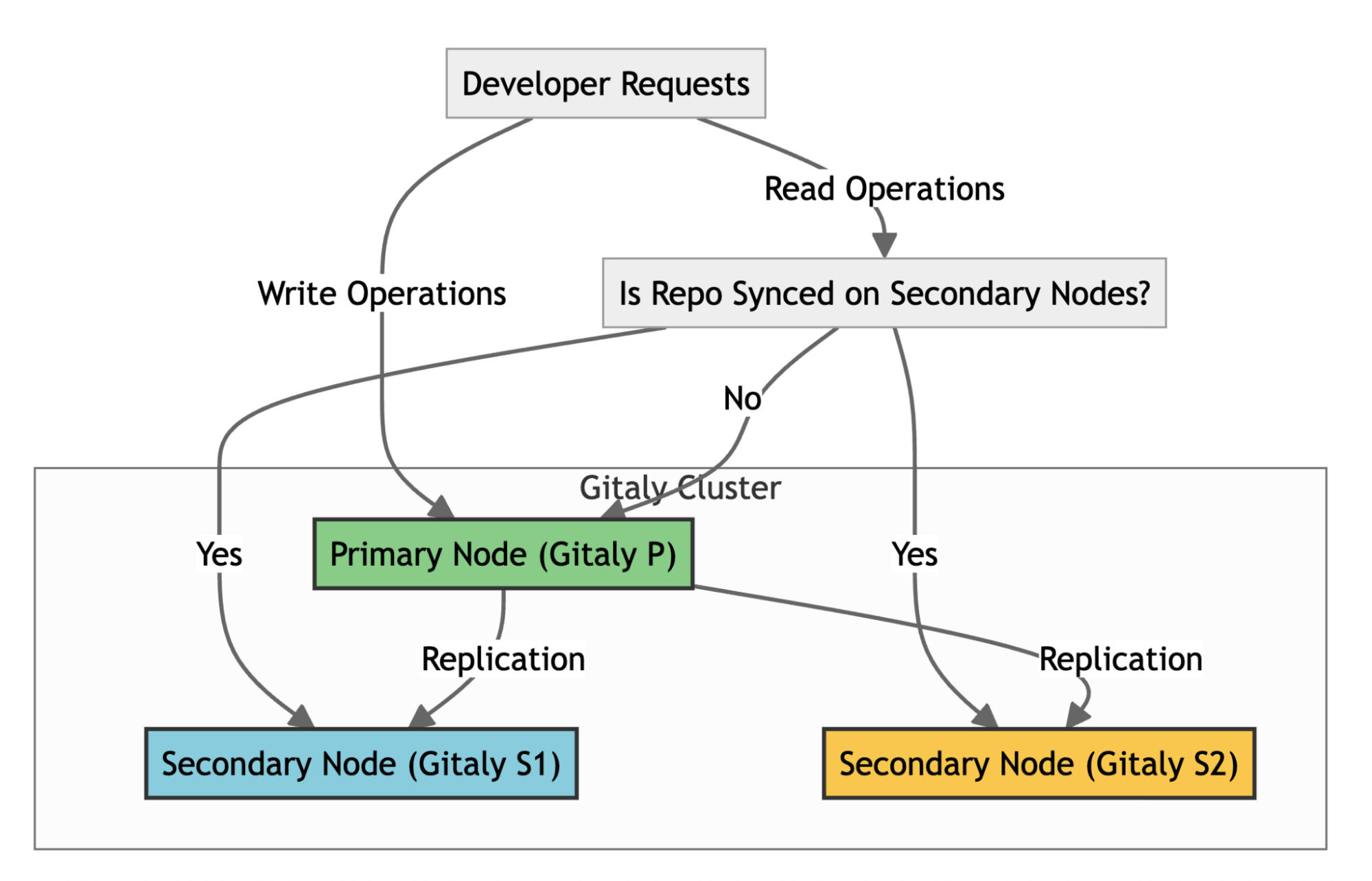
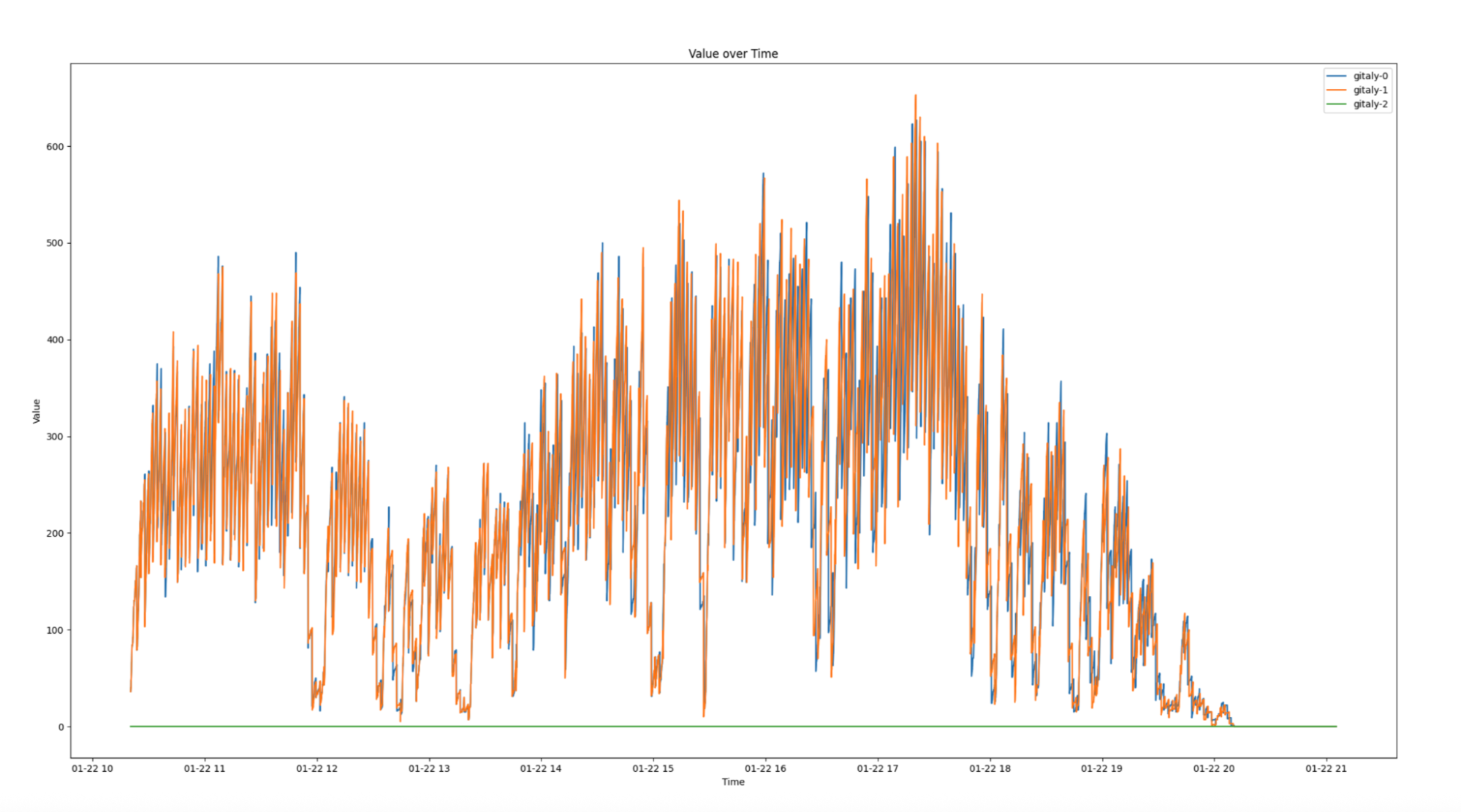
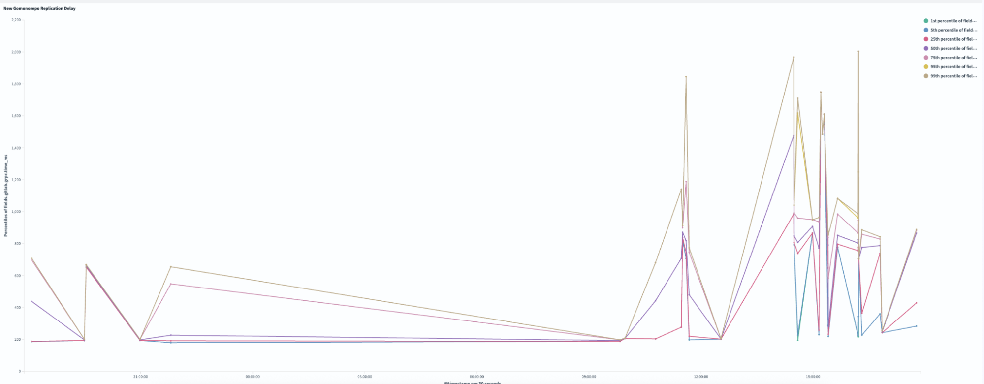
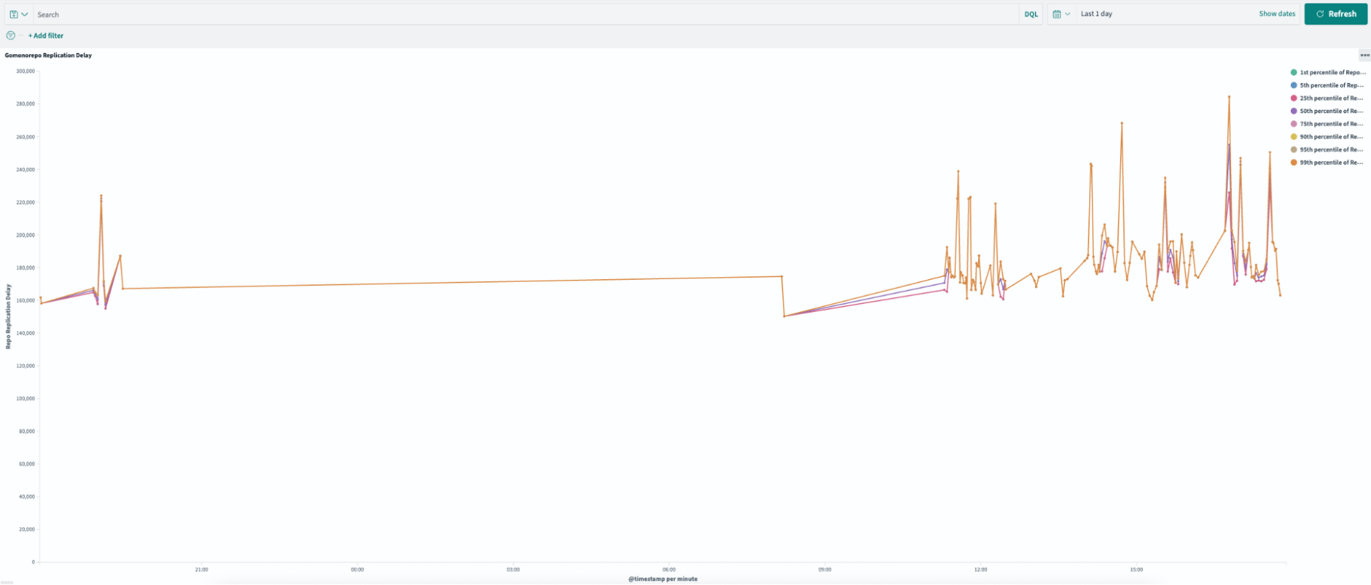
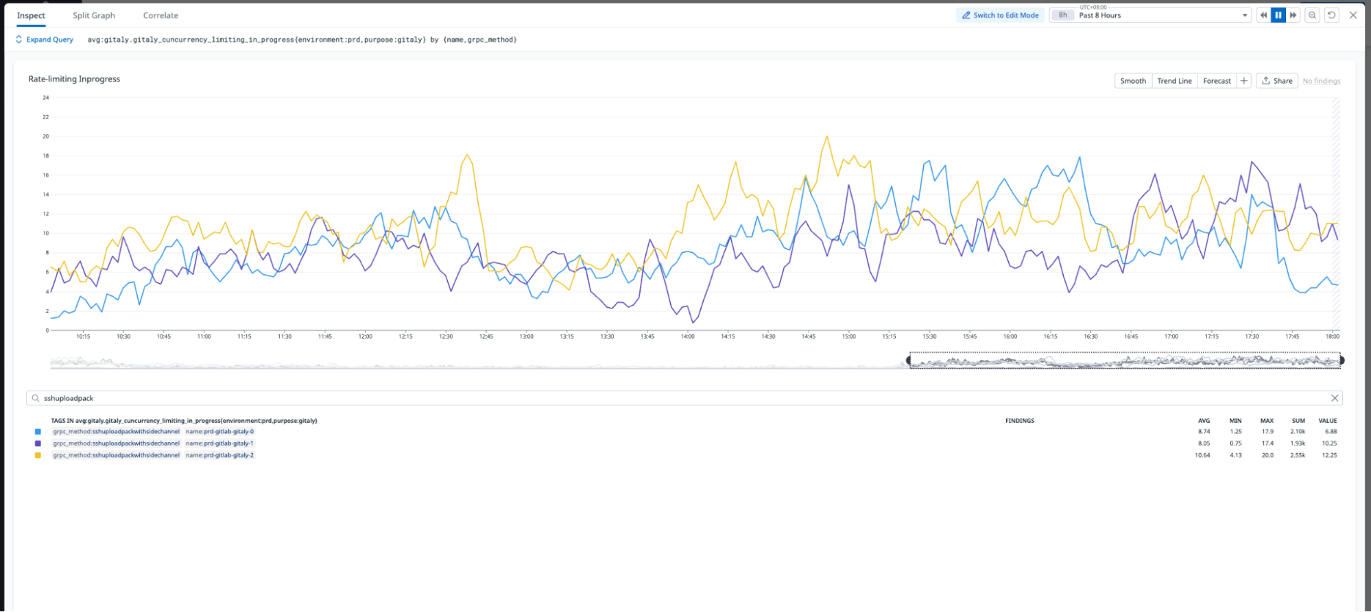
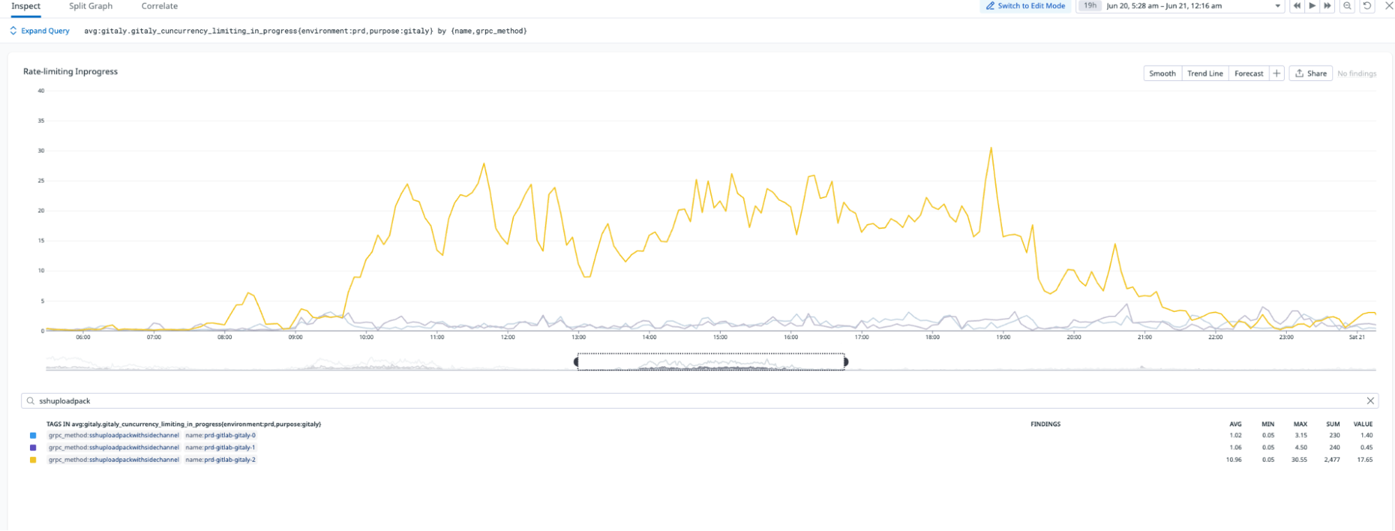


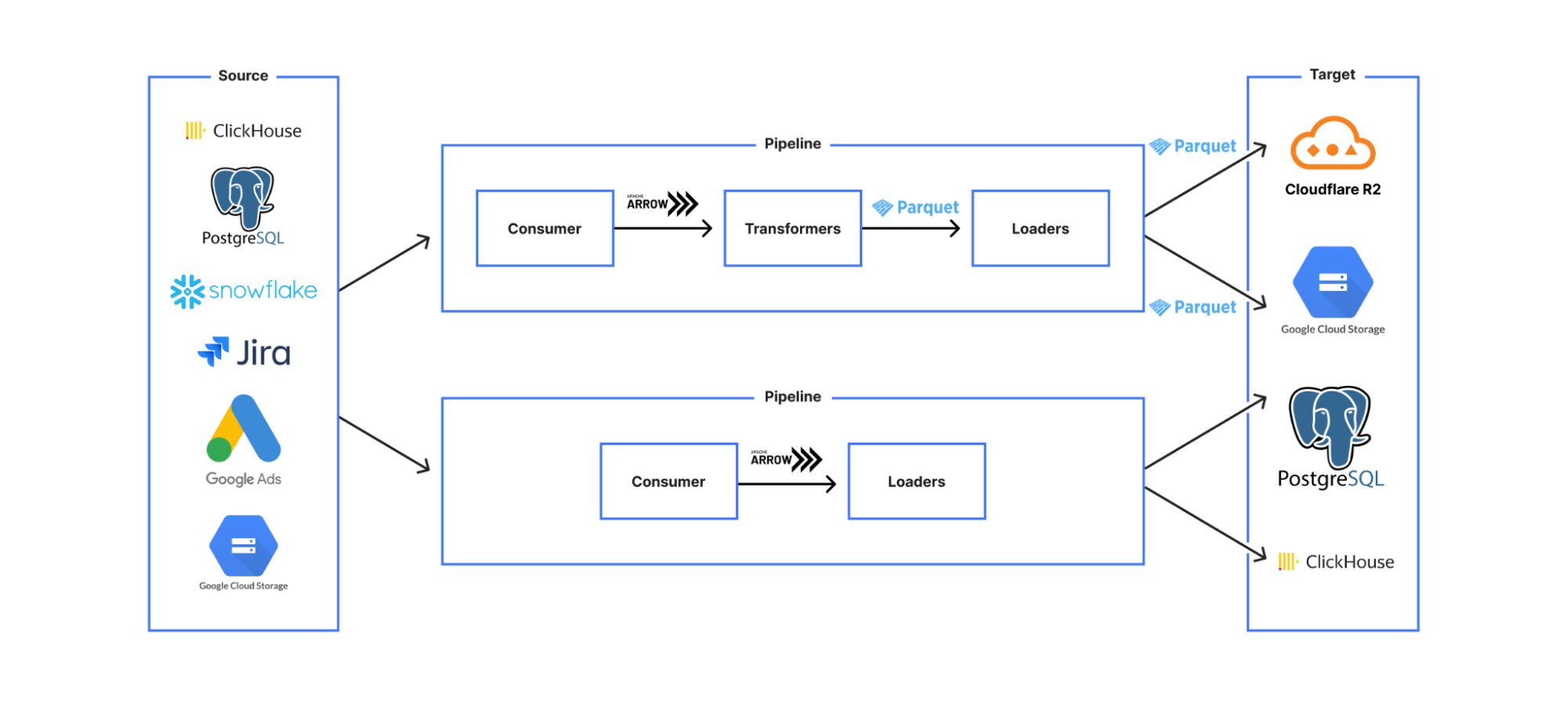
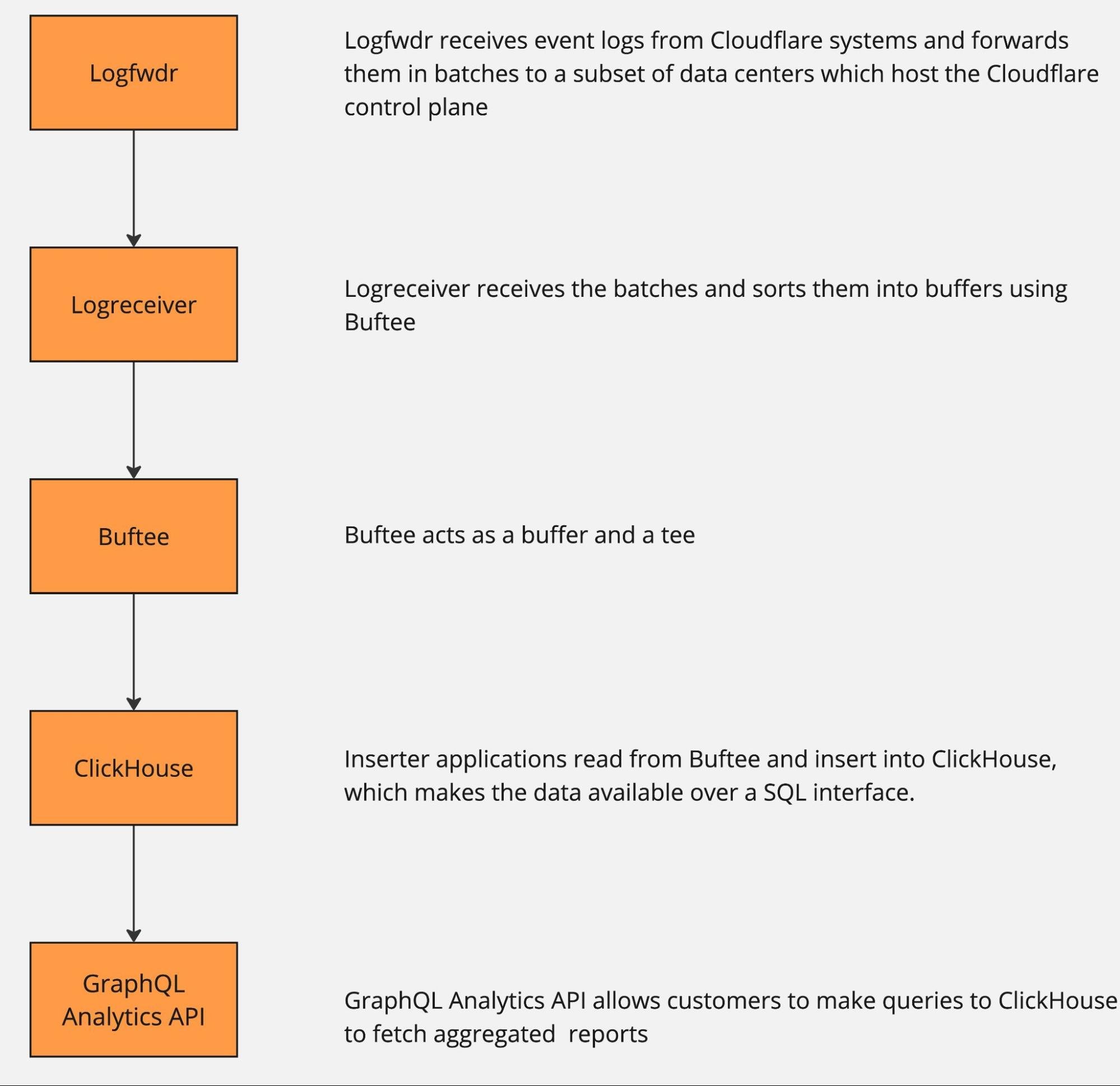

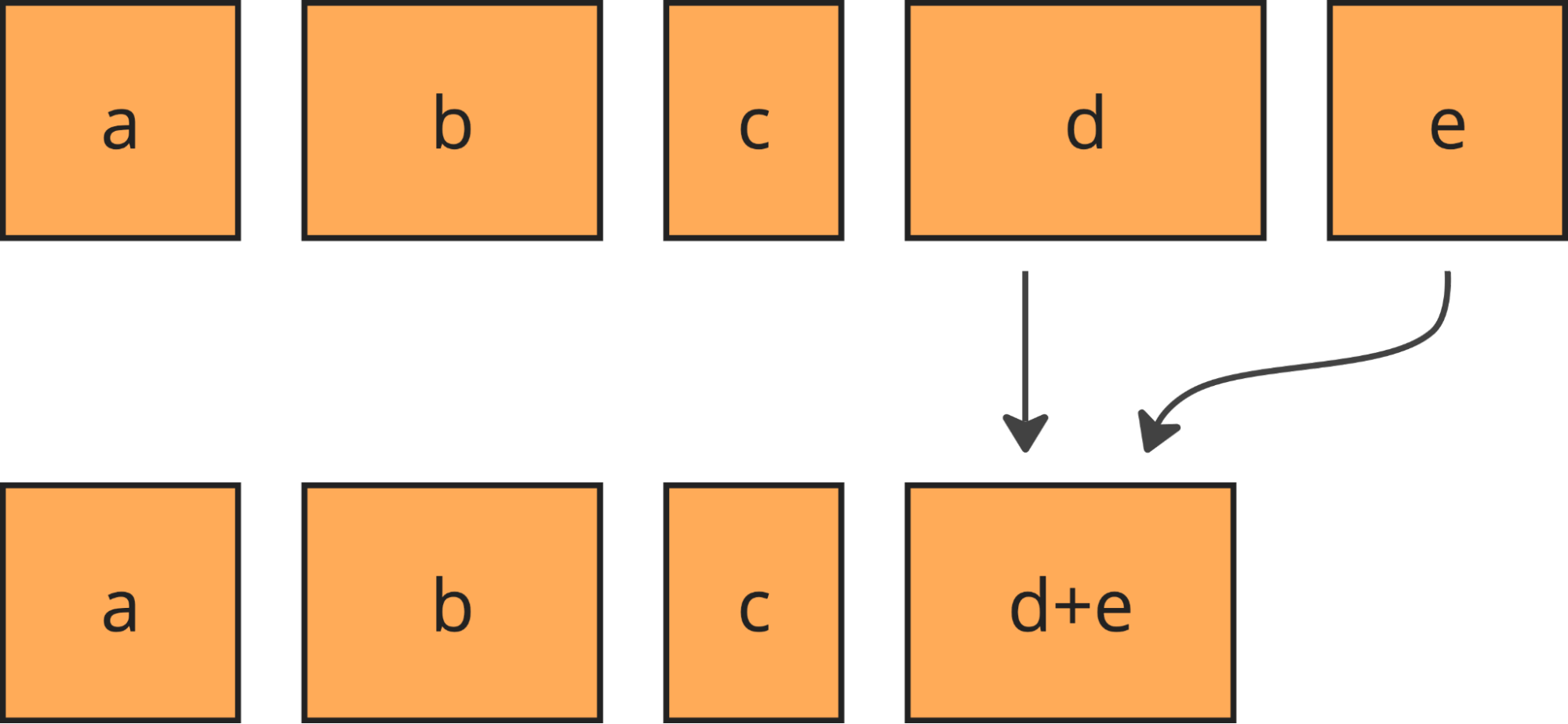
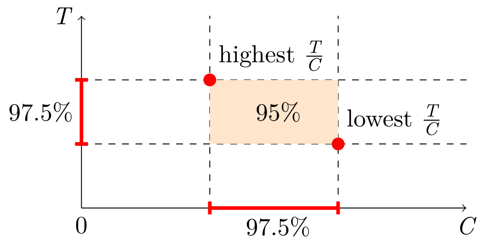
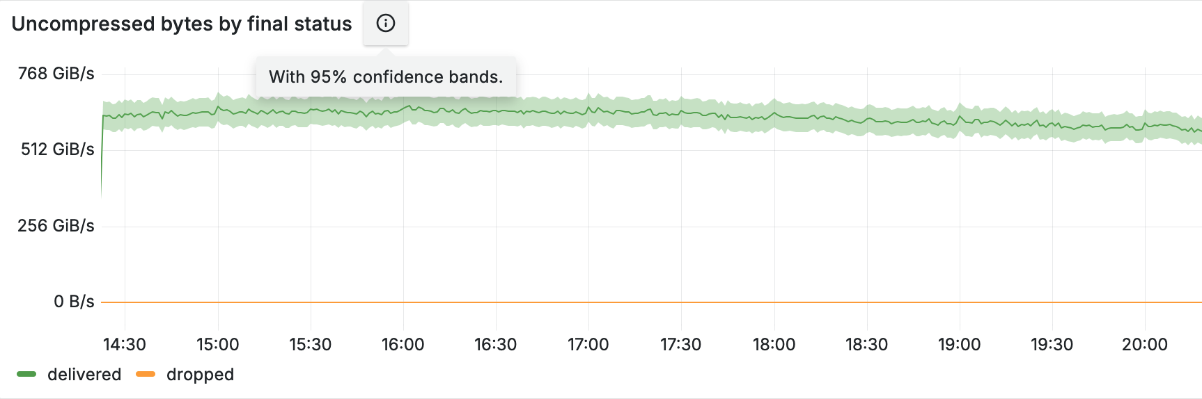
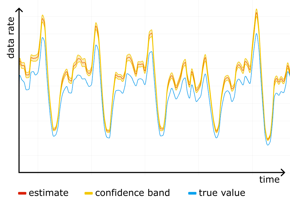

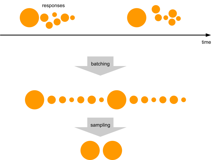
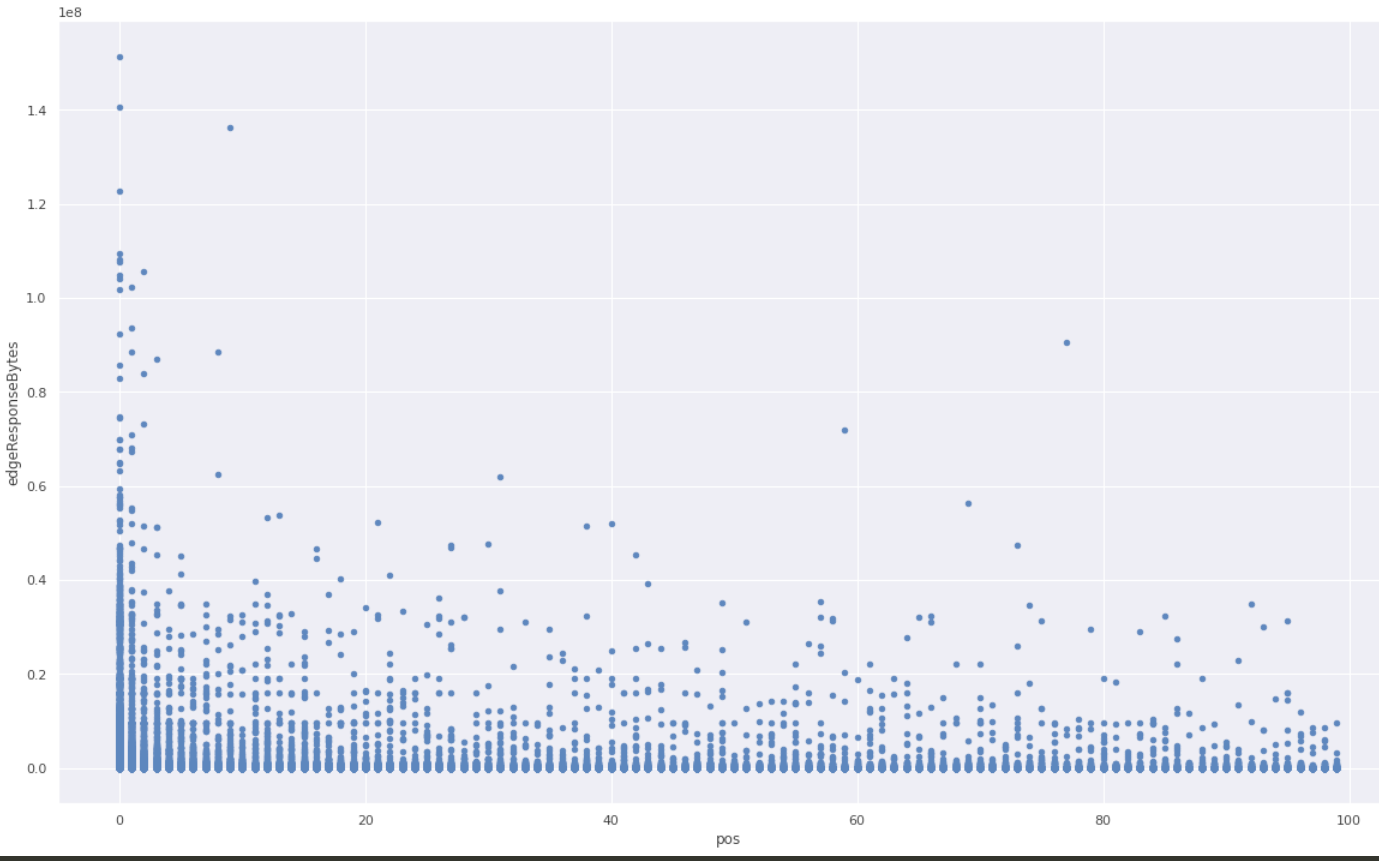
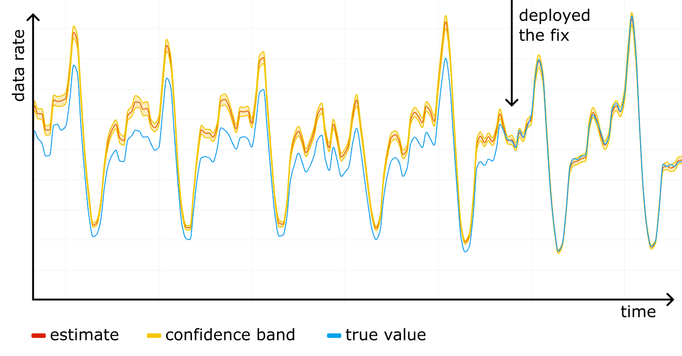

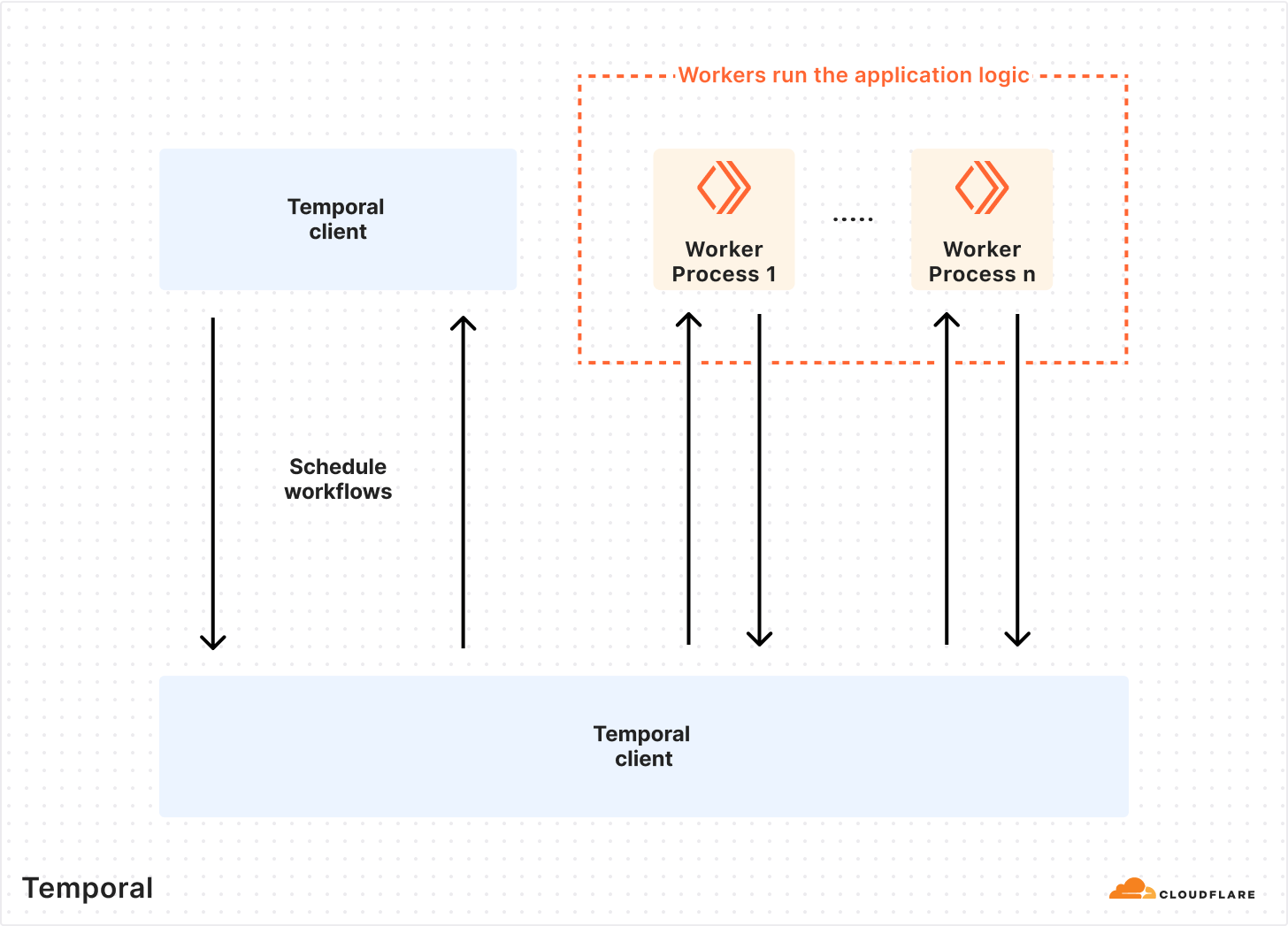
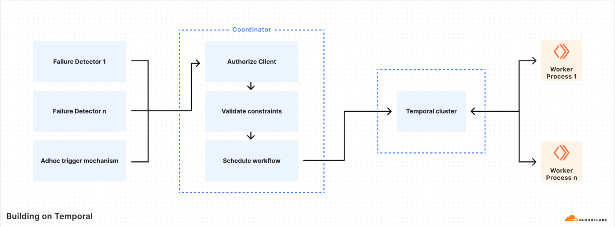
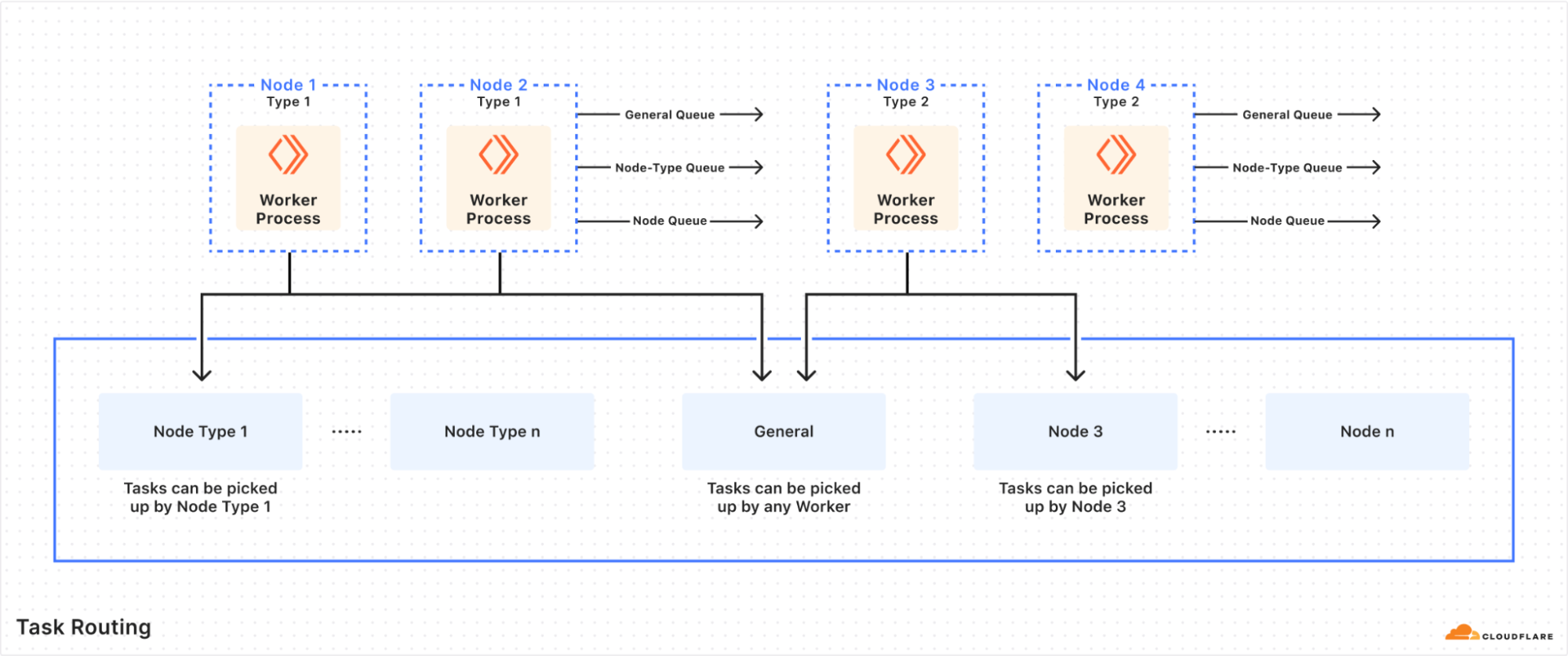
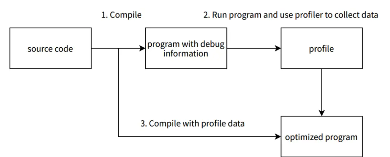
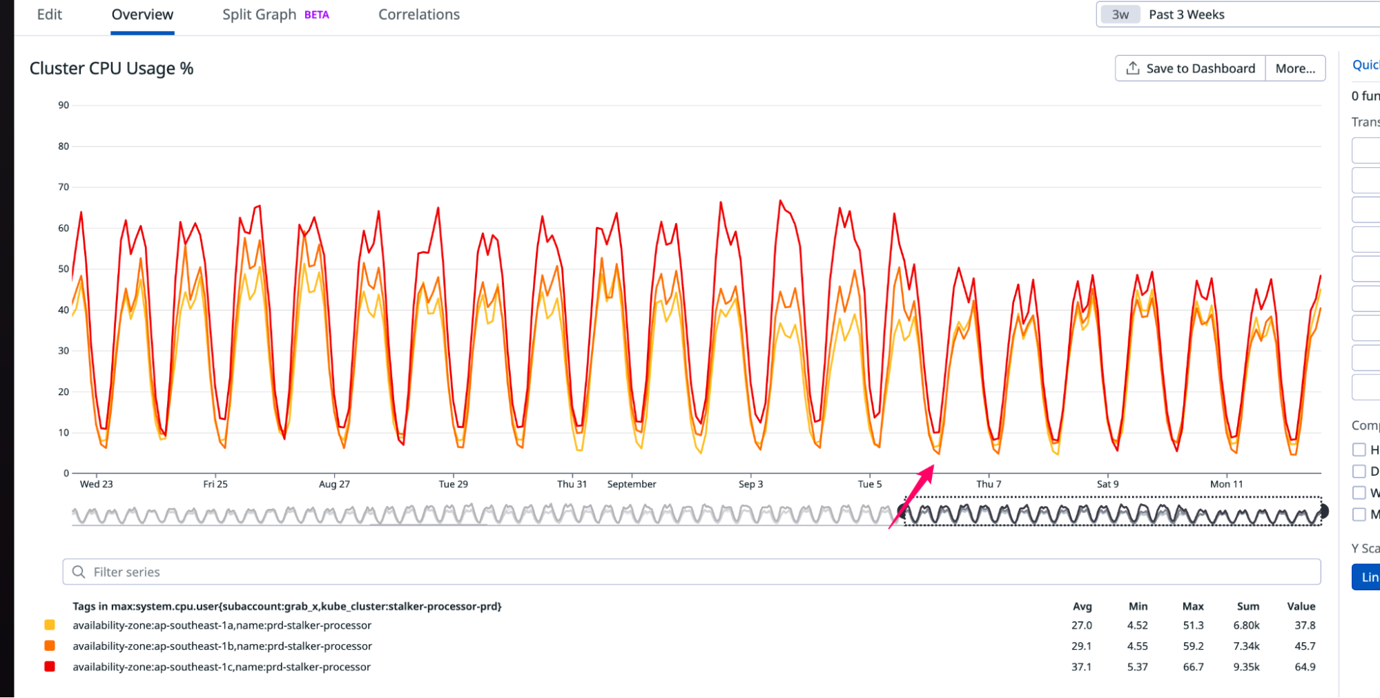
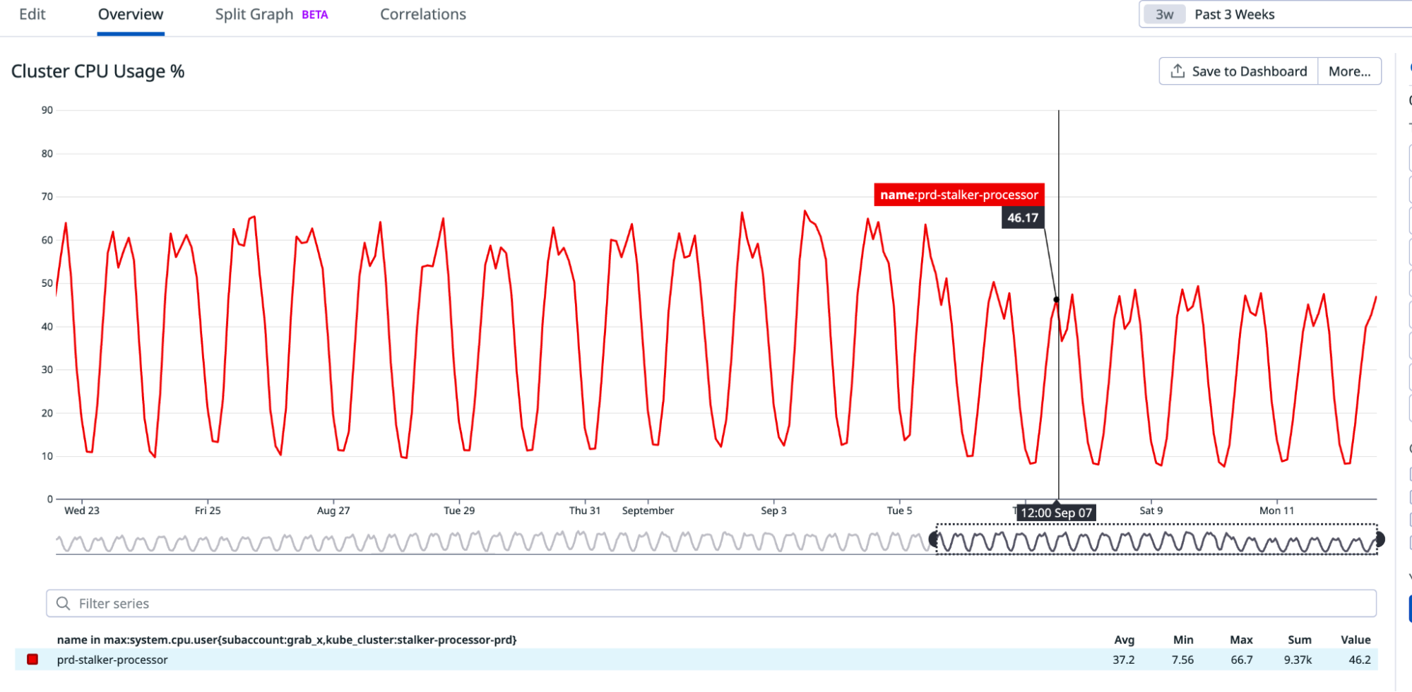
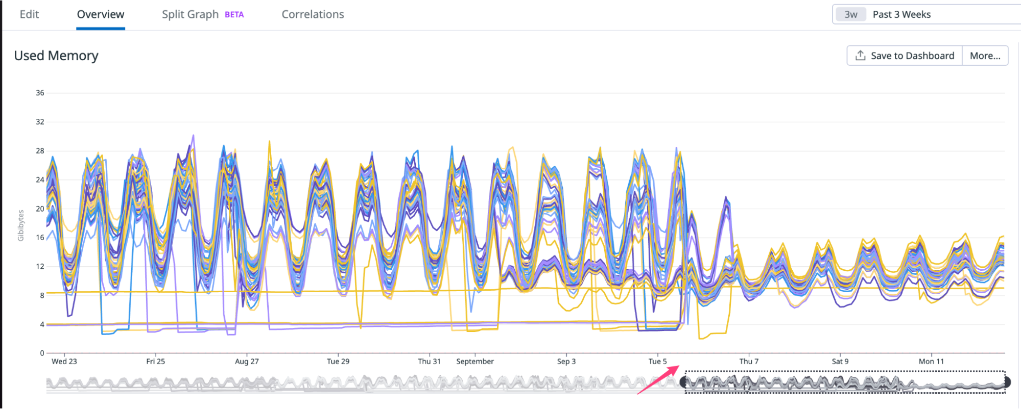
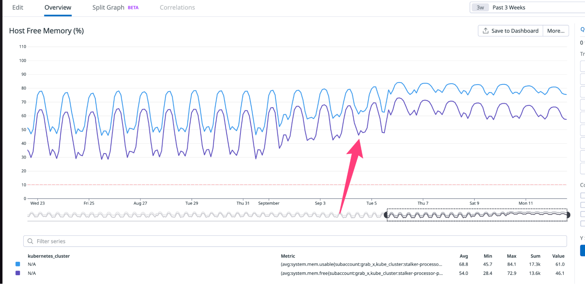
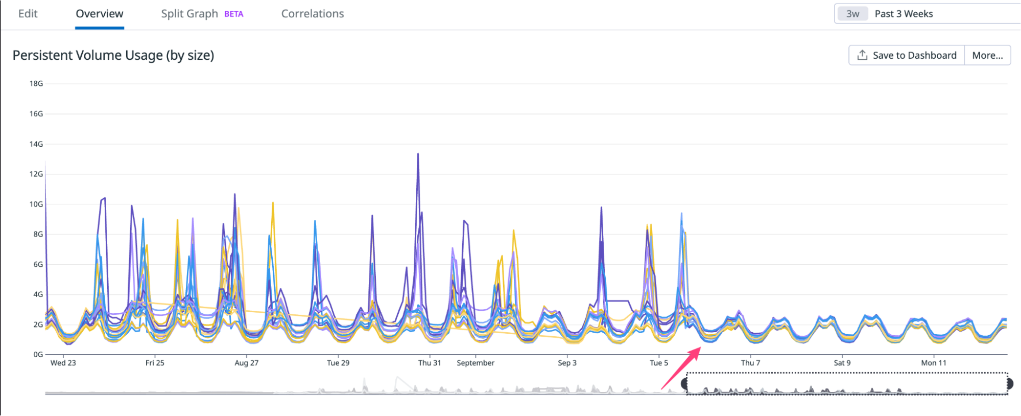
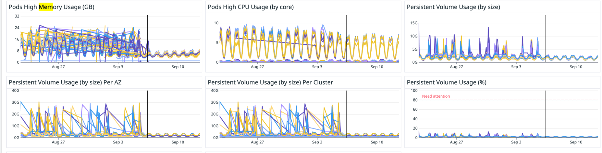
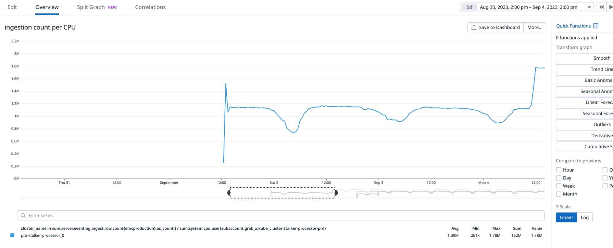
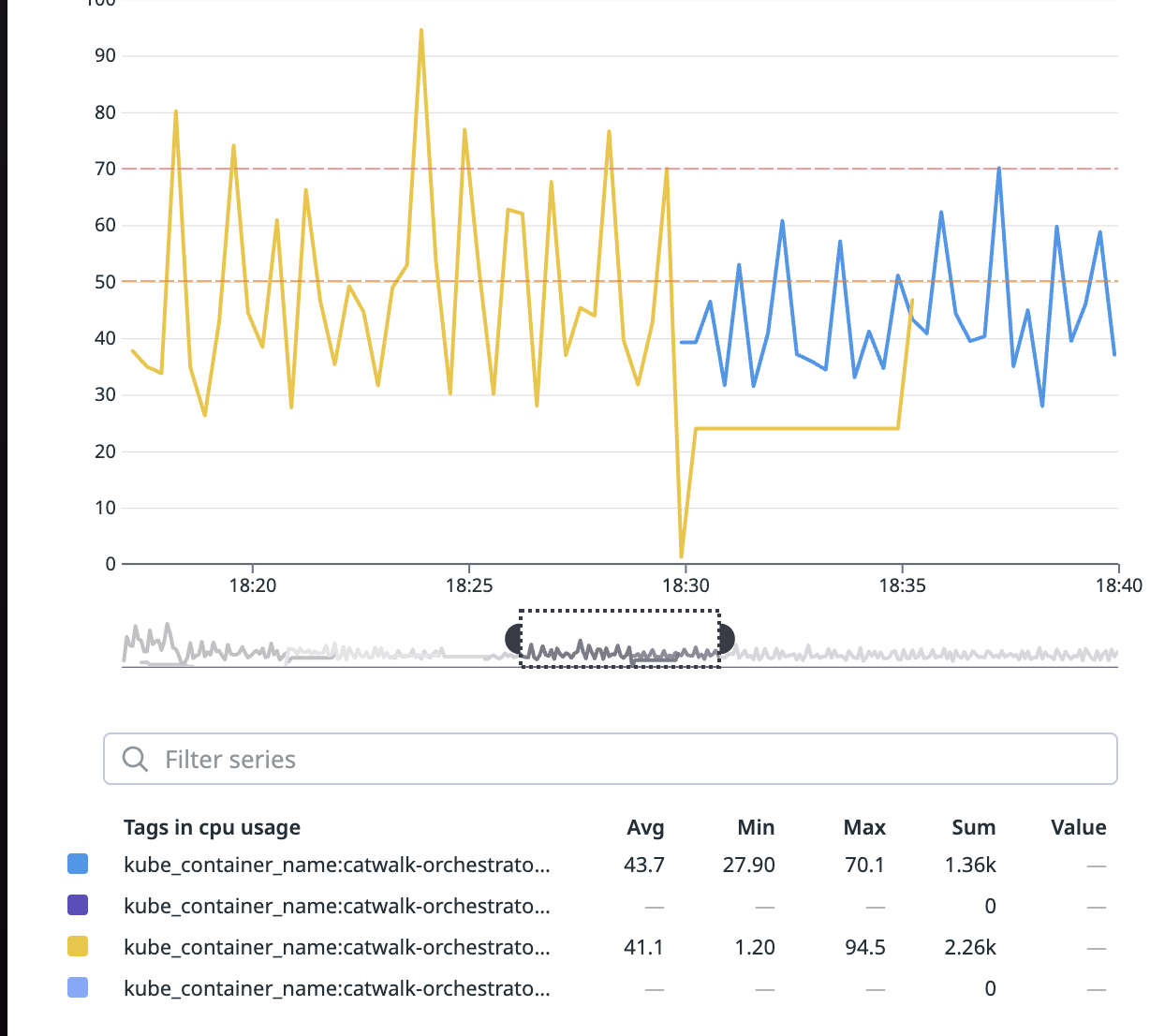
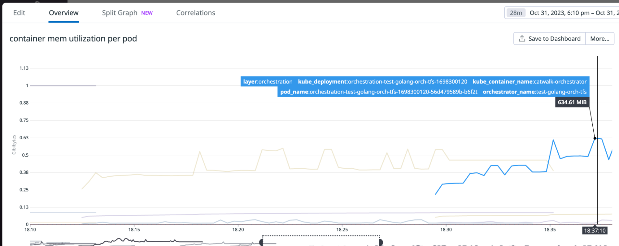


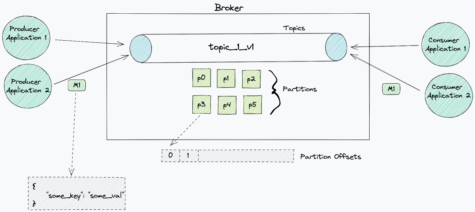
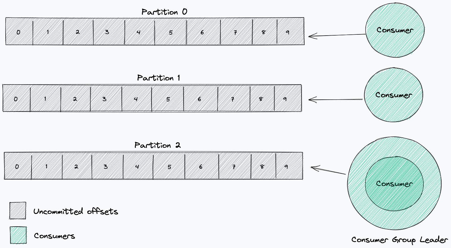
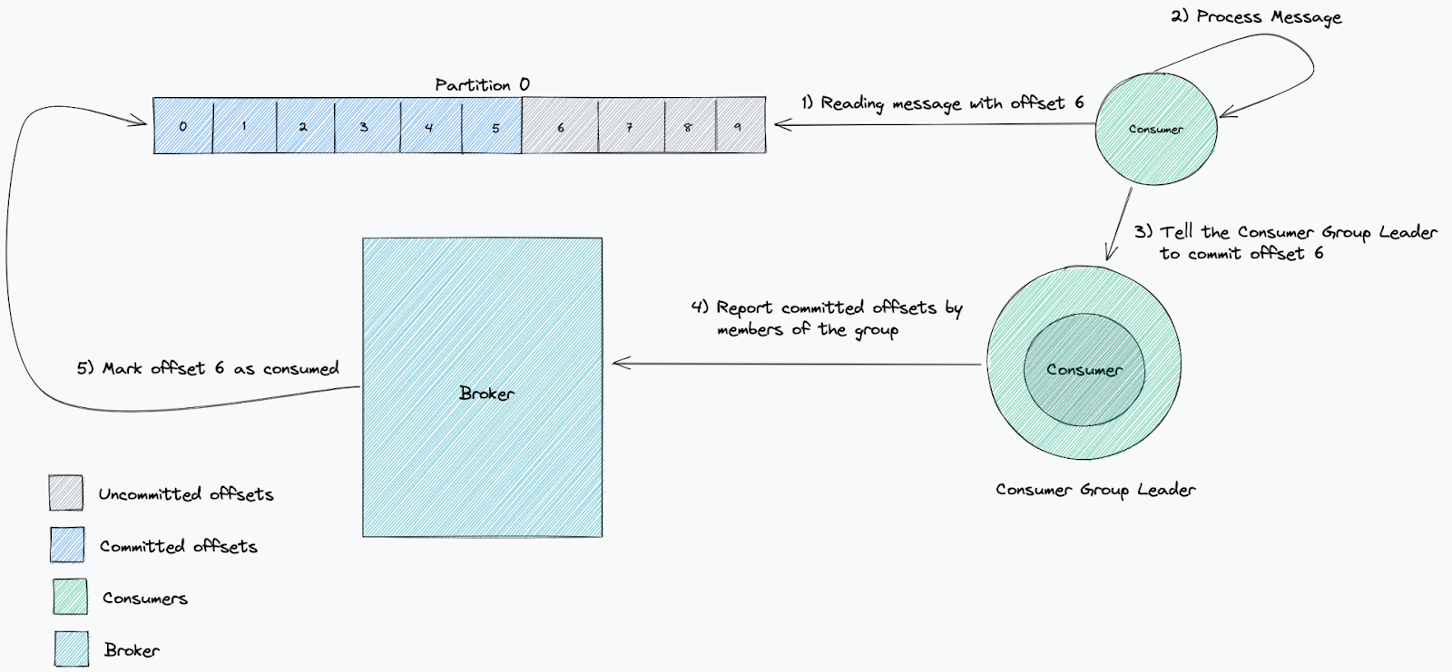
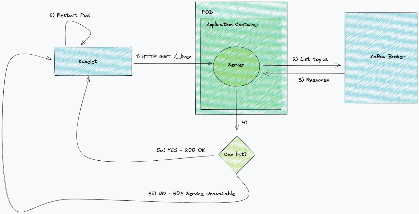
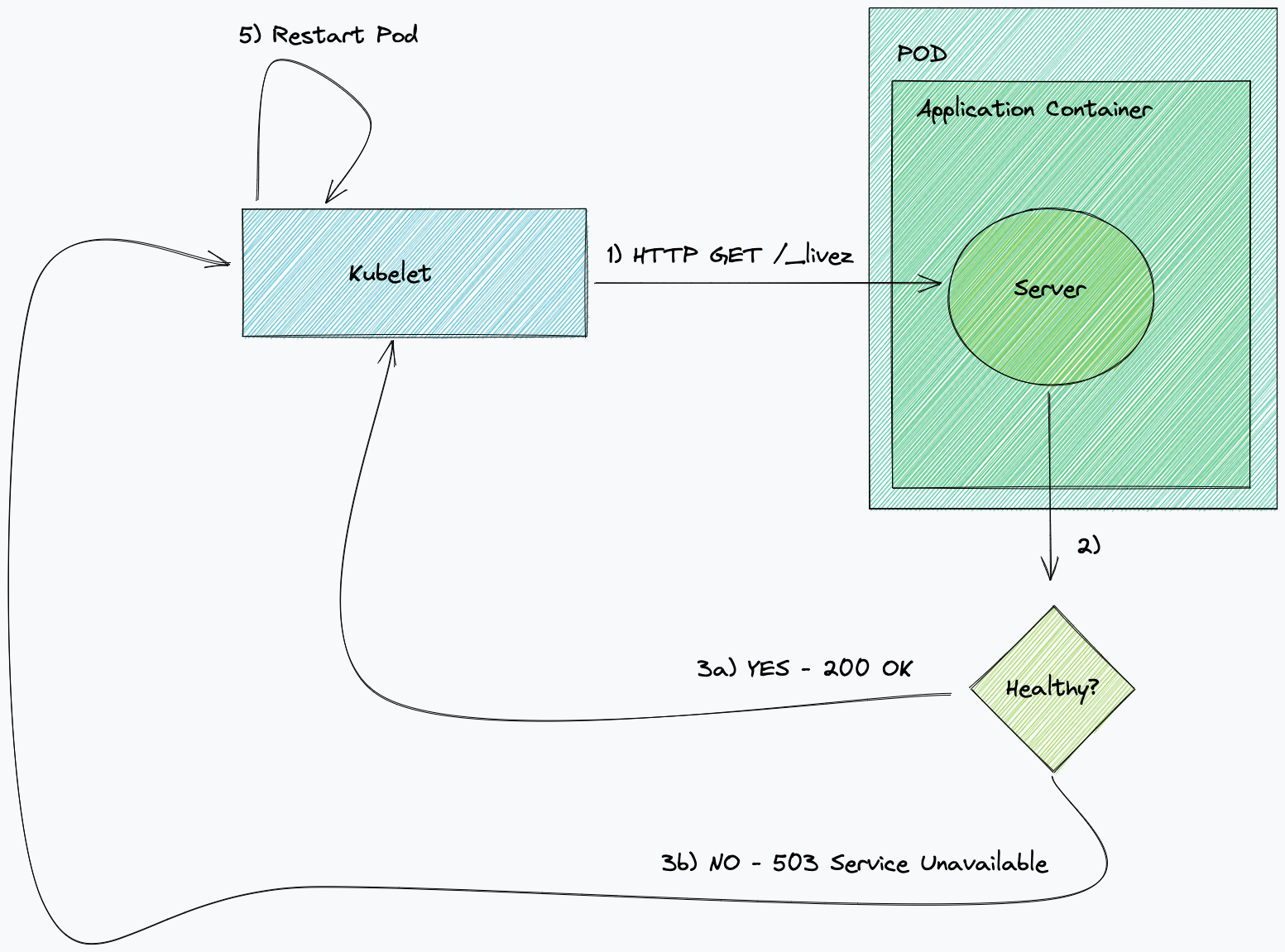
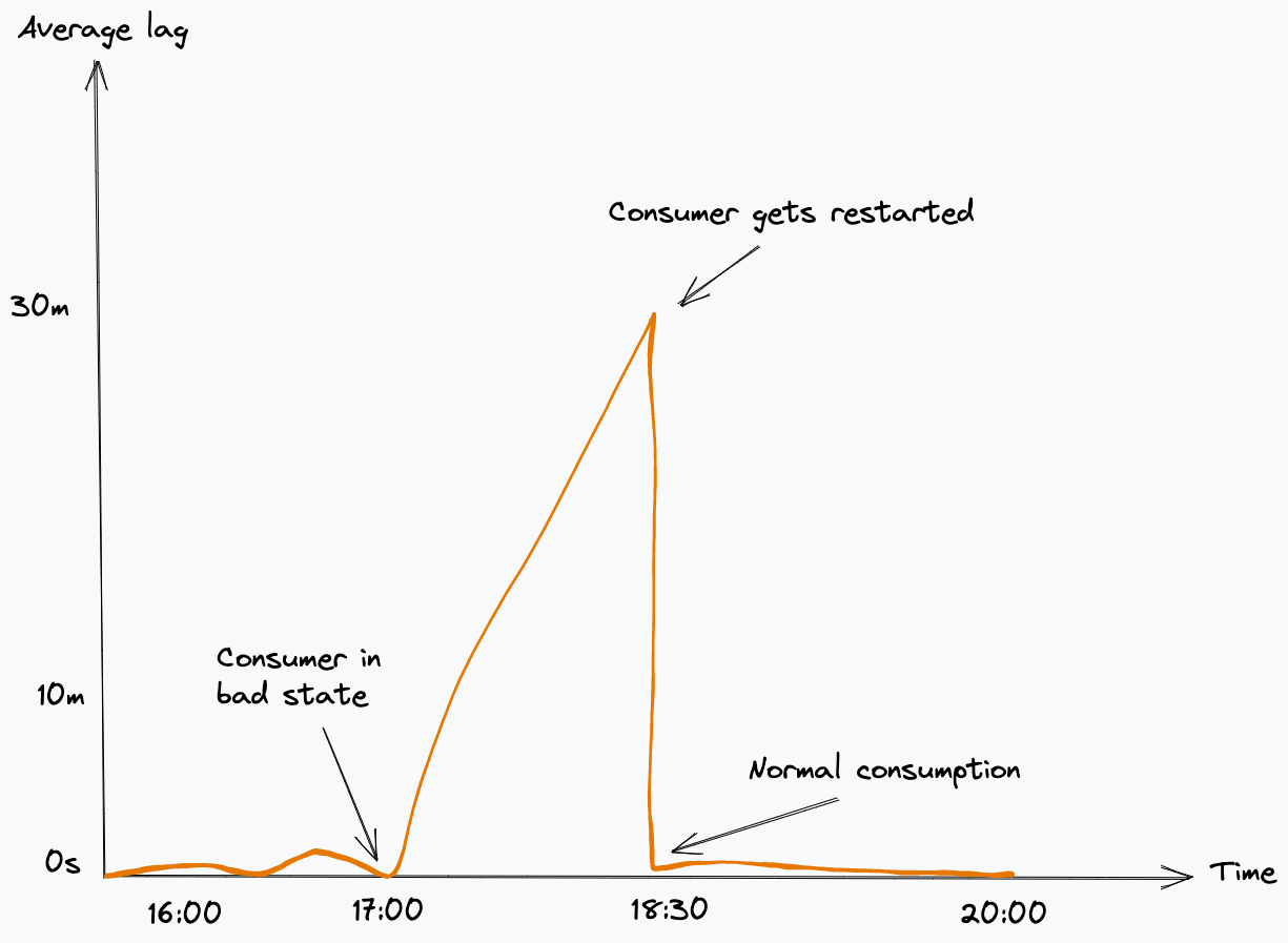
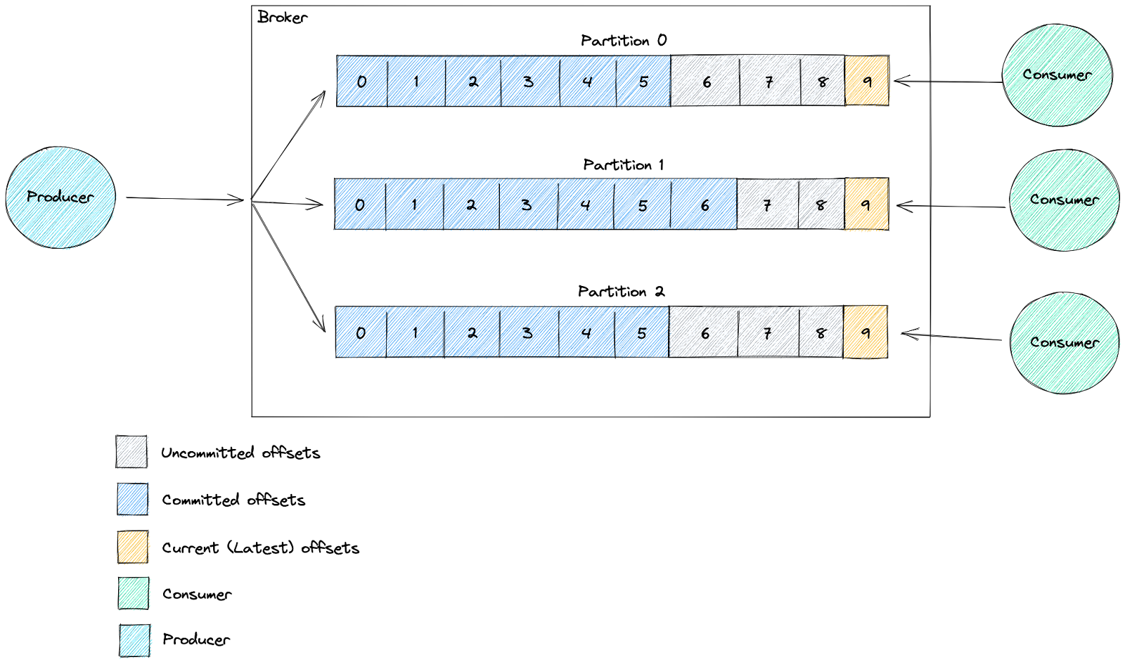
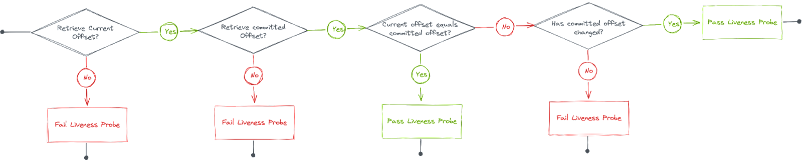


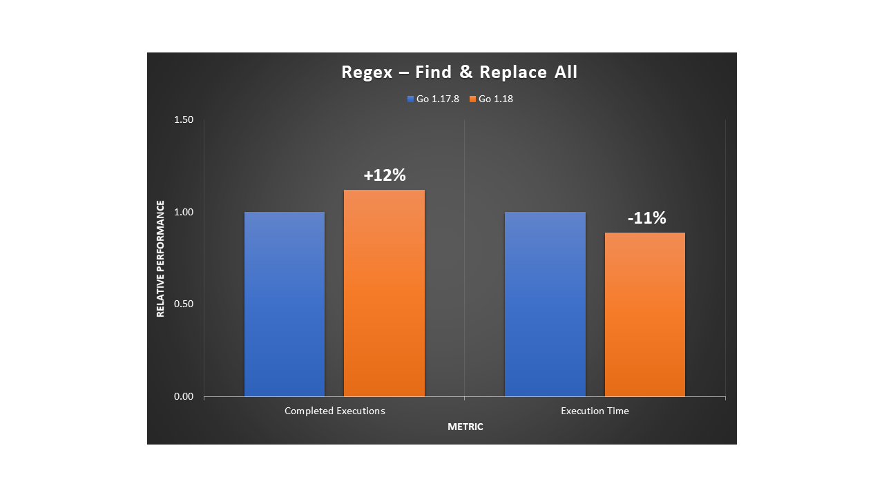


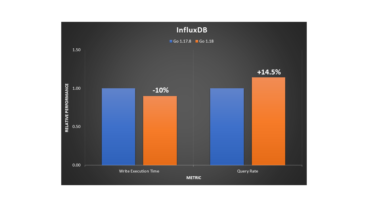
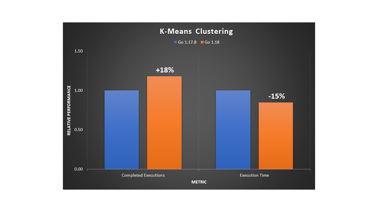

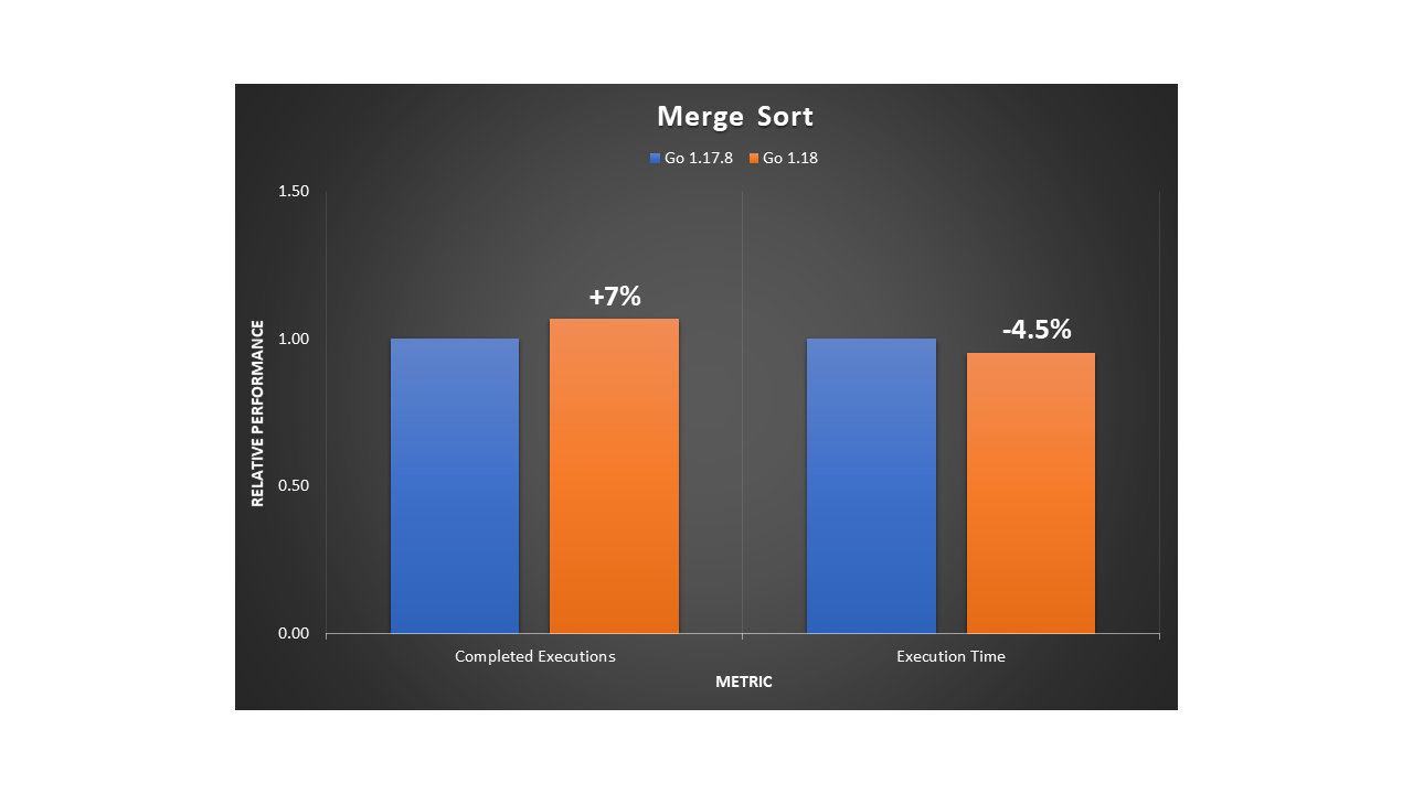
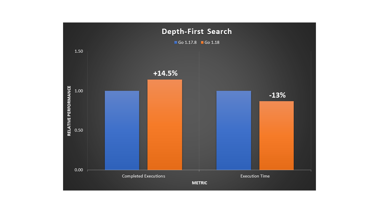


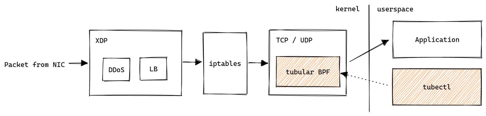

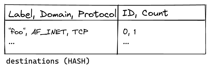
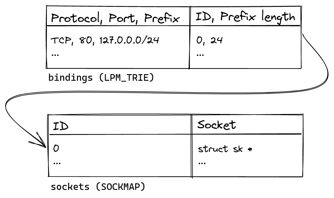


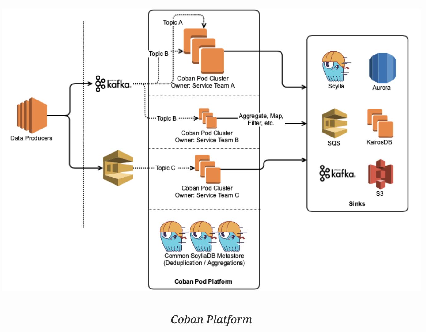
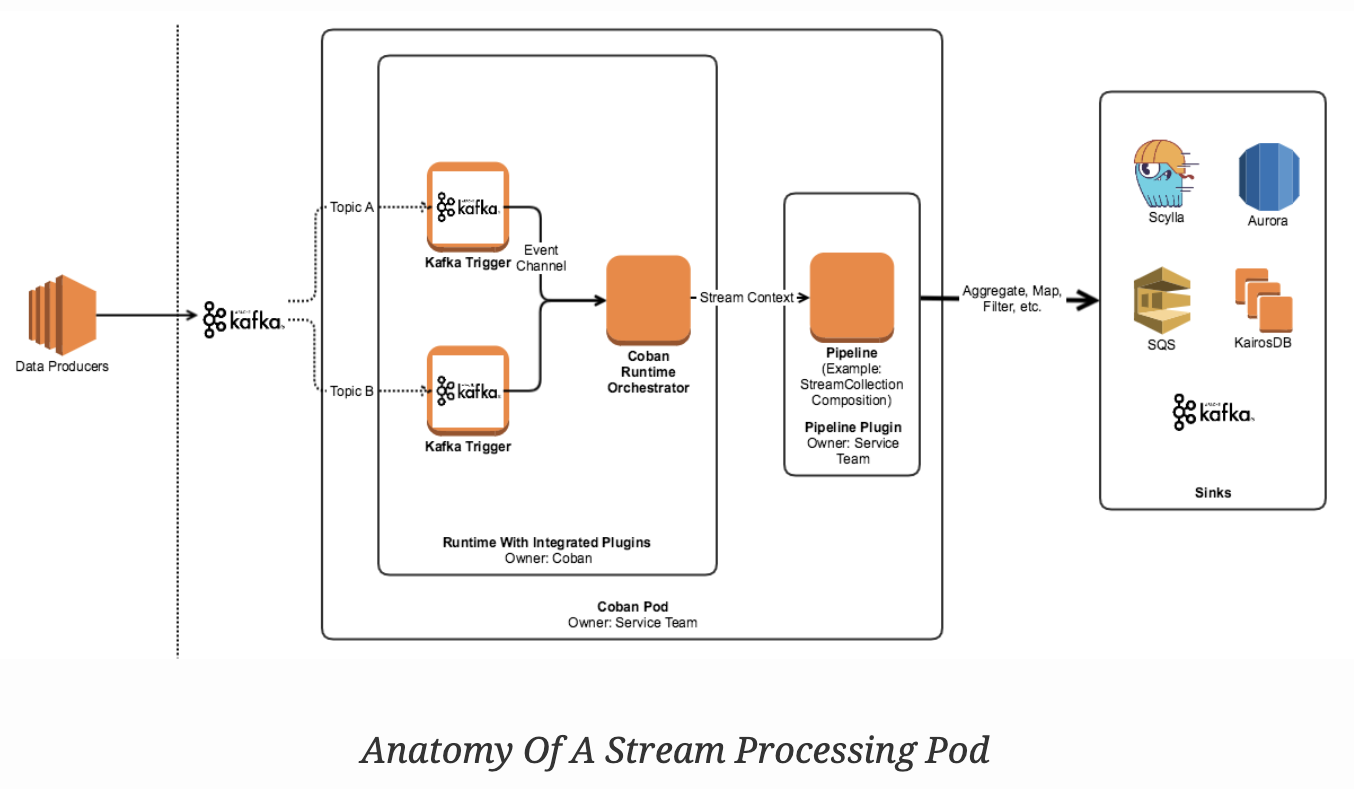
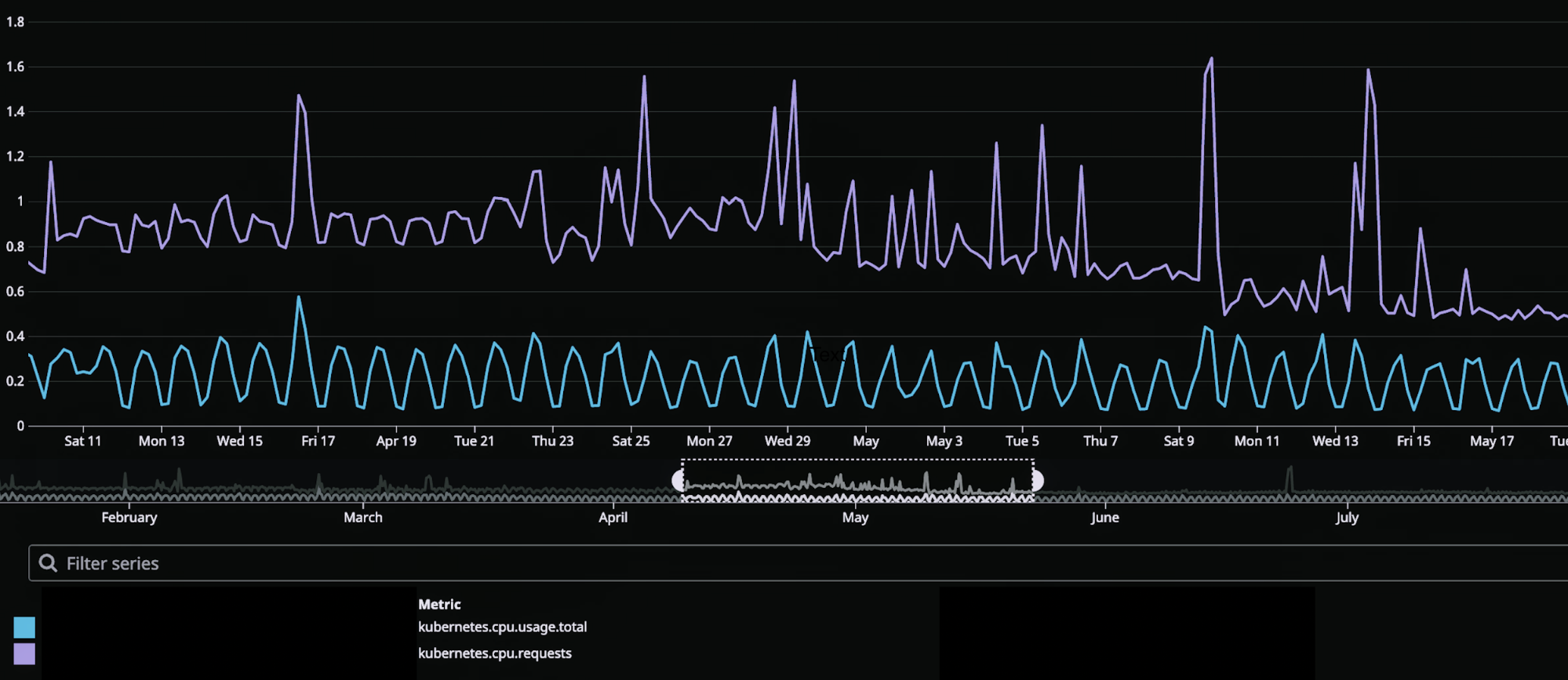