This is the first entry of a multi-part blog series describing how we built a Real-Time Distributed Graph (RDG). In Part 1, we will discuss the motivation for creating the RDG and the architecture of the data processing pipeline that populates it.
Introduction
The Netflix product experience historically consisted of a single core offering: streaming video on demand. Our members logged into the app, browsed, and watched titles such as Stranger Things, Squid Game, and Bridgerton. Although this is still the core of our product, our business has changed significantly over the last few years. For example, we introduced ad-supported plans, live programming events (e.g., Jake Paul vs. Mike Tyson and NFL Christmas Day Games), and mobile games as part of a Netflix subscription. This evolution of our business has created a new class of problems where we have to analyze member interactions with the app across different business verticals. Let’s walk through a simple example scenario:
Imagine a Netflix member logging into the app on their smartphone and beginning to watch an episode of Stranger Things.
Eventually, they decide to watch on a bigger screen, so they log into the app on a smart TV in their home and continue watching the same episode.
Finally, after completing the episode, they log into the app on their tablet and play the game “Stranger Things: 1984”.
We want to know that these three activities belong to the same member, despite occurring at different times and across various devices. In a traditional data warehouse, these events would land in at least two different tables and may be processed at different cadences. But in a graph system, they become connected almost instantly. Ultimately, analyzing member interactions in the app across domains empowers Netflix to create more personalized and engaging experiences.
In the early days of our business expansion, discovering these relationships and contextual insights was extremely difficult. Netflix is famous for adopting a microservices architecture — hundreds of microservices developed and maintained by hundreds of individual teams. Some notable benefits of microservices are:
Service Decomposition: The overall platform is separated into smaller services, each responsible for a specific business capability. This modularity allows for independent service development, deployment, and scaling.
Data Isolation: Each service manages its own data, reducing interdependencies. This allows teams to choose the most suitable data schemas and storage technologies for their services.
However, these benefits also led to drawbacks for our data science and engineering partners. In practice, the separation of business concerns and service development ultimately resulted in a separation of data. Manually stitching data together from our data warehouse and siloed databases was an onerous task for our partners. Our data engineering team recognized we needed a solution to process and store our enormous swath of interconnected data while enabling fast querying to discover insights. Although we could have structured the data in various ways, we ultimately settled on a graph representation. We believe a graph offers key advantages, specifically:
Relationship-Centric Queries: Graphs enable fast “hops” across multiple nodes and edges without expensive joins or manual denormalization that would be required in table-based data models.
Flexibility as Relationships Grow: As new connections and entities emerge, graphs can quickly adapt without significant schema changes or re-architecture.
Pattern and Anomaly Detection: Our stakeholders’ use cases often require identifying hidden relationships, cycles, or groupings in the data — capabilities much more naturally expressed and efficiently executed using graph traversals than siloed point lookups.
This is why we set out to build a Real-Time Distributed Graph, or “RDG” for short.
Ingestion and Processing
Three main layers in the system power the RDG:
Ingestion and Processing — receive events from disparate upstream data sources and use them to generate graph nodes and edges.
Storage — write nodes and edges to persistent data stores.
Serving — expose ways for internal clients to query graph nodes and edges.
The rest of this post will focus on the first layer, while subsequent posts in this blog series will cover the other layers. The diagram below depicts a high-level overview of the ingestion and processing pipeline:
Building and updating the RDG in real-time requires continuously processing vast volumes of incoming data. Batch processing systems and traditional data warehouses cannot offer the low latency needed to maintain an up-to-date graph that supports real-time applications. We opted for a stream processing architecture, enabling us to update the graph’s data as events happen, thus minimizing delay and ensuring the system reflects the latest member interactions within the Netflix app.
Kafka as the Ingestion Backbone
Member actions in the Netflix app are published to our API Gateway, which then writes them as records to Apache Kafka topics. Kafka is the mechanism through which internal data applications can consume these events. It provides durable, replayable streams that downstream processors, such as Apache Flink jobs, can consume in real-time.
Our team’s applications consume several different Kafka topics, each generating up to roughly 1 million messages per second. Topic records are encoded in the Apache Avro format, and Avro schemas are persisted in an internal centralized schema registry. In order to strike a balance between maintaining data availability and managing the financial expenses of storage infrastructure, we tailor retention policies for each topic according to its throughput and record size. We also persist topic records to Apache Iceberg data warehouse tables, which allows us to backfill data in scenarios where older data is no longer available in the Kafka topics.
Processing Data with Apache Flink
The event records in the Kafka streams are ingested by Flink jobs. We chose Flink because of its strong capabilities around near-real-time event processing. There is also robust internal platform support for Flink within Netflix, which allows jobs to integrate with Kafka and various storage backends seamlessly. At a high level, the anatomy of an RDG Flink job looks like this:
For the sake of simplicity, the diagram above depicts a basic flow in which a member logs into their Netflix account and begins watching an episode of Stranger Things. Reading the diagram from left to right:
The actions of logging into the app and watching the Stranger Things episode are ultimately written as events to Kafka topics.
The Flink job consumes event records from the upstream Kafka topics.
Next, we have a series of Flink processor functions that:
Apply filtering and projections to remove noise based on the individual fields that are present — or in some cases, not present — in the events.
Enrich events with additional metadata, which are stored and accessed by the processor functions via side inputs.
Transform events into graph primitives — nodes representing entities (e.g., member accounts and show/movie titles), and edges representing relationships or interactions between them. In this example, the diagram only shows a few nodes and an edge to keep things simple. However, in reality, we create and update up to a few dozen different nodes and edges, depending on the member actions that occurred within the Netflix app.
Buffer, detect, and deduplicate overlapping updates that occur to the same nodes and edges within a small, configurable time window. This step reduces the data throughput we publish downstream. It is implemented using stateful process functions and timers.
Publish nodes and edges records to Data Mesh, an abstraction layer that connects data applications and storage systems. We write a total (nodes + edges) of more than 5 million records per second to Data Mesh, which handles persisting the records to various data stores that other internal services can query.
From One Job to Many: Scaling Flink the Hard Way
Initially, we tried having just one Flink job that consumed all the Kafka source topics. However, this quickly became a big operational headache since different topics can have different data volumes and throughputs at different times during the day. Consequently, tuning the monolithic Flink job became extremely difficult — we struggled to find CPU, memory, job parallelism, and checkpointing interval configurations that ensured job stability.
Instead, we pivoted to having a 1:1 mapping from the Kafka source topic to the consuming Flink job. Although this led to additional operational overhead due to more jobs to develop and deploy, each job has been much simpler to maintain, analyze, and tune.
Similarly, each node and edge type is written to a separate Kafka topic. This means we have significantly more Kafka topics to manage. However, we decided the tradeoff of having bespoke tuning and scaling per topic was worth it. We also designed the graph data model to be as generic and flexible as possible, so adding new types of nodes and edges would be an infrequent operation.
Acknowledgements
We would be remiss if we didn’t give a special shout-out to our stunning colleagues who work on the internal Netflix data platform. Building the RDG was a multi-year effort that required us to design novel solutions, and the investments and foundations from our platform teams were critical to its successful creation. You make the lives of Netflix data engineers much easier, and the RDG would not exist without your diligent collaboration!
—
Thanks for reading the first season of the RDG blog series; stay tuned for Season 2, where we will go over the storage layer containing the graph’s various nodes and edges.
Netflix operates at a massive scale, serving hundreds of millions of users with diverse content and features. Behind the scenes, ensuring data consistency, reliability, and efficient operations across various services presents a continuous challenge. At the heart of many critical functions lies the concept of a Write-Ahead Log (WAL) abstraction. At Netflix scale, every challenge gets amplified. Some of the key challenges we encountered include:
Accidental data loss and data corruption in databases
System entropy across different datastores (e.g., writing to Cassandra and Elasticsearch)
Handling updates to multiple partitions (e.g., building secondary indices on top of a NoSQL database)
Data replication (in-region and across regions)
Reliable retry mechanisms forreal time data pipeline at scale
Bulk deletes to database causing OOM on the Key-Value nodes
All the above challenges either resulted in production incidents or outages, consumed significant engineering resources, or led to bespoke solutions and technical debt. During one particular incident, a developer issued an ALTER TABLE command that led to data corruption. Fortunately, the data was fronted by a cache, so the ability to extend cache TTL quickly together with the app writing the mutations to Kafka allowed us to recover. Absent the resilience features on the application, there would have been permanent data loss. As the data platform team, we needed to provide resilience and guarantees to protect not just this application, but all the critical applications we have at Netflix.
Regarding the retry mechanisms for real time data pipelines, Netflix operates at a massive scale where failures (network errors, downstream service outages, etc.) are inevitable. We needed a reliable and scalable way to retry failed messages, without sacrificing throughput.
With these problems in mind, we decided to build a system that would solve all the aforementioned issues and continue to serve the future needs of Netflix in the online data platform space. Our Write-Ahead Log (WAL) is a distributed system that captures data changes, provides strong durability guarantees, and reliably delivers these changes to downstream consumers. This blog post dives into how Netflix is building a generic WAL solution to address common data challenges, enhance developer efficiency, and power high-leverage capabilities like secondary indices, enable cross-region replication for non-replicated storage engines, and support widely used patterns like delayed queues.
API
Our API is intentionally simple, exposing just the essential parameters. WAL has one main API endpoint, WriteToLog, abstracting away the internal implementation and ensuring that users can onboard easily.
/** * WAL request message * namespace: Identifier for a particular WAL * lifecycle: How much delay to set and original write time * payload: Payload of the message * target: Details of where to send the payload */ message WriteToLogRequest { string namespace = 1; Lifecycle lifecycle = 2; bytes payload = 3; Target target = 4; }
A namespace defines where and how data is stored, providing logical separation while abstracting the underlying storage systems. Each namespace can be configured to use different queues: Kafka, SQS, or combinations of multiple. Namespace also serves as a central configuration of settings, such as backoff multiplier or maximum number of retry attempts, and more. This flexibility allows our Data Platform to route different use cases to the most suitable storage system based on performance, durability, and consistency needs.
WAL can assume different personas depending on the namespace configuration.
Persona #1 (Delayed Queues)
In the example configuration below, the Product Data Systems (PDS) namespace uses SQS as the underlying message queue, enabling delayed messages. PDS uses Kafka extensively, and failures (network errors, downstream service outages, etc.) are inevitable. We needed a reliable and scalable way to retry failed messages, without sacrificing throughput. That’s when PDS started leveraging WAL for delayed messages.
Below is the namespace configuration for cross-region replication of EVCache using WAL, which replicates messages from a source region to multiple destinations. It uses Kafka under the hood.
Below is the namespace configuration for supporting mutateItems API in Key-Value, where multiple write requests can go to different partitions and have to be eventually consistent. A key detail in the below configuration is the presence of Kafka and durable_storage. These data stores are required to facilitate two phase commit semantics, which we will discuss in detail below.
An important note is that requests to WAL support at-least once semantics due to the underlying implementation.
Under the Hood
The core architecture consists of several key components working together.
Message Producer and Message Consumer separation: The message producer receives incoming messages from client applications and adds them into the queue, while the message consumer processes messages from the queue and sends them to the targets. Because of this separation, other systems can bring their own pluggable producers or consumers, depending on their use cases. WAL’s control plane allows for a pluggable model, which, depending on the use-case, allows us to switch between different message queues.
SQS and Kafka with a dead letter queue by default: Every WAL namespace has its own message queue and gets a dead letter queue (DLQ) by default, because there can be transient errors and hard errors. Application teams using Key-Value abstraction simply need to toggle a flag to enable WAL and get all this functionality without needing to understand the underlying complexity.
Kafka-backed namespaces: handle standard message processing
SQS-backed namespaces: support delayed queue semantics (we added custom logic to go beyond the standard defaults enforced in terms of delay, size limits, etc)
Complex multi-partition scenarios: use queues and durable storage
Target Flexibility: The messages added to WAL are pushed to the target datastores. Targets can be Cassandra databases, Memcached caches, Kafka queues, or upstream applications. Users can specify the target via namespace configuration and in the API itself.
Architecture of WAL
Deployment Model
WAL is deployed using the Data Gateway infrastructure. This means that WAL deployments automatically come with mTLS, connection management, authentication, runtime and deployment configurations out of the box.
Each data gateway abstraction (including WAL) is deployed as a shard. A shard is a physical concept describing a group of hardware instances. Each use case of WAL is usually deployed as a separate shard. For example, the Ads Events service will send requests to WAL shard A, while the Gaming Catalog service will send requests to WAL shard B, allowing for separation of concerns and avoiding noisy neighbour problems.
Each shard of WAL can have multiple namespaces. A namespace is a logical concept describing a configuration. Each request to WAL has to specify its namespace so that WAL can apply the correct configuration to the request. Each namespace has its own configuration of queues to ensure isolation per use case. If the underlying queue of a WAL namespace becomes the bottleneck of throughput, the operators can choose to add more queues on the fly by modifying the namespace configurations. The concept of shards and namespaces is shared across all Data Gateway Abstractions, including Key-Value, Counter, Timeseries, etc. The namespace configurations are stored in a globally replicated Relational SQL database to ensure availability and consistency.
Deployment model of WAL
Based on certain CPU and network thresholds, the Producer group and the Consumer group of each shard will (separately) automatically scale up the number of instances to ensure the service has low latency, high throughput and high availability. WAL, along with other abstractions, also uses the Netflix adaptive load shedding libraries and Envoy to automatically shed requests beyond a certain limit. WAL can be deployed to multiple regions, so each region will deploy its own group of instances.
Solving different flavors of problems with no change to the core architecture
The WAL addresses multiple data reliability challenges with no changes to the core architecture:
Data Loss Prevention: In case of database downtime, WAL can continue to hold the incoming mutations. When the database becomes available again, replay mutations back to the database. The tradeoff is eventual consistency rather than immediate consistency, and no data loss.
Generic Data Replication: For systems like EVCache (using Memcached) and RocksDB that do not support replication by default, WAL provides systematic replication (both in-region and across-region). The target can be another application, another WAL, or another queue — it’s completely pluggable through configuration.
System Entropy and Multi-Partition Solutions: Whether dealing with writes across two databases (like Cassandra and Elasticsearch) or mutations across multiple partitions in one database, the solution is the same — write to WAL first, then let the WAL consumer handle the mutations. No more asynchronous repairs needed; WAL handles retries and backoff automatically.
Data Corruption Recovery: In case of DB corruptions, restore to the last known good backup, then replay mutations from WAL omitting the offending write/mutation.
There are some major differences between using WAL and directly using Kafka/SQS. WAL is an abstraction on the underlying queues, so the underlying technology can be swapped out depending on use cases with no code changes. WAL emphasizes an easy yet effective API that saves users from complicated setups and configurations. We leverage the control plane to pivot technologies behind WAL when needed without app or client intervention.
WAL usage at Netflix
Delay Queue
The most common use case for WAL is as a Delay Queue. If an application is interested in sending a request at a certain time in the future, it can offload its requests to WAL, which guarantees that their requests will land after the specified delay.
Netflix’s Live Origin processes and delivers Netflix live stream video chunks, storing its video data in a Key-Value abstraction backed by Cassandra and EVCache. When Live Origin decides to delete certain video data after an event is completed, it issues delete requests to the Key-Value abstraction. However, the large amount of delete requests in a short burst interfere with the more important real-time read/write requests, causing performance issues in Cassandra and timeouts for the incoming live traffic. To get around this, Key-Value issues the delete requests to WAL first, with a random delay and jitter set for each delete request. WAL, after the delay, sends the delete requests back to Key-Value. Since the deletes are now a flatter curve of requests over time, Key-Value is then able to send the requests to the datastore with no issues.
Requests being spread out over time through delayed requests
Additionally, WAL is used by many services that utilize Kafka to stream events, including Ads, Gaming, Product Data Systems, etc. Whenever Kafka requests fail for any reason, the client apps will send WAL a request to retry the kafka request with a delay. This abstracts away the backoff and retry layer of Kafka for many teams, increasing developer efficiency.
Backoff and delayed retries for clients producing to KafkaBackoff and delayed retries for clients consuming from Kafka
Cross-Region Replication
WAL is also used for global cross-region replication. The architecture of WAL is generic and allows any datastore/applications to onboard for cross-region replication. Currently, the largest use case is EVCache, and we are working to onboard other storage engines.
EVCache is deployed by clusters of Memcached instances across multiple regions, where each cluster in each region shares the same data. Each region’s client apps will write, read, or delete data from the EVCache cluster of the same region. To ensure global consistency, the EVCache client of one region will replicate write and delete requests to all other regions. To implement this, the EVCache client that originated the request will send the request to a WAL corresponding to the EVCache cluster and region.
Since the EVCache client acts as the message producer group in this case, WAL only needs to deploy the message consumer groups. From there, the multiple message consumers are set up to each target region. They will read from the Kafka topic, and send the replicated write or delete requests to a Writer group in their target region. The Writer group will then go ahead and replicate the request to the EVCache server in the same region.
EVCache Global Cross-Region Replication Implemented through WAL
The biggest benefits of this approach, compared to our legacy architecture, is being able to migrate from multi-tenant architecture to single tenant architecture for the most latency sensitive applications. For example, Live Origin will have its own dedicated Message Consumer and Writer groups, while a less latency sensitive service can be multi-tenant. This helps us reduce the blast radius of the issues and also prevents noisy neighbor issues.
Multi-Table Mutations
WAL is used by Key-Value service to build the MutateItems API. WAL enables the API’s multi-table and multi-id mutations by implementing 2-phase commit semantics under the hood. For this discussion, we can assume that Key-Value service is backed by Cassandra, and each of its namespaces represents a certain table in a Cassandra DB.
When a Key-Value client issues a MutateItems request to Key-Value server, the request can contain multiple PutItems or DeleteItems requests. Each of those requests can go to different ids and namespaces, or Cassandra tables.
The MutateItems request operates on an eventually consistent model. When the Key-Value server returns a success response, it guarantees that every operation within the MutateItemsRequest will eventually complete successfully. Individual put or delete operations may be partitioned into smaller chunks based on request size, meaning a single operation could spawn multiple chunk requests that must be processed in a specific sequence.
Two approaches exist to ensure Key-Value client requests achieve success. The synchronous approach involves client-side retries until all mutations complete. However, this method introduces significant challenges; datastores might not natively support transactions and provide no guarantees about the entire request succeeding. Additionally, when more than one replica set is involved in a request, latency occurs in unexpected ways, and the entire request chain must be retried. Also, partial failures in synchronous processing can leave the database in an inconsistent state if some mutations succeed while others fail, requiring complex rollback mechanisms or leaving data integrity compromised. The asynchronous approach was ultimately adopted to address these performance and consistency concerns.
Given Key-Value’s stateless architecture, the service cannot maintain the mutation success state or guarantee order internally. Instead, it leverages a Write-Ahead Log (WAL) to guarantee mutation completion. For each MutateItems request, Key-Value forwards individual put or delete operations to WAL as they arrive, with each operation tagged with a sequence number to preserve ordering. After transmitting all mutations, Key-Value sends a completion marker indicating the full request has been submitted.
The WAL producer receives these messages and persists the content, state, and ordering information to a durable storage. The message producer then forwards only the completion marker to the message queue. The message consumer retrieves these markers from the queue and reconstructs the complete mutation set by reading the stored state and content data, ordering operations according to their designated sequence. Failed mutations trigger re-queuing of the completion marker for subsequent retry attempts.
Architecture of Multi-Table Mutations through WALSequence diagram for Multi-Table Mutations through WAL
Closing Thoughts
Building Netflix’s generic Write-Ahead Log system has taught us several key lessons that guided our design decisions:
Pluggable Architecture is Core: The ability to support different targets, whether databases, caches, queues, or upstream applications, through configuration rather than code changes has been fundamental to WAL’s success across diverse use cases.
Leverage Existing Building Blocks: We had control plane infrastructure, Key-Value abstractions, and other components already in place. Building on top of these existing abstractions allowed us to focus on the unique challenges WAL needed to solve.
Separation of Concerns Enables Scale: By separating message processing from consumption and allowing independent scaling of each component, we can handle traffic surges and failures more gracefully.
Systems Fail — Consider Tradeoffs Carefully: WAL itself has failure modes, including traffic surges, slow consumers, and non-transient errors. We use abstractions and operational strategies like data partitioning and backpressure signals to handle these, but the tradeoffs must be understood.
Future work
We are planning to add secondary indices in Key-Value service leveraging WAL.
WAL can also be used by a service to guarantee sending requests to multiple datastores. For example, a database and a backup, or a database and a queue at the same time etc.
Acknowledgements
Launching WAL was a collaborative effort involving multiple teams at Netflix, and we are grateful to everyone who contributed to making this idea a reality. We would like to thank the following teams for their roles in this launch.
Caching team — Additional thanks to Shih-Hao Yeh, Akashdeep Goel for contributing to cross region replication for KV, EVCache etc. and owning this service.
Product Data System team — Carlos Matias Herrero, Brandon Bremen for contributing to the delay queue design and being early adopters of WAL giving valuable feedback.
KeyValue and Composite abstractions team — Raj Ummadisetty for feedback on API design and mutateItems design discussions. Rajiv Shringifor feedback on API design.
Kafka and Real Time Data Infrastructure teams — Nick Mahilani for feedback and inputs on integrating the WAL client into Kafka client. Sundaram Ananthanarayan for design discussions around the possibility of leveraging Flink for some of the WAL use cases.
Joseph Lynch for providing strategic direction and organizational support for this project.
In our previous blog post, we introduced Netflix’s TimeSeries Abstraction, a distributed service designed to store and query large volumes of temporal event data with low millisecond latencies. Today, we’re excited to present the Distributed Counter Abstraction. This counting service, built on top of the TimeSeries Abstraction, enables distributed counting at scale while maintaining similar low latency performance. As with all our abstractions, we use our Data Gateway Control Plane to shard, configure, and deploy this service globally.
Distributed counting is a challenging problem in computer science. In this blog post, we’ll explore the diverse counting requirements at Netflix, the challenges of achieving accurate counts in near real-time, and the rationale behind our chosen approach, including the necessary trade-offs.
Note: When it comes to distributed counters, terms such as ‘accurate’ or ‘precise’ should be taken with a grain of salt. In this context, they refer to a count very close to accurate, presented with minimal delays.
Use Cases and Requirements
At Netflix, our counting use cases include tracking millions of user interactions, monitoring how often specific features or experiences are shown to users, and counting multiple facets of data during A/B test experiments, among others.
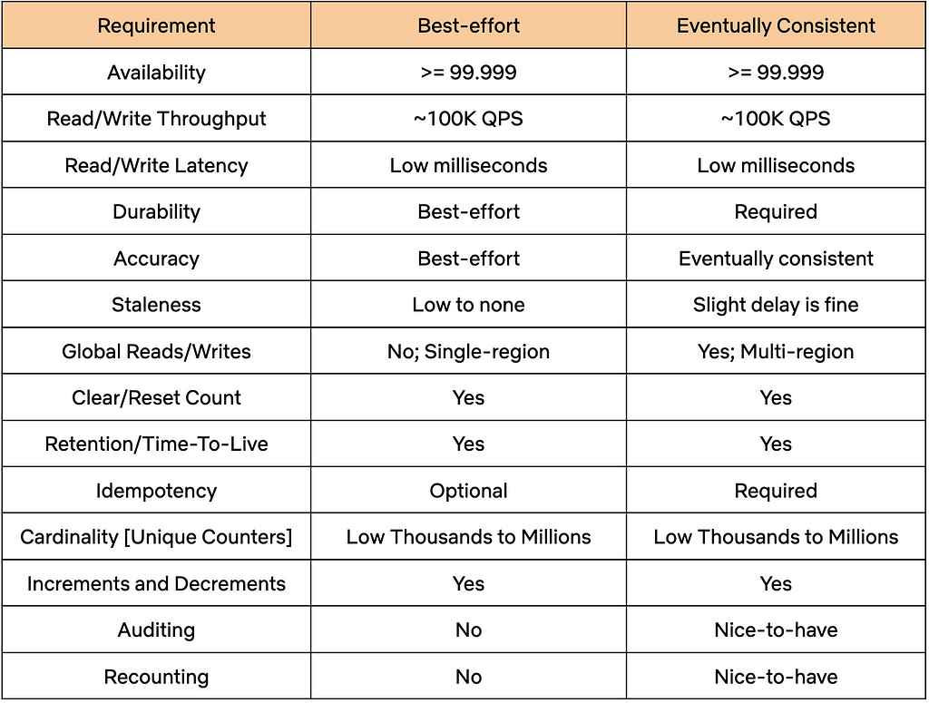
At Netflix, these use cases can be classified into two broad categories:
Best-Effort: For this category, the count doesn’t have to be very accurate or durable. However, this category requires near-immediate access to the current count at low latencies, all while keeping infrastructure costs to a minimum.
Eventually Consistent: This category needs accurate and durable counts, and is willing to tolerate a slight delay in accuracy and a slightly higher infrastructure cost as a trade-off.
Both categories share common requirements, such as high throughput and high availability. The table below provides a detailed overview of the diverse requirements across these two categories.
Distributed Counter Abstraction
To meet the outlined requirements, the Counter Abstraction was designed to be highly configurable. It allows users to choose between different counting modes, such as Best-Effort or Eventually Consistent, while considering the documented trade-offs of each option. After selecting a mode, users can interact with APIs without needing to worry about the underlying storage mechanisms and counting methods.
Let’s take a closer look at the structure and functionality of the API.
API
Counters are organized into separate namespaces that users set up for each of their specific use cases. Each namespace can be configured with different parameters, such as Type of Counter, Time-To-Live (TTL), and Counter Cardinality, using the service’s Control Plane.
The Counter Abstraction API resembles Java’s AtomicInteger interface:
AddCount/AddAndGetCount: Adjusts the count for the specified counter by the given delta value within a dataset. The delta value can be positive or negative. The AddAndGetCount counterpart also returns the count after performing the add operation.
The idempotency token can be used for counter types that support them. Clients can use this token to safely retry or hedge their requests. Failures in a distributed system are a given, and having the ability to safely retry requests enhances the reliability of the service.
GetCount: Retrieves the count value of the specified counter within a dataset.
Now, let’s look at the different types of counters supported within the Abstraction.
Types of Counters
The service primarily supports two types of counters: Best-Effort and Eventually Consistent, along with a third experimental type: Accurate. In the following sections, we’ll describe the different approaches for these types of counters and the trade-offs associated with each.
Best Effort Regional Counter
This type of counter is powered by EVCache, Netflix’s distributed caching solution built on the widely popular Memcached. It is suitable for use cases like A/B experiments, where many concurrent experiments are run for relatively short durations and an approximate count is sufficient. Setting aside the complexities of provisioning, resource allocation, and control plane management, the core of this solution is remarkably straightforward:
// clear counts from all replicas cache.delete(counterCacheKey, ReplicaPolicy.ALL);
EVCache delivers extremely high throughput at low millisecond latency or better within a single region, enabling a multi-tenant setup within a shared cluster, saving infrastructure costs. However, there are some trade-offs: it lacks cross-region replication for the increment operation and does not provide consistency guarantees, which may be necessary for an accurate count. Additionally, idempotency is not natively supported, making it unsafe to retry or hedge requests.
Edit: A note on probabilistic data structures:
Probabilistic data structures like HyperLogLog (HLL) can be useful for tracking an approximate number of distinct elements, like distinct views or visits to a website, but are not ideally suited for implementing distinct increments and decrements for a given key. Count-Min Sketch (CMS) is an alternative that can be used to adjust the values of keys by a given amount. Data stores like Redis support both HLL and CMS. However, we chose not to pursue this direction for several reasons:
We chose to build on top of data stores that we already operate at scale.
Probabilistic data structures do not natively support several of our requirements, such as resetting the count for a given key or having TTLs for counts. Additional data structures, including more sketches, would be needed to support these requirements.
On the other hand, the EVCache solution is quite simple, requiring minimal lines of code and using natively supported elements. However, it comes at the trade-off of using a small amount of memory per counter key.
Eventually Consistent Global Counter
While some users may accept the limitations of a Best-Effort counter, others opt for precise counts, durability and global availability. In the following sections, we’ll explore various strategies for achieving durable and accurate counts. Our objective is to highlight the challenges inherent in global distributed counting and explain the reasoning behind our chosen approach.
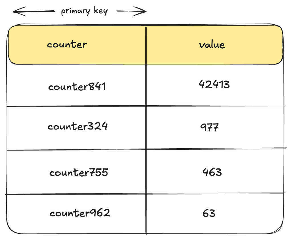
Approach 1: Storing a Single Row per Counter
Let’s start simple by using a single row per counter key within a table in a globally replicated datastore.
Let’s examine some of the drawbacks of this approach:
Lack of Idempotency: There is no idempotency key baked into the storage data-model preventing users from safely retrying requests. Implementing idempotency would likely require using an external system for such keys, which can further degrade performance or cause race conditions.
Heavy Contention: To update counts reliably, every writer must perform a Compare-And-Swap operation for a given counter using locks or transactions. Depending on the throughput and concurrency of operations, this can lead to significant contention, heavily impacting performance.
Secondary Keys: One way to reduce contention in this approach would be to use a secondary key, such as a bucket_id, which allows for distributing writes by splitting a given counter into buckets, while enabling reads to aggregate across buckets. The challenge lies in determining the appropriate number of buckets. A static number may still lead to contention with hot keys, while dynamically assigning the number of buckets per counter across millions of counters presents a more complex problem.
Let’s see if we can iterate on our solution to overcome these drawbacks.
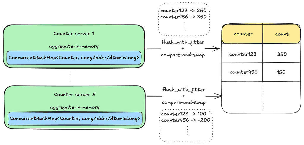
Approach 2: Per Instance Aggregation
To address issues of hot keys and contention from writing to the same row in real-time, we could implement a strategy where each instance aggregates the counts in memory and then flushes them to disk at regular intervals. Introducing sufficient jitter to the flush process can further reduce contention.
However, this solution presents a new set of issues:
Vulnerability to Data Loss: The solution is vulnerable to data loss for all in-memory data during instance failures, restarts, or deployments.
Inability to Reliably Reset Counts: Due to counting requests being distributed across multiple machines, it is challenging to establish consensus on the exact point in time when a counter reset occurred.
Lack of Idempotency: Similar to the previous approach, this method does not natively guarantee idempotency. One way to achieve idempotency is by consistently routing the same set of counters to the same instance. However, this approach may introduce additional complexities, such as leader election, and potential challenges with availability and latency in the write path.
That said, this approach may still be suitable in scenarios where these trade-offs are acceptable. However, let’s see if we can address some of these issues with a different event-based approach.
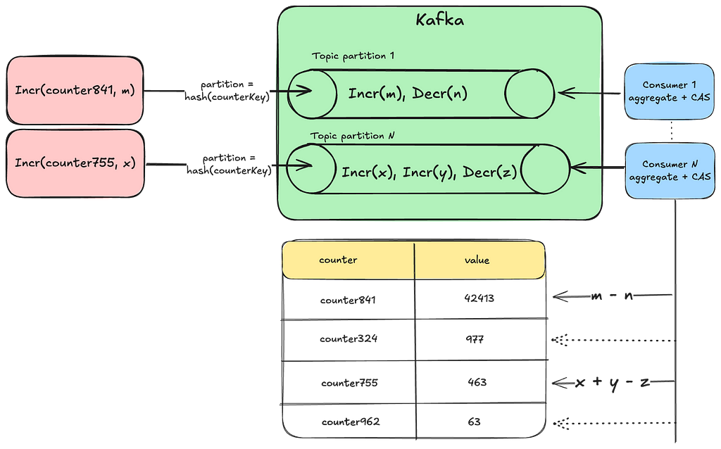
Approach 3: Using Durable Queues
In this approach, we log counter events into a durable queuing system like Apache Kafka to prevent any potential data loss. By creating multiple topic partitions and hashing the counter key to a specific partition, we ensure that the same set of counters are processed by the same set of consumers. This setup simplifies facilitating idempotency checks and resetting counts. Furthermore, by leveraging additional stream processing frameworks such as Kafka Streams or Apache Flink, we can implement windowed aggregations.
However, this approach comes with some challenges:
Potential Delays: Having the same consumer process all the counts from a given partition can lead to backups and delays, resulting in stale counts.
Rebalancing Partitions: This approach requires auto-scaling and rebalancing of topic partitions as the cardinality of counters and throughput increases.
Furthermore, all approaches that pre-aggregate counts make it challenging to support two of our requirements for accurate counters:
Auditing of Counts: Auditing involves extracting data to an offline system for analysis to ensure that increments were applied correctly to reach the final value. This process can also be used to track the provenance of increments. However, auditing becomes infeasible when counts are aggregated without storing the individual increments.
Potential Recounting: Similar to auditing, if adjustments to increments are necessary and recounting of events within a time window is required, pre-aggregating counts makes this infeasible.
Barring those few requirements, this approach can still be effective if we determine the right way to scale our queue partitions and consumers while maintaining idempotency. However, let’s explore how we can adjust this approach to meet the auditing and recounting requirements.
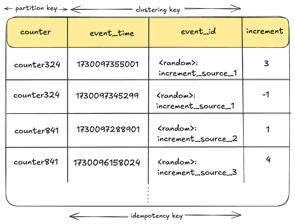
Approach 4: Event Log of Individual Increments
In this approach, we log each individual counter increment along with its event_time and event_id. The event_id can include the source information of where the increment originated. The combination of event_time and event_id can also serve as the idempotency key for the write.
However, in its simplest form, this approach has several drawbacks:
Read Latency: Each read request requires scanning all increments for a given counter potentially degrading performance.
Duplicate Work: Multiple threads might duplicate the effort of aggregating the same set of counters during read operations, leading to wasted effort and subpar resource utilization.
Wide Partitions: If using a datastore like Apache Cassandra, storing many increments for the same counter could lead to a wide partition, affecting read performance.
Large Data Footprint: Storing each increment individually could also result in a substantial data footprint over time. Without an efficient data retention strategy, this approach may struggle to scale effectively.
The combined impact of these issues can lead to increased infrastructure costs that may be difficult to justify. However, adopting an event-driven approach seems to be a significant step forward in addressing some of the challenges we’ve encountered and meeting our requirements.
How can we improve this solution further?
Netflix’s Approach
We use a combination of the previous approaches, where we log each counting activity as an event, and continuously aggregate these events in the background using queues and a sliding time window. Additionally, we employ a bucketing strategy to prevent wide partitions. In the following sections, we’ll explore how this approach addresses the previously mentioned drawbacks and meets all our requirements.
Note: From here on, we will use the words “rollup” and “aggregate” interchangeably. They essentially mean the same thing, i.e., collecting individual counter increments/decrements and arriving at the final value.
TimeSeries Event Store:
We chose the TimeSeries Data Abstraction as our event store, where counter mutations are ingested as event records. Some of the benefits of storing events in TimeSeries include:
High-Performance: The TimeSeries abstraction already addresses many of our requirements, including high availability and throughput, reliable and fast performance, and more.
Reducing Code Complexity: We reduce a lot of code complexity in Counter Abstraction by delegating a major portion of the functionality to an existing service.
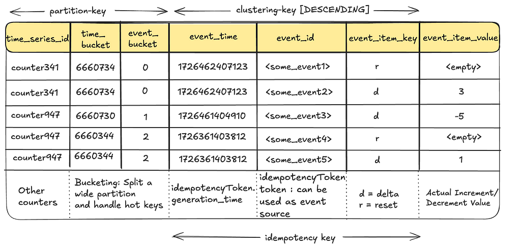
TimeSeries Abstraction uses Cassandra as the underlying event store, but it can be configured to work with any persistent store. Here is what it looks like:
Handling Wide Partitions: The time_bucket and event_bucket columns play a crucial role in breaking up a wide partition, preventing high-throughput counter events from overwhelming a given partition. For more information regarding this, refer to our previous blog.
No Over-Counting: The event_time, event_id and event_item_key columns form the idempotency key for the events for a given counter, enabling clients to retry safely without the risk of over-counting.
Event Ordering: TimeSeries orders all events in descending order of time allowing us to leverage this property for events like count resets.
Event Retention: The TimeSeries Abstraction includes retention policies to ensure that events are not stored indefinitely, saving disk space and reducing infrastructure costs. Once events have been aggregated and moved to a more cost-effective store for audits, there’s no need to retain them in the primary storage.
Now, let’s see how these events are aggregated for a given counter.
Aggregating Count Events:
As mentioned earlier, collecting all individual increments for every read request would be cost-prohibitive in terms of read performance. Therefore, a background aggregation process is necessary to continually converge counts and ensure optimal read performance.
But how can we safely aggregate count events amidst ongoing write operations?
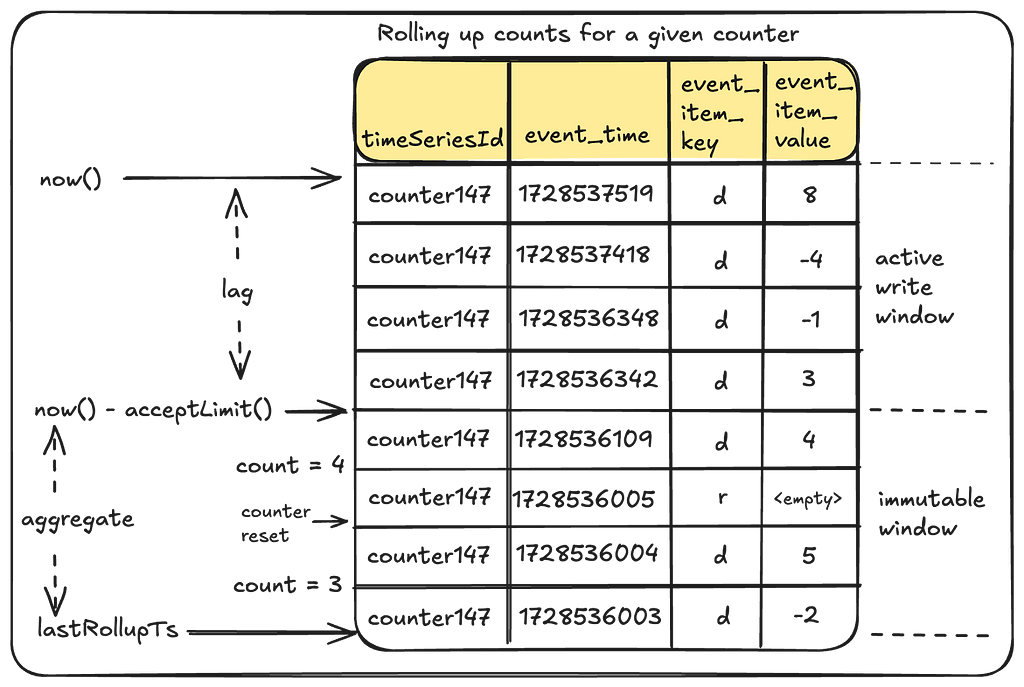
This is where the concept of Eventually Consistent counts becomes crucial. By intentionally lagging behind the current time by a safe margin, we ensure that aggregation always occurs within an immutable window.
Lets see what that looks like:
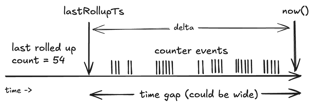
Let’s break this down:
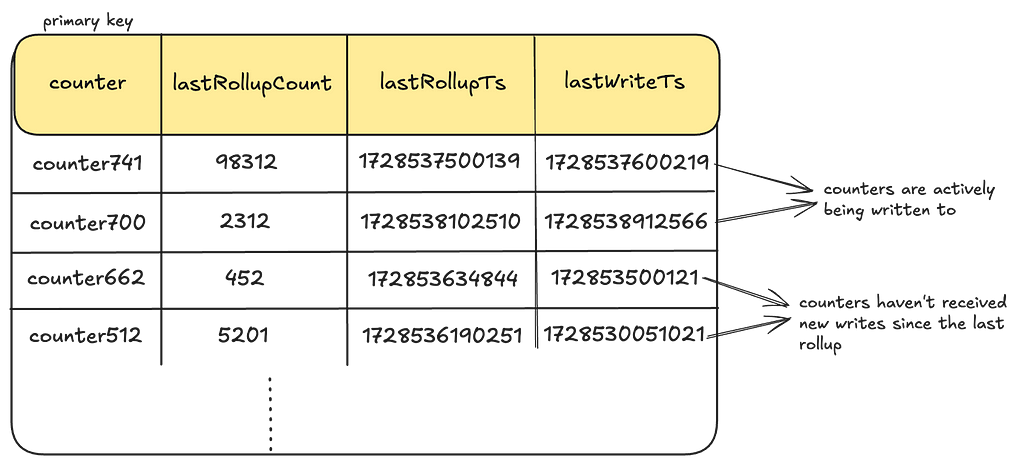
lastRollupTs: This represents the most recent time when the counter value was last aggregated. For a counter being operated for the first time, this timestamp defaults to a reasonable time in the past.
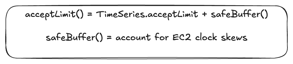
Immutable Window and Lag: Aggregation can only occur safely within an immutable window that is no longer receiving counter events. The “acceptLimit” parameter of the TimeSeries Abstraction plays a crucial role here, as it rejects incoming events with timestamps beyond this limit. During aggregations, this window is pushed slightly further back to account for clock skews.
This does mean that the counter value will lag behind its most recent update by some margin (typically in the order of seconds). This approach does leave the door open for missed events due to cross-region replication issues. See “Future Work” section at the end.
Aggregation Process: The rollup process aggregates all events in the aggregation window since the last rollup to arrive at the new value.
Rollup Store:
We save the results of this aggregation in a persistent store. The next aggregation will simply continue from this checkpoint.
We create one such Rollup table per dataset and use Cassandra as our persistent store. However, as you will soon see in the Control Plane section, the Counter service can be configured to work with any persistent store.
LastWriteTs: Every time a given counter receives a write, we also log a last-write-timestamp as a columnar update in this table. This is done using Cassandra’s USING TIMESTAMP feature to predictably apply the Last-Write-Win (LWW) semantics. This timestamp is the same as the event_time for the event. In the subsequent sections, we’ll see how this timestamp is used to keep some counters in active rollup circulation until they have caught up to their latest value.
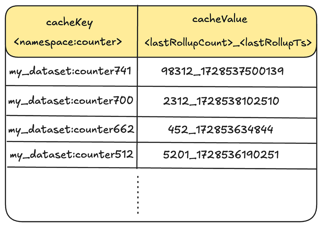
Rollup Cache
To optimize read performance, these values are cached in EVCache for each counter. We combine the lastRollupCount and lastRollupTsinto a single cached value per counter to prevent potential mismatches between the count and its corresponding checkpoint timestamp.
But, how do we know which counters to trigger rollups for? Let’s explore our Write and Read path to understand this better.
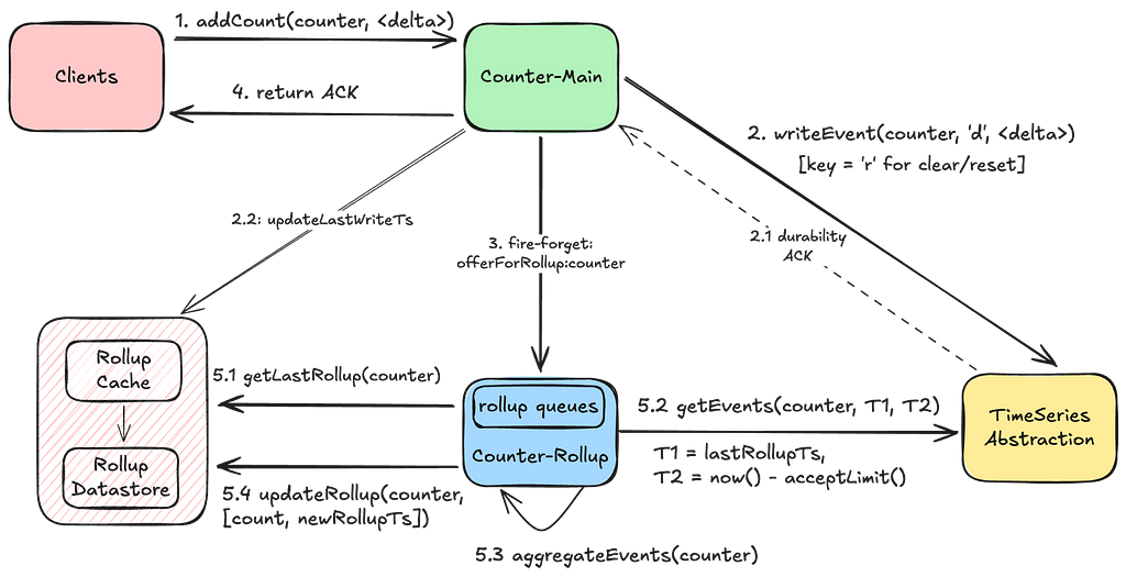
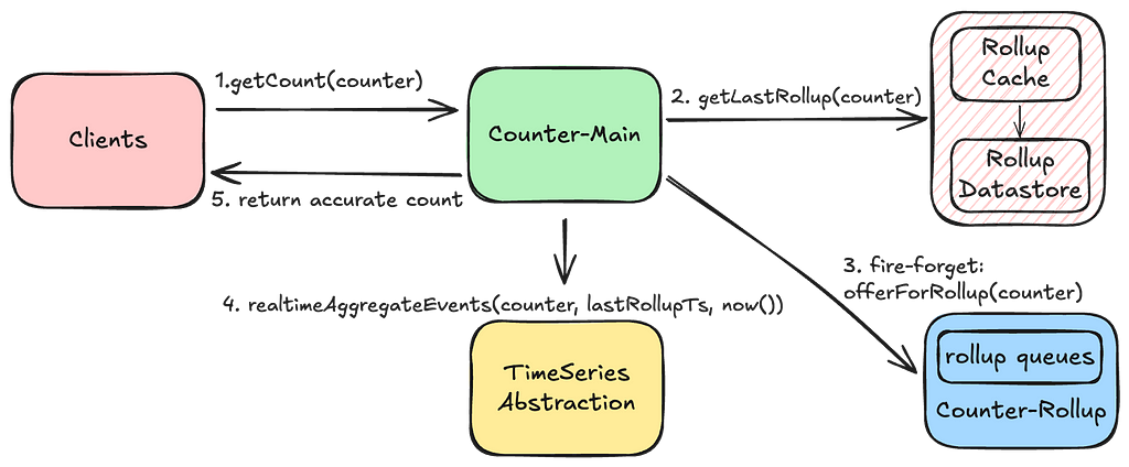
Add/Clear Count:
An add or clear count request writes durably to the TimeSeries Abstraction and updates the last-write-timestamp in the Rollup store. If the durability acknowledgement fails, clients can retry their requests with the same idempotency token without the risk of overcounting.Upon durability, we send a fire-and-forget request to trigger the rollup for the request counter.
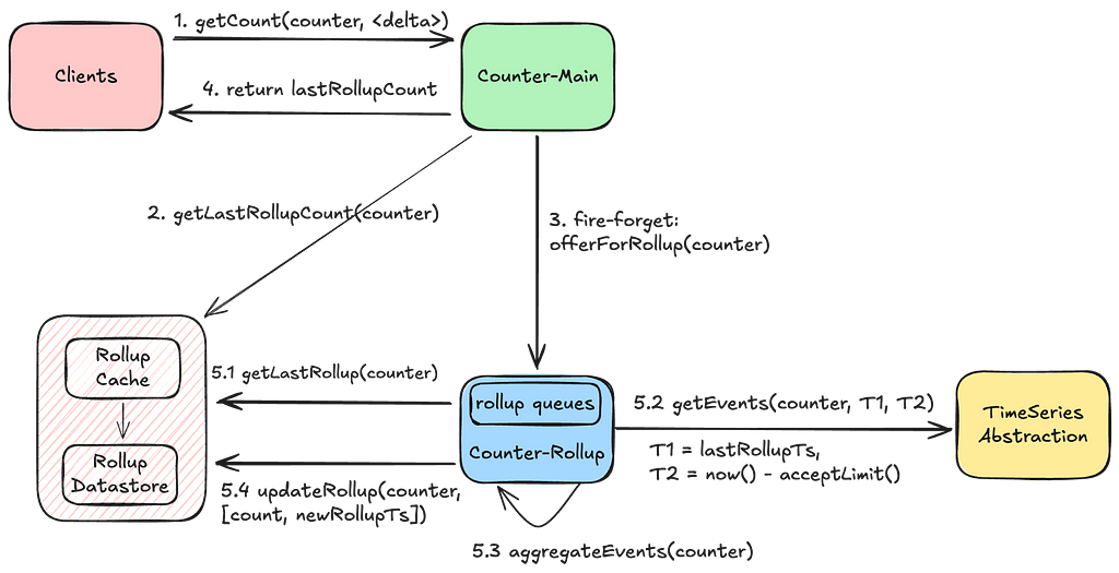
GetCount:
We return the last rolled-up count as a quick point-read operation, accepting the trade-off of potentially delivering a slightly stale count. We also trigger a rollup during the read operation to advance the last-rollup-timestamp, enhancing the performance of subsequent aggregations. This process also self-remediates a stale count if any previous rollups had failed.
With this approach, the counts continually converge to their latest value. Now, let’s see how we scale this approach to millions of counters and thousands of concurrent operations using our Rollup Pipeline.
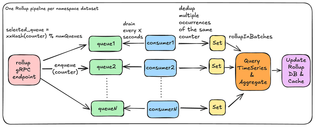
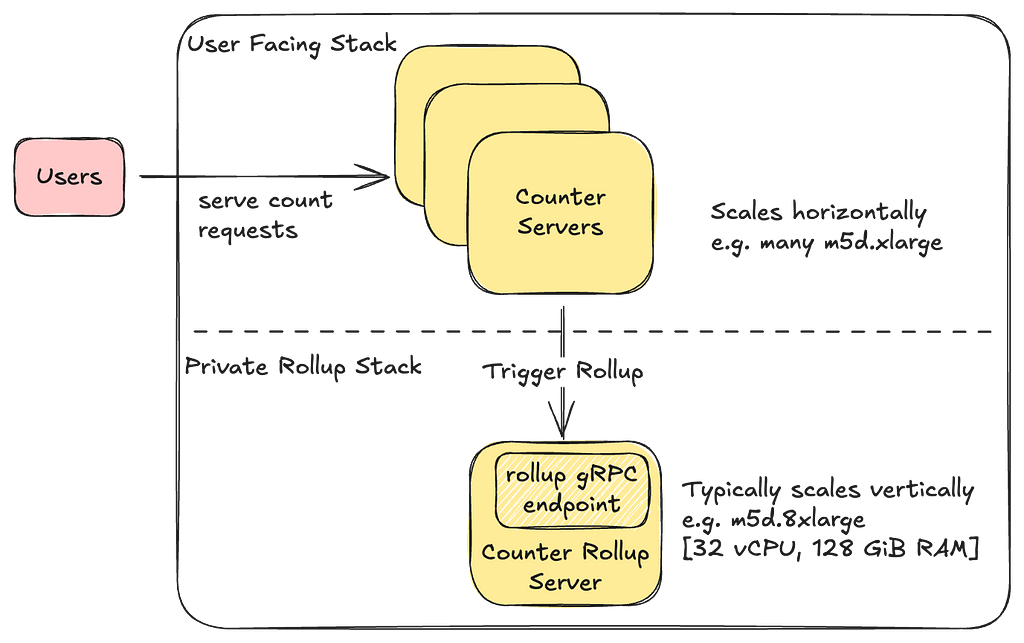
Rollup Pipeline:
Each Counter-Rollup server operates a rollup pipeline to efficiently aggregate counts across millions of counters. This is where most of the complexity in Counter Abstraction comes in. In the following sections, we will share key details on how efficient aggregations are achieved.
Light-Weight Roll-Up Event: As seen in our Write and Read paths above, every operation on a counter sends a light-weight event to the Rollup server:
Note that this event does not include the increment. This is only an indication to the Rollup server that this counter has been accessed and now needs to be aggregated. Knowing exactly which specific counters need to be aggregated prevents scanning the entire event dataset for the purpose of aggregations.
In-Memory Rollup Queues: A given Rollup server instance runs a set of in-memory queues to receive rollup events and parallelize aggregations. In the first version of this service, we settled on using in-memory queues to reduce provisioning complexity, save on infrastructure costs, and make rebalancing the number of queues fairly straightforward. However, this comes with the trade-off of potentially missing rollup events in case of an instance crash. For more details, see the “Stale Counts” section in “Future Work.”
Minimize Duplicate Effort: We use a fast non-cryptographic hash like XXHash to ensure that the same set of counters end up on the same queue. Further, we try to minimize the amount of duplicate aggregation work by having a separate rollup stack that chooses to run fewerbeefier instances.
Availability and Race Conditions: Having a single Rollup server instance can minimize duplicate aggregation work but may create availability challenges for triggering rollups. If we choose to horizontally scale the Rollup servers, we allow threads to overwrite rollup values while avoiding any form of distributed locking mechanisms to maintain high availability and performance. This approach remains safe because aggregation occurs within an immutable window. Although the concept of now() may differ between threads, causing rollup values to sometimes fluctuate, the counts will eventually converge to an accurate value within each immutable aggregation window.
Rebalancing Queues: If we need to scale the number of queues, a simple Control Plane configuration update followed by a re-deploy is enough to rebalance the number of queues.
      "eventual_counter_config": {
          "queue_config": {
            "num_queues" : 8,  // change to 16 and re-deploy
...
Handling Deployments: During deployments, these queues shut down gracefully, draining all existing events first, while the new Rollup server instance starts up with potentially new queue configurations. There may be a brief period when both the old and new Rollup servers are active, but as mentioned before, this race condition is managed since aggregations occur within immutable windows.
Minimize Rollup Effort: Receiving multiple events for the same counter doesn’t mean rolling it up multiple times. We drain these rollup events into a Set, ensuring a given counter is rolled up only onceduring a rollup window.
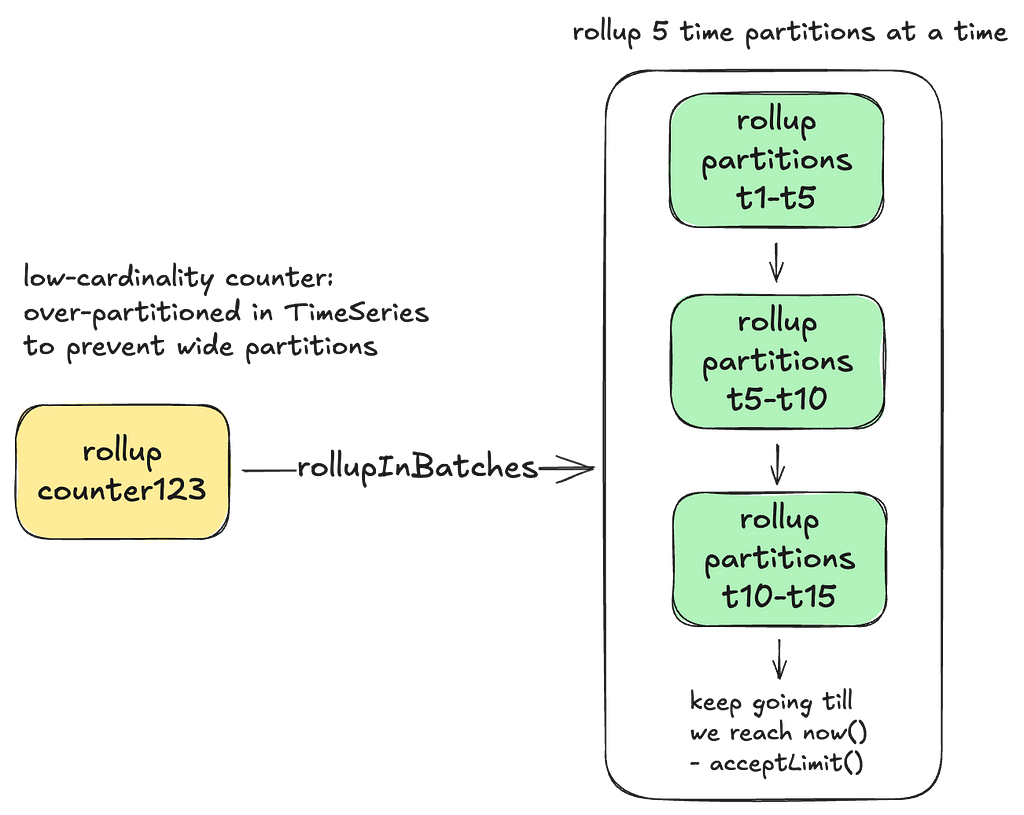
Efficient Aggregation: Each rollup consumer processes a batch of counters simultaneously. Within each batch, it queries the underlying TimeSeries abstraction in parallel to aggregate events within specified time boundaries. The TimeSeries abstraction optimizes these range scans to achieve low millisecond latencies.
Dynamic Batching: The Rollup server dynamically adjusts the number of time partitions that need to be scanned based on cardinality of counters in order to prevent overwhelming the underlying store with many parallel read requests.
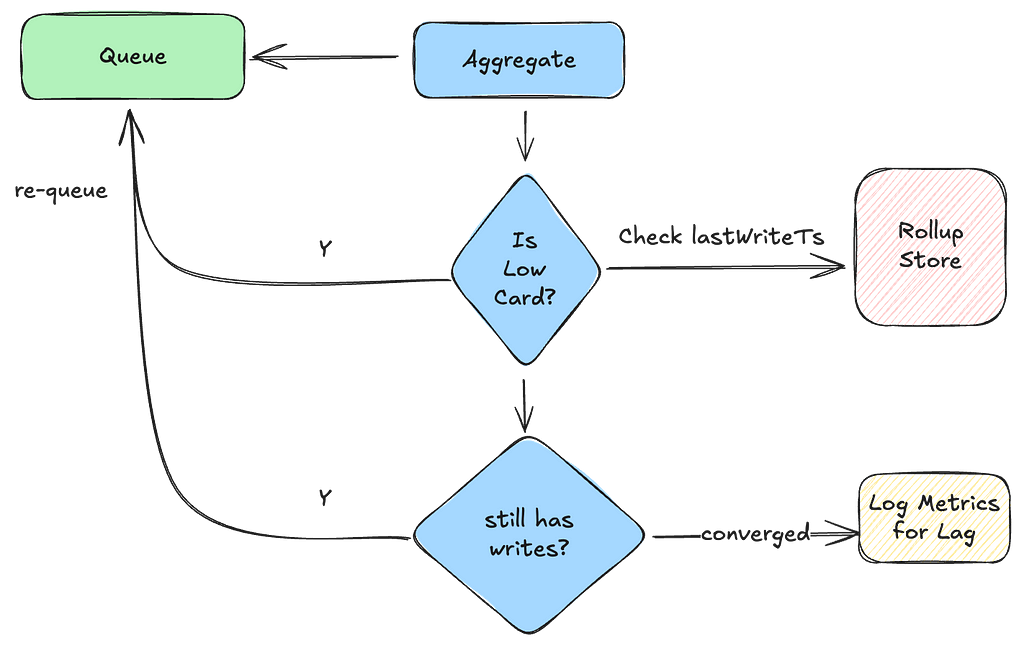
Adaptive Back-Pressure: Each consumer waits for one batch to complete before issuing the rollups for the next batch. It adjusts the wait time between batches based on the performance of the previous batch. This approach provides back-pressure during rollups to prevent overwhelming the underlying TimeSeries store.
Handling Convergence:
In order to prevent low-cardinality counters from lagging behind too much and subsequently scanning too many time partitions, they are kept in constant rollup circulation. For high-cardinality counters, continuously circulating them would consume excessive memory in our Rollup queues. This is where the last-write-timestamp mentioned previously plays a crucial role. The Rollup server inspects this timestamp to determine if a given counter needs to be re-queued, ensuring that we continue aggregating until it has fully caught up with the writes.
Now, let’s see how we leverage this counter type to provide an up-to-date current count in near-realtime.
Experimental: Accurate Global Counter
We are experimenting with a slightly modified version of the Eventually Consistent counter. Again, take the term ‘Accurate’ with a grain of salt. The key difference between this type of counter and its counterpart is that the delta, representing the counts since the last-rolled-up timestamp, is computed in real-time.
And then, currentAccurateCount = lastRollupCount + delta
Aggregating this delta in real-time can impact the performance of this operation, depending on the number of events and partitions that need to be scanned to retrieve this delta. The same principle of rolling up in batches applies here to prevent scanning too many partitions in parallel. Conversely, if the counters in this dataset areaccessedfrequently, the time gap for the delta remains narrow, making this approach of fetching current counts quite effective.
Now, let’s see how all this complexity is managed by having a unified Control Plane configuration.
Control Plane
The Data Gateway Platform Control Plane manages control settings for all abstractions and namespaces, including the Counter Abstraction. Below, is an example of a control plane configuration for a namespace that supports eventually consistent counters with low cardinality:
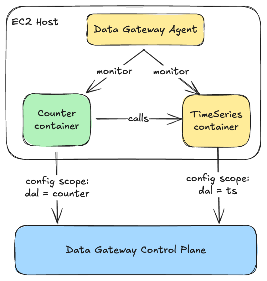
"persistence_configuration": [
  {
    "id": "CACHE",                             // Counter cache config
    "scope": "dal=counter",
    "physical_storage": {
      "type": "EVCACHE",                       // type of cache storage
      "cluster": "evcache_dgw_counter_tier1"   // Shared EVCache cluster
    }
  },
  {
    "id": "COUNTER_ROLLUP",
    "scope": "dal=counter",                    // Counter abstraction config
    "physical_storage": {
      "type": "CASSANDRA",                     // type of Rollup store
      "cluster": "cass_dgw_counter_uc1",       // physical cluster name
      "dataset": "my_dataset_1"                // namespace/dataset
    },
    "counter_cardinality": "LOW",              // supported counter cardinality
    "config": {
      "counter_type": "EVENTUAL",              // Type of counter
      "eventual_counter_config": {             // eventual counter type
        "internal_config": {
          "queue_config": {                    // adjust w.r.t cardinality
            "num_queues" : 8,                  // Rollup queues per instance
            "coalesce_ms": 10000,              // coalesce duration for rollups
            "capacity_bytes": 16777216         // allocated memory per queue
          },
          "rollup_batch_count": 32             // parallelization factor
        }
      }
    }
  },
  {
    "id": "EVENT_STORAGE",
    "scope": "dal=ts",                         // TimeSeries Event store
    "physical_storage": {
      "type": "CASSANDRA",                     // persistent store type
      "cluster": "cass_dgw_counter_uc1",       // physical cluster name
      "dataset": "my_dataset_1",               // keyspace name
    },
    "config": {
      "time_partition": {                      // time-partitioning for events
        "buckets_per_id": 4,                   // event buckets within
        "seconds_per_bucket": "600",           // smaller width for LOW card
        "seconds_per_slice": "86400",          // width of a time slice table
      },
      "accept_limit": "5s",                    // boundary for immutability
    },
    "lifecycleConfigs": {
      "lifecycleConfig": [
        {
          "type": "retention",                 // Event retention
          "config": {
            "close_after": "518400s",
            "delete_after": "604800s"          // 7 day count event retention
          }
        }
      ]
    }
  }
]
Using such a control plane configuration, we compose multiple abstraction layers using containers deployed on the same host, with each container fetching configuration specific to its scope.
Provisioning
As with the TimeSeries abstraction, our automation uses a bunch of user inputs regarding their workload and cardinalities to arrive at the right set of infrastructure and related control plane configuration. You can learn more about this process in a talk given by one of our stunning colleagues, Joey Lynch : How Netflix optimally provisions infrastructure in the cloud.
Performance
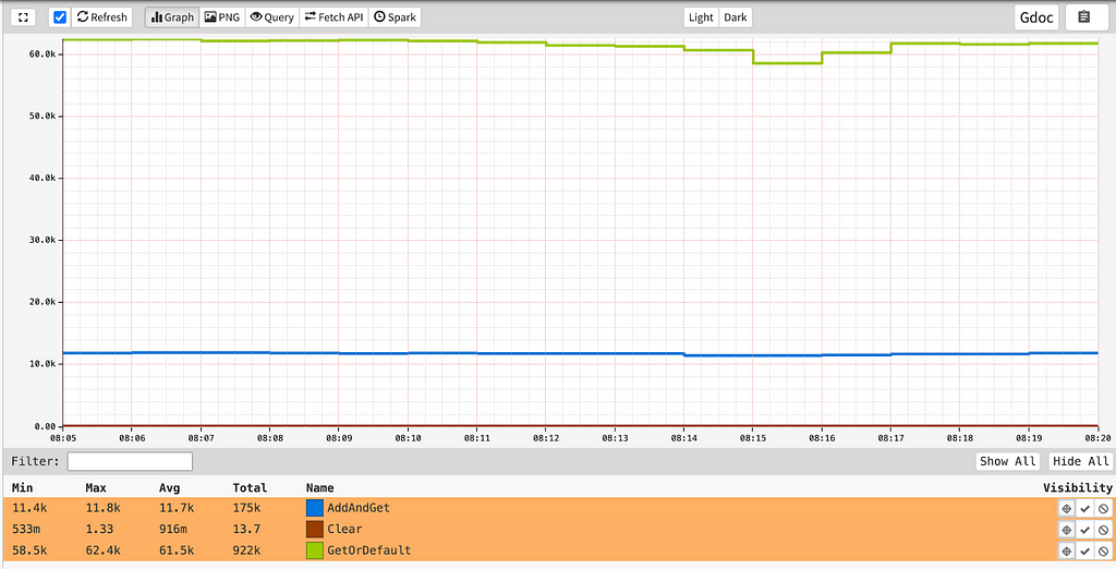
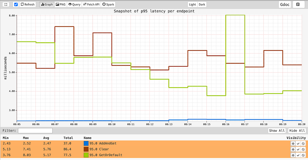
At the time of writing this blog, this service was processing close to 75K count requests/second globally across the different API endpoints and datasets:
while providing single-digit millisecond latencies for all its endpoints:
Future Work
While our system is robust, we still have work to do in making it more reliable and enhancing its features. Some of that work includes:
Regional Rollups: Cross-region replication issues can result in missed events from other regions. An alternate strategy involves establishing a rollup table for each region, and then tallying them in a global rollup table. A key challenge in this design would be effectively communicating the clearing of the counter across regions.
Error Detection and Stale Counts: Excessively stale counts can occur if rollup events are lost or if a rollup fails and isn’t retried. This isn’t an issue for frequently accessed counters, as they remain in rollup circulation. This issue is more pronounced for counters that aren’t accessed frequently. Typically, the initial read for such a counter will trigger a rollup, self-remediating the issue. However, for use cases that cannot accept potentially stale initial reads, we plan to implement improved error detection, rollup handoffs, and durable queues for resilient retries.
Conclusion
Distributed counting remains a challenging problem in computer science. In this blog, we explored multiple approaches to implement and deploy a Counting service at scale. While there may be other methods for distributed counting, our goal has been to deliver blazing fast performance at low infrastructure costs while maintaining high availability and providing idempotency guarantees. Along the way, we make various trade-offs to meet the diverse counting requirements at Netflix. We hope you found this blog post insightful.
Stay tuned for Part 3 of Composite Abstractions at Netflix, where we’ll introduce our Graph Abstraction, a new service being built on top of the Key-Value Abstractionand the TimeSeries Abstraction to handle high-throughput, low-latency graphs.
The authorization team at Netflix recently sponsored work to add Attribute Based Access Control (ABAC) support to AuthZed’s open source Google Zanzibar inspired authorization system, SpiceDB. Netflix required attribute support in SpiceDB to support core Netflix application identity constructs. This post discusses why Netflix wanted ABAC support in SpiceDB, how Netflix collaborated with AuthZed, the end result–SpiceDB Caveats, and how Netflix may leverage this new feature.
Netflix is always looking for security, ergonomic, or efficiency improvements, and this extends to authorization tools. Google Zanzibar is exciting to Netflix as it makes it easier to produce authorization decision objects and reverse indexes for resources a principal can access.
Last year, while experimenting with Zanzibar approaches to authorization, Netflix found SpiceDB, the open source Google Zanzibar inspired permission system, and built a prototype to experiment with modeling. The prototype uncovered trade-offs required to implement Attribute Based Access Control in SpiceDB, which made it poorly suited to Netflix’s core requirements for application identities.
Why did Netflix Want Caveated Relationships?
Netflix application identities are fundamentally attribute based: e.g. an instance of the Data Processor runs in eu-west-1 in the test environment with a public shard.
Authorizing these identities is done not only by application name, but by specifying specific attributes on which to match. An application owner might want to craft a policy like “Application members of the EU data processors group can access a PI decryption key”. This is one normal relationship in SpiceDB. But, they might also want to specify a policy for compliance reasons that only allows access to the PI key from data processor instances running in the EU within a sensitive shard. Put another way, an identity should only be considered to have the “is member of the EU-data-processors group” if certain identity attributes (like region==eu) match in addition to the application name. This is a Caveated SpiceDB relationship.
Netflix Modeling Challenges Before Caveats
SpiceDB, being a Relationship Based Access Control (ReBAC) system, expected authorization checks to be performed against the existence of a specific relationship between objects. Users fit this model — they have a single user ID to describe who they are. As described above, Netflix applications do not fit this model. Their attributes are used to scope permissions to varying degrees.
Netflix ran into significant difficulties in trying to fit their existing policy model into relations. To do so Netflix’s design required:
An event based mechanism that could ingest information about application autoscaling groups. An autoscaling group isn’t the lowest level of granularity, but it’s relatively close to the lowest level where we’d typically see authorization policy applied.
Ingest the attributes describing the autoscaling group and write them as separate relations. That is for the data-processor, Netflix would need to write relations describing the region, environment, account, application name, etc.
At authZ check time, provide the attributes for the identity to check, e.g. “can app bar in us-west-2 access this document.” SpiceDB is then responsible for figuring out which relations map back to the autoscaling group, e.g. name, environment, region, etc.
A cleanup process to prune stale relationships from the database.
What was problematic about this design? Aside from being complicated, there were a few specific things that made Netflix uncomfortable. The most salient being that it wasn’t resilient to an absence of relationship data, e.g. if a new autoscaling group started and reporting its presence to SpiceDB had not yet happened, the autoscaling group members would be missing necessary permissions to run. All this meant that Netflix would have to write and prune the relationship state with significant freshness requirements. This would be a significant departure from its existing policy based system.
While working through this, Netflix hopped into the SpiceDB Discord to chat about possible solutions and found an open community issue: the caveated relationships proposal.
The Beginning of SpiceDB Caveats
The SpiceDB community had already explored integrating SpiceDB with Open Policy Agent (OPA) and concluded it strayed too far from Zanzibar’s core promise of global horizontal scalability with strong consistency. With Netflix’s support, the AuthZed team pondered a Zanzibar-native approach to Attribute-Based Access Control.
The requirements were captured and published as the caveated relationships proposal on GitHub for feedback from the SpiceDB community. The community’s excitement and interest became apparent through comments, reactions, and conversations on the SpiceDB Discord server. Clearly, Netflix wasn’t the only one facing challenges when reconciling SpiceDB with policy-based approaches, so Netflix decided to help! By sponsoring the project, Netflix was able to help AuthZed prioritize engineering effort and accelerate adding Caveats to SpiceDB.
Building SpiceDB Caveats
Quick Intro to SpiceDB
The SpiceDB Schema Language lays the rules for how to build, traverse, and interpret SpiceDB’s Relationship Graph to make authorization decisions. SpiceDB Relationships, e.g., document:readme writer user:emilia, are stored as relationships that represent a graph within a datastore like CockroachDB or PostgreSQL. SpiceDB walks the graph and decomposes it into subproblems. These subproblems are assigned through consistent hashing and dispatched to a node in a cluster running SpiceDB. Over time, each node caches a subset of subproblems to support a distributed cache, reduce the datastore load, and achieve SpiceDB’s horizontal scalability.
SpiceDB Caveats Design
The fundamental challenge with policies is that their input arguments can change the authorization result as understood by a centralized relationships datastore. If SpiceDB were to cache subproblems that have been “tainted” with policy variables, the likelihood those are reused for other requests would decrease and thus severely affect the cache hit rate. As you’d suspect, this would jeopardize one of the pillars of the system: its ability to scale.
Once you accept that adding input arguments to the distributed cache isn’t efficient, you naturally gravitate toward the first question: what if you keep those inputs out of the cached subproblems? They are only known at request-time, so let’s add them as a variable in the subproblem! The cost of propagating those variables, assembling them, and executing the logic pales compared to fetching relationships from the datastore.
The next question was: how do you integrate the policy decisions into the relationships graph? The SpiceDB Schema Languages’ core concepts are Relations and Permissions; these are how a developer defines the shape of their relationships and how to traverse them. Naturally, being a graph, it’s fitting to add policy logic at the edges or the nodes. That leaves at least two obvious options: policy at the Relation level, or policy at the Permission level.
After iterating on both options to get a feel for the ergonomics and expressiveness the choice was policy at the relation level. After all, SpiceDB is a Relationship Based Access Control (ReBAC) system. Policy at the relation level allows you to parameterize each relationship, which brought about the saying “this relationship exists, but with a Caveat!.” With this approach, SpiceDB could do request-time relationship vetoing like so:
definition human {}

caveat the_answer(received int) {
  received == 42
}
definition the_answer_to_life_the_universe_and_everything {
  relation humans: human with the_answer
  permission enlightenment = humans
Netflix and AuthZed discussed the concept of static versus dynamic Caveats as well. A developer would define static Caveat expressions in the SpiceDB Schema, while dynamic Caveats would have expressions defined at run time. The discussion centered around typed versus dynamic programming languages, but given SpiceDB’s Schema Language was designed for type safety, it seemed coherent with the overall design to continue with static Caveats. To support runtime-provided policies, the choice was to introduce expressions as arguments to a Caveat. Keeping the SpiceDB Schema easy to understand was a key driver for this decision.
For defining Caveats, the main requirement was to provide an expression language with first-class support for partially-evaluated expressions. Google’s CEL seemed like the obvious choice: a protobuf-native expression language that evaluates in linear time, with first-class support for partial results that can be run at the edge, and is not turing complete. CEL expressions are type-safe, so they wouldn’t cause as many errors at runtime and can be stored in the datastore as a compiled protobuf. Given the near-perfect requirement match, it does make you wonder what Google’s Zanzibar has been up to since the white paper!
To execute the logic, SpiceDB would have to return a third response CAVEATED, in addition to ALLOW and DENY, to signal that a result of a CheckPermission request depends on computing an unresolved chain of CEL expressions.
SpiceDB Caveats needed to allow static input variables to be stored before evaluation to represent the multi-dimensional nature of Netflix application identities. Today, this is called “Caveat context,” defined by the values written in a SpiceDB Schema alongside a Relation and those provided by the client. Think of build time variables as an expansion of a templated CEL expression, and those take precedence over request-time arguments. Here is an example:
caveat the_answer(received int, expected int) {
  received == expected
}
Lastly, to deal with scenarios where there are multiple Caveated subproblems, the decision was to collect up a final CEL expression tree before evaluating it. The result of the final evaluation can be ALLOW, DENY, or CAVEATED. Things get trickier with wildcards and SpiceDB APIs, but let’s save that for another post! If the response is CAVEATED, the client receives a list of missing variables needed to properly evaluate the expression.
To sum up! The primary design decisions were:
Caveats defined at the Relation-level, not the Permission-level
Keep Caveats in line with SpiceDB Schema’s type-safe nature
Support well-typed values provided by the caller
Use Google’s CEL to define Caveat expressions
Introduce a new result type: CAVEATED
How do SpiceDB Caveats Change Authorizing Netflix Identities?
SpiceDB Caveats simplify this approach by allowing Netflix to specify authorization policy as they have in the past for applications. Instead of needing to have the entire state of the authorization world persisted as relations, the system can have relations and attributes of the identity used at authorization check time.
Now Netflix can write a Caveat similar to match_fine , described below, that takes lists of expected attributes, e.g. region, account, etc. This Caveat would allow the specific application named by the relation as long as the context of the authorization check had an observed account, stack, detail, region, and extended attribute values that matched the values in their expected counterparts. This playground has a live version of the schema, relations, etc. with which to experiment.
With the playground we can also make assertions that can mirror the behavior we’d see from the CheckPermission API. These assertions make it clear that our caveats work as expected.
Netflix and AuthZed are both excited about the collaboration’s outcome. Netflix has another authorization tool it can employ and SpiceDB users have another option with which to perform rich authorization checks. Bridging the gap between policy based authorization and ReBAC is a powerful paradigm that is already benefiting companies looking to Zanzibar based implementations for modernizing their authorization stack.
It’s hard to imagine a world without computer chips. They are at the heart of the devices that we use to work and play every day. Currently, Amazon Web Services (AWS) is offering customers the next generation of computer chip, with lower cost, higher performance, and a reduced carbon footprint.
This edition of Let’s Architect! focuses on custom computer chips, accelerators, and technologies developed by AWS, such as AWS Nitro System, custom-designed Arm-based AWS Graviton processors that support data-intensive workloads, as well as AWS Trainium, and AWS Inferentia chips optimized for machine learning training and inference.
In this post, we discuss these new AWS technologies, their main characteristics, and how to take advantage of them in your architecture.
As Deep Learning models become increasingly large and complex, the training cost for these models increases, as well as the inference time for serving.
With AWS Inferentia, machine learning practitioners can deploy complex neural-network models that are built and trained on popular frameworks, such as Tensorflow, PyTorch, and MXNet on AWS Inferentia-based Amazon EC2 Inf1 instances.
This video introduces you to the main concepts of AWS Inferentia, a service designed to reduce both cost and latency for inference. To speed up inference, AWS Inferentia: selects and shares a model across multiple chips, places pieces inside the on-chip cache, then streams the data via pipeline for low-latency predictions.
AWS Lambda is a serverless, event-driven compute service that enables code to run from virtually any type of application or backend service, without provisioning or managing servers. Lambda uses a high-availability compute infrastructure and performs all of the administration of the compute resources, including server- and operating-system maintenance, capacity-provisioning, and automatic scaling and logging.
AWS Graviton processors are designed to deliver the best price and performance for cloud workloads. AWS Graviton3 processors are the latest in the AWS Graviton processor family and provide up to: 25% increased compute performance, two-times higher floating-point performance, and two-times faster cryptographic workload performance compared with AWS Graviton2 processors. This means you can migrate AWS Lambda functions to Graviton in minutes, plus get as much as 19% improved performance at approximately 20% lower cost (compared with x86).
Comparison between x86 and Arm/Graviton2 results for the AWS Lambda function computing prime numbers (click to enlarge)
The AWS Nitro System is a collection of building-block technologies that includes AWS-built hardware offload and security components. It is powering the next generation of Amazon EC2 instances, with a broadening selection of compute, storage, memory, and networking options.
In this session, dive deep into the Nitro System, reviewing its design and architecture, exploring new innovations to the Nitro platform, and understanding how it allows for fasting innovation and increased security while reducing costs.
Traditionally, hypervisors protect the physical hardware and bios; virtualize the CPU, storage, networking; and provide a rich set of management capabilities. With the AWS Nitro System, AWS breaks apart those functions and offloads them to dedicated hardware and software.
AWS Nitro System separates functions and offloads them to dedicated hardware and software, in place of a traditional hypervisor
In this re:Invent 2021 session, we learn about the benefits Amazon’s ecommerce Datapath platform has realized with AWS Graviton.
With a range of 25%-40% performance gains across 53,000 Amazon EC2 instances worldwide for Prime Day 2021, the Datapath team is lowering their internal costs with AWS Graviton’s improved price performance. Explore the software updates that were required to achieve this and the testing approach used to optimize and validate the deployments. Finally, learn about the Datapath team’s migration approach that was used for their production deployment.
AWS Graviton2: core components
See you next time!
Thanks for exploring custom computer chips, accelerators, and technologies developed by AWS. Join us in a couple of weeks when we talk more about architectures and the daily challenges faced while working with distributed systems.
With the rapid growth in data coming from data platforms and applications, and the continuous improvements in state-of-the-art machine learning algorithms, data are becoming key assets for companies.
Modern data architectures include data mesh—a recent style that represents a paradigm shift, in which data is treated as a product and data architectures are designed around business domains. This type of approach supports the idea of distributed data, where each business domain focuses on the quality of the data it produces and exposes to the consumers.
In this edition of Let’s Architect!, we focus on data mesh and how it is designed on AWS, plus other approaches to adopt modern architectural patterns.
Domain Driven Design (DDD) is a software design approach where a solution is divided into domains aligned with business capabilities, software, and organizational boundaries. Unlike software architectures, most data architectures are often designed around technologies rather than business domains.
In this blog, you can learn about data mesh, an architectural pattern that applies the principles of DDD to data architectures. Data are organized into domains and considered the product that each team owns and offers for consumption.
A data mesh design organizes around data domains. Each domain owns multiple data products with their own data and technology stacks
In this video, discover how to use the data mesh approach in AWS. Specifically, how to implement certain design patterns for building a data mesh architecture with AWS services in the cloud.
This is a pragmatic presentation to get a quick understanding of data mesh fundamentals, the benefits/challenges, and the AWS services that you can use to build it. This video provides additional context to the aforementioned blog post and includes several examples on the benefits of modern data architectures.
This diagram demonstrates the pattern for sharing data catalogs between producer domains and consumer domains
In this blog, you can learn how to build a modern data strategy using AWS managed services to ingest data from sources like Salesforce. Also discussed is how to automatically create metadata catalogs and share data seamlessly between the data lake and data warehouse, plus creating alerts in the event of an orchestrated data workflow failure.
The second part of the post explains how a data warehouse can be built by using an agile data modeling pattern, as well as how ELT jobs were quickly developed, orchestrated, and configured to perform automated data quality testing.
A data platform architecture and the subcomponents used to build it
With a modern data architecture on AWS, architects and engineers can rapidly build scalable data lakes; use a broad and deep collection of purpose-built data services; and ensure compliance via unified data access, security, and governance. As data mesh is a modern architectural pattern, you can build it using a service like AWS Lake Formation.
Familiarize yourself with new technologies and services by not only learning how they work, but also to building prototypes and projects to gain hands-on experience. This workshop allows builders to become familiar with the features of AWS Lake Formation and its integrations with other AWS services.
A data catalog is a key component in a data mesh architecture. AWS Glue crawlers interact with data stores and other elements to populate the data catalog
See you next time!
Thanks for joining our discussion on data mesh! See you in a couple of weeks when we talk more about architectures and the challenges that we face every day while working with distributed systems.
AWS Architecture Center provides reference architecture diagrams, vetted architecture solutions, Well-Architected best practices, patterns, icons, and more!
The collective thoughts of the interwebz
Manage Consent
To provide the best experiences, we use technologies like cookies to store and/or access device information. Consenting to these technologies will allow us to process data such as browsing behavior or unique IDs on this site. Not consenting or withdrawing consent, may adversely affect certain features and functions.
Functional
Always active
The technical storage or access is strictly necessary for the legitimate purpose of enabling the use of a specific service explicitly requested by the subscriber or user, or for the sole purpose of carrying out the transmission of a communication over an electronic communications network.
Preferences
The technical storage or access is necessary for the legitimate purpose of storing preferences that are not requested by the subscriber or user.
Statistics
The technical storage or access that is used exclusively for statistical purposes.The technical storage or access that is used exclusively for anonymous statistical purposes. Without a subpoena, voluntary compliance on the part of your Internet Service Provider, or additional records from a third party, information stored or retrieved for this purpose alone cannot usually be used to identify you.
Marketing
The technical storage or access is required to create user profiles to send advertising, or to track the user on a website or across several websites for similar marketing purposes.