We want to be very careful with backward compatibility. We do not
want another Python 3 situation, so any changes in third-party code
needed to accommodate no-GIL builds should just work in with-GIL
builds (although backward compatibility with older Python versions
will still need to be addressed). This is not Python 4. We are
still considering the requirements we want to place on ABI
compatibility and other details for the two builds and the effect
on backward compatibility.
For those who are interested in the gory details of how the StackRot vulnerability works, Ruihan Li has
posted a detailed
writeup of the bug and how it can be exploited.
As StackRot is a Linux kernel vulnerability found in the memory
management subsystem, it affects almost all kernel configurations
and requires minimal capabilities to trigger. However, it should be
noted that maple nodes are freed using RCU callbacks, delaying the
actual memory deallocation until after the RCU grace
period. Consequently, exploiting this vulnerability is considered
challenging.
To the best of my knowledge, there are currently no publicly
available exploits targeting use-after-free-by-RCU (UAFBR)
bugs. This marks the first instance where UAFBR bugs have been
proven to be exploitable, even without the presence of
CONFIG_PREEMPT or CONFIG_SLAB_MERGE_DEFAULT settings.
We are introducing a new charge for public IPv4 addresses. Effective February 1, 2024 there will be a charge of $0.005 per IP per hour for all public IPv4 addresses, whether attached to a service or not (there is already a charge for public IPv4 addresses you allocate in your account but don’t attach to an EC2 instance).
Public IPv4 Charge As you may know, IPv4 addresses are an increasingly scarce resource and the cost to acquire a single public IPv4 address has risen more than 300% over the past 5 years. This change reflects our own costs and is also intended to encourage you to be a bit more frugal with your use of public IPv4 addresses and to think about accelerating your adoption of IPv6 as a modernization and conservation measure.
In-use Public IPv4 address (including Amazon provided public IPv4 and Elastic IP) assigned to resources in your VPC, Amazon Global Accelerator, and AWS Site-to-site VPN tunnel
The AWS Free Tier for EC2 will include 750 hours of public IPv4 address usage per month for the first 12 months, effective February 1, 2024. You will not be charged for IP addresses that you own and bring to AWS using Amazon BYOIP.
Starting today, your AWS Cost and Usage Reports automatically include public IPv4 address usage. When this price change goes in to effect next year you will also be able to use AWS Cost Explorer to see and better understand your usage.
Earlier this year we enhanced EC2 Instance Connect and gave it the ability to connect to your instances using private IPv4 addresses. As a result, you no longer need to use public IPv4 addresses for administrative purposes (generally using SSH or RDP).
Public IP Insights In order to make it easier for you to monitor, analyze, and audit your use of public IPv4 addresses, today we are launching Public IP Insights, a new feature of Amazon VPC IP Address Manager that is available to you at no cost. In addition to helping you to make efficient use of public IPv4 addresses, Public IP Insights will give you a better understanding of your security profile. You can see the breakdown of public IP types and EIP usage, with multiple filtering options:
You can also see, sort, filter, and learn more about each of the public IPv4 addresses that you are using:
Using IPv4 Addresses Efficiently By using the new IP Insights tool and following the guidance that I shared above, you should be ready to update your application to minimize the effect of the new charge. You may also want to consider using AWS Direct Connect to set up a dedicated network connection to AWS.
Apache Flink and Apache Spark are both open-source, distributed data processing frameworks used widely for big data processing and analytics. Spark is known for its ease of use, high-level APIs, and the ability to process large amounts of data. Flink shines in its ability to handle processing of data streams in real-time and low-latency stateful computations. Both support a variety of programming languages, scalable solutions for handling large amounts of data, and a wide range of connectors. Historically, Spark started out as a batch-first framework and Flink began as a streaming-first framework.
In this post, we share a comparative study of streaming patterns that are commonly used to build stream processing applications, how they can be solved using Spark (primarily Spark Structured Streaming) and Flink, and the minor variations in their approach. Examples cover code snippets in Python and SQL for both frameworks across three major themes: data preparation, data processing, and data enrichment. If you are a Spark user looking to solve your stream processing use cases using Flink, this post is for you. We do not intend to cover the choice of technology between Spark and Flink because it’s important to evaluate both frameworks for your specific workload and how the choice fits in your architecture; rather, this post highlights key differences for use cases that both these technologies are commonly considered for.
Apache Flink offers layered APIs that offer different levels of expressiveness and control and are designed to target different types of use cases. The three layers of API are Process Functions (also known as the Stateful Stream Processing API), DataStream, and Table and SQL. The Stateful Stream Processing API requires writing verbose code but offers the most control over time and state, which are core concepts in stateful stream processing. The DataStream API supports Java, Scala, and Python and offers primitives for many common stream processing operations, as well as a balance between code verbosity or expressiveness and control. The Table and SQL APIs are relational APIs that offer support for Java, Scala, Python, and SQL. They offer the highest abstraction and intuitive, SQL-like declarative control over data streams. Flink also allows seamless transition and switching across these APIs. To learn more about Flink’s layered APIs, refer to layered APIs.
Apache Spark Structured Streaming offers the Dataset and DataFrames APIs, which provide high-level declarative streaming APIs to represent static, bounded data as well as streaming, unbounded data. Operations are supported in Scala, Java, Python, and R. Spark has a rich function set and syntax with simple constructs for selection, aggregation, windowing, joins, and more. You can also use the Streaming Table API to read tables as streaming DataFrames as an extension to the DataFrames API. Although it’s hard to draw direct parallels between Flink and Spark across all stream processing constructs, at a very high level, we could say Spark Structured Streaming APIs are equivalent to Flink’s Table and SQL APIs. Spark Structured Streaming, however, does not yet (at the time of this writing) offer an equivalent to the lower-level APIs in Flink that offer granular control of time and state.
Both Flink and Spark Structured Streaming (referenced as Spark henceforth) are evolving projects. The following table provides a simple comparison of Flink and Spark capabilities for common streaming primitives (as of this writing).
.
Flink
Spark
Row-based processing
Yes
Yes
User-defined functions
Yes
Yes
Fine-grained access to state
Yes, via DataStream and low-level APIs
No
Control when state eviction occurs
Yes, via DataStream and low-level APIs
No
Flexible data structures for state storage and querying
Yes, via DataStream and low-level APIs
No
Timers for processing and stateful operations
Yes, via low level APIs
No
In the following sections, we cover the greatest common factors so that we can showcase how Spark users can relate to Flink and vice versa. To learn more about Flink’s low-level APIs, refer to Process Function. For the sake of simplicity, we cover the four use cases in this post using the Flink Table API. We use a combination of Python and SQL for an apples-to-apples comparison with Spark.
Data preparation
In this section, we compare data preparation methods for Spark and Flink.
Reading data
We first look at the simplest ways to read data from a data stream. The following sections assume the following schema for messages:
Note that we have to supply a schema object that captures our stock ticker schema (stock_ticker_schema). Compare this to the approach for Flink in the next section.
Reading data from a source using Flink Table API
For Flink, we use the SQL DDL statement CREATE TABLE. You can specify the schema of the stream just like you would any SQL table. The WITH clause allows us to specify the connector to the data stream (Kafka in this case), the associated properties for the connector, and data format specifications. See the following code:
JSON flattening is the process of converting a nested or hierarchical JSON object into a flat, single-level structure. This converts multiple levels of nesting into an object where all the keys and values are at the same level. Keys are combined using a delimiter such as a period (.) or underscore (_) to denote the original hierarchy. JSON flattening is useful when you need to work with a more simplified format. In both Spark and Flink, nested JSONs can be complicated to work with and may need additional processing or user-defined functions to manipulate. Flattened JSONs can simplify processing and improve performance due to reduced computational overhead, especially with operations like complex joins, aggregations, and windowing. In addition, flattened JSONs can help in easier debugging and troubleshooting data processing pipelines because there are fewer levels of nesting to navigate.
JSON flattening in Spark Structured Streaming
JSON flattening in Spark Structured Streaming requires you to use the select method and specify the schema that you need flattened. JSON flattening in Spark Structured Streaming involves specifying the nested field name that you’d like surfaced to the top-level list of fields. In the following example, company_info is a nested field and within company_info, there’s a field called company_name. With the following query, we’re flattening company_info.name to company_name:
In Flink SQL, you can use the JSON_VALUE function. Note that you can use this function only in Flink versions equal to or greater than 1.14. See the following code:
SELECT
   symbol,
   timestamp,
   price,
   JSON_VALUE(company_info, 'lax $.name' DEFAULT NULL ON EMPTY) AS company_name
FROM
   stock_ticker
The term lax in the preceding query has to do with JSON path expression handling in Flink SQL. For more information, refer to System (Built-in) Functions.
Data processing
Now that you have read the data, we can look at a few common data processing patterns.
Deduplication
Data deduplication in stream processing is crucial for maintaining data quality and ensuring consistency. It enhances efficiency by reducing the strain on the processing from duplicate data and helps with cost savings on storage and processing.
Spark Streaming deduplication query
The following code snippet is related to a Spark Streaming DataFrame named stock_ticker. The code performs an operation to drop duplicate rows based on the symbol column. The dropDuplicates method is used to eliminate duplicate rows in a DataFrame based on one or more columns.
The following code shows the Flink SQL equivalent to deduplicate data based on the symbol column. The query retrieves the first row for each distinct value in the symbol column from the stock_ticker stream, based on the ascending order of proctime:
SELECT symbol, timestamp, price
FROM (
  SELECT *,
    ROW_NUMBER() OVER (PARTITION BY symbol ORDER BY proctime ASC) AS row_num
  FROM stock_ticker)
WHERE row_num = 1
Windowing
Windowing in streaming data is a fundamental construct to process data within specifications. Windows commonly have time bounds, number of records, or other criteria. These time bounds bucketize continuous unbounded data streams into manageable chunks called windows for processing. Windows help in analyzing data and gaining insights in real time while maintaining processing efficiency. Analyses or operations are performed on constantly updating streaming data within a window.
There are two common time-based windows used both in Spark Streaming and Flink that we will detail in this post: tumbling and sliding windows. A tumbling window is a time-based window that is a fixed size and doesn’t have any overlapping intervals. A sliding window is a time-based window that is a fixed size and moves forward in fixed intervals that can be overlapping.
Spark Streaming tumbling window query
The following is a Spark Streaming tumbling window query with a window size of 10 minutes:
stock_ticker = ...  # Streaming DataFrame w/ schema shown above

# Get max stock price in tumbling window
# of size 10 minutes
visitsByWindowAndUser = visits
   .withWatermark("timestamp", "3 minutes")
   .groupBy(
      window(stock_ticker.timestamp, "10 minutes"),
      stock_ticker.symbol)
   .max(stock_ticker.price)
Flink Streaming tumbling window query
The following is an equivalent tumbling window query in Flink with a window size of 10 minutes:
SELECT symbol, MAX(price)
  FROM TABLE(
    TUMBLE(TABLE stock_ticker, DESCRIPTOR(timestamp), INTERVAL '10' MINUTES))
  GROUP BY ticker;
Spark Streaming sliding window query
The following is a Spark Streaming sliding window query with a window size of 10 minutes and slide interval of 5 minutes:
stock_ticker = ...  # Streaming DataFrame w/ schema shown above

# Get max stock price in sliding window
# of size 10 minutes and slide interval of size
# 5 minutes

visitsByWindowAndUser = visits
   .withWatermark("timestamp", "3 minutes")
   .groupBy(
      window(stock_ticker.timestamp, "10 minutes", "5 minutes"),
      stock_ticker.symbol)
   .max(stock_ticker.price)
Flink Streaming sliding window query
The following is a Flink sliding window query with a window size of 10 minutes and slide interval of 5 minutes:
SELECT symbol, MAX(price)
  FROM TABLE(
    HOP(TABLE stock_ticker, DESCRIPTOR(timestamp), INTERVAL '5' MINUTES, INTERVAL '10' MINUTES))
  GROUP BY ticker;
Handling late data
Both Spark Structured Streaming and Flink support event time processing, where a field within the payload can be used for defining time windows as distinct from the wall clock time of the machines doing the processing. Both Flink and Spark use watermarking for this purpose.
Watermarking is used in stream processing engines to handle delays. A watermark is like a timer that sets how long the system can wait for late events. If an event arrives and is within the set time (watermark), the system will use it to update a request. If it’s later than the watermark, the system will ignore it.
In the preceding windowing queries, you specify the lateness threshold in Spark using the following code:
.withWatermark("timestamp", "3 minutes")
This means that any records that are 3 minutes late as tracked by the event time clock will be discarded.
In contrast, with the Flink Table API, you can specify an analogous lateness threshold directly in the DDL:
WATERMARK FOR timestamp AS timestamp - INTERVAL '3' MINUTE
Note that Flink provides additional constructs for specifying lateness across its various APIs.
Data enrichment
In this section, we compare data enrichment methods with Spark and Flink.
Calling an external API
Calling external APIs from user-defined functions (UDFs) is similar in Spark and Flink. Note that your UDF will be called for every record processed, which can result in the API getting called at a very high request rate. In addition, in production scenarios, your UDF code often gets run in parallel across multiple nodes, further amplifying the request rate.
For the following code snippets, let’s assume that the external API call entails calling the function:
response = my_external_api(request)
External API call in Spark UDF
The following code uses Spark:
class Predict(ScalarFunction):
def open(self, function_context):

with open("resources.zip/resources/model.pkl", "rb") as f:
self.model = pickle.load(f)

def eval(self, x):
return self.model.predict(x)
External API call in Flink UDF
For Flink, assume we define the UDF callExternalAPIUDF, which takes as input the ticker symbol symbol and returns enriched information about the symbol via a REST endpoint. We can then register and call the UDF as follows:
callExternalAPIUDF = udf(callExternalAPIUDF(), result_type=DataTypes.STRING())

SELECT
    symbol,
    callExternalAPIUDF(symbol) as enriched_symbol
FROM stock_ticker;
Flink UDFs provide an initialization method that gets run one time (as opposed to one time per record processed).
Note that you should use UDFs judiciously as an improperly implemented UDF can cause your job to slow down, cause backpressure, and eventually stall your stream processing application. It’s advisable to use UDFs asynchronously to maintain high throughput, especially for I/O-bound use cases or when dealing with external resources like databases or REST APIs. To learn more about how you can use asynchronous I/O with Apache Flink, refer to Enrich your data stream asynchronously using Amazon Kinesis Data Analytics for Apache Flink.
Conclusion
Apache Flink and Apache Spark are both rapidly evolving projects and provide a fast and efficient way to process big data. This post focused on the top use cases we commonly encountered when customers wanted to see parallels between the two technologies for building real-time stream processing applications. We’ve included samples that were most frequently requested at the time of this writing. Let us know if you’d like more examples in the comments section.
About the author
Deepthi Mohan is a Principal Product Manager on the Amazon Kinesis Data Analytics team.
Karthi Thyagarajan was a Principal Solutions Architect on the Amazon Kinesis team.
Amazon Athena is a serverless, interactive analytics service built on the Trino, PrestoDB, and Apache Spark open-source frameworks. You can use Athena to run SQL queries on petabytes of data stored on Amazon Simple Storage Service (Amazon S3) in widely used formats such as Parquet and open-table formats like Apache Iceberg, Apache Hudi, and Delta Lake. However, Athena also allows you to query data stored in 30 different data sources—in addition to Amazon S3—including relational, non-relational, and object stores running on premises or in other cloud environments.
In Athena, we refer to queries on non-Amazon S3 data sources as federated queries. These queries run on the underlying database, which means you can analyze the data without learning a new query language and without the need for separate extract, transform, and load (ETL) scripts to extract, duplicate, and prepare data for analysis.
Recently, Athena added support for creating and querying views on federated data sources to bring greater flexibility and ease of use to use cases such as interactive analysis and business intelligence reporting. Athena also updated its data connectors with optimizations that improve performance and reduce cost when querying federated data sources. The updated connectors use dynamic filtering and an expanded set of predicate pushdown optimizations to perform more operations in the underlying data source rather than in Athena. As a result, you get faster queries with less data scanned, especially on tables with millions to billions of rows of data.
In this post, we show how to create and query views on federated data sources in a data mesh architecture featuring data producers and consumers.
The term data mesh refers to a data architecture with decentralized data ownership. A data mesh enables domain-oriented teams with the data they need, emphasizes self-service, and promotes the notion of purpose-built data products. In a data mesh, data producers expose datasets to the organization and data consumers subscribe to and consume the data products created by producers. By distributing data ownership to cross-functional teams, a data mesh can foster a culture of collaboration, invention, and agility around data.
Let’s dive into the solution.
Solution overview
For this post, imagine a hypothetical ecommerce company that uses multiple data sources, each playing a different role:
In an S3 data lake, ecommerce records are stored in a table named Lineitems
Amazon ElastiCache for Redis stores Nations and ActiveOrders data, ensuring ultra-fast reads of operational data by downstream ecommerce systems
On Amazon Relational Database Service (Amazon RDS), MySQL is used to store data like email addresses and shipping addresses in the Orders, Customer, and Suppliers tables
For flexibility and low-latency reads and writes, an Amazon DynamoDB table holds Part and Partsupp data
We want to query these data sources in a data mesh design. In the following sections, we set up Athena data source connectors for MySQL, DynamoDB, and Redis, and then run queries that perform complex joins across these data sources. The following diagram depicts our data architecture.
As you proceed with this solution, note that you will create AWS resources in your account. We have provided you with an AWS CloudFormation template that defines and configures the required resources, including the sample MySQL database, S3 tables, Redis store, and DynamoDB table. The template also creates the AWS Glue database and tables, S3 bucket, Amazon S3 VPC endpoint, AWS Glue VPC endpoint, and other AWS Identity and Access Management (IAM) resources that are used in the solution.
The template is designed to demonstrate how to use federated views in Athena, and is not intended for production use without modification. Additionally, the template uses the us-east-1 Region and will not work in other Regions without modification. The template creates resources that incur costs while they are in use. Follow the cleanup steps at the end of this post to delete the resources and avoid unnecessary charges.
Prerequisites
Before you launch the CloudFormation stack, ensure you have the following prerequisites:
An AWS account that provides access to AWS services
An IAM user with an access key and secret key to configure the AWS Command Line Interface (AWS CLI), and permissions to create an IAM role, IAM policies, and stacks in AWS CloudFormation
Create resources with AWS CloudFormation
To get started, complete the following steps:
Choose Launch Stack:
Select I acknowledge that this template may create IAM resources.
The CloudFormation stack takes approximately 20–30 minutes to complete. You can monitor its progress on the AWS CloudFormation console. When status reads CREATE_COMPLETE, your AWS account will have the resources necessary to implement this solution.
Deploy connectors and connect to data sources
With our resources provisioned, we can begin to connect the dots in our data mesh. Let’s start by connecting the data sources created by the CloudFormation stack with Athena.
On the Athena console, choose Data sources in the navigation pane.
Choose Create data source.
For Data sources, select MySQL, then choose Next.
For Data source name, enter a name, such as mysql. The Athena connector for MySQL is an AWS Lambda function that was created for you by the CloudFormation template.
For Connection details, choose Select or enter a Lambda function.
Choose mysql, then choose Next.
Review the information and choose Create data source.
Return to the Data sources page and choose mysql.
On the connector details page, choose the link under Lambda function to access the Lambda console and inspect the function associated with this connector.
Return to the Athena query editor.
For Data source, choose mysql.
For Database, choose the sales database.
For Tables, you should see a listing of MySQL tables that are ready for you to query.
Repeat these steps to set up the connectors for DynamoDB and Redis.
After all four data sources are configured, we can see the data sources on the Data source drop-down menu. All other databases and tables, like the lineitem table, which is stored on Amazon S3, are defined in the AWS Glue Data Catalog and can be accessed by choosing AwsDataCatalog as the data source.
Analyze data with Athena
With our data sources configured, we are ready to start running queries and using federated views in a data mesh architecture. Let’s start by trying to find out how much profit was made on a given line of parts, broken out by supplier nation and year.
For such a query, we need to calculate, for each nation and year, the profit for parts ordered in each year that were filled by a supplier in each nation. Profit is defined as the sum of [(l_extendedprice*(1-l_discount)) - (ps_supplycost * l_quantity)] for all line items describing parts in the specified line.
Answering this question requires querying all four data sources—MySQL, DynamoDB, Redis, and Amazon S3—and is accomplished with the following SQL:
SELECT
    n_name nation,
	year(CAST(o_orderdate AS date)) as o_year,
	((l_extendedprice * (1 - l_discount)) - (CAST(ps_supplycost AS double) * l_quantity)) as amount
FROM
    awsdatacatalog.data_lake.lineitem,
    dynamo.default.part,
    dynamo.default.partsupp,
    mysql.sales.supplier,
    mysql.sales.orders,
    redis.redis.nation
WHERE
    ((s_suppkey = l_suppkey)
    AND (ps_suppkey = l_suppkey)
	AND (ps_partkey = l_partkey)
	AND (p_partkey = l_partkey)
	AND (o_orderkey = l_orderkey)
	AND (s_nationkey = CAST(Regexp_extract(_key_, '.*-(.*)', 1) AS int)))
Running this query on the Athena console produces the following result.
This query is fairly complex: it involves multiple joins and requires special knowledge of the correct way to calculate profit metrics that other end-users may not possess.
To simplify the analysis experience for those users, we can hide this complexity behind a view. For more information on using views with federated data sources, see Querying federated views.
Use the following query to create the view in the data_lake database under the AwsDataCatalog data source:
CREATE OR REPLACE VIEW "data_lake"."federated_view" AS
SELECT
    n_name nation,
	year(CAST(o_orderdate AS date)) as o_year,
	((l_extendedprice * (1 - l_discount)) - (CAST(ps_supplycost AS double) * l_quantity)) as amount
FROM
    awsdatacatalog.data_lake.lineitem,
    dynamo.default.part,
    dynamo.default.partsupp,
    mysql.sales.supplier,
    mysql.sales.orders,
    redis.redis.nation
WHERE
    ((s_suppkey = l_suppkey)
    AND (ps_suppkey = l_suppkey)
	AND (ps_partkey = l_partkey)
	AND (p_partkey = l_partkey)
	AND (o_orderkey = l_orderkey)
	AND (s_nationkey = CAST(Regexp_extract(_key_, '.*-(.*)', 1) AS int)))
Next, run a simple select query to validate the view was created successfully: SELECT * FROM federated_view limit 10
The result should be similar to our previous query.
With our view in place, we can perform new analyses to answer questions that would be challenging without the view due to the complex query syntax that would be required. For example, we can find the total profit by nation:
SELECT nation, sum(amount) AS total
from federated_view
GROUP BY nation
ORDER BY nation ASC
Your results should resemble the following screenshot.
As you now see, the federated view makes it simpler for end-users to run queries on this data. Users are free to query a view of the data, defined by a knowledgeable data producer, rather than having to first acquire expertise in each underlying data source. Because Athena federated queries are processed where the data is stored, with this approach, we avoid duplicating data from the source system, saving valuable time and cost.
Use federated views in a multi-user model
So far, we have satisfied one of the principles of a data mesh: we created a data product (federated view) that is decoupled from its originating source and is available for on-demand analysis by consumers.
Next, we take our data mesh a step further by using federated views in a multi-user model. To keep it simple, assume we have one producer account, the account we used to create our four data sources and federated view, and one consumer account. Using the producer account, we give the consumer account permission to query the federated view from the consumer account.
The following figure depicts this setup and our simplified data mesh architecture.
Follow these steps to share the connectors and AWS Glue Data Catalog resources from the producer, which includes our federated view, with the consumer account:
Share the data sources mysql, redis, dynamo, and data_lake with the consumer account. For instructions, refer to Sharing a data source in Account A with Account B. Note that Account A represents the producer and Account B represents the consumer. Make sure you use the same data source names from earlier when sharing data. This is necessary for the federated view to work in a cross-account model.
Next, share the producer account’s AWS Glue Data Catalog with the consumer account by following the steps in Cross-account access to AWS Glue data catalogs. For the data source name, use shared_federated_catalog.
Switch to the consumer account, navigate to the Athena console, and verify that you see federated_view listed under Views in the shared_federated_catalog Data Catalog and data_lake database.
Next, run a sample query on the shared view to see the query results.
Clean up
To clean up the resources created for this post, complete the following steps:
On the Amazon S3 console, empty the bucket athena-federation-workshop-<account-id>.
If you’re using the AWS CLI, delete the objects in the athena-federation-workshop-<account-id> bucket with the following code. Make sure you run this command on the correct bucket. aws s3 rm s3://athena-federation-workshop-<account-id> --recursive
On the AWS CloudFormation console or the AWS CLI, delete the stack athena-federated-view-blog.
Summary
In this post, we demonstrated the functionality of Athena federated views. We created a view spanning four different federated data sources and ran queries against it. We also saw how federated views could be extended to a multi-user data mesh and ran queries from a consumer account.
To take advantage of federated views, ensure you are using Athena engine version 3 and upgrade your data source connectors to the latest version available. For information on how to upgrade a connector, see Updating a data source connector.
About the Authors
Saurabh Bhutyani is a Principal Big Data Specialist Solutions Architect at AWS. He is passionate about new technologies. He joined AWS in 2019 and works with customers to provide architectural guidance for running scalable analytics solutions and data mesh architectures using AWS analytics services like Amazon EMR, Amazon Athena, AWS Glue, AWS Lake Formation, and Amazon DataZone.
Pathik Shah is a Sr. Big Data Architect on Amazon Athena. He joined AWS in 2015 and has been focusing in the big data analytics space since then, helping customers build scalable and robust solutions using AWS analytics services.
Amazon Redshift is a petabyte-scale, enterprise-grade cloud data warehouse service delivering the best price-performance. Today, tens of thousands of customers run business-critical workloads on Amazon Redshift to cost-effectively and quickly analyze their data using standard SQL and existing business intelligence (BI) tools.
Amazon Redshift now makes it easier for you to run queries in AWS data lakes by automatically mounting the AWS Glue Data Catalog. You no longer have to create an external schema in Amazon Redshift to use the data lake tables cataloged in the Data Catalog. Now, you can use your AWS Identity and Access Management (IAM) credentials or IAM role to browse the Glue Data Catalog and query data lake tables directly from Amazon Redshift Query Editor v2 or your preferred SQL editors.
This feature is now available in all AWS commercial and US Gov Cloud Regions where Amazon Redshift RA3, Amazon Redshift Serverless, and AWS Glue are available. To learn more about auto-mounting of the Data Catalog in Amazon Redshift, refer to Querying the AWS Glue Data Catalog.
Enabling easy analytics for everyone
Amazon Redshift is helping tens of thousands of customers manage analytics at scale. Amazon Redshift offers a powerful analytics solution that provides access to insights for users of all skill levels. You can take advantage of the following benefits:
It enables organizations to analyze diverse data sources, including structured, semi-structured, and unstructured data, facilitating comprehensive data exploration
With its high-performance processing capabilities, Amazon Redshift handles large and complex datasets, ensuring fast query response times and supporting real-time analytics
Amazon Redshift provides features like Multi-AZ (preview) and cross-Region snapshot copy for high availability and disaster recovery, and provides authentication and authorization mechanisms to make it reliable and secure
With features like Amazon Redshift ML, it democratizes ML capabilities across a variety of user personas
Integration with advanced analytical tools empowers you to apply sophisticated techniques and build predictive models
Scalability and elasticity allow for seamless expansion as data and workloads grow
Overall, Amazon Redshift empowers organizations to uncover valuable insights, enhance decision-making, and gain a competitive edge in today’s data-driven landscape.
Amazon Redshift Top Benefits
The new automatic mounting of the AWS Glue Data Catalog feature enables you to directly query AWS Glue objects in Amazon Redshift without the need to create an external schema for each AWS Glue database you want to query. With automatic mounting the Data Catalog, Amazon Redshift automatically mounts the cluster account’s default Data Catalog during boot or user opt-in as an external database, named awsdatacatalog.
Relevant use cases for automatic mounting of the AWS Glue Data Catalog feature
You can use tools like Amazon EMR to create new data lake schemas in various formats, such as Apache Hudi, Delta Lake, and Apache Iceberg (preview). However, when analysts want to run queries against these schemas, it requires administrators to create external schemas for each AWS Glue database in Amazon Redshift. You can now simplify this integration using automatic mounting of the AWS Glue Data Catalog.
The following diagram illustrates this architecture.
Solution overview
You can now use SQL clients like Amazon Redshift Query Editor v2 to browse and query awsdatacatalog. In Query Editor V2, to connect to the awsdatacatalog database, choose the following:
Provision resources with AWS CloudFormation to populate Data Catalog objects
In this post, we use an AWS Glue crawler to create the external table ny_pub stored in Apache Parquet format in the Amazon Simple Storage Service (Amazon S3) location s3://redshift-demos/data/NY-Pub/. In this step, we create the solution resources using AWS CloudFormation to create a stack named CrawlS3Source-NYTaxiData in either us-east-1 (use the yml download or launch stack) or us-west-2 (use the yml download or launch stack). Stack creation performs the following actions:
Creates the crawler NYTaxiCrawler along with the new IAM role AWSGlueServiceRole-RedshiftAutoMount
Creates automountdb as the AWS Glue database
When the stack is complete, perform the following steps:
On the AWS Glue console, under Data Catalog in the navigation pane, choose Crawlers.
Open NYTaxiCrawler and choose Run crawler.
After the crawler is complete, you can see a new table called ny_pub in the Data Catalog under the automountdb database.
Alternatively, you can follow the manual instructions from the Amazon Redshift labs to create the ny_pub table.
Connect with Redshift Serverless and query the Data Catalog as a federated user using Query Editor V2
In this section, we use an IAM role with principal tags to enable fine-grained federated authentication to Redshift Serverless to access auto-mounting AWS Glue objects.
Complete the following steps:
Create an IAM role and add following permissions. For this post, we add full AWS Glue, Amazon Redshift, and Amazon S3 permissions for demo purposes. In an actual production scenario, it’s recommended to apply more granular permissions.
On the Tags tab, create a tag with Key as RedshiftDbRoles and Value as automount.
In Query Editor V2, run the following SQL statement as an admin user to create a database role named automount:
Create role automount;
Grant usage privileges to the database role:
GRANT USAGE ON DATABASE awsdatacatalog to role automount;
Switch the role to automountrole by passing the account number and role name.
In the Query Editor v2, choose your Redshift Serverless endpoint (right-click) and choose Create connection.
For Authentication, select Federated user.
For Database, enter the database name you want to connect to.
Choose Create connection.
You’re now ready to explore and query the automatic mounting of the Data Catalog in Redshift Serverless.
Connect with Redshift provisioned cluster and query the Data Catalog using Query Editor V2
To connect with Redshift provisioned cluster and access the Data Catalog, make sure you have completed the steps in the preceding section. Then complete the following steps:
Connect to Redshift Query Editor V2 using the database user name and password authentication method. For example, connect to the dev database using the admin user and password.
In an editor tab, assuming the user is present in Amazon Redshift, run the following SQL statement to grant an IAM user access to the Data Catalog:
GRANT USAGE ON DATABASE awsdatacatalog to "IAMR:automountrole";
As an admin user, choose the Settings icon, choose Account settings, and select Authenticate with IAM credentials.
Choose Save.
Switch roles to automountrole by passing the account number and role name.
Create or edit the connection and use the authentication method Temporary credentials using your IAM identity.
You are ready to explore and query the automatic mounting of the Data Catalog in Amazon Redshift.
Discover the auto-mounted objects
This section illustrates the SHOW commands for discovery of auto-mounted objects. See the following code:
// Discovery of Glue databases at the schema level
SHOW SCHEMAS FROM DATABASE awsdatacatalog;

// Discovery of Glue tables
 Syntax: SHOW TABLES FROM SCHEMA awsdatacatalog.<glue_db_name>;
Example: SHOW TABLES FROM SCHEMA awsdatacatalog.automountdb;

// Disocvery of Glue table columns
 Syntax: SHOW COLUMNS FROM TABLE awsdatacatalog.<glue_db_name>.<glue_table_name>;
Example: SHOW COLUMNS FROM TABLE awsdatacatalog.automountdb.ny_pub;
Configure permissions on catalog resources using AWS Lake Formation
To maintain backward compatibility with AWS Glue, Lake Formation has the following initial security settings:
The Super permission is granted to the group IAMAllowedPrincipals on all existing Data Catalog resources
The Use only IAM access control setting is enabled for new Data Catalog resources
These settings effectively cause access to Data Catalog resources and Amazon S3 locations to be controlled solely by IAM policies. Individual Lake Formation permissions are not in effect.
In this step, we will configure permissions on catalog resources using AWS Lake Formation. Before you create the Data Catalog, you need to update the default settings of Lake Formation so that access to Data Catalog resources (databases and tables) is managed by Lake Formation permissions:
Federate with Redshift Serverless and query the Data Catalog using Query Editor V2 and a third-party SQL client
With Redshift Serverless, you can connect to awsdatacatalog from a third-party client as a federated user from any identity provider (IdP). In this section, we will configure permission on catalog resources for Federated IAM role in AWS Lake Formation. Using AWS Lake Formation with Redshift, currently permission can be applied on IAM user or IAM role level.
If the user doesn’t exist in Amazon Redshift, you may need to create the IAM user with the password disabled as shown in the following code and then grant usage on awsdatacatalog:
Update the IAM role used in the federation setup. In addition to the permissions added to the IAM role, you need to add AWS Glue permissions and Amazon S3 permissions to access objects from Amazon S3. For this post, we add full AWS Glue and AWS S3 permissions for demo purposes. In an actual production scenario, it’s recommended to apply more granular permissions.
Now you’re ready to connect to Redshift Serverless using the Query Editor V2 and federated login.
Use the SSO URL from Okta and log in to your Okta account with your user credentials. For this demo, we log in with user Ethan.
In the Query Editor v2, choose your Redshift Serverless instance (right-click) and choose Create connection.
For Authentication, select Federated user.
For Database, enter the database name you want to connect to.
Choose Create connection.
Run the command select current_user to validate that you are logged in as a federated user.
User Ethan will be able to explore and access awsdatacatalog data.
To connect Redshift Serverless with a third-party client, make sure you have followed all the previous steps.
The following screenshot shows that federated user ethan is able to query the awsdatacatalog tables using three-part notation:
Connect with Redshift provisioned cluster and query the Data Catalog as a federated user using third-party clients
With Redshift provisioned cluster, you can connect with awsdatacatalog from a third-party client as a federated user from any IdP.
To connect as a federated user with the Redshift provisioned cluster, you need to follow the steps in the previous section that detailed how to connect with Redshift Serverless and query the Data Catalog as a federated user using Query Editor V2 and a third-party SQL client.
There are additional changes required in IAM policy. Update the IAM policy with the following code to use the GetClusterCredentialsWithIAM API:
Use the latest Redshift JDBC driver because it only supports querying the auto-mounted Data Catalog table for federated users
For URL, enter jdbc:redshift:iam://<cluster endpoint>:<port>:<databasename>?groupfederation=true. For example, jdbc:redshift:iam://redshift-cluster-1.abdef0abc0ab.us-east-2.redshift.amazonaws.com:5439/dev?groupfederation=true.
In the preceding URL, groupfederation is a mandatory parameter that allows you to authenticate with the IAM credentials.
The following screenshot shows that federated user ethan is able to query the awsdatacatalog tables using three-part notation.
Connect and query the Data Catalog as an IAM user using third-party clients
In this section, we provide instructions to set up a SQL client to query the auto-mounted awsdatacatalog.
Use three-part notation to reference the awsdatacatalog table in your SELECT statement. The first part is the database name, the second part is the AWS Glue database name, and the third part is the AWS Glue table name:
SELECT * FROM awsdatacatalog.<aws-glue-db-name>.<aws-glue-table-name>;
You can perform various scenarios that read the Data Catalog data and populate Redshift tables.
For this post, we use SQLWorkbench/J as the SQL client to query the Data Catalog. To set up SQL Workbench/J, complete the following steps:
Create a new connection in SQL Workbench/J and choose Amazon Redshift as the driver.
Choose Manage drivers and add all the files from the downloaded AWS JDBC driver pack .zip file (remember to unzip the .zip file).
You must use the latest Redshift JDBC driver because it only supports querying the auto-mounted Data Catalog table.
For URL, enter jdbc:redshift:iam://<cluster endpoint>:<port>:<databasename>?profile=<profilename>&groupfederation=true. For example, jdbc:redshift:iam://redshift-cluster-1.abdef0abc0ab.us-east-2.redshift.amazonaws.com:5439/dev?profile=user2&groupfederation=true.
We are using profile-based credentials as an example. You can use any AWS profile or IAM credential-based authentication as per your requirement. For more information on IAM credentials, refer to Options for providing IAM credentials.
The following screenshot shows that IAM user johndoe is able to list the awsdatacatalog tables using the SHOW command.
The following screenshot shows that IAM user johndoe is able to query the awsdatacatalog tables using three-part notation:
If you get the following error while using groupfederation=true, you need to use the latest Redshift driver:
Something unusual has occurred to cause the driver to fail. Please report this exception:Authentication with plugin is not supported for group federation [SQL State=99999]
Clean up
Complete the following steps to clean up your resources:
Delete the IAM role automountrole.
Delete the CloudFormation stack CrawlS3Source-NYTaxiData to clean up the crawler NYTaxiCrawler, the automountdb database from the Data Catalog, and the IAM role AWSGlueServiceRole-RedshiftAutoMount.
Update the default settings of Lake Formation:
In the navigation pane, under Data catalog, choose Settings.
Select both access control options choose Save.
In the navigation pane, under Permissions, choose Administrative roles and tasks.
In the Database creators section, choose Grant.
Search for IAMAllowedPrincipals and select Create database permission.
Choose Grant.
Considerations
Note the following considerations:
The Data Catalog auto-mount provides ease of use to analysts or database users. The security setup (setting up the permissions model or data governance) is owned by account and database administrators.
To achieve fine-grained access control, build a permissions model in AWS Lake Formation.
If the permissions have to be maintained at the Redshift database level, leave the AWS Lake Formation default settings as is and then run grant/revoke in Amazon Redshift.
If you are using a third-party SQL editor, and your query tool does not support browsing of multiple databases, you can use the “SHOW“ commands to list your AWS Glue databases and tables. You can also query awsdatacatalog objects using three-part notation (SELECT * FROM awsdatacatalog.<aws-glue-db-name>.<aws-glue-table-name>;) provided you have access to the external objects based on the permission model.
Conclusion
In this post, we introduced the automatic mounting of AWS Glue Data Catalog, which makes it easier for customers to run queries in their data lakes. This feature streamlines data governance and access control, eliminating the need to create an external schema in Amazon Redshift to use the data lake tables cataloged in AWS Glue Data Catalog. We showed how you can manage permission on auto-mounted AWS Glue-based objects using Lake Formation. The permission model can be easily managed and organized by administrators, allowing database users to seamlessly access external objects they have been granted access to.
As we strive for enhanced usability in Amazon Redshift, we prioritize unified data governance and fine-grained access control. This feature minimizes manual effort while ensuring the necessary security measures for your organization are in place.
Maneesh Sharma is a Senior Database Engineer at AWS with more than a decade of experience designing and implementing large-scale data warehouse and analytics solutions. He collaborates with various Amazon Redshift Partners and customers to drive better integration.
Debu Panda is a Senior Manager, Product Management at AWS. He is an industry leader in analytics, application platform, and database technologies, and has more than 25 years of experience in the IT world.
Rohit Vashishtha is a Senior Analytics Specialist Solutions Architect at AWS based in Dallas, Texas. He has 17 years of experience architecting, building, leading, and maintaining big data platforms. Rohit helps customers modernize their analytic workloads using the breadth of AWS services and ensures that customers get the best price/performance with utmost security and data governance.
The GDPR (General Data Protection Regulation) right to be forgotten, also known as the right to erasure, gives individuals the right to request the deletion of their personally identifiable information (PII) data held by organizations. This means that individuals can ask companies to erase their personal data from their systems and any third parties with whom the data was shared. Organizations must comply with these requests provided that there are no legitimate grounds for retaining the personal data, such as legal obligations or contractual requirements.
Amazon Redshift is a fully managed, petabyte-scale data warehouse service in the cloud. It is designed for analyzing large volumes of data and performing complex queries on structured and semi-structured data. Many customers are looking for best practices to keep their Amazon Redshift analytics environment compliant and have an ability to respond to GDPR right to forgotten requests.
In this post, we discuss challenges associated with implementation and architectural patterns and actionable best practices for organizations to respond to the right to be forgotten request requirements of the GDPR for data stored in Amazon Redshift.
Who does GDPR apply to?
The GDPR applies to all organizations established in the EU and to organizations, whether or not established in the EU, that process the personal data of EU individuals in connection with either the offering of goods or services to data subjects in the EU or the monitoring of behavior that takes place within the EU.
The following are key terms we use when discussing the GDPR:
Data subject – An identifiable living person and resident in the EU or UK, on whom personal data is held by a business or organization or service provider
Processor – The entity that processes the data on the instructions of the controller (for example, AWS)
Controller – The entity that determines the purposes and means of processing personal data (for example, an AWS customer)
Personal data – Information relating to an identified or identifiable person, including names, email addresses, and phone numbers
Implementing the right to be forgotten can include the following challenges:
Data identification – One of the main challenges is identifying all instances of personal data across various systems, databases, and backups. Organizations need to have a clear understanding of where personal data is being stored and how it is processed to effectively fulfill the deletion requests.
Data dependencies – Personal data can be interconnected and intertwined with other data systems, making it challenging to remove specific data without impacting the integrity of functionality of other systems or processes. It requires careful analysis to identify data dependencies and mitigate any potential risks or disruptions.
Data replication and backups – Personal data can exist in multiple copies due to data replication and backups. Ensuring the complete removal of data from all these copies and backups can be challenging. Organizations need to establish processes to track and manage data copies effectively.
Legal obligations and exemptions – The right to be forgotten is not absolute and may be subject to legal obligations or exemptions. Organizations need to carefully assess requests, considering factors such as legal requirements, legitimate interests, freedom of expression, or public interest to determine if the request can be fulfilled or if any exceptions apply.
Data archiving and retention – Organizations may have legal or regulatory requirements to retain certain data for a specific period. Balancing the right to be forgotten with the obligation to retain data can be a challenge. Clear policies and procedures need to be established to manage data retention and deletion appropriately.
Architecture patterns
Organizations are generally required to respond to right to be forgotten requests within 30 days from when the individual submits a request. This deadline can be extended by a maximum of 2 months taking into account the complexity and the number of the requests, provided that the data subject has been informed about the reasons for the delay within 1 month of the receipt of the request.
The following sections discuss a few commonly referenced architecture patterns, best practices, and options supported by Amazon Redshift to support your data subject’s GDPR right to be forgotten request in your organization.
Data management and governance
Addressing the challenges mentioned requires a combination of technical, operational, and legal measures. Organizations need to develop robust data governance practices, establish clear procedures for handling deletion requests, and maintain ongoing compliance with GDPR regulations.
Large organizations usually have multiple Redshift environments, databases, and tables spread across multiple Regions and accounts. To successfully respond to a data subject’s requests, organizations should have a clear strategy to determine how data is forgotten, flagged, anonymized, or deleted, and they should have clear guidelines in place for data audits.
Data mapping involves identifying and documenting the flow of personal data in an organization. It helps organizations understand how personal data moves through their systems, where it is stored, and how it is processed. By creating visual representations of data flows, organizations can gain a clear understanding of the lifecycle of personal data and identify potential vulnerabilities or compliance gaps.
Note that putting a comprehensive data strategy in place is not in scope for this post.
Audit tracking
Organizations must maintain proper documentation and audit trails of the deletion process to demonstrate compliance with GDPR requirements. A typical audit control framework should record the data subject requests (who is the data subject, when was it requested, what data, approver, due date, scheduled ETL process if any, and so on). This will help with your audit requests and provide the ability to roll back in case of accidental deletions observed during the QA process. It’s important to maintain the list of users and systems who may get impacted during this process to ensure effective communication.
Data discovery and findability
Findability is an important step of the process. Organizations need to have mechanisms to find the data under consideration in an efficient and quick manner for timely response. The following are some patterns and best practices you can employ to find the data in Amazon Redshift.
Tagging
Consider tagging your Amazon Redshift resources to quickly identify which clusters and snapshots contain the PII data, the owners, the data retention policy, and so on. Tags provide metadata about resources at a glance. Redshift resources, such as namespaces, workgroups, snapshots, and clusters can be tagged. For more information about tagging, refer to Tagging resources in Amazon Redshift.
Naming conventions
As a part of the modeling strategy, name the database objects (databases, schemas, tables, columns) with an indicator that they contain PII so that they can be queried using system tables (for example, make a list of the tables and columns where PII data is involved). Identifying the list of tables and users or the systems that have access to them will help streamline the communication process. The following sample SQL can help you find the databases, schemas, and tables with a name that contains PII:
SELECT
pg_catalog.pg_namespace.nspname AS schema_name,
pg_catalog.pg_class.relname AS table_name,
pg_catalog.pg_attribute.attname AS column_name,
pg_catalog.pg_database.datname AS database_name
FROM
pg_catalog.pg_namespace
JOIN pg_catalog.pg_class ON pg_catalog.pg_namespace.oid = pg_catalog.pg_class.relnamespace
JOIN pg_catalog.pg_attribute ON pg_catalog.pg_class.oid = pg_catalog.pg_attribute.attrelid
JOIN pg_catalog.pg_database ON pg_catalog.pg_attribute.attnum > 0
WHERE
pg_catalog.pg_attribute.attname LIKE '%PII%';

SELECT datname
FROM pg_database
WHERE datname LIKE '%PII%';

SELECT table_schema, table_name, column_name
FROM information_schema.columns
WHERE column_name LIKE '%PII%'
Separate PII and non-PII
Whenever possible, keep the sensitive data in a separate table, database, or schema. Isolating the data in a separate database may not always be possible. However, you can separate the non-PII columns in a separate table, for example, Customer_NonPII and Customer_PII, and then join them with an unintelligent key. This helps identify the tables that contain non-PII columns. This approach is straightforward to implement and keeps non-PII data intact, which can be useful for analysis purposes. The following figure shows an example of these tables.
Flag columns
In the preceding tables, rows in bold are marked with Forgotten_flag=Yes. You can maintain a Forgotten_flag as a column with the default value as No and update this value to Yes whenever a request to be forgotten is received. Also, as a best practice from HIPAA, do a batch deletion once in a month. The downstream and upstream systems need to respect this flag and include this in their processing. This helps identify the rows that need to be deleted. For our example, we can use the following code:
Delete from Customer_PII where forgotten_flag=“Yes”
Use Master data management system
Organizations that maintain a master data management system maintain a golden record for a customer, which acts as a single version of truth from multiple disparate systems. These systems also contain crosswalks with several peripheral systems that contain the natural key of the customer and golden record. This technique helps find customer records and related tables. The following is a representative example of a crosswalk table in a master data management system.
Use AWS Lake Formation
Some organizations have use cases where you can share the data across multiple departments and business units and use Amazon Redshift data sharing. We can use AWS Lake Formation tags to tag the database objects and columns and define fine-grained access controls on who can have the access to use data. Organizations can have a dedicated resource with access to all tagged resources. With Lake Formation, you can centrally define and enforce database-, table-, column-, and row-level access permissions of Redshift data shares and restrict user access to objects within a data share.
By sharing data through Lake Formation, you can define permissions in Lake Formation and apply those permissions to data shares and their objects. For example, if you have a table containing employee information, you can use column-level filters to help prevent employees who don’t work in the HR department from seeing sensitive information. Refer to AWS Lake Formation-managed Redshift shares for more details on the implementation.
Use Amazon DataZone
Amazon DataZone introduces a business metadata catalog. Business metadata provides information authored or used by businesses and gives context to organizational data. Data discovery is a key task that business metadata can support. Data discovery uses centrally defined corporate ontologies and taxonomies to classify data sources and allows you to find relevant data objects. You can add business metadata in Amazon DataZone to support data discovery.
Data erasure
By using the approaches we’ve discussed, you can find the clusters, databases, tables, columns, snapshots that contain the data to be deleted. The following are some methods and best practices for data erasure.
Restricted backup
In some use cases, you may have to keep data backed up to align with government regulations for a certain period of time. It’s a good idea to take the backup of the data objects before deletion and keep it for an agreed-upon retention time. You can use AWS Backup to take automatic or manual backups. AWS Backup allows you to define a central backup policy to manage the data protection of your applications. For more information, refer to New – Amazon Redshift Support in AWS Backup.
Physical deletes
After we find the tables that contain the data, we can delete the data using the following code (using the flagging technique discussed earlier):
Delete from Customer_PII where forgotten_flag=“Yes”
It’s a good practice to delete data at a specified schedule, such as once every 25–30 days, so that it is simpler to maintain the state of the database.
Logical deletes
You may need to keep data in a separate environment for audit purposes. You can employ Amazon Redshift row access policies and conditional dynamic masking policies to filter and anonymize the data.
You can use conditional dynamic data masking policies so that designated users can see the redacted data. With dynamic data masking (DDM) in Amazon Redshift, organizations can help protect sensitive data in your data warehouse. You can manipulate how Amazon Redshift shows sensitive data to the user at query time without transforming it in the database. You control access to data through masking policies that apply custom obfuscation rules to a given user or role. That way, you can respond to changing privacy requirements without altering the underlying data or editing SQL queries.
Dynamic data masking policies hide, obfuscate, or pseudonymize data that matches a given format. When attached to a table, the masking expression is applied to one or more of its columns. You can further modify masking policies to only apply them to certain users or user-defined roles that you can create with role-based access control (RBAC). Additionally, you can apply DDM on the cell level by using conditional columns when creating your masking policy.
Organizations can use conditional dynamic data masking to redact sensitive columns (for example, names) where the forgotten flag column value is TRUE, and the other columns display the full values.
Backup and restore
Data from Redshift clusters can be transferred, exported, or copied to different AWS services or outside of the cloud. Organizations should have an effective governance process to detect and remove data to align with the GDPR compliance requirement. However, this is beyond the scope of this post.
Amazon Redshift offers backups and snapshots of the data. After deleting the PII data, organizations should also purge the data from their backups. To do so, you need to restore the snapshot to a new cluster, remove the data, and take a fresh backup. The following figure illustrates this workflow.
It’s good practice to keep the retention period at 29 days (if applicable) so that the backups are cleared after 30 days. Organizations can also set the backup schedule to a certain date (for example, the first of every month).
Communication
It’s important to communicate to the users and processes who may be impacted by this deletion. The following query helps identify the list of users and groups who have access to the affected tables:
SELECT
nspname AS schema_name,
relname AS table_name,
attname AS column_name,
usename AS user_name,
groname AS group_name
FROM pg_namespace
JOIN pg_class ON pg_namespace.oid = pg_class.relnamespace
JOIN pg_attribute ON pg_class.oid = pg_attribute.attrelid
LEFT JOIN pg_group ON pg_attribute.attacl::text LIKE '%' || groname || '%'
LEFT JOIN pg_user ON pg_attribute.attacl::text LIKE '%' || usename || '%'
WHERE
pg_attribute.attname LIKE '%PII%'
AND (usename IS NOT NULL OR groname IS NOT NULL);
Security controls
Maintaining security is of great importance in GDPR compliance. By implementing robust security measures, organizations can help protect personal data from unauthorized access, breaches, and misuse, thereby helping maintain the privacy rights of individuals. Security plays a crucial role in upholding the principles of confidentiality, integrity, and availability of personal data. AWS offers a comprehensive suite of services and features that can support GDPR compliance and enhance security measures.
The GDPR does not change the AWS shared responsibility model, which continues to be relevant for customers. The shared responsibility model is a useful approach to illustrate the different responsibilities of AWS (as a data processor or subprocessor) and customers (as either data controllers or data processors) under the GDPR.
Under the shared responsibility model, AWS is responsible for securing the underlying infrastructure that supports AWS services (“Security of the Cloud”), and customers, acting either as data controllers or data processors, are responsible for personal data they upload to AWS services (“Security in the Cloud”).
Article 32 of the GDPR requires that organizations must “…implement appropriate technical and organizational measures to ensure a level of security appropriate to the risk, including …the pseudonymization and encryption of personal data[…].” In addition, organizations must “safeguard against the unauthorized disclosure of or access to personal data.” Refer to the Navigating GDPR Compliance on AWS whitepaper for more details.
Conclusion
In this post, we delved into the significance of GDPR and its impact on safeguarding privacy rights. We discussed five commonly followed best practices that organizations can reference for responding to GDPR right to be forgotten requests for data that resides in Redshift clusters. We also highlighted that the GDPR does not change the AWS shared responsibility model.
We encourage you to take charge of your data privacy today. Prioritizing GPDR compliance and data privacy will not only strengthen trust, but also build customer loyalty and safeguard personal information in digital era. If you need assistance or guidance, reach out to an AWS representative. AWS has teams of Enterprise Support Representatives, Professional Services Consultants, and other staff to help with GDPR questions. You can contact us with questions. To learn more about GDPR compliance when using AWS services, refer to the General Data Protection Regulation (GDPR) Center. To learn more about the right to be forgotten, refer to Right to Erasure.
Disclaimer: The information provided above is not a legal advice. It is intended to showcase commonly followed best practices. It is crucial to consult with your organization’s privacy officer or legal counsel and determine appropriate solutions.
About the Authors
Yadukishore Tatavarthi is a Senior Partner Solutions Architect supporting Healthcare and life science customers at Amazon Web Services. He has been helping the customers over the last 20 years in building the enterprise data strategies, advising customers on cloud implementations, migrations, reference architecture creation, data modeling best practices, data lake/warehouses architecture, and other technical processes.
Sudhir Gupta is a Principal Partner Solutions Architect, Analytics Specialist at AWS with over 18 years of experience in Databases and Analytics. He helps AWS partners and customers design, implement, and migrate large-scale data & analytics (D&A) workloads. As a trusted advisor to partners, he enables partners globally on AWS D&A services, builds solutions/accelerators, and leads go-to-market initiatives
Deepak Singh is a Senior Solutions Architect at Amazon Web Services with 20+ years of experience in Data & AIA. He enjoys working with AWS partners and customers on building scalable analytical solutions for their business outcomes. When not at work, he loves spending time with family or exploring new technologies in analytics and AI space.
This week, community contributor h00die added an exploit module that leverages a command injection vulnerability in VMWare Aria Operations for Networks, formerly known as vRealize Network Insight. Versions 6.2 to 6.10 are vulnerable (CVE-2023-20887). A remote attacker could abuse the Apache Thrift RPC interface by sending specially crafted data and get unauthenticated remote code execution on the underlying operating system as the root user. The module first bypasses the reverse proxy that protects the RPC interface and executes its payload with root privileges. This vulnerability has been rated as critical by VMware, with a CVSSv3 base score of 9.8.
Again, WordPress Plugin
Community contributor h00die-gr3y added an exploit module that targets the File Manager Advanced Shortcode WordPress plugin. This module leverages a flaw in the data validation mechanism when uploading a file and gets unauthenticated remote code execution. The plugin does not correctly prevent uploading files with disallowed MIME types. This vulnerability is identified as CVE-2023-2068 and affects version 2.3.2 and prior.
Kerberos Authentication and LDAP socks Proxies support
This release adds support for sending Kerberos and LDAP traffic through user configurable Socks4/Socks5 proxies. The proxies can be set with the Proxies datastore option. This functionality is supported by most modules, such as SMB/WinRM/etc. An example network environment would be:
For instance running the auxiliary/gather/ldap_query module with the inline option proxies=socks5:192.168.123.144:1080, or using the older set proxies socks5:192.168.123.144:1080 syntax, will send the network traffic through the user specified Socks proxy – requesting both the Kerberos tickets for authentication as well as the LDAP query itself:
msf6 auxiliary(gather/ldap_query) > rerun rhost=10.20.0.137 username=administrator password=p4$$w0rd5 ldap::auth=kerberos ldap::rhostname=dc3.adf3.local domaincontrollerrhost=10.20.0.137 domain=adf3.local proxies=socks5:192.168.123.144:1080
[*] Reloading module...
[*] Running module against 10.20.0.137

[+] 10.20.0.137:88 - Received a valid TGT-Response
[*] 10.20.0.137:389 - TGT MIT Credential Cache ticket saved to /home/kali/.msf4/loot/20230710120238_default_10.20.0.137_mit.kerberos.cca_426003.bin
[+] 10.20.0.137:88 - Received a valid TGS-Response
[*] 10.20.0.137:389 - TGS MIT Credential Cache ticket saved to /home/kali/.msf4/loot/20230710120238_default_10.20.0.137_mit.kerberos.cca_291783.bin
[+] 10.20.0.137:88 - Received a valid delegation TGS-Response
[*] Discovering base DN automatically
[+] 10.20.0.137:389 Discovered base DN: DC=adf3,DC=local
[+] 10.20.0.137:389 Discovered schema DN: DC=adf3,DC=local
CN=Administrator CN=Users DC=adf3 DC=local
==========================================

 Name                Attributes
 ----                ----------
 badpwdcount         0
 description         Built-in account for administering the computer/domain
 lastlogoff          1601-01-01 00:00:00 UTC
 lastlogon           2023-07-10 16:02:38 UTC
… omitted …
New module content (2)
VMWare Aria Operations for Networks (vRealize Network Insight) pre-authenticated RCE
Authors: Anonymous with Trend Micro Zero Day Initiative, Sina Kheirkhah, and h00die
Type: Exploit
Pull request: #18199 contributed by h00die
Path: exploits/linux/http/vmware_vrni_rce_cve_2023_20887
AttackerKB reference: CVE-2023-20887
Description: This adds an exploit module that leverages a pre-authenticated command injection vulnerability in VMWare Aria Operations for Networks (vRealize Network Insight). Versions from 6.2 to 6.10 are vulnerable and this has been identified as CVE-2023-20887. The module bypasses the reverse proxy that protects the access to the Apache Thrift RPC interface and executes arbitrary commands on the underlying operating system as the root user.
Authors: Mateus Machado Tesser and h00die-gr3y
Type: Exploit
Pull request: #18142 contributed by h00die-gr3y
Path: exploits/multi/http/wp_plugin_fma_shortcode_unauth_rce
AttackerKB reference: CVE-2023-2068
Description: This adds a WordPress exploit that makes use of the WordPress File Manager Advanced Shortcode 2.3.2 plugin, to gain unauthenticated Remote Code Execution through shortcode.
Enhancements and features (1)
#18096 from adfoster-r7 – Updates the LDAP query module and the Kerberos authentication support for WinRM/MSSQL/SMB/LDAP/etc to work in conjunction with the user’s set Proxies datastore value, i.e. set Proxies socks5:127.0.0.1:1080.
Bugs fixed (3)
#18187 from cgranleese-r7 – Fixes a crash when running Ruby 3.3.0-preview1 with modules that used invalid syntax when packing or unpacking binary data.
#18213 from adfoster-r7 – This fixes a bug in the evasion/windows/syscall_inject module that was caused by an uninitialized variable.
#18225 from adfoster-r7 – This fixes multiple missing/invalid references in modules.
Documentation
You can find the latest Metasploit documentation on our docsite at docs.metasploit.com.
Get it
As always, you can update to the latest Metasploit Framework with msfupdate
and you can get more details on the changes since the last blog post from
GitHub:
If you are a git user, you can clone the Metasploit Framework repo (master branch) for the latest.
To install fresh without using git, you can use the open-source-only Nightly Installers or the binary installers (which also include the commercial edition).
Първата парламентарна сесия на 49-тото Народно събрание приключва днес. Както направих и в предходното Народно събрание, ето отчет за свършеното от мен за този малко над тримесечен период. Тук ще включа само неща, по които лично съм работил (рядко сам, разбира се), за да не си приписвам работа на други колеги или други парламентарни групи. Иначе тук е целият ми профил в сайта на Народното събрание.
Приети законови текстове:
Електронни ваучери за храна – след като в предния парламент беше отхвърлен „минималистичния“ вариант за законопроект за електронни ваучери за храна, след съвместна работа с Министерство на финансите, със Закона за бюджета беше прието от 2024 г. да има електронни ваучери за храна. Избраният подход е максимално технологично-неутрален, така че да не се предпоставя на законово ниво как ще бъдат реализирани ваучерите – оставено е на свободния пазар да установи кой е най-ефективният метод. Най-вероятно това ще става с карти с ограничена употреба, но са възможни и други подходи (напр. със смартфони).
Забрана за администрациите да отказват плащане с карта, ако тя е издадена от друга държава – някои администрации приемат всички карти, някои – само български, в зависимост от това какво са подписали с обслужващата си банка. Докато бях министър, съвместно с министъра на финансите изпратихме указания на административните органи да отпаднат ограниченията на база на банката-издател, но това все още не е факт навсякъде, поради което в Закона за ограничаване на плащанията в брой, съгласувано с БНБ, приехме алинея, която забранява такова неравно третиране. Така българи с чуждестранни карти или с карти на финтех компании като Ревоюлт също ще могат да плащат на пос-терминали.
Възможност за плащане на електронни фишове и наказателни постановления преди да са връчени – в момента трябва да отидете до КАТ, за да ви връчат електронен фиш или наказателно постановление, преди да можете да го платите. Дори да искате просто да си платите (с отстъпката за навременно плащане), преди приемането на промените в Закона за движението по пътищата не можехте, без да се разходите в работно време до КАТ. Сега можете просто да го платите, и той ще се счита за връчен. Скоро МВР трябва да разреши това на портала си за електронни услуги
Туристическа реклама на България – с изменения в Закона за туризма дадохме възможност министъра на туризма да ползва онлайн реклама в големи платформи (Фейсбук, Гугъл и др.) без посредници, които вземат процент от рекламния бюджет
В Закона за съдебната власт се приеха текстове за въвеждане на криптографски гаранции за случайното разпределение, което гарантира, че изборът е проверим и неманипулиран
В Наказателния кодекс направихме необходимите редакции, за да е недвусмислено ясно, че обикновени потребители не могат да бъдат обект на наказателно преследване, само защото ползват торенти (от край време е криминализирано пиратството, но сега Министерският съвет беше предложил допълване с цел улесняване на досъдебното производство за злоупотреби с обекти на авторското право в големи размери)
Напредък по важни закони:
Отпадане на синия талон – този текст го внасяме от 45-тото НС (април 2021 г.), но се очаква да се приеме по-късно днес, макар и по малко странен начин процедурно. Важното е, че синият талон отпада съвсем скоро. След влизането в сила (другата седмица) ще можете да си го скъсате.
Електронизиране на данните от трудовата книжка и съответно нейното отпадане – законопроектът мина на първо четене, след което беше създадена работна група, която рза един месец реши много потенциални проблеми и гранични случаи. В крайна сметка регистърът на заетостта ще бъде в НАП, като ще бъде надграден регистъра на трудовите договори. Предстои второ четене в комисия.
Изменения в Закона за движението по пътищата за отпадане на стикерите, улеснения във връчването по електронен път и въвеждане на задължения за спиране и връчване на водачи, които имат голям брой невръчени – минал на първо четене във водеща комисия.
Изменения в Закона за електронното управление, с които служебни справки се приравняват на удостоверения с цел тяхното отпадане; отпадане на нуждата от квалифициран електронен подпис за заявяване на е-услгуги; електронно връчване на всички документи, свързани с административното наказване; намаляване на таксите за електронни услуги; доуреждане на посредничеството при предоставяне на административни услуги и др. Законопроектът е минал на второ четене в комисия и предстои приемане в зала
Отдавна чаканите изменения в Закона за достъп до обществена информация за транспониране на директивата за отворени данни и надграждане на портала за достъп до обществена информация се очаква да бъдат финално приети наесен. На второ четене в комисия намерихме потенциално решение на проблемите на общините заради злоупотреба с право, без да ограничаваме правото на достъп.
Предложих изменения в Закона за авторското право и сродните му права с цел повишаване на свободния достъп до научна литература чрез ограничаване на журналите да спират последващо или предхождащо публикуване на научни публикации. Все още не е разглесано в комисия
На първо четене в комисия минаха изменения в Закона за обществените поръчки, с които се въвежда повече прозрачност на възлаганията, качване на договори по изключенията от закона и определяне на стандарт за отворени данни. Със закона се предвижда и разкриване на принадлежност към Държавна сигурност на лица в органите на управление на фирми, печелещи над половин милион от обществени поръчки
С представители на неправителствения сектор подготвихме изменения в Закона за гражданската регистрация, с който да решим проблема на над 70 хиляди лица, които нямат постоянен адрес и съответно им се отказва издаване на лична карта, чието внасяне предстои
Изготвихме изменения в Закона за закрила на детето за забрана за работа с деца на лица, осъждани за педофилия. Между първо и второ четене по Закона за защита от домашно насилие минаха текстове в тази посока (за регистър на педофилите), но смятам, че те имат доста проблеми и трябва да бъде изменени
Зададох доста въпроси към министри (служебни и редовни), които могат да бъдат видени в профила ми, в секция „Парламентарен контрол“, но ето някои по-интересни
Работят ли кантарите на тол системата, с които да се теглят камионите за претоварване? Само 30% от тях, защото е изтекла поддръжката. МРРБ възлага нова поддръжка, защото претоварените автомобили рушат пътищата и създават рискове
Може би не е очевидно, но тези предложения минават с гласовете на ГЕРБ, понякога и на други партии. Както по темите за еврозоната и войната с Украйна, така и по горните теми, мнозинството в парламента приема добри промени. С нашите 63-ма депутати няма как сами да прокараме каквото и да било, така че обсъждаме конструктивно с другите партии. Това е парламентарната демокрация – нещо не минава, само защото звучи много хубаво.
Като цяло работата на Народното събрание може да е по-продуктивна, по-бърза и по-качествена. Но и свършеното и по горните закони, и по доста други, е позитивно, а аз опитвам да допринасям с каквото мога за въвеждане на сигурни и електронни процеси там, където има нужда и смисъл от това.
One of the longstanding strengths of Linux, and a key to its early success,
is its ability to interoperate with other systems. That interoperability
includes filesystems; Linux supports a wide range of filesystem types,
allowing it to mount filesystems created by many other operating systems.
Some of those filesystem implementations, though, are better maintained
than others; developers at both the kernel and distribution levels are
currently considering, again, how to minimize the security risks presented
by the others.
Systemd 254 has been released. As usual, there is a long list of changes,
including a new list-paths command for systemctl, the
ability to send POSIX signals to services, a “soft reboot” feature that
restarts user space while leaving the kernel in place, improved support for
“confidential
virtual machines“, and a lot more.
The announcement also notes the support for split-/usr systems
will be removed in the next release, and support for version-one control
groups and for System V service scripts will be deleted in the near
future as well.
Border Gateway Protocol (BGP) is the de facto inter-domain routing protocol used on the Internet. It enables networks and organizations to exchange reachability information for blocks of IP addresses (IP prefixes) among each other, thus allowing routers across the Internet to forward traffic to its destination. BGP was designed with the assumption that networks do not intentionally propagate falsified information, but unfortunately that’s not a valid assumption on today’s Internet.
Malicious actors on the Internet who control BGP routers can perform BGP hijacks by falsely announcing ownership of groups of IP addresses that they do not own, control, or route to. By doing so, an attacker is able to redirect traffic destined for the victim network to itself, and monitor and intercept its traffic. A BGP hijack is much like if someone were to change out all the signs on a stretch of freeway and reroute automobile traffic onto incorrect exits.
You can learn more about BGP and BGP hijacking and its consequences in our learning center.
At Cloudflare, we have long been monitoring suspicious BGP anomalies internally. With our recent efforts, we are bringing BGP origin hijack detection to the Cloudflare Radar platform, sharing our detection results with the public. In this blog post, we will explain how we built our detection system and how people can use Radar and its APIs to integrate our data into their own workflows.
What is BGP origin hijacking?
Services and devices on the Internet locate each other using IP addresses. Blocks of IP addresses are called an IP prefix (or just prefix for short), and multiple prefixes from the same organization are aggregated into an autonomous system (AS).
Using the BGP protocol, ASes announce which routes can be imported or exported to other ASes and routers from their routing tables. This is called the AS routing policy. Without this routing information, operating the Internet on a large scale would quickly become impractical: data packets would get lost or take too long to reach their destinations.
During a BGP origin hijack, an attacker creates fake announcements for a targeted prefix, falsely identifying an autonomous systems (AS) under their control as the origin of the prefix.
In the following graph, we show an example where AS 4 announces the prefix P that was previously originated by AS 1. The receiving parties, i.e. AS 2 and AS 3, accept the hijacked routes and forward traffic toward prefix P to AS 4 instead.
As you can see, the normal and hijacked traffic flows back in the opposite direction of the BGP announcements we receive.
If successful, this type of attack will result in the dissemination of the falsified prefix origin announcement throughout the Internet, causing network traffic previously intended for the victim network to be redirected to the AS controlled by the attacker. As an example of a famous BGP hijack attack, in 2018 someone was able to convince parts of the Internet to reroute traffic for AWS to malicious servers where they used DNS to redirect MyEtherWallet.com, a popular crypto wallet, to a hacked page.
Prevention mechanisms and why they’re not perfect (yet)
The key difficulty in preventing BGP origin hijacks is that the BGP protocol itself does not provide a mechanism to validate the announcement content. In other words, the original BGP protocol does not provide any authentication or ownership safeguards; any route can be originated and announced by any random network, independent of its rights to announce that route.
To address this problem, operators and researchers have proposed the Resource Public Key Infrastructure (RPKI) to store and validate prefix-to-origin mapping information. With RPKI, operators can prove the ownership of their network resources and create ROAs, short for Route Origin Authorisations, cryptographically signed objects that define which Autonomous System (AS) is authorized to originate a specific prefix.
Cloudflare committed to support RPKI since the early days of the RFC. With RPKI, IP prefix owners can store and share the ownership information securely, and other operators can validate BGP announcements by checking the prefix origin to the information stored on RPKI. Any hijacking attempt to announce an IP prefix with an incorrect origin AS will result in invalid validation results, and such invalid BGP messages will be discarded. This validation process is referred to as route origin validation (ROV).
In order to further advocate for RPKI deployment and filtering of RPKI invalid announcements, Cloudflare has been providing a RPKI test service, Is BGP Safe Yet?, allowing users to test whether their ISP filters RPKI invalid announcements. We also provide rich information with regard to the RPKI status of individual prefixes and ASes at https://rpki.cloudflare.com/.
However, the effectiveness of RPKI on preventing BGP origin hijacks depends on two factors:
The ratio of prefix owners register their prefixes on RPKI;
The ratio of networks performing route origin validation.
Unfortunately, neither ratio is at a satisfactory level yet. As of today, July 27, 2023, only about 45% of the IP prefixes routable on the Internet are covered by some ROA on RPKI. The remaining prefixes are highly vulnerable to BGP origin hijacks. Even for the 45% prefix that are covered by some ROA, origin hijack attempts can still affect them due to the low ratio of networks that perform route origin validation (ROV). Based on our recent study, only 6.5% of the Internet users are protected by ROV from BGP origin hijacks.
Despite the benefits of RPKI and RPKI ROAs, their effectiveness in preventing BGP origin hijacks is limited by the slow adoption and deployment of these technologies. Until we achieve a high rate of RPKI ROA registration and RPKI invalid filtering, BGP origin hijacks will continue to pose a significant threat to the daily operations of the Internet and the security of everyone connected to it. Therefore, it’s also essential to prioritize developing and deploying BGP monitoring and detection tools to enhance the security and stability of the Internet's routing infrastructure.
Design of Cloudflare’s BGP hijack detection system
Our system comprises multiple data sources and three distinct modules that work together to detect and analyze potential BGP hijack events: prefix origin change detection, hijack detection and the storage and notification module.
The Prefix Origin Change Detection module provides the data, the Hijack Detection module analyzes the data, and the Alerts Storage and Delivery module stores and provides access to the results. Together, these modules work in tandem to provide a comprehensive system for detecting and analyzing potential BGP hijack events.
Deciding where to forward traffic based on the reachability information received.
The reachability change information is encoded in BGP update messages while the routing decision results are encoded as a route information base (RIB) on the routers, also known as the routing table.
In our origin hijack detection system, we focus on investigating BGP update messages that contain changes to the origin ASes of any IP prefixes. There are two types of BGP update messages that could indicate prefix origin changes: announcements and withdrawals.
Announcements include an AS-level path toward one or more prefixes. The path tells the receiving parties through which sequence of networks (ASes) one can reach the corresponding prefixes. The last hop of an AS path is the origin AS. In the following diagram, AS 1 is the origin AS of the announced path.
Withdrawals, on the other hand, simply inform the receiving parties that the prefixes are no longer reachable.
Both types of messages are stateless. They inform us of the current route changes, but provide no information about the previous states. As a result, detecting origin changes is not as straightforward as one may think. Our system needs to keep track of historical BGP updates and build some sort of state over time so that we can verify if a BGP update contains origin changes.
We didn't want to deal with a complex system like a database to manage the state of all the prefixes we see resulting from all the BGP updates we get from them. Fortunately, there's this thing called prefix trie in computer science that you can use to store and look up string-indexed data structures, which is ideal for our use case. We ended up developing a fast Rust-based custom IP prefix trie that we use to hold the relevant information such as the origin ASN and the AS path for each IP prefix and allows information to be updated based on BGP announcements and withdrawals.
The example figure below shows an example of the AS path information for prefix 192.0.2.0/24 stored on a prefix trie. When updating the information on the prefix trie, if we see a change of origin ASN for any given prefix, we record the BGP message as well as the change and create an Origin Change Signal.
The prefix origin changes detection module collects and processes live-stream and historical BGP data from various sources. For live streams, our system applies a thin layer of data processing to translate BGP messages into our internal data structure. At the same time, for historical archives, we use a dedicated deployment of the BGPKIT broker and parser to convert MRT files from RouteViews and RIPE RIS into BGP message streams as they become available.
After the data is collected, consolidated and normalized it then creates, maintains and destroys the prefix tries so that we can know what changed from previous BGP announcements from the same peers. Based on these calculations we then send enriched messages downstream to be analyzed.
Hijack detection module
Determining whether BGP messages suggest a hijack is a complex task, and no common scoring mechanism can be used to provide a definitive answer. Fortunately, there are several types of data sources that can collectively provide a relatively good idea of whether a BGP announcement is legitimate or not. These data sources can be categorized into two types: inter-AS relationships and prefix-origin binding.
The inter-AS relationship datasets include AS2org and AS2rel datasets from CAIDA/UCSD, AS2rel datasets from BGPKIT, AS organization datasets from PeeringDB, and per-prefix AS relationship data built at Cloudflare. These datasets provide information about the relationship between autonomous systems, such as whether they are upstream or downstream from one another, or if the origins of any change signal belong to the same organization.
Prefix-to-origin binding datasets include live RPKI validated ROA payload (VRP) from the Cloudflare RPKI portal, daily Internet Routing Registry (IRR) dumps curated and cleaned up by MANRS, and prefix and AS bogon lists (private and reserved addresses defined by RFC 1918, RFC 5735, and RFC 6598). These datasets provide information about the ownership of prefixes and the ASes that are authorized to originate them.
By combining all these data sources, it is possible to collect information about each BGP announcement and answer questions programmatically. For this, we have a scoring function that takes all the evidence gathered for a specific BGP event as the input and runs that data through a sequence of checks. Each condition returns a neutral, positive, or negative weight that keeps adding to the final score. The higher the score, the more likely it is that the event is a hijack attempt.
The following diagram illustrates this sequence of checks:
As you can see, for each event, several checks are involved that help calculate the final score: RPKI, Internet Routing Registry (IRR), bogon prefixes and ASNs lists, AS relationships, and AS path.
Our guiding principles are: if the newly announced origins are RPKI or IRR invalid, it’s more likely that it’s a hijack, but if the old origins are also invalid, then it’s less likely. We discard events about private and reserved ASes and prefixes. If the new and old origins have a direct business relationship, then it’s less likely that it’s a hijack. If the new AS path indicates that the traffic still goes through the old origin, then it’s probably not a hijack.
Signals that are deemed legitimate are discarded, while signals with a high enough confidence score are flagged as potential hijacks and sent downstream for further analysis.
It's important to reiterate that the decision is not binary but a score. There will be situations where we find false negatives or false positives. The advantage of this framework is that we can easily monitor the results, learn from additional datasets and conduct the occasional manual inspection, which allows us to adjust the weights, add new conditions and continue improving the score precision over time.
Aggregating BGP hijack events
Our BGP hijack detection system provides fast response time and requires minimal resources by operating on a per-message basis.
However, when a hijack is happening, the number of hijack signals can be overwhelming for operators to manage. To address this issue, we designed a method to aggregate individual hijack messages into BGP hijack events, thereby reducing the number of alerts triggered.
An event aggregates BGP messages that are coming from the same hijacker related to prefixes from the same victim. The start date is the same as the date of the first suspicious signal. To calculate the end of an event we look for one of the following conditions:
A BGP withdrawn message for the hijacked prefix: regardless of who sends the withdrawal, the route towards the prefix is no longer via the hijacker, and thus this hijack message is considered finished.
A new BGP announcement message with the previous (legitimate) network as the origin: this indicates that the route towards the prefix is reverted to the state before the hijack, and the hijack is therefore considered finished.
If all BGP messages for an event have been withdrawn or reverted, and there are no more new suspicious origin changes from the hijacker ASN for six hours, we mark the event as finished and set the end date.
Hijack events can capture both small-scale and large-scale attacks. Alerts are then based on these aggregated events, not individual messages, making it easier for operators to manage and respond appropriately.
Alerts, Storage and Notifications module
This module provides access to detected BGP hijack events and sends out notifications to relevant parties. It handles storage of all detected events and provides a user interface for easy access and search of historical events. It also generates notifications and delivers them to the relevant parties, such as network administrators or security analysts, when a potential BGP hijack event is detected. Additionally, this module can build dashboards to display high-level information and visualizations of detected events to facilitate further analysis.
Lightweight and portable implementation
Our BGP hijack detection system is implemented as a Rust-based command line application that is lightweight and portable. The whole detection pipeline runs off a single binary application that connects to a PostgreSQL database and essentially runs a complete self-contained BGP data pipeline. And if you are wondering, yes, the full system, including the database, can run well on a laptop.
The runtime cost mainly comes from maintaining the in-memory prefix tries for each full-feed router, each costing roughly 200 MB RAM. For the beta deployment, we use about 170 full-feed peers and the whole system runs well on a single 32 GB node with 12 threads.
Under the “Security & Attacks” section of the Cloudflare Radar for both global and ASN view, we now display the BGP origin hijacks table. In this table, we show a list of detected potential BGP hijack events with the following information:
The detected and expected origin ASes;
The start time and event duration;
The number of BGP messages and route collectors peers that saw the event;
The announced prefixes;
Evidence tags and confidence level (on the likelihood of the event being a hijack).
For each BGP event, our system generates relevant evidence tags to indicate why the event is considered suspicious or not. These tags are used to inform the confidence score assigned to each event. Red tags indicate evidence that increases the likelihood of a hijack event, while green tags indicate the opposite.
For example, the red tag "RPKI INVALID" indicates an event is likely a hijack, as it suggests that the RPKI validation failed for the announcement. Conversely, the tag "SIBLING ORIGINS" is a green tag that indicates the detected and expected origins belong to the same organization, making it less likely for the event to be a hijack.
Users can now access the BGP hijacks table in the following ways:
Global view under Security & Attacks page without location filters. This view lists the most recent 150 detected BGP hijack events globally.
When filtered by a specific ASN, the table will appear on Overview, Traffic, and Traffic & Attacks tabs.
Cloudflare Radar API
We also provide programmable access to the BGP hijack detection results via the Cloudflare Radar API, which is freely available under CC BY-NC 4.0 license. The API documentation is available at the Cloudflare API portal.
The following curl command fetches the most recent 10 BGP hijack events relevant to AS64512.
curl -X GET "https://api.cloudflare.com/client/v4/radar/bgp/hijacks/events?invlovedAsn=64512&format=json&per_page=10" \
    -H "Authorization: Bearer <API_TOKEN>"
Users can further filter events with high confidence by specifying the minConfidence parameter with a 0-10 value, where a higher value indicates higher confidence of the events being a hijack. The following example expands on the previous example by adding the minimum confidence score of 8 to the query:
curl -X GET "https://api.cloudflare.com/client/v4/radar/bgp/hijacks/events?invlovedAsn=64512&format=json&per_page=10&minConfidence=8" \
    -H "Authorization: Bearer <API_TOKEN>"
As we continue improving Cloudflare Radar, we are planning to introduce additional Internet routing and security data. For example, Radar will soon get a dedicated routing section to provide digestible BGP information for given networks or regions, such as distinct routable prefixes, RPKI valid/invalid/unknown routes, distribution of IPv4/IPv6 prefixes, etc. Our goal is to provide the best data and tools for routing security to the community, so that we can build a better and more secure Internet together.
To provide the best experiences, we use technologies like cookies to store and/or access device information. Consenting to these technologies will allow us to process data such as browsing behavior or unique IDs on this site. Not consenting or withdrawing consent, may adversely affect certain features and functions.
Functional
Always active
The technical storage or access is strictly necessary for the legitimate purpose of enabling the use of a specific service explicitly requested by the subscriber or user, or for the sole purpose of carrying out the transmission of a communication over an electronic communications network.
Preferences
The technical storage or access is necessary for the legitimate purpose of storing preferences that are not requested by the subscriber or user.
Statistics
The technical storage or access that is used exclusively for statistical purposes.The technical storage or access that is used exclusively for anonymous statistical purposes. Without a subpoena, voluntary compliance on the part of your Internet Service Provider, or additional records from a third party, information stored or retrieved for this purpose alone cannot usually be used to identify you.
Marketing
The technical storage or access is required to create user profiles to send advertising, or to track the user on a website or across several websites for similar marketing purposes.
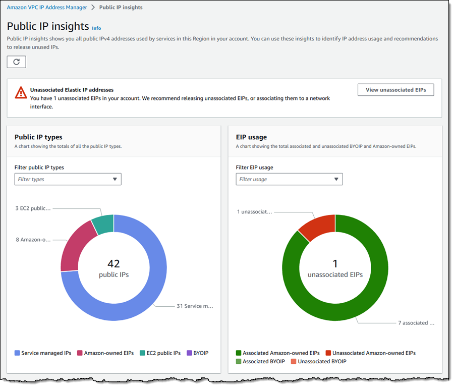
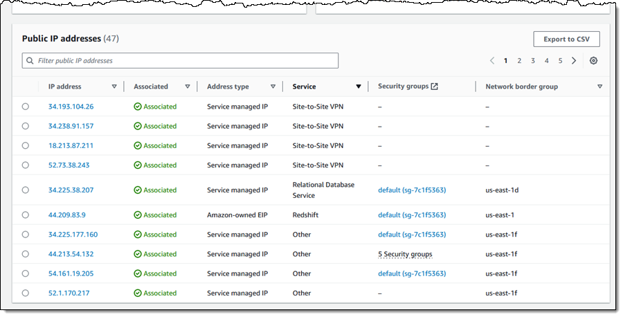
 Deepthi Mohan is a Principal Product Manager on the Amazon Kinesis Data Analytics team.
 Karthi Thyagarajan was a Principal Solutions Architect on the Amazon Kinesis team.


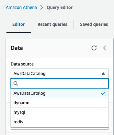
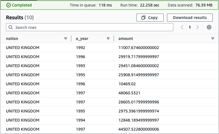
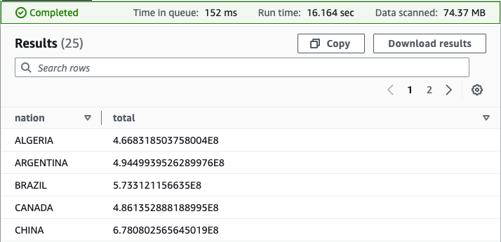
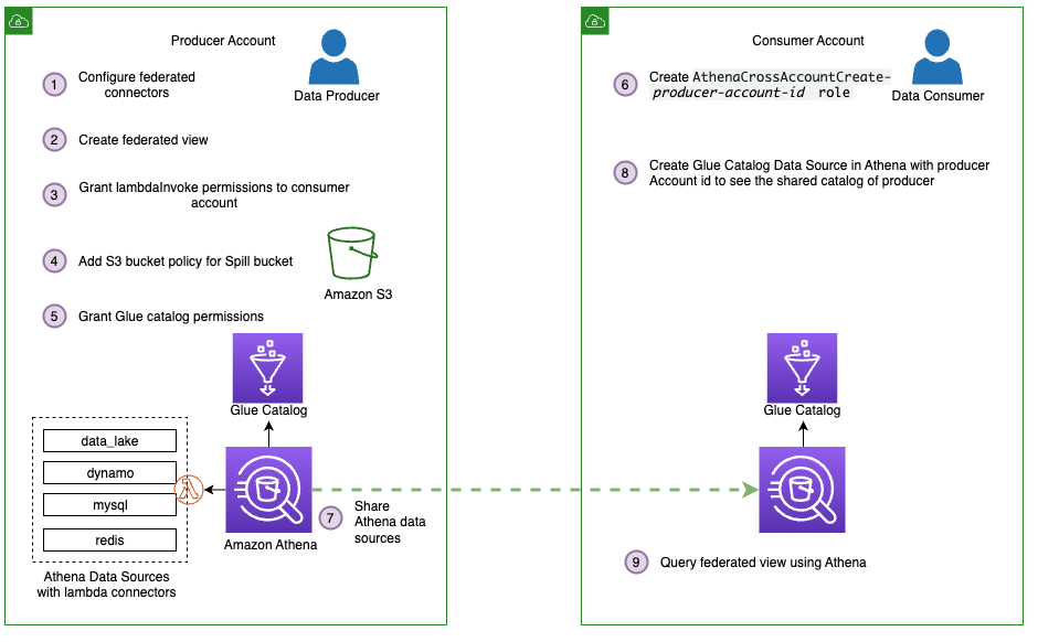
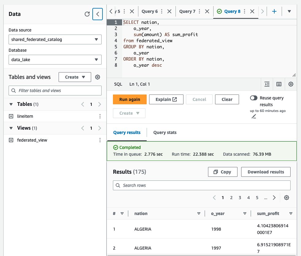

 Pathik Shah is a Sr. Big Data Architect on Amazon Athena. He joined AWS in 2015 and has been focusing in the big data analytics space since then, helping customers build scalable and robust solutions using AWS analytics services.




 Rohit Vashishtha is a Senior Analytics Specialist Solutions Architect at AWS based in Dallas, Texas. He has 17 years of experience architecting, building, leading, and maintaining big data platforms. Rohit helps customers modernize their analytic workloads using the breadth of AWS services and ensures that customers get the best price/performance with utmost security and data governance.



 Yadukishore Tatavarthi is a Senior Partner Solutions Architect supporting Healthcare and life science customers at Amazon Web Services. He has been helping the customers over the last 20 years in building the enterprise data strategies, advising customers on cloud implementations, migrations, reference architecture creation, data modeling best practices, data lake/warehouses architecture, and other technical processes.
 Sudhir Gupta is a Principal Partner Solutions Architect, Analytics Specialist at AWS with over 18 years of experience in Databases and Analytics. He helps AWS partners and customers design, implement, and migrate large-scale data & analytics (D&A) workloads. As a trusted advisor to partners, he enables partners globally on AWS D&A services, builds solutions/accelerators, and leads go-to-market initiatives
 Deepak Singh is a Senior Solutions Architect at Amazon Web Services with 20+ years of experience in Data & AIA. He enjoys working with AWS partners and customers on building scalable analytical solutions for their business outcomes. When not at work, he loves spending time with family or exploring new technologies in analytics and AI space.