As my home monitoring experiment has become such a celebrity and as it has so much going on, I’m trying to make sure I won’t ever lose its configuration and data, no matter what would happen. Here are some tips and reminders for you, too.
In the IT world, so much can go wrong. Hardware can die, files can become corrupt, malware can hit you, hackers can breach your systems, buggy software updates can cause havoc, you can fat-finger some commands or click on the wrong place and remove data… the list is endless. Here are some ways I’m attempting to protect my home monitoring environment.
Keep software updated
First things first. In today’s malicious world, it’s mandatory that you keep your software updated. With Linux and Zabbix, you don’t have an excuse to skip the updates. Updating your systems is fast and trouble-free. In small environments like home, even major Zabbix upgrades are fast as the database is not very big, so the database migrations that in a corporate environment can take time, will go through in minutes if not faster.
But I don’t trust one environment. What if my BackupPC says Kaboom? A nightly cron job also copies backup archives from my Raspberry Pi to my Mac, which in turn mirrors the backups to my iCloud. And, there’s one more cloud service I’m using for all my backups but not mentioning it here by name.
Test your backups
As long as you have not verified that your backups do actually work, you do not have a working backup. Have a virtual machine into which you can try to restore your backups. See if they work. Test them periodically, either manually or figure out an automated way to do that.
In the case of Zabbix, you can make your primary Zabbix monitor your test environment, and make Zabbix alert if your restore environment Zabbix suddenly starts responding back something else than the regular login page, or if the restore environment database doesn’t come back with some query response you would expect.
Setup a HA cluster
As any hardware can die, it’s not a bad idea to set up a HA cluster. Last winter I was preparing for potential electricity blackouts here in Finland and did setup my laptop to be a secondary node for my Zabbix. This setup has been working very well.
Use strong passwords
Even if it would only be your sandbox environment where you do test new stuff, please remember to use strong passwords. An evil actor can attempt to breach more targets in your network through a single point of failure.
Use ssh keys
Instead of username + password combination, use ssh keys for ssh authentication. Keys are immune to brute-force attempts and with tuning, ssh keys can also be allowed to only connect from specific IPs and run only specific commands. You know how in your ~/.ssh/authorized_keys the lines do start with something like
Obviously, this grants you much more security than traditional logins.
Use HashiCorp Vault
OK, I admit I’m not doing this at home as it would be overkill for my few logins. But, in a larger environment with absolutely critical safety requirements, use HashiCorp Vault for protecting your credentials. Zabbix has native support for it.
Monitor your logs
Setup a centralized log server — it can be your Zabbix server environment, too — and make sure you monitor the logs. My Zabbix gets all my logs, but wouldn’t be a bad idea to use more advanced log monitoring tools, too. Since I already do have ElastiFlow running at home, at some point I might start utilizing Elasticsearch for the logs. Not doing it much yet.
Use chkrootkit, AIDE, others
Tools like AIDE or chkrootkit can help you detect an intrusion. Set them to run in your cron and get alerted in case of any anomalies. Maybe I’ll one day integrate Zabbix with these tools.
Firewall your environment, use VPN
Don’t allow direct access from the Internet to your Zabbix, or your database, or anything really. In my case, my Asus router allows setting up OpenVPN connections, so that’s what I use. Whilst on the go, I just connect to OpenVPN on my phone and do whatever I need remotely through that.
Anything else?
Did I miss something? Let me know in the comments.
This post was originally published on the author’s page.
Abstract: We demonstrate how images and sounds can be used for indirect prompt and instruction injection in multi-modal LLMs. An attacker generates an adversarial perturbation corresponding to the prompt and blends it into an image or audio recording. When the user asks the (unmodified, benign) model about the perturbed image or audio, the perturbation steers the model to output the attacker-chosen text and/or make the subsequent dialog follow the attacker’s instruction. We illustrate this attack with several proof-of-concept examples targeting LLaVa and PandaGPT.
Ако наличието на бюджет, правителство и управленска програма са признаци за политическа нормалност, то значи България се нормализира. Летният политически сезон приключи с оптимизъм за бъдещето на ротацията между първите две политически сили – проводниците на нормалността. Първото съвместно изявление тази седмица на лидерите на управляващия съюз – Кирил Петков (ПП), Христо Иванов (ДБ) и Бойко Борисов (ГЕРБ), режисирано и напътствано от последния, даде заявка за общо бъдеще, по-силно от управленска програма.
Со кротце, со благо
Борисов посочи Иванов като „водач“ за съдебната реформа, когото ще следват, и „писмовния човек“, който ще подготви и предложи механизма за вземане на общите решения на двете коалиции. Макар този механизъм да беше обещан в пакет с управленската програма, така и не се появи. Пред bTV съпредседателят на ДБ Атанас Атанасов съобщи, че протокол за вземане на решения ще бъде подписан в началото на идната седмица. Всичко е уточнено, каза той. Но и без него управляващите се справят нелошо с вземането на решения – бързо се разбраха за ръководството на БНБ, опъват си нервите за НЗОК и Сметната палата, но не задълго. И за да прилича коалицията на истинска коалиция, демонстрират несъгласия по някои теми.
Най-прясно манифестираното негодувание беше свързано с бюджета и промените по проекта на финансовия министър Асен Василев, но на финала съществената част от тези промени – повишенията на заплати, бяха запазени, а отпаднаха и текстовете, срещу които протестираше ресторантьорският бранш. Данъкоплатците ще трябва да осигурят над 400 млн. лв. за повишени заплати, с които депутатите обремениха разходите, над една трета от които са за МВР.
Ревизиран беше първоначалният вариант фирми с 50 и повече души персонал да плащат заплатите само по банков път – запази се за тези със 100 и над 100 наети. В България техният брой е твърде малък. По данни на НСИ от края на 2022 г. в страната функционират общо 412 878 предприятия, от които 383 592, или почти 93%, имат персонал до 9 души, в 4436 работят между 50 и 249 наети, а с повече от 250 са едва 754, сред които телекомите, големите търговски вериги и др., собственост на големи международни компании.
Отпадна предложението на Министерството на финансите ресторантьорите да плащат възнагражденията само по банков път, независимо от броя на работещите. Браншът запази и ниската си ставка по ДДС от 9%, въведена заради пандемията от COVID-19. Асен Василев я защити, че помага за изсветляването на бизнеса, но не представи данни за „аргумента“ си. Парламентът отхвърли т.нар. безплатен обяд – идеята на Василев клиент на заведение да откаже да плати сметката, ако не получи касов бон.
Запазват се енергийните компенсации за бизнеса, здравните заведения, училища и храмове, подпомогнати за м.г. с над 6 млрд. лв. за купуваната от тях електроенергия от свободния пазар. ГЕРБ склониха и 350 млн. евро от оперативни програми, които ще останат неизразходвани, да се прехвърлят на Фонд „Сигурност на електроенергийната система“, а оттам – в Министерството на енергетиката, което ще ги внесе в бюджета.
Програма има, механизъм за решения – не
Наесен „не-коалицията“ ще е само ироничен прякор, „сглобката“ – забравен текст от SMS. Правителството публикува програма за управление, съгласувана с ПП–ДБ и ГЕРБ–СДС, и въпреки своите 146 страници документът не е особено амбициозен откъм реформи. Заявеното потвърждава известни от години цели, като еврозоната и Шенген, реализиране на Плана за възстановяване и устойчивост (ПВУ), овладяване на инфлацията и ефективно управление на общински проекти. За изпълнението до края на 2024 г. са вписани множество законопроекти, стратегии, концепции и наредби, част от които са свързани с наваксване заради срокове.
Датата за присъединяване към еврозоната е 1 януари 2025 г., а мащабна разяснителна кампания ще стартира през септември. Законът за въвеждане на еврото е предвиден като последен от необходимите за еврозоната – за април догодина. Според кабинета присъединяването към Шенгенското пространство предстои до края на 2023 г.
В програмата не са предвидени реформи за железниците, нито пък в здравеопазването, където българските граждани продължават да доплащат все повече и повече, но качеството на здравните услуги не се подобрява. Не се предлага и решение за острия недостиг на медицински сестри. И това правителство като други преди него е записало законови промени – със срок до ноември т.г., които да забранят създаване на нови болници „до утвърждаване на нова национална здравна карта“. (Лечебните заведения в България са 341, бюджетът на НЗОК, откъдето се финансират, е близо 7,03 млрд. лв. и по традиция лъвският пай – близо 47%, е предназначен за болниците.) Трудно е за вярване дали ще се случи, тъй като и предишните ограничения са издържали колкото и забраните за строителство по морето. За Националната детска болница обаче е предвидено до февруари 2024 г. да бъде готова техническата спецификация за обществена поръчка за проектирането на комплекса.
Освен предложение за изграждане на нови ядрени мощности в Козлодуй със срок декември 2024 г., други големи проекти не са разписани. Като най-амбициозни и детайлно разработени се отличават инициативите в енергетиката и образованието. Кабинетът „Денков–Габриел“ се надява да получи второто плащане по ПВУ през декември, година след първото. Декември е и заложеният срок, в който да представи в Европейската комисия преработения план, свързан с реформата в декарбонизацията на енергийния сектор.
До септември трябва да се проведат преговорите с Украйна за продажба на оборудването за АЕЦ „Белене“ – парламентът поиска да не е на цена, по-ниска от платената, т.е. под 660 млн. евро. Споменати са и ускорен ремонт и рехабилитация на ПАВЕЦ „Чаира“, за които се говори повече от година и половина, ефективно управление на енергийния преход на комплекса „Марица-изток“ – за което до момента политическа воля не се намери.
В управленската програма са записани и вече приключили действия, като приемането на бюджета за 2023 г., също и включването на държавата в търсене на нефт и природен газ в Черно море. Идеята е БЕХ да придобие дял от 20% в консорциума на Total и OMV, които търсят въглеводороди в „Блок 1-21 Хан Аспарух“.
До октомври ще бъдат пуснати търгове за изграждане на поне 285 MW капацитет за производство на евтина електроенергия от ВЕИ.
В сферата на образованието се обещава най-сетне да бъде готов, макар и през ноември 2024 г., стандартът за качество в училищното образование. Замислени са и други радикални промени, например въвеждане на тригодишно обучение за придобиване на бакалавърска степен. А до февруари правителството се е задължило да въведе национална система за проследяване на ранното детско развитие в яслите и в детските градини. Срокът за новите учебни програми обаче е учебната 2025/2026 г.
Съдебната реформа – сбъдната мечта?
Пред телевизионните камери тази седмица Бойко Борисов обеща мечтата на Христо Иванов за съдебна реформа, която не се е сбъднала преди десет години, да бъде сбъдната сега от „не-коалицията“. Преди десетилетие Иванов беше министър на правосъдието във второто правителство на Борисов, а сглобка на ГЕРБ, ДПС и БСП опраска конституционните промени. Сега е един от лидерите на коалиция, която ги предлага отново в комбинация с други, а Борисов е партньор в управлението.
Основните акценти в проекта за изменение на Конституцията са промяна на датата на националния празник – 24 май; не повече от два мандата на кметовете на общини; разделяне на ВСС на съдийски и прокурорски съвет, за да се осигури съдебната независимост; намаляване на мандата на главния прокурор и радикално ограничаване на правомощията му – идеята е да бъде само административен ръководител на Върховната касационна прокуратура; въвеждане на стандарт за избирането на регулаторните и контролните органи; трансформация на статута на служебните кабинети; възможност за подаване на индивидуална конституционна жалба от всеки гражданин.
ГЕРБ вече обяви, че не подкрепя ограничаването на кметските мандати и настоява за по-голям баланс в правомощията на служебните кабинети.
Засега проектът вдигна пушилка заради предложението, дошло от „Демократична България“ 24 май да стане националният празник на България, което означава, че ще замени 3 март. Целта според депутатката от ПП–ДБ Надежда Йорданова е „да вдигнем на конституционно ниво принципите, които изграждат българската държавност“. Някои предложения събудиха недоумението на конституционалисти и известни юристи като адвокат Михаил Екимджиев, който в интервю пред „Сега“ ги определи като националистическа доктрина, идентична с тази на Александър Дугин и Путин.
Чл. 3 от законопроекта гласи:
(1) Българската държавност се основава на ценностите на просвещението, духовността, свободата и равноправието, въплътени в идеите и делото на светите братя Кирил и Методий и техните ученици, на Апостола на българската свобода Васил Левски и на възрожденските будители и революционери. (2) В утвърждаване на тези ценности образованието, науката и културата и опазването на културно-историческото наследство са стратегически национални приоритети. (3) Официалният език в републиката е българският. Държавата гарантира и насърчава неговото опазване. (4) Всички исторически установени в България културни традиции са неразделна част от националното ни културно богатство.
Тези промени обаче тепърва ще се обсъждат, ще се оспорват в Конституционния съд и едва ли ще бъдат приети до края на годината, както беше съобщено. Конституционното мнозинство от ПП–ДБ, ГЕРБ–СДС и ДПС, което се е зарекло да внесе общ проект, едва ли ще бърза. Може и да чака ротацията на акад. Денков с кандидатката на ГЕРБ Мария Габриел в началото на март. В управленската програма конституционният проект е вписан без срок за изпълнение.
В раздел „Правосъдие“ на управленската програма обаче се откриват други интересни предложения, например Концепция за регулиране на лобистките дейности в Република България. Срокът да види бял свят е ноември, а се подготвя съвместно с Базелския институт за добро управление. До момента всички опити за регулиране на лобизма са удряли на камък, а законодателните идеи в тази посока са идвали все от ДПС.
По отношение на приетия на първо четене и застопорен законопроект за противодействие на корупцията, който предвижда реформа на структурата на КПКОНПИ и създаване на нова антикорупционна комисия с разследващи функции, управляващите чакат препоръки от Брюксел. Иначе проектът няма да стигне до обсъждане за второ гласуване в Комисията по правни въпроси.
Наесен коалицията трябва да започне подготовката на бюджета за 2024 г. и на обещаните законопроекти, а политическите сили – кампаниите си за местни избори. Всичко върви в коловозите на тройно гарантирана нормалност.
превод от румънски Лора Ненковска, София: изд. ICU, 2023
Гъста като петмез проза. Лепкав, сладостен, поетичен език, омаломощаващо внимание към детайла, което те повлича, сиропира читателския ти ум и като че ли парализира физическите реакции на ужаса, с който са изпъстрени тези страници. „Питай встрани“, казва моя позната терапевтка. „Пациентът следи с очи пръстите на аналитика, докато изважда травмата от дългосрочната памет и я депозира в краткосрочната“, гласи описанието на друг метод за справяне с посттравматичния синдром.
Кое дете е било, каза ли ти, а как изглеждаше, докато ти разказваше, спокоен ли беше, какъвто е обикновено, с тревожен поглед, с безразличен глас, който сякаш потъва в повея на вятъра…,
пита героинята по повод потрисаща история за канибализъм. И сякаш целият ѝ разказ, с всичките ѝ травми, потъва в тази извънредна сетивност: детството, полепнало във водна леща, миришещо на селски двор, на селски клозет, на топли тела, които се движат по средата на двора, докато детето гледа от тъмния прозорец; семейният живот, потънал в мътната вода в запушената мивка, изплувал като трупа на съпруга беглец през реката, която би трябвало да го отведе към Югославия, сиропиран като саварината, която съпругът изяжда преди това с любовницата си, а героинята отбелязва 1) начина, по който той най-напред маха маслената розичка от сладкиша, 2) пуловера, който самата тя му е купила и изпрала с шампоан, за да не губи мекотата си, 3) унижението да прочете за тази сцена в доноса на Секуритате…
Същата сцена виждаме и през погледа на сина, който години по-късно е отишъл да прочете досието на баща си – за да може, макар през омразния език на доносите, да събере частите от своята семейна история. Неговият език е като че по-прогледен, защото, докато майката се стреми да замъгли гледката на истината, синът се опитва да я открие. В този смисъл двамата вървят в противолопожни посоки – единият се опитва да се справи с травмите, като ги изтласка, другият – като си пробие път към тях, като разбере.
Някога ми каза, че ако хората вече ги няма, това не означава, че миналото им принадлежи на всички, всеки с неговата версия и интерпретация… Добре, бих ти отвърнал, но ако не можеш да научиш как точно са се случили нещата, това не значи, че не са се случили. Не можеш да ги изтриеш от историята само защото не ти е дадено да познаеш цялата истина за тях.
Третата част на книгата, озаглавена „Михалаки“, като че ли свидетелства за последния етап в преработването на истината – тогава, когато тя не е нито болезнено прясна, нито болезнено убеглива, а като че ли завинаги уталожена в ритмите на литературата. Отложена по-назад във времето, тя сякаш веднага придобива патината на мита. С други думи, историческият факт избелява и остава да изпъква главно образът – като този на слонския скелет в училищния кабинет по естествена история, където депутатите били заключени, докато не изберат нов княз. Но в същото време се наслагва и в историческата памет на самото място, и в преповтарящите се през поколения теми – като трудната и разпокъсана връзка между поколенията, като непрестанния мотив на сирачеството и отритнатостта.
Извънредно трудна като стилистика книга, бляскава преводаческа работа на Лора Ненковска.
превод от английски Ангел Игов, Пловдив: ИК „Жанет 45“, 2023
През юли 2008 г. жителите на Белград откриват, че в един от обикновените бетонни квартали е арестуван възрастен човек с вързана на опашка прошарена коса. Въпросният Драган е познат като духовен учител, проповядващ един вид православна мистика. Истинското му име обаче е Радован Караджич.
Повечето хора имат чувство за териториалност по отношение на истината.
Ние, българите, често смятаме, че трябва да знаем повече за Източна Европа от западния читател, не дай си боже от този, който е отдалечен от нас през океана. По тази причина статиите на Димитър Кенаров, писани за престижни американски списания, би трябвало леко да дразнят. Още повече – преводни. Още повече – написани умело, с литературен усет, пластичен език и космополитни препратки. Това ли момче ще ни каже кой живее в съседния вход?
Ами да. Защото
териториалната близост е илюзорна, ако не видиш нещо с очите си;
ако не отидеш с готовността да зададеш неудобен въпрос, да подхванеш нелицеприятна тема. Да бъдеш на места, различни от тези, на които ходят „хора като теб“. И аз съм била в Белград, но не би ми хрумнало да отида да видя как домът на Милошевич е превърнат в място за поклонение. Не съм била арестувана в Беларус. И реакцията ми в началото на войната в Украйна не е била да тръгна натам, за да видя с очите си какво става.
И все пак Димитър Кенаров не е типичният разследващ журналист; той не търси интервюта с главните герои от новинарските емисии. Вместо това отива на място и описва тяхната среда. Хората, които са ги направили възможни. Начина, по който реагираме след новината за чудовищното. Като отказваме да повярваме и се разпиляваме в конспиративни теории. Като опаковаме чудовищното като сензация, таблоиден гъдел, в който моралните съображения постепенно отпадат и запомняме само къде сме се хилили, надлежно погъделичкани по чакрите. Като в туристическата обиколка „Попарт Караджич“. Иначе казано,
най-важното в тези статии – това, което си струва човек да опише от първа ръка – е процесът на нормализация на ненормалното, преобразуването на нечовешкото в „човещинка“,
ключовата роля не на Хамлет или Клавдий, а на Розенкранц и Гилдернстерн. От Сърбия, от България, от Македония, от Полша, Беларус, поречието на Дунав, Ирак, Сараево, Украйна. И в тази роля е наистина важно да се видим отстрани. Или поне да осъзнаем, че сме видими.
Активните дарители на „Тоест“ получават постоянна отстъпка в размер на 20% от коричната цена на всички заглавия от каталозите на ICU и „Жанет 45“, както и на няколко други български издателства в рамките на партньорската програма Читателски клуб „Тоест“. За повече информация прочетете на toest.bg/club.
В емблематичната си колонка, започната още през 2008 г. във в-к „Култура“, Марин Бодаков ни представяше нови литературни заглавия и питаше с какво точно тези книги ни променят. Вярваме, че е важно тази рубрика да продължи. От човек до човек, с нова книга в ръка.
В първата част от поредицата, в която се опитваме да изясним феномена ранна бременност в България, разгледахме как се общува с децата в семейството и в училището по отношение на половото съзряване и какво е нивото на здравното образование у нас. В тази част ще разкажем какво се случва с една жена и нейното икономическо състояние, ако тя роди в тийнейджърска възраст.
Успява ли да стъпи на трудовия пазар, ако изобщо никога не е работила, тъй като ражда на 16 години? Намира ли си работа, която ѝ позволява да е финансово независима и да е квалифицирана и високоплатена? Как може да се мотивира човек в подобна ситуация да стане активна част от обществото и да не изпитва срам, че е по-възрастен от съучениците или колегите си? Как влияе ранната бременност на икономическите възможности на бъдещите поколения?
Тука има, тука няма данни
Колко от майките в България, които раждат рано, успяват да завършат образованието си? Или кога започват първата си работа? Не знаем. Докато за други държави, като САЩ, има изключително подробна статистика колко завършват или работят след бременност в тийнейджърска възраст, у нас данни липсват. В САЩ едва 50% от майките, родили в тийнейджърска възраст, завършват гимназия до 22 години, в сравнение с 90% от жените, които не раждат, преди да излязат от пубертета. Едва 10% от жените, минали през ранна бременност в САЩ, завършват 2- или 4-годишна програма за висше образование.
В България данните за раждаемостта по възраст се генерират от Националния статистически институт (НСИ), като проблемът е обобщеният вид, в който се представя информацията. Имаме данни за броя жени, родили под 20-годишна възраст, но не и как тенденцията се изменя през годините. Липсва публична информация за раждаемостта в категориите 10–14 и 15–19 години, като за тези възрастови групи са налице единствено данни за общата плодовитост. НСИ тълкува плодовитостта като „среден брой деца, които би родила една жена през целия си фертилен период съобразно повъзрастовата плодовитост през отчетната година“, но това не дава яснота колко момичета са станали майки в конкретен период.
Никаква по-детайлна статистика за социално-икономическата обремененост на една жена, която е родила рано, не е налице. Подобна информация би дала представа за домакинството, в което жената е отраснала, включително за историята на ранна бременност в семейството, посещението на училище през детството (преди забременяването), развитието ѝ, след като роди, и др.
Макар да говорим за това как една жена става част от трудовия пазар след ранна бременност, образованието има своето място и в тази история – то е ключов фактор в уравнението на ранното забременяване. Радосвета Стаменкова, изпълнителната директорка на Българската асоциация по семейно планиране и сексуално здраве (БАСП), е убедена в това. Според Стаменкова, за да не забременяват момичета в ранна възраст, е много важно да се работи за предотвратяване на ранното им отпадане от училище. Битката за оставането им в класните стаи е битка за бъдещето им, защото със завършването на средното им образование възможността за реализация, различна от това да станат майки на 16 години и да останат майки през целия си живот, се увеличава.
По данни на НСИ за 2022 г. само половината (!) от завършилите основно образование в България успяват да завършат и средното си образование. Ако през 2018 г. малко над 71 000 ученици получават основно образование, то през 2022 г. едва 36 000 вземат диплома за средно. Тук е важно да се отбележи, че през 2018 г. влизат в сила промените, според които основно образование се завършва в седми, а не в осми клас, и така цялостната статистика за конкретния випуск се размества. Освен това няколко хиляди ученици продължават гимназиалното си образование в чужбина поради емиграция на семейството или просто като образователен избор. Те също влизат в тази статистика на „отпадналите“. Какво се случва с останалите? Къде са?
Ето в тази статистика са и онези момичета, които стават майки рано и впоследствие изпитват затруднения да завършат образованието си поради новопоявилите се задължения покрай детето или да се квалифицират, за да си намерят работа. Само че нямаме точни данни тъкмо за това.
Отново по данни на НСИ от 2022 г. нивото на образование оказва съществено влияние върху риска от бедност. Най-високият дял на работещи бедни е налице при хората без образование или само с начално – 68,5%. Разликата между основното и средното образование е осезаема – 32,9% от хората с основно образование са работещи бедни, докато при завършилите ХII клас процентът е 8,8%.
Разбирането на връзката между ранната бременност и трудовата заетост е сложно поради многото променливи величини, които влияят на възможностите на една жена да стане част от трудовия пазар. Ясно е, че у нас няма такива данни, за да можем да съпоставим по научно изпитан начин две средностатистически жени и да разгледаме кои са факторите, поради които едната е родила рано, а другата – не. Затова цялата дискусия по оста ранно забременяване – трудова заетост не е толкова прецизна, колкото би ни се искало.
При всички положения е сигурно, че образованието е първата стъпка към по-голям шанс за квалифицирана и достойно платена работа, защото то екипира жената с уменията да взема решения и да се развива. В българското общество остава прието основната част от грижите за едно дете, а следователно и компромисите с личния живот да се поемат от майката. Напускането на училище след забременяване не е изненадващо, като най-важният фактор е грижата, която момичето трябва да положи за детето си, но са налице и други, като стигматизирането от връстниците и семейството.
Всеки случай е отделен, но повечето научни изследвания говорят, че жените, които раждат първото си дете в юношеска възраст и не завършват образованието си, обикновено имат деца и внуци, за които е по-малко вероятно да завършат образованието си. Иначе казано, ранната бременност има преки ефекти върху бъдещите доходи и икономическото състояние на няколко поколения в едно домакинство. Унаследеността на проблема създава социално-икономически цикъл, в който се въртят хора с ограничени възможности, ограничени умения и ограничен достъп до пазара на труда.
Културата на отчаяние
Ранното забременяване на една жена не е резултат от факта, че тя е от конкретен етнос, както често се смята у нас, а че е част от маргинализирана общност и среда с ниски доходи. Юношеската бременност обикновено не е резултат от съзнателен избор, а по-скоро произтича от липсата му, когато става въпрос за брак и употреба на контрацептиви.
„Културата на отчаяние“ е понятие, с което се назовава причинно-следствената връзка между социално-икономическата среда, в която расте едно момиче, и шанса то да забременее в юношеските си години. Понятието е развито от изследователите Мелиса Кърни и Филип Ливайн, работещи съответно към Центъра за изследване на населението в Университета на Мериленд и „Уелсли Колидж“. Двамата се позовават на данни, обхващащи над 42 000 жени в периода 1982–2008 г. в САЩ, и използват набор от похвати на иконометричното моделиране, за да отчетат и допълнителните фактори, влияещи върху раждаемостта сред тийнейджърките, като раса, етнос, религия и др.
Работата на изследователите е базирана на по-ранни социологически проучвания, в които се разглежда формирането на специфични места с константна бедност, дължаща се на липса на възможности, социална изолация и отлъчване от пазара на труда. Кърни и Ливайн твърдят, че комбинацията от бедност и живот в социално неравенство, водеща до засиленото чувство за липса на перспективи, е ключовият фактор за тийнейджърската бременност.
В България по последни данни на НСИ за 2022 г. относителният дял на бедните спрямо линията на бедността е 22,9% общо за страната. Към датата на публикуване на изследването линията на бедност в България е 413 лв., а към днешна дата е 504 лв. В контекста на тези данни е важно да се споменат поне още два фактора, които биха могли да са част от пътя, водещ до бременност в юношеска възраст. Първо, жените са в по-голям риск от бедност, тъй като 25,8% от тях в сравнение с 19,9% от мъжете са в горната статистика. Тази тенденция е растяща – през 2018 г. процентът за жените е бил 23,4. Шансът за една жена да излезе от тази статистика не е особено голям, ако съдим по измерванията на социалната мобилност.
По данни на Световната банка неравенството в доходите в България се увеличава през последните десетилетия. Казано по-просто, пропастта между богати и бедни расте и е все по-трудно да повишиш доходите си, ако тръгваш от ниско финансово стъпало. Тоест дори по-голямата част от ражданията на възраст под 18 години, които сме свикнали да виждаме отразявани по медиите, да се свързват с ромските общности, това не е етнически феномен, а феномен на бедността. Радосвета Стаменкова разказва, че има и момичета от български произход, които поради неинформираност, незнание, неизползване на контрацептиви стигат до забременяване в ранна възраст. Те просто нямат стигма върху върху себе си, прекратяват бременността и не влизат в статистиката.
Политики на килограм
А как изобщо се правят политики, ако няма данни, на които да се основават? Не можем като общество сериозно да оценим доколко ранното забременяване влияе на икономиката ни и на бъдещите поколения, ако гледаме на него само като присъщо на ромската общност.
Политиките на едро могат да са ефективни, но не и когато става въпрос за неравенство и изваждане на хората от цикъла на бедността. В това е сигурен Адриан Николов, икономист в Института за пазарна икономика, с фокус върху пазара на труда, бедността и неравенството у нас, с когото „Тоест“ говори по темата. Когато става въпрос как се отнасяме към елиминиране на неравенствата, Адриан смята, че инструментите на държавата не са подредени правилно.
В момента се занимаваме с това да осигуряваме временна заетост на безработните, да повишаваме доходите на всички поравно, да се фокусираме върху програми, които засягат цялото население.
За пример той дава решението на парламента от по-рано тази година, с което се прие всички ученици да получават безплатни учебници от учебната 2024/2025 г. нататък. Изчисленията досега показват, че тази мярка ще струва на бюджета около 80 млн. лв.
Нека бъде ясно: това най-вероятно ще помогне на учениците в затруднено положение да останат в училище. Според изследване на Фондация „Тръст за социална алтернатива“ 6% от българските ученици отпадат от образователната система поради крайна бедност. В изследването се твърди, че безплатните учебници и транспортните възможности са ключови за по-голям достъп до образованието. Но…
От гледна точка на неравенството, когато дадем на цялата доходна структура по 100 лв., ние сме неутрални към него, защото резултатът остава същият. Ако дадем само на бедните по 500 лв., тогава техният доход ще се повиши спрямо богатите. Ако се опитаме наистина да свиваме разликата между бедните и богатите, то доходни тестове, таргетиране на хора в нужда, които са наистина бедни, и други подобни мерки биха били адекватни.
Адриан Николов също обръща внимание на липсата на данни, когато става въпрос за подкрепа на майките в крайна нужда. Макар да знаем, че средната възраст при първо раждане в София е 30,7 години, а в Сливен – 23,8 години, според него няма систематични анализи за нуждите на домакинствата и регионите, върху които трябва да се фокусираме.
Ние даваме майчинство поравно, независимо как функционира домакинството. Почти всички помощи, които са свързани с отглеждане на деца и майчинство, по никакъв начин не са обвързани с конкретна необходимост.
И макар този тип финансови субсидии, заместващи дохода, далеч да не са единственото, от което се нуждае едно семейство, те са най-доброто, предлагано от държавата ни за момента, и промяната им в период на демографски срив съвсем не е решението, както предупреждава Адриан Николов. Но според него индивидуалният подход към потребностите на всеки отделен случай е успешен модел за справяне с неравенствата, бедността и социалното изключване на хора и групи от хора. „Въпросът е как да прилагаме политики, които са насочени към конкретните потребности на конкретното домакинство и човек. Защото когато се опитваме да решаваме проблемите на всички, най-вероятно не помагаме на никого“, завършва Николов.
Той е съгласен, че липсата на образование до голяма степен възпрепятства една жена да е активна на пазара на труда и следователно да има шанс да излезе от кръга на бедност.
У нас средното образование е големият решаващ фактор, който на практика гарантира заетост, води до много голямо повишаване на заплатата в сравнение с хората с по-ниско образование.
Но отвъд превенцията, т.е. развитието на социални „обезопасителни мрежи“, които да задържат момичетата в училище, има какво да се направи и за етапа, в който те си търсят работа. Ключовата дума тук е „гъвкавост“ или „заетост на непълен работен ден“. „Майките успяват да съчетават грижата за децата и работата чрез подобни възможности за заетост. Те създават голям мост между бременността, отглеждането на дете и пазара на труда“, допълва Адриан Николов.
В заключение, смисленото подпомагане на която и да е група – било то млади майки, работещи бедни или комбинацията от двете – изисква набор от мерки и промени от страна на държавата и обществото. Такива са намаляване на социалното неравенство в страната, подобряване на достъпа до образование, развиване на националната статистика в детайли и еволюция на трудовия пазар към модел, който подкрепя, а не дискриминира жените, грижещи се за дете, без значение на каква възраст са родили. Всички тези мерки влизат под шапката на икономическото приобщаване и развитието на средата, в която растат младите момичета.
Може и да няма категоричен отговор на въпроса дали бедността винаги предшества ранната бременност, или е цикъл, подобен на казуса с яйцето и кокошката. Но това не е пречка да видим, че проблемите на младите майки у нас са пресечна точка на редица нерешени социално-икономически задачи. Въпросът е имаме ли намерение да се заемем с тези задачи, или винаги ще има нещо по-важно, докато накрая не стане прекалено късно за каквото и да е решение.
любовта е мрежа. Любовта е ръце, които мятат мрежата. Любовта е кораб, който пренася рибата. Любовта е готвач, който я пържи. Любовта е уста, която я сдъвква, хранопровод, който я прекарва, стомах и черва, които я смилат, пръст, която поема рибешкия скелет, перките, люспите, червата, недоядените остатъци.
Преди теб бях риба, която плува в студеното море заедно с други риби, безразлична и свободна. Сега съм пържен скелет, готов да се разложи, да натори земята със себе си и да гледа небето, което от морето не се виждаше никога.
Албена Тодорова
Албена Тодорова (р. 1983) е авторка на три стихосбирки. Финансист по професия. След десет години в Япония, Германия и Великобритания, в момента живее в София. Стихотворението на месеца е част от книгата ѝ „Ще ти бъда тяло“, която се очаква да излезе през 2023 г. в ИК „Жанет 45“.
Според Екатерина Йосифова „четящият стихотворение сутрин… добре понася другите часове“ от деня. Убедени, че поезията държи умовете ни будни, а сърцата – отворени, в края на всеки месец ви предлагаме по едно стихотворение. Защото и в най-смутни времена доброто стихотворение е добра новина.
We launched Amazon EC2 C7g instances in May 2022 and M7g and R7g instances in February 2023. Powered by the latest AWS Graviton3 processors, the new instances deliver up to 25 percent higher performance, up to two times higher floating-point performance, and up to 2 times faster cryptographic workload performance compared to AWS Graviton2 processors.
Graviton3 processors deliver up to 3 times better performance compared to AWS Graviton2 processors for machine learning (ML) workloads, including support for bfloat16. They also support DDR5 memory that provides 50 percent more memory bandwidth compared to DDR4. Graviton3 also uses up to 60 percent less energy for the same performance as comparable EC2 instances, which helps you reduce your carbon footprint.
The C7g instances are well suited for compute-intensive workloads, such as high performance computing (HPC), batch processing, ad serving, video encoding, gaming, scientific modeling, distributed analytics, and CPU-based machine learning inference. The M7g instances are for general purpose workloads such as application servers, microservices, gaming servers, mid-sized data stores, and caching fleets. The R7g instances are a great fit for memory-intensive workloads such as open-source databases, in-memory caches, and real-time big data analytics.
Today, we’re adding a d variant to all three instance families. The new Amazon EC2 C7gd, M7gd, and R7gd instance types have NVM Express (NVMe) locally attached up to 2 x 1.9 TB SSD drives that are physically connected to the host server and provide block-level storage that is coupled to the lifetime of the instance. These instances have up to 45 percent better real-time NVMe storage performance than comparable Graviton2-based instances.
These are a great fit for applications that need access to high-speed, low-latency local storage, including those that need temporary storage of data for scratch space, temporary files, and caches. The data on an instance store volume persists only during the life of the associated EC2 instance.
Here are the specs for these instances:
Instance Size
vCPU
Memory (GiB)
Local NVMe Storage (GB)
Network Bandwidth (Gbps)
EBS Bandwidth (Gbps)
C7gd/M7gd/R7gd
C7gd/M7gd/R7gd
C7gd/M7gd/R7gd
medium
1
2/ 4 / 8
1 x 59
Up to 12.5
Up to 10
large
2
4 / 8 / 16
1 x 118
Up to 12.5
Up to 10
xlarge
4
8 / 16 / 32
1 x 237
Up to 12.5
Up to 10
2xlarge
8
16 / 32 / 64
1 x 474
Up to 15
Up to 10
4xlarge
16
32 / 64 / 128
1 x 950
Up to 15
Up to 10
8xlarge
32
64 / 128 / 256
1 x 1900
15
10
12xlarge
48
96 / 192/ 384
2 x 1425
22.5
15
16xlarge
64
128 / 256 / 512
2 x 1900
30
20
These instances are built on the AWS Nitro System, a combination of AWS-designed dedicated hardware and a lightweight hypervisor that allows the delivery of isolated multitenancy, private networking, and fast local storage. They provide up to 20 Gbps Amazon Elastic Block Store (Amazon EBS) bandwidth and up to 30 Gbps network bandwidth. The 16xlarge instances also support Elastic Fabric Adapter (EFA) for applications that need a high level of inter-node communication.
Now Available Amazon EC2 C7gd, M7gd, and R7gd instances are now available in the following AWS Regions: US East (Ohio), US East (N. Virginia), US West (Oregon), and Europe (Ireland). As usual with Amazon EC2, you only pay for what you use. For more information, see the Amazon EC2 pricing page.
If you’re optimizing applications for Arm architecture, be sure to have a look at our Getting Started collection of resources or learn more about AWS Graviton3-based EC2 instances.
I am happy to announce that a new AWS Local Zone in Phoenix, Arizona is now open and ready for you to use, with more instance types, storage classes, and services than ever before.
We launched the first AWS Local Zone in 2019 (AWS Now Available from a Local Zone in Los Angeles) with the goal of making a select set of EC2 instance types, EBS volume types, and other AWS services available with single-digit millisecond when accessed from Los Angeles and other locations in Southern California. Since then, we have launched a second Local Zone in Los Angeles, along with 15 more in other parts of the United States and another 17 around the world, 34 in all. We are also planning to build 19 more Local Zones outside of the US (see the Local Zones Locations page for a complete list).
Local Zones In Action Our customers make use of Local Zones in many different ways. Popular use cases include real-time gaming, hybrid migrations, content creation for media & entertainment, live video streaming, engineering simulations, and AR/VR at the edge. Here are a couple of great examples that will give you a taste of what is possible:
Arizona State University (ASU) – Known for its innovation and research, ASU is among the largest universities in the U.S. with 173,000 students and 20,000 faculty and staff. Local Zones help them to accelerate the delivery of online services and storage, giving them a level of performance that is helping them to transform the educational experience for students and staff.
DISH Wireless -Two years ago they began to build a cloud-native, fully virtualized 5G network on AWS, making use of Local Zones to support latency-sensitive real-time 5G applications and workloads at the network edge (read Telco Meets AWS Cloud to learn more). The new Local Zone in Phoenix will allow them to further enhance the strength and reliability of their network by extending their 5G core to the edge.
We work closely with these and many other customers to make sure that the Local Zone(s) that they use are a great fit for their use cases. In addition to the already-strong set of instance types, storage classes, and services that are part-and-parcel of every Local Zone, we add others on an as-needed basis.
And Now, Phoenix As I mentioned earlier, this Local Zone has more instance types, storage classes, and services than earlier Local Zones. Here’s what’s inside:
Instance Types – Compared to all other Local Zones with the T3, C5(d), R5(d), and G4dn instance types, the Phoenix Local Zone includes C6i, M6i, R6i, and Cg6n instances.
EBS Volume Types – In addition to the gp2 volumes that are available in all Local Zones, the Phoenix Local Zone includes gp3 (General Purpose SSD) , io1 (Provisioned IOPS SSD) , st1 (Throughput Optimized HDD), and sc1 (Cold HDD) storage.
Pricing Models – In addition to On-Demand and Savings Plans, the Phoenix Local Zone includes Spot.
Going forward, we plan to launch more Local Zones that are similarly equipped.
Opting-In to the Phoenix Local Zone The original Phoenix Local Zone was launched in 2022 and remains available to customers who have already enabled it. The Zone that we are announcing today can be enabled by new and existing customers.
To get started with this or any other Local Zone, I must first enable it. To do this, I open the EC2 Console, select the parent region (US West (Oregon)) from the menu, and then click EC2 Dashboard in the left-side navigation:
Then I click on Zones in the Account attributes box:
Next, I scroll down to the new Phoenix Local Zone (us-west-2-phx-2), and click Manage:
I click Enabled, and then Update zone group:
I confirm that I want to enable the Zone Group, and click Ok:
And I am all set. I can create EBS volumes, launch EC2 instances, and make use of the other services in this Local Zone.
At Rapid7 we love a good pen test story. So often they show the cleverness, skill, resilience, and dedication to our customer’s security that can only come from actively trying to break it! In this series, we’re going to share some of our favorite tales from the pen test desk and hopefully highlight some ways you can improve your own organization’s security.
Rapid7 was engaged to do an AWS cloud ecosystem pentest for a large insurance group. The test included looking at internal and external assets, the AWS cloud platform itself, and a configuration scan of their AWS infrastructure to uncover gaps based on NIST’s best practices guide.
I evaluated their external assets but most of the IPs were configured to block unauthorized access. I continued to test but did not gain access to any of the external assets since, with cloud, once access has been blocked from the platform itself there is not a lot that I could do about it. But nevertheless, I continued to probe for cloud resources, namely S3 buckets, AWS Apps etc., using company-based keywords. For example: companyx, companyx.IT, companyx.media, etc. Eventually, I found S3 buckets that were publicly available on their external network. These buckets contained sensitive information which definitely was a point of action for the client.
My next step was to complete a configuration scan of their AWS network, which provided complete visibility into their cloud infrastructure, including the resources that were running, the roles attached to the resources, the open services, etc. It also provided the customer valuable insights on the security controls that were missing based on the NIST’s best practices guide like the list of unused access keys, unencrypted disk volumes, keys that are not rotated every 90 days, insufficient logging, publicly accessible services like SSH, RDP, and many more. This scan was done using Rapid7’s very own InsightCloudSec tool which provides customers visibility into their cloud network and helps them identify gaps.
When testing the AWS cloud platform with the read-only credentials provided by the customer, I found they were locked with a strong IAM policy which allowed viewing of only cloud resources on the platform. However, there were no weaknesses in the IAM policy after attempts to enumerate vulnerabilities. This will be important later on!
Hardcoded credentials were found in Functions Apps and EC2 instance data but I was unable to utilize this further to escalate privileges. After enumerating the S3 buckets using the read-only credentials multiple S3 buckets containing customer invoices and payment data, along with Infrastructure-as-a-code files were found. This provided information about how the customer managed their automated deployments. Beyond this, we were unable to find any vulnerabilities to escalate privileges, however, all the data accumulated during the phase was kept handy in case there would be a chance to chain vulnerabilities together and gain access during the next phases of the pentest. Although it was frustrating to not be able to find any ways to escalate privileges from the platform itself, enumerating it gave me plenty of understanding about their environment which would prove useful in the next phase.
In the final phase of the test, I tested all of the internal assets that were in-scope. These were primarily windows servers on EC2 instances hosting different kinds of services and applications. I enumerated the Active Directory Domain controllers on these servers and found that some AD servers allowed for NULL session enumeration which means you could connect to the AD server and dump out all of the domain information like users, groups, and password policies, without authentication.
Password spray attacks were deployed after all the users from the Domain were accessed. Pretty quickly, it was clear there were multiple users using weak passwords like Summer2023, Winter23, or Password1. Many accounts were even sharing the same passwords! This provided plenty of compromised credentials allowing me to go through the access levels provided to these compromised accounts. I found one account with Domain Admin access and dumped the NTDS.dit file from the AD Servers which contained hashes for all the domain users. With this, several accounts with weak passwords were cracked.
With access to multiple accounts in the bag, the only goal left was to gain some sort of access on the AWS platform. With all the data gathered from the AWS cloud platform test, I first looked at the EC2 Instances on the platform and what roles were assigned to each of them. Then I assessed accounts which had admin access. I found an ‘xx-main-ec2-prod’ role attached to an EC2 instance for which I had admin access through one of the compromised accounts. Using RDP to login to the EC2 instance, I pinged the IAM meta-data server and got the temporary AWS credentials for the ‘xx-main-ec2-prod’ role.
With these credentials, I created a new AWS profile and enumerated the permissions associated with this role. The ‘xx-main-ec2-prod’ role had access to list secrets in the AWS account, put and delete objects on all S3 buckets, send OS commands to all EC2 instances in the AWS account, and modify logs, as well. I proceeded to list some secrets in the AWS account to confirm the access that we had gained. With this level of access, I was able to show the client how an attacker could escalate privileges on their AWS platform.
In the end, this testing highlights how vast the attack surface would be on the cloud network. Even if you’ve locked down your cloud platform, the infrastructure assets could be vulnerable allowing attackers to compromise them and then laterally move to the cloud network. As organizations move their networks to the cloud, it would be important for them not to simply depend on the cloud platform to secure their network but also ensure that their individual assets are continuously tested and secured.
Check us out at this year’s Black Hat USA in Las Vegas! Our experts will be giving talks and our booth will be staffed with many members of our team. Stop by and say hi.
This post is written by Ramesh Mathikumar, Senior DevOps Consultant and Francesco Vergona, Solutions Architect.
AWS Lambda now supports Python 3.11 as both a managed runtime and container base image. Python 3.11 contains significant performance enhancements over Python 3.10. Features like reduced startup time, streamlined stack frames and CPython specialization adaptive interpreter help many workloads using Python 3.11 run faster and cheaper, thanks to Lambda’s per-millisecond billing model. With this release, Python developers can now take advantage of new features and improvements introduced in Python 3.11 when creating serverless applications on Lambda.
You can use Python 3.11 with Lambda Powertools for Python, a developer toolkit to implement Serverless best practices and increase developer velocity. Lambda Powertools includes proven libraries to support common patterns such as observability, parameter store integration, idempotency, batch processing, feature flags, and more. Learn more about PowerTools for AWS Lambda for Python in the documentation.
You can also use Python 3.11 with Lambda@Edge, allowing you to customize low-latency content delivered through Amazon CloudFront.
Python is a popular language for building serverless applications. The Python 3.11 release includes both performance improvements and new language features. For customers who deploy their Lambda functions using container image, the base image for Python 3.11 also includes changes to make managing installed packages easier.
This blog post reviews these changes in turn, followed by an overview of how you can get started with Python 3.11 in Lambda.
Performance improvements
Optimizations to CPython introduced by Python 3.11 brings significant performance enhancements, making it an average of 25% faster than Python 3.10, based on Python community benchmark tests using the Python Performance Benchmark Suite.
This release focuses on two key areas:
Faster startup: core modules essential for Python are now “frozen,” with statically allocated code objects, resulting in a 10–15% faster interpreter start up relative to Python 3.10.
Faster function execution: improvements include streamlined frame creation, in-lined Python function calls for reduced C stack usage, and the implementation of a Specializing Adaptive Interpreter, which specializes the interpreter for “hot code” (code that’s executed multiple times) and reducing the overhead during execution.
These optimizations can improve performance by 10-60% depending on the workload. In the context of a Lambda function execution, this results in performance improvements for both ”cold start“ and ”warm start“ invocations
In addition to faster CPython performance improvements, Python 3.11 also provides performance improvements across other areas. For example:
String formatting with printf-style% codes is now as fast as f-string expressions.
Integer division is around 20% faster on x86-64 for certain scenarios.
Operations like sum() and list resizing have seen notable speed enhancements.
Dictionaries save memory by not storing hash values when keys are Unicode objects.
Improvements to asyncio. DatagramProtocol introduce significantly faster large file transfers over UDP.
Math functions, statistics functions, and unicodedata.normalize() also benefit from substantial speed improvements.
Language features
Thanks to its simplicity, readability, and extensive community support, Python is a popular language for building serverless applications. The Python 3.11 release includes several new language features, including:
Variadic generics (PEP 646): Python 3.11 introduces TypeVarTuple, enabling parameterization with an arbitrary number of types.
Marking individual TypedDict items as required or not-required (PEP 655): The introduction of Required and NotRequired in TypedDict allows for explicit marking of individual item requirements, eliminating the need for inheritance.
Self type (PEP 673): The Self annotation simplifies the annotation of methods returning an instance of their class, similarly to TypeVar in PEP 484
Arbitrary literal string type (PEP 675): The LiteralString annotation allows a function parameter to accept any literal string type, including strings created from literals.
Data class transforms (PEP 681): The @dataclass_transform() decorator enables objects to utilize runtime transformations for dataclass-like functionalities.
Change in pre-installed modules location and search path
Previously, Lambda base container images for Python included the /var/runtime directory before the /var/lang/lib/python3.x directory in the search path. This meant that packages in /var/runtime are loaded in preference to packages installed via pip into /var/lang/lib/python3.x. Since the AWS SDK for Python (boto3/botocore) was pre-installed into /var/runtime, this made it harder for base container images customers to upgrade the SDK version.
With the Python 3.11 runtime, the AWS SDK and its dependencies are now pre-installed into the /var/lang/lib/python3.11 directory, and the search path has been modified so this directory has precedence over /var/runtime. This change means customers who build and deploy Lambda functions using the Python 3.11 base container image can now override the SDK simply by running pip install on a newer version. This change also enables pip to verify and track that the pre-installed SDK and its dependencies are compatible with any customer-installed packages.
This is the default sys.path before Python 3.11 (where X.Y is the Python major.minor version):
/var/task/: User Function
/opt/python/lib/pythonX.Y/site-packages/: User Layer
Here is the default sys.path starting from Python 3.11:
/var/task/: User Function
/opt/python/lib/pythonX.Y/site-packages/: User Layer
/opt/python/: User Layer
/var/lang/lib/pythonX.Y/site-packages/: Pre-installed modules and default pip install location
/var/runtime/: No pre-installed modules
Using Python 3.11 in Lambda
AWS Management Console
To use the Python 3.11 runtime to develop your Lambda functions, specify a runtime parameter value Python 3.11 when creating or updating a function. Python 3.11 version is now available in the Runtime dropdown in the Create function page.
To update an existing Lambda function to Python 3.11, navigate to the function in the Lambda console, then choose Edit in the Runtime settings panel. The new version of Python is available in the Runtime dropdown:
AWS Lambda – Container Image
Change the Python base image version by modifying FROM statement in the Dockerfile:
FROM public.ecr.aws/lambda/python:3.11
# Copy function code
COPY lambda_handler.py ${LAMBDA_TASK_ROOT}
In AWS SAM, set the Runtime attribute to python3.11 to use this version.
AWSTemplateFormatVersion: '2010-09-09'
Transform: AWS::Serverless-2016-10-31
Description: Simple Lambda Function
  MyFunction:
    Type: AWS::Serverless::Function
    Properties:
      Description: My Python Lambda Function
      CodeUri: my_function/
      Handler: lambda_function.lambda_handler
      Runtime: python3.11
AWS SAM supports generating this template with Python 3.11 out of the box for new serverless applications using the sam init command. Refer to the AWS SAM documentation here.
AWS Cloud Development Kit (AWS CDK)
In the AWS CDK, set the runtime attribute to Runtime.PYTHON_3_11 to use this version. In Python:
from constructs import Construct
from aws_cdk import ( App, Stack, aws_lambda as _lambda )

class SampleLambdaStack(Stack):
    def __init__(self, scope: Construct, id: str, **kwargs) -> None:
        super().__init__(scope, id, **kwargs)

        base_lambda = _lambda.Function(self, 'SampleLambda',
                                       handler='lambda_handler.handler',
                                    runtime=_lambda.Runtime.PYTHON_3_11,
                                 code=_lambda.Code.from_asset('lambda'))
In TypeScript:
import * as cdk from 'aws-cdk-lib';
import * as lambda from 'aws-cdk-lib/aws-lambda'
import * as path from 'path';
import { Construct } from 'constructs';

export class CdkStack extends cdk.Stack {
  constructor(scope: Construct, id: string, props?: cdk.StackProps) {
    super(scope, id, props);

    // The code that defines your stack goes here

    // The python3.11 enabled Lambda Function
    const lambdaFunction = new lambda.Function(this, 'python311LambdaFunction', {
      runtime: lambda.Runtime.PYTHON_3_11,
      memorySize: 512,
      code: lambda.Code.fromAsset(path.join(__dirname, '/../lambda')),
      handler: 'lambda_handler.handler'
    })
  }
}
We are excited to bring Python 3.11 runtime support to Lambda and empower developers to build more efficient, powerful, and scalable serverless applications. Try Python 3.11 runtime in Lambda today and experience the benefits of this updated language version and take advantage of improved performance and new language features. For more serverless learning resources, visit Serverless Land
The fchmodat()
system call on Linux hides a little secret: it does not actually implement
all of the functionality that the man page claims (and that POSIX
calls for). As a result, C libraries have to do a bit of a complicated
workaround to provide the API that applications expect. That situation
looks likely to change with the 6.6 kernel, though, as the result of this patch
series posted by Alexey Gladkov.
AWS Glue Studio is now integrated with AWS Glue DataBrew. AWS Glue Studio is a graphical interface that makes it easy to create, run, and monitor extract, transform, and load (ETL) jobs in AWS Glue. DataBrew is a visual data preparation tool that enables you to clean and normalize data without writing any code. The over 200 transformations it provides are now available to be used in an AWS Glue Studio visual job.
In DataBrew, a recipe is a set of data transformation steps that you can author interactively in its intuitive visual interface. In this post, you’ll see how to use build a recipe in DataBrew and then apply it as part of an AWS Glue Studio visual ETL job.
Existing DataBrew users will also benefit from this integration—you can now run your recipes as part of a larger visual workflow with all the other components AWS Glue Studio provides, in addition to being able to use advanced job configuration and the latest AWS Glue engine version.
This integration brings distinct benefits to the existing users of both tools:
You have a centralized view in AWS Glue Studio of the overall ETL diagram, end to end
You can interactively define a recipe, seeing values, statistics, and distribution on the DataBrew console, then reuse that tested and versioned processing logic in AWS Glue Studio visual jobs
You can orchestrate multiple DataBrew recipes in an AWS Glue ETL job or even multiple jobs using AWS Glue workflows
DataBrew recipes can now use AWS Glue job features such as bookmarks for incremental data processing, automatic retries, auto scale, or grouping small files for greater efficiency
Solution overview
In our fictitious use case, the requirement is to clean up a synthetic medical claims dataset created for this post, which has some data quality issues introduced on purpose to demonstrate the DataBrew capabilities on data preparation. Then the claims data is ingested into the catalog (so it’s visible to analysts), after enriching it with some relevant details about the corresponding medical providers coming from a separate source.
The solution consists of an AWS Glue Studio visual job that reads two CSV files with claims and providers, respectively. The job applies a recipe of the first one to address the quality issues, select columns from the second one, join both datasets, and finally store the result on Amazon Simple Storage Service (Amazon S3), creating a table on the catalog so the output data can be used by other tools like Amazon Athena.
Create a DataBrew recipe
Start by registering the data store for the claims file. This will allow you to build the recipe in its interactive editor using the actual data so you can evaluate the result of the transformations as you define them.
On the DataBrew console, choose Datasets in the navigation pane, then choose Connect new dataset.
Choose the option File upload.
For Dataset name, enter Alabama claims.
For Select a file to upload, choose the file you just downloaded on your computer.
For Enter S3 destination, enter or browse to a bucket in your account and Region.
Leave the rest of the options by default (CSV separated with comma and with header) and complete the dataset creation.
Choose Project in the navigation pane, then choose Create project.
For Project name, name it ClaimsCleanup.
Under Recipe details, for Attached recipe, choose Create new recipe, name it ClaimsCleanup-recipe, and choose the Alabama claims dataset you just created.
This will create a session using a configurable subset of the data. After it has initialized the session, you can notice some of the cells have invalid or missing values.
In addition to the missing values in the columns Diagnosis Code, Claim Amount, and Claim Date, some values in the data have some extra characters: Diagnosis Code values are sometimes prefixed with “code ” (space included), and Procedure Code values are sometimes followed by single quotes. Claim Amount values will likely be used for some calculations, so convert to number, and Claim Data should be converted to date type.
Now that we identified the data quality issues to address, we need to decide how to deal with each case. There are multiple ways you can add recipe steps, including using the column context menu, the toolbar on the top, or from the recipe summary. Using the last method, you can search for the indicated step type to replicate the recipe created in this post.
Claim Amount is essential for this use case, and the decision is to remove such rows.
Add the step Remove missing values.
For Source column, choose Claim Amount.
Leave the default action Delete rows with missing values and choose Apply to save it.
The view is now updated to reflect the step application and the rows with missing amounts are no longer there.
Diagnosis Code can be empty so this is accepted, but in the case of Claim Date, we want to have a reasonable estimation. The rows in the data are sorted in chronological order, so you can impute missing dates using the previews valid value from the preceding rows. Assuming every day has claims, the largest error would be assigning it to the preview day if it were the first claim that day missing the date; for illustration purposes, let’s consider that potential error acceptable.
First, convert the column from string to date type.
Add the step Change type.
Choose Claim Date as the column and date as the type, then choose Apply.
Now to do the imputation of missing dates, add the step Fill or impute missing values.
Select Fill with last valid value as the action and choose Claim Date as the source.
Choose Preview changes to validate it, then choose Apply to save the step.
So far, your recipe should have three steps, as shown in the following screenshot.
Next, add the step Remove quotation marks.
Choose the Procedure Code column and select Leading and trailing quotation marks.
Preview to verify it has the desired effect and apply the new step.
Add the step Remove special characters.
Choose the Claim Amount column and to be more specific, select Custom special characters and enter $ for Enter custom special characters.
Add a Change type step on the column Claim Amount and choose double as the type.
As the last step, to remove the superfluous “code ” prefix, add a Replace value or pattern step.
Choose the column Diagnosis Code, and for Enter custom value, enter code (with a space at the end).
Now that you have addressed all data quality issues identified on the sample, publish the project as a recipe.
Choose Publish in the Recipe pane, enter an optional description, and complete the publication.
Each time you publish, it will create a different version of the recipe. Later, you will be able to choose which version of the recipe to use.
Create a visual ETL job in AWS Glue Studio
Next, you create the job that uses the recipe. Complete the following steps:
On the AWS Glue Studio console, choose Visual ETL in the navigation pane.
Choose Visual with a blank canvas and create the visual job.
At the top of the job, replace “Untitled job” with a name of your choice.
On the Job Details tab, specify a role that the job will use. This needs to be an AWS Identity and Access Management (IAM) role suitable for AWS Glue with permissions to Amazon S3 and the AWS Glue Data Catalog. Note that the role used before for DataBrew is not usable for run jobs, so won’t be listed on the IAM Role drop-down menu here. If you used only DataBrew jobs before, notice that in AWS Glue Studio, you can choose performance and cost settings, including worker size, auto scaling, and Flexible Execution, as well as use the latest AWS Glue 4.0 runtime and benefit from the significant performance improvements it brings. For this job, you can use the default settings, but reduce the requested number of workers in the interest of frugality. For this example, two workers will do.
On the Visual tab, add an S3 source and name it Providers.
For S3 URL, enter s3://awsglue-datasets/examples/medicare/Medicare_Hospital_Provider.csv.
Select the format as CSV and choose Infer schema. Now the schema is listed on the Output schema tab using the file header.
In this use case, the decision is that not all columns in the providers dataset are needed, so we can discard the rest.
With the Providers node selected, add a Drop Fields transform (if you didn’t select the parent node, it won’t have one; in that case, assign the node parent manually).
Select all the fields after Provider Zip Code.
Later, this data will be joined by the claims for Alabama state using the provider; however, that second dataset doesn’t have the state specified. We can use knowledge of the data to optimize the join by filtering the data we really need.
Add a Filter transform as a child of Drop Fields.
Name it Alabama providers and add a condition that the state must match AL.
Add the second source (a new S3 source) and name it Alabama claims.
To enter the S3 URL, open DataBrew on a separate browser tab, choose Datasets in the navigation pane, and on the table copy the location shown on the table for Alabama claims (copy the text starting with s3://, not the http link associated). Then back on the visual job, paste it as S3 URL; if it is correct, you will see in the Output schema tab the data fields listed.
Select CSV format and infer the schema like you did with the other source.
As a child of this source, search in the Add nodes menu for recipe and choose Data Preparation Recipe.
In this new node’s properties, give it the name Claim cleanup recipe and choose the recipe and version you published before.
You can review the recipe steps here and use the link to DataBrew to make changes if needed.
Add a Join node and select both Alabama providers and Claim cleanup recipes as the parent.
Add a join condition equaling the provider ID from both sources.
As the last step, add an S3 node as a target (note the first one listed when you search is the source; make sure you select the version that is listed as the target).
In the node configuration, leave the default format JSON and enter an S3 URL on which the job role has permission to write.
In addition, make the data output available as a table in the catalog.
In the Data Catalog update options section, select the second option Create a table in the Data Catalog and on subsequent runs, update the schema and add new partitions, then select a database on which you have permission to create tables.
Assign alabama_claims as the name and choose Claim Date as the partition key (this is for illustration purposes; a tiny table like this doesn’t really need partitions if further data won’t be added later).
Now you can save and run the job.
On the Runs tab, you can keep track of the process and see detailed job metrics using the job ID link.
The job should take a few minutes to complete.
When the job is complete, navigate to the Athena console.
Search for the table alabama_claims in the database you selected and, using the context menu, choose Preview Table, which will run a simple SELECT * SQL statement on the table.
You can see in the result of the job that the data was cleaned by the DataBrew recipe and enriched by the AWS Glue Studio join.
Apache Spark is the engine that runs the jobs created on AWS Glue Studio. Using the Spark UI on the event logs it produces, you can view insights about the job plan and run, which can help you understand how your job is performing and potential performance bottlenecks. For instance, for this job on a large dataset, you could use it to compare the impact of filtering explicitly the provider state before doing the join, or identify if you can benefit from adding an Autobalance transform to improve parallelism.
By default, the job will store the Apache Spark event logs under the path s3://aws-glue-assets-<your account id>-<your region name>/sparkHistoryLogs/. To view the jobs, you have to install a History server using one of the methods available.
Clean up
If you no longer need this solution, you can delete the files generated on Amazon S3, the table created by the job, the DataBrew recipe, and the AWS Glue job.
Conclusion
In this post, we showed how you can use AWS DataBrew to build a recipe using the provided interactive editor and then use the published recipe as part of an AWS Glue Studio visual ETL job. We included some examples of common tasks that are required when doing data preparation and ingesting data into AWS Glue Catalog tables.
This example used a single recipe in the visual job, but it’s possible to use multiple recipes at different parts of the ETL process, as well as reusing the same recipe on multiple jobs.
These AWS Glue solutions allow you to effectively create advanced ETL pipelines that are straightforward to build and maintain, all without writing any code. You can start creating solutions that combine both tools today.
About the authors
Mikhail Smirnov is a Sr. Software Dev Engineer on the AWS Glue team and part of the AWS Glue DataBrew development team. Outside of work, his interests include learning to play guitar and traveling with his family.
Gonzalo Herreros is a Sr. Big Data Architect on the AWS Glue team. Based on Dublin, Ireland, he helps customers succeed with big data solutions based on AWS Glue. On his spare time, he enjoys board games and cycling.
Amazon Redshift is a widely used, fully managed, petabyte-scale cloud data warehouse. Tens of thousands of customers use Amazon Redshift to process exabytes of data every day to power their analytics workloads. With the launch of Amazon Redshift Serverless and the various deployment options Amazon Redshift provides (such as instance types and cluster sizes), customers are looking for tools that help them determine the most optimal data warehouse configuration to support their Redshift workload.
In this post, we answer that question by using Redshift Test Drive, an open-source tool that lets you evaluate which different data warehouse configurations options are best suited for your workload. We created Redshift Test Drive from SimpleReplay and redshift-config-compare (see Compare different node types for your workload using Amazon Redshift for more details) to provide a single entry point for finding the best Amazon Redshift configuration for your workload. Redshift Test Drive also provides additional features such as a self-hosted analysis UI and the ability to replicate external objects that a Redshift workload may interact with.
Amazon Redshift RA3 with managed storage is the newest instance type for Provisioned clusters. It allows you to scale and pay for compute and storage independently, as well as use advanced features such as cross-cluster data sharing and cross-Availability Zone cluster relocation. Many customers using previous generation instance types want to upgrade their clusters to RA3 instance types. In this post, we show you how to use Redshift Test Drive to evaluate the performance of an RA3 cluster configuration for your Redshift workloads.
Solution overview
At its core, Redshift Test Drive replicates a workload by extracting queries from the source Redshift data warehouse logs (shown as Workload Extractor in the following figure) and replays the extracted workload against the target Redshift data warehouses (Workload Replayer).
If these workloads interact with external objects via Amazon Redshift Spectrum (such as the AWS Glue Data Catalog) or COPY commands, Redshift Test Drive offers an external object replicator utility to clone these objects to facilitate replay.
Redshift Test Drive uses this process of workload replication for two main functionalities: comparing configurations and comparing replays.
Compare Amazon Redshift configurations
Redshift Test Drive’s ConfigCompare utility (based on redshift-config-compare tool) helps you find the best Redshift data warehouse configuration by using your workload to run performance and functional tests on different configurations in parallel. This utility’s automation starts by creating a new AWS CloudFormation stack based on this CloudFormation template. The CloudFormation stack creates an AWS Step Function state machine, which internally uses AWS Lambda functions to trigger AWS Batch jobs to run workload comparison across different Redshift instance types. These jobs extract the workload from the source Redshift data warehouse log location across the specified workload time (as provided in the config parameters) and then replays the extracted workload against a list of different target Redshift data warehouse configurations as provided in the configuration file. When the replay is complete, the Step Functions state machine uploads the performance stats for the target configurations to an Amazon Simple Storage Service (Amazon S3) bucket and creates external schemas that can then be queried from any Redshift target to identify a target configuration that meets your performance requirements.
The following diagram illustrates the architecture of this utility.
Compare replay performance
Redshift Test Drive also provides the ability to compare the replay runs visually using a self-hosted UI tool. This tool reads the stats generated by the workload replicator (stored in Amazon S3) and helps compare the replay runs across key performance indicators such as longest running queries, error distribution, queries with most deviation of latency across runs, and more.
The following diagram illustrates the architecture for the UI.
Walkthrough overview
In this post, we provide a step-by-step walkthrough of using Redshift Test Drive to automatically replay your workload against different Amazon Redshift configurations with the ConfigCompare utility. Subsequently, we use the self-hosted analysis UI utility to analyze the output of ConfigCompare for determining the optimal target warehouse configuration to migrate or upgrade. The following diagram illustrates the workflow.
Prerequisites
The following prerequisites should be addressed before we run the ConfigCompare utility:
Take a snapshot of the source Redshift data warehouse.
Export your source parameter group and WLM configurations to Amazon S3. The parameter group can be exported using the AWS Command Line Interface (AWS CLI), for example, using CloudShell, by running the following code:
The WLM configurations can be copied as JSON in the console, from where you can enter them into a file and upload it to Amazon S3. If you want to test any alternative WLM configurations (such as comparing manual vs. auto WLM or enabling concurrency scaling), you can create a separate file with that target configuration and upload it to Amazon S3 as well.
Identify the target configurations you want to test. If you’re upgrading from DC2 to RA3 node types, refer to Upgrading to RA3 node types for recommendations.
For this walkthrough, let’s assume you have an existing Redshift data warehouse configuration with a two-node dc2.8xlarge provisioned cluster. You want to validate whether upgrading your current configuration to a decoupled architecture using the RA3 provisioned node type or Redshift Serverless would meet your workload price/performance requirements.
The following table summarizes the Redshift data warehouse configurations that are evaluated as part of this test.
Warehouse Type
Number of Nodes/Base RPU
Option
dc2.8xlarge
2
default auto WLM
ra3.4xlarge
4
default auto WLM
Redshift Serverless
64
auto scaling
Redshift Serverless
128
auto scaling
Run the ConfigCompare utility
Before you run the utility, customize the details of the workload to replay, including the time period and the target warehouse configurations to test, in a JSON file. Upload this file to Amazon S3 and copy the S3 URI path to use as an input parameter for the CloudFormation template that deploys the resources for the remaining orchestration.
You can read more about the individual components and inputs of JSON file in the Readme.
For our use case, we use the following JSON file as an input to the utility:
The utility deploys all the data warehouse configurations included in the CONFIGURATIONS section of the JSON file. A replica of the source configuration is also included to be used for a baseline of the existing workload performance.
After this file is fully configured and uploaded to Amazon S3, navigate to the AWS CloudFormation console and create a new stack based on the this CloudFormation template and specify the relevant parameters. For more details on the individual parameters, refer to the GitHub repo. The following screenshot shows the parameters used for this walkthrough.
After this is updated, proceed with the subsequent steps on the AWS CloudFormation console to launch a new stack.
When the stack is fully created, select the stack and open the Resources tab. Here, you can search for the term StepFunctions and choose the hyperlink next to the RedshiftConfigTestingStepFunction physical ID to open the Step Functions state machine to run the utility.
On the Step Functions page that opens, choose Start execution. Leave the default values and choose Start execution to trigger the run. Monitor the progress of the state machine’s run on the graph view of the page. The full run will take approximately the same time as the time window that was specified in the JSON configuration file.
When the status of the run changes from Running to Succeeded, the run is complete.
Analyze the results
When the Step Functions state machine run is complete, the performance metrics are uploaded to the S3 bucket created by the CloudFormation template initially. To analyze the performance of the workload across different configurations, you can use the self-hosted UI tool that comes with Redshift Test Drive. Set up this tool for your workload by following the instructions provided in this Readme.
After you point the UI to the S3 location that has the stats from the ConfigCompare run, the Replays section will populate with the analysis for replays found in the input S3 location. Select the target configurations you want to compare and choose Analysis to navigate to the comparisons page.
You can use the Filter Results section to denote which query types, users, and time frame to compare, and the Analysis section will expand to a section providing analysis of all the selected replays. Here you can see a comparison of the SELECT queries run by the ad hoc user of the replay.
The following screenshot shows an example of the analysis of a replay. These results show the distribution of queries completed over the full run for a given user and query type, allowing us to identify periods of high and low activity. We can also see runtimes of these queries, aggregated as percentiles, average, and standard deviation. For example, the P50 value indicates that 50% of queries ran within 26.564 seconds. The parameters used to filter for specific users, query types, and runtimes can be dynamically updated to allow the results and comparisons to be comprehensively investigated according to the specific performance requirements each individual use case demands.
Troubleshooting
As shown in the solution architecture, the main moving parts in the ConfigCompare automation are AWS CloudFormation, Step Functions (internally using Lambda), and AWS Batch.
If any resource in the CloudFormation stack fails to deploy, we recommend troubleshooting the issue based on the error shown on the AWS CloudFormation console.
To troubleshoot errors with the Step Functions state machine, locate the Amazon CloudWatch logs for a step by navigating to the state machine’s latest run on the Step Functions console and choosing CloudWatch Logs for the failed Step Functions step. After resolving the error, you can restart the state machine by choosing New execution.
For AWS Batch errors, locate the AWS Batch logs by navigating to the AWS CloudFormation console and choosing the Resources tab in the CloudFormation stack. On this tab, search for LogGroup to find the AWS Batch run logs.
For more information about common errors and their solutions, refer to the Test Drive Readme.
Clean up
When you have completed the evaluation, we recommend manually deleting the deployed Redshift warehouses to avoid any on-demand charges that could accrue. After this, you can delete the CloudFormation stack to clean up other resources.
Limitations
Some of the limitations for the WorkloadReplicator (the core utility supporting the ConfigCompare tool) are outlined in the Readme.
Conclusion
In this post, we demonstrated the process of finding the right Redshift data warehouse configuration using Redshift Test Drive. The utility offers an easy-to-use tool to replicate the workload of your choice against customizable data warehouse configurations. It also provides a self-hosted analysis UI to help you dive deeper into the stats generated during the replication process.
Sathiish Kumar is a Software Development Manager at Amazon Redshift and has worked on building end-to-end applications using different database and technology solutions over the last 10 years. He is passionate about helping his customers find the quickest and the most optimized solution to their problems by leveraging open-source technologies.
Julia Beck is an Analytics Specialist Solutions Architect at AWS. She supports customers in validating analytics solutions by architecting proof of concept workloads designed to meet their specific needs.
Ranjan Burman is an Analytics Specialist Solutions Architect at AWS. He specializes in Amazon Redshift and helps customers build scalable analytical solutions. He has more than 16 years of experience in different database and data warehousing technologies. He is passionate about automating and solving customer problems with cloud solutions.
Amazon Redshift is a fully managed, scalable cloud data warehouse that accelerates your time to insights with fast, easy, and secure analytics at scale. Tens of thousands of customers rely on Amazon Redshift to analyze exabytes of data and run complex analytical queries, making it the widely used cloud data warehouse. You can run and scale analytics in seconds on all your data without having to manage your data warehouse infrastructure.
You can use the Amazon Redshift streaming ingestion capability to update your analytics databases in near-real time. Amazon Redshift streaming ingestion simplifies data pipelines by letting you create materialized views directly on top of data streams. With this capability in Amazon Redshift, you can use SQL (Structured Query Language) to connect to and directly ingest data from data streams, such as Amazon Kinesis Data Streams or Amazon Managed Streaming for Apache Kafka (Amazon MSK) data streams, and pull data directly to Amazon Redshift.
In this post, we discuss a solution that uses Amazon Redshift streaming ingestion to provide near-real-time analytics.
Overview of solution
We walk through an example pipeline to ingest data from an Amazon DynamoDB source table in near-real time using Kinesis Data Streams in combination with Amazon Redshift streaming ingestion. We also walk through using PartiQL in Amazon Redshift to unnest nested JSON documents and build fact and dimension tables that are used in your data warehouse refresh. The solution uses Kinesis Data Streams to capture item-level changes from an application DynamoDB table.
As shown in the following reference architecture, DynamoDB table data changes are streamed into Amazon Redshift through Kinesis Data Streams and Amazon Redshift streaming ingestion for near-real-time analytics dashboard visualization using Amazon QuickSight.
The process flow includes the following steps:
Create a Kinesis data stream and turn on the data stream from DynamoDB to capture item-level changes in your DynamoDB table.
Create a streaming materialized view in your Amazon Redshift cluster to consume live streaming data from the data stream.
The streaming data gets ingested into a JSON payload. Use a combination of a PartiQL statement and dot notation to unnest the JSON document into data columns of a staging table in Amazon Redshift.
Create fact and dimension tables in the Amazon Redshift cluster and keep loading the latest data at regular intervals from the staging table using transformation logic.
Establish connectivity between a QuickSight dashboard and Amazon Redshift to deliver visualization and insights.
Launch the Query Editor v2 from the Amazon Redshift console or use your preferred SQL client to connect to your Amazon Redshift cluster for the next steps.
To use case-sensitive identifiers, set enable_case_sensitive_identifier to true at either the session or cluster level.
Create a materialized view to consume the stream data and store stream records in semi-structured SUPER format:
CREATE MATERIALIZED VIEW demo_stream_vw AS
    SELECT approximate_arrival_timestamp,
    partition_key,
    shard_id,
    sequence_number,
    json_parse(kinesis_data) as payload
    FROM demo_schema."demo-data-stream";
Refresh the view, which triggers Amazon Redshift to read from the stream and load data into the materialized view:
REFRESH MATERIALIZED VIEW demo_stream_vw;
You can also set your streaming materialized view to use auto refresh capabilities. This will automatically refresh your materialized view as data arrives in the stream. See CREATE MATERIALIZED VIEW for instructions on how to create a materialized view with auto refresh.
Unnest the JSON document
The following is a sample of a JSON document that was ingested from the Kinesis data stream to the payload column of the streaming materialized view demo_stream_vw:
We can use dot notation to unnest the JSON document. But in addition to that, we should use a PartiQL statement to handle arrays if applicable. For example, in the preceding JSON document, there is an array under the element:
The following SQL query uses a combination of dot notation and a PartiQL statement to unnest the JSON document:
select
substring(a."payload"."dynamodb"."Keys"."pk"."S"::varchar, position('#' in "payload"."dynamodb"."Keys"."pk"."S"::varchar)+1) as Customer_ID,
substring(a."payload"."dynamodb"."Keys"."sk"."S"::varchar, position('#TRANSACTION' in "payload"."dynamodb"."Keys"."sk"."S"::varchar)+1) as Transaction_ID,
substring(b."M"."sk"."S"::varchar, position('#CUSTOMER' in b."M"."sk"."S"::varchar)+1) Dependent_ID,
a."payload"."dynamodb"."NewImage"."OutofPockMax"."N"::int as OutofPocket_Max,
a."payload"."dynamodb"."NewImage"."OutofPockPercent"."N"::decimal(5,2) as OutofPocket_Percent,
a."payload"."dynamodb"."NewImage"."OutofPockAmount"."N"::int as OutofPock_Amount,
a."payload"."dynamodb"."NewImage"."Provider"."S"::varchar as Provider,
a."payload"."dynamodb"."NewImage"."completionDateTime"."S"::timestamptz as Completion_DateTime,
a."payload"."eventName"::varchar Event_Name,
a.approximate_arrival_timestamp
from demo_stream_vw a
left outer join a."payload"."dynamodb"."NewImage"."calculationRequirements"."M"."dependentIds"."L" b on true;
The query unnests the JSON document to the following result set.
Precompute the result set using a materialized view
Optionally, to precompute and store the unnested result set from the preceding query, you can create a materialized view and schedule it to refresh at regular intervals. In this post, we maintain the preceding unnested data in a materialized view called mv_demo_super_unnest, which will be refreshed at regular intervals and used for further processing.
To capture the latest data from the DynamoDB table, the Amazon Redshift streaming materialized view needs to be refreshed at regular intervals, and then the incremental data should be transformed and loaded into the final fact and dimension table. To avoid reprocessing the same data, a metadata table can be maintained at Amazon Redshift to keep track of each ELT process with status, start time, and end time, as explained in the following section.
Maintain an audit table in Amazon Redshift
The following is a sample DDL of a metadata table that is maintained for each process or job:
The following is a sample initial entry of the metadata audit table that can be maintained at job level. The insert statement is the initial entry for the ELT process to load the Customer_Transaction_Fact table:
insert into MetaData_ETL
values
('Customer_Transaction_Fact_Load', current_timestamp, current_timestamp,'Ready' );
Build a fact table with the latest data
In this post, we demonstrate the loading of a fact table using specific transformation logic. We are skipping the dimension table load, which uses similar logic.
As a prerequisite, create the fact and dimension tables in a preferred schema. In following example, we create the fact table Customer_Transaction_Fact in Amazon Redshift:
CREATE TABLE public.Customer_Transaction_Fact (
Transaction_ID character varying(500),
Customer_ID character varying(500),
OutofPocket_Percent numeric(5,2),
OutofPock_Amount integer,
OutofPocket_Max integer,
Provider character varying(500),
completion_datetime timestamp
);
Note that in this sample use case, we are using transformation logic to identify and load the latest value of each column for a customer transaction.
The stored procedure contains the following components:
In the first step of the stored procedure, the job entry in the MetaData_ETL table is updated to change the status to Running and StartDate as the current timestamp, which indicates that the fact load process is starting.
Refresh the materialized view mv_demo_super_unnest, which contains the unnested data.
In the following example, we load the fact table Customer_Transaction_Fact using the latest data from the streaming materialized view based on the column approximate_arrival_timestamp, which is available as a system column in the streaming materialized view. The value of approximate_arrival_timestamp is set when a Kinesis data stream successfully receives and stores a record.
The following logic in the stored procedure checks if the approximate_arrival_timestamp in mv_demo_super_unnest is greater than the EndDate timestamp in the MetaData_ETL audit table, so that it can only process the incremental data.
Additionally, while loading the fact table, we identify the latest non-null value of each column for every Transaction_ID depending on the order of the approximate_arrival_timestamp column using the rank and min
The transformed data is loaded into the intermediate staging table
The impacted records with the same Transaction_ID values are deleted and reloaded into the Customer_Transaction_Fact table from the staging table
In the last step of the stored procedure, the job entry in the MetaData_ETL table is updated to change the status to Complete and EndDate as the current timestamp, which indicates that the fact load process has completed successfully.
See the following code:
CREATE OR REPLACE PROCEDURE SP_Customer_Transaction_Fact()
AS $$
BEGIN

set enable_case_sensitive_identifier to true;

--Update metadata audit table entry to indicate that the fact load process is running
update MetaData_ETL
set status = 'Running',
StartDate = getdate()
where JobName = 'Customer_Transaction_Fact_Load';

refresh materialized view mv_demo_super_unnest;

drop table if exists Customer_Transaction_Fact_Stg;

--Create latest record by Merging records based on approximate_arrival_timestamp
create table Customer_Transaction_Fact_Stg as
select
m.Transaction_ID,
min(case when m.rank_Customer_ID =1 then m.Customer_ID end) Customer_ID,
min(case when m.rank_OutofPocket_Percent =1 then m.OutofPocket_Percent end) OutofPocket_Percent,
min(case when m.rank_OutofPock_Amount =1 then m.OutofPock_Amount end) OutofPock_Amount,
min(case when m.rank_OutofPocket_Max =1 then m.OutofPocket_Max end) OutofPocket_Max,
min(case when m.rank_Provider =1 then m.Provider end) Provider,
min(case when m.rank_Completion_DateTime =1 then m.Completion_DateTime end) Completion_DateTime
from
(
select *,
rank() over(partition by Transaction_ID order by case when mqp.Customer_ID is not null then 1 end, approximate_arrival_timestamp desc ) rank_Customer_ID,
rank() over(partition by Transaction_ID order by case when mqp.OutofPocket_Percent is not null then 1 end, approximate_arrival_timestamp desc ) rank_OutofPocket_Percent,
rank() over(partition by Transaction_ID order by case when mqp.OutofPock_Amount is not null then 1 end, approximate_arrival_timestamp  desc )  rank_OutofPock_Amount,
rank() over(partition by Transaction_ID order by case when mqp.OutofPocket_Max is not null then 1 end, approximate_arrival_timestamp desc ) rank_OutofPocket_Max,
rank() over(partition by Transaction_ID order by case when mqp.Provider is not null then 1 end, approximate_arrival_timestamp  desc ) rank_Provider,
rank() over(partition by Transaction_ID order by case when mqp.Completion_DateTime is not null then 1 end, approximate_arrival_timestamp desc )  rank_Completion_DateTime
from mv_demo_super_unnest mqp
where upper(mqp.event_Name) <> 'REMOVE' and mqp.approximate_arrival_timestamp > (select mde.EndDate from MetaData_ETL mde where mde.JobName = 'Customer_Transaction_Fact_Load')
) m
group by m.Transaction_ID
order by m.Transaction_ID
;

--Delete only impacted Transaction_ID from Fact table
delete from Customer_Transaction_Fact
where Transaction_ID in ( select mqp.Transaction_ID from Customer_Transaction_Fact_Stg mqp);

--Insert latest records from staging table to Fact table
insert into Customer_Transaction_Fact
select * from Customer_Transaction_Fact_Stg;

--Update metadata audit table entry to indicate that the fact load process is completed
update MetaData_ETL
set status = 'Complete',
EndDate = getdate()
where JobName = 'Customer_Transaction_Fact_Load';
END;
$$ LANGUAGE plpgsql;
Additional considerations for implementation
There are several additional capabilities that you could utilize to modify this solution to meet your needs. Many customers utilize multiple AWS accounts, and it’s common that the Kinesis data stream may be in a different AWS account than the Amazon Redshift data warehouse. If this is the case, you can utilize an Amazon Redshift IAM role that assumes a role in the Kinesis data stream AWS account in order to read from the data stream. For more information, refer to Cross-account streaming ingestion for Amazon Redshift.
After following the solution in this post, you’re now able to build near-real-time analytics using Amazon Redshift streaming ingestion. We showed how you can ingest data from a DynamoDB source table using a Kinesis data stream in order to refresh your Amazon Redshift data warehouse. With the capabilities presented in this post, you should be able to increase the refresh rate of your Amazon Redshift data warehouse in order to provide the most up-to-date data in your data warehouse for your use case.
About the authors
Poulomi Dasgupta is a Senior Analytics Solutions Architect with AWS. She is passionate about helping customers build cloud-based analytics solutions to solve their business problems. Outside of work, she likes travelling and spending time with her family.
Matt Nispel is an Enterprise Solutions Architect at AWS. He has more than 10 years of experience building cloud architectures for large enterprise companies. At AWS, Matt helps customers rearchitect their applications to take full advantage of the cloud. Matt lives in Minneapolis, Minnesota, and in his free time enjoys spending time with friends and family.
Dan Dressel is a Senior Analytics Specialist Solutions Architect at AWS. He is passionate about databases, analytics, machine learning, and architecting solutions. In his spare time, he enjoys spending time with family, nature walking, and playing foosball.
Amazon EMR is the cloud big data solution for petabyte-scale data processing, interactive analytics, and machine learning using open-source frameworks such as Apache Spark, Apache Hive, and Presto. Customers asked us for features that would further improve the resiliency and scalability of their Amazon EMR on EC2 clusters, including their large, long-running clusters. We have been hard at work to meet those needs. Over the past 12 months, we have worked backward from customer requirements and launched over 30 new features that improve the resiliency and scalability of your Amazon EMR on EC2 clusters. This post covers some of these key enhancements across three main areas:
Improved cluster utilization with optimized scaling experience
Minimized interruptions with enhanced resiliency and availability
Improved cluster resiliency with upgraded logging and debugging capabilities
Let’s dive into each of these areas.
Improved cluster utilization with optimized scaling experience
Customers use Amazon EMR to run diverse analytics workloads with varying SLAs, ranging from near-real-time streaming jobs to exploratory interactive workloads and everything in between. To cater to these dynamic workloads, you can resize your clusters either manually or by enabling automatic scaling. You can also use the Amazon EMR managed scaling feature to automatically resize your clusters for optimal performance at the lowest possible cost. To ensure swift cluster resizes, we implemented multiple improvements that are available in the latest Amazon EMR releases:
Enhanced resiliency of cluster scaling workflow to EC2 Spot Instance interruptions – Many Amazon EMR customers use EC2 Spot Instances for their Amazon EMR on EC2 clusters to reduce costs. Spot Instances are spare Amazon Elastic Compute Cloud (Amazon EC2) compute capacity offered at discounts of up to 90% compared to On-Demand pricing. However, Amazon EC2 can reclaim Spot capacity with a two-minute warning, which can lead to interruptions in workload. We identified an issue where the cluster’s scaling operation gets stuck when over a hundred core nodes launched on Spot Instances are reclaimed by Amazon EC2 throughout the life of the cluster. Starting with Amazon EMR version 6.8.0, we mitigated this issue by fixing a gap in the process HDFS uses to decommission nodes that caused the scaling operations to get stuck. We contributed this improvement back to the open-source community, enabling seamless recovery and efficient scaling in the event of Spot interruptions.
Improve cluster utilization by recommissioning recently decommissioned nodes for Spark workloads within seconds – Amazon EMR allows you to scale down your cluster without affecting your workload by gracefully decommissioning core and task nodes. Furthermore, to prevent task failures, Apache Spark ensures that decommissioning nodes are not assigned any new tasks. However, if a new job is submitted immediately before these nodes are fully decommissioned, Amazon EMR will trigger a scale-up operation for the cluster. This results in these decommissioning nodes to be immediately recommissioned and added back into the cluster. Due to a gap in Apache Spark’s recommissioning logic, these recommissioned nodes would not accept new Spark tasks for up to 60 minutes. We enhanced the recommissioning logic, which ensures recommissioned nodes would start accepting new tasks within seconds, thereby improving cluster utilization. This improvement is available in Amazon EMR release 6.11 and higher.
Minimized cluster scaling interruptions due to disk over-utilization – The YARN ResourceManager exclude file is a key component of Apache Hadoop that Amazon EMR uses to centrally manage cluster resources for multiple data-processing frameworks. This exclude file contains a list of nodes to be removed from the cluster to facilitate a cluster scale-down operation. With Amazon EMR release 6.11.0, we improved the cluster scaling workflow to reduce scale-down failures. This improvement minimizes failures due to partial updates or corruption in the exclude file caused by low disk space. Additionally, we built a robust file recovery mechanism to restore the exclude file in case of corruption, ensuring uninterrupted cluster scaling operations.
Minimized interruptions with enhanced resiliency and availability
Amazon EMR offers high availability and fault tolerance for your big data workloads. Let’s look at a few key improvements we launched in this area:
Improved fault tolerance to hardware reconfiguration – Amazon EMR offers the flexibility to decouple storage and compute. We observed that customers often increase the size of or add incremental block-level storage to their EC2 instances as their data processing volume and concurrency grow. Starting with Amazon EMR release 6.11.0, we made the EMR cluster’s local storage file system more resilient to unpredictable instance reconfigurations such as instance restarts. By addressing scenarios where an instant restart could result in the block storage device name to change, we eliminated the risk of the cluster becoming inoperable or losing data.
Reduce cluster startup time for Kerberos-enabled EMR clusters with long-running bootstrap actions – Multiple customers use Kerberos for authentication and run long-running bootstrap actions on their EMR clusters. In Amazon EMR 6.9.0 and higher releases, we fixed a timing sequence mismatch issue that occurs between Apache BigTop and the Amazon EMR on EC2 cluster startup sequence. This timing sequence mismatch occurs when a system attempts to perform two or more operations at the same time instead of doing them in the proper sequence. This issue caused certain cluster configurations to experience instance startup timeouts. We contributed a fix to the open-source community and made additional improvements to the Amazon EMR startup sequence to prevent this condition, resulting in cluster start time improvements of up to 200% for such clusters.
Improved cluster resiliency with upgraded logging and debugging capabilities
Effective log management is essential to ensure log availability and maintain the health of EMR clusters. This becomes especially critical when you’re running multiple custom client tools and third-party applications on your Amazon EMR on EC2 clusters. Customers depend on EMR logs, in addition to EMR events, to monitor cluster and workload health, troubleshoot urgent issues, simplify security audit, and enhance compliance. Let’s look at a few key enhancements we made in this area:
Upgraded on-cluster log management daemon – Amazon EMR now automatically restarts the log management daemon if it’s interrupted. The Amazon EMR on-cluster log management daemon archives logs to Amazon Simple Storage Service (Amazon S3) and deletes them from instance storage. This minimizes cluster failures due to disk over-utilization, while allowing the log files to remain accessible even after the cluster or node stops. This upgrade is available in Amazon EMR release 6.10.0 and higher. For more information, see Configure cluster logging and debugging.
Enhanced cluster stability with improved log rotation and monitoring – Many of our customers have long-running clusters that have been operating for years. Some open-source application logs such as Hive and Kerberos logs that are never rotated can continue to grow on these long-running clusters. This could lead to disk over-utilization and eventually result in cluster failures. We enabled log rotation for such log files to minimize disk, memory, and CPU over-utilization scenarios. Furthermore, we expanded our log monitoring to include additional log folders. These changes, available starting with Amazon EMR version 6.10.0, minimize situations where EMR cluster resources are over-utilized, while ensuring log files are archived to Amazon S3 for a wider variety of use cases.
Conclusion
In this post, we highlighted the improvements that we made in Amazon EMR on EC2 with the goal to make your EMR clusters more resilient and stable. We focused on improving cluster utilization with the improved and optimized scaling experience for EMR workloads, minimized interruptions with enhanced resiliency and availability for Amazon EMR on EC2 clusters, and improved cluster resiliency with upgraded logging and debugging capabilities. We will continue to deliver further enhancements with new Amazon EMR releases. We invite you to try new features and capabilities in the latest Amazon EMR releases and get in touch with us through your AWS account team to share your valuable feedback and comments. To learn more and get started with Amazon EMR, check out the tutorial Getting started with Amazon EMR.
About the Authors
Ravi Kumar is a Senior Product Manager for Amazon EMR at Amazon Web Services.
Kevin Wikant is a Software Development Engineer for Amazon EMR at Amazon Web Services.
This post has been updated since it was originally published.
Your faithful Mac has served you well for years, but it’s time to upgrade. Whether you’re selling it, giving it to a friend, donating it, or recycling it, you first need to make sure all of your personal data is wiped clean.
In this guide, we’ll take you through the process step-by-step, from backing up your files to encrypting your data, so you can make sure your private information stays private.
Before you do anything else, back up
Once you wipe your Mac, you won’t be able to access the data from your drive. Before you get started, you’ll want to make sure any important data on your hard drive has been backed up. Apple has a built-in backup utility called Time Machine backup software.
While Time Machine is a good start, it doesn’t fulfill all of the requirements of a 3-2-1 backup strategy: When you set up Time Machine backups, you choose a backup disk (an external drive or network attached storage (NAS) device) that you can save your backups to. Under the 3-2-1 backup rule (three backups, on two media types, with one off-site), that means you’d still need an off-site copy of your data, preferably saved in the cloud. Ideally, you’d pair Time Machine with a product like Backblaze Computer Backup for maximum flexibility. Note that even though backups run nearly continuously with Backblaze Computer Backup, we recommend hitting the manual backup button before you wipe your Mac to ensure you’ve got the most recent information.
Mac operating systems (OSes) and processing chips: Figuring out what you have
The process for wiping your Mac depends on a couple things:
What OS version you’re rocking
What kind of processing chip you have
Fortunately, Apple has only made it easier to wipe your computer as the years and operating systems have rolled out. If you’re using macOS Monterey or later with an Apple-based processor chip, it’s very simple—you have the option to wipe your Mac from the System Settings.
What macOS do I have?
You can see your current OS in the About This Mac screen (from the Apple menu in the upper-left corner of your screen, choose About This Mac), and below is a list of all OS releases you can compare against. You can also check out the Apple Help article on the topic.
What kind of processing chip do I have in my Mac?
The second variable you need to know is what kind of processing chip you have in your Mac—an Apple-based chip (Apple M-series) or an Intel chip.
In November 2020, Apple launched its first Macs equipped with M1 chips, replacing the Intel-based processors of the past. The evolution of the M-series Apple chips has been notable largely for performance enhancements, but given that (at the time of publishing) this was four years ago, there’s a good chance that many users will have an Intel processor.
To see what kind of chip you have, follow the same instructions as above—go to your Apple menu and select About This Mac. If you have an M-series chip, you’ll see that listed as marked in the screenshot below.
If you have an Intel-based Mac, you will see Processor, followed by the name of an Intel processor.
How to wipe your Mac
Okay, so now that you know your operating system and processing chip, we can get to the actual how-to of how to wipe your Mac. The steps will be slightly different based on each of the above variables. Let’s dig in.
Wipe a Mac with an Apple chip and a recent macOS update
If you have macOS Monterey or later with an Apple chip, then you’re going to wipe your Mac using the Erase All Content and Settings function. (You might also see this called the Erase Assistant in Apple’s Help articles.) This will delete all your data, including iCloud and Apple logins, Apple wallet information, Bluetooth pairings, fingerprint sensor profiles, and Find My Mac settings, as well as resetting your Mac to factory settings. Here’s how you find it.
If you have macOS Ventura or Sonoma:
Select the Apple menu.
Choose System Settings.
Click General in the sidebar.
Click Transfer or Reset on the right.
If you have macOS Monterey:
Select the Apple Menu.
Choose System Preferences.
Once the System Preferences window is open, select the dropdown menu in your top navigation bar. Then, select Erase All Content and Settings.
Once you’ve reached this point, then the steps will be the same for each process. Here’s what to expect.
You’ll be prompted to log in with your administrator credentials.
Next, you will be reminded to back up via Time Machine. Remember that if you choose this option, you’ll want to back up to an external device—because, of course, you’re about to get rid of all the data stored on this computer.
Click Continue to allow all your settings, data, accounts, etc. to be removed.
If you’re asked to sign out of Apple ID, enter your Apple password and hit Continue.
Click Erase all Content & Settings to confirm.
Your Mac will automatically restart. If you have an accessory like a Bluetooth keyboard, you’ll be prompted to reconnect that device.
Select a WiFi network or attach a network cable.
After joining a network, your Mac activates. Click Restart.
After your device has restarted, a setup assistant will launch (just like when you first got your Mac).
It’ll be pretty clear if you don’t meet the conditions to erase your drive using this method because you won’t see Erase All Content and Settings on the System Settings we showed you above. So, here are instructions for the other methods.
How to wipe a Mac with an Apple chip using Disk Utility
Disk Utility is exactly what it sounds like: a Mac system application that helps you to manage your various storage volumes. You’d use it to manage storage if you have additional storage volumes, like a NAS or external hard drive; to set up a partition on your drive; to create a disk image (basically, a backup); or to simply give your disks a check up if they’re acting funky.
You can access Disk Utility at any time by selecting Finder > Go > Utilities, but you can also trigger Disk Utility on startup as outlined below.
Turn on your Mac and continue to press and hold the power button until the startup options window comes up. Click Options, then click Continue.
You may be prompted to log in with either your administrative password or your Apple ID.
When the Utilities window appears, select Disk Utility and hit Continue.
If you’d previously added other drives to your startup disk, click the delete volume button (–) to erase them.
Then, choose Macintosh HD in the sidebar.
Click the Erase button, then select a file system format and enter a name for it. For Macs with an M1 chip, your option for a file system format is only Apple File System (APFS).
Click Erase or, if it’s an option, Erase Volume Group. You may be asked for your Apple ID at this point.
You’ll be prompted to confirm your choice, then your computer will restart.
Just as in the other steps, when the computer restarts, it will attempt to activate by connecting to WiFi or asking you to attach a network cable.
After it activates, select Exit to Recovery Utilities.
Once it’s done, the Mac’s hard drive will be clean as a whistle and ready for its next adventure: a fresh installation of the macOS, being donated to a relative or a local charity, or just sent to an e-waste facility. Of course, you can still drill a hole in your disk or smash it with a sledgehammer if it makes you happy, but now you know how to wipe the data from your old computer with much less ruckus.
How to wipe a Mac with an Intel Processor using Disk Utility
Last but not least, let’s talk about how to wipe an Intel-based Mac.
Starting with your Mac turned off, press the power button, then immediately hold down the command (⌘) and R keys and wait until the Apple logo appears. This will launch macOS Recovery.
You may be prompted to log in with an administrator account password.
When the Recovery window appears, select Disk Utility.
In the sidebar, choose Macintosh HD.
Click the Erase button, then select a file system format and enter a name for it. Your options for a file system format include APFS, which is the file system used by macOS 10.13 or later, and macOS Extended, which is the file system used by macOS 10.12 or earlier.
Click Erase or Erase Volume Group. You may be prompted to provide your Apple ID.
If you previously used Disk Utility to add other storage volumes, you can erase them individually using the process above.
When you’ve deleted all your drives, quit Disk Utility to return to the utilities window. You may also choose to restart your computer at this point.
Do you still need to know what kind of drive you have?
Wiping your Mac used to depend on what kind of drive you had—a hard disk drive (HDD) or solid state drive (SSD). As we’ve outlined above, today, the process depends on your OS and the type of chip you have. But some of you may have very old Macs you want to get rid of. Here we’ll talk a bit about HDDs vs SSDs and the impact that has on how you erase your computer.
Around 2010, Apple started moving to only SSD storage in many of its devices. That said, some Mac desktop computers continued to offer the option of both SSD and HDD storage until 2020, a setup they called a Fusion Drive. The Fusion Drive is not to be confused with flash storage, a term that refers to the internal storage that holds your readily available and most accessed data at lower power settings.
Note that as of November 2021, Apple does not offer any Macs with a Fusion Drive. Basically, if you bought your device before 2010 or you have a desktop computer from 2021 or earlier, there’s a chance you may be using an HDD.
To determine what kind of drive your Mac uses, click on the Apple menu and select About This Mac.
Avoid the pitfall of selecting the Storage tab in the top menu. What you’ll find is that the default name of your drive is “Macintosh HD” which is confusing, given that they’re referring to the internal storage of the computer as a hard drive when (in most cases), your drive is an SSD. While you can find information about your drive on this screen, we prefer the method that provides maximum clarity.
So, on the Overview screen, click System Report. Bonus: You’ll also see what type of processor you have and your macOS version (which will be useful later).
Once there, select the Storage tab, then the volume name you want to identify. You should see a line called Medium Type, which will tell you what kind of drive you have.
Securely erasing drives: Questions and considerations
Some of you drive experts out there might remember that there is some nuance to security when it comes to erasing drives, and that there are differences in erasing HDDs versus SSDs. Without detouring into why and how that’s the case, just know that on Fusion Drives or Intel-based Macs, you may see additional security options you can enable when erasing HDDs.
There are four options in the “Security Options” slider. “Fastest” is quick but insecure—data could potentially be rebuilt using a file recovery app. Moving that slider to the right introduces progressively more secure erasing. Disk Utility’s most secure level erases the information used to access the files on your disk, then writes zeros across the disk surface seven times to help remove any trace of what was there. This setting conforms to the DoD 5220.22-M specification. Bear in mind that the more secure method you select, the longer it will take. The most secure methods can add hours to the process. For peace of mind, we suggest choosing the most secure option to erase your hard drive. You can always start the process in the evening and let it run overnight.
After the process is complete, restart your Mac and see if you can find any data. A quick inspection is not foolproof, but it can provide some peace of mind that the process finished without an interruption.
Securely erasing SSDs and why not to
If your Mac comes equipped with an SSD, Apple’s Disk Utility software won’t actually let you zero the drive. Sounds strange, right? Apple’s online Knowledge Base explains that secure erase options are not available in Disk Utility for SSDs.
Fortunately, you are not restricted to using the standard erasure option to protect yourself. Instead, you can use FileVault, a capability built into the operating system.
Encrypting your computer with FileVault
FileVault is an excellent option to protect all of the data on a Mac SSD with encryption. FileVault is whole-disk encryption for the Mac. With FileVault engaged, you need a password to access the information on your hard drive. Even without it, your data is encrypted and it would be very difficult for anybody else to access.
Before you use FileVault, there is a crucial downside. If you lose your password or the encryption key, your data may be gone for good!
When you first set up a new Mac, you’re given the option of turning FileVault on. If you don’t do it then, you can turn on FileVault at any time by clicking on your Mac’s System Preferences, clicking on Security & Privacy, and selecting the FileVault tab. Be warned, however, that the initial encryption process can take hours, as will decryption if you ever need to turn FileVault off.
With FileVault turned on, you can restart your Mac into its Recovery System following the directions above and erase your hard drive using Disk Utility, once you’ve unlocked it (by selecting the disk, clicking the File menu, and clicking Unlock). That deletes the FileVault key, which means any data on the drive is useless.
Nowadays, most Macs manage disk encryption through the T2 chip and its Secure Enclave, which is entirely separate from the main computer itself. This is why FileVault has no CPU overhead—it’s all handled by the T2 chip. Although FileVault doesn’t impact the performance of most modern Macs, we’d suggest only using it if your Mac has an SSD, not a conventional HDD.
Securely erasing free space on your SSD
If you don’t want to take Apple’s word for it, if you’re not using FileVault, or if you just want to, there is a way to securely erase free space on your SSD. It’s a little more involved, but it works. Before we get into the nitty-gritty, let me state for the record that this really isn’t necessary to do, which is why Apple’s made it so hard to do.
To delete all data from an SSD on an Apple computer, use Apple’s Terminal app. Terminal provides you with command line interface (CLI) access to the OS X operating system. Terminal lives in the Utilities folder, but you can access Terminal from the Mac’s Recovery System. Once your Mac has booted into the Recovery partition, click the Utilities menu and launch Terminal.
From a Terminal command line, type the following:
diskutil secureErase freespace VALUE /Volumes/DRIVE
That tells your Mac to securely erase the free space on your SSD. You’ll need to change value to a number between 0 and 4. Zero is a single-pass run of zeroes, 1 is a single-pass run of random numbers, 2 is a seven-pass erase, 3 is a 35-pass erase. Finally, level 4 is a three-pass erase with random fills plus a final zero fill. drive should be changed to the name of your hard drive. To run a seven-pass erase of your SSD drive in JohnB-MacBook, you would enter the following:
Note that while Mac’s Terminal typically uses forward slashes ( / ), if you have a space in the name of your hard drive, you’ll see a backslash ( \ ) to indicate that break in syntax. (So “Macintosh HD” becomes /Macintosh\ HD.) For example, to run a 35-pass erase on a hard drive called Macintosh HD, enter the following:
diskutil secureErase freespace 3 /Volumes/Macintosh\ HD
If you’re like the majority of computer users, you’ve never opened your Terminal application—and that’s probably a good thing. If you’re providing the proper instructions, a CLI lets you directly edit the guts of your computer. If you’re not providing the proper instructions, things will just error out, and likely you won’t know why.
In conclusion, in most cases, it’s simple to wipe your Mac hard drive
All this to say: Apple has made specific choices about designing products for folks who aren’t computer experts, and in most cases, you won’t need to break out the CLI knowledge to securely erase your hard drive. While Mac sometimes limits how customizable you can get on your device (i.e. it’s super hard to zero out an SSD), it’s usually for good reason—in this case, it’s to preserve the health of your drive in the long term. So, if you personally are planning to reuse the device you’re wiping, or if you’re not being targeted in a real-life James Bond movie, in most instances, it’s a less-than-ten step process to securely wipe your Mac and send it on to a new, shiny future.
FAQ
1. How do I wipe a Mac computer?
Wiping all data from your Mac depends on what macOS you’re using and what kind of processing chip you have. For Macs using macOS Monterey or later, you can use the Erase All Content and Settings function. This will delete all your data, including iCloud and Apple logins, Apple wallet information, Bluetooth pairings, fingerprint sensor profiles, and Find My Mac settings, as well as resetting your Mac to factory settings.
2. How do I wipe a Mac with an Intel processing chip?
To wipe a Mac with an Intel processing chip, you need to use Disk Utility, a Mac system application that helps you to manage your various storage volumes. You can access Disk Utility by selecting Finder > Go > Utilities. Choose Macintosh HD in the sidebar, click the Erase button, then select a file system format and enter a name for it. Your options for a file system format include Apple File System (APFS), which is the file system used by macOS 10.13 or later, and macOS Extended, which is the file system used by macOS 10.12 or earlier. Then click Erase or, if it’s an option, Erase Volume Group.
3. How do I encrypt data on my Mac?
FileVault is an excellent option to protect all of the data on a Mac SSD with encryption. FileVault is whole-disk encryption for the Mac. With FileVault engaged, you need a password to access the information on your hard drive. Even without it, your data is encrypted and it would be very difficult for anybody else to access.
At GitHub, we perform a lot of merges and rebases in the background. For example, when you’re ready to merge your pull request, we already have the resulting merge assembled. Speeding up merge and rebase performance saves both user-visible time and backend resources. Git has recently learned some new tricks which we’re using at scale across GitHub. This post walks through what’s changed and how the experience has improved.
Our requirements for a merge strategy
There are a few non-negotiable parts of any merge strategy we want to employ:
It has to be fast. At GitHub’s scale, even a small slowdown is multiplied by the millions of activities going on in repositories we host each day.
It has to be correct. For merge strategies, what’s “correct” is occasionally a matter of debate. In those cases, we try to match what users expect (which is often whatever the Git command line does).
It can’t check out the repository. There are both scalability and security implications to having a working directory, so we simply don’t.
Previously, we used libgit2 to tick these boxes: it was faster than Git’s default merge strategy and it didn’t require a working directory. On the correctness front, we either performed the merge or reported a merge conflict and halted. However, because of additional code related to merge base selection, sometimes a user’s local Git could easily merge what our implementation could not. This led to a steady stream of support tickets asking why the GitHub web UI couldn’t merge two files when the local command line could. We weren’t meeting those users’ expectations, so from their perspective, we weren’t correct.
A new strategy emerges
Two years ago, Git learned a new merge strategy, merge-ort. As the author details on the mailing list, merge-ort is fast, correct, and addresses many shortcomings of the older default strategy. Even better, unlike merge-recursive, it doesn’t need a working directory. merge-ort is much faster even than our optimized, libgit2-based strategy. What’s more, merge-ort has since become Git’s default. That meant our strategy would fall even further behind on correctness.
It was clear that GitHub needed to upgrade to merge-ort. We split this effort into two parts: first deploy merge-ort for merges, then deploy it for rebases.
merge-ort for merges
Last September, we announced that we’re using merge-ort for merge commits. We used Scientist to run both code paths in production so we can compare timing, correctness, etc. without risking much. The customer still gets the result of the old code path, while the GitHub feature team gets to compare and contrast the behavior of the new code path. Our process was:
Create and enable a Scientist experiment with the new code path.
Roll it out to a fraction of traffic. In our case, we started with some GitHub-internal repositories first before moving to a percentage-based rollout across all of production.
Measure gains, check correctness, and fix bugs iteratively.
We saw dramatic speedups across the board, especially on large, heavily-trafficked repositories. For our own github/github monolith, we saw a 10x speedup in both the average and P99 case. Across the entire experiment, our P50 saw the same 10x speedup and P99 case got nearly a 5x boost.
merge-ort for rebases
Like merges, we also do a huge number of rebases. Customers may choose rebase workflows in their pull requests. We also perform test rebases and other “behind the scenes” operations, so we also brought merge-ort to rebases.
This time around, we powered rebases using a new Git subcommand: git-replay. git replay was written by the original author of merge-ort, Elijah Newren (a prolific Git contributor). With this tool, we could perform rebases using merge-ort and without needing a worktree. Once again, the path was pretty similar:
Merge git-replay into our fork of Git. (We were running the experiment with Git 2.39, which didn’t include the git-replay feature.)
Before shipping, leverage our test suite to detect discrepancies between the old and the new implementations.
Write automation to flush out bugs by performing test rebases of all open pull requests in github/github and comparing the results.
Set up a Scientist experiment to measure the performance delta between libgit2-powered rebases and monitor for unexpected mismatches in behavior.
Measure gains, check correctness, and fix bugs iteratively.
Once again, we were amazed at the results. The following is a great anecdote from testing, as relayed by @wincent (one of the GitHub engineers on this project):
Another way to think of this is in terms of resource usage. We ran the experiment over 730k times. In that interval, our computers spent 2.56 hours performing rebases with libgit2, but under 10 minutes doing the same work with merge-ort. And this was running the experiment for 0.5% of actors. Extrapolating those numbers out to 100%, if we had done all rebases during that interval with merge-ort, it would have taken us 2,000 minutes, or about 33 hours. That same work done with libgit2 would have taken 512 hours!
What’s next
While we’ve covered the most common uses, this is not the end of the story for merge-ort at GitHub. There are still other places in which we can leverage its superpowers to bring better performance, greater accuracy, and improved availability. Squashing and reverting are on our radar for the future, as well as considering what new product features it could unlock down the road.
Appreciation
Many thanks to all the GitHub folks who worked on these two projects. Also, GitHub continues to be grateful for the hundreds of volunteer contributors to the Git open source project, including Elijah Newren for designing, implementing, and continually improving merge-ort.
The collective thoughts of the interwebz
Manage Consent
To provide the best experiences, we use technologies like cookies to store and/or access device information. Consenting to these technologies will allow us to process data such as browsing behavior or unique IDs on this site. Not consenting or withdrawing consent, may adversely affect certain features and functions.
Functional
Always active
The technical storage or access is strictly necessary for the legitimate purpose of enabling the use of a specific service explicitly requested by the subscriber or user, or for the sole purpose of carrying out the transmission of a communication over an electronic communications network.
Preferences
The technical storage or access is necessary for the legitimate purpose of storing preferences that are not requested by the subscriber or user.
Statistics
The technical storage or access that is used exclusively for statistical purposes.The technical storage or access that is used exclusively for anonymous statistical purposes. Without a subpoena, voluntary compliance on the part of your Internet Service Provider, or additional records from a third party, information stored or retrieved for this purpose alone cannot usually be used to identify you.
Marketing
The technical storage or access is required to create user profiles to send advertising, or to track the user on a website or across several websites for similar marketing purposes.






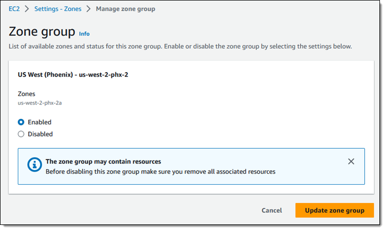




 Mikhail Smirnov is a Sr. Software Dev Engineer on the AWS Glue team and part of the AWS Glue DataBrew development team. Outside of work, his interests include learning to play guitar and traveling with his family.
 Gonzalo Herreros is a Sr. Big Data Architect on the AWS Glue team. Based on Dublin, Ireland, he helps customers succeed with big data solutions based on AWS Glue. On his spare time, he enjoys board games and cycling.






 Matt Nispel is an Enterprise Solutions Architect at AWS. He has more than 10 years of experience building cloud architectures for large enterprise companies. At AWS, Matt helps customers rearchitect their applications to take full advantage of the cloud. Matt lives in Minneapolis, Minnesota, and in his free time enjoys spending time with friends and family.
 Dan Dressel is a Senior Analytics Specialist Solutions Architect at AWS. He is passionate about databases, analytics, machine learning, and architecting solutions. In his spare time, he enjoys spending time with family, nature walking, and playing foosball.
 Ravi Kumar is a Senior Product Manager for Amazon EMR at Amazon Web Services.
 Kevin Wikant is a Software Development Engineer for Amazon EMR at Amazon Web Services.