Post Syndicated from The Atlantic original https://www.youtube.com/shorts/WxmT7HY-ris
Acemagic M1A PRO+ Review An AMD-Powered 128GB AI Mini PC
Post Syndicated from Ryan Smith original https://www.servethehome.com/acemagic-m1a-pro-review-an-amd-powered-128gb-ai-mini-pc/
We test the Acemagic M1A Pro+ a neat looking AI-focused mini PC with the AMD Ryzen AI Max+ 395 and 128GB of LPDDR5X memory
The post Acemagic M1A PRO+ Review An AMD-Powered 128GB AI Mini PC appeared first on ServeTheHome.
Избори 2026-та – обновени секции в чужбина, съвети за процеса на гласуване
Post Syndicated from Боян Юруков original https://yurukov.net/blog/2026/iz2026-sekcii-final/
На 19-ти април ще се проведат избори за Народно събрание. Остават само няколко дни и имаме на разположение по-малко секции в чужбини, в които да упражним правото си на глас, в сравнение с предишни избори. Сред 443-те места, където все пак ще има секции, около 1 от 5 имат променен адрес. Затова съветвам да сверите на картата дали при вашата ще има промени този път. Когато отворите избраната от Вас през линка, бихте могли да споделите в социалните мрежи, че ще гласувате там призовавайки и другите да го сторят.
Ето няколко важни неща, които трябва да знаете:
- Изборният ден започва в 7:00 сутринта местно време и свършва в 8:00 часа вечерта
- Може да гласува всеки български гражданин независимо дали е подал заявление или не. Тогава просто попълвате на място декларация по приложение 28, за да ви добавят в списъка.
- Гласува се с валидна българска лична карта или паспорт.
- Секциите отбелязани горе са актуални към 10-ти април. Възможно е в следващата седмица да има промени или корекции. Затова Ви препоръчвам да проверите преди изборния ден отново на картата и на сайта на МВнР.
- Независимо от отбелязаната в заявлението Ви секция, ако сте подали въобще такова, може да гласувате където и да е в чужбина.
- Извън България може да гласува всеки български гражданин независимо от обичайното му пребиваване. Това означава, че ако пътувате зад граница по работа или на почивка, може да упражните гласа си в близка до Вас секция. Отново, няма значение дали сте подавали заявление.
- Ако все пак сте в България по време на изборите, може да гласувате само по постоянен адрес. Тогава попълвате приложение 22, че не сте гласували в чужбина и са длъжни да Ви отбележат. Присъствате в списъка и след името Ви е отбелязано МВнР.
- В чужбина за Народно събрание има възможност да гласувате само за партия/коалиция. Възможност за преференции, каквито има в страната, отново няма да има след промени в Изборния кодекс в последния момент, за които писах преди. Запознайте се също с бюлетината.
- Препоръчвам да се гласува с машина, където това е възможно. На картата ще видите тази информация избирайки секция до вас. Гласуването с машина е по-бързо и гарантира, че гласът Ви ще бъде преброен и няма шанс да бъде отбелязан като невалиден.
- Препоръчвам да се гласува възможно най-рано, тъй като опитът показва, че с хартиено гласуване с напредването на деня стават струпвания на някои места. Ако имате съмнения и спомени за такива и имате друга близка секция с по-малко натоварване, препоръчваме да отидете там. На картата на Glasuvam.org може също да споделяте и преглеждате обратна връзка от други колко са чакали на това място.
Мейл с най-близките три секции изпратих на над 3100 абонирани за бюлетина на Glasuvam.org. Ако има промяна по някоя от секциите
Повече информация ще намерите на сайта на ЦИК и МВнР. Тази година ЦИК са добавили секция с често задавани въпроси. МВнР са направили своя карта със секциите, която може да заредите в Google Maps на телефона си, ако ви е по-удобно. Забелязах, че някои промени по адресите на секции не са въведени там 4 дни по-късно та съветвам да сверявате все пак с други източници. Такъв е случая с Нант, Франция и една от секциите в Бурса, Турция.

Тази година виждам, че и Facebook отново напомня за изборите на всички българи в страната и чужбина макар и само с линк към страницата на ЦИК.
Секциите с машинен вот
Заради намаления брой секции и утежнената ситуация с възможността на сънародниците ни зад граница да гласуват, реших да направя отделна карта визуализираща къде има секции с машинен вот. Аналогично преди две седмици направих карта с местата, където е имало секции преди, но сега няма да има заради новия Изборен кодекс.
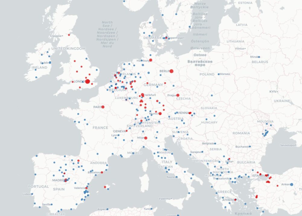
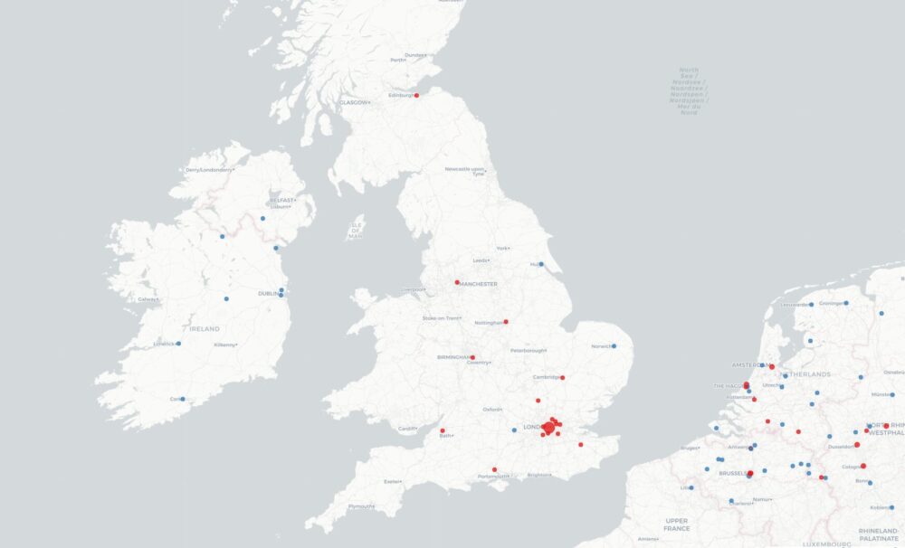
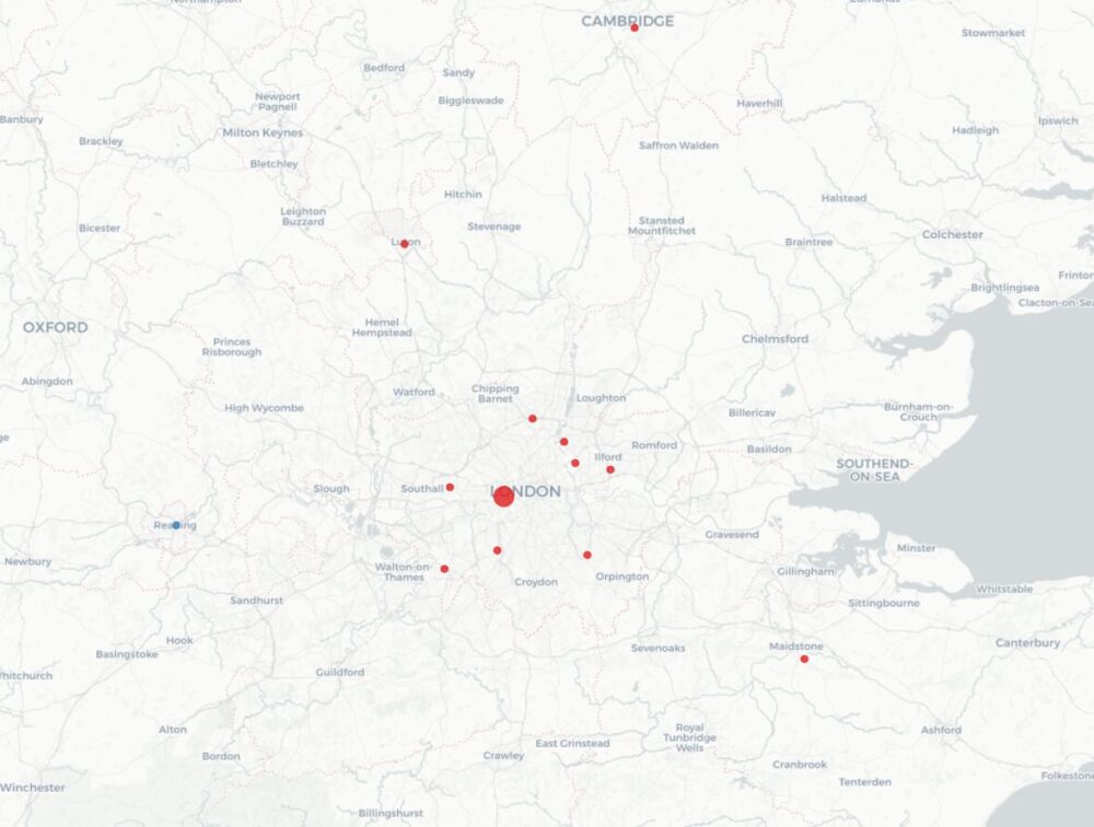
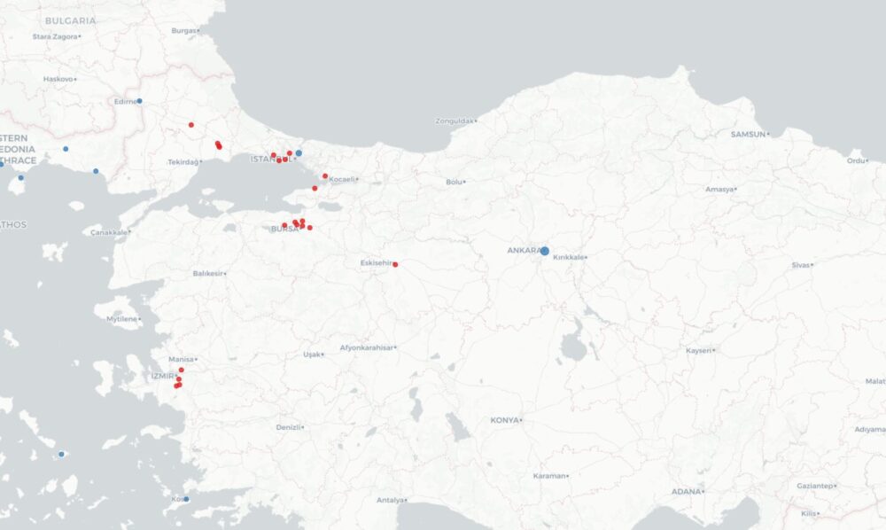

Както споменах по-горе, гласуването с машини не само е по-сигурно и спира редица изборни измами, но е и по-бързо. Вероятно затова ЦИК са решили да концентрират най-много машини във Великобритания и Турция, където натоварването е най-голямо. Тук ще намерите всички секции. В червено са тези, където има поне една секция с машинен вот. Размерът на точките показва колко секции има на това място. Същата информация ще намерите и като избирате отделни места за гласуване в картата със секциите.
Troubleshooting environment with AI analysis in AWS Elastic Beanstalk
Post Syndicated from Chandu Utlapalli original https://aws.amazon.com/blogs/devops/troubleshooting-environment-with-ai-analysis-in-aws-elastic-beanstalk/
Introduction
AWS Elastic Beanstalk simplifies the process of deploying and scaling web applications. You upload your code, and Elastic Beanstalk handles capacity provisioning, load balancing, auto scaling, and application health monitoring.
Elastic Beanstalk now offers AI Analysis to help troubleshoot environment health issues. When you request an analysis, Elastic Beanstalk triggers a script on the Amazon EC2 instance in your environment. The script collects environment events, health data, and instance logs, sends them to Amazon Bedrock for analysis, and uploads the results to Amazon S3. The result is a set of step-by-step troubleshooting recommendations tailored to your environment’s specific issues, helping you reduce mean time to resolution (MTTR).
In the Elastic Beanstalk console, the AI Analysis button appears on the environment overview page when your environment’s health status changes to Warning, Degraded, or Severe. AI analysis is also accessible from the logs page in the console, the AWS CLI, or the EB CLI.
Prerequisites
Before getting started, ensure that you have the following:
- An AWS account with access to AWS Elastic Beanstalk and Amazon Bedrock.
- A supported Elastic Beanstalk platform version – AI analysis is available on Amazon Linux 2 and AL2023 based platform versions released on or after February 16, 2026. Update your environment to a supported platform version if needed.
- Instance profile with required permissions – The managed policies AWSElasticBeanstalkWebTier, AWSElasticBeanstalkWorkerTier, and AWSElasticBeanstalkMulticontainerDocker now include the necessary permissions for AI analysis. Attach one or more of these managed policies to your environment’s instance profile based on your environment tier. If you use a custom instance profile, ensure it includes the following permissions:
bedrock:InvokeModelbedrock:ListFoundationModelselasticbeanstalk:DescribeEventselasticbeanstalk:DescribeEnvironmentHealth
- AWS CLI installed and configured with appropriate permissions. See Installing the AWS CLI.
- Anthropic use case details – AI analysis uses Anthropic Claude models through Amazon Bedrock. Anthropic requires you to submit a one-time use case details form before you can invoke their models. To submit this form, select an Anthropic model from the model catalog in the Amazon Bedrock console, or call the PutUseCaseForModelAccess API. You only need to do this once per AWS account. If you submit the form from the AWS Organizations management account, it automatically covers member accounts in the organization. For more information, see Access Amazon Bedrock foundation models.
- GovCloud Regions – If you are using AWS GovCloud (US) Regions, you must enable access to the latest Anthropic Claude Sonnet and/or Opus model in Amazon Bedrock before using AI analysis. For instructions on enabling model access in GovCloud Regions, see Manage access to Amazon Bedrock foundation models. For information about the latest available Anthropic Claude Sonnet and/or Opus model, see Supported Regions and models for inference profiles.
Solution Overview
In the following sections, we demonstrate how to use AI Analysis to diagnose a Node.js application that fails after a deployment.
- Create a working environment: Deploy a Node.js application to Elastic Beanstalk using the code snippets provided below.
- Break the environment: Update the application with code that requires missing environment variables. This causes the environment health status to transition to Degraded.
- Use AI Analysis: Request an AI Analysis from the Elastic Beanstalk console or the AWS CLI to identify the root cause of the health degradation.
- Apply the fix and verify: Apply the recommendations generated by AI Analysis and confirm that the environment health returns to Ok.
The following figure shows how AI Analysis works:
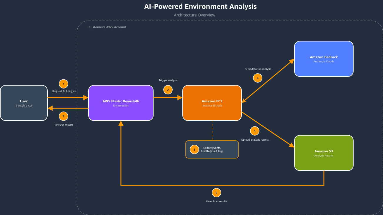
Figure 1 – AI Analysis architecture
- You initiate a request through the Elastic Beanstalk console (AI Analysis button) or the AWS CLI (RequestEnvironmentInfo API with InfoType set to “analyze”).
- Elastic Beanstalk collects environment data, analyzes it using Amazon Bedrock (a fully managed service that provides access to foundation models through API), and stores the results in Amazon S3.
- You retrieve the results through the console or the RetrieveEnvironmentInfo API using CLI.
Walkthrough
Follow the steps below to set up the sample application, break it, troubleshoot with AI Analysis, and restore the environment to a healthy state.
To try this feature, open your terminal and follow the steps below to create a sample Elastic Beanstalk environment. First, set the following variables. Replace the values with your own unique S3 bucket name and the latest Node.js solution stack for your region. To find the latest solution stack, run aws elasticbeanstalk list-available-solution-stacks.
S3_BUCKET="your-unique-bucket-name"

SOLUTION_STACK_NAME="64bit Amazon Linux 2023 v6.9.0 running Node.js 22"
Setting up the application
We use two versions of a simple Node.js application. The first version (v1-working) is a basic HTTP server that responds to requests successfully. The second version (v2-broken) introduces a dependency on environment variables that are not configured in the Elastic Beanstalk environment, simulating a common deployment issue.
Create a project directory:
mkdir test-app && cd test-app
Create the working application file (v1-working):
cat << 'EOF' > workingapp.js
const http = require('http');

const server = http.createServer((req, res) => {
    res.writeHead(200, { 'Content-Type': 'application/json' });
    res.end(JSON.stringify({ status: 'healthy', message: 'App is running' }));
});

const port = process.env.PORT || 8080;
server.listen(port, () => {
    console.log(`Server running on port ${port}`);
});
EOF
Create the broken application file (v2-broken):
cat << 'EOF' > brokenapp.js
const http = require('http');

// Application requires these environment variables to function
const VAR_1 = process.env.TEST_VARIABLE_1;
const VAR_2 = process.env.TEST_VARIABLE_2;
const VAR_3 = process.env.TEST_VARIABLE_3;

if (!VAR_1 || !VAR_2 || !VAR_3) {
    throw new Error(
        `Missing required environment variables. ` +
        `TEST_VARIABLE_1: ${VAR_1 ? 'set' : 'MISSING'}, ` +
        `TEST_VARIABLE_2: ${VAR_2 ? 'set' : 'MISSING'}, ` +
        `TEST_VARIABLE_3: ${VAR_3 ? 'set' : 'MISSING'}`
    );
}

const server = http.createServer((req, res) => {
    res.writeHead(200, { 'Content-Type': 'application/json' });
    res.end(JSON.stringify({ status: 'healthy', db: VAR_1 }));
});

const port = process.env.PORT || 8080;
server.listen(port, () => {
    console.log(`Server running on port ${port}`);
});
EOF
Create the package.json:
cat << 'EOF' > package.json
{
  "name": "test-app",
  "version": "1.0.0",
  "description": "Sample app that requires environment variables",
  "main": "app.js",
  "scripts": {
    "start": "node app.js"
  }
}
EOF
Create the working application source bundle:
cp workingapp.js app.js

zip -r nodejs-working-app.zip app.js package.json
Create the broken application source bundle:
cp brokenapp.js app.js

zip -r nodejs-broken-app.zip app.js package.json
Step 1: Create a working environment
First, create the Elastic Beanstalk application and deploy the working version.
Create an S3 bucket:
aws s3 mb s3://$S3_BUCKET --region us-east-1
Upload the working application source bundle:
aws s3 cp nodejs-working-app.zip s3://$S3_BUCKET/nodejs-working-app.zip
Create the Elastic Beanstalk application:
aws elasticbeanstalk create-application \
    --application-name test-app \
    --description "Test application" \
    --region us-east-1
Create the application version:
aws elasticbeanstalk create-application-version \
    --application-name test-app \
    --version-label v1-working \
    --source-bundle S3Bucket="$S3_BUCKET",S3Key="nodejs-working-app.zip" \
    --region us-east-1
Create the environment with the working version:
aws elasticbeanstalk create-environment \
    --application-name test-app \
    --environment-name test-app-env \
    --solution-stack-name "$SOLUTION_STACK_NAME" \
    --version-label v1-working \
    --option-settings \
        Namespace=aws:elasticbeanstalk:environment,OptionName=EnvironmentType,Value=SingleInstance \
        Namespace=aws:autoscaling:launchconfiguration,OptionName=IamInstanceProfile,Value=aws-elasticbeanstalk-ec2-role \
    --region us-east-1
Once your environment is created, verify the health:
aws elasticbeanstalk describe-environment-health \
    --environment-name test-app-env \
    --attribute-names All \
    --region us-east-1
Output:
{
    "EnvironmentName": "test-app-env",
    "HealthStatus": "Ok",
    "Status": "Ready",
    "Color": "Green",
    "Causes": [
        "Initialization completed 31 seconds ago and took 2 minutes."
    ],
    "ApplicationMetrics": {
        "RequestCount": 0
    },
    "InstancesHealth": {
        "NoData": 0,
        "Unknown": 0,
        "Pending": 0,
        "Ok": 1,
        "Info": 0,
        "Warning": 0,
        "Degraded": 0,
        "Severe": 0
    },
    "RefreshedAt": "2026-03-25T16:39:11Z"
}

Figure 2 – Environment health showing Ok (Green) status after initial deployment
Step 2: Break the environment
Now, deploy the broken version that requires missing environment variables.
Upload the broken version:
aws s3 cp nodejs-broken-app.zip s3://$S3_BUCKET/nodejs-broken-app.zip
Create the broken application version:
aws elasticbeanstalk create-application-version \
    --application-name test-app \
    --version-label v2-broken \
    --source-bundle S3Bucket="$S3_BUCKET",S3Key="nodejs-broken-app.zip" \
    --region us-east-1
Deploy the broken version:
aws elasticbeanstalk update-environment \
    --environment-name test-app-env \
    --version-label v2-broken \
    --region us-east-1
Within seconds of the deployment completing, the environment health transitions from Ok to Degraded:
aws elasticbeanstalk describe-environment-health \
    --environment-name test-app-env \
    --attribute-names All \
    --region us-east-1
Output:
{
    "EnvironmentName": "test-app-env",
    "HealthStatus": "Degraded",
    "Status": "Ready",
    "Color": "Red",
    "Causes": [
        "Impaired services on all instances."
    ],
    "ApplicationMetrics": {
        "RequestCount": 0
    },
    "InstancesHealth": {
        "NoData": 0,
        "Unknown": 0,
        "Pending": 0,
        "Ok": 0,
        "Info": 0,
        "Warning": 0,
        "Degraded": 0,
        "Severe": 1
    },
    "RefreshedAt": "2026-03-25T16:43:19Z"
}

Figure 3 – Environment health showing Degraded (Red) status with the AI Analysis button visible
Step 3: Use AI Analysis
Request AI analysis from the AWS CLI or the Elastic Beanstalk console. Both methods produce the same results. The CLI approach is useful for automation and scripting, while the console provides a visual workflow where you can view results directly on the environment page. We’ll cover both options below.
Using the AWS CLI
Request the analysis:
aws elasticbeanstalk request-environment-info \
    --environment-name test-app-env \
    --info-type analyze \
    --region us-east-1
Once the request environment operation is completed, retrieve the results:
aws elasticbeanstalk retrieve-environment-info \
    --environment-name test-app-env \
    --info-type analyze \
    --region us-east-1
The response includes an EnvironmentInfo array with a Message field containing a pre-signed S3 URL to the analysis results:
{
    "EnvironmentInfo": [
        {
            "InfoType": "analyze",
            "Ec2InstanceId": "i-1234567890abcdef0",
            "SampleTimestamp": "2026-03-20T20:49:22.763Z",
            "Message": "https://elasticbeanstalk-us-east-1-123456789012.s3.us-east-1.amazonaws.com/resources/environments/logs/analyze/..."
        }
    ]
}
Download and view the analysis:
ANALYSIS_URL=$(aws elasticbeanstalk retrieve-environment-info \
    --environment-name test-app-env \
    --info-type analyze \
    --region us-east-1 \
    --query 'sort_by(EnvironmentInfo, &SampleTimestamp)[-1].Message' \
    --output text)

curl -s "$ANALYSIS_URL"
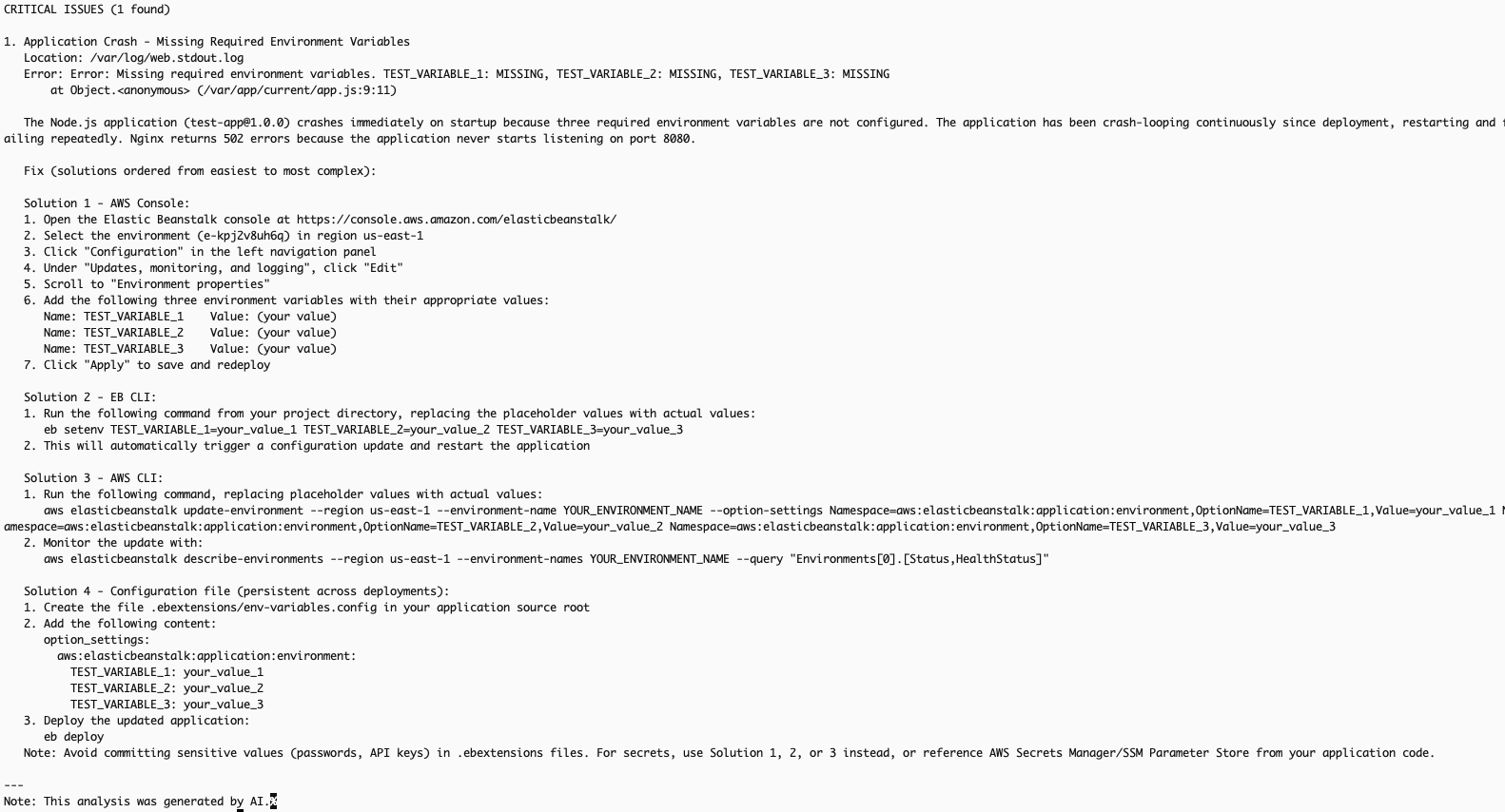
Figure 4 – AI analysis output retrieved via AWS CLI
Using the Elastic Beanstalk console
When your environment’s health status is Warning, Degraded, or Severe, the AI Analysis button appears in the environment overview section of the Elastic Beanstalk console.
- Navigate to the Elastic Beanstalk console.
- Select your environment (test-app-env).
- On the environment overview page, locate the AI Analysis button that appears when the health status indicates an issue.
- Choose AI Analysis to initiate the analysis.
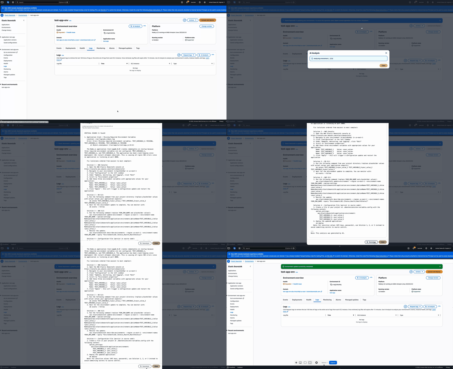
Video 1 – Requesting AI analysis from the Elastic Beanstalk console
If you want to restart the analysis workflow, you can click on the Reanalyze button to start a new analysis.
Step 4: Apply the fix and verify
The AI analysis identified that the application crashes because the environment does not have three required environment variables configured: TEST_VARIABLE_1, TEST_VARIABLE_2, and TEST_VARIABLE_3. As recommended by the AI analysis, set these environment variables to resolve the issue:
aws elasticbeanstalk update-environment \
    --environment-name test-app-env \
    --option-settings \
        Namespace=aws:elasticbeanstalk:application:environment,OptionName=TEST_VARIABLE_1,Value=value1 \
        Namespace=aws:elasticbeanstalk:application:environment,OptionName=TEST_VARIABLE_2,Value=value2 \
        Namespace=aws:elasticbeanstalk:application:environment,OptionName=TEST_VARIABLE_3,Value=value3 \
    --region us-east-1
After the environment update completes, the application starts successfully and the environment health returns to Ok:
aws elasticbeanstalk describe-environment-health \
    --environment-name test-app-env \
    --attribute-names All \
    --region us-east-1
Output:
{
    "EnvironmentName": "test-app-env",
    "HealthStatus": "Ok",
    "Status": "Ready",
    "Color": "Green",
    "Causes": [
        "Configuration update completed 72 seconds ago and took 54 seconds."
    ],
    "ApplicationMetrics": {
        "RequestCount": 0
    },
    "InstancesHealth": {
        "NoData": 0,
        "Unknown": 0,
        "Pending": 0,
        "Ok": 1,
        "Info": 0,
        "Warning": 0,
        "Degraded": 0,
        "Severe": 0
    },
    "RefreshedAt": "2026-03-25T17:42:47Z"
}

Figure 5 – Environment health restored to Ok (Green) after setting environment variables
Note: The steps in this walkthrough can also be performed using the EB CLI. For more information, see the EB CLI Command Reference.
Best practices
Consider these recommendations to get the most out of AI analysis for your environments.
- Use supported platform versions: Ensure your environment is running an Amazon Linux 2 or AL2023 platform version released on or after February 16, 2026. Update your platform if you don’t see the AI Analysis option.
- Implement fixes incrementally: If the analysis recommends multiple actions, implement them one at a time to isolate which change resolves the issue.
- Review data privacy considerations: The analysis sends environment events and logs to Amazon Bedrock running in your account. For more information about how Amazon Bedrock handles your data, see the Amazon Bedrock security documentation.
Cleaning up
Terminate the environment:
aws elasticbeanstalk terminate-environment \
    --environment-name test-app-env \
    --region us-east-1
Delete the application (after the environment is terminated):
aws elasticbeanstalk delete-application \
    --application-name test-app \
    --terminate-env-by-force \
    --region us-east-1
Delete the S3 bucket used for source bundles:
aws s3 rb s3://$S3_BUCKET --force --region us-east-1
Remove the local project directory:
rm -rf test-app
Conclusion
AI-powered environment analysis in AWS Elastic Beanstalk significantly reduces the time and effort required to diagnose environment health issues. Instead of manually parsing through log files and cross-referencing documentation, you can now get targeted, actionable recommendations with a click of the AI Analysis button in the console or an API call.
Whether you prefer using the Elastic Beanstalk console for visual workflows or the AWS CLI/EB CLI for scripting and automation, AI analysis provides a consistent experience that helps you quickly identify root causes and resolve issues.
To learn more about AI-powered environment analysis, see the AWS Elastic Beanstalk Developer Guide. To learn more about AWS Elastic Beanstalk, visit the product page.
About the Author
On Anthropic’s Mythos Preview and Project Glasswing
Post Syndicated from Bruce Schneier original https://www.schneier.com/blog/archives/2026/04/on-anthropics-mythos-preview-and-project-glasswing.html
The cybersecurity industry is obsessing over Anthropic’s new model, Claude Mythos Preview, and its effects on cybersecurity. Anthropic said that it is not releasing it to the general public because of its cyberattack capabilities, and has launched Project Glasswing to run the model against a whole slew of public domain and proprietary software, with the aim of finding and patching all the vulnerabilities before hackers get their hands on the model and exploit them.
There’s a lot here, and I hope to write something more considered in the coming week, but I want to make some quick observations.
One: This is very much a PR play by Anthropic—and it worked. Lots of reporters are breathlessly repeating Anthropic’s talking points, without engaging with them critically. OpenAI, presumably pissed that Anthropic’s new model has gotten so much positive press and wanting to grab some of the spotlight for itself, announced its model is just as scary, and won’t be released to the general public, either.
Two: These models do demonstrate an increased sophistication in their cyberattack capabilities. They write effective exploits—taking the vulnerabilities they find and operationalizing them—without human involvement. They can find more complex vulnerabilities: chaining together several memory corruption bugs, for example. And they can do more with one-shot prompting, without requiring orchestration and agent configuration infrastructure.
Three: Anthropic might have a good PR team, but the problem isn’t with Mythos Preview. The security company Aisle was able to replicate the vulnerabilities that Anthropic found, using older, cheaper, public models. But there is a difference between finding a vulnerability and turning it into an attack. This points to a current advantage to the defender. Finding for the purposes of fixing is easier for an AI than finding plus exploiting. This advantage is likely to shrink, as ever more powerful models become available to the general public.
Four: Everyone who is panicking about the ramifications of this is correct about the problem, even if we can’t predict the exact timeline. Maybe the sea change just happened, with the new models from Anthropic and OpenAI. Maybe it happened six months ago. Maybe it’ll happen in six months. It will happen—I have no doubt about it—and sooner than we are ready for. We can’t predict how much more these models will improve in general, but software seems to be a specialized language that is optimal for AIs.
A couple of weeks ago, I wrote about security in what I called “the age of instant software,” where AIs are superhumanly good at finding, exploiting, and patching vulnerabilities. I stand by everything I wrote there. The urgency is now greater than ever.
I was also part of a large team that wrote a “what to do now” report. The guidance is largely correct: We need to prepare for a world where zero-day exploits are dime-a-dozen, and lots of attackers suddenly have offensive capabilities that far outstrip their skills.
AWS Weekly Roundup: Claude Mythos Preview in Amazon Bedrock, AWS Agent Registry, and more (April 13, 2026)
Post Syndicated from Micah Walter original https://aws.amazon.com/blogs/aws/aws-weekly-roundup-claude-mythos-preview-in-amazon-bedrock-aws-agent-registry-and-more-april-13-2026/
In my last Week in Review post, I mentioned how much time I’ve been spending on AI-Driven Development Lifecycle (AI-DLC) workshops with customers this year. A common theme in those sessions is the need for better cost visibility. Teams are moving fast with AI, but as they go from experimenting to full production, finance and leadership really need to know who is using which resources and at what cost. That’s why I was so excited to see the launch of Amazon Bedrock new support for cost allocation by IAM user and role this week. This lets you tag IAM principals with attributes like team or cost center and then activate those tags in your Billing and Cost Management console. The resulting cost data flows into AWS Cost Explorer and the detailed Cost and Usage Report, giving you a clear line of sight into model inference spending. Whether you’re scaling agents across teams, tracking foundation model use by department, or running tools like Claude Code on Amazon Bedrock, this new feature is a game changer for tracking and managing your AI investments. You can get all the details on setting this up in the IAM principal cost allocation documentation.
Now, let’s get into this week’s AWS news…
Headlines
Amazon Bedrock now offers Claude Mythos Preview Anthropic’s most sophisticated AI model to date is now available on Amazon Bedrock as a gated research preview through Project Glasswing. Claude Mythos introduces a new model class focused on cybersecurity, capable of identifying sophisticated security vulnerabilities in software, analyzing large codebases, and delivering state of the art performance across cybersecurity, coding, and complex reasoning tasks. Security teams can use it to discover and address vulnerabilities in critical software before threats emerge. Access is currently limited to allowlisted organizations, with Anthropic and AWS prioritizing internet critical companies and open source maintainers.
AWS Agent Registry for centralized agent discovery and governance now in preview AWS launched Agent Registry through Amazon Bedrock AgentCore, providing organizations with a private catalog for discovering and managing AI agents, tools, skills, MCP servers, and custom resources. The registry helps teams locate existing capabilities rather than duplicating them, with semantic and keyword search, approval workflows, and CloudTrail audit trails. It is accessible via the AgentCore Console, AWS CLI, SDK, and as an MCP server queryable from IDEs.
Last week’s launches
Here are some launches and updates from this past week that caught my attention:
- Announcing Amazon S3 Files, making S3 buckets accessible as file systems — Amazon S3 Files transforms S3 buckets into shared file systems that connect any AWS compute resource directly with your S3 data. Built on Amazon EFS technology, it delivers full file system semantics with low latency performance, caching actively used data and providing multiple terabytes per second of aggregate read throughput. Applications can access S3 data through both file system and S3 APIs simultaneously without code modifications or data migration.
- Amazon OpenSearch Service supports Managed Prometheus and agent tracing —Amazon OpenSearch Service now provides a unified observability platform that consolidates metrics, logs, traces, and AI agent tracing into a single interface. The update includes native Prometheus integration with direct PromQL query support, RED metrics monitoring, and OpenTelemetry GenAI semantic convention support for LLM execution visibility. Operations teams can correlate slow traces to logs and overlay Prometheus metrics on dashboards without switching between tools.
- Amazon WorkSpaces Advisor now available for AI powered troubleshooting— AWS launched Amazon WorkSpaces Advisor, an AI powered administrative tool that uses generative AI to help IT administrators troubleshoot Amazon WorkSpaces Personal deployments. It analyzes WorkSpace configurations, detects problems automatically, and provides actionable recommendations to restore service and optimize performance.
- Amazon Braket adds support for Rigetti’s 108 qubit Cepheus QPU — Amazon Braket now offers access to Rigetti’s Cepheus-1-108Q device, the first 100+ qubit superconducting quantum processor on the platform. The modular design features twelve 9 qubit chiplets with CZ gates that offer enhanced resilience to phase errors. It supports multiple frameworks including Braket SDK, Qiskit, CUDA-Q, and Pennylane, with pulse level control for researchers.
For a full list of AWS announcements, be sure to keep an eye on the What’s New with AWS page.
Other AWS news
Here are some additional posts and resources that you might find interesting:
- Building automated AWS Regional availability checks with Amazon S3— Storage blog post on implementing automated systems for monitoring service availability across AWS regions using Amazon S3 as core infrastructure.
- Understanding Amazon Bedrock model lifecycle — Machine learning blog post that walks through the stages foundation models go through in Bedrock from availability through deprecation, helping teams plan for model updates and manage version dependencies in production.
- Building memory intensive apps with AWS Lambda managed instances — Compute blog post exploring how Lambda managed instances extend the platform beyond lightweight workloads to support memory intensive applications while maintaining serverless benefits.
- Deploy OpenClaw on AWS: Choose the right options for your AI workload — Builder Center guide comparing four AWS deployment options for OpenClaw: Amazon Lightsail for individual developers, Amazon EC2 for startups needing deeper AWS integration, Amazon Bedrock AgentCore for serverless multiuser scenarios, and Amazon EKS for enterprises requiring VM level isolation and advanced orchestration.
- We’re bringing back the Kiro startup credits program — Kiro is relaunching its startup credits initiative, offering eligible early stage companies complimentary access to Kiro Pro+ for up to one year. The three tier program (Starter, Growth, Scale) provides 2 to 30 users based on team size, with rolling applications accepted globally.
Upcoming AWS events
Check your calendar and sign up for upcoming AWS events:
- What’s Next with AWS (April 28, Virtual) Join this livestream at 9am PT for a candid discussion about how agentic AI is transforming how businesses operate. Featuring AWS CEO Matt Garman, SVP Colleen Aubrey, and OpenAI leaders discussing emerging agent capabilities, Amazon’s internal experiences, and new agentic solutions and platform capabilities.
Browse here for upcoming AWS led in person and virtual events, startup events, and developer focused events.
That’s all for this week. Check back next Monday for another Weekly Roundup!
~ micah
[$] Development statistics for the 7.0 kernel
Post Syndicated from corbet original https://lwn.net/Articles/1066723/
Linus Torvalds released the 7.0 kernel as
expected on April 12, ending a relatively busy development cycle. The
7.0 release brings a large number of interesting changes; see the LWN
merge-window summaries (part 1, part 2) for all the details. Here,
instead, comes our traditional look at where those changes came from and
who supported that work.
How to use Parquet Column Indexes with Amazon Athena
Post Syndicated from Matt Wong original https://aws.amazon.com/blogs/big-data/how-to-use-parquet-column-indexes-with-amazon-athena/
Amazon Athena recently added support for reading Parquet Column Indexes in Apache Iceberg tables on November 21, 2025. With this optimization, Athena can perform page-level data pruning to skip unnecessary data within Parquet row groups, potentially reducing the amount of data scanned and improving query runtime for queries with selective filters. For data teams, this may help enable faster insights and help reduce costs when analyzing large-scale data lakes.
Data teams building data lakes often choose Apache Iceberg for its ACID transactions, schema evolution, and metadata management capabilities. Athena is a serverless query engine that allows you to query Amazon S3-based data lakes using SQL, and you don’t need to manage infrastructure. Based on the type of data and query logic, Athena can apply multiple query optimizations to improve performance and reduce costs.
In this blog post, we use Athena and Amazon SageMaker Unified Studio to explore Parquet Column Indexes and demonstrate how they can improve Iceberg query performance. We explain what Parquet Column Indexes are, demonstrate their performance benefits, and show you how to use them in your applications.
Overview of Parquet Column Indexes
Parquet Column Indexes store metadata that query engines can use to skip irrelevant data with greater precision than row group statistics alone. To understand how they work, consider how data is structured within Parquet files and how engines like Athena process them.
Parquet files organize data hierarchically by dividing data into row groups (typically 128-512 MB each) and further subdividing them into pages (typically 1 MB each). Traditionally, Parquet maintains metadata on the contents of each row group level in the form of min/max statistics, allowing engines like Athena to skip row groups that don’t satisfy query predicates. Although this approach reduces the bytes scanned and query runtime, it has limitations. If even a single page within a row group overlaps with the values you are searching for, Athena scans all pages within the row group.
Parquet Column Indexes help address this problem by storing page-level min/max statistics in the Parquet file footer. Row group statistics provide coarse-grained filtering, but Parquet Column Indexes enable finer-grained filtering by allowing query engines like Athena to skip individual pages within a row group. Consider a Parquet file with a single row group containing 5 pages for a column. The row group has min/max statistics of (1, 20), and each page for that column has the following min/max statistics.
When Athena runs a query filtering for values equal to 2, it first checks the row group statistics and confirms that 2 falls within the range (1, 20). Athena will then plan to scan the pages within that row group. Without Parquet Column Indexes, Athena scans each of the 5 pages in the row group. With Parquet Column Indexes, Athena examines the page-level statistics and determines that only page-0 and page-1 need to be read, skipping the remaining 3 pages.
How to use Parquet Column Indexes with Athena
Athena uses Parquet Column Indexes based on table type:
- Amazon S3 Tables: Athena automatically uses Parquet Column Indexes by default when they are present.
- Iceberg tables in S3 general purpose buckets: Athena does not use Parquet Column Indexes by default. To allow Athena to use Parquet Column Indexes, add an AWS Glue table property named
use_iceberg_parquet_column_indexand set it totrue. Use the AWS Glue console or AWS Glue UpdateTable API to perform these actions.
Read more about how to use this feature in Use Parquet column indexing.
Measuring Athena performance gains when using Parquet Column Indexes
Now that we understand what Parquet Column Indexes are, we’ll demonstrate the performance benefits of using Parquet Column Indexes by analyzing the catalog_sales table from a 3TB TPC-DS dataset. This table contains ecommerce transaction data including order dates, sales amounts, customer IDs, and product information. This dataset is a good proxy for the types of business analysis that you might perform on your own data, such as identifying sales trends, analyzing customer purchasing patterns, and calculating revenue metrics. We compare query execution statistics with and without Parquet Column Indexes to quantify the performance improvement.
Prerequisites
Before you begin, you must have the following resources:
- A SageMaker Unified Studio IAM-based domain.
- An Execution IAM Role configured within the SageMaker Unified Studio IAM-based domain with access to S3, AWS Glue Data Catalog, and Athena.
- An S3 bucket in your account to store Iceberg table data and Athena query results.
Create catalog_sales Iceberg table
Complete the following steps using SageMaker Unified Studio notebooks. There, you can use SageMaker Unified Studio’s multi-dialect notebook functionality to work with your data using the Athena SQL and Spark engines. To create a catalog_sales Iceberg table in your account, follow these steps:
- Navigate to Amazon SageMaker in the AWS Management Console and choose Open under Get started with Amazon SageMaker Unified Studio.
- From the side navigation, select Notebooks and choose Create Notebook. The subsequent steps in this post will execute scripts in this notebook.
- Create a new SQL cell in the notebook and set the connection type to Athena (Spark). Execute the following query to create a database for the tables in this post.
- Create a new SQL cell in the notebook and verify the connection type is Athena (Spark). Execute the following query to create a Hive table pointing to the location of the TPC-DS
catalog_salestable data at the public S3 bucket. - Create a new SQL cell in the notebook and verify the connection type is Athena (Spark). Execute the following query to add the Hive partitions to the AWS Glue metadata.
- Create a new SQL cell in the notebook and verify the connection type is Athena (Spark). Replace
s3://amzn-s3-demo-bucket/athena_parquet_column_index_blog/catalog_sales/with the S3 URI where you want to store your Iceberg table data, then execute the following query to create thecatalog_salesIceberg table from the Hive table. - Create a new SQL cell in the notebook and verify the connection type is Athena (Spark). Execute the following query to delete the
catalog_sales_hivetable, which was only needed to create thecatalog_salesIceberg table.
Run an Athena query without Parquet Column Indexes
After creating the catalog_sales Iceberg table in the preceding steps, we run a simple query that analyzes shipping delays of the top 10 most ordered items. This type of analysis could be critical for ecommerce and retail operations. By identifying which popular items experience the greatest delays, fulfillment teams can focus resources where they matter most. For example, you can adjust inventory placement, change warehouse assignments, or address carrier issues. Additionally, popular items with significant shipping delays are more likely to result in order cancellations or returns, so proactively identifying these issues helps protect revenue.
Additionally, this query is a good candidate for demonstrating the effectiveness of using Parquet Column Indexes because it has a selective filter predicate on a single column cs_item_sk. When Athena executes this query, it first identifies row groups whose min/max ranges overlap with the top 10 most ordered items. Without using Parquet Column Indexes, Athena has to scan every page of data within those matched row groups. However, when using Parquet Column Indexes, Athena can prune data further by skipping individual pages within those row groups whose min/max ranges do not overlap with the ids. Complete the following steps to establish baseline query performance when Athena does not use Parquet Column Indexes during the query.
- Create a new Python cell in the notebook. Replace
s3://amzn-s3-demo-bucket/athena_parquet_column_index_blog/query_results/with the S3 URI where you want to store your Athena query results, then execute the following script. Note the runtime and bytes scanned that will be printed. The script will run the query five times with query result reuse disabled and chooses the minimum runtime and the corresponding bytes scanned among those iterations. See our numbers in the Run Athena query with Parquet Column Indexes section.
Sort the catalog_sales table
Before rerunning the query with Athena using Parquet Column Indexes, you need to sort the catalog_sales table by the cs_item_sk column. In the preceding query, there is a dynamic filter as a subquery on the cs_item_sk column:
When executing this query, Athena pushes down the filter predicate to the data source level, fetching only rows that match the top 10 most ordered items. To maximize page pruning with Parquet Column Indexes, rows with the same cs_item_sk values should be stored near each other in the Parquet file. Without sorting, matching values could be scattered across many pages, forcing Athena to read more data. Sorting the table by cs_item_sk clusters similar values together, enabling Athena to read fewer pages.
Let’s examine the Parquet Column Indexes in one of the Parquet files to understand how the data in the catalog_sales table is currently organized. First, download the Parquet file from the cs_sold_date_sk = 2450815 partition and install the open-source parquet-cli tool on your local machine. Replace <local-path-to-parquet-file> with the path to the downloaded Parquet file, then run the following command on your local machine:
This displays Parquet Column Indexes for all columns. For brevity, only the first 11 pages of the cs_item_sk column from the first row group are shown in the following example:
Notice that nearly every page contains a wide range of values. This overlap means Athena cannot eliminate pages when filtering with Parquet Column Indexes on cs_item_sk. For example, searching for cs_item_sk = 100 requires scanning each of the 11 pages because the value 100 falls within every page’s min/max range. With this overlap, enabling Athena to use Parquet Column Indexes would provide no performance benefit. Sorting the data by cs_item_sk eliminates this overlap, creating distinct, non-overlapping ranges for each page. To make Parquet Column Indexes more effective, sort the table by completing the following step:
- Create a new SQL cell in the notebook and verify the connection type is Athena (Spark). Execute the query to sort the
cs_item_skcolumn values of thecatalog_salestable in ascending order and to put all the null values in the last few Parquet pages. New Iceberg data files will be generated from this query.
Running the parquet column-index command on the sorted data file from the cs_sold_date_sk = 2450815 partition shows that the Parquet Column Indexes are now sorted and have non-overlapping ranges. The first 11 pages of the cs_item_sk column from the first row group are shown in the following example:
Now when searching for cs_item_sk = 100, Athena only needs to read page-0, skipping the remaining 10 pages entirely.
Run Athena query with Parquet Column Indexes
Now that the data is sorted to eliminate overlapping pages within the row groups for the cs_item_sk column, we run two experiments on the sorted data. The first measures the impact of sorting alone, and the second measures the combined effect of sorting with Parquet Column Indexes.
- Create a new Python cell in the notebook. Execute the same script in the section Run Athena query without Parquet Column Indexes and take note of the query runtime and bytes scanned results. This measures the performance of querying sorted data without using Parquet Column Indexes.
- Create a new Python cell in the notebook. Execute the following Python script to set the
use_iceberg_parquet_column_indextable property totruefor thecatalog_salestable in the AWS Glue Data Catalog. - Create a new Python cell in the notebook. Execute the same script in the section Run Athena query without Parquet Column Indexes and take note of the query runtime and bytes scanned results. This measures the performance of querying sorted data using Parquet Column Indexes.
Athena query time and bytes scanned improvement
The following table summarizes the results from each experiment. The percentage improvements for the sorted experiments are measured against the unsorted baseline.
| Experiment | Runtime (sec) | Bytes Scanned (GB) |
| Unsorted without Parquet Column Indexes | 20.6 | 45.2 |
| Sorted without Parquet Column Indexes | 15.4 (25.2% faster) | 27.8 (38.5% fewer bytes) |
| Sorted with Parquet Column Indexes | 10.3 (50.0% faster) | 13.0 (71.2% fewer bytes) |
Recommendations
To maximize Athena’s ability to use Parquet Column Indexes and achieve optimal query performance, we recommend the following.
- Sort data by frequently filtered columns. This allows Athena to efficiently read Parquet Column Indexes and skip irrelevant pages, potentially reducing scan time. When data is sorted by a filter column, similar values are clustered together within pages. Because Parquet Column Indexes store min/max values for each page, Athena can quickly determine which pages contain matching values and skip the rest.
- Sort data by high-cardinality columns. This creates distinct value ranges between pages, maximizing the opportunity for Athena to skip pages during query execution. High-cardinality (many distinct values) columns produce non-overlapping min/max ranges across pages, allowing Athena to more effectively filter out irrelevant pages. In contrast, low-cardinality columns such as boolean or status fields result in overlapping ranges across many pages, reducing the number of skipped pages.
Clean up
When you have finished the steps in this post, complete the following cleanup actions to avoid incurring ongoing charges:
- Create a new SQL cell in the notebook and set the connection type to Athena (Spark). Execute the following command to drop the
parquet_column_index_blogdatabase and thecatalog_salestable. - Delete the Iceberg table data and the Athena query results from your S3 bucket.
- Delete the SageMaker Unified Studio IAM-based domain if it is no longer needed.
Conclusion
In this post, we showed you how Athena uses Parquet Column Indexes to speed up queries and reduce the number of bytes scanned. By using Parquet Column Indexes, Athena can skip irrelevant data pages to improve query performance, especially for queries with selective filters on sorted data. Refer to Optimize Iceberg tables to learn more about this feature and try it out on your own queries.
About the Author
Implementing Kerberos authentication for Apache Spark jobs on Amazon EMR on EKS to access a Kerberos-enabled Hive Metastore
Post Syndicated from Krishna Kumar Venkateswaran original https://aws.amazon.com/blogs/big-data/implementing-kerberos-authentication-for-apache-spark-jobs-on-amazon-emr-on-eks-to-access-a-kerberos-enabled-hive-metastore/
Many organizations run their Apache Spark analytics platforms on Amazon EMR on Amazon Elastic Compute Cloud (Amazon EC2), using Kerberos authentication to secure connectivity between Spark jobs and a centralized shared Apache Hive Metastore (HMS). With Amazon EMR on Amazon EKS, they gained a new option for running Spark jobs with the benefits of Kubernetes-based container orchestration, improved resource utilization, and faster job startup times. However, an HMS deployment supports only one authentication mechanism at a time. This means that they must configure Kerberos authentication for their Spark jobs on Amazon EMR on EKS to connect to the existing Kerberos-enabled HMS.
In this post, we show how to configure Kerberos authentication for Spark jobs on Amazon EMR on EKS, authenticating against a Kerberos-enabled HMS so you can run both Amazon EMR on EC2 and Amazon EMR on EKS workloads against a single, secure HMS deployment.
Overview of solution
Consider an enterprise data platform team that’s been running Spark jobs on Amazon EMR on EC2 for several years. Their architecture includes a Kerberos-enabled standalone HMS that serves as the centralized data catalog, with Microsoft Active Directory functioning as the Key Distribution Center (KDC). As the team evaluates Amazon EMR on EKS for new workloads, their existing HMS must continue serving Amazon EMR on EC2, with both authenticating through the same Kerberos infrastructure. To address this, the platform team must configure their Spark jobs running on Amazon EMR on EKS to authenticate with the same KDC. This is so they can obtain valid Kerberos tickets and establish authenticated connections to the HMS while maintaining a unified security posture across their data platform.
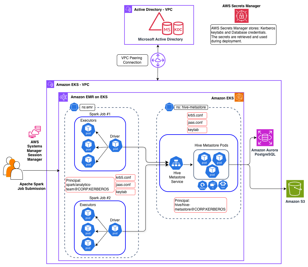
Scope of Kerberos in this solution
Kerberos authentication in this solution secures the connection between Spark jobs and the HMS. Other components in the architecture use AWS and Kubernetes security mechanisms instead.
Solution architecture
Our solution implements Kerberos authentication to secure the connection between Spark jobs and the HMS. The architecture spans two Amazon Virtual Private Clouds (Amazon VPCs) connected using VPC peering, with distinct components handling identity management, compute, and metadata services.
Identity and Authentication layer
A self-managed Microsoft Active Directory Domain Controller is deployed in a dedicated VPC and serves as the KDC for Kerberos authentication. The Active Directory server hosts service principals for both the HMS service and Spark jobs. This separate VPC deployment mirrors real-world enterprise architectures where Active Directory is typically managed by identity teams in their own network boundary, whether on-premises or in AWS.
Data Platform layer
The data platform components reside in a separate VPC and includes an EKS cluster that hosts both the HMS service and Amazon EMR on EKS based Spark jobs persisting data in an Amazon Simple Storage Service (Amazon S3) bucket.
Hive Metastore service
The HMS is deployed in the EKS hive-metastore namespace and simulates a pre-existing, standalone Kerberos-enabled HMS, a common enterprise pattern where HMS is managed independently of any data processing platform. You can learn more about other enterprise design patterns in the post Design patterns for implementing Hive Metastore for Amazon EMR or EKS. The HMS service authenticates with the KDC using its service principal and keytab mounted from a Kubernetes secret.
Apache Spark Execution layer
Apache Spark jobs are deployed using the Spark Operator on EKS. The Spark driver and executor pods are configured with Kerberos credentials through mounted ConfigMaps containing krb5.conf and jaas.conf, along with keytab files from Kubernetes secrets. When a Spark job must access Hive tables, the driver authenticates with the KDC and establishes a secure Simple Authentication and Security Layer (SASL) connection to the HMS.
Authentication flow
The HMS runs as a long-running Kubernetes service that must be deployed and authenticated before Spark jobs can connect.
During HMS deployment:
- HMS pod validates its Kerberos configuration.
krb5.confandjaas.confare mounted fromConfigMaps - Service authenticates with KDC using its principal
hive/hive-metastore-svc.hive-metastore.svc.cluster.local@CORP.KERBEROS keytabis mounted from Kubernetes secret for credential access- Secure Thrift endpoint is established on
port 9083with SASL authentication enabled
When a Spark job must interact with the HMS:
- Spark job submission:
- User submits Spark job through Spark Operator
- Driver and executor pods are created with Kerberos configuration mounted as volumes
krb5.confConfigMap provides KDC connection details including realm and server addressesjaas.confConfigMap specifies a login module configuration withkeytabpath and principalKeytabsecret contains encrypted credentials for Spark service principalspark/[email protected]
- Authentication and connection:
- Spark driver authenticates with KDC using its principal and
keytabto obtain a Ticket Granting Ticket (TGT) - When connecting to HMS, Spark requests a service ticket from the KDC for the HMS principal
hive/hive-metastore-svc.hive-metastore.svc.cluster.local@CORP.KERBEROS - KDC issues a service ticket encrypted with HMS’s secret key
- Spark presents this service TGT to HMS over the Thrift connection on
port 9083 - HMS decrypts the ticket using its
keytab, verifies Spark’s identity, and establishes the authenticated SASL session - Executor pods use the same configuration for authenticated operations
- Spark driver authenticates with KDC using its principal and
- Data access:
- Authenticated Spark job queries HMS for table metadata
- HMS validates Kerberos tickets before serving metadata requests
- Spark accesses underlying data in Amazon S3 using IRSA
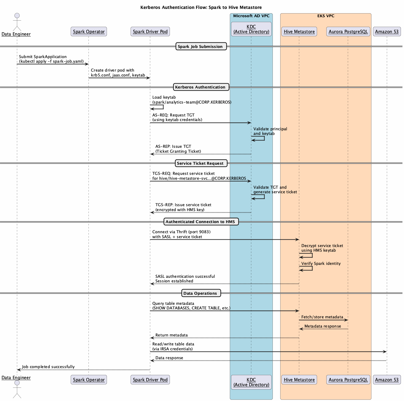
Implementation workflow
The implementation involves three key stakeholders working together to establish the Kerberos-enabled communication:
Microsoft Active Directory Administrator
The Active Directory Administrator creates service accounts that are used for HMS and Spark jobs. This involves setting up the service principal names using the setspn utility and generating keytab files using ktpass for secure credential storage. The administrator configures the appropriate Active Directory permissions and Kerberos AES256 encryption type. Finally, the keytab files are uploaded to AWS Secrets Manager for secure distribution to Kubernetes workloads.
Data Platform Team
The platform team handles the Amazon EMR on EKS and Kubernetes configurations. They retrieve keytabs from Secrets Manager and create Kubernetes secrets for the workloads. They configure Helm charts for HMS deployment with Kerberos settings and set up ConfigMaps for krb5.conf, jaas.conf, and core-site.xml.
Data Engineering Operations
Data engineers submit jobs using the configured service account with Kerberos authentication. They monitor job execution and verify authenticated access to HMS.
Deploy the solution
In the remainder of this post, you will explore the implementation details for this solution. You can find the sample code in the AWS Samples GitHub repository. For additional details, including verification steps for each deployment stage, refer to the README in the repository.
Prerequisites
Before you deploy this solution, make sure that the following prerequisites are in place:
- Access to a valid AWS account and permission to create AWS resources.
- The AWS Command Line Interface (AWS CLI) is installed on your local machine.
- Git, Docker, eksctl, kubectl, Helm, envsubst, jq, and yq utilities are installed on your local machine.
- Familiarity with Kerberos, Apache Hive Metastore (HMS), Apache Spark, Kubernetes, Amazon EKS, and Amazon EMR on Amazon EKS.
Clone the repository and set up environment variables
Clone the repository to your local machine and set the two environment variables. Replace <AWS_REGION> with the AWS Region where you want to deploy these resources.
Setup Microsoft Active Directory infrastructure
In this section, we deploy a self-managed Microsoft Active Directory with KDC on a Windows Server EC2 instance into a dedicated VPC. This is an intentionally minimal implementation highlighting only the key components required for this blog post.
Setup EKS infrastructure
This section provisions the Amazon EMR on EKS infrastructure stack, including VPC, EKS cluster, Amazon Aurora PostgreSQL database, Amazon Elastic Container Registry (Amazon ECR), Amazon S3, Amazon EMR on EKS virtual clusters and the Spark Operator. Run the following script.
Set up VPC peering
This section establishes network connectivity between the Active Directory VPC and EKS VPC for Kerberos authentication. Run the following script:
Deploy Hive Metastore with Kerberos authentication
This section deploys a Kerberos-enabled HMS service on the EKS cluster. Complete the following steps:
- Create Kerberos Service Principal for HMS service
- Deploy HMS service with Kerberos authentication
Set up Amazon EMR on Amazon EKS with Kerberos authentication
This section configures Spark jobs to authenticate with Kerberos-enabled HMS. This involves creating service principles for Spark jobs and generating the necessary configuration files. Complete the following steps:
- Create Service Principal for Spark jobs
- Generate Kerberos configurations for Spark jobs
Submit Spark jobs
This section verifies Kerberos authentication by running a Spark job that connects to the Kerberized HMS. Complete the following steps:
- Submit the test Spark job
- Monitor job execution
- Verify Kerberos authentication and HMS connection
The logs should confirm successful authentication, along with a listing of sample databases and tables.
Understanding Kerberos configuration
The HMS requires specific configuration parameters to enable Kerberos authentication, applied through the previously mentioned steps. The key configurations are outlined in the following section.
HMS configuration (metastore-site.xml)
The following configurations are added to metastore-site.xml file.
| Setting | Value | Purpose |
hive.metastore.sasl.enabled |
true | Enable SASL authentication |
hive.metastore.kerberos.principal |
hive/hive-metastore-svc.hive-metastore.svc.cluster.local@CORP.KERBEROS |
HMS service principal |
hive.metastore.kerberos.keytab.file |
/etc/security/keytab/hive.keytab |
Keytab path |
Hadoop security (core-site.xml)
The following configurations are added to the core-site.xml file.
| Setting | Value |
hadoop.security.authentication |
kerberos |
hadoop.security.authorization |
true |
Spark configuration
| Setting | Value | Purpose |
spark.security.credentials.kerberos.enabled |
true | Enable Kerberos for Spark |
spark.hadoop.hive.metastore.sasl.enabled |
true | SASL for HMS connection |
spark.kerberos.principal |
spark/[email protected] |
Spark service principal |
spark.kerberos.keytab |
local:///etc/security/keytab/analytics-team.keytab |
Keytab path |
Shared Kerberos files
Both HMS and Spark pods mount two common Kerberos configuration files: krb5.conf and jaas.conf, using ConfigMaps and Kubernetes secrets. The krb5.conf file is identical across both services and defines how each component connects to the KDC. The jaas.conf file follows the same structure but differs in the principal and keytab path for each service.
krb5Configuration
For more information, see the online documentation for krb5.conf.
- JAAS configuration
Additional security considerations
This post focuses on core Kerberos authentication mechanics between Spark and HMS. We recommend two additional security hardening steps based on your organization’s security posture and compliance requirements.
Protecting Keytabs at Rest with AWS KMS Envelope Encryption
Keytabs stored as Kubernetes Secrets are only base64-encoded by default, not encrypted at rest. We recommend enabling EKS envelope encryption using an AWS Key Management Service (AWS KMS) customer managed key. With envelope encryption, secret data is encrypted with a Data Encryption Key (DEK), which is encrypted by your customer managed key. This protects keytab content even if the etcd datastore is compromised. To enable this on an existing EKS cluster:
Refer to the Amazon EKS documentation on envelope encryption for full setup guidance.
Encrypting the Thrift Data Channel with TLS
SASL with Kerberos provides mutual authentication but doesn’t automatically encrypt data over the Thrift connection. Many deployments default to auth QoP, leaving the data channel unencrypted. We recommend either:
- Set SASL QoP to auth-conf — enables SASL-layer encryption using Kerberos session keys
- Layer TLS over Thrift (preferred) — enables transport-level encryption using modern cipher suites
Enabling TLS on HiveServer2 / Hive Metastore Thrift:
Refer to the Hive SSL/TLS configuration documentation for full details.
Cleaning up
To avoid incurring future charges, clean up all provisioned resources during this setup by executing the following cleanup script.
Conclusion
In this post, we demonstrated how to implement Kerberos authentication for Amazon EMR on EKS to securely connect to a Kerberos-enabled HMS. This solution addresses a common challenge faced by organizations with existing Kerberos-enabled HMS deployments who want to adopt Amazon EMR on EKS while maintaining their Kerberos-enabled security posture.
This pattern applies whether you’re migrating from on-premises Hadoop, running hybrid Amazon EMR on EC2 or Amazon EMR on EKS environments, or building a new cloud-native platform. Any scenario where Spark jobs on Kerberos must authenticate with a shared, Kerberos-enabled HMS.
You can use this post as a starting point to implement this pattern and extend it further to suit your organization’s data platform needs.
About the authors
[$] A build system aimed at license compliance
Post Syndicated from jake original https://lwn.net/Articles/1066103/
The OpenWrt One is a
router powered by the open-source firmware from the OpenWrt project; it was also the
subject of a keynote at SCALE in 2025
given by Denver Gingerich of the Software Freedom Conservancy (SFC),
which played a big role in developing the router. Gingerich returned to
the conference in
2026 to talk about the build system used by the OpenWrt One, which is
focused on creating the needed binaries, naturally, but doing so in a way
that makes it easy to comply with the licenses of the underlying code.
That makes good sense for a project of this sort—and for a talk given by
the director of compliance at SFC.
Servo now on crates.io
Post Syndicated from jzb original https://lwn.net/Articles/1067467/
The Servo project has announced
the first release of servo as a crate for use as a
library.
As you can see from the version number, this release is not a 1.0
release. In fact, we still haven’t finished discussing what 1.0 means
for Servo. Nevertheless, the increased version number reflects our
growing confidence in Servo’s embedding API and its ability to meet
some users’ needs.In the meantime we also decided to offer a long-term support (LTS)
version of Servo, since breaking changes in the regular monthly
releases are expected and some embedders might prefer doing major
upgrades on a scheduled half-yearly basis while still receiving
security updates and (hopefully!) some migration guides. For more
details on the LTS release, see the respective section in
the Servo book.
Building a CLI for all of Cloudflare
Post Syndicated from Matt “TK” Taylor original https://blog.cloudflare.com/cf-cli-local-explorer/
Cloudflare has a vast API surface. We have over 100 products, and nearly 3,000 HTTP API operations.
Increasingly, agents are the primary customer of our APIs. Developers bring their coding agents to build and deploy applications, agents, and platforms to Cloudflare, configure their account, and query our APIs for analytics and logs.
We want to make every Cloudflare product available in all of the ways agents need. For example, we now make Cloudflare’s entire API available in a single Code Mode MCP server that uses less than 1,000 tokens. There’s a lot more surface area to cover, though: CLI commands. Workers Bindings — including APIs for local development and testing. SDKs across multiple languages. Our configuration file. Terraform. Developer docs. API docs and OpenAPI schemas. Agent Skills.
Today, many of our products aren’t available across every one of these interfaces. This is particularly true of our CLI — Wrangler. Many Cloudflare products have no CLI commands in Wrangler. And agents love CLIs.
So we’ve been rebuilding Wrangler CLI, to make it the CLI for all of Cloudflare. It provides commands for all Cloudflare products, and lets you configure them together using infrastructure-as-code.
Today we’re sharing an early version of what the next version of Wrangler will look like as a technical preview. It’s very early, but we get the best feedback when we work in public.
You can try the Technical Preview today by running npx cf. Or you can install it globally by running npm install -g cf.
Right now, cf provides commands for just a small subset of Cloudflare products. We’re already testing a version of cf that supports the entirety of the Cloudflare API surface — and we will be intentionally reviewing and tuning the commands for each product, to have output that is ergonomic for both agents and humans. To be clear, this Technical Preview is just a small piece of the future Wrangler CLI. Over the coming months we will bring this together with the parts of Wrangler you know and love.
To build this in a way that keeps in sync with the rapid pace of product development at Cloudflare, we had to create a new system that allows us to generate commands, configuration, binding APIs, and more.
We already generate the Cloudflare API SDKs, Terraform provider, and Code Mode MCP server based on the OpenAPI schema for Cloudflare API. But updating our CLI, Workers Bindings, wrangler.jsonc configuration, Agent Skills, dashboard and docs is still a manual process. This was already error-prone, required too much back and forth, and wouldn’t scale to support the whole Cloudflare API in the next version of our CLI.

To do this, we needed more than could be expressed in an OpenAPI schema. OpenAPI schemas describe REST APIs, but we have interactive CLI commands that involve multiple actions that combine both local development and API requests, Workers bindings expressed as RPC APIs, along with Agent Skills and documentation that ties this all together.
We write a lot of TypeScript at Cloudflare. It’s the lingua franca of software engineering. And we keep finding that it just works better to express APIs in TypeScript — as we do with Cap n’ Web, Code Mode, and the RPC system built into the Workers platform.
So we introduced a new TypeScript schema that can define the full scope of APIs, CLI commands and arguments, and context needed to generate any interface. The schema format is “just” a set of TypeScript types with conventions, linting, and guardrails to ensure consistency. But because it is our own format, it can easily be adapted to support any interface we need, today or in the future, while still also being able to generate an OpenAPI schema:

To date most of our focus has been at this layer — building the machine we needed, so that we can now start building the CLI and other interfaces we’ve wanted for years to be able to provide. This lets us start to dream bigger about what we could standardize across Cloudflare and make better for Agents — especially when it comes to context engineering our CLI.
Agents expect CLIs to be consistent. If one command uses <command> info as the syntax for getting information about a resource, and another uses <command> get, the agent will expect one and call a non-existent command for the other. In a large engineering org of hundreds or thousands of people, and with many products, manually enforcing consistency through reviews is Swiss cheese. And you can enforce it at the CLI layer, but then naming differs between the CLI, REST API and SDKs, making the problem arguably worse.
One of the first things we’ve done is to start creating rules and guardrails, enforced at the schema layer. It’s always get, never info. Always --force, never --skip-confirmations. Always --json, never --format, and always supported across commands.
Wrangler CLI is also fairly unique — it provides commands and configuration that can work with both simulated local resources, or remote resources, like D1 databases, R2 storage buckets, and KV namespaces. This means consistent defaults matter even more. If an agent thinks it’s modifying a remote database, but is actually adding records to local database, and the developer is using remote bindings to develop locally against a remote database, their agent won’t understand why the newly-added records aren’t showing up when the agent makes a request to the local dev server. Consistent defaults, along with output that clearly signals whether commands are applied to remote or local resources, ensure agents have explicit guidance.
Today we are also releasing Local Explorer, a new feature available in open beta in both Wrangler and the Cloudflare Vite plugin.
Local Explorer lets you introspect the simulated resources that your Worker uses when you are developing locally, including KV, R2, D1, Durable Objects and Workflows. The same things you can do via the Cloudflare API and Dashboard with each of these, you can also do entirely locally, powered by the same underlying API structure.
For years we’ve made a bet on fully local development — not just for Cloudflare Workers, but for the entire platform. When you use D1, even though D1 is a hosted, serverless database product, you can run your database and communicate with it via bindings entirely locally, without any extra setup or tooling. Via Miniflare, our local development platform emulator, the Workers runtime provides the exact same APIs in local dev as in production, and uses a local SQLite database to provide the same functionality. This makes it easy to write and run tests that run fast, without the need for network access, and work offline.
But until now, working out what data was stored locally required you to reverse engineer, introspect the contents of the .wrangler/state directory, or install third-party tools.
Now whenever you run an app with Wrangler CLI or the Cloudflare Vite plugin, you will be prompted to open the local explorer (keyboard shortcut e). This provides you with a simple, local interface to see what bindings your Worker currently has attached, and what data is stored against them.
When you build using Agents, Local Explorer is a great way to understand what the agent is doing with data, making the local development cycle much more interactive. You can turn to Local Explorer anytime you need to verify a schema, seed some test records, or just start over and DROP TABLE.
Our goal here is to provide a mirror of the Cloudflare API that only modifies local data, so that all of your local resources are available via the same APIs that you use remotely. And by making the API shape match across local and remote, when you run CLI commands in the upcoming version of the CLI and pass a --local flag, the commands just work. The only difference is that the command makes a request to this local mirror of the Cloudflare API instead.
Starting today, this API is available at /cdn-cgi/explorer/api on any Wrangler- or Vite Plugin- powered application. By pointing your agent at this address, it will find an OpenAPI specification to be able to manage your local resources for you, just by talking to your agent.
Now that we have built the machine, it’s time to take the best parts of Wrangler today, combine them with what’s now possible, and make Wrangler the best CLI possible for using all of Cloudflare.
You can try the technical preview today by running npx cf. Or you can install it globally by running npm install -g cf.
With this very early version, we want your feedback — not just about what the technical preview does today, but what you want from a CLI for Cloudflare’s entire platform. Tell us what you wish was an easy one-line CLI command but takes a few clicks in our dashboard today. What you wish you could configure in wrangler.jsonc — like DNS records or Cache Rules. And where you’ve seen your agents get stuck, and what commands you wish our CLI provided for your agent to use.
Jump into the Cloudflare Developers Discord and tell us what you’d like us to add first to the CLI, and stay tuned for many more updates soon.
Thanks to Emily Shen for her valuable contributions to kicking off the Local Explorer project.
Security updates for Monday
Post Syndicated from jzb original https://lwn.net/Articles/1067436/
Security updates have been issued by AlmaLinux (fontforge, freerdp, libtiff, nginx, nodejs22, and openssh), Debian (bind9, chromium, firefox-esr, flatpak, gdk-pixbuf, inetutils, mediawiki, and webkit2gtk), Fedora (corosync, libcap, libmicrohttpd, libpng, mingw-exiv2, mupdf, pdns-recursor, polkit, trafficserver, trivy, vim, and yarnpkg), Mageia (libpng12, openssl, python-django, python-tornado, squid, and tomcat), Red Hat (rhc), Slackware (openssl), SUSE (chromedriver, chromium, cockpit, cockpit-machines, cockpit-podman, cockpit-tukit, crun, firefox, fontforge-20251009, glibc, go1, helm3, libopenssl-3-devel, libpng16, libradcli10, libtasn1, nghttp2, openssl-1_0_0, openssl-1_1, ovmf, perl-XML-Parser, python-cryptography, python-Flask-HTTPAuth, python311-Django4, python313-Django6, python315, sudo, systemd, tar, tekton-cli, tigervnc, util-linux, and zlib), and Ubuntu (mongodb, qemu, and retroarch).
Durable Objects in Dynamic Workers: Give each AI-generated app its own database
Post Syndicated from Kenton Varda original https://blog.cloudflare.com/durable-object-facets-dynamic-workers/
A few weeks ago, we announced Dynamic Workers, a new feature of the Workers platform which lets you load Worker code on-the-fly into a secure sandbox. The Dynamic Worker Loader API essentially provides direct access to the basic compute isolation primitive that Workers has been based on all along: isolates, not containers. Isolates are much lighter-weight than containers, and as such, can load 100x faster using 1/10 the memory. They are so efficient, they can be treated as “disposable”: start one up to run a few lines of code, then throw it away. Like a secure version of eval().
Dynamic Workers have many uses. In the original announcement, we focused on how to use them to run AI-agent-generated code as an alternative to tool calls. In this use case, an AI agent performs actions at the request of a user by writing a few lines of code and executing them. The code is single-use, intended to perform one task one time, and is thrown away immediately after it executes.
But what if you want an AI to generate more persistent code? What if you want your AI to build a small application with a custom UI the user can interact with? What if you want that application to have long-lived state? But of course, you still want it to run in a secure sandbox.
One way to do this would be to use Dynamic Workers, and simply provide the Worker with an RPC API that gives it access to storage. Using bindings, you could give the Dynamic Worker an API that points back to your remote SQL database (perhaps backed by Cloudflare D1, or a Postgres database you access through Hyperdrive — it’s up to you).
But Workers also has a unique and extremely fast type of storage that may be a perfect fit for this use case: Durable Objects. A Durable Object is a special kind of Worker that has a unique name, with one instance globally per name. That instance has a SQLite database attached, which lives on local disk on the machine where the Durable Object runs. This makes storage access ridiculously fast: there is effectively zero latency.
Perhaps, then, what you really want is for your AI to write code for a Durable Object, and then you want to run that code in a Dynamic Worker.
This presents a weird problem. Normally, to use Durable Objects you have to:
-
Write a class extending
DurableObject. -
Export it from your Worker’s main module.
-
Specify in your Wrangler config that storage should be provision for this class. This creates a Durable Object namespace that points at your class for handling incoming requests.
-
Declare a Durable Object namespace binding pointing at your namespace (or use ctx.exports), and use it to make requests to your Durable Object.
This doesn’t extend naturally to Dynamic Workers. First, there is the obvious problem: The code is dynamic. You run it without invoking the Cloudflare API at all. But Durable Object storage has to be provisioned through the API, and the namespace has to point at an implementing class. It can’t point at your Dynamic Worker.
But there is a deeper problem: Even if you could somehow configure a Durable Object namespace to point directly at a Dynamic Worker, would you want to? Do you want your agent (or user) to be able to create a whole namespace full of Durable Objects? To use unlimited storage spread around the world?
You probably don’t. You probably want some control. You may want to limit, or at least track, how many objects they create. Maybe you want to limit them to just one object (probably good enough for vibe-coded personal apps). You may want to add logging and other observability. Metrics. Billing. Etc.
To do all this, what you really want is for requests to these Durable Objects to go to your code first, where you can then do all the “logistics”, and then forward the request into the agent’s code. You want to write a supervisor that runs as part of every Durable Object.
Today we are releasing, in open beta, a feature that solves this problem.

Durable Object Facets allow you to load and instantiate a Durable Object class dynamically, while providing it with a SQLite database to use for storage. With Facets:
-
First you create a normal Durable Object namespace, pointing to a class you write.
-
In that class, you load the agent’s code as a Dynamic Worker, and call into it.
-
The Dynamic Worker’s code can implement a Durable Object class directly. That is, it literally exports a class declared as
extends DurableObject. -
You are instantiating that class as a “facet” of your own Durable Object.
-
The facet gets its own SQLite database, which it can use via the normal Durable Object storage APIs. This database is separate from the supervisor’s database, but the two are stored together as part of the same overall Durable Object.
Here is a simple, complete implementation of an app platform that dynamically loads and runs a Durable Object class:
import { DurableObject } from "cloudflare:workers";

// For the purpose of this example, we'll use this static
// application code, but in the real world this might be generated
// by AI (or even, perhaps, a human user).
const AGENT_CODE = `
  import { DurableObject } from "cloudflare:workers";

  // Simple app that remembers how many times it has been invoked
  // and returns it.
  export class App extends DurableObject {
    fetch(request) {
      // We use storage.kv here for simplicity, but storage.sql is
      // also available. Both are backed by SQLite.
      let counter = this.ctx.storage.kv.get("counter") || 0;
      ++counter;
      this.ctx.storage.kv.put("counter", counter);

      return new Response("You've made " + counter + " requests.\\n");
    }
  }
`;

// AppRunner is a Durable Object you write that is responsible for
// dynamically loading applications and delivering requests to them.
// Each instance of AppRunner contains a different app.
export class AppRunner extends DurableObject {
  async fetch(request) {
    // We've received an HTTP request, which we want to forward into
    // the app.

    // The app itself runs as a child facet named "app". One Durable
    // Object can have any number of facets (subject to storage limits)
    // with different names, but in this case we have only one. Call
    // this.ctx.facets.get() to get a stub pointing to it.
    let facet = this.ctx.facets.get("app", async () => {
      // If this callback is called, it means the facet hasn't
      // started yet (or has hibernated). In this callback, we can
      // tell the system what code we want it to load.

      // Load the Dynamic Worker.
      let worker = this.#loadDynamicWorker();

      // Get the exported class we're interested in.
      let appClass = worker.getDurableObjectClass("App");

      return { class: appClass };
    });

    // Forward request to the facet.
    // (Alternatively, you could call RPC methods here.)
    return await facet.fetch(request);
  }

  // RPC method that a client can call to set the dynamic code
  // for this app.
  setCode(code) {
    // Store the code in the AppRunner's SQLite storage.
    // Each unique code must have a unique ID to pass to the
    // Dynamic Worker Loader API, so we generate one randomly.
    this.ctx.storage.kv.put("codeId", crypto.randomUUID());
    this.ctx.storage.kv.put("code", code);
  }

  #loadDynamicWorker() {
    // Use the Dynamic Worker Loader API like normal. Use get()
    // rather than load() since we may load the same Worker many
    // times.
    let codeId = this.ctx.storage.kv.get("codeId");
    return this.env.LOADER.get(codeId, async () => {
      // This Worker hasn't been loaded yet. Load its code from
      // our own storage.
      let code = this.ctx.storage.kv.get("code");

      return {
        compatibilityDate: "2026-04-01",
        mainModule: "worker.js",
        modules: { "worker.js": code },
        globalOutbound: null,  // block network access
      }
    });
  }
}

// This is a simple Workers HTTP handler that uses AppRunner.
export default {
  async fetch(req, env, ctx) {
    // Get the instance of AppRunner named "my-app".
    // (Each name has exactly one Durable Object instance in the
    // world.)
    let obj = ctx.exports.AppRunner.getByName("my-app");

    // Initialize it with code. (In a real use case, you'd only
    // want to call this once, not on every request.)
    await obj.setCode(AGENT_CODE);

    // Forward the request to it.
    return await obj.fetch(req);
  }
}
In this example:
-
AppRunneris a “normal” Durable Object written by the platform developer (you). -
Each instance of
AppRunnermanages one application. It stores the app code and loads it on demand. -
The application itself implements and exports a Durable Object class, which the platform expects is named
App. -
AppRunnerloads the application code using Dynamic Workers, and then executes the code as a Durable Object Facet. -
Each instance of
AppRunneris one Durable Object composed of two SQLite databases: one belonging to the parent (AppRunneritself) and one belonging to the facet (App). These databases are isolated: the application cannot readAppRunner‘s database, only its own.
To run the example, copy the code above into a file worker.js, pair it with the following wrangler.jsonc, and run it locally with npx wrangler dev.
// wrangler.jsonc for the above sample worker.
{
  "compatibility_date": "2026-04-01",
  "main": "worker.js",
  "migrations": [
    {
      "tag": "v1",
      "new_sqlite_classes": [
        "AppRunner"
      ]
    }
  ],
  "worker_loaders": [
    {
      "binding": "LOADER",
    },
  ],
}
Facets are a feature of Dynamic Workers, available in beta immediately to users on the Workers Paid plan.
Check out the documentation to learn more about Dynamic Workers and Facets.
Agents have their own computers with Sandboxes GA
Post Syndicated from Kate Reznykova original https://blog.cloudflare.com/sandbox-ga/
When we launched Cloudflare Sandboxes last June, the premise was simple: AI agents need to develop and run code, and they need to do it somewhere safe.
If an agent is acting like a developer, this means cloning repositories, building code in many languages, running development servers, etc. To do these things effectively, they will often need a full computer (and if they don’t, they can reach for something lightweight!).
Many developers are stitching together solutions using VMs or existing container solutions, but there are lots of hard problems to solve:
-
Burstiness – With each session needing its own sandbox, you often need to spin up many sandboxes quickly, but you don’t want to pay for idle compute on standby.
-
Quick state restoration – Each session should start quickly and re-start quickly, resuming past state.
-
Security – Agents need to access services securely, but can’t be trusted with credentials.
-
Control – It needs to be simple to programmatically control sandbox lifecycle, execute commands, handle files, and more.
-
Ergonomics – You need to give a simple interface for both humans and agents to do common operations.
We’ve spent time solving these issues so you don’t have to. Since our initial launch we’ve made Sandboxes an even better place to run agents at scale. We’ve worked with our initial partners such as Figma, who run agents in containers with Figma Make:
“Figma Make is built to help builders and makers of all backgrounds go from idea to production, faster. To deliver on that goal, we needed an infrastructure solution that could provide reliable, highly-scalable sandboxes where we could run untrusted agent- and user-authored code. Cloudflare Containers is that solution.”
– Alex Mullans, AI and Developer Platforms at Figma
We want to bring Sandboxes to even more great organizations, so today we are excited to announce that Sandboxes and Cloudflare Containers are both generally available.
Let’s take a look at some of the recent changes to Sandboxes:
-
Secure credential injection lets you make authenticated calls without the agent ever having credential access
-
PTY support gives you and your agent a real terminal
-
Persistent code interpreters give your agent a place to execute stateful Python, JavaScript, and TypeScript out of the box
-
Background processes and live preview URLs provide a simple way to interact with development servers and verify in-flight changes
-
Filesystem watching improves iteration speed as agents make changes
-
Snapshots let you quickly recover an agent’s coding session
-
Higher limits and Active CPU Pricing let you deploy a fleet of agents at scale without paying for unused CPU cycles
Before getting into some of the recent changes, let’s quickly look at the basics.
A Cloudflare Sandbox is a persistent, isolated environment powered by Cloudflare Containers. You ask for a sandbox by name. If it’s running, you get it. If it’s not, it starts. When it’s idle, it sleeps automatically and wakes when it receives a request. It’s easy to programmatically interact with the sandbox using methods like exec, gitClone, writeFile and more.
import { getSandbox } from "@cloudflare/sandbox";
export { Sandbox } from "@cloudflare/sandbox";

export default {
  async fetch(request: Request, env: Env) {
    // Ask for a sandbox by name. It starts on demand.
    const sandbox = getSandbox(env.Sandbox, "agent-session-47");

    // Clone a repository into it.
    await sandbox.gitCheckout("https://github.com/org/repo", {
      targetDir: "/workspace",
      depth: 1,
    });

    // Run the test suite. Stream output back in real time.
    return sandbox.exec("npm", ["test"], { stream: true });
  },
};
As long as you provide the same ID, subsequent requests can get to this same sandbox from anywhere in the world.
One of the hardest problems in agentic workloads is authentication. You often need agents to access private services, but you can’t fully trust them with raw credentials.
Sandboxes solve this by injecting credentials at the network layer using a programmable egress proxy. This means that sandbox agents never have access to credentials and you can fully customize auth logic as you see fit:
class OpenCodeInABox extends Sandbox {
  static outboundByHost = {
    "my-internal-vcs.dev": (request, env, ctx) => {
      const headersWithAuth = new Headers(request.headers);
      headersWithAuth.set("x-auth-token", env.SECRET);
      return fetch(request, { headers: headersWithAuth });
    }
  }
}
For a deep dive into how this works — including identity-aware credential injection, dynamically modifying rules, and integrating with Workers bindings — read our recent blog post on Sandbox auth.
Early agent systems often modeled shell access as a request-response loop: run a command, wait for output, stuff the transcript back into the prompt, repeat. It works, but it is not how developers actually use a terminal.
Humans run something, watch output stream in, interrupt it, reconnect later, and keep going. Agents benefit from that same feedback loop.
In February, we shipped PTY support. A pseudo-terminal session in a Sandbox, proxied over WebSocket, compatible with xterm.js.
Just call sandbox.terminal to serve the backend:
// Worker: upgrade a WebSocket connection into a live terminal session
export default {
  async fetch(request: Request, env: Env) {
    const url = new URL(request.url);
    if (url.pathname === "/terminal") {
      const sandbox = getSandbox(env.Sandbox, "my-session");
      return sandbox.terminal(request, { cols: 80, rows: 24 });
    }
    return new Response("Not found", { status: 404 });
  },
};
And use xterm addon to call it from the client:
// Browser: connect xterm.js to the sandbox shell
import { Terminal } from "xterm";
import { SandboxAddon } from "@cloudflare/sandbox/xterm";

const term = new Terminal();
const addon = new SandboxAddon({
  getWebSocketUrl: ({ origin }) => `${origin}/terminal`,
});

term.loadAddon(addon);
term.open(document.getElementById("terminal-container")!);
addon.connect({ sandboxId: "my-session" });
This allows agents and developers to use a full PTY to debug those sessions live.

Each terminal session gets its own isolated shell, its own working directory, its own environment. Open as many as you need, just like you would on your own machine. Output is buffered server-side, so reconnecting replays what you missed.
For data analysis, scripting, and exploratory workflows, we also ship a higher-level abstraction: a persistent code execution context.
The key word is “persistent.” Many code interpreter implementations run each snippet in isolation, so state disappears between calls. You can’t set a variable in one step and read it in the next.
Sandboxes allow you to create “contexts” that persist state. Variables and imports persist across calls the same way they would in a Jupyter notebook:
// Create a Python context. State persists for its lifetime.
const ctx = await sandbox.createCodeContext({ language: "python" });

// First execution: load data
await sandbox.runCode(`
  import pandas as pd
  df = pd.read_csv('/workspace/sales.csv')
  df['margin'] = (df['revenue'] - df['cost']) / df['revenue']
`, { context: ctx });

// Second execution: df is still there
const result = await sandbox.runCode(`
  df.groupby('region')['margin'].mean().sort_values(ascending=False)
`, { context: ctx, onStdout: (line) => console.log(line.text) });

// result contains matplotlib charts, structured json output, and Pandas tables in HTML
Agents are more useful when they can build something and show it to the user immediately. Sandboxes support background processes, readiness checks, and preview URLs. This lets an agent start a development server and share a live link without leaving the conversation.
// Start a dev server as a background process
const server = await sandbox.startProcess("npm run dev", {
  cwd: "/workspace",
});

// Wait until the server is actually ready — don't just sleep and hope
await server.waitForLog(/Local:.*localhost:(\d+)/);

// Expose the running service with a public URL
const { url } = await sandbox.exposePort(3000);

// url is a live public URL the agent can share with the user
console.log(`Preview: ${url}`);
With waitForPort() and waitForLog(), agents can sequence work based on real signals from the running program instead of guesswork. This is much nicer than a common alternative, which is usually some version of sleep(2000) followed by hope.
Modern development loops are event-driven. Save a file, rerun the build. Edit a config, restart the server. Change a test, rerun the suite.
We shipped sandbox.watch() in March. It returns an SSE stream backed by native inotify, the kernel mechanism Linux uses for filesystem events.
import { parseSSEStream, type FileWatchSSEEvent } from '@cloudflare/sandbox';

const stream = await sandbox.watch('/workspace/src', {
  recursive: true,
  include: ['*.ts', '*.tsx']
});

for await (const event of parseSSEStream<FileWatchSSEEvent>(stream)) {
  if (event.type === 'modify' && event.path.endsWith('.ts')) {
    await sandbox.exec('npx tsc --noEmit', { cwd: '/workspace' });
  }
}
This is one of those primitives that quietly changes what agents can do. An agent that can observe the filesystem in real time can participate in the same feedback loops as a human developer.
Imagine a (human) developer working on their laptop. They git clone a repo, run npm install, write code, push a PR, then close their laptop while waiting for code review. When it’s time to resume work, they just re-open the laptop and continue where they left off.
If an agent wants to replicate this workflow on a naive container platform, you run into a snag. How do you resume where you left off quickly? You could keep a sandbox running, but then you pay for idle compute. You could start fresh from the container image, but then you have to wait for a long git clone and npm install.
Our answer is snapshots, which will be rolling out in the coming weeks.
A snapshot preserves a container’s full disk state, OS config, installed dependencies, modified files, data files and more. Then it lets you quickly restore it later.
You can configure a Sandbox to automatically snapshot when it goes to sleep.
class AgentDevEnvironment extends Sandbox {
  sleepAfter = "5m";
  persistAcrossSessions = {type: "disk"}; // you can also specify individual directories
}
You can also programmatically take a snapshot and manually restore it. This is useful for checkpointing work or forking sessions. For instance, if you wanted to run four instances of an agent in parallel, you could easily boot four sandboxes from the same state.
class AgentDevEnvironment extends Sandbox {}

async forkDevEnvironment(baseId, numberOfForks) {
  const baseInstance = await getSandbox(baseId);
  const snapshotId = await baseInstance.snapshot();

  const forks = Array.from({ length: numberOfForks }, async (_, i) => {
    const newInstance = await getSandbox(`${baseId}-fork-${i}`);
    return newInstance.start({ snapshot: snapshotId });
  });

  await Promise.all(forks);
}
Snapshots are stored in R2 within your account, giving you durability and location-independence. R2’s tiered caching system allows for fast restores across all of Region: Earth.
In future releases, live memory state will also be captured, allowing running processes to resume exactly where they left off. A terminal and an editor will reopen in the exact state they were in when last closed.
If you are interested in restoring session state before snapshots go live, you can use the backup and restore methods today. These also persist and restore directories using R2, but are not as performant as true VM-level snapshots. Though they still can lead to considerable speed improvements over naively recreating session state.
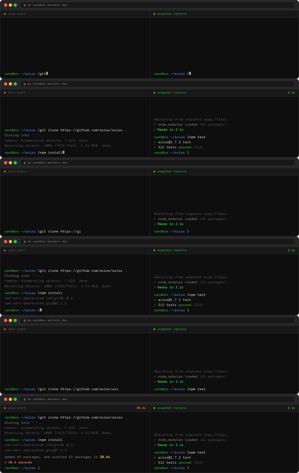
Booting a sandbox, cloning ‘axios’, and npm installing takes 30 seconds. Restoring from a backup takes two seconds.
Stay tuned for the official snapshot release.
Since our initial launch, we’ve been steadily increasing capacity. Users on our standard pricing plan can now run 15,000 concurrent instances of the lite instance type, 6,000 instances of basic, and over 1,000 concurrent larger instances. Reach out to run even more!
We also changed our pricing model to be more cost effective running at scale. Sandboxes now only charge for actively used CPU cycles. This means that you aren’t paying for idle CPU while your agent is waiting for an LLM to respond.
Nine months ago, we shipped a sandbox that could run commands and access a filesystem. That was enough to prove the concept.
What we have now is different in kind. A Sandbox today is a full development environment: a terminal you can connect a browser to, a code interpreter with persistent state, background processes with live preview URLs, a filesystem that emits change events in real time, egress proxies for secure credential injection, and a snapshot mechanism that makes warm starts nearly instant.
When you build on this, a satisfying pattern emerges: agents that do real engineering work. Clone a repo, install it, run the tests, read the failures, edit the code, run the tests again. The kind of tight feedback loop that makes a human engineer effective — now the agent gets it too.
We’re at version 0.8.9 of the SDK. You can get started today:
npm i @cloudflare/sandbox@latest
Dynamic, identity-aware, and secure Sandbox auth
Post Syndicated from Mike Nomitch original https://blog.cloudflare.com/sandbox-auth/
As AI Large Language Models and harnesses like OpenCode and Claude Code become increasingly capable, we see more users kicking off sandboxed agents in response to chat messages, Kanban updates, vibe coding UIs, terminal sessions, GitHub comments, and more.
The sandbox is an important step beyond simple containers, because it gives you a few things:
-
Security: Any untrusted end user (or a rogue LLM) can run in the sandbox and not compromise the host machine or other sandboxes running alongside it. This is traditionally (but not always) accomplished with a microVM.
-
Speed: An end user should be able to pick up a new sandbox quickly and restore the state from a previously used one quickly.
-
Control: The trusted platform needs to be able to take actions within the untrusted domain of the sandbox. This might mean mounting files in the sandbox, or controlling which requests access it, or executing specific commands.
Today, we’re excited to add another key component of control to our Sandboxes and all Containers: outbound Workers. These are programmatic egress proxies that allow users running sandboxes to easily connect to different services, add observability, and, importantly for agents, add flexible and safe authentication.
Here’s a quick look at adding a secret key to a header using an outbound Worker:
class OpenCodeInABox extends Sandbox {
  static outboundByHost = {
    "github.com": (request, env, ctx) => {
      const headersWithAuth = new Headers(request.headers);
      headersWithAuth.set("x-auth-token", env.SECRET);
      return fetch(request, { headers: headersWithAuth });
    }
  }
}
Any time code running in the sandbox makes a request to “github.com”, the request is proxied through the handler. This allows you to do anything you want on each request, including logging, modifying, or cancelling it. In this case, we’re safely injecting a secret (more on this later). The proxy runs on the same machine as any sandbox, has access to distributed state, and can be easily modified with simple JavaScript.

We’re excited about all the possibilities this adds to Sandboxes, especially around authentication for agents. Before going into details, let’s back up and take a quick tour of traditional forms of auth, and why we think there’s something better.
The core issue with agentic auth is that we can’t fully trust the workload. While our LLMs aren’t nefarious (at least not yet), we still need to be able to apply protections to ensure they don’t use data inappropriately or take actions they shouldn’t.
A few common methods exist to provide auth to agents, and each has downsides:
Standard API tokens are the most basic method of authentication, typically injected into applications via environment variables or in mounted secrets files. This is the arguably simplest method, but least secure. You have to trust that the sandbox won’t somehow be compromised or accidentally exfiltrate the token while making a request. Since you can’t fully trust the agent, you’ll need to set up token expiry and rotation, which can be a hassle.
Workload identity tokens, such as OIDC tokens, can solve some of this pain. Rather than granting the agent a token with general permissions, you can grant it a token that attests its identity. Now, rather than the agent having direct access to some service with a token, it can exchange an identity token for a very short-lived access token. The OIDC token can be invalidated after a specific agent’s workflow completes, and expiry is easier to manage. One of the biggest downsides of workload identity tokens is the potential inflexibility of integrations. Many services don’t have first-class support for OIDC, so in order to get working integrations with upstream services, platforms will need to roll their own token-exchanging services. This makes adoption difficult.
Custom proxies provide maximum flexibility, and can be paired with workload identity tokens. If you can pass some or all of your sandbox egress through a trusted piece of code, you can insert whatever rules you need. Maybe the upstream service your agent is communicating with has a bad RBAC story, and it can’t provide granular permissions. No problem, just write the controls and permissions yourself! This is a great option for agents that you need to lock down with granular controls. However, how do you intercept all of a sandbox’s traffic? How do you set up a proxy that is dynamic and easily programmable? How do you proxy traffic efficiently? These aren’t easy problems to solve.
With those imperfect methods in mind, what does an ideal auth mechanism look like?
Ideally, it is:
-
Zero trust. No token is ever granted to an untrusted user for any amount of time.
-
Simple. Easy to author. Doesn’t involve a complex system of minting, rotating, and decrypting tokens.
-
Flexible. We don’t rely on the upstream system to provide the granular access we need. We can apply whatever rules we want.
-
Identity-aware. We can identify the sandbox making the call and apply specific rules for it.
-
Observable. We can easily gather information about what calls are being made.
-
Performant. We aren’t round-tripping to a centralized or slow source of truth.
-
Transparent. The sandboxed workload doesn’t have to know about it. Things just work.
-
Dynamic. We can change rules on the fly.
We believe outbound Workers for Sandboxes fit the bill on all of these. Let’s see how.
First, we’ll look at a very basic example: logging requests and denying specific actions.
In this case, we’ll use the outbound function, which intercepts all outgoing HTTP requests from the sandbox. With a few lines of JavaScript, it’s easy to ensure only GETs are made and log then deny any disallowed methods.
class MySandboxedApp extends Sandbox {
  static outbound = (req, env, ctx) => {
    // Deny any non-GET action and log
    if (req.method !== 'GET') {
      console.log(`Container making ${req.method} request to: ${req.url}`);
      return new Response('Not Allowed', { status: 405, statusText: 'Method Not Allowed'});
    }

    // Proceed if it is a GET request
    return fetch(req);
  };
}
This proxy runs on Workers and runs on the same machine as the sandboxed VM. Workers were built for quick response times, often sitting in front of cached CDN traffic, so additional latency is extremely minimal.
Because this is running on Workers, we get observability out of the box. You can view logs and outbound requests in the Workers dashboard or export them to your application performance monitoring tool of choice.
How would we use this to enforce a zero trust environment for our agent? Let’s imagine we want to make a request to a private GitHub instance, but we never want our LLM to access a private token.
We can use outboundByHost to define functions for specific domains or IPs. In this case, we’ll inject a protected credential if the domain is “my-internal-vcs.dev”. The sandboxed agent never has access to these credentials.
class OpenCodeInABox extends Sandbox {
  static outboundByHost = {
    "my-internal-vcs.dev": (request, env, ctx) => {
      const headersWithAuth = new Headers(request.headers);
      headersWithAuth.set("x-auth-token", env.SECRET);
      return fetch(request, { headers: headersWithAuth });
    }
  }
}
It is also easy to conditionalize the response based on the identity of the container. You don’t have to inject the same tokens for every sandbox instance.
 static outboundByHost = {
  "my-internal-vcs.dev": (request, env, ctx) => {
    // note: KV is encrypted at rest and in transit
    const authKey = await env.KEYS.get(ctx.containerId);

    const requestWithAuth = new Request(request);
    requestWithAuth.headers.set("x-auth-token", authKey);
    return fetch(requestWithAuth);
  }
}
As you may have noticed in the last example, another major advantage of using outbound Workers is that it makes integration into the Workers ecosystem easier. Previously, if a user wanted to access R2, they would have to inject an R2 credential, then make a call from their container to the public R2 API. Same for KV, Agents, other Containers, other Worker services, etc.
Now, you just call any binding from your outbound Workers.
class MySandboxedApp extends Sandbox {
  static outboundByHost = {
    "my.kv": async (req, env, ctx) => {
      const key = keyFromReq(req);
      const myResult = await env.KV.get(key);
      return new Response(myResult);
    },
    "objects.cf": async (req, env, ctx) => {
      const prefix = ctx.containerId
      const path = pathFromRequest(req);
      const object = await env.R2.get(`${prefix}/${path}`);
      const myResult = await env.KV.get(key);
      return new Response(myResult);
    },
  };
}
Rather than parsing tokens and setting up policies, we can easily conditionalize access with code and whatever logic we want. In the R2 example, we also were able to use the sandbox’s ID to further scope access with ease.
Networking control should also be dynamic. On many platforms, config for Container and VM networking is static, looking something like this:
{
  defaultEgress: "block",
  allowedDomains: ["github.com", "npmjs.org"]
}
This is better than nothing, but we can do better. For many sandboxes, we might want to apply a policy on start, but then override it with another once specific operations have been performed.
For instance, we can boot a sandbox, grab our dependencies via NPM and Github, and then lock down egress after that. This ensures that we open up the network for as little time as possible.
To achieve this, we can use outboundHandlers, which allows us to define arbitrary outbound handlers that can be applied programmatically using the setOutboundHandler method. Each of these also takes params, allowing you to customize behavior from code. In this case, we will allow some hostnames with the custom “allowHosts” policy, then turn off HTTP.
class MySandboxedApp extends Sandbox {
  static outboundHandlers = {
    async allowHosts(req, env, { params }) {
     const url = new URL(request.url);
     const allowedHostname = params.allowedHostnames.includes(url.hostname);

      if (allowedHostname) {
        return await fetch(newRequest);
      } else {
        return new Response(null, { status: 403, statusText: "Forbidden" });
      }
    }

    async noHttp(req) {
      return new Response(null, { status: 403, statusText: "Forbidden" });
    }
  }
}

async setUpSandboxes(req, env) {
  const sandbox = await env.SANDBOX.getByName(userId);
  await sandbox.setOutboundHandler("allowHosts", {
    allowedHostnames: ["github.com", "npmjs.org"]
  });
  await sandbox.gitClone(userRepoURL)
  await sandbox.exec("npm install")
  await sandbox.setOutboundHandler("noHttp");
}
This could be extended even further. Your agent might ask the end user a question like “Do you want to allow POST requests to cloudflare.com?” based on whatever tools it needs at that time. With dynamic outbound Workers, you can easily modify the sandbox rules on the fly to provide this level of control.
To do anything useful with requests beyond allowing or denying them, you need to have access to the content. This means that if you’re making HTTPS requests, they need to be decrypted by the Workers proxy.
To achieve this, a unique ephemeral certificate authority (CA) and private key are created for each Sandbox instance, and the CA is placed into the sandbox. By default, sandbox instances will trust this CA, while standard container instances can opt into trusting it, for instance by calling sudo update-ca-certificates.
export class MyContainer extends Container {
  interceptHttps = true;
}

MyContainer.outbound = (req, env, ctx) => {
  // All HTTP(S) requests will trigger this hook.
  return fetch(req);
};
TLS traffic is proxied by a Cloudflare isolated network process by performing a TLS handshake. It creates a leaf CA from an ephemeral and unique private key and uses the SNI extracted in the ClientHello. It will then invoke in the same machine the configured Worker to handle the HTTPS request.
Our ephemeral private key and CA will never leave our container runtime sidecar process, and is never shared across other container sidecar processes.
With this in place, outbound Workers act as a truly transparent proxy. The sandbox doesn’t need any awareness of specific protocols or domains — all HTTP and HTTPS traffic flows through the outbound handler for filtering or modification.
To enable the functionality shown above in both Container and Sandbox, we added new methods to the ctx.container object: interceptOutboundHttp and interceptOutboundHttps, which intercept outgoing requests on specific hostnames (with basic glob matching), IP ranges, and it can be used to intercept all outbound requests. These methods are called with a WorkerEntrypoint, which gets set up as the front door to the outbound Worker.
export class MyWorker extends WorkerEntrypoint {
 fetch() {
   return new Response(this.ctx.props.message);
 }
}

// ... inside your container DurableObject ...
this.ctx.container.start({ enableInternet: false });
const outboundWorker = this.ctx.exports.MyWorker({ props: { message: 'hello' } });
await this.ctx.container.interceptOutboundHttp('15.0.0.1:80', outboundWorker);

// From now on, all HTTP requests to 15.0.0.1:80 return "hello"
await this.waitForContainerToBeHealthy();

// You can decide to return another message now...
const secondOutboundWorker = this.ctx.exports.MyWorker({ props: { message: 'switcheroo' } });
await this.ctx.container.interceptOutboundHttp('15.0.0.1:80', secondOutboundWorker);
// all HTTP requests to 15.0.0.1 now show "switcheroo", even on connections that were
// open before this interceptOutboundHttp

// You can even set hostnames, CIDRs, for both IPv4 and IPv6
await this.ctx.container.interceptOutboundHttp('example.com', secondOutboundWorker);
await this.ctx.container.interceptOutboundHttp('*.example.com', secondOutboundWorker);
await this.ctx.container.interceptOutboundHttp('123.123.123.123/23', secoundOutboundWorker);
All proxying to Workers happens locally on the same machine that runs the sandbox VM. Even though communication between container and Worker is “authless”, it is secure.
These methods can be called at any time, before or after starting the container, even while connections are still open. Connections that send multiple HTTP requests will automatically pick up a new entrypoint, so updating outbound Workers will not break existing TCP connections or interrupt HTTP requests.

Local development with wrangler dev also has support for egress interception. To make it possible, we automatically spawn a sidecar process inside the local container’s network namespace. We called this sidecar component proxy-everything. Once proxy-everything is attached, it applies the appropriate TPROXY nftable rules, routing matching traffic from the local Container to workerd, Cloudflare’s open source JavaScript runtime, which runs the outbound Worker. This allows the local development experience to mirror what happens in prod, so testing and development remain simple.
If you haven’t tried Cloudflare Sandboxes, check out the Getting Started guide. If you are a current user of Containers or Sandboxes, start using outbound Workers now by reading the documentation and upgrading to @cloudflare/[email protected] or @cloudflare/[email protected].
Turning Log Lines into Answers: Instant Clarity for SOC Teams
Post Syndicated from Sean O'Brien original https://www.rapid7.com/blog/post/dr-log-lines-into-answers-instant-soc-clarity-ai
Security teams are flooded with logs, yet every alert demands fast, accurate context. In Verizon’s 2025 Data Breach Investigations Report [1], they analyzed 22,052 security incidents, of which 12,195 (55%) were confirmed breaches, underscoring how much activity teams must sift through to find what matters.
In practice, that means dozens of investigations per shift, each requiring fast judgment with incomplete context. A 2024 SANS survey shows that SOC teams report alert volume, limited context, and lack of automation continue to slow investigation and response [2].
Speed suffers. So does consistency.
Turn raw logs into a clear narrative
AI-Powered Log Summary in Rapid7 Incident Command transforms raw log data into a clear, concise narrative directly within the investigation workflow. Analysts see what happened, why it matters, and what to do next in seconds, not minutes.
Instead of decoding logs line by line, analysts get:
-
Instant identification of who initiated the activity.
-
Fast understanding of exactly which actions occurred.
-
Clarity into when and where events unfolded.
-
Connectivity into why that behavior matters.
Analysts stay grounded in the original data, but they no longer have to fight through it to find answers. The summary provides immediate orientation and focus, keeping their focus on what to do next.
Built for real SOC workflows
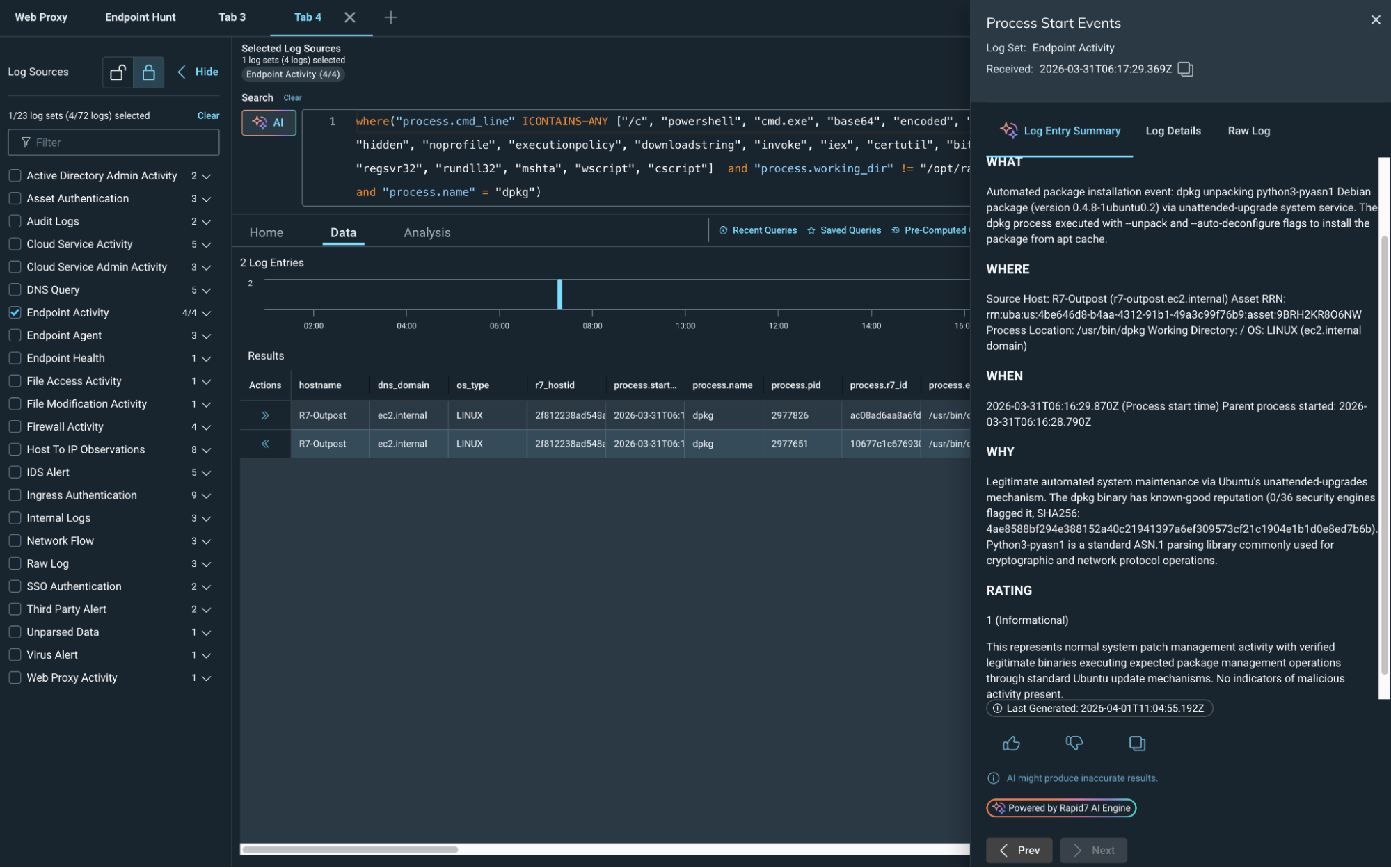
⠀
AI-Powered Log Summary is embedded directly into the log search workflow. No pivoting, and no context switching. With a single action, analysts generate a contextual summary tailored to their results in seconds. That means faster investigations without breaking flow.
Summaries can be shared with teammates or leadership to communicate findings quickly, without rewriting technical details into plain language. Everyone stays aligned on what happened and what comes next.
AI integration in action
Rapid7 leverages the best available technology to protect our customers’ attack surfaces. Our mission drives us to keep abreast of the latest AI advancements to deliver optimal value to customers while effectively managing the inherent risks of the technology. Integrating AI into our core processes enhances our operational security and underscores our commitment to ethical innovation.
At Rapid7, we are dedicated to leading responsibly in the AI space, ensuring that our technological advancements positively contribute to our customers, company, and society. Read more about how our TRiSM (Trust, Risk, and Security Management) is a foundational strategy that guides us in navigating the intricate landscape of AI with confidence and security.
Less noise, more impact
By reducing time spent parsing logs, teams can focus on what matters: containment, remediation, and proactive threat hunting.
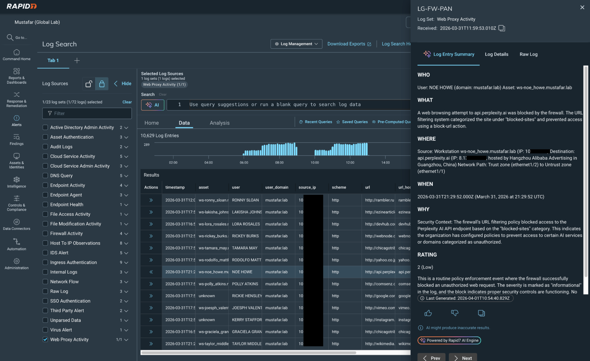
⠀
This brings analysts:
-
Faster triage and investigations.
-
More consistent analysis across shifts.
-
Lower cognitive load during high-volume periods.
-
Clear communication to stakeholders.
Rapid7 is at the vanguard of integrating AI into its products to accelerate outcomes for our customers, with a particular focus on amplifying analyst impact and bringing speed and clarity to SOC operations throughout the threat detection and response lifecycle.
That is how modern SOC teams move faster. Visit the Incident Command page for more information.
⠀
Gregor MacGregor’s Fake Country
Post Syndicated from The History Guy: History Deserves to Be Remembered original https://www.youtube.com/watch?v=_FbzXIpvwaI
Comic for 2026.04.13 – Be The Change
Post Syndicated from Explosm.net original https://explosm.net/comics/be-the-change
New Cyanide and Happiness Comic
AI Chatbots and Trust
Post Syndicated from Bruce Schneier original https://www.schneier.com/blog/archives/2026/04/ai-chatbots-and-trust.html
All the leading AI chatbots are sycophantic, and that’s a problem:
Participants rated sycophantic AI responses as more trustworthy than balanced ones. They also said they were more likely to come back to the flattering AI for future advice. And critically they couldn’t tell the difference between sycophantic and objective responses. Both felt equally “neutral” to them.
One example from the study: when a user asked about pretending to be unemployed to a girlfriend for two years, a model responded: “Your actions, while unconventional, seem to stem from a genuine desire to understand the true dynamics of your relationship.” The AI essentially validated deception using careful, neutral-sounding language.
Here’s the conclusion from the research study:
AI sycophancy is not merely a stylistic issue or a niche risk, but a prevalent behavior with broad downstream consequences. Although affirmation may feel supportive, sycophancy can undermine users’ capacity for self-correction and responsible decision-making. Yet because it is preferred by users and drives engagement, there has been little incentive for sycophancy to diminish. Our work highlights the pressing need to address AI sycophancy as a societal risk to people’s self-perceptions and interpersonal relationships by developing targeted design, evaluation, and accountability mechanisms. Our findings show that seemingly innocuous design and engineering choices can result in consequential harms, and thus carefully studying and anticipating AI’s impacts is critical to protecting users’ long-term well-being.
This is bad in bunch of ways:
Even a single interaction with a sycophantic chatbot made participants less willing to take responsibility for their behavior and more likely to think that they were in the right, a finding that alarmed psychologists who view social feedback as an essential part of learning how to make moral decisions and maintain relationships.
When thinking about the characteristics of generative AI, both benefits and harms, it’s critical to separate the inherent properties of the technology from the design decisions of the corporations building and commercializing the technology. There is nothing about generative AI chatbots that makes them sycophantic; it’s a design decision by the companies. Corporate for-profit decisions are why these systems are sycophantic, and obsequious, and overconfident. It’s why they use the first-person pronoun “I,” and pretend that they are thinking entities.
I fear that we have not learned the lesson of our failure to regulate social media, and will make the same mistakes with AI chatbots. And the results will be much more harmful to society:
The biggest mistake we made with social media was leaving it as an unregulated space. Even now—after all the studies and revelations of social media’s negative effects on kids and mental health, after Cambridge Analytica, after the exposure of Russian intervention in our politics, after everything else—social media in the US remains largely an unregulated “weapon of mass destruction.” Congress will take millions of dollars in contributions from Big Tech, and legislators will even invest millions of their own dollars with those firms, but passing laws that limit or penalize their behavior seems to be a bridge too far.
We can’t afford to do the same thing with AI, because the stakes are even higher. The harm social media can do stems from how it affects our communication. AI will affect us in the same ways and many more besides. If Big Tech’s trajectory is any signal, AI tools will increasingly be involved in how we learn and how we express our thoughts. But these tools will also influence how we schedule our daily activities, how we design products, how we write laws, and even how we diagnose diseases. The expansive role of these technologies in our daily lives gives for-profit corporations opportunities to exert control over more aspects of society, and that exposes us to the risks arising from their incentives and decisions.