Debian neither endorses nor prohibits the use of generative AI
tools in the development, maintenance, or documentation of
software, packaging, documentation, and other media published
within the Debian Project. We recognize that such tools can
substantially improve the productivity of contributors when used
responsibly, allowing volunteers to spend more of their limited
time on work that requires technical expertise, judgment, review,
and collaboration.
The Debian Project nevertheless expects that all contributions
submitted to Debian, regardless of how and with which tools they
were produced, satisfy the same standards of quality, correctness,
maintainability, and legal compliance. The use of a generative AI
tool does not diminish the contributor’s responsibility for the
work they submit. Contributors are expected to understand, review,
test, and, where appropriate, modify AI-assisted output before
incorporating it into Debian.
Today, git.kernel.org receives about 6M daily requests demanding to see
random commits. Of these, 66% are still immediately batted away with the Anubis
challenge, but 33% are now solving the math and getting through to the main site
— because apparently what we have to offer is worth spending a ton of cycles to
calculate the Anubis challenge.
It’s impossible to tell with certainty which of these are bots and which are
real humans — but chances are, if it’s asking for an old commit in a random old
fork, it’s probably not a real developer trying to do their work.
With a bunch of generous assumptions, legitimate requests are only about 2%
of git.kernel.org traffic — everything else are scrapers.
В първата част от материала описах какви са изискванията, причините да търся публичност на плановете за озеленяване, защо и как се предотвратява това. Във втората част дадох примери за проблеми с озеленяването при вече готови и пуснати в експлоатация сгради. Това беше възможно, защото Столична община разпозна надделяващия публичен интерес и предостави плановете.
В тази част ще дам още два примера на стоящи се в момента сгради. При тях виждам потенциал за проблеми предвид запечатания повърхностен слой, плитките лехи или пълната им липса, бетонните плочи на нивото на улицата без място за достатъчен почвен слой и други проблеми. В миналата статия споделих защо се спирам на тези четири примера, въпреки че нито инвеститорите, нито проектите са нещо специално що се отнася до строителството и проблемите в него в София и в цялата страна.
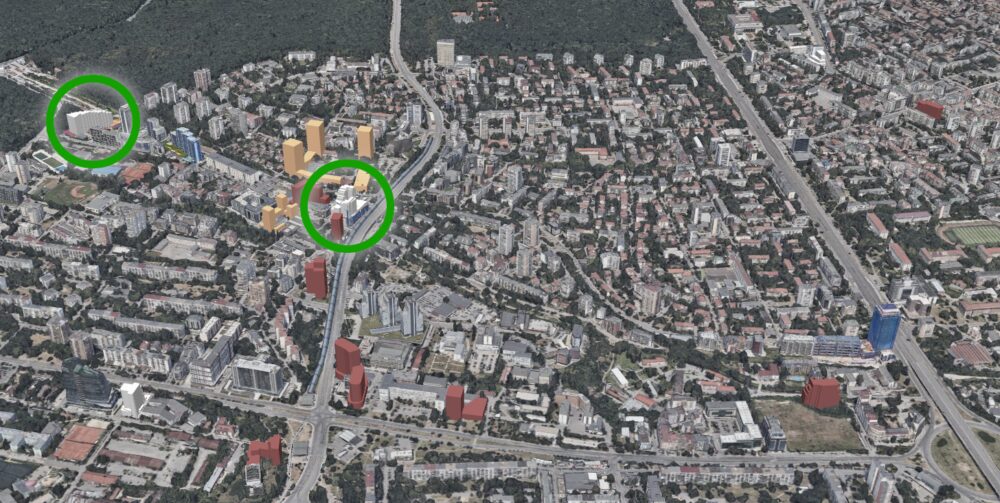
В тази част ще разгледаме строежите на Тинтява 80 и Диамант 3. Виждате ги отбелязани на картата. Накрая ще обсъдим защо това е важно и какво следва да се направи, за да се пресекат тези порочни практики. Както и в предишната част снимките в галериите се въртят автоматично. Може да ги спрете с бутона за пауза горе вдясно.
Тинтява 80
Разрешението за строеж е от 2019 г. и няколко пъти се променяше вътрешното устройство. След завършване на грубия строеж в края на 2023 г. или точно четири години след разрешението. В следващите над две години сградата беше изоставена и едва в началото на 2026-та беше подновена работа и името ѝ беше сменено на Twin Light.
Инвеститорът стана известен с друга негова сграда, която подобно на тази е отнела много време да се завърши, но точно преди пускане в експлоатация къса договорите и я препродава на значително по-високи цени. При тази сграда се е опитал друго – да индексира с до 100% платеното от купувачите. Доколкото става ясно от групите има множество дела срещу него, някои от които вече спечелени. Дали ще опита схемата с препродаването тук ще видим тепърва.
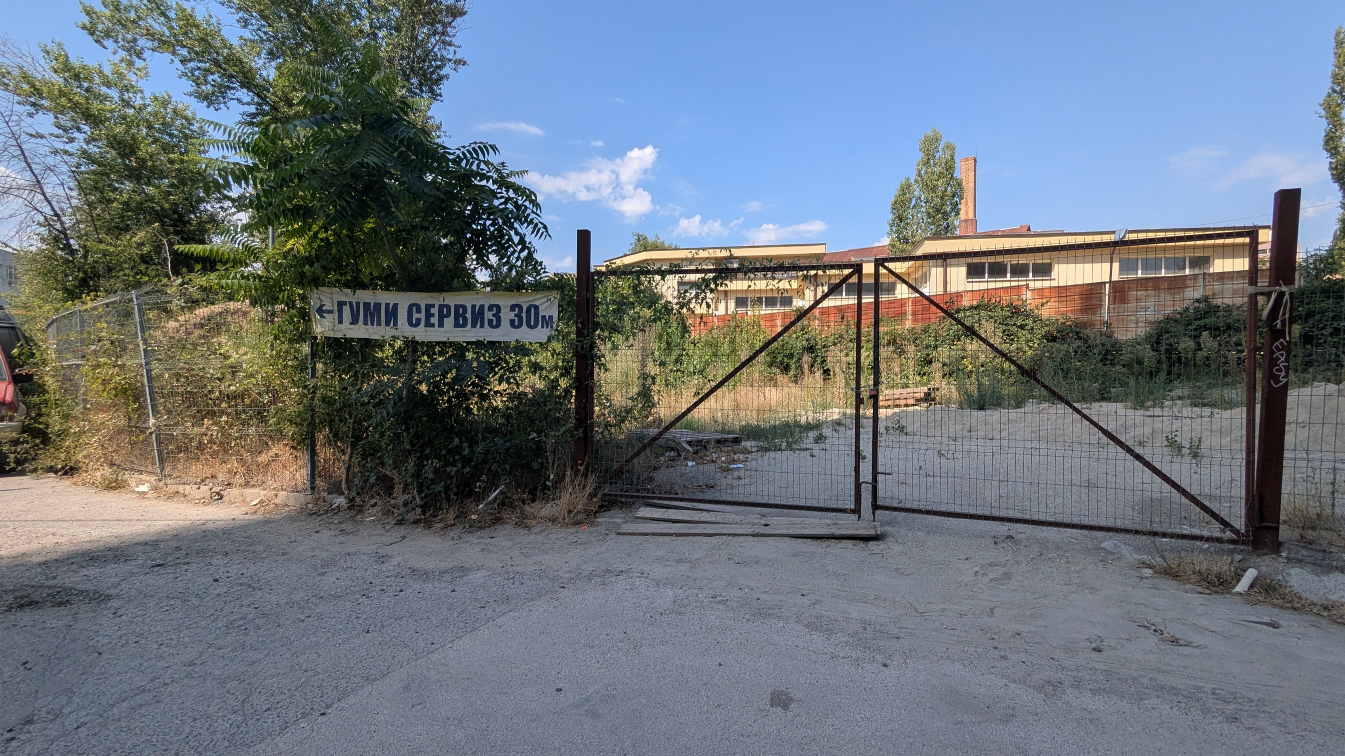
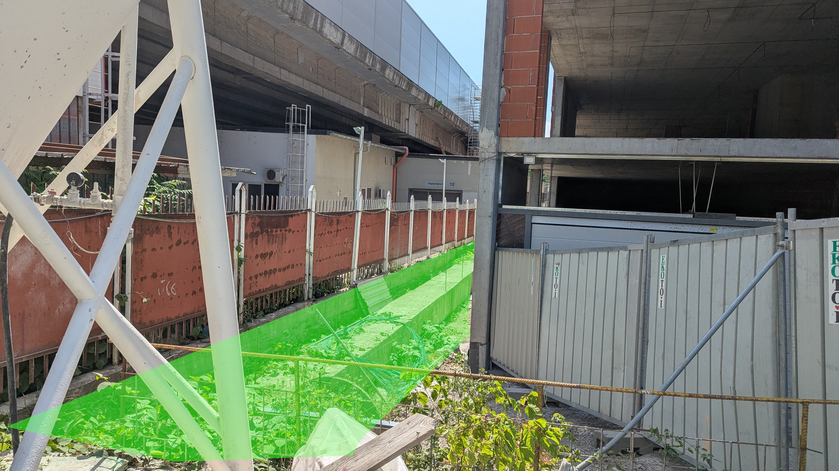
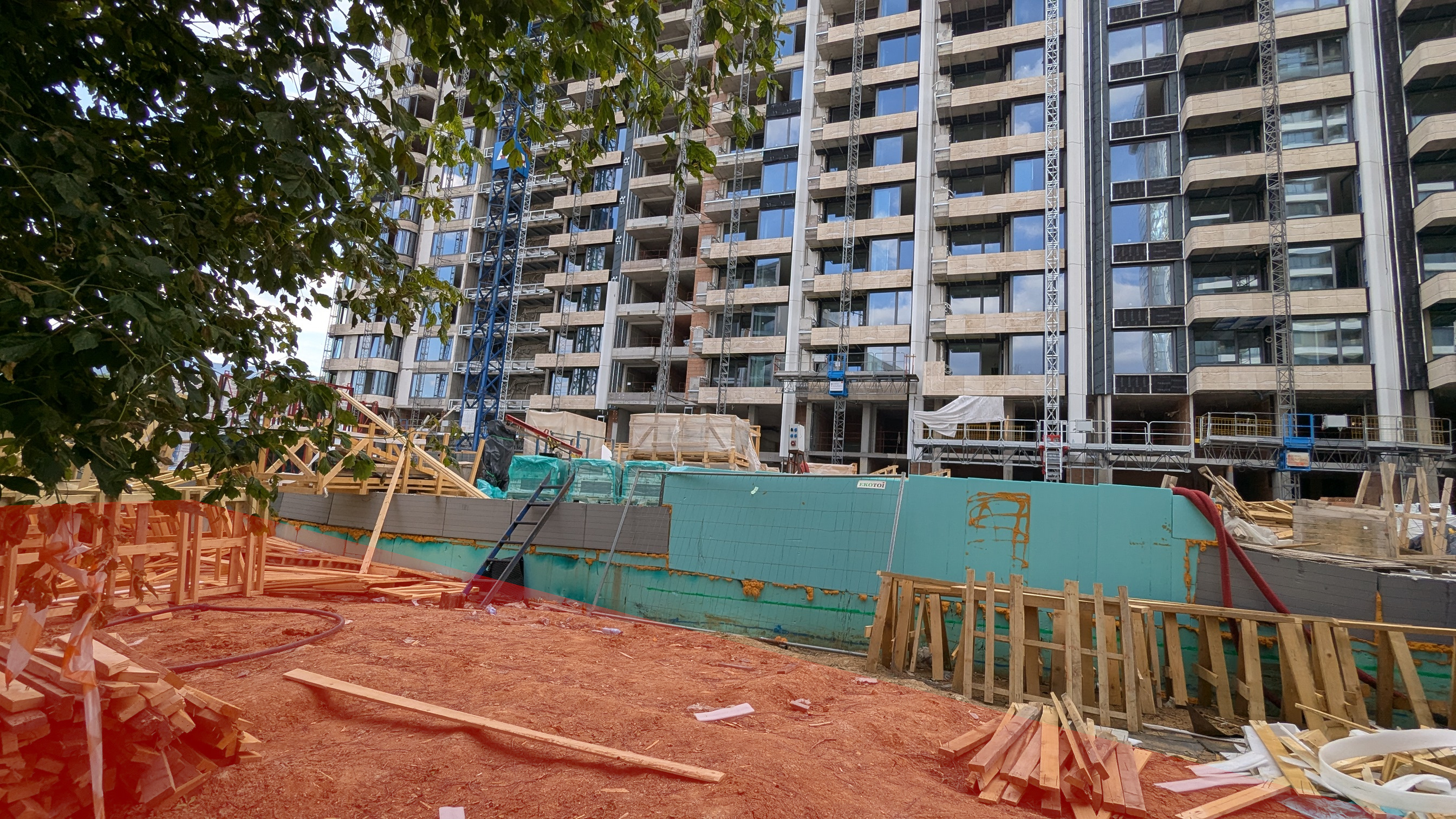
Междувременно имаше редица проблеми. Улицата беше разкопана без разрешение в почивен ден и оставена със зеещи дупки по думите на работниците, за да върже ТЕЦ и вода. Имот в близо собственост на държавата, а от скоро и на общината беше превърнато в сметище за строителни отпадъци и все още стои заградено (снимка 1). То също трябва да е част от Зеления ринг, макар да бяха изсечени всички дървета и почвеният слой беше изнесен, за да се заравни терена. От коментари на районната администрация става ясно, че е установено, че инвеститорът на тази сграда е виновен, но реални последствия нямаше.
В този контекст не следва да сме учудени, че срещаме проблемът и с изпълнението на самата сграда. За разлика от предишните две сгради, тази все още не е завършена. Това обаче ни позволя да видим какво е възможно, колко място са оставили за озеленяване и почвен слой. Проектът за озеленяване на имотът не беше много изчерпателен, но даде ключовите числа.
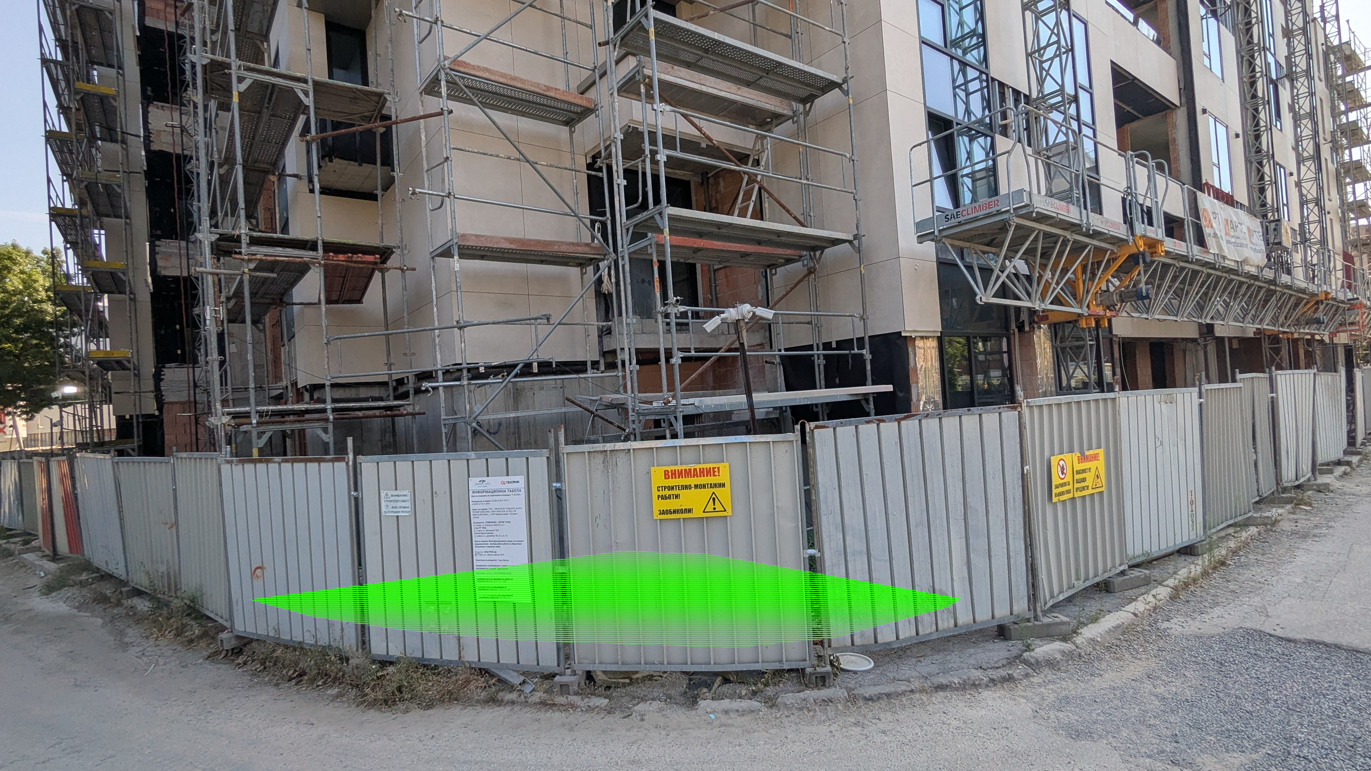
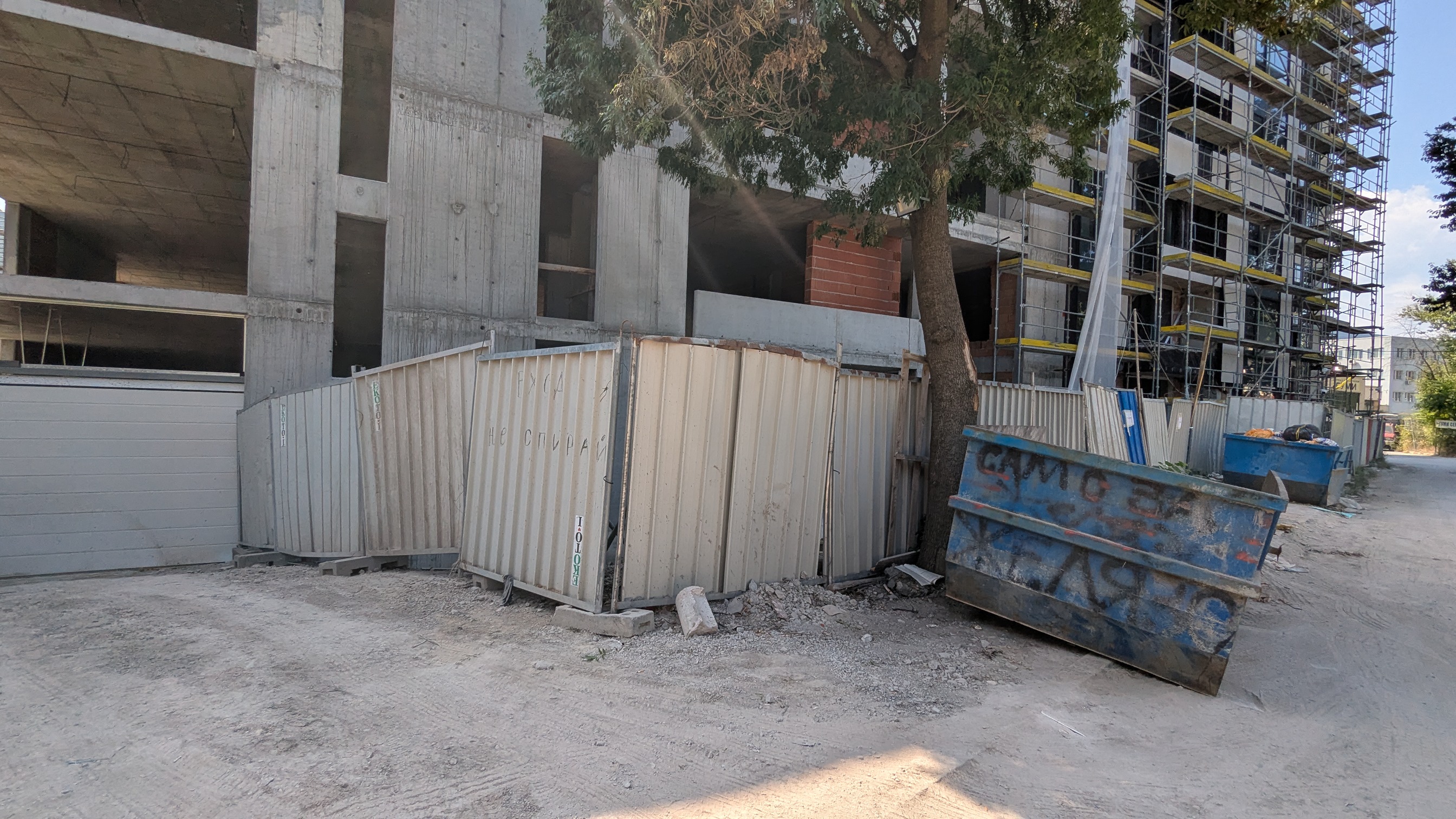
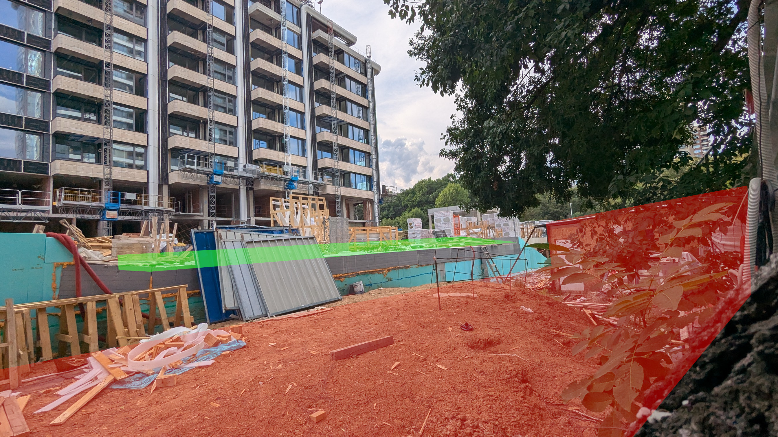
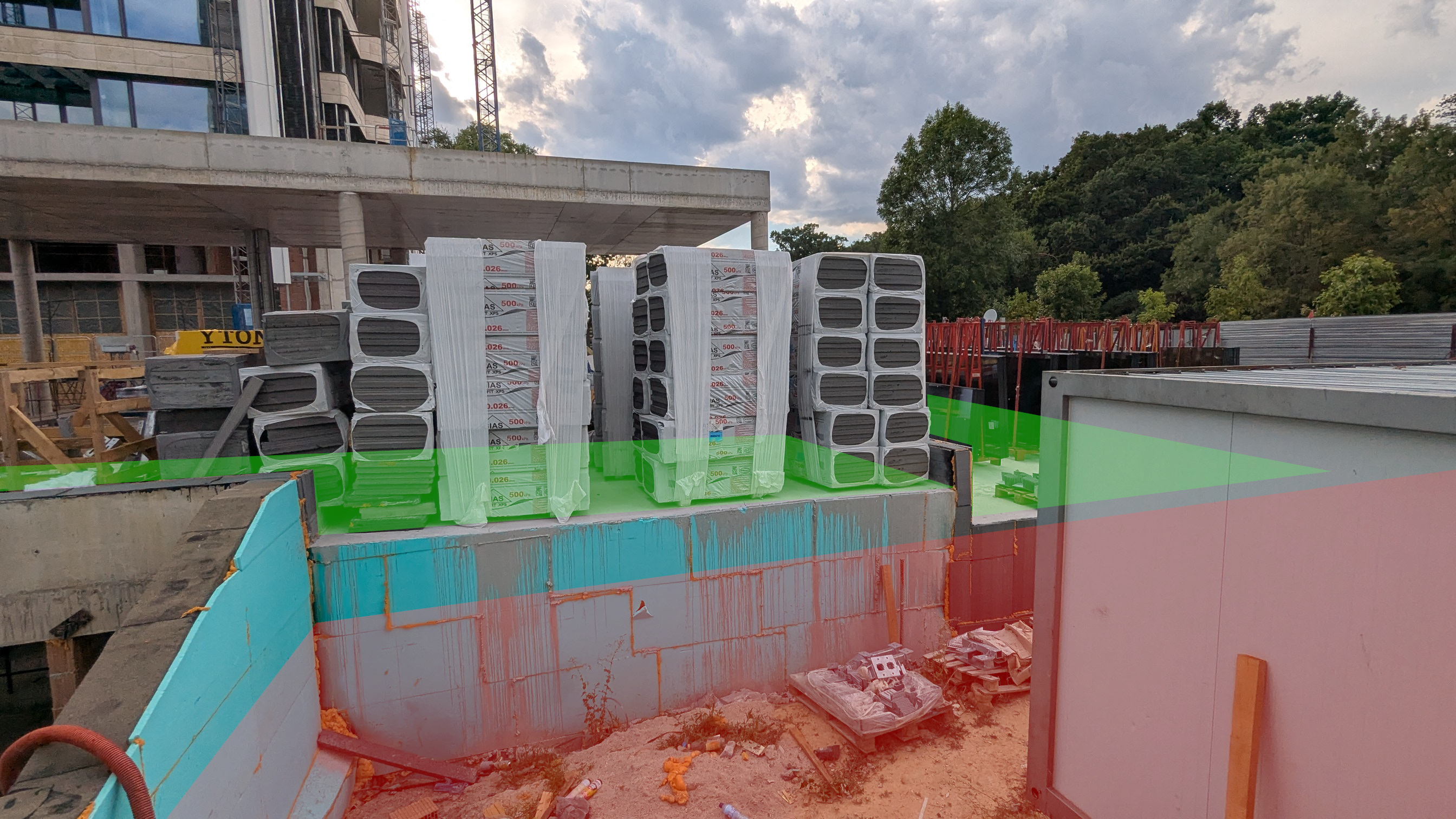
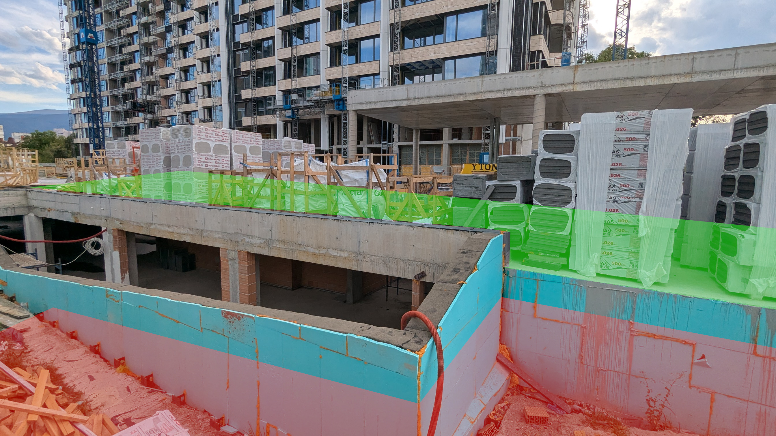
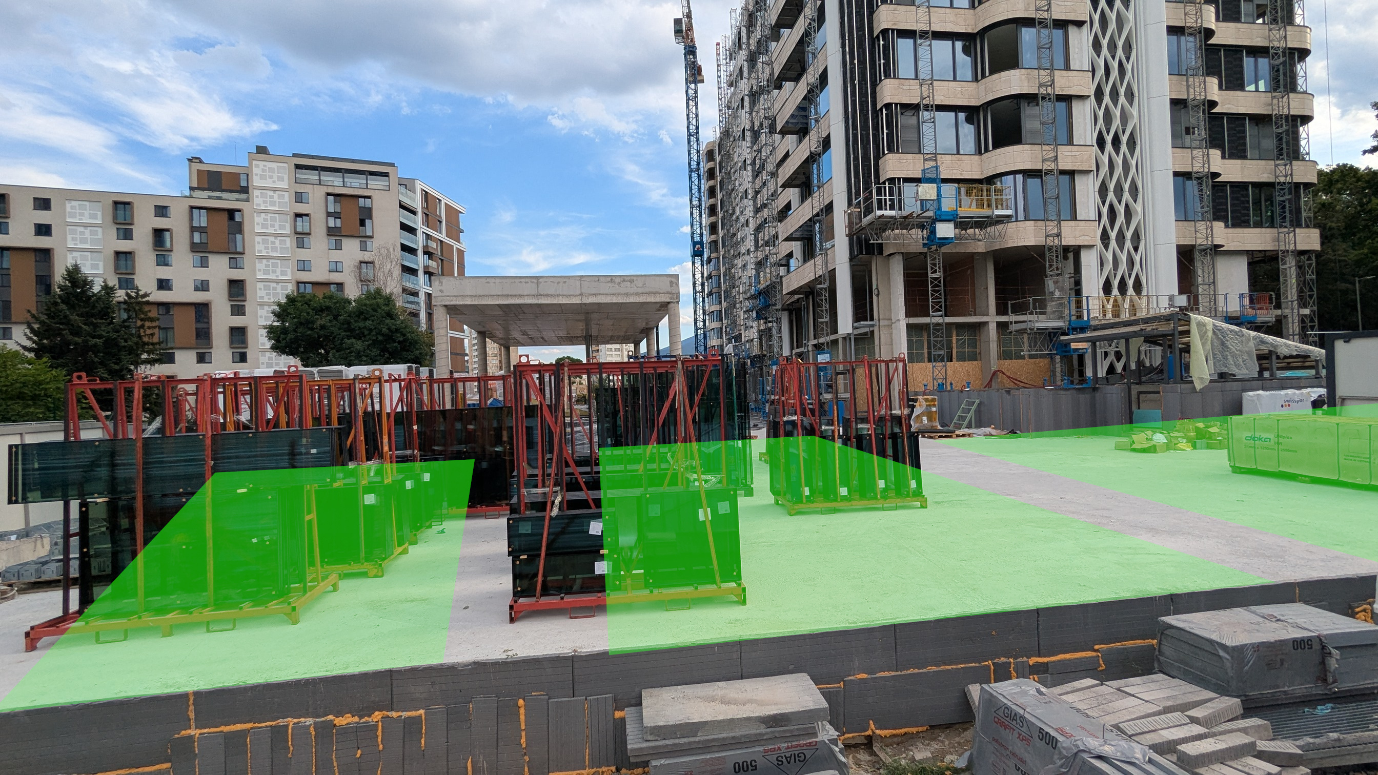
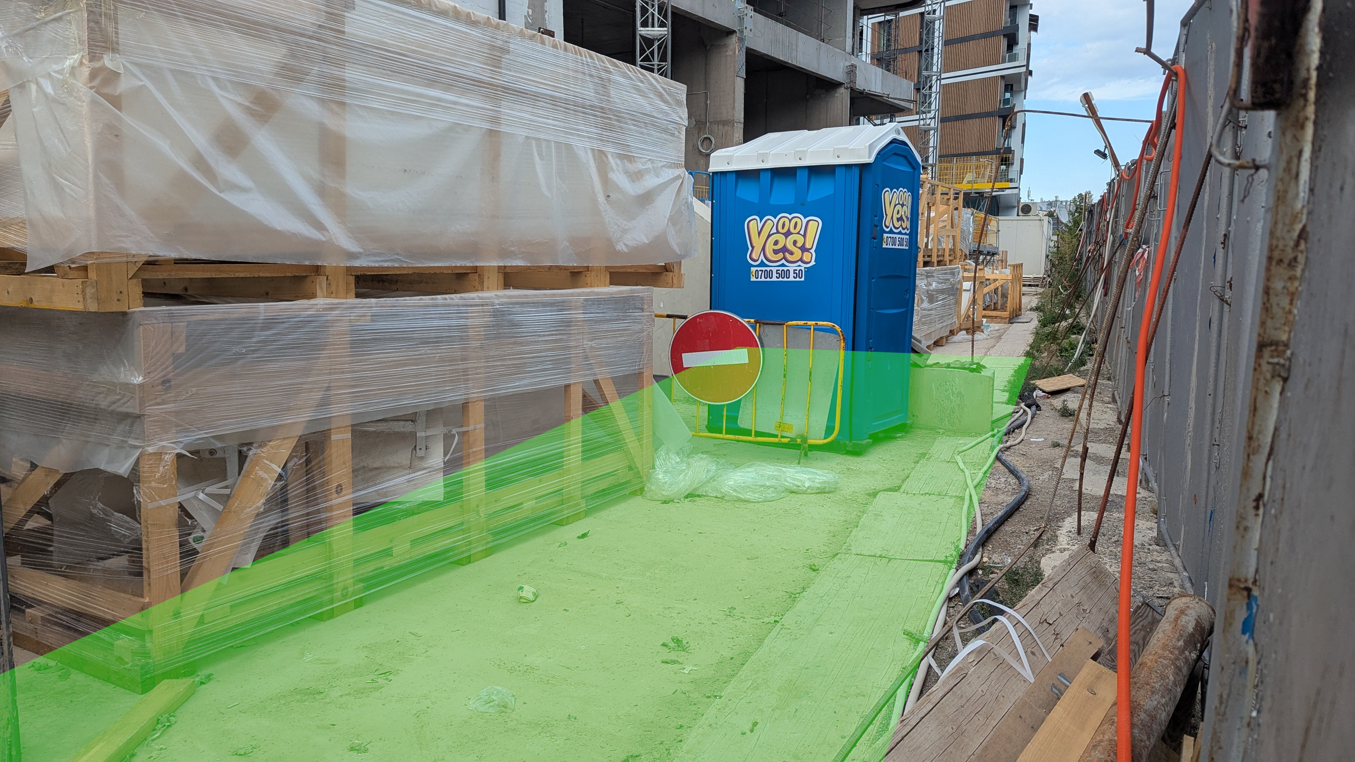
Сградата трябва да има 53 широколистни дървета, 22 иглолистни и 2277 храста. Предвижда 40.22% озеленена площ, 35% от нея да е висока дървесна растителност. От това озеленяване 10% ще са вертикално озеленяване по ограда като тук очаквам аналогични проблеми като предишната сграда – т.е. да ги няма. Плана за озеленяване предвижда, че 20% от него ще е върху естествен терен, т.е. няма да е върху бетонна плоча или гараж. Такива са терените отбелязани в зелено на снимки 2, 3, 5 7, 8 и 10. На място се вижда как те са бетонирани, както е целият парцел от край до край.
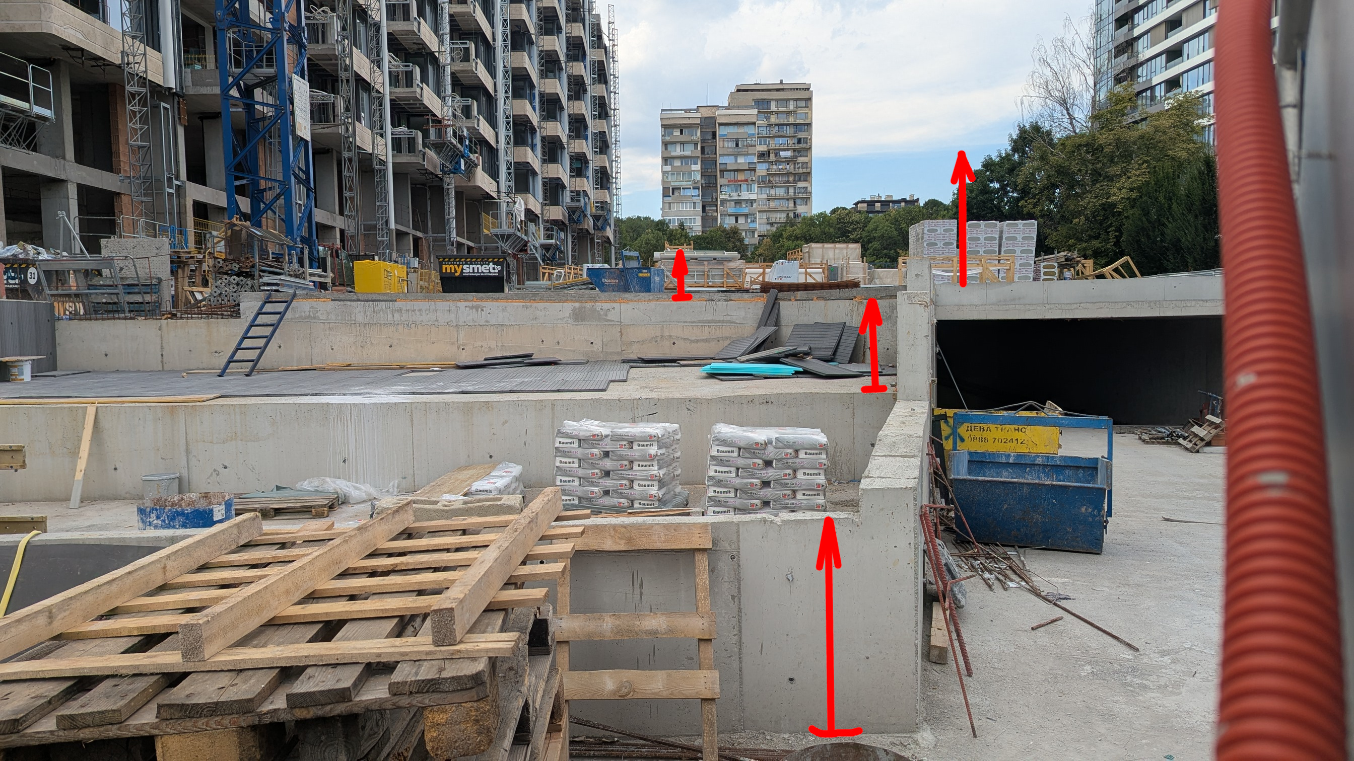
Аналогично в същия план е декларирано, че 52% от зелените площи ще са с дълбочина от над 120 см., което да позволи на дървета да оцелеят. Това е градината както във вътрешното пространство, така и задната част по източната ограда, която се вижда на снимка 9. На място и в двата случая се вижда, че бетонната плоча е не само плитка, а дори над нивото на улицата и не позволява добавяне описаният над метър почвен слой.
Общински имот заграден от години за сметище.
Планира се да има градинка и дърво в ъгъла.
Планирани за градинки по ръба на сградата.
Би следвало да има градинка с шест дървета между старото дърво и фасадата.
Тук по план е маркирано, че няма бетон, а естествена почва.
Тук е отбелязано, че няма бетон и ще има 21 дървета върху естествена почва
Тук е отбелязано, че няма бетон и ще има 21 дървета върху естествена почва
Тук е отбелязано, че няма бетон и ще има 21 дървета
Тук е отбелязано, че ще има 120 см почва и дръвета
Тук е отбелязано, че няма бетон, а естествена почва и място за градинка
Не знаем колко дървета ще има на имота, но на място вече се вижда, че планът одобрен от разрешението за строеж е невъзможен. На снимка 2 би трябвало да има високо широколистно дърво. За да оцелее и да отговаря на изискванията, освен, че трябва почвен слой, който плочата отдолу не позволява, трябва да има 3 метра от стената на сградата и още 2 метра до пътя. на място обаче се вижда, че вместо 5 метра разстояние има само 2.5 м., което е крайно недостатъчно и ако има дърво, то не може да се зачете към озеленяването и надали ще живее дълго.
Аналогично е положението при снимки 3, 4 и 5. Там не само трябва почвения слой да е естествен, т.е. да няма бетонна плоча отдолу, каквато се вижда ясно на снимките, но трябва да съберат общо 6 високи широколистни дървета. Там вече има дърво и според изискванията и измерените отстояния на място биха могли да съберат най-много две и то единствено, ако са точно пред планираните за витрини и вход на сградата. На тези места няма място оставено за адекватен почвен слой нито, за да може да оцелее дървото, нито да отговори на наредбата.
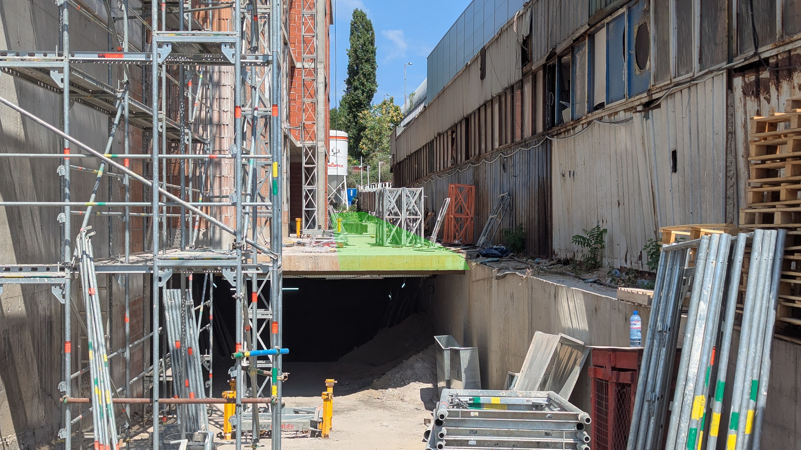
В снимки 6, 7, 8 и 9 се вижда отсечката от източната ограда. Там следва да посадят 21 високи широколистни дървета. Дори да успеят да ги сложат там отново отстоянията от сградата, оградата на съседния имот и моста на метрото не позволяват да се зачетат към коефициентът на висока дървесна растителност. Остава мистерия и как въобще е одобрен подобен план за озеленяване, който ще натика дърветата практически под моста на метрото. На снимките се вижда и бетонната стена на строежа, която не оставя място за корените на дърветата или почвен слой. Вероятно планират да сложат фиданки залепени до бетонната стена и да я скрият под 5 см. почва с малко трева както видяхме при Диамант 2. Разбира се, това би било в нарушение на наредбата и одобрения план, но при благожелателна приемателна комисия и особено членове там от районното кметство би им се разминало.
Не снимка 10 се вижда пространство, което би трябвало да е поне 50 квадрата зелена площ, поне една трета от което е с дълбочина от 120 см под нивото на улицата, а останалото – естествена почва без бетонни плочи под нея. Вижда се с просто око, че нито има толкова място за зеленина, нито вертикално е предвидено място за толкова почва.
Вътре в самия имот са описали 58 дървета в различни лехи. Там отново се вижда, че бетонът е на нивото на улицата и няма място за декларираните 120 см. почва. Вероятно ще поставят кашпи по подобие не East Plasa. Дори тогава обаче няма място за 58 дървета предвид изискванията за отстояние едно от други и 3 метра от сградата. Биха се побрали не повече от 40 дървета и то, ако няма никакви пътеки и други елементи и целият двор е само озеленяване.
Това, което видях в скиците ми показа, че не само ако се изпълни не би отговаряло на изискванията, но и предвид излятия вече бетон на нивото на улицата и по границите на имота е невъзможно да се осъществи по друг начин спазвайки минималните изисквания. В този смисъл сградата не би трябвало да получи акт 16 без сериозни нарушения от страна на ДНСК и районната администрация.
Диамант 3
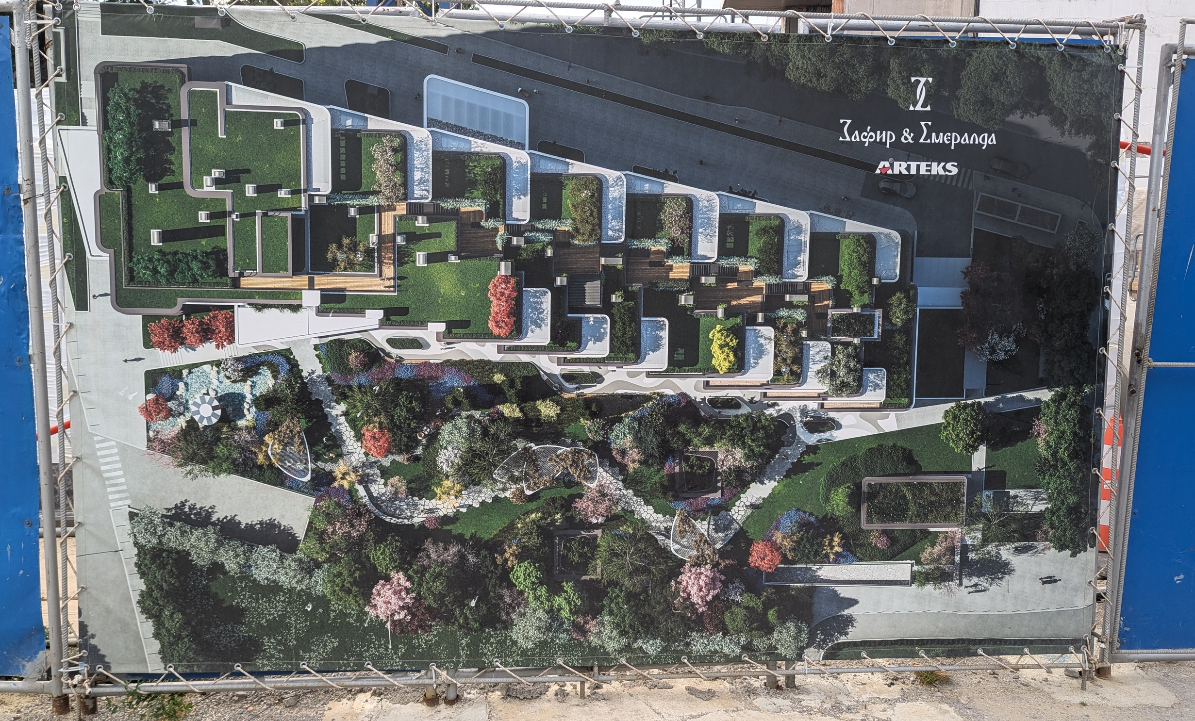
Официалното име на проекта е „Зафир и Емералда“, но всички го познават като Диамант 3 по обясними причини. Сградата се рекламира като „първата озеленена терасовидна сграда на Балканите“. На визуализациите виждате, че практически целият покрив е в трева (снимка 1) и поне между 10 и 20 дървета според коя картинка облепена по оградата гледате. В зимният вариант на визуализациите са сменили широколистните дървета с коледни елхи (снимка 2). Това може би предполага, че всички ще са на кашпи, които ще се сменят с кран или хеликоптер по два пъти в годината.
Разбира се, никой няма илюзии, че визуализаците имат нещо общо с реалността и затова имаме нужда от плановете за озеленяване. В тях изцяло липсва всякакво озеленяване по покрива. Няма причина да не го включат освен, ако нямат намерение да не го правят въобще. Също така, както се досещате, озеленяването в двоа няма да има нищо общо с картината на снимка 1.
В плана като неразделна част от строителните книжа и разрешителното за строеж са предвидени 64 широколистни дървета, 106 иглолистни дървета и храсти и 3221 цветя. С това и обещаните по скица зелени площи се надяват да достигнат 40% озеленяване, от които 36% са висока дървесна растителност.
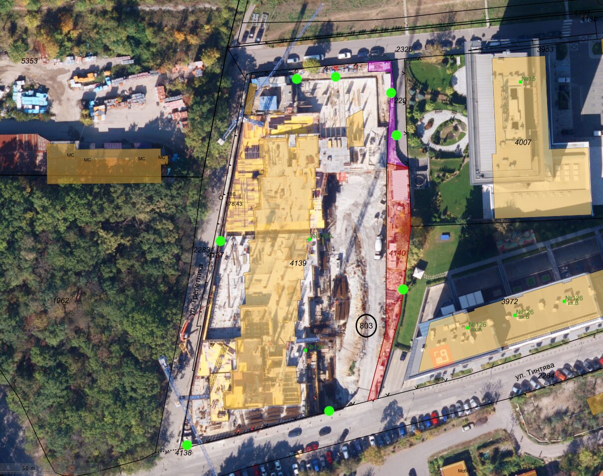
Нещо любопитно в този строеж са два парцела в съседство. Първият е 68134.803.4140 отбелязан с червено в снимка 3 и в началото си е с широчина едва три метра. Тогавашния главен архитект Здравков позволи той да се отдели от големия парцел с една единствена цел – да не позволи на съседните имоти да обжалват последвалите процедури и разрешение за строеж. Иначе е собственост на същия инвеститор. Впрочем, докато се е готвела тази схема, в интервю за Капитал споменах, че сградата ще има същите проблеми както другите им в карето с често спиране на тока. Тогава ми отговориха, че било лъжа и нямало спиране на тока в Диамант 1 и Диамант 2. Затова отговорих с данните от електроразпределителното дружество и други детайли. Над него има друг имот – 68134.803.1229. Той е държавна частна собственост и се използва за път за вход на гаража на Диамант 1. В лилаво е отбелязана обаче частта, която е в момента заградена от строежа. Очаквам подобно на общинският парцел да бъде приобщена към сградата и да си остане част от комплекса въпреки, че е държавна собственост.
Ключовото при тези два парцела е, че в тях няма разрешение за строеж и съответно всякакво озеленяване там не може да се брои към задължителното такова на Диамант 3. Аналогично на Диамант 2 обаче очаквам все пак да си ги препишат. В снимки 4 и 5 виждате в червено кое не се смята към строежа. Половината от червеното на снимка 7 е в държавния имот, а останалото червено в снимки 6 и 7 е предвидено за тротоар покрай входа на гаражите.
Визуализация представяща какво озеленяване обещават на купувачите.
Различна визуализация, в която дърветата по терасите са сменени с елхи.
Снимка на обекта от 2024 с наложени одобрената сграда и съседния държавен парцел.
Отбелязан е „буферен“ парцел невлизащ в разрешението за строеж.
Отбелязан е „буферен“ парцел невлизащ в разрешението за строеж.
Отбелязан е държавен имот, както и къде трябва да има озеленяване.
Отбелязан е държавен имот, както и къде трябва да има озеленяване.
Отбелязано къде трябва да има озеленяване с дървета.
Отбелязано къде трябва да има озеленяване с дървета.
Отбелязано къде трябва да има озеленяване с дървета.
Отбелязано къде трябва да има озеленяване.
Отбелязана е липса на дълбочина за почва според изискванията за дървета.
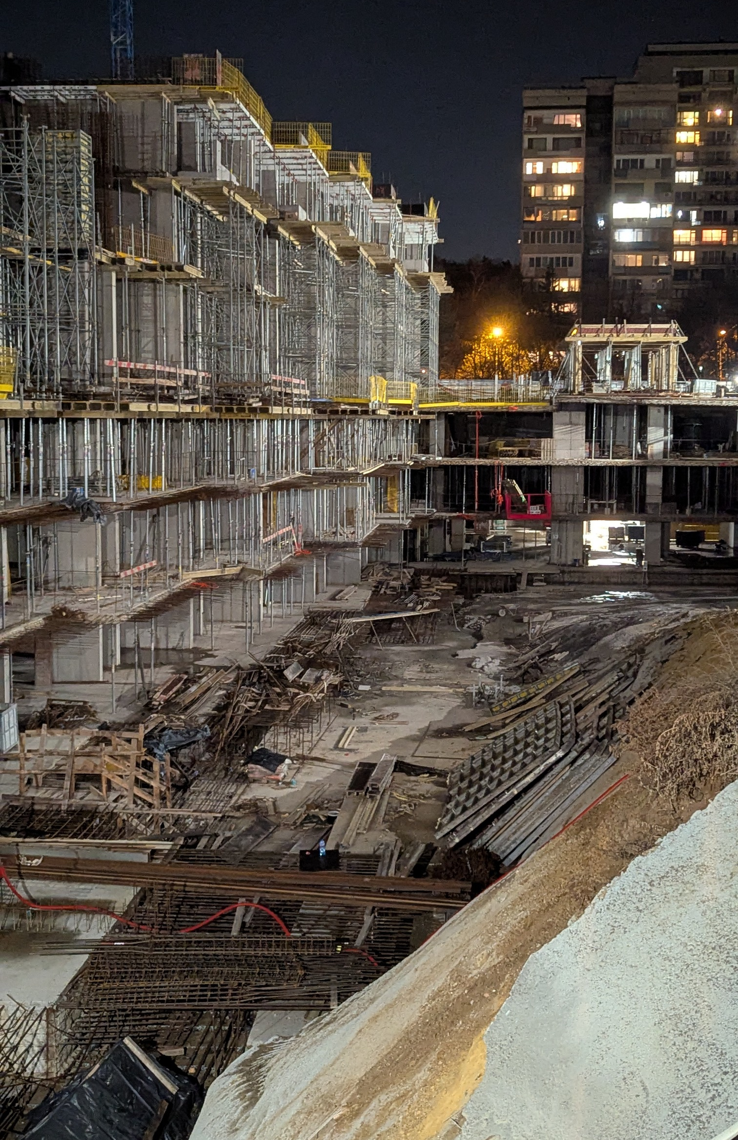
Снимка на подземните гаражи в строеж към 2025 г.
Зеленото в снимки 5 до 9 са предвидени за зелени площи с храсти и дървета според скицата на плана. Това задължава поне 30 см. почва за тревата, 60 см. за храстите и 120 см. за дърветата. На всички тях виждаме, че горната плоча на гаражите е на нивото на улицата и входовете на сградата. Това означава, че най-вероятно подобно на Диамант 2 ще пропуснат дърветата и ще сложа 5-10 см. бутафорна трева колкото за снимките. В същото време според плана за озеленяване там трябва да има поне 25 широколистни дървета и още 10 иглолистни. Същото важи и за снимка 10, където са предвидени поне 10 дървета в зоните отбелязани в зелено. Видимо това е невъзможно дори за изискванията за храсти.
Снимка 11 е от обратната страна на сградата, където е предвидена голяма зелена зона на ъгъла на Тинтява. Бетонът е на нивото на улицата и видимо няма място за почвен слой или храсти та ще е пак същото като Диамант 2. В снимка 12 виждаме нещо, което е обнадеждаващо, защото вече изглежда като издигнати лехи. Проблемът е, че са под метър във високата част, т.е. стават за храсти, но не и за дървета, които според плана за озеленяване трябва да са 7 там. На снимка 13 виждате изглед от подземните етажи във фаза на строежа към февруари 2025 г.
Друг съществен аспект от планът за озеленяването е отчетливата липса на резервоари за съхранение на дъждовна вода и системи за използването ѝ за напояване. Чл. 45, ал. 3 от наредбата влиза в сила на 27.07.2023, а разрешението за строеж на Диамант 3 е издадено на 2-ри ноември 2023 и влиза на 28-ми ноември. Това значи, че инвеститорът е длъжен да спази изискването. Разбира се, възможно е просто да не е отразена и да в предвидена в някоя част на подземията. Поради липсата на уточнение на за размера на резервоара, не бих се учудил инвеститорът да купи 70 л. варел за кисело зеле и да отбие номера също както с бутафорната трева. Само 30 евро ще излезе и с благожелателна приемателна комисия и особено членове там от районното кметство би им се разминало.
Какво от това?
Освен очевидното нехайство на отговорни институции в лицето на ДНСК и членовете на приемателната комисия, виждаме и системен отказ за извършваме на служебните задължения при сигнали за тези и други нарушения. Нещо повече, видяното от плановете за озеленяване на двата готови проекта показва, че проверки в миналото са били неправомерно затваряни и описаното в официални отговори в тях не отговаря на фактите.
Всичко това е възможно в немалка степен поради липсата на публичност на тези и други документи свързани с подобни мащабни проекти. Доколкото всеки има право да печели икономически от собствеността си – оставайки настрана придобиването на такава чрез корупция, измама или търговия на влияние във властта – има редица ограничения, с които всеки трябва да се съобразява. Целта на тези ограничения е да се запази безопасността на околните, публичната инфраструктура и интересите на съседите. Затова не би трябвало да се строи дискотека или казино до училище или в жилищен квартал като цяло. Затова има отстояния и безопасност както на използващите сградата, така и на околните. В огромната си част тези изисквания се заобикалят, но в някои случаи просто се пренебрегват.
Озеленяването може да не изглежда важно, но масовата му липса всъщност влошава здравето на всички чрез по-мръсния въздух и мръсотията, която се довлича след наводненията. Особено предполагаемата липса на резервоари за дъждовна вода в последния пример би показала нехайството за обществената безопасност, която инвеститорите имат. Вторият пример вече дава такива „резултати“, както е видно на снимките. В същото време всички се надпреварват да рекламират сградите си окъпани в зеленина с дървета никнещи от всяка стреха и канавка. Явно търсене за това има, но предлагането и най-вече изпълнението практически липсва.
Вторичен ефект от стриктното спазване на изискванията за озеленяване и основна причина да не се прави е, че се намалява печалбата от тези имоти. Тинтява 80 щеше да има поне едно от крилата по-малко. Хотелът на 4-ти км. щеше да е значително по-нисък и трудно щеше да направи схемата с чл. 27. Диамант 3 пък нямаше да може да продаде толкова паркоместа и навярно щеше да се наложи да направи сградата по-малка. Това не е угодно и цените на имотите в момента предразполагат към сериозен корекционен риск както за допускане на неправомерни планове, така и за бездействие при последващи проверки.
Разбира се, единствено циничността като типично българско качество ни води към предположението за описания риск. Не може да твърдим, че подобни практики е имало при който и да е от описаните тук и в предишната примери. За жалост, медийните статии в миналото за асансьори, едноименно лобистки поправки в закони, дела за укриване на данъци и некоректни търговски практики определено подплатяват значително тази циничност. Ако прочитът ми на документите е неправилен, което би било също разумно предположение, то не може да говорим дори за административно нарушение, с което се изчерпва личното ми мнение относно разминаването между видяното на място и плановете, до които ми беше даден достъп. При липсата на публичност на тези планове обаче трудно биха били прегледани от специалисти.
Всичко описано до тук показва нуждата от още прозрачност. Следва частите от строителните книжа като плановете за озеленяване, пожарна безопасност и транспортен анализ да са публични и свободно достъпни още на фаза инвестиционно намерение. Единният регистър към ЗУТ трябва да заработи и дори да се разшири с тези изисквания. Затова трябва законът за авторските права да се опрости позволявайки използването на тези части от архитектурни планове за нетърговски цели и лични цели изключвайки прилагането им в нови строежи. Така ще се защити интереса на архитекта като автор и в същото време ще позволи използването им от журналисти и жители на кварталите за обществен надзор.
Такъв надзор не би трябвало да бъде нужен. Положението не само в София, а и в цяла България е толкова плачевно, че дори при добро желание общините нямат достатъчно ресурс да проверяват всеки строеж. Затова не само се налага да се включва гражданското общество повече, но и трябват безкомпромисни мерки при нарушения. Включително разрушаване на части или цели сгради или задължение да се приведат според изискванията. Да, това ще засегне купувачите на имоти и ще се превърне в политически проблем абсолютно както виждаме в Баба Алино. Следва обаче да съдят инвеститорите за измама и некоректни практики и да се разбере най-накрая, че инвестицията в имоти е една от най-рисковите в България. Повече публични данни ще помагат на по-информиран избор в тази посока.
A tractor-trailer rollover sent a truckload of squid spilling into a Rhode Island roadway, leaving a stench as they sat in the road for hours in the summer heat. Local authorities have dubbed it the “Squidpocalypse of ’26.”
Méven Car has written a pair of interesting blog posts (part 1, part 2). The
first post is largely about some of the recent new features and performance work
that have gone into the Dolphin file
manager 26.08 release, as well as the KIO framework. The second looks at
the performance improvements and benchmarks for previous, current, and upcoming
releases.
Copying many small files is more than twice as fast as it was in April. The
gain falls off as files get larger, which is what you would expect: the fix is
to the per-file overhead, and once each file carries a megabyte of actual I/O
the overhead stops being what you are waiting for.
There is still a gap with cp, discussed at length in the
July post. KIO is doing more than cp does, but not five times more,
and the batching work that closes most of the rest of that gap is still in
progress.
Organizations in regulated industries such as financial services, government, defense, and healthcare restrict their sensitive workloads to isolated network environments with no access to the public internet. Until now, customers could restrict AWS Management Console access to authorized AWS accounts and corporate networks, but the console itself required internet connectivity. This was creating tension between operational convenience and network security controls.
We’re happy to announce that AWS Management Console Private Access is now generally available with support for virtual private clouds (VPCs) without internet connectivity. Organizations in regulated industries that restrict workloads to isolated network environments can now route all traffic for supported service consoles—including authentication flows, static assets (JavaScript, CSS, images), console-only APIs, and AWS service API calls—through AWS PrivateLink VPC endpoints, eliminating the need for an internet gateway, NAT gateway, or any route to the public internet. This capability is available in all AWS commercial Regions for a select set of supported service consoles.
In 2023, we launched AWS Management Console Private Access, which you can use to connect to the console by routing console, sign-in, and service API calls through VPC endpoints. However, accessing the console required internet connectivity for static assets and console-only APIs. This meant security teams faced a choice: allow internet connectivity to use the console or deny console access to operators working in network-isolated environments.
With this launch, AWS Management Console Private Access addresses two common scenarios:
Console traffic over internet restricted networks: Traffic for supported service consoles now flows entirely through your VPC endpoints—no proxy allowlists to maintain, no TLS-intercepting proxies to operate, and no CLI-only workflows to accept as a compromise. The same path works seamlessly from Amazon WorkSpaces, Amazon Elastic Compute Cloud (Amazon EC2) instances, and on-premises networks connected through AWS Direct Connect or AWS Site-to-Site VPN. Combined with sign-in resource control policies (RCPs) and sign-in resource policies, you can ensure that console authentication only succeeds from expected networks—even if valid credentials are presented elsewhere, the session is denied. Teams that previously relied on restricted egress rules or manual domain allowlists now get full console access with the same network controls they already trust.
Data-exfiltration prevention: Private Access enables you to restrict which AWS accounts and organizational identities can use the AWS Management Console from within your VPC. This prevents access from personal accounts and from accounts outside your organization. Attach a VPC endpoint policy with an aws:ResourceOrgID condition, and console actions are automatically scoped to resources inside your organization. Sign-in RCPs add a second layer by ensuring authentication only succeeds from networks within your perimeter. Together, these controls prevent supported service consoles from being used to access resources in accounts outside your organization—such as personal accounts—without requiring complex network-layer workarounds.
In this post, you will learn how AWS Management Console Private Access works in environments without internet connectivity, and how to layer access controls using VPC endpoint policies and sign-in resource control policies (RCPs) to strengthen your data perimeter.
Solution overview
AWS Management Console Private Access and sign-in resource control policies are a natural extension of the service control policies (SCPs), resource control policies, and VPC endpoint policies you already use for API traffic; now applied to the console session itself. The same data perimeter controls for identity, resource, and network that protect your programmatic access now protect interactive browser sessions too.
Perimeter
Control objective
Policy construct
Implementation Steps
Identity
Only trusted identities can access my resources
Sign-In RCPs and RBPs
Restrict which principals can sign in to the console. Before authentication, signin:PrincipalArn is available for exemptions only. After authentication, RCPs restrict at the organization, account, or principal level (aws:PrincipalOrgID, aws:PrincipalAccount, aws:PrincipalArn); RBPs restrict at the account or principal level.
Identity
Only trusted identities are allowed from my network
Console VPC endpoint policy and Sign-In VPC endpoint policy
Console endpoint: aws:PrincipalOrgID or aws:PrincipalAccount on signed-in identities. Sign-In endpoint: aws:ResourceOrgID or aws:ResourceAccount before authentication, principal and resource keys after authentication. Blocks sign-in to accounts outside your organization, such as personal accounts, from your network.
Resource
My identities can access only trusted resources
SCP
Resource perimeter SCP with aws:ResourceOrgID follows your principals into every console session; each service API call the console makes on their behalf is denied if the target resource is outside your organization.
Resource
Only trusted resources can be accessed from my network
Console VPC endpoint policy and service VPC endpoint policies
Console endpoint policy with aws:ResourceOrgID and aws:ResourceAccount scopes what the console can reach through your network.
Network
My identities can access resources only from expected networks
SCP
Network perimeter SCPs that use aws:SourceVpc deny your principals’ service calls from outside expected networks. With Private Access, requests proxied by the console to supported services carry aws:SourceVpc set to the VPC hosting your Private Access endpoints. Direct browser requests carry VPC context only when the service has its own VPC endpoint, so configure endpoints for every service you use. AWS recommends conditioning on aws:SourceVpc rather than specific aws:SourceVpce values.
Network
My resources can only be accessed from expected networks
Sign-In RBPs and RCPs and network perimeter RCPs
Sign-In policies deny console authentication from unexpected networks using aws:SourceIp, aws:SourceVpc, aws:SourceVpce, and aws:VpcSourceIp in both pre-authentication and post-authentication statements. Network perimeter RCPs apply the same network conditions to your data resources for any access path.
With this launch, Console Private Access routes browser traffic for supported service consoles through VPC endpoints, including:
Authentication flows – Sign-in, credential exchange, and session token requests
Static assets – JavaScript, CSS, and images that render the console UI
Service console API calls – The backend requests made when users interact with service consoles
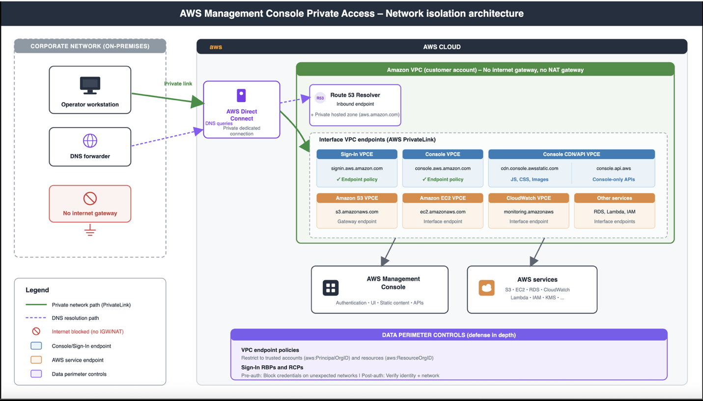
How traffic flows from a workload in a private VPC through the three Private Access endpoints, with no path to the public internet (shown in Figure 1):
The operator’s browser requests <region>.console.aws.amazon.com.
The corporate DNS forwarder forwards the query to an Amazon Route 53 Resolver inbound endpoint configured within the VPC, which forwards the traffic to the console VPC endpoint.
Browser traffic flows from on-premises through Direct Connect (or AWS Site-to-Site VPN) to the VPC, and the VPC endpoint routes traffic to the console service over the AWS private network.
The console service redirects to the SignIn endpoint <region>.signin.aws.amazon.com to establish a browser session.
The DNS now resolves to the SignIn VPC endpoint’s private IP addresses, and browser traffic flows to the SignIn service over the AWS private network.
After entering credentials, the SignIn service evaluates VPC endpoint policies, in addition to resource-based policies (RBPs) and RCPs, then redirects back to the console.
The console evaluates VPC endpoint policies, loads static content from the console API VPC endpoint, and enforces identity and resource restrictions when making calls to AWS service APIs.
Users can now access the AWS Management Console over Private Access.
Figure 1: Network isolation architecture
Deploy a pilot of AWS Management Console Private Access
This high-level walkthrough sets up AWS Management Console Private Access for a single AWS Region within one organizational unit (OU). We recommend rolling out incrementally; validate each step before you expand to additional Regions and OUs.
If you want to validate the mechanics of a Private Access deployment before you build out the full solution, the Getting started with a test environment guide walks you through a minimal configuration: a single VPC with the three Private Access endpoints and a permissive policy. This gives you a working setup to experiment with, independent of the deployment described in the rest of this post. To understand how sign-in policies can verify a user’s network location when they access the console, see Controlling console access with resource-based policies and resource control policies.
Prerequisites
You must have the following prerequisites:
An AWS account that’s a member of an organization within AWS Organizations. The example RCP in Step 4 requires the management account access.
Before changing anything, use CloudTrail to map how your users access the console today. Search for eventName = ConsoleLogin over a representative window (we recommend 30 days) and review the sourceIPAddress, vpcEndpointId, and awsRegion fields. Identify which identity types are in use: root user, IAM user, SAML federation, and AWS IAM Identity Center. Decide which OU or account you will pilot with.
Note: A misconfigured sign-in policy can lock users out of the console. Avoid piloting in a production or shared account. Instead, use a dedicated test account and configure a break-glass principal (covered in Step 5) before enabling access enforcement.
Step 2: Create the Private Access VPC endpoints
In your chosen Region, create or identify a VPC to host the endpoints, then create three interface VPC endpoints in that VPC:
com.amazonaws.<region>.console for the console.
com.amazonaws.<region>.signin for AWS Sign-In.
com.amazonaws.<region>.console-static for console-only APIs. This endpoint is required only if your VPC has no internet path.
Step 3: Configure private DNS for AWS Management Console Private Access
To use AWS Management Console Private Access, you must configure private DNS so that the console domains—.console.aws.amazon.com, .signin.aws.amazon.com, and the associated static-content domains—resolve to your interface endpoints’ network interfaces within your VPC.
For workloads inside your VPC: If the workloads in your VPC use the default Amazon Route 53 Resolver, no additional DNS configuration is required. When you create each interface endpoint, enable the private DNS name option (set PrivateDnsEnabled = true). The public console domains will then resolve automatically to the endpoint network interfaces inside your VPC. If you use a custom DNS resolver or a private hosted zone, you must configure it explicitly to map the console domains to the endpoint addresses. See Working with private hosted zones for more information. For the complete list of domains and detailed DNS configuration steps, see the AWS Management Console Private Access required endpoints documentation.
For workloads outside your VPC: For workloads that reach the endpoints from outside the VPC—such as corporate offices connecting over AWS Direct Connect or AWS Site-to-Site VPN—ensure that your corporate DNS resolver returns the endpoint addresses for these domains. See Simplify DNS management in a multi-account environment with Route 53 Resolver for more information.
Step 4: Verify private connectivity
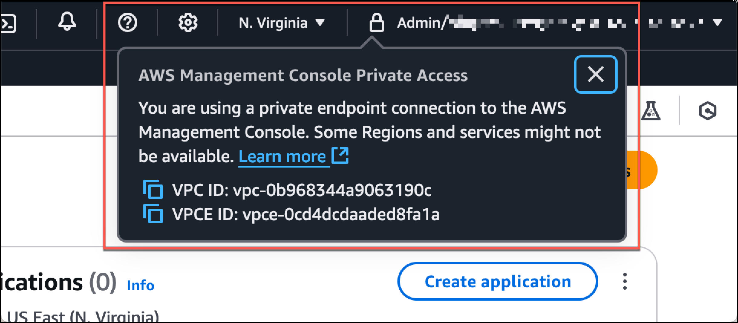
Sign in to the console from a workload inside your VPC. The console should load normally. To confirm that traffic is routing through your VPC endpoints, look for the lock icon in the console navigation bar, shown in Figure 2.
Figure 2: Console Private Access
You can also verify in CloudTrail that recent ConsoleLogin events show the vpcEndpointId field populated with one of your endpoint IDs. Here’s an example CloudTrail ConsoleLogin event snippet showing the vpcEndpointId field:
If the AWS Management Console doesn’t load, work through the following checks.
Private DNS is enabled on each interface endpoint (or your custom resolver returns the endpoint addresses)
When Private DNS is enabled, AWS automatically creates the DNS entries that resolve the service domains (such as console.aws.amazon.com) to the private IP addresses of your VPC endpoints. Without it, your browser still routes to the public AWS endpoints, bypassing your private access setup entirely.
Confirm that each endpoint shows PrivateDnsEnabled:
Then, from within your VPC, verify that the domains resolve to private addresses:
nslookup console.aws.amazon.com
nslookup signin.aws.amazon.com

# Should return a private IP (e.g., 10.x.x.x), not a public one
Each query should return a private IP address from your VPC CIDR range. If you use a custom DNS resolver instead of the Amazon-provided DNS, ensure your forwarding rules direct the AWS domain queries to the Route 53 Resolver inbound endpoints in your VPC.
The endpoint security groups allow HTTPS (TCP 443) from your workload subnets
Each VPC endpoint creates elastic network interfaces (ENIs) in your subnets, and these ENIs are governed by security groups. If those security groups don’t permit inbound HTTPS traffic from your workloads, the connection fails silently.
Identify the security groups attached to your endpoints:
aws ec2 describe-vpc-endpoints --vpc-endpoint-ids vpce-0abc123def456789a \
  --query "VpcEndpoints[].Groups[].GroupId" --output text
Then verify that each security group allows inbound TCP 443 from your workload subnets:
For traffic from outside the VPC (Direct Connect or Site-to-Site VPN), corporate DNS returns the endpoint IPs and the route propagates correctly
If you access the console from an on-premises workstation connected over AWS Direct Connect or AWS Site-to-Site VPN, two additional conditions must be met.
Your corporate DNS must resolve the AWS domains to the VPC endpoint private IPs. From your on-premises machine, run:
nslookup console.aws.amazon.com
If this returns public AWS IPs, your corporate DNS isn’t forwarding queries through Route 53 Resolver. Configure conditional forwarding for the aws.amazon.com and amazonaws.com domains to your Resolver inbound endpoint IPs.
Second, network routes must propagate correctly. Ensure the route table associated with your endpoint subnets has propagated routes from your virtual private gateway (VGW) or transit gateway, so return traffic can reach your on-premises network. Verify this with:
A quick end-to-end validation: Run traceroute console.aws.amazon.com from your workstation and confirm the path uses private hops only—no traffic should traverse the public internet.
If the console loads but the lock icon is missing
If the console loads but the connection isn’t private (for example, the lock icon is missing), the browser is reaching the console over the public internet instead of through your VPC endpoints.
Run nslookup console.aws.amazon.com from a workload inside the VPC. The result should be a private IP from your VPC CIDR range. A public IP means DNS is bypassing the endpoint, which usually happens because Private DNS has not been enabled on the interface endpoint (set PrivateDnsEnabled = true).
For workloads outside the VPC, make sure your corporate DNS forwards the console domains into the VPC, for example, through an Amazon Route 53 Resolver inbound endpoint.
Step 5: Apply VPC endpoint policies
Attach an endpoint policy to the console and AWS Sign-In endpoints that limits access to identities in your organization. The static-content endpoint doesn’t support endpoint policies.
Begin with a permissive Allow * policy and confirm that traffic routes through the endpoints (you should see the vpcEndpointId field populated in CloudTrail console events). After confirming the routing, add restrictions to your VPC endpoint policy and observe the traffic.
A starter policy uses two condition keys: aws:PrincipalOrgID to restrict identities to your organization and aws:ResourceOrgID to restrict the resources the console can reach to your organization’s resources. The full reference, including additional condition keys and resource-restriction patterns, is in the AWS Management Console Private Access user guide.
Sign-In policies deny console authentication requests that don’t match your network or principal conditions. The policy is composed of a pre-authentication statement covering signin:Authenticate and a post-authentication statement covering signin:AuthorizeOAuth2Access and signin:CreateOAuth2Token. Include both statements.
For your pilot, deploy the policy as an RCP from your AWS Organizations management account. When enabled, the RCP applies to all accounts in your organization, so we recommend piloting in a dedicated test organization before rolling it out broadly. Activate enforcement by calling the signin:PutConsoleAuthorizationConfiguration API for the organization in the us-east-1 Region (AWS Sign-In replicates policies globally from there). Resource permission statements have no effect until console authorization is enabled.
Important: Configure at least one excluded principal as a break-glass path before you enable the RCP. The recommended principal is a dedicated IAM role.
Write the permission statements that define the network conditions: Example – Restrict access to corporate VPC:
So far, the console shell loads, the lock icon appears, and your Sign-In policy lets approved identities through. If you sign in to a service console such as the AWS Key Management Service (AWS KMS) console, the page might fail to load resources or hang. The Private Access endpoints carry the console shell, not the service API calls that the console makes on your behalf. In a VPC without an internet gateway, those calls have nowhere to go.
Add a VPC endpoint for the service itself. For the pilot, create an AWS KMS interface endpoint (com.amazonaws.<region>.kms) in the same VPC, with Private DNS enabled. Open the AWS KMS console from inside the VPC and confirm the list of keys loads. Repeat for each service your users need on day one. Please note that a single service console often calls more than one AWS service API. If a console loads but parts of the page show errors or stay empty, the most common cause is a missing endpoint for one of the services it depends on.
The current list of services that support PrivateLink is in the AWS PrivateLink documentation. Service consoles whose services don’t support PrivateLink will not work in a no-internet VPC and need to be handled separately.
Step 8: Hide Regions and services you haven’t configured (optional)
Console links to a service or Region that you don’t have endpoints for will fail inside your VPC. To prevent users from navigating to broken pages, use User Experience Customization (UXC) to hide Regions and services that aren’t part of your Private Access deployment. UXC is configured at the account level and applies to navigation, search results, and service-selection drop-downs.
Step 9: Validate, then expand
After applying the endpoint policies and the Sign-In RCP to one pilot account:
Sign in from inside the corporate network. The session should succeed.
Sign in from outside the corporate network. The session should be denied at the Sign-In step, before reaching the console.
In CloudTrail, confirm ConsoleLogin events show vpcEndpointId populated for traffic from inside the network.
For unexpected denials, look in CloudTrail for ConsoleLogin events with the error message Authorization denied because of a resource-based policy or Authorization denied because of a resource control policy to identify which statement was responsible.
Considerations
A few items worth mentioning before you commit to this design:
AWS IAM Identity Center: IAM Identity Center sign-in support isn’t yet available through a VPC endpoint. Initial single sign-on (SSO) authentication must still transit over the internet.
Programmatic access: Sign-In RBPs and RCPs gate interactive console sign-in. AWS SDK and AWS CLI requests signed with SigV4 aren’t affected. This is also your recovery path: a principal with signin:DeleteConsoleAuthorizationConfiguration permission can disable enforcement programmatically if console authorization is misconfigured.
For services that aren’t supported, you can still navigate to other consoles, but will require internet connectivity for the unsupported service consoles and console-only APIs.
Costs: You pay regular AWS PrivateLink endpoint pricing and data processing for each endpoint and each Region you deploy in. The three Private Access endpoints (console, signin, and console-static) plus the service endpoints you already use are the relevant line items.
Conclusion
In this post, we showed you how to extend the AWS data perimeter framework to the AWS Management Console. You routed console traffic through VPC endpoints with AWS Management Console Private Access, restricted console sign-in by network and organization with Sign-In RBPs and RCPs, and configured the console to operate in a VPC without an internet gateway. The four control objectives that you already enforce for API traffic now also apply to the console.
If you have feedback about this post, submit comments in the Comments section below. If you have questions about this post, start a new thread on the IAM forum on AWS re:Post or contact AWS Support.
The null block
driver (null_blk)
is a small driver that is mostly useful for benchmarking block-layer
implementations. It accepts all requests and marks them complete as quickly as
possible, doing as little work as possible. In June 2026, Andreas Hindborg shared
a patch set implementing the same functionality in Rust, in order to show
that a simple block driver is now possible to write using the kernel’s
Rust APIs and to enable comparisons between the C and Rust
implementations.
A minimal version of the “rnull” driver is already present in the mainline
kernel, but Hindborg’s patch set brings it up to feature parity with the C
version.
Razor Group is one of Europe’s leading ecommerce aggregators, operating 250+ brands across multiple global marketplaces. With a portfolio exceeding $400M in revenue, the company relies on data to power every critical business decision, from dynamic pricing and inventory optimization to advertising spend and supply chain orchestration.
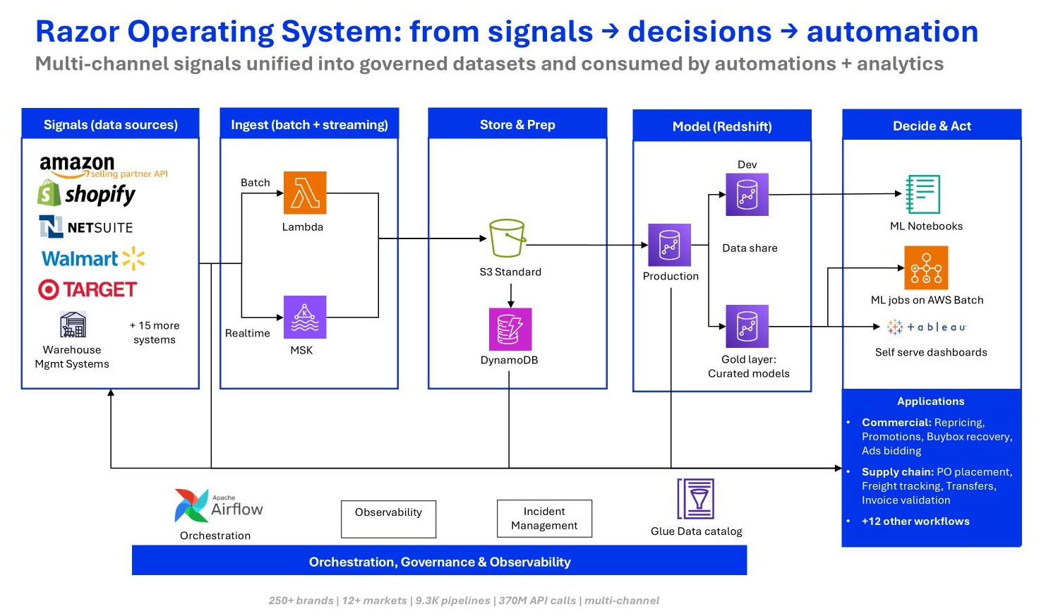
At the heart of this operation sits the Razor Operating System (ROS), a proprietary platform that processes 370M+ API calls monthly through 9,300+ data pipelines, transforming marketplace signals into automated actions at scale.
In this post, we share how Razor Group optimized their data platform by implementing a lakehouse architecture on AWS. We cover the architectural decisions, the phased migration approach, and the measurable business outcomes. Whether you’re looking to optimize workload performance, reduce infrastructure costs, or unlock multi-engine flexibility for your analytics, this blueprint provides actionable insights you can adapt for your organization.
The business challenge: Scaling data infrastructure for hypergrowth
As Razor Group’s brand portfolio expanded rapidly, the demands on their data platform grew significantly. The company needed their analytics infrastructure to keep pace with the speed of ecommerce, where pricing decisions, stock replenishment, and advertising bids happen in near real time.
Their existing architecture, built on Amazon Redshift provisioned clusters, had served them well during earlier growth stages. As workloads diversified and data volumes surged, several optimization opportunities emerged:
Figure 1: The Razor Operating System data architecture before the migration
Workload contention: Over 1,000 SQL models for ETL, transformation, and analytics competed for the same compute resources, creating resource contention during peak processing windows.
Cost-to-utilization mismatch: Always-on clusters ran 24/7, but workload analysis revealed that 98% of compute demand came from batch ETL rather than interactive analytics, which resulted in significant idle capacity during off-peak hours.
Data freshness gaps: Batch-oriented pipelines delivered data with 4–6 hour latency, limiting the team’s ability to react to fast-moving marketplace dynamics.
Scaling constraints: As concurrent users and pipeline complexity grew, vertical scaling alone couldn’t address the need for workload isolation and elastic capacity.
These weren’t failures of any single service. They were signals that the architecture needed to evolve to match the scale and diversity of Razor Group’s workloads.
Why a lakehouse architecture?
Rather than replacing their existing investments, Razor Group recognized the opportunity to optimize workload placement by adopting a modern lakehouse architecture. The core principles driving this decision:
Open table formats: Apache Iceberg provides ACID transactions, time travel, and schema evolution. Data is stored once and accessed by any compatible engine without duplication.
Elastic, per-workload scaling: With data persisted on Amazon Simple Storage Service (Amazon S3), each engine independently scales compute to match its workload. Each engine spins up for peak processing and scales to zero when idle, without over-provisioning shared infrastructure.
Multi-engine flexibility: Different workloads have different requirements. Heavy ETL benefits from distributed Spark processing, ad hoc exploration from serverless queries, and business intelligence (BI) dashboards from high-performance warehouse engines, each optimized for its purpose.
This approach allowed Razor Group to right-size each workload to the best-fit engine while maintaining a single, governed copy of data accessible across the entire platform.
Solution overview
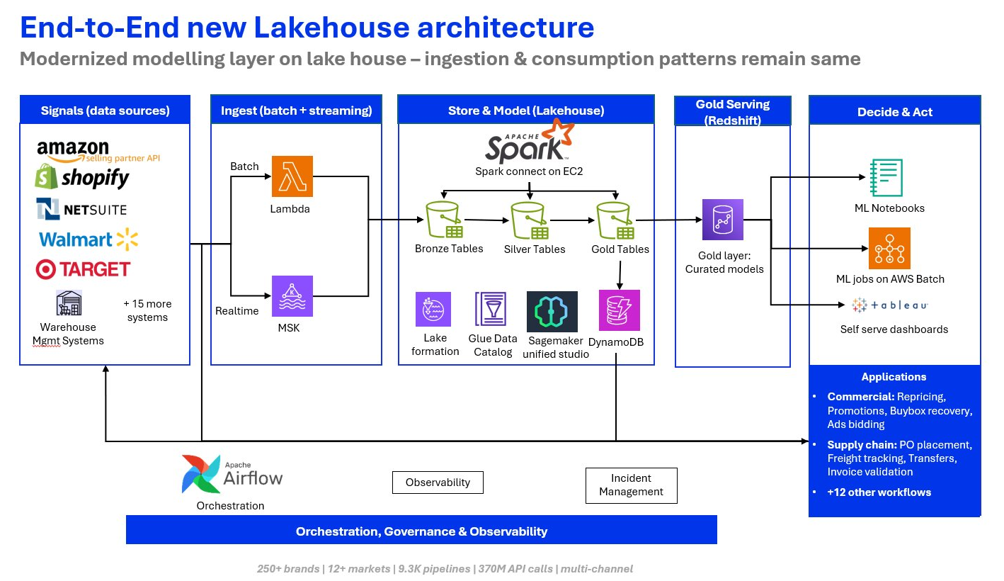
Razor Group partnered with AWS to implement a comprehensive lakehouse architecture that brings together multiple AWS services, each playing a complementary role:
Figure 2: End-to-end lakehouse architecture on AWS
Designing for scale: The lakehouse vision
The core insight driving Razor Group’s new architecture was simple: build a single, open format data lake that any engine can query. In the old model, each tool maintained its own copy of the data. In the new model, a single open-format data lake on Amazon S3 serves as the source of truth, and multiple purpose-built compute engines read from it based on the workload at hand.
This shift, commonly called a lakehouse architecture, combines the cost economics and scalability of a data lake with the query performance and governance of a data warehouse. Its open table format, Apache Iceberg, provides ACID transactions, schema evolution, time travel, and no vendor lock-in.
Storage and governance: The open data foundation
Amazon S3 Tables (a capability of Amazon S3) with Apache Iceberg — The primary storage layer, providing open-format tables with ACID transactions, partition evolution, and time travel. Data is stored once and accessible by any Iceberg-compatible engine.
AWS Glue Data Catalog — A unified metadata repository for consistent data discovery across all compute engines.
AWS Lake Formation — Fine-grained access control with column-level and row-level security so that governance scales with the platform.
Compute: Right engine for the right workload
Apache Spark on Amazon Elastic Compute Cloud (Amazon EC2) — Elastic, distributed compute for heavy ETL and transformation workloads. It uses AWS Graviton instances and Amazon EC2 Spot Instances for cost optimization.
Amazon Athena — Serverless SQL for ad hoc exploration and lightweight queries directly on Iceberg tables, with no infrastructure to manage.
Amazon Redshift Serverless — High-performance serving layer for BI dashboards, Tableau workloads, and interactive analytics. Amazon Redshift Serverless automatically scales to meet demand and pauses when idle, so it stays cost-efficient for the analytics workloads it serves best.
Orchestration and observability
Apache Airflow — Pipeline orchestration that manages 9,300+ data pipelines with dependency tracking and service level agreement (SLA) monitoring.
Comprehensive observability stack — Cost attribution, pipeline health monitoring, and data quality checks across all layers.
Note: When the architecture was originally designed, Amazon Redshift lacked Iceberg write support, making self-managed Spark the only viable ingestion path. This constraint has since been removed. Amazon Redshift now supports full Apache Iceberg DML (UPDATE, DELETE, MERGE), complementing its earlier CREATE/INSERT capabilities and AWS Glue Iceberg materialized views. This makes it a complete read/write Iceberg engine.
Migration approach
Rather than a risky big-bang cutover, Razor Group adopted a phased migration of five stages, each delivering standalone value while building the foundation for the next. Both Amazon Redshift and Spark pipelines ran in parallel during the transition, which maintained business continuity and let the team compare outputs with confidence. At no point was a production pipeline paused or a dashboard unavailable.
The migration journey: Five phases
The migration unfolded across five structured phases, each building on the previous one and delivering incremental value before the next began.
Phase 1: Establish the lakehouse foundation
Before migrating a single query, Razor Group needed to answer three questions: where does the data live, how is it managed, and how do we query it?
Why S3 Tables over self-managed Iceberg
Razor Group had already committed to Apache Iceberg as the table format: open, engine-agnostic, and equipped with ACID transactions and time travel. The question was whether to self-manage Iceberg on standard S3 buckets or use Amazon S3 Tables.
Self-managed Iceberg is powerful but operationally expensive. Someone has to run compaction jobs to prevent small-file proliferation. Someone has to expire old snapshots before metadata bloat degrades query planning. Someone has to clean up orphaned data files after interrupted writes. With 700+ models running across 40+ schemas, many of them materializing multiple times per day, that maintenance burden would scale with the platform rather than shrink.
S3 Tables eliminated this entire category of work. Compaction, snapshot management, and unreferenced file removal run continuously and automatically. The integrated Iceberg REST Catalog API means any compatible engine, such as Spark, Trino, Athena, Amazon Redshift, and Flink, can discover and query tables without maintaining a separate metastore. Discovery is unified through AWS Glue Data Catalog, which now exposes the Iceberg REST Catalog protocol as its access interface. Because tables are first-class AWS resources, access control, encryption, and lifecycle policies operate at the table level rather than through complex S3 bucket policies layered on top of file-path conventions.
For a company that didn’t want the operational burden of self-managing open table format maintenance, this was the deciding factor.
AWS Glue Data Catalog provides unified metadata discovery across all tiers. Lake Formation handles column- and table-level access control, with AWS Identity and Access Management (IAM) roles that follow least-privilege principles and AWS CloudTrail turned on for a full audit trail.
Choosing the query protocol
Prior to the rearchitecture, the Amazon Redshift cluster was 98% ETL, and only a fraction of compute hours were analyst SELECT queries. The replacement engine needed to handle both heavy batch transformations and interactive ad hoc queries.
Traditional Spark (spark-submit) handles batch ETL well, but couples clients to the cluster. Every job requires packaging driver JARs, managing classpaths, and submitting from within the cluster. For a platform running 200+ production directed acyclic graphs (DAGs) that process massive data volumes daily, this operational friction was a non-starter.
Spark Connect is the gRPC-based client-server protocol introduced in Spark 3.4, and it solved the coupling problem entirely. The cluster runs a persistent gRPC endpoint. Clients connect remotely and submit queries over the wire. Airflow operators become thin clients: they open a session, submit SQL, and get results, with success and failure mapping directly to task states. There are no driver JARs and no polling. Multiple consumers, including pipeline orchestrators, the web application, and developer notebooks, share one cluster without any of them needing Spark installed locally.
Deploying Spark Connect
Razor Group deployed a self-hosted Spark cluster on Amazon EC2: an on-demand AWS Graviton leader node, Spot workers at about 70% cost savings, and the Spark Connect endpoint exposed through an internal Network Load Balancer. Custom Amazon Machine Images (AMIs) bake in the full Spark, Iceberg, and S3 Tables stack, so private-subnet nodes have everything they need without internet access at runtime.
This phase produced no immediate business value, but it made everything that followed possible.
Phase 2: Migrate data ingestion
Razor Group’s ingestion layer pulls data from Amazon Selling Partner API, Seller Central portals, NetSuite ERP, and custom web scrapers. In the previous architecture, all of this landed in Amazon Redshift through COPY commands, which meant data freshness was dictated by batch job schedules and competed for resources on the same cluster that served analytical queries.
Razor Group migrated these pipelines to AWS Lambda functions orchestrated by Apache Airflow, writing data directly to S3 Tables in Iceberg format. The shift from schedule-driven to event-driven significantly improved freshness. Lambda functions spin up only when there’s data to process, and Airflow sensors trigger downstream transformations the moment new data lands. This replaced rigid hourly batch windows with data freshness measured in minutes.
The orchestration layer manages 200+ DAGs across 90+ flows and processes data from dozens of sources at scale. The migration required rewiring destinations from Amazon Redshift COPY to Iceberg writes, but the orchestration logic itself carried over with minimal changes.
This phase alone eliminated roughly 40% of compute costs by severing the always-on cluster dependency for ingestion.
Phase 3: Transform processing pipelines
This was the most technically demanding phase, and where Razor Group learned the most. The team migrated 1,000+ SQL models from Amazon Redshift to Apache Spark, working incrementally up the dependency chain across 40+ schemas. The models moved through a medallion structure: Bronze for raw ingested data, Silver for cleaned and conformed data, and Gold for business-ready aggregates.
Razor Group built automated conversion tooling and a validation framework that ran both Amazon Redshift and Spark outputs in parallel, comparing results row-by-row before decommissioning anything. Several categories of transformation pushed the limits of what automation could handle:
Window functions: The QUALIFY clause in Amazon Redshift has no Spark equivalent. Each instance required wrapping in a subquery with explicit row numbering, which affected dozens of models in the inventory schema alone.
JSON serialization: The most time-consuming category. Complex columns stored as JSON STRING in Amazon Redshift needed from_json() with hand-written STRUCT definitions in Spark. Every nested payload column across ads, orders, and transaction pipelines required schema introspection, with no shortcuts.
Function dialect: More than 20 function-level conversions, including NVL to COALESCE, DATEADD to interval arithmetic, and LISTAGG to ARRAY_JOIN(COLLECT_LIST()).
Snapshot elimination: The single biggest hidden cost. Full table copies that ran multiple times daily only to preserve point-in-time state consumed more than 35 hours of weekly Amazon Redshift compute. With Iceberg’s native time travel, these became zero-cost operations overnight.
When migrating 1,000+ SQL models, automated tooling handles the mechanical syntax conversions well. But roughly 30% of the models required human judgment: those with complex JSON payloads, deeply nested window functions, or cross-schema snapshot dependencies. These models consumed 70% of the migration effort.
Razor Group built a structured migration workflow that used Claude to accelerate this work: read source SQL, identify dependencies, convert syntax, resolve missing base tables, add JSON parsing, validate outputs, and write to the lakehouse. The system did more than translate SQL. It applied schema context, traced cross-model dependencies, and flagged edge cases that would have taken engineers hours to find manually. What could have been a multi-year effort became a systematic, repeatable process measured in weeks. This approach fundamentally changed the speed of migration.
Phase 4: Unify the serving layer
With data flowing through Iceberg tables, Razor Group collapsed the serving layer. End users query Gold-layer Iceberg tables through Amazon Redshift Serverless, and internal exploration and machine learning (ML) workloads read the same tables through Spark Connect. This removed the need to maintain separate data copies, materialized views, or extract jobs for different consumers.
This is the strategic payoff of an open table format. Iceberg tables on S3 are engine-agnostic: Spark for batch transforms today, Trino for interactive queries tomorrow, Flink for streaming next quarter. Any engine that speaks Iceberg can read the data without conversion or migration. Razor Group went from being locked into a single vendor’s SQL dialect to having the freedom to adopt new engines without touching the storage layer.
Phase 5: Operationalize and observe
The final phase made the lakehouse production-grade. Razor Group built a comprehensive observability stack that aggregates metrics, traces, and logs from every pipeline component into a unified view. This view supports centralized log search, anomaly detection, and automated alerting that correlates failures across the entire data platform.
This observability layer did more than provide visibility. It gave the team confidence. When you’re running thousands of pipeline executions daily, you need to know within minutes when something breaks, what caused it, and which downstream consumers are affected. That’s the difference between reactive firefighting and proactive operations.
Pipeline orchestration consolidated around three patterns: a daily pipeline (ingestion to materialization to export to AI agent analysis), an operations worker polling every 15 minutes, and weekly scraper jobs.
The cutover was zero-downtime by design: both schedulers ran in parallel for two weeks. Automated comparison checks validated that every pipeline produced identical outputs before the prior architecture system was disabled.
Results and business impact
The lakehouse architecture delivered measurable improvements across every dimension:
Metric
Before
After
Improvement
P95 query runtime
180 seconds
63 seconds
65% faster
Infrastructure cost
Always-on provisioned clusters
Elastic, workload-optimized
63% reduction
Data freshness
4–6 hour batch cycles
Event-driven pipelines
15-minute freshness
Concurrent capacity
Limited by cluster size
Elastic, independent scaling
Unlimited
Engine flexibility
Single engine
Multi-engine (Spark, Athena, Amazon Redshift)
Open format portability
The 63% reduction compares the lakehouse run-rate (January–March 2026) with the pre-rearchitecture run-rate (October–December 2025), the trailing three months before the rearchitecture. The figure is an apples-to-apples blended infrastructure number that includes compute and storage across both architectures. The before column covers Amazon Redshift cluster compute and managed storage. The after column covers Amazon EC2 (Spark workers, both on-demand and Spot), AWS Lambda, AWS Glue, Amazon Athena, Amazon Redshift Serverless, and S3 Tables storage. Data-transfer and ancillary services are excluded because they were not materially different between the two periods. Workload mix (the number of pipelines, models, and end-user query volume) was held broadly comparable across the two windows.
Lessons learned
Start with the decision loops, not the tools, and know your workload before you replace your warehouse.
The most valuable activity of the entire migration wasn’t writing a line of code. It was the Amazon Redshift workload analysis we ran before making any architectural decisions. Discovering that 98% of compute was ETL, with only a sliver going to analyst queries, validated the move to on-demand Spark. It also prevented us from over-provisioning the replacement infrastructure for interactive workloads that barely existed. Architecture decisions should always trace back to core business requirements: pricing accuracy, promotional responsiveness, intraday P&L visibility. Start there, not with the technology.
Design for multiple compute engines, and choose the right engine per workload.
One of the clearest lessons from running a single-engine architecture is what you give up. Avoid locking yourself into one compute layer for BI, ingestion, backfills, and ML alike, because they have fundamentally different cost and performance profiles. Iceberg, Spark, and S3 Tables work well together out of the box once you make the shift. The technology isn’t the hard part. The hard part is mapping 1,000+ models across 40+ schemas, tracing dependencies through 200+ DAGs, and discovering that a column is actually a JSON string silently serialized differently between two engines. Migration is as much an excavation project as an engineering one.
Automate conversion, but budget for the 30%.
Automated tooling handles mechanical syntax conversions well, and it should be the first tool you reach for. But models with complex JSON payloads, deeply nested window functions, or cross-schema snapshot dependencies require human judgment, and that work doesn’t compress. Roughly 30% of our models needed significant manual intervention, and those models consumed 70% of the total migration effort. Plan for it honestly from the start.
Observability must include cost attribution, and watch out for hidden cost bombs.
Snapshot operations were our biggest surprise. Full table copies that ran multiple times daily to preserve point-in-time state were costing more than 35 hours of weekly compute, and nobody questioned it because “that’s how snapshots work.” Iceberg’s time-travel capability eliminated their cost, and that single feature justified a meaningful portion of the migration on its own. More broadly, you cannot optimize what you cannot see, so track query-level usage and attribute it to teams and functions. Cost observability is not a nice-to-have. It’s foundational.
Governance isn’t optional. Build it into the foundation, and align stakeholders from day one.
Catalog and access control need to come first, before you scale adoption, not after. The same principle applies to people: migration is a cross-functional program, not an infrastructure project. Our two-week parallel run caught edge cases that row-level validation missed entirely: time zone differences between Amazon Redshift and Spark, partition pruning behavior under concurrent writes, and subtle ordering differences in non-deterministic window functions. That parallel run wasn’t a safety net. It was where the migration actually proved itself. None of it works without the right stakeholders involved and aligned from the very beginning.
Conclusion
Razor Group’s journey offers valuable lessons for organizations looking to optimize their data architectures:
Analyze your workload mix first. Understanding that 98% of compute was ETL rather than interactive queries guided the decision to offload heavy processing to elastic Spark, while preserving Amazon Redshift Serverless for the interactive analytics it handles best.
Design for multi-engine flexibility. Open table formats like Apache Iceberg eliminate the need to choose a single engine. Each workload runs on the engine best suited to its access pattern, cost profile, and performance requirements.
Automate migration, but budget for complexity. Automated transpilation handled 70% of SQL models, but the remaining 30% consumed 70% of engineering effort. Plan accordingly.
Observability must include cost attribution. Without per-workload cost visibility, optimization is guesswork. Razor Group discovered that Iceberg snapshot maintenance alone consumed more than 35 hours of compute weekly, a hidden cost that observability surfaced and automation resolved.
Build governance into the foundation.AWS Lake Formation and AWS Glue Data Catalog provided fine-grained access control from day one, not retrofitted after the migration.
Validate with parallel systems. A two-week parallel run between old and new architectures caught edge cases that automated testing missed, which supported a confident production cutover.
The road ahead
With the lakehouse foundation in place, Razor Group is positioned to accelerate innovation, from real-time pricing models to AI-driven inventory optimization, all powered by a unified, open, and governed data platform on AWS.
The company’s transformation demonstrates that modern data architectures aren’t about choosing between services. They’re about placing each workload where it performs best, using open formats to eliminate silos, and scaling each layer independently as the business grows.
Sending mass email campaigns presents significant challenges for many organizations. Enterprises often spend millions annually on proprietary email systems that are inflexible and expensive to maintain. These legacy platforms can restrict sending capacity, offer limited control, and require costly licensing agreements. The challenges intensify when handling large-scale communications like automated notifications, bulk marketing campaigns, and system-generated alerts. These scenarios create reliability issues, scaling limitations, and rising costs that impact teams’ ability to communicate effectively with customers.
Recently, a large federal organization faced similar challenges, spending over a million dollars annually on their email campaigns. By building a custom email solution on AWS, they sent a 2 million email campaign for approximately $300. This cost includes Amazon Simple Email Service (Amazon SES) and other AWS services. This transformation cut costs while providing the scalability and flexibility they needed for their growing campaign needs.
This transformation succeeded because building a cloud-native serverless mass email solution offers several advantages:
Cost optimization.
Pay only for email sent and actual compute resources used.
Remove costs associated with managing email servers.
Remove expensive licensing fees and maintenance overhead.
Scalability and reliability.
Automatically handle varying email volumes without infrastructure changes.
Support reliable delivery through built-in retry mechanisms and error handling.
Perform consistently during peak sending periods.
Security and compliance.
Secure access control through AWS Identity and Access Management (IAM) roles with least-privilege principles.
Comprehensive audit trails for all email campaigns with detailed logging to support your reporting requirements.
Detailed logging that customers can use for their compliance and reporting requirements.
Data encryption in transit and at rest that you can configure.
In this post, we explore the architecture of a cloud-native serverless mass email solution that integrates Amazon SES with AWS Step Functions, Amazon API Gateway, and Amazon DynamoDB. You will learn how these services work together to process email campaigns at scale while minimizing cost. Let’s get started!
Solution overview
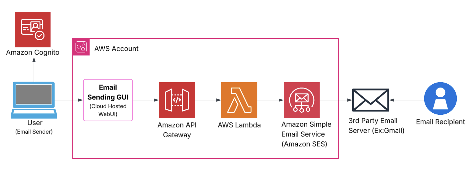
The serverless mass email solution consists of two main components: a user-friendly frontend interface and a scalable serverless backend. The frontend operates completely independently from the backend processing system, communicating through RESTful APIs from Amazon API Gateway. With this architecture, you can use the provided frontend interface as-is. Alternatively, you can integrate your own custom UI or existing applications while using the same backend email processing infrastructure.
The following diagram shows the complete architecture of the serverless mass email solution, including how the frontend and backend components connect through API Gateway to process email campaigns.
Figure 1: Complete architecture
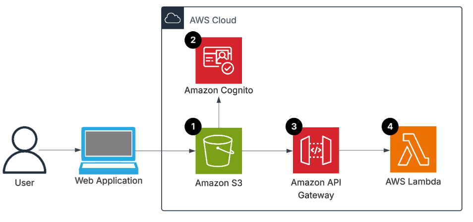
Frontend architecture and user flow
The frontend of the solution prioritizes usability while providing email campaign capabilities. Here’s how the components work together:
Figure 2: Frontend architecture of the SES email application
User authentication – Amazon Cognito handles authentication, providing secure user management and restricting access to authorized users.
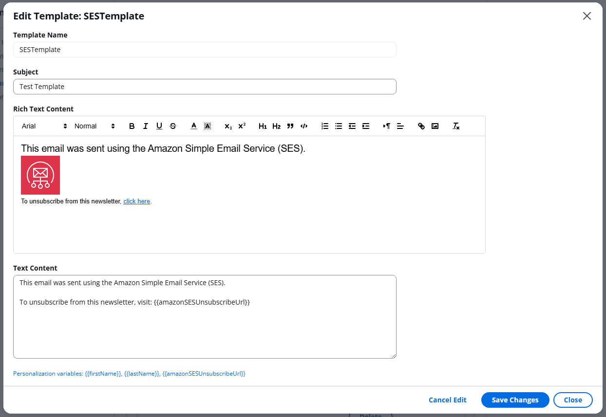
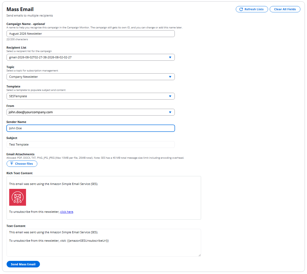
User interface – After successful authentication, users are redirected to a graphical user interface (GUI) where they can design and save email templates and launch large-scale campaigns (refer to figures 3 and 4).
Templates.
Amazon SES supports two types of templates: stored and inline. Stored templates live in SES, and you can reuse them across campaigns. With inline templates, you define the content and variables directly in the email sending request. Both approaches support dynamic personalization by replacing variables with recipient-specific data when the email is sent. For example, you can create a template that personalizes each email with the recipient’s name, custom offers, or any other dynamic content. For detailed information about template capabilities and personalization options, refer to the Amazon SES template documentation.
The following screenshots show the campaign interface, the template creation interface, and the campaign monitoring interface.
Figure 3: Email template creation interface
Figure 4: Mass email campaign interface
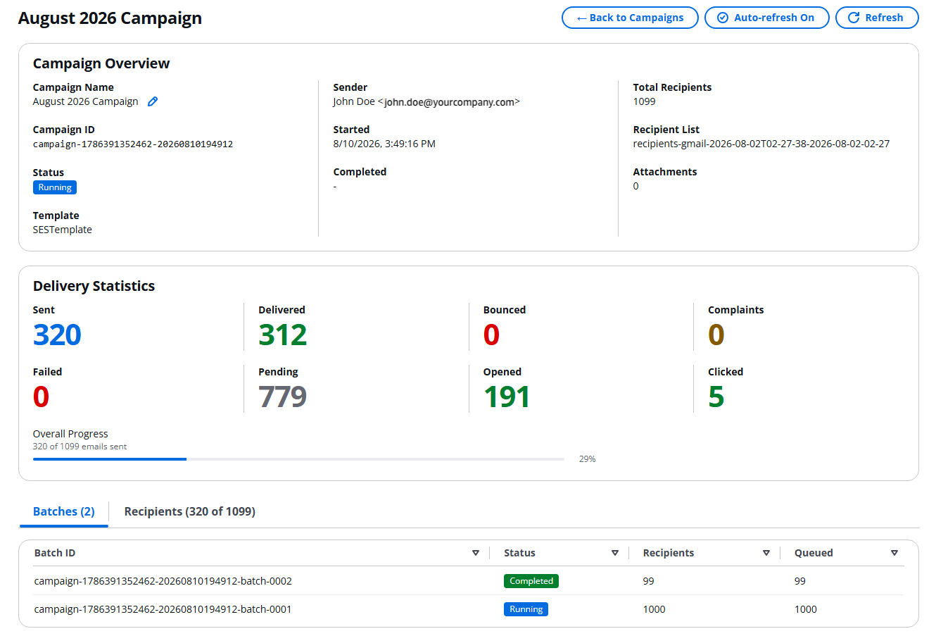
Figure 5: Campaign monitoring interface
Request processing – Each user action triggers a secure request through Amazon API Gateway to AWS Lambda functions, which then coordinate with our backend processing system.
From the user’s perspective, the experience is similar to using any standard email platform, with the added capability of handling campaigns at scale. This interface helps marketing teams, customer success managers, and business operations staff create and launch email campaigns directly through their browser, without needing to understand complex email protocols.
Backend architecture
After a user initiates an email campaign, our backend orchestrates a series of steps to facilitate reliable, large-scale email delivery. Let’s follow how an email campaign flows through the system:
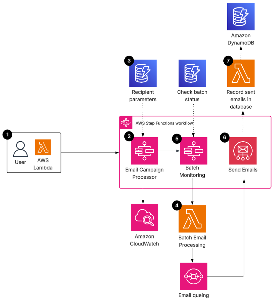
Figure 6: Backend architecture of the SES email application
As shown in the preceding figure, the backend processes email campaigns through the following steps:
Email campaign processor – When a user creates a new campaign through the GUI, a Lambda function processes the initial request, taking the user’s selected email template and campaign parameters. The function then triggers an AWS Step Functions workflow.
Workflow orchestration – The Step Functions workflow acts as the conductor and coordinates the entire email sending process. It initializes the campaign, sets up necessary configurations, and organizes the campaign into manageable batches.
Recipient processing – Before sending email, the Step Functions workflow retrieves recipient information, including the recipient’s name and email address, from DynamoDB and checks it for accurate delivery details.
Batch email processing – The Step Functions workflow begins organizing the email into manageable batches. The workflow queues these batches in Amazon Simple Queue Service (Amazon SQS), preparing them for processing.
Batch monitoring – As batches move through the system, Step Functions actively monitors their progress, tracking the status of each batch throughout the sending process.
Email sending – When SQS receives a message, it invokes a Lambda function that sends the email to Amazon SES for delivery. The function logs each delivery attempt in DynamoDB, with failed deliveries automatically returning to the SQS queue for retry attempts. It also records successful deliveries to support idempotency and prevent duplicate sends.
Record management – DynamoDB stores an audit trail that tracks both successful and failed delivery attempts, providing detailed logs to support reporting, campaign performance assessments, and compliance efforts.
Using these AWS services, the solution automatically scales from sending a few email to millions without manual intervention or infrastructure provisioning. You pay only for what you use, with no idle server costs. To demonstrate the cost-effectiveness of this architecture: sending 10,000 email costs approximately USD $4, including all AWS service charges. For current pricing details, refer to Amazon SES pricing.
To deploy this solution in your AWS account, refer to the source code on GitHub.
Conclusion
In this post, we explored the architecture of a scalable email sending solution using Amazon SES and other AWS serverless services. This architecture removes the complexity of traditional email infrastructure while providing capabilities for handling large-scale email campaigns. Whether you’re looking to modernize your existing email infrastructure or stand up a new solution, this serverless approach offers the ideal combination of streamlined design, scalability, and cost-effectiveness.
The Netflix experience is a journey of discovery. Every visual cue, from the artwork on a title to the video previews that autoplay while you browse, is there to connect you with a story you will love. We call these visual cues assets, and choosing the right one for each member is a personalization problem of its own. But which image or video preview of Squid Game should we show you? And what do we do right after a title launches, when there’s far too little interaction data to know which asset we should recommend to each member?
For years, our models answered the first question well and the second poorly. They learned which assets members interacted with, but treated every asset as an opaque ID, blind to what was actually in the artwork or video preview. Right after a title launched, its assets had no history, so we dialed up exploration on its assets to gather interaction data, and otherwise fell back to popularity heuristics that ignore your taste. Only once enough interactions had piled up could personalization take over. This is the classic cold-start problem.
This post shares how multimodal embeddings let our models see and hear the assets they recommend, so personalization can kick in far sooner, close to a title’s launch. Because a new asset arrives with its embedding the model already understands, that embedding carries member taste signals from related assets immediately. Consequently, the model needs far less interaction history before it can personalize. We cover three production systems, artwork personalization, query-aware artwork ranking, and video preview personalization, plus a cheap trick for choosing new embeddings before committing to full end-to-end integration and A/B testing.
Artwork Personalization
A single image is often a member’s first touchpoint with a title, so we create a diverse set of artworks for each title to appeal to different member tastes. We already use personalized artwork based on members’ interaction histories, but this approach breaks down for newer titles and their assets, where there is little or no behavioral data to learn from.
Making the Model See the Artwork
Our solution is to let the model “look” at the picture. We encode each artwork with CLIP, a pretrained image-text embedding model, and fold the result into how the model represents that asset, concatenating the per-asset CLIP image embedding, a 768-dimensional vector, with the asset’s learned ID embedding to give an asset representation:
e_id(a) is the asset’s learned ID embedding, and e_a is its CLIP image embedding. The two are concatenated and passed through an MLP layer to give h_a, the representation the model scores against a member.
This single change transforms how the model handles a brand-new artwork. Instead of treating it as an unseen ID, the model now receives a CLIP embedding the moment the asset is created. That allows a member’s preferences over visual themes, talent, and color palettes to be applied immediately, long before the asset accumulates any interactions of its own. Because those preferences are expressed in image-embedding space rather than tied to specific asset IDs, they transfer seamlessly across titles. If you consistently engage with artwork featuring a particular comedian, the model can carry that signal to their new title and prioritize the asset that places them front and center, even if it has never shown you that exact image before, as in the figure below. In this way, cold-start shifts from being a blind spot to something the embedding space already has an informed opinion about.
Knowledge transfer through CLIP embeddings. A member who has interacted with a comedian’s past stand-up artwork (left) leads the model to favor the new-title asset that features that comedian prominently (green check) over one that does not, even though it has never seen that specific image before.
From Five Models to One
That shift, from scoring an asset by the ID it happens to carry to scoring it by what the image actually contains, powers a second big win, model consolidation. Each title’s artwork spans multiple canvases with different croppings (billboard, vertical-box, horizontal-panel, short-panel, landscape-panel), and historically we trained a separate model per canvas, since an ID-based model has no way to know that the cropped and resized renderings of one scene are related, so signal could not flow between canvases and each faced its own cold-start.
CLIP embeddings break that barrier. Because they are largely invariant to crop, resize, and aspect ratio, those near-identical renderings map to nearly the same vector, as the figure further below shows. A single unified model can therefore pool interaction signal across every canvas, so a member’s affinity learned on a high-traffic canvas immediately informs the artwork we pick on a sparse one. The result is one model in place of five, with the largest gains on the canvases that have the least interaction data.
One source image, many canvases. The same Running Point artwork is cropped and resized across billboard, TV, mobile, and out-of-home placements, each with a different asset ID. Because CLIP embeddings barely change under crop and resize, a single unified model can personalize all of them.
Mixing Five Canvases of Training Data
Consolidation introduced a challenge that the per-canvas models never faced: how to effectively mix data across disparate canvases? The canvases differ widely in impression volume, and the interactions they log are not all worth the same to a member’s long-term experience. Training on pooled raw counts would let the highest-volume canvas and the most frequent interaction types dominate, so the low-data canvases we were trying to help would benefit least. Hand-tuning a weight per canvas would just trade that problem for a set of arbitrary hyperparameters and endless online sweeps to tune them.
Instead we use reward-based weighting, building on Netflix’slong-term reward modeling. Each training example is weighted by the long-term reward score attached to its interaction type:
a_ti is a training example, a positive interaction on asset i of title t. Its weight is set by the interaction type e observed on it, scored by ρ, that type’s long-term reward.
where e(·) is the type of the observed positive interaction and ρ is that type’s long-term reward score. Because interaction types are not distributed evenly across canvases, weighting by long-term value rebalances the canvas mixture on its own, with no weight set by hand. A canvas contributes in proportion to the long-term value of the interactions it drives rather than to how many impressions it happens to get. Consolidation becomes feasible, and the unified model optimizes for long-term member satisfaction instead of whichever short-term action is most frequent.
A Note on Offline Evaluation
Every result presented here must clear two bars: an offline metric evaluation followed by a large-scale online A/B test. The offline metric is the subtle one. Judging a new model on logs from the current production policy is biased, because that policy shows some assets far more often than others. The logged rewards describe what the policy preferred, not what members would have chosen from the full candidate set, so a new model that disagrees with the logging policy looks worse than it is, because the impressions it would have picked are barely represented in the data.
We handle this with inverse propensity scoring (IPS) computed on a dedicated slice of exploration traffic. A small fraction of traffic is served by a randomized policy that samples among a title’s candidate assets from a known distribution, so the propensity of showing a given asset in a given context is logged exactly at serving time rather than estimated after the fact. Reweighting every observation by the inverse of its logged propensity gives:
where D is the exploration slice and r(x, a) is the observed reward, such as a play. Impressions that exploration made rare are upweighted accordingly, and the estimator becomes an unbiased estimate of the reward a candidate policy would have earned had we actually deployed it. Having propensities that are known by construction, rather than modeled after the fact, is in our experience the single biggest reason our offline numbers track online outcomes. We report IPS as a ratio against the production baseline, and a candidate has to win there before it gets any A/B traffic.
Combining Both Ideas Works Better
Two ideas are bundled together here, so we ablated them separately against the old five-model production system.
V1, image embeddings only. The five per-canvas models kept as they were, each one augmented with image embeddings.
V2, unified model only. A single model trained over all five canvases, but with learned ID embeddings alone and no image content.
V3, both together. One unified model over all five canvases, with image embeddings in its asset representation.
As the chart below shows, each idea helped exactly where we expected: on the data-starved short-panel canvas and landscape-panel canvas. V3 was the clear winner. A change inside ±1% is not significant for this offline metric, and those bars are hatched in the chart. Most of what V1 and V2 do on their own sits inside that band.
Relative offline IPS lift by canvas for the three variants, each measured against the prior per-canvas model on that same canvas. Both ideas help where interaction data is scarcest, and V3 is strongest. Hatched bars fall inside the ±1% band, where the change in the offline metric is not significant; V3 values are labeled on the plot.
In the online A/B test across all device platforms, which ran for at least four weeks, the results drew a much clearer line: Neither idea moved our online core member metrics on its own. V1 and V2 were both flat and non-significant, and only V3 won a statistically significant lift. It is what runs in production today.
The two ingredients need each other. V1 tells a per-canvas model what an asset looks like, but one sparse canvas has too few examples to teach it how to use that. V2 supplies plenty of data, but only ID-based data, which a new asset lacks. V3 has both, so mature canvases teach the shared model how CLIP embeddings map to member preference and that mapping transfers straight to the sparse ones. The effects compound rather than add, since the V3 short-panel lift (5.691%) exceeds V1 and V2 combined. The lesson is to look for a second blocking factor before concluding that content features do not help.
Cold-Start Challenge from a New UI Launch
The real test came from the product change that motivated the work. Netflix was preparing its largest TV home-screen redesign in a decade, which would make short-panel the dominant artwork canvas effectively overnight. This was a cold-start problem in its sharpest form. The canvas about to receive the most impressions had the least historical data, and waiting for short-panel interactions to accumulate would have degraded the user experience. Consolidation lets short-panel selection draw on signal pooled from every canvas, and CLIP embeddings let the unified model personalize a short-panel asset that has gathered very few interactions of its own.
We shipped V3 ahead of the launch and measured it with a month-long holdback A/B test, keeping a small control group on the prior per-canvas model. V3 absorbed the shift immediately, with statistically significant gains on both our core discovery metric and streaming hours, and larger gains than in the steady-state ablation. That stronger result is what we expected, since a sudden shift in which canvas dominates is exactly where V3 should help most.
Query-Aware Artwork Personalization
Your general taste is the right signal when browsing, but not when searching. For example, when searching for a specific actor, you want artwork that features them, even if your broader taste says otherwise. On the Netflix Search Page, the member’s intent is explicit and stated in the query, and the displayed artwork should reflect it.
The same CLIP embeddings we added for cold-start hand us this almost for free. Because CLIP projects text and images into one shared embedding space, we can measure how well a query matches a candidate artwork directly by the cosine similarity between the CLIP text embedding of the query and the CLIP image embedding of the asset. We blend that alignment term with the usual personalization score:
Here the personalization term is the score the artwork model above already produces for a member and asset, the second term compares the text embedding of the query against the image embedding of the asset, and the mixing weight α between 0 and 1 is tuned through online A/B testing. The first term is “what we think you like”; the second is “what you just asked for,” and α sets how much each matters.
Crucially, this took no extra modeling effort. The CLIP embeddings already sit in the asset representation from the artwork work above, so they carry the text-image alignment for free, and we get a query-aware ranker by adding a single similarity term at scoring time. The effect is visible in the search results themselves.
Query-aware artwork for a search for a specific actor. Each result surfaces an asset that visually features the searched actor, aligning the artwork with the member’s explicit intent.
Personalizing Video Previews via MediaFM
Video previews raise the bar over still artwork. A video preview unfolds over time, and its appeal comes as much from motion, pacing, dialogue, and soundtrack as from any single frame. Our older video preview personalization models saw none of that. Like the early artwork models, they treated each preview as an opaque ID. Our first content-aware attempt, SeqCLIP, described a video preview by its frames, encoding each with a CLIP embedding and then averaging them into one vector. That captured what a video preview looked like, but a mean of still frames still misses what it sounds like, the dialogue and music that carry so much of a preview’s tone.
To capture the rest, we turned to MediaFM, Netflix’s first in-house multimodal foundation model. Trained on 80 million shots, MediaFM fuses the following three signals per shot into a single embedding:
Visual: SeqCLIP
Audio: Apretrained speech and audio embedding model
Text: Captions encoded via a large-scale text model
Adopting MediaFM required no new infrastructure, since we simply integrate its shot embeddings into the asset representation, exactly as we did with CLIP embeddings for artwork.
The added modalities paid off. We evaluated both embeddings against the ID-only baseline offline with IPS and then in a five-week online A/B test across all device platforms, and both signals gave the same ordering, MediaFM > SeqCLIP > ID-only, and each step of added content awareness helped, with the gains largest on TV. Offline, both content-aware embeddings beat the ID-only baseline on IPS and MediaFM beat SeqCLIP, as the chart below shows. Online, MediaFM came out on top too, delivering a statistically significant lift in our core streaming metric over the ID-only baseline and outperforming SeqCLIP. This shows that the audio and timed-text signals, which a visual-only encoder like SeqCLIP cannot capture, add real value. We have since shipped MediaFM as the default video preview embedding across all platforms.
Relative offline IPS lift for the two content-aware video preview embeddings, each measured against the ID-only baseline at the zero rule. Adding visual content awareness helps, and adding audio and timed text on top of it helps further.
Choosing Embeddings Cheaply with a Proxy Task
New embeddings arrive constantly, but end-to-end trials are expensive, which cost data engineering, model retraining, and weeks of A/B test traffic. We couldn’t afford to run the full pipeline for every candidate, so we gated the funnel with a cheap question:
From the content embedding alone, can you predict which asset wins under a plain, unpersonalized policy?
We first select a fixed set of titles. For each title we use exploration data to find its debiased popularity winner, the asset with the highest interaction rate after we adjust for how often it was shown using its propensity score. We mark this winner with a binary label, 1 for the winner and 0 otherwise. We then train a linear probe to recover that label from the asset embedding alone, with no title, cast, or metadata, by minimizing the standard binary cross-entropy loss:
Keeping the probe linear and embedding-only is intentional, since it isolates how much of an asset’s popularity is actually encoded in the embedding. If the embedding captures the semantic drivers of popularity, a simple linear classifier should be able to identify likely winners. If it does not, the probe performs no better than random guessing, which is the baseline we score it against.
We first used the linear probe to screen and prune a broad set of candidate embeddings before modifying any production pipeline, narrowing the field to two finalists, SeqCLIP and the leading MediaFM variant. We then carried both through full offline evaluation and online A/B testing. All three signals, the linear probe accuracies, the offline IPS lifts, and the online A/B results, ranked MediaFM ahead of SeqCLIP, as the chart below shows. That alignment is why the linear probe now gates every new MediaFM version before release.
Linear probe Δaccuracy, offline IPS lift, and online A/B metric lift for the two finalists. All three agree that MediaFM beats SeqCLIP. The online panel is measured against the ID-based baseline, with its values withheld.
The Netflix Embedding Store
None of this would be practical without shared infrastructure. Every embedding in this post, CLIP for artwork, SeqCLIP and MediaFM for video previews, lives in the Netflix Embedding Store, a component of Netflix’s AI Platform that hosts dense embeddings for titles, games, member profiles and multimedia assets. A foundation model encodes raw asset content into a dense vector once, and the Embedding Store serves that vector to every downstream system, the artwork model, the query-aware ranker, the video preview model, and others, through the same interface. Crucially, it serves the exact same embeddings at training time and at online inference time, so there is no skew between what a model learns from and what it sees in production.
Its key property is that it decouples foundation-model updates from personalization-model deployments. A new embedding, or a new version of an existing one, can be registered, backfilled across the catalog, and validated entirely on its own, without touching the training or serving code of any model that consumes it. Once it is in the Embedding Store, it becomes available to every ranking and personalization model through configuration alone, no downstream code changes, no coordinated release. This is what let us swap CLIP into the artwork model, stand up the query-aware ranker on the same vectors, and roll MediaFM through the video preview model, each as an independent change rather than a cross-team migration.
Foundation-model embeddings (CLIP, SeqCLIP, MediaFM) are stored once and consumed by every downstream system: artwork, query-aware artwork, video previews, and other rankers.
What We Learned, and What’s Next
Three lessons stood out.
Pretrained CLIP embeddings let us consolidate five artwork models into one while boosting performance on data-starved canvases. This benefit became especially clear when the redesigned TV home screen rolled out.
For video, multimodality wins decisively. The audio and text signals that a purely visual encoder cannot access pushed MediaFM past SeqCLIP.
A cheap proxy task yields big savings, efficiently pruning the candidate set before running full end-to-end experiments and online A/B tests.
Next, we aim to extend the Embedding Store toward a single shared semantic space for image, text, and video. Such a unified representation would enable cross-modal retrieval, such as matching a video preview to a search query, or a static artwork to the video preview it was derived from, as well as unified asset ranking across surface types and a more cohesive, intuitive discovery experience for members everywhere.
Acknowledgements
We thank Aneesh Vartakavi, Santiago Castro, and Avneesh Saluja for the CLIP embedding and MediaFM work that made the content-aware models described here possible, and Ratna Kavuri for the backend systems that serve multimedia personalization in production.
To provide the best experiences, we use technologies like cookies to store and/or access device information. Consenting to these technologies will allow us to process data such as browsing behavior or unique IDs on this site. Not consenting or withdrawing consent, may adversely affect certain features and functions.
Functional
Always active
The technical storage or access is strictly necessary for the legitimate purpose of enabling the use of a specific service explicitly requested by the subscriber or user, or for the sole purpose of carrying out the transmission of a communication over an electronic communications network.
Preferences
The technical storage or access is necessary for the legitimate purpose of storing preferences that are not requested by the subscriber or user.
Statistics
The technical storage or access that is used exclusively for statistical purposes.The technical storage or access that is used exclusively for anonymous statistical purposes. Without a subpoena, voluntary compliance on the part of your Internet Service Provider, or additional records from a third party, information stored or retrieved for this purpose alone cannot usually be used to identify you.
Marketing
The technical storage or access is required to create user profiles to send advertising, or to track the user on a website or across several websites for similar marketing purposes.