Post Syndicated from Explosm.net original https://explosm.net/comics/boner
New Cyanide and Happiness Comic
Post Syndicated from Explosm.net original https://explosm.net/comics/boner
New Cyanide and Happiness Comic
Post Syndicated from xkcd.com original https://store.xkcd.com/

Post Syndicated from xkcd.com original https://xkcd.com/3288/

Post Syndicated from Grab Tech original https://engineering.grab.com/jarvis-pro-route-firsr-answer-later
The first Jarvis Pro prototype could produce answers that sounded right.
That was the problem.
One early answer looked polished: it named the merchant, summarized the week, and recommended pushing promotions before the next review. It was also wrong. The merchant’s order volume was down, but the sharper issue was operational: more outlets were paused and fulfilment had slipped. Sending more demand into that setup would have made the merchant look worse.
That failure changed how we judged the system. Fluent was not enough.
Jarvis Pro is the AI assistant we built for Grab account managers. Its job is to help them turn account data into better merchant conversations: what changed, why it changed, and what to do next. They rarely ask clean dashboard questions. They ask: “I am meeting this merchant tomorrow. What should I tell them?” or “Which accounts in my portfolio need attention this week?”
Those questions hide decisions: scope, access, business diagnosis, and metric definition. If the system gets those wrong, confidence becomes a liability.
So the core design became: route first, answer later.
In an internal offline evaluation (not a measure of production performance or business impact), routing matched the expected safe route for 99.4% of 351 realistic prompts drawn from labelled eval sets from the first half of 2026. In a focused portfolio and brand answer-quality suite, the average score moved from 78.5 to 91.0. These figures come from offline launch-readiness evaluation only; they are not business-impact proof.
A dashboard answers a bounded question:
“Show net sales for merchant X last week.”
An account review question has to diagnose the work to be done:
“This merchant softened this week. Should I push promos, ads, or operations fixes before the review?”
If outlets were paused, more traffic can backfire. If average order value fell, the next action may be menu or bundle design. If a dashboard, warehouse table, and local spreadsheet disagree, the first task is metric reconciliation, not recommendation.
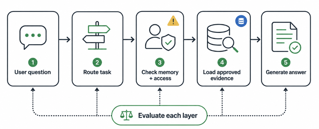
We wanted Jarvis Pro to classify the task first, then load only the context needed for that task.
The launch router was a prompted LLM classification step constrained by a routing guide: supported task types, allowed context, answer shapes, and conditions that should force a handoff or refusal.
A broad merchant review routes differently from an ads campaign recap or an out-of-scope request. A route is not just a label; it decides the structure, metrics, tool path, and guardrails.
Here is a simplified example. The merchant and numbers are illustrative.
User prompt
I am seeing Merchant A soften this week. I need talking points for tomorrow’s review. Should I push promos, ads, or operations fixes?
Router decision
Ilustrative example only. No actual, live, or non-public data was used.
{
  "route": "brand_performance_action_plan",
  "scope": {"merchant": "Merchant A", "country": "Singapore"},
  "memory": "use current question context",
  "context": ["brand action plan", "approved metric catalog", "ads context"],
  "guardrails": ["no private competitor metrics", "no unsupported projection"]
}
Answer extract
Merchant A’s issue looks like order volume, not basket size. Net sales fell 7.8% week-on-week and orders fell 9.1%, while average order value increased 1.4%.
Start with operations before promotions. Temporary pause rate rose from 2.1% to 4.8%, and fulfilment fell from 94.6% to 91.8%. Extra demand may leak unless the merchant fixes availability first.
Talking point: “Before we add promo depth, let’s recover lost availability. If we bring pause rate back below 2.5%, we should have a cleaner read on whether the remaining gap is demand, menu, or ads.”
The route prevented three common mistakes: jumping straight to discounts, inventing competitor spend, and answering from a generic growth template.
Here, “memory” means saved user context such as country, role, portfolio scope, and preferences. That context is useful when a user says “my portfolio”. It is risky when saved defaults override explicit context, missing identity becomes a guess, or a memory request crosses user boundaries.
We put memory before answer generation and kept the decision small: proceed, ask for onboarding information, prefer explicit context, use saved defaults, look up portfolio scope, or refuse. Backend permissions and row-level controls remain the authorization layer.
That extra checking costs time. Jarvis Pro does route classification, memory checking, context selection, warehouse or specialist tool calls, then generation. To keep the wait usable, we loaded route-specific context, ran memory before expensive retrieval, consolidated warehouse queries, capped tool calls, and returned unavailable cells as N/A instead of looping until the conversation stalled.
That tradeoff was deliberate: a slower first token was better than a fast unsafe recommendation.
Even with good routing and memory, an assistant is only as good as the numbers it pulls.
When a user says “the number is wrong”, several failures can look identical: wrong source, different metric definitions, different entity mapping, or stale data. One reconciliation pass showed that what looked like model error was sometimes just a freshness mismatch between reporting surfaces.
We built regression checks that normalised source values and compared daily rows across approved metric paths. The point was not the row count. It was knowing whether to fix source selection, metric guidance, or the caveat shown to the account manager.
One aggregate score would have hidden the failures we cared about.
The routing set had 351 prompts labelled against the routing guide. Each prompt had an expected route family, meaning the broad business category, plus an expected route and any handoff or refusal. “Accepted route accuracy” meant the selected route was exact or semantically equivalent and safe. A wrong business family, missed handoff, or unsafe scope failed.
The answer-quality suite had 501 total cases scored on a 0-100 rubric covering template fit, metric use, diagnosis, next action quality, caveats, and guardrail compliance. Within that suite, the 150-case portfolio and brand subset improved from 78.5 to 91.0. A wrong merchant, wrong country, fabricated metric, unsupported projection, or private competitor detail could fail a case. User isolation was treated as a hard evaluation requirement. All scores were measured offline against fixed rubrics for launch readiness; they do not reflect production commercial outcomes.
That caught the answer we most wanted to avoid: plausible, polished, and operationally unsafe.
The final paragraph is too late to resolve ambiguity. Jarvis Pro has to earn the right to answer: route the task, check memory and access, load the right evidence, cap the tools, then judge failures at each layer.
Offline evals gave us confidence in system behaviour, not commercial uplift. Measuring that needs production telemetry: recommendations shown, actions taken, accounts affected, and outcomes.
The assistant should not merely sound like a great account manager. It should first prove it understands the account.
Grab is Southeast Asia’s leading superapp, serving over 900 cities across eight countries (Cambodia, Indonesia, Malaysia, Myanmar, the Philippines, Singapore, Thailand, and Vietnam). Through a single platform, millions of users access mobility, delivery, and digital financial services, including ride-hailing, food delivery, payments, lending, and digital banking via GXS Bank and GXBank. Founded in 2012, Grab’s mission is to drive Southeast Asia forward by creating economic empowerment for everyone while delivering sustainable financial performance and positive social impact.
Powered by technology and driven by heart, our mission is to drive Southeast Asia forward by creating economic empowerment for everyone. If this mission speaks to you, join our team today!
Post Syndicated from Eric Smith original https://www.servethehome.com/kioxia-cd9p-7-68tb-e3-s-nvme-ssd-review-fast-gen5-storage/
We test the Kioxia CD9P (CD9P-R) in its 7.68TB E3.S configuration to see how the new PCIe Gen5 NVMe SSD performs on different architectures
The post Kioxia CD9P 7.68TB E3.S NVMe SSD Review Fast Gen5 Storage appeared first on ServeTheHome.
Post Syndicated from The Atlantic original https://www.youtube.com/shorts/7Z711ASVwrs
Post Syndicated from Gokul Govindaraju original https://aws.amazon.com/blogs/compute/amazon-linux-default-ssm-parameter-will-now-track-the-latest-kernel/
Today we are announcing that the Amazon Linux kernel-default AWS Systems Manager (SSM) parameter will now update to point to the latest Amazon Linux kernel version as new kernel versions get released. On August 17, 2026, for Amazon Linux 2023 (AL2023), the SSM parameter was updated from kernel 6.1 to kernel 6.18. As new kernel versions get released (expected annually), the parameter will continue to update to the latest kernel version after a validation period.
This post explains the default kernel behavior, what it means for your workloads, and how to manage the transition.
Amazon Linux ships multiple kernel versions and has tracked a default kernel for each OS version. For example,
the AL2023 parameter:
ssm:/aws/service/ami-amazon-linux-latest/al2023-ami-{minimal}-kernel-default-{x86_64 arm64}
has remained on kernel 6.1 since launch. Going forward, the kernel-default SSM parameter will update to the latest kernel as new versions are released. Each new kernel will go through a 3- to 6-month validation period after GA before we update the default. This window gives you time to test the new kernel before the change. We will announce the kernel-default upgrade date before it takes effect.
| SSM Parameter | Resolved to (Before) | Resolves to (Now) |
al2023-ami-{minimal}-kernel-default-{x86_64, arm64} |
Kernel 6.1 AMI | Kernel 6.18 AMI (what’s changed) |
al2023-ami-{minimal}-kernel-6.18-{x86_64, arm64} |
Kernel 6.18 AMI | Kernel 6.18 AMI (unchanged) |
al2023-ami-{minimal}-kernel-6.1-{x86_64, arm64} |
Kernel 6.1 AMI | Kernel 6.1 AMI (unchanged) |
Note: Already-running instances will keep the kernel they booted with and are not affected by this change. Only new instances launched from the kernel-default parameter will boot kernel 6.18. If you already use a version-specific SSM parameter, nothing changes for you.
The Linux kernel is the foundation of workloads you run on Amazon Elastic Compute Cloud (Amazon EC2) and other services. Each new kernel brings meaningful improvements. For example, kernel 6.18 includes the Earliest Eligible Virtual Deadline First (EEVDF) CPU scheduler for fairer CPU time distribution and improved latency in mixed workloads. The kernel also increases Transmission Control Protocol (TCP) receive buffer for better network throughput on high-bandwidth instances.
Previously, customers who wanted to run the latest Amazon Linux kernel had to manually update their SSM parameter references and redeploy each time a new kernel became available. With this change, you can receive these improvements without needing to manually upgrade.
Staying on the default kernel is the recommended approach as it allows your new instances to always run the latest validated kernel with no manual intervention. However, because the default will now advance annually, you should build processes to validate that the new kernel works for your workload before each upgrade takes effect. If your workload has specific requirements that mandate a fixed kernel version, evaluate whether the new default is compatible or revert to a kernel version that suits your use case.
If you haven’t validated kernel 6.18 yet, we recommend launching test instances on kernel 6.18 using the version-specific SSM parameter al2023-ami-{minimal}-kernel-6.18-{x86_64, arm64}. For instructions on referencing SSM parameters in your launch configuration, see the AL2023 User Guide.
If you experience issues with the new default, or if your workload requires a specific kernel version for additional validation time or any other reason, revert to the version-specific SSM parameter. Change your references from al2023-ami-{minimal}-kernel-default-x86_64 to al2023-ami-{minimal}-kernel-{kernel_version}-x86_64 (for example, al2023-ami-kernel-6.1-x86_64). This applies anywhere you resolve an AL2023 AMI, including AWS CloudFormation templates, launch templates, Amazon EC2 Auto Scaling groups, CI/CD pipelines, or CLI scripts. For examples, refer to the AL2023 User Guide.
Each of the supported kernels (6.1, 6.12, and 6.18) continue to receive updates as defined in AL2023 kernel lifecycle. When staying on a specific version, we recommend tracking the kernel lifecycle and planning upgrades before the kernel reaches end of support.
Note: For Federal Information Processing Standards (FIPS) workloads, the default kernel may not always be the FIPS-validated kernel. If you require FIPS mode, see AL2023 FIPS FAQ.
In this post, we announced that the Amazon Linux default SSM parameter will now upgrade to the latest kernel as new kernel versions are released. The AL2023 kernel-default parameter was updated from kernel 6.1 to kernel 6.18 on August 17, 2026. We explained how the new cadence works, how already-running instances are unaffected, and how to stay on a specific kernel version if your workload requires it.
To learn more, see the AL2023 Kernel documentation and the AL2023 release notes. For questions or issues, contact AWS Support.
Post Syndicated from jzb original https://lwn.net/Articles/1083090/
Quickshell is a toolkit for
building desktop components, such as toolbars or menus. It uses QML, which is a declarative language
for designing GUI applications. Quickshell helps developers create graphical tools
for common desktop use cases with a focus on ease of development. It offers a
convenient method for writing user interfaces and has been adopted by a number
of projects, such as caelestia-shell and DankMaterialShell, that
provide desktop environments for minimal window managers like Sway and niri.
Post Syndicated from Nidhi Nayak original https://aws.amazon.com/blogs/big-data/long-term-system-tables-retention-in-amazon-redshift-with-amazon-s3-tables/
Amazon Redshift system tables capture a continuous stream of operational signals: every query that runs, every connection that is made. This data powers observability, performance analysis, and compliance auditing across your data warehouses. Until now, the system tables retained this critical data for only 7 days, making long-term compliance and auditing difficult without custom workarounds.
Amazon Redshift system table integration with Amazon S3 Tables, a capability of Amazon Simple Storage Service (Amazon S3), automatically delivers your system table logs data to Amazon S3 Tables and stores them in Apache Iceberg format. You can configure retention periods for Amazon Redshift system table beyond the current 7-day limit, giving you extended compliance, auditing, and cross-warehouse observability without custom ETL pipelines or cluster resource consumption. Your data is open, durable, and queryable from Amazon Redshift, Amazon Athena, AWS Glue, Amazon EMR, or other Apache Iceberg-compatible engines.
In this post, we walk through how the Amazon Redshift system table integration delivers log data to Amazon S3 Tables. This feature is supported on RA3 and RG provisioned clusters and Amazon Redshift Serverless workgroups.
If you run Amazon Redshift, you often face operational challenges driven by the 7-day system table retention limit:
Amazon Redshift system tables integration with Amazon S3 Tables is a fully managed capability that automatically writes Amazon Redshift system table data to Amazon S3 tables in Apache Iceberg format. AWS handles partitioning, compression, and retention management automatically. The log writing process runs in an isolated background process that alleviates resource contention with production workloads. AWS manages the pipelines for you.
The feature supports over 25 system views at launch – see the supported system views documentation.
Follow these steps to enable system table integration with Amazon S3 Tables from the Amazon Redshift console:
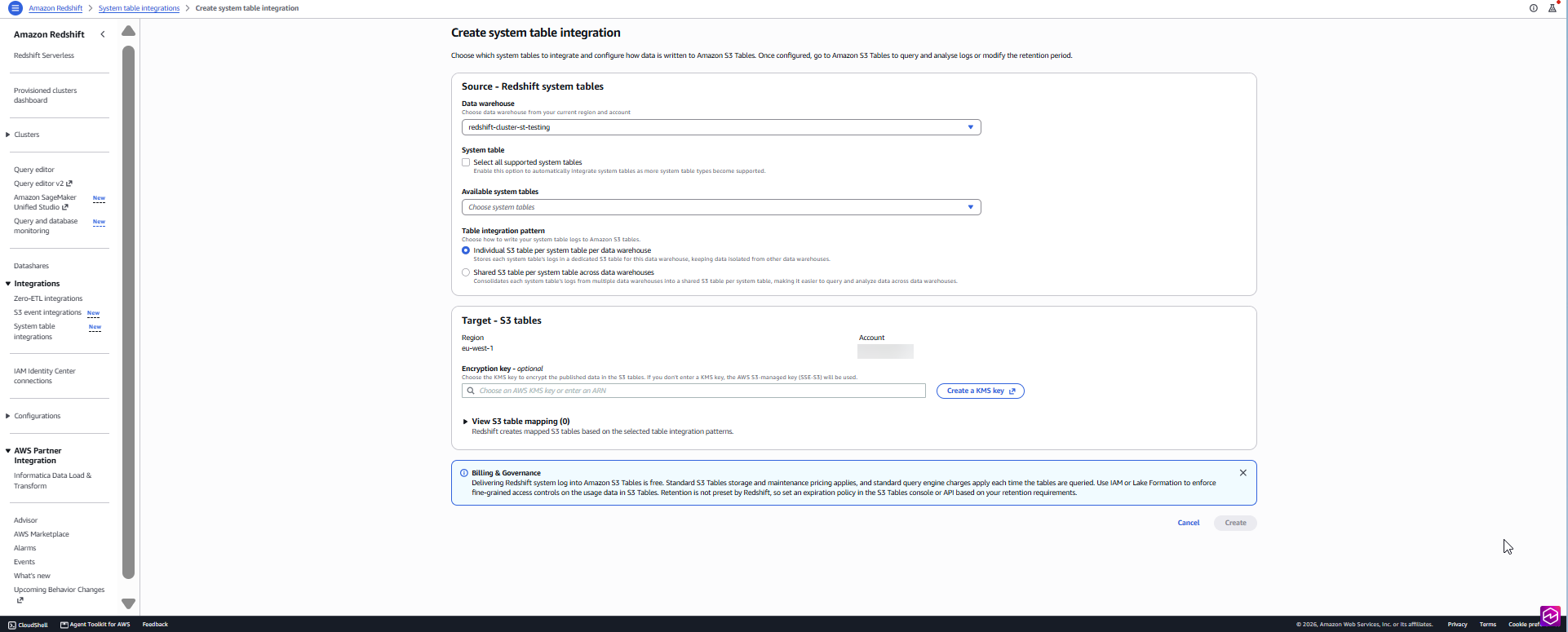
Figure 1: Selecting the Amazon Redshift data warehouse in the System table integration wizard
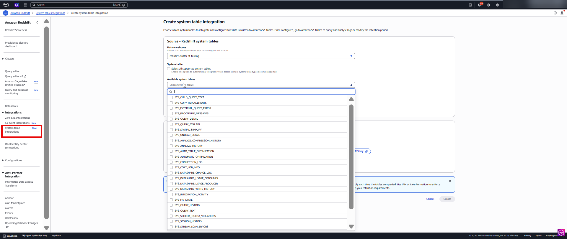
Figure 2: Choosing the system views to publish from the Available system tables list
To verify the integration is active:
After it’s enabled, Amazon Redshift writes log data to Amazon S3 tables periodically through an isolated background process, separate from production workloads. To start querying the retained logs, you will need to perform a one-time setup that connects your Amazon Redshift environment to Amazon S3 Tables data through AWS Glue Catalog. Complete the following steps:
Because access to Amazon S3 Tables is read-only, the integrity of your audit trails is inherently preserved.
For detailed setup instructions including IAM policy examples, see Registering the S3 Tables bucket with AWS Glue Data Catalog.
Your system table data is stored in Apache Iceberg, an open table format, so you have the freedom to choose a compatible query engine. Your observability and auditing data works with the tool you already use.
You can analyze your operational data using:
Because the data is stored in open Apache Iceberg format in Amazon S3 Tables, you can query it with Amazon Redshift, Amazon Athena, AI agent skills for natural-language queries, Amazon SageMaker Unified Studio, an Iceberg-compatible engine, business intelligence (BI) tools, and observability systems.
Log delivery from Amazon Redshift to Amazon S3 Tables incurs no additional cost. You only pay for Amazon S3 Tables storage, maintenance, and querying the data with the engine of your choice.
The following scenarios illustrate how Amazon Redshift system tables integration with Amazon S3 Tables addresses common operational, compliance, and observability challenges across your Amazon Redshift environment. We also built a dedicated skill, querying-aws-redshift, for this feature and embedded it into the AWS MCP Server so you can query Amazon Redshift system tables from Amazon S3 Tables.
With months or years of SYS_QUERY_HISTORY data retained, you can trace how individual queries perform over extended periods. You can compare execution time, queue time, and resource consumption for a query across days, weeks, or months.
You can pinpoint exactly when performance started degrading and correlate it with what changed: a new schema, a spike in data volume, or an additional concurrent workload. Extended retention turns troubleshooting into proactive, data-driven root cause analysis.
Every workload change affects your system: a new ETL pipeline, an instance type change, a Workload Management (WLM) queue adjustment, or a new team of analysts running ad hoc queries. The question is always: how did this change affect performance?
With Amazon S3 Tables integration for Amazon Redshift system table, you can make data-driven decisions with confidence. Query SYS_QUERY_HISTORY to compare execution times, queue wait durations, and concurrency scaling events from the weeks before a change versus the weeks after. If you onboarded a new reporting workload two weeks ago and want to understand its effect on existing queries, the data to confirm that is already there, with zero custom pipeline required.
Your system table data is stored in Apache Iceberg and cataloged in AWS Glue, which means an observability or business intelligence (BI) tool that reads Apache Iceberg can connect directly to it. Visualize workload distribution trends in Amazon Quick Sight for executive reporting. Use Amazon SageMaker Unified Studio for deeper analytical exploration or to power AI-driven insights from your operational data. Beyond AWS services, connect your preferred third-party observability systems and BI tools to track query volumes, monitor connection patterns, set up alerts for anomalies, or correlate Amazon Redshift operational data alongside application-level logs.
Your observability and auditing data works with tools that you already use. Direct access to durable, structured operational data, with a tool you prefer.
Workload demand varies throughout the year. Month-end close, quarter-end reporting, annual planning cycles, and promotional events all create predictable usage spikes, but only if you have enough historical data to see the pattern.
With extended retention, you can analyze utilization trends across multiple business cycles. Identify when you consistently approach capacity limits, measure how demand shifts quarter over quarter, and validate whether your provisioned resources align with actual usage.
For regulated industries, extended retention delivers a fully managed audit trail with built-in integrity.
SYS_CONNECTION_LOG records every authentication attempt. SYS_USERLOG captures user account changes. SYS_QUERY_HISTORY documents every query executed against your warehouse.
Configure retention to match your organization’s data retention policies: whether that is 90 days, one year, or multiple years. The read-only access policy helps prevent records from being altered after they are written, including by administrators.
If you run multiple Amazon Redshift warehouses, you benefit from a unified view of operational data. The feature supports two deployment patterns to match your organizational structure:
UNION operation is required.warehouse_name column. Filter by warehouse for instant cross-cluster analysis.warehouse_account_id, warehouse_region_name, warehouse_namespace_arn, warehouse_name, and s3_tables_ingestion_time to reduce scan scope and improve performance. This is particularly important when querying large volumes of historical data across multiple warehouses.Amazon Redshift system table integration with Amazon S3 Tables replaces custom ETL pipelines with a fully managed solution to preserve your Amazon Redshift operational data. With automatic Apache Iceberg-based storage, open format queryability, and built-in audit integrity, you get months or years of observability data, fully managed. You can enable it through the AWS Management Console, AWS Command Line Interface (AWS CLI), or AWS SDKs.
To learn more, visit the Amazon Redshift system tables documentation.
Post Syndicated from Preetkumar Shah original https://aws.amazon.com/blogs/security/aws-network-firewall-now-supports-rule-hit-count/
As firewall rule sets grow in complexity, security teams face a common challenge: manual log analysis is used to determine which rules are actively matching traffic and which are consuming capacity without being triggered. This lack of visibility creates operational and compliance gaps. Organizations with governance policies that require removal of dormant rules after a defined period have no mechanism to identify them. Teams responsible for compliance frameworks such as Payment Card Industry (PCI) 4.0 and Digital Operational Resilience Act (DORA) can’t provide evidence that specific controls are actively functioning. Central teams managing firewalls on behalf of multiple business units have no way to determine which rules are unused or need updating.
In this post, you learn how a new AWS Network Firewall capability—rule hit count—addresses these challenges by providing traffic match data for stateful rules across both custom and managed rule groups. With this data, you can identify and remove unused rules, accelerate incident response, and validate security control effectiveness for compliance.
Rule hit counts track how often each stateful rule matches network traffic. The hit counter increments only when a rule match results in an alert log being created. This means any rule with an alert, drop, or reject action will increment the hit counter, because these actions generate alert logs. However, rules configured with a pass action don’t generate alert logs by default, meaning they won’t appear in the rule hit count metric.
To gain visibility into traffic matching pass rules, you can include the alert keyword within the pass rule. This generates an alert log while still permitting the traffic to its intended destination. The following Suricata rule demonstrates this approach:
This rule passes HTTPS traffic to its destination while also generating an alert log, making sure the rule appears in the hit count metric.
The rule hit count feature adds the following metadata to each alert log. Metadata is included by default and doesn’t require additional configuration:
“aws_metadata": { “resource_arn": “arn:aws:network-firewall:us-east-1:123456789012:stateful-rulegroup/StatefulRuleGroup” }
The following example shows a complete alert log with this metadata included:
The alert log data in the preceding example is the source for rule hit count metrics. Network Firewall pushes these alert logs to your Amazon CloudWatch Logs or Amazon Simple Storage Service (Amazon S3). To identify the specific rule that generated an alert, you can search using the combination of the sid (signature ID) and resource_arn fields. The firewall monitoring dashboard uses these fields to generate hit counts for each rule, so you can review rule activity directly on the dashboard without querying logs.
You can also access and analyze this data by querying those logs directly using CloudWatch Logs Insights for logs stored in CloudWatch, or Amazon Athena for logs stored in Amazon S3.
Network Firewall rule hit count is enabled by default, so you don’t need to perform any additional configuration to start tracking rule hits on your firewall policies. This means that as soon as you deploy your firewall rules, you can begin to monitor which rules are being triggered, helping you gain visibility into your traffic patterns and identify potential security concerns.
This walkthrough requires an existing network firewall configured to inspect traffic from your Amazon Virtual Private Cloud (Amazon VPC). If you don’t have one set up yet, follow the Getting started with AWS Network Firewall guide.
Additionally, ensure the following:
pass action don’t generate alert logs by default. To track pass rule activity in the hit count metric, include the alert keyword in your pass rules, as demonstrated in the How it works section of this post.The Top Rule Hits dashboard shows aggregated hit counts per firewall across all Availability Zones within the AWS Region where that firewall is deployed. To view rule hit count metrics, open the Network Firewall console and select your firewall. Navigate to the Monitoring and observability section. Under Top analysis, you will see the Top Rule Hits metric. Select a lookback period to view rule activity within that timeframe.
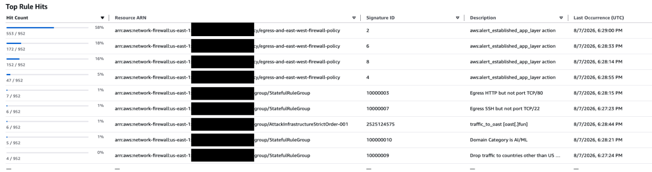
Figure 1: Rule hit count from the dashboard
Figure 1 shows the Top Rule Hits panel from the AWS Network Firewall console, displaying the most frequently triggered stateful rules. It includes columns for Hit Count (with bar chart and fraction), percentage of total hits, Resource ARN, Signature ID, Description (the msg field from the Suricata rule), and Last Occurrence (UTC).
Signature IDs 2, 4, 6, and 8 are system-generated signatures corresponding to the firewall policy’s strict order default actions. Because these signatures originate from the policy rather than a rule group, the resource_arn field displays the firewall policy Amazon Resource Name (ARN) instead of a rule group ARN. They appear in the Top Rule Hits when the policy has default actions such as Drop established, Alert established, or their application-layer variants configured. These signatures fire on established connection packets that don’t match any explicit rule, enforcing the policy’s default deny posture.
The following examples demonstrate how rule hit counts help you address common operational challenges.
msg field from the Suricata rule) that actively matched traffic during the selected lookback period. Any rule in your firewall policy whose signature ID doesn’t appear in this metric hasn’t matched any traffic during the specified timeframe. These rules are either stale or not ordered correctly within your rule group.traffic_to_oast [oast[.]fun]) with six hits and a last occurrence of August 7, 2026, at 6:28:44 PM UTC. This rule is detecting traffic to an out-of-band application security testing (OAST) domain, which could indicate an attacker attempting to exfiltrate data or validate a vulnerability in your environment. By filtering the top rule hits metric to the timeframe of a suspected incident, your team can quickly identify this type of suspicious activity and scope the impact without manually parsing thousands of log entries.Domain Category is AI/ML) with five hits and a last occurrence of August 7, 2026, at 6:28:21 PM UTC. After adding this rule to monitor or restrict traffic to AI/ML related domains, the hit count confirms the rule is actively matching traffic as intended. Similarly, signature ID 100000009 (Drop traffic to countries other than US) shows four hits, validating that the geofencing rule is functioning and blocking outbound connections to destinations outside the United States. These hit counts provide security teams with concrete evidence that newly deployed controls are working. Rule hit counts are included with Network Firewall at no additional cost. However, standard charges apply for storing and querying log data. If you configure log delivery to CloudWatch Logs, CloudWatch pricing applies. If you store logs in Amazon S3 and query them with Athena, standard Amazon S3 storage and Athena query charges apply. For complete pricing details, see AWS Network Firewall pricing.
Keep the following in mind when you use rule hit counts:
In this post, you learned how rule hit counts in AWS Network Firewall give you visibility into your firewall rule utilization and effectiveness. By tracking how frequently each rule matches traffic, you can identify unused or redundant rules, optimize rule ordering, validate security controls for compliance, and respond faster during security investigations. For more information, see AWS Network Firewall.
If you have feedback about this post, submit comments in the Comments section below.
Post Syndicated from Bruce Schneier original https://www.schneier.com/blog/archives/2026/08/detailed-timeline-of-openais-cyberattack-on-hugging-face.html
OpenAI presented details of its AI’s model’s cyberattack on Hugging Face at Black Hat last week. Simon Willison details the timeline. It’s really interesting to read through—and really impressive cyberoffense work.
Post Syndicated from Miller Vargas original https://blog.cloudflare.com/task-based-oauth-consent/
Since June, developers have created thousands of third-party OAuth apps on Cloudflare, with more than a million authorizations since.
OAuth makes delegated access possible. It lets applications act on a user’s behalf without asking them to handle long-lived credentials or hand over a password. That model works well when an application can describe its access needs with a small set of scopes.
Developers use OAuth for SaaS integrations, internal tools, CLIs, and agents. Our permission model has become more granular over time to support better scoping of these different workflows. That is great for security, but it makes a purely all-or-nothing consent screen hard to justify.
Cloudflare OAuth already allows clients to request a subset of their configured scopes. But once the client made that request, the user could not narrow it any further on the consent screen. For the user on the consent screen, the experience was still an all-or-nothing one. If an application requested more access than a user was comfortable granting, their only options were to approve the full request, or deny outright.
MCP servers are a good example of this. An MCP server might request a broad set of permissions, because in theory an agent could use all of them. But most users would not want an agent to have that much access. Before this feature, the only way to handle this was for the app developer to build a custom scope selection screen before sending the user to our consent flow.
Today, we’re introducing OAuth scope customization. Client owners can mark specific scopes as optional when configuring an OAuth client, giving users the ability to grant a narrower subset of an application’s requested access at authorization time.
The OAuth spec already allows authorization servers to grant a narrower set of scopes than what was requested. We built on top of that flexibility to make this work cleanly for every existing app.
Our goal with introducing scope selection is to give security conscious users more flexibility to make the right choices for their use case, without turning the consent screen into a long scope checklist.
With scope customization:
One important detail is that required and optional scopes are evaluated only against the scopes requested in a specific authorization flow, not every scope configured on the client. That matters because OAuth clients do not always request their full configured scope set.
For example, a client might be configured with user-details.read, workers-scripts.write, workers-kv-storage.write, and zone.read, while marking workers-kv-storage.write and zone.read as optional. If that client starts an authorization flow requesting all four scopes, the consent screen will evaluate all four. In that case, user-details.read and workers-scripts.write remain required, while the user can choose whether to grant workers-kv-storage.write and zone.read.
But if the client later requests only workers-scripts.write and zone.read, then only those two scopes are considered for that authorization flow. user-details.read and workers-kv-storage.write would not be shown or enforced, because they were not requested.
This keeps the consent screen focused on the task at hand, rather than every capability the application could request. It also means existing OAuth clients keep their current behavior by default: if a client does not opt into optional scopes, the consent flow remains unchanged.
Developers can opt into scope customization when configuring an OAuth client. Scopes continue to be configured as they are today, and clients can now additionally specify which of those scopes are optional:
In the example above, the client can request all four scopes, but the user may only opt out of the workers-kv-storage.write and zone.read scopes during consent. user-details:read and workers-scripts.write remain required if they are included in the authorization request.
If the client later requests only workers-scripts.write and zone.read, then only those two scopes are considered for that authorization flow. user-details.read and workers-kv-storage.write would not be shown or enforced because it was not requested.
When a user deselects any optional scopes and completes the authorization flow, the generated access token will only contain the scopes they consented to. For developers, this means you need to check the granted scope set after exchanging the authorization code, rather than assuming the full requested set of scopes was approved.
An app that handles a narrower grant gracefully, for example an agent that operates within whatever subset of permissions it receives, is one that users feel comfortable authorizing. Requesting only the permissions needed and marking the rest as optional is a good sign to users that your app respects their access decisions.
Over the next few weeks, we will be expanding our account & zone-level role surface to cover nearly every Cloudflare product. That means more API token roles, account membership options, and OAuth scopes, giving customers the tools to secure workloads with the right level of access.
Allowing developers and users to better restrict access through optional OAuth scopes is an important step toward a more flexible and trustworthy consent experience on Cloudflare. With optional scopes, developers can build more nuanced authorization flows, and users gain more control over what they approve.
To get started with Third Party OAuth, take a look at our documentation or jump straight to the OAuth apps page in the dashboard and create your first OAuth app.
This feature is one of the many that we built with the help of our 1,111 interns. Congratulations to Miller Vargas and José Enrique Rodriguez on your high impact contributions here. Miller is a senior at the University of Texas – Austin studying computer science and math; and José is a senior at Universidad Panamericana studying engineering, data intelligence, and cybersecurity.
Post Syndicated from Nisha Gambhir original https://aws.amazon.com/blogs/big-data/track-sagemaker-unified-studio-project-costs-with-custom-tags-and-aws-cur/
Organizations running machine learning (ML), analytics, and generative AI workloads on Amazon SageMaker Unified Studio domains and projects face a common cost governance challenge. System tags (AmazonDataZoneDomainId and AmazonDataZoneProject) are automatically propagated to all underlying project resources. However, custom tags such as CostCenter, Team, or Environment are not propagated to dynamic resources created through the Studio UI. This creates a gap when you need to report project costs grouped by custom tags.
In this post, we walk through a serverless solution that bridges this gap by enriching AWS Cost and Usage Report (CUR) data with custom project tags. By the end of this post, you can build an Amazon Quick Sight dashboard to filter and analyze Amazon SageMaker Unified Studio project costs by any custom tag dimension that you define. This gives your team the visibility to make informed spending decisions.
The solution consists of three automated subsystems:
The following diagram shows the end-to-end architecture:
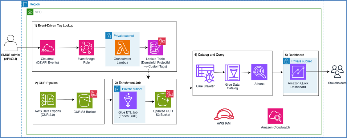
Figure 1: SageMaker Unified Studio project custom tag cost reporting
The workflow is as follows:
Before deploying this solution, you need:
You configure custom tags on project profiles through the Amazon DataZone API. First, enable custom tags on your project profile:
When creating or updating a project, set the tag values:
Important: The AmazonSageMakerProvisioning-<domainAccountId> role needs an inline policy that permits your custom tag keys. Without this, project environment deployment fails.
The following is the inline policy that’s used for the custom tags shared in this post:
Activate the SageMaker Unified Studio system tags as cost allocation tags so they appear in CUR data:
These tags take up to 24 hours to start appearing in CUR reports after activation.
The solution is packaged as a CDK application. Clone the GitHub repository and deploy:
This creates the following resources:
CreateProject/UpdateProject/DeleteProject events.Note: The solution uses serverless components (Lambda, DynamoDB on-demand, AWS Glue, Amazon Quick Sight), so you only pay for what you use. The primary cost drivers are AWS Glue ETL job execution time and Amazon Quick Sight SPICE storage.
Create a CUR 2.0 export through AWS Data Exports that delivers Parquet files to the CUR S3 bucket created by the stack. The following screenshots show the complete configuration process in the AWS Billing and Cost Management console.
To create the export, follow these steps:
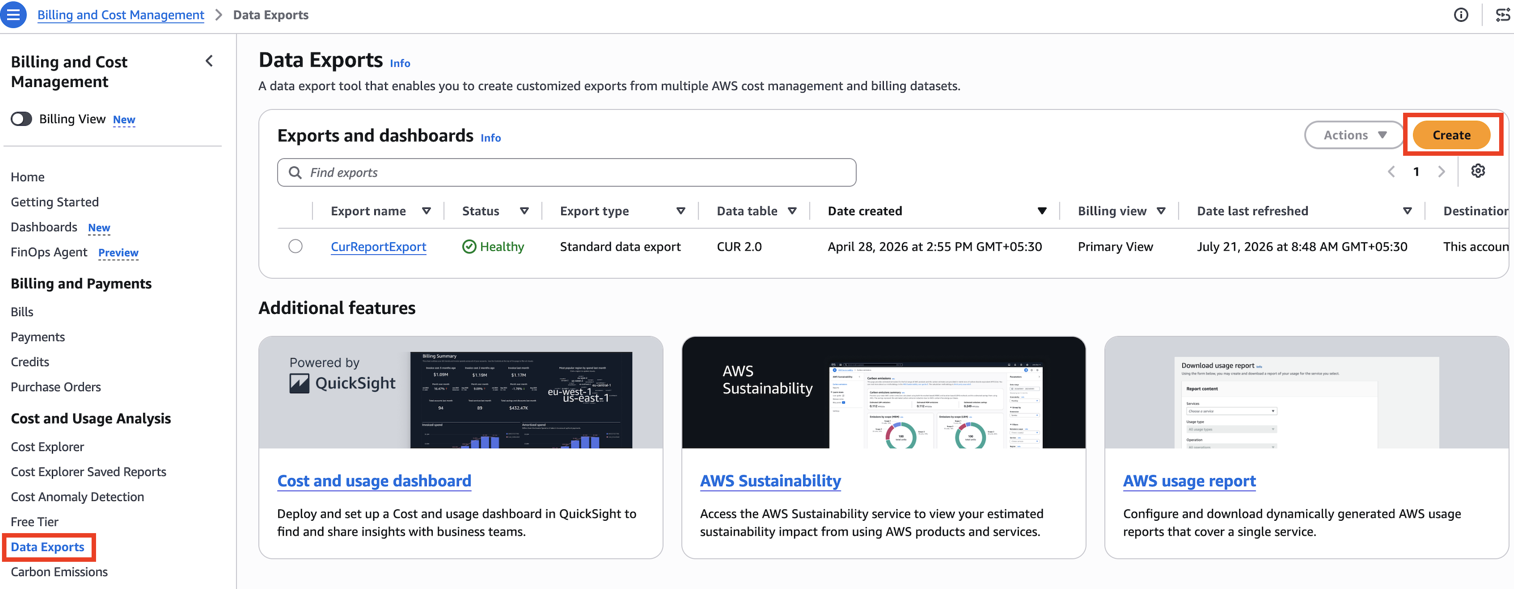
Figure 2: Data Exports page listing existing exports
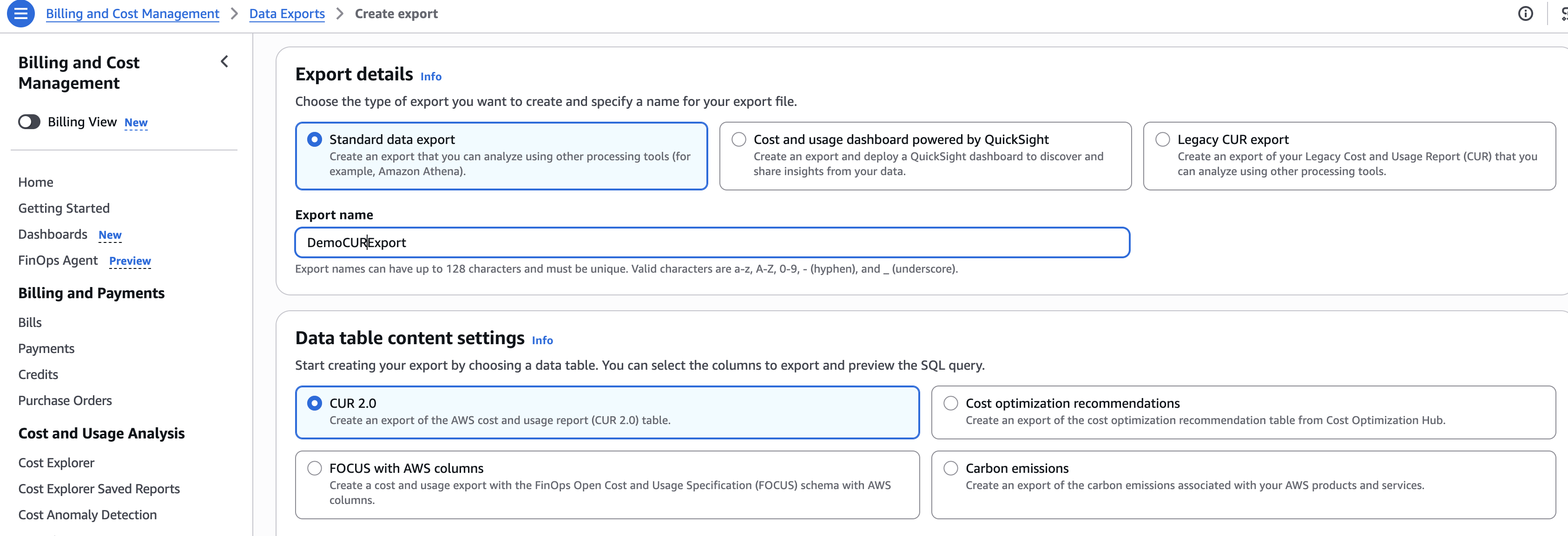
Figure 3: Create export page with Standard data export and CUR 2.0 selected
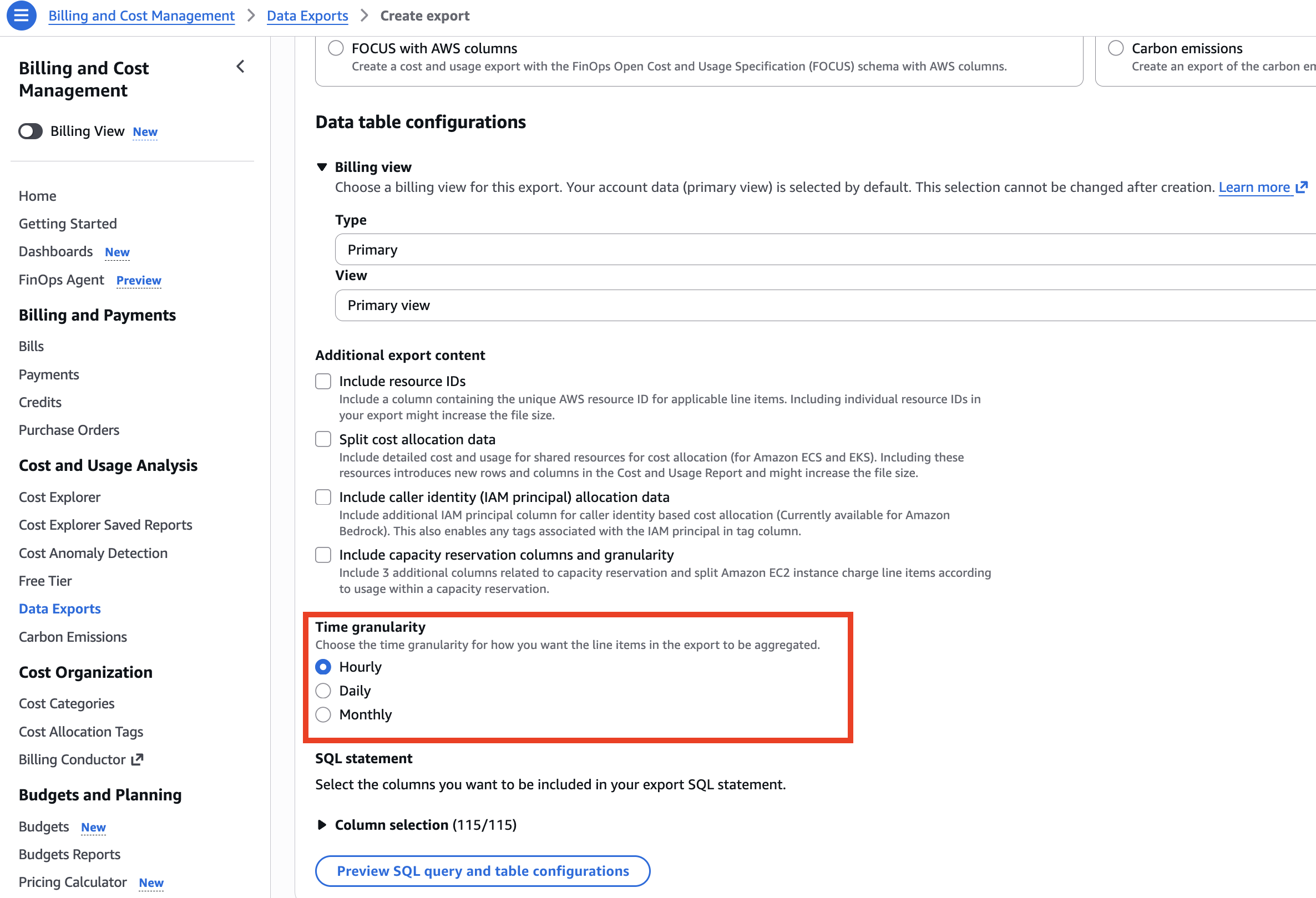
Figure 4: Data table configurations with time granularity set to Hourly
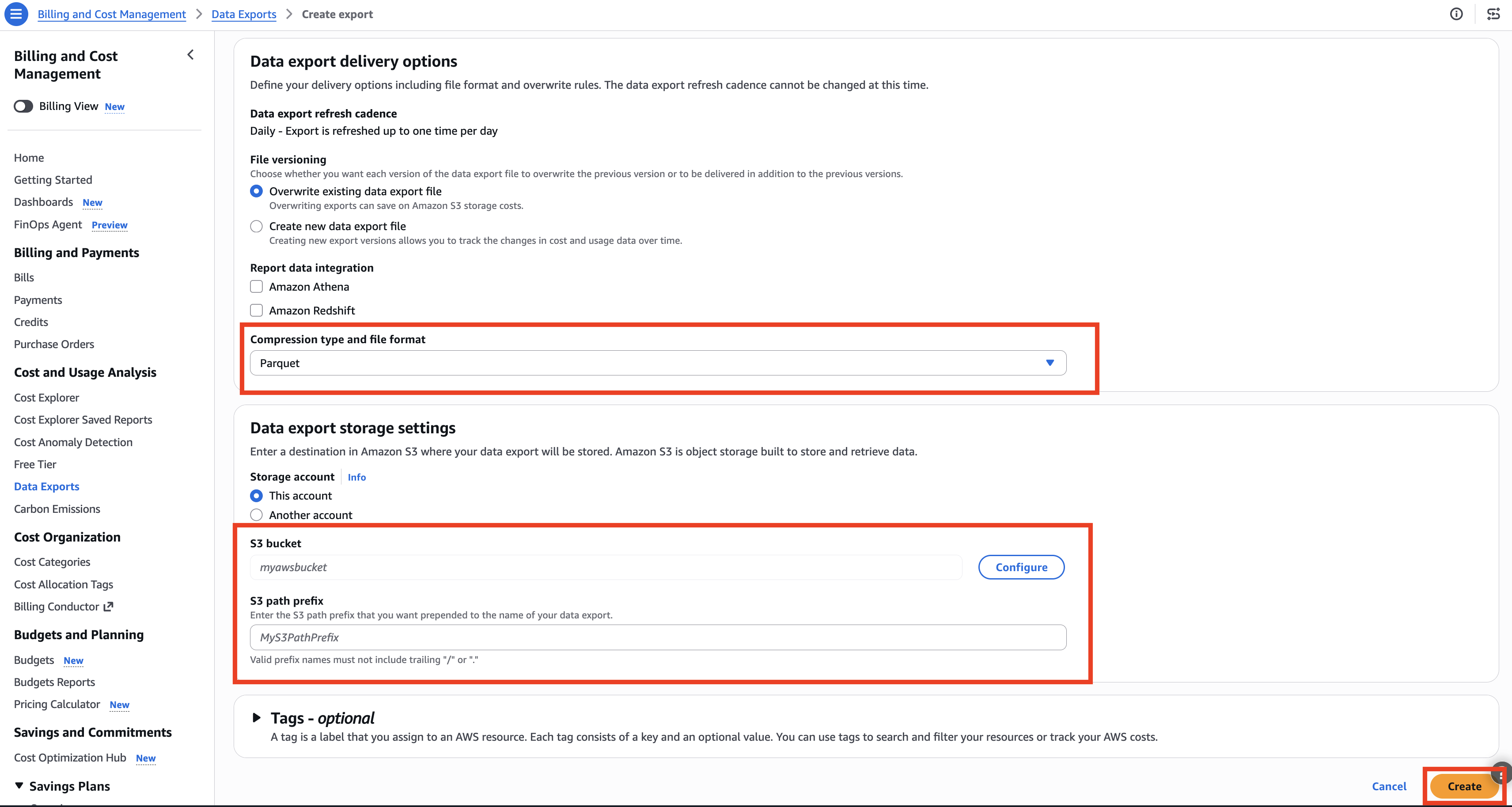
Figure 5: Data export delivery options with Parquet format and S3 storage settings
When a project is created or updated in Amazon SageMaker Unified Studio (through the Studio UI or API), the following happens automatically:
The Lambda function reads tags directly from the responseElements.resourceTags field of the CloudTrail event rather than making a separate GetProject API call. This avoids a race condition where GetProject might return empty tags while the project is in the UPDATING state.
The AWS Glue ETL job runs on a schedule (after each CUR delivery):
Line items without a matching project in the lookup table retain all original columns with NULL custom tag values. No data is dropped.
After the first ETL run and crawler execution, set up the Amazon Quick Sight dashboard:
This creates a dashboard with five visuals:
And six interactive list filters: Domain, Project, CostCenter, Team, Environment, Service.
The custom SQL includes a CASE statement for service categorization:
After deploying the infrastructure and setting up the dashboard, verify that each component of the pipeline is functioning correctly.
SmusCostReporting-ProjectTagRule).The DynamoDB lookup table uses a simple key schema:
| Attribute | Type | Role |
| domainId | String | Partition Key |
| projectId | String | Sort Key |
| CostCenter | String | Custom tag |
| Team | String | Custom tag |
| Environment | String | Custom tag |
Custom tags are stored as dynamic attributes. Any tag key set on a project becomes a column in the table.
SmusCostReporting-ProjectTagsTable).You should see rows with your custom tag values populated in the costcenter, team, and environment columns.
Figure 6 shows the Amazon Quick Sight dashboard with two side-by-side horizontal bar charts: Cost by Cost Center and Cost by Project. Domain Name and Project Name list filters appear at the top.
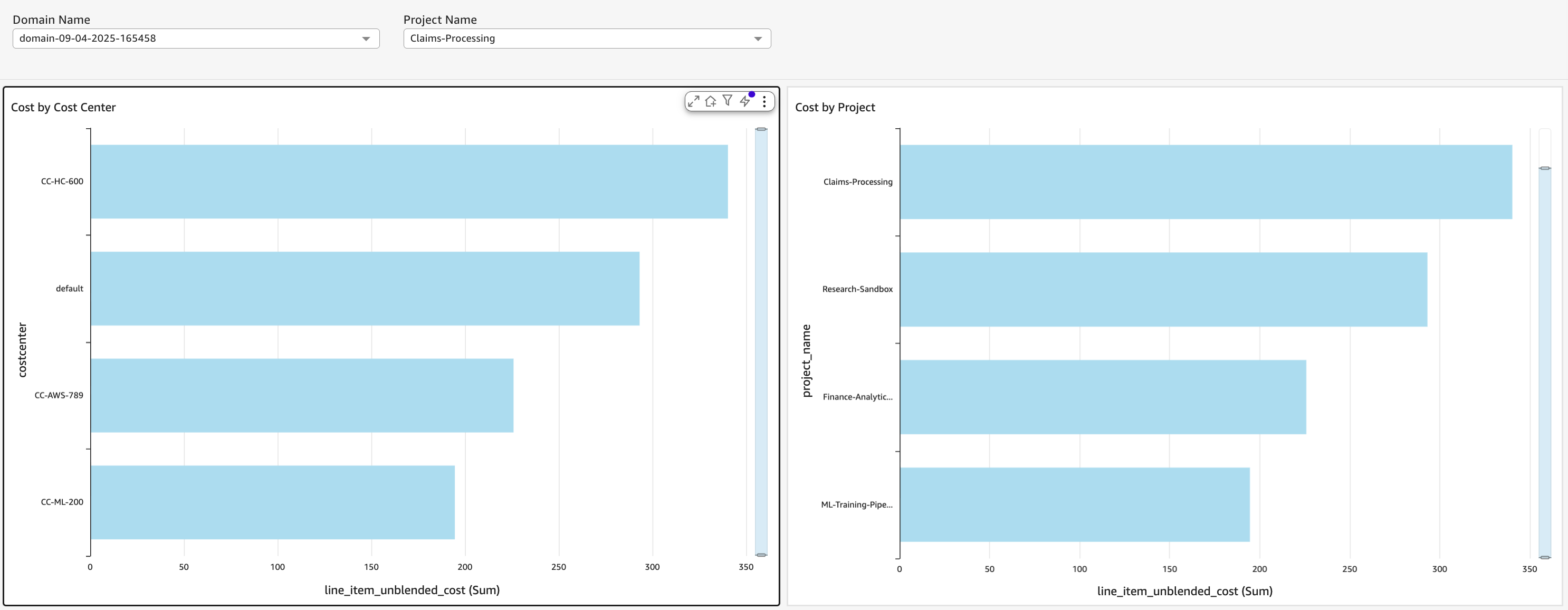
Figure 6: Amazon Quick Sight dashboard showing cost data by custom tags, including Cost by Cost Center and Cost by Project bar charts with Domain Name and Project Name filters
Note: The first end-to-end cycle can take up to 48 hours depending on CUR delivery timing. After the initial cycle completes, subsequent updates will flow automatically on the configured schedule.
Monitoring: The Amazon SNS topic smus-cost-reporting-alerts receives notifications when the AWS Glue ETL job fails or the Lambda orchestrator encounters repeated errors. Subscribe an email address or Slack webhook to stay informed. For instructions on how to create a subscription, see Subscribing to an Amazon SNS topic.
Cost: The solution uses serverless components (Lambda, DynamoDB on-demand, AWS Glue, Amazon Quick Sight, SPICE) so you only pay for what you use. The primary cost drivers are AWS Glue ETL job execution time and Amazon Quick Sight SPICE storage.
Scaling: The DynamoDB table uses on-demand capacity and can scale to accommodate your projects. You can scale the AWS Glue ETL job by increasing the number of workers for larger CUR datasets. For more information, see Managing throughput capacity automatically with DynamoDB auto scaling.
New tag keys: When you add new custom tag keys to projects, the ETL automatically picks them up as new columns. The AWS Glue Crawler’s UPDATE_IN_DATABASE policy adds new columns to the catalog table without manual intervention.
Warning: The following cleanup steps will permanently delete all CUR data, project tag mappings, and Amazon Quick Sight dashboards.
To remove all resources:
Go to AWS Billing and Cost Management, and then choose Data Exports and delete the CUR 2.0 export created in Step 4.
Deactivate the cost allocation tags that were activated in Step 2:
In this post, we showed how to build an end-to-end cost reporting solution for Amazon SageMaker Unified Studio projects using custom tags. This solution combines tag capture driven by Amazon EventBridge, CUR enrichment through AWS Glue ETL, and visualization in Amazon Quick Sight. With it, organizations can track and attribute costs by CostCenter, Team, Environment, or any custom dimension. This works even for resources created through the Studio UI that don’t receive custom tag propagation.
This solution serves as an extension to the custom tag propagation feature and reports cost for all project resources. The architecture is fully serverless, automated, and can be deployed to any AWS account using the provided CDK application.
To start building your custom tag cost reporting pipeline, visit the GitHub repository. To learn more about the underlying services, visit the Amazon SageMaker Unified Studio service page. For a related approach to custom tag governance, see Use Amazon SageMaker custom tags for project resource governance and cost tracking
Post Syndicated from Crosstalk Solutions original https://www.youtube.com/watch?v=1RmAE4lIbDo
Post Syndicated from LastWeekTonight original https://www.youtube.com/watch?v=ciCIrZHUgL4
Post Syndicated from Home Assistant original https://www.youtube.com/shorts/QSLANB46aew
Post Syndicated from jzb original https://lwn.net/Articles/1089721/
Version 26.08 of
the KDE Gear
collection of applications has been released. Notable changes in this release
include improvements in the signing
features of Okular, improved file-grouping
features in the Dolphin file
manager, and a number of enhancements to the Kdenlive video editor. See the changelog for
a full list of updates, enhancements, and bug fixes.
Post Syndicated from corbet original https://lwn.net/Articles/1089720/
The Rust blog reports
on a malicious crate, called proc-macro1, that was uploaded to the
crates.io repository.
Furthermore, we discovered that the popular arrayref crate
had recently been republished and made to depend on this crate,
with the most recent versions yanked. We have removed the malicious
version and unyanked the maliciously-yanked versions. Other crates
by that author (internment, append-only-vec) were
also affected so we have done the same for those, and locked the
account as a precaution. We do not believe the author of
arrayref to be acting maliciously, but their computer or
credentials are likely compromised, and we are attempting to
contact them.
Post Syndicated from jzb original https://lwn.net/Articles/1089719/
Version 6.1.0 of the RPM Package Manager has been released. Notable
changes include the ability to provide modifiers to RPM macros at definition
time, improved build and verification error handling, support for signing files
with PKCS11 tokens using rpmsign, as well as
the addition of several new man pages. The 6.1.0 release also debuts a new release model
inspired by the Linux kernel’s.
Post Syndicated from corbet original https://lwn.net/Articles/1089244/
As of this writing, 2,346 non-merge changesets have been pulled into the
mainline repository for the 7.3 kernel release. That, clearly, is a mere
down payment on the flood that is to come. Even so, those early pulls
brought in some noteworthy changes, including (but not limited to) a
significant reworking of how group scheduling works on multiprocessor
systems.