Introducing Stream Generated Captions, powered by Workers AI

Post Syndicated from Mickie Betz original https://blog.cloudflare.com/stream-automatic-captions-with-ai


With one click, customers can now generate video captions effortlessly using Stream’s newest feature: AI-generated captions for on-demand videos and recordings of live streams. As part of Cloudflare’s mission to help build a better Internet, this feature is available to all Stream customers at no additional cost.

This solution is designed for simplicity, eliminating the need for third-party transcription services and complex workflows. For videos lacking accessibility features like captions, manual transcription can be time-consuming and impractical, especially for large video libraries. Traditionally, it has involved specialized services, sometimes even dedicated teams, to transcribe audio and deliver the text along with video, so it can be displayed during playback. As captions become more widely expected for a variety of reasons, including ethical obligation, legal compliance, and changing audience preferences, we wanted to relieve this burden.

With Stream’s integrated solution, the caption generation process is seamlessly integrated into your existing video management workflow, saving time and resources. Regardless of when you uploaded a video, you can easily add automatic captions to enhance accessibility. Captions can now be generated within the Cloudflare Dashboard or via an API request, all within the familiar and unified Stream platform.

This feature is designed with utmost consideration for privacy and data protection. Unlike other third-party transcription services that may share content with external entities, your data remains securely within Cloudflare’s ecosystem throughout the caption generation process. Cloudflare does not utilize your content for model training purposes. For more information about data protection, review Your Data and Workers AI.

Getting Started

Starting June 20th, 2024, this beta is available for all Stream customers as well as subscribers of the Professional and Business plans, which include 100 minutes of video storage.

To get started, upload a video to Stream (from the Cloudflare Dashboard or via API).

Next, navigate to the “Captions” tab on the video, click “Add Captions,” then select the language and “Generate captions with AI.” Finally, click save and within a few minutes, the new captions will be visible in the captions manager and automatically available in the player, too. Captions can also be generated via the API.

Captions are usually generated in a few minutes. When captions are ready, the Stream player will automatically be updated to offer them to users. The HLS and DASH manifests are also updated so third party players that support text tracks can display them as well.

On-demand videos and recordings of live streams, regardless of when they were created, are supported. While in beta, only English captions can be generated, and videos must be shorter than 2 hours. The quality of the transcription is best on videos with clear speech and minimal background noise.

We’ve been pleased with how well the AI model transcribes different types of content during our tests. That said, there are times when the results aren’t perfect, and another method might work better for some use cases. It’s important to check if the accuracy of the generated captions are right for your needs.

Technical Details

Built using Workers AI

The Stream engineering team built this new feature using Workers AI, allowing us to access the Whisper model – an open source Automatic Speech Recognition model – with a single API call. Using Workers AI radically simplified the AI model deployment, integration, and scaling with an out-of-the-box solution. We eliminated the need for our team to handle infrastructure complexities, enabling us to focus solely on building the automated captions feature.

Writing software that utilizes an AI model can involve several challenges. First, there’s the difficulty of configuring the appropriate hardware infrastructure. AI models require substantial computational resources to run efficiently and require specialized hardware, like GPUs, which can be expensive and complex to manage. There’s also the daunting task of deploying AI models at scale, which involve the complexities of balancing workload distribution, minimizing latency, optimizing throughput, and maintaining high availability. Not only does Workers AI solve the pain of managing underlying infrastructure, it also automatically scales as needed.

Using Workers AI transformed a daunting task into a Worker that transcribes audio files with less than 30 lines of code.

import { Ai } from '@cloudflare/ai'


export interface Env {
 AI: any
}


export type AiVTTOutput = {
 vtt?: string
}


export default {
 async fetch(request: Request, env: Env) {
   const blob = await request.arrayBuffer()


   const ai = new Ai(env.AI)
   const input = {
     audio: [...new Uint8Array(blob)],
   }


   try {
     const response: AiVTTOutput = (await ai.run(
       '@cf/openai/whisper-tiny-en',
       input
     )) as any
     return Response.json({ vtt: response.vtt })
   } catch (e) {
     const errMsg =
       e instanceof Error
         ? `${e.name}\n${e.message}\n${e.stack}`
         : 'unknown error type'
     return new Response(`${errMsg}`, {
       status: 500,
       statusText: 'Internal error',
     })
   }
 },
}

Quickly captioning videos at scale

The Stream team wanted to ensure this feature is fast and performant at scale,   which required engineering work to process a high volume of videos regardless of duration.

First, our team needed to pre-process the audio prior to running AI inference to ensure the input is compatible with Whisper’s input format and requirements.

There is a wide spectrum of variability in video content, from a short grainy video filmed on a phone to a multi-hour high-quality Hollywood-produced movie. Videos may be silent or contain an action-driven cacophony. Also, Stream’s on-demand videos include recordings of live streams which are packaged differently from videos uploaded as whole files. With this variability, the audio inputs are stored in an array of different container formats, with different durations, and different file sizes. We ensured our audio files were properly formatted to be compatible with Whisper’s requirements.

One aspect for pre-processing is ensuring files are a sensible duration for optimized inference.  Whisper has an “sweet spot” of 30 seconds for the duration of audio files for transcription. As they note in this Github discussion: “Too short, and you’d lack surrounding context. You’d cut sentences more often. A lot of sentences would cease to make sense. Too long, and you’ll need larger and larger models to contain the complexity of the meaning you want the model to keep track of.” Fortunately, Stream already splits videos into smaller segments to ensure fast delivery during playback on the web. We wrote functionality to concatenate those small segments into 30-second batches prior to sending to Workers AI.

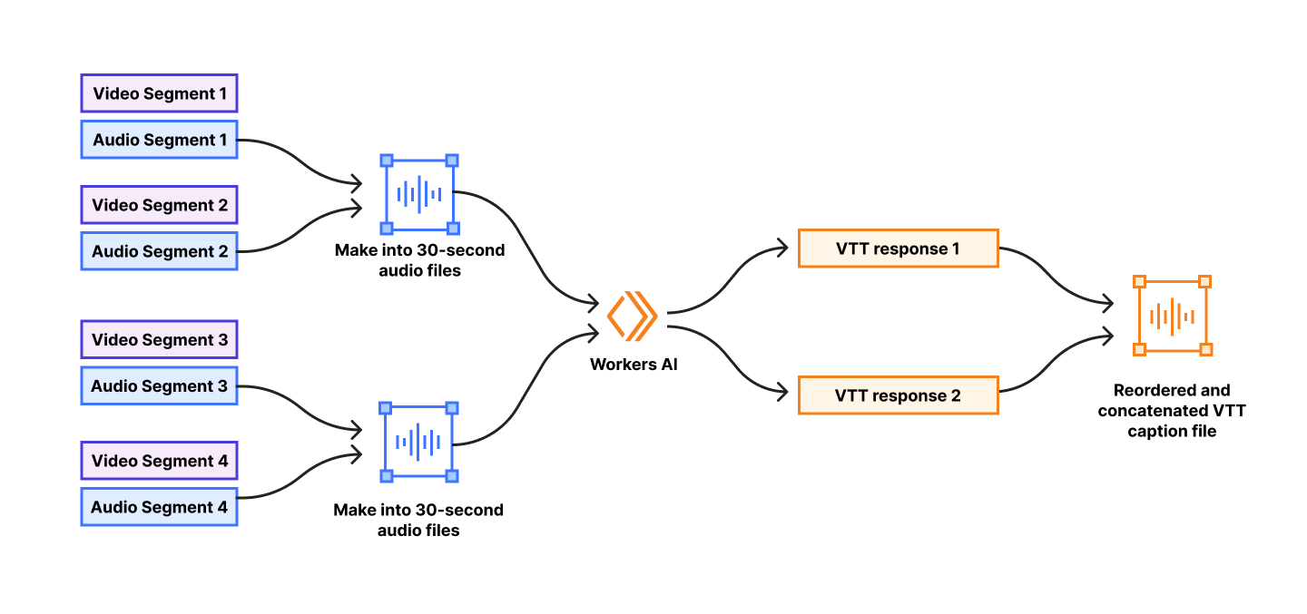
To optimize processing speed, our team parallelized as many operations as possible. By concurrently creating the 30-second audio batches and sending requests to Workers AI, we take full advantage of the scalability of the Workers AI platform. Doing this greatly reduces the time it takes to generate captions, but adds some additional complexity. Because we are sending requests to Workers AI in parallel, transcription responses may arrive out-of-order. For example, if a video is one minute in duration, the request to generate captions for the second 30 seconds of a video may complete before the request for the first 30 seconds of the video. The captions need to be sequential to align with the video, so our team had to maintain an understanding of the audio batch order to ensure our final combined WebVTT caption file is properly synced with the video. We sort the incoming Workers AI responses and re-order timestamps for a final accurate transcript.

The end result is the ability to generate captions for longer videos quickly and efficiently at scale.

Try it now

We are excited to bring this feature to open beta for all of our subscribers as well as Pro and Business plan customers today! Get started by uploading a video to Stream. Review our documentation for tutorials and current beta limitations. Up next, we will be focused on adding more languages and supporting longer videos.

Recovering Public Keys from Signatures

Post Syndicated from Bruce Schneier original https://www.schneier.com/blog/archives/2024/06/recovering-public-keys-from-signatures.html

Interesting summary of various ways to derive the public key from digitally signed files.

Normally, with a signature scheme, you have the public key and want to know whether a given signature is valid. But what if we instead have a message and a signature, assume the signature is valid, and want to know which public key signed it? A rather delightful property if you want to attack anonymity in some proposed “everybody just uses cryptographic signatures for everything” scheme.

Introducing a computing curriculum in Odisha

Post Syndicated from Author original https://www.raspberrypi.org/blog/introducing-a-computing-curriculum-in-odisha/

We are working with two partner organisations in Odisha, India, to develop and roll out the IT & Coding Curriculum (Kaushali), a computing curriculum for government high schools. Last year we launched the first part of the curriculum and rolled out teacher training. Read on to find out what we have learned from this work.

A group of teachers is standing outside a school building.

Supporting government schools in Odisha to teach computing

Previously we shared an insight into how we established Code Clubs in Odisha to bring computing education to young people. Now we are partnering with two Indian civil society organisations to develop high school curriculum resources for computing and support teachers to deliver this content.

With our two partners, we trained 311 master teachers during July and August 2023. The master teachers, most often mathematics or science teachers, were in turn tasked with training teachers from around 8000 government schools. The aim of the training was to enable the 8000 teachers to deliver the curriculum to grades 9 and 10 in the June 2023 – April 2024 academic year.

A master teacher is delivering a training session to a group of teachers.

At the Foundation, we have been responsible for providing ongoing support to 1898 teachers from 10 districts throughout the academic year, including through webinars and other online and in-person support.

To evaluate the impact our work in Odisha is having, we gathered data using a mixed-methods approach that included gathering feedback from teachers via surveys and interviews, visiting schools, capturing reflections from our trainers, and reviewing a sample of students’ projects.

Positive impact on teachers and students

In our teacher survey, respondents were generally positive about the curriculum resources:

  • 87% of the 385 respondents agreed that the curriculum resources were both high quality and useful for their teaching
  • 91% agreed that they felt more confident to teach students IT & Coding as a result of the curriculum resources

Teachers also tended to agree that the initial training had helped improve their understanding and confidence, and they appreciated our ongoing support webinars.

“The curriculum resources are very useful for students.” – Teacher in Odisha

“The webinar is very useful to acquire practical knowledge regarding the specific topics.”  – Teacher in Odisha

Teachers who responded to our survey observed a positive impact on students:

  • 93% agreed their students’ digital literacy skills had improved
  • 90% agreed that their students’ coding knowledge had improved

Students’ skills were also demonstrated by the Scratch projects we reviewed. And students from Odisha shared 314 projects in Coolest Projects — our online technology showcase for young people — including the project ‘We’ll build a new Odisha’ and an apple catching game.

A master teacher is delivering a training session to a group of teachers.

Feedback and observations about teacher training

On school visits, our team observed that the teachers adopted and implemented the practical elements of the initial training quite well. However, survey responses and interviews showed that often teachers were not yet using all the elements of the curriculum as intended.

In their feedback, many teachers expressed a need for further regular training and support, and some reported additional challenges, such as other demands on their time and access to equipment.

A master teacher is delivering a training session to a group of teachers.

When we observed training sessions master teachers delivered to teachers, we saw that, in some cases, information was lost within the training cascade (from our trainers, to master teachers, to teachers), including details about the intended pedagogical approach. It can be difficult to introduce experienced teachers to new pedagogical methods within a short training session, and teachers’ lack of computing knowledge also presents a challenge.

We will use all this data to shape how we support teachers going forward. Some teachers didn’t share feedback, and so in our further evaluation work, we will focus on making sure we hear a broad and representative range of teachers’ views and experiences.

What’s new this year?

In the current academic year, we are rolling out more advanced curriculum content for grade 10 students, including AI literacy resources developed at the Foundation. We’re currently training master teachers on this content, and they will pass on their knowledge to other teachers in the coming months. Based on teachers’ feedback, the grade 10 curriculum and the training also include a recap of some key points from the grade 9 curriculum.

Two master teachers are delivering a presentation to teachers.

A State Resource Group (SRG) has also been set up, consisting of 30 teachers who will support us with planning and providing ongoing support to master teachers and other teachers in Odisha. We have already trained the SRG members on the new curriculum content to enable them to best support teachers across the state. In addition to this, our local team in Odisha plans to conduct more visits and reach out directly to teachers more often. 

Our plans for the future

The long-term vision for our work in India is to enable any school in India to teach students about computing and creating with digital technologies. A critical part of achieving this vision is the development of a comprehensive computing curriculum for grade 6 to 12, specifically tailored for government schools in India. Thanks to our work in Odisha, we are in a better position to understand the unique challenges and limitations of government schools. We’re designing our curriculum to address these challenges and ensure that every Indian student has the opportunity to thrive in the 21st century. If you would like to know more about our work and impact in India, please reach out to us via [email protected].

We take evaluation of our work seriously and are always looking to understand how we can improve and increase the impact we have on the lives of young people. To find out more about our approach to impact, you can read about our recently updated theory of change, which supports how we evaluate what we do.

The post Introducing a computing curriculum in Odisha appeared first on Raspberry Pi Foundation.

Слуховете за смъртта на американската мечта са силно преувеличени

Post Syndicated from Александър Детев original https://www.toest.bg/sluhovete-za-smurtta-na-amerikanskata-mechta-sa-silno-preuvelicheni/

Слуховете за смъртта на американската мечта са силно преувеличени

Часът е 19:10 и температурата на въздуха е близо 30 градуса. Въпреки това упорито стоя на верандата, преди да потеглим за вечеря, а не в климатизираната къща. Защо? Ами защото съм в Америка и къщата, където спя, има предна веранда – точно като тези, които съм гледал стотици пъти по филмите и за които съм чел в още десетки книги. 

Отляво съседите обсъждат омара, който са купили и трябва да сготвят, докато котката Лесли се катери по парапета, после пада от него и набързо бива прибрана вътре. Отдясно майката явно приключва работния ден, затваря лаптопа и привиква мъжа си и сина си от съседите, за да сядат да вечерят. 

Всичко наоколо продължава да ми се струва сюрреалистично, въпреки че вече сме тук от два дни. Ако кажа още веднъж, че нещо е „като по филмите“, приятелите ми вероятно ще спрат да се забавляват с тази тъпа фраза и ще вземат бейзболната бухалка… като по филмите. 

Вашингтон

Америка е такава, каквото си я представях. Дори столицата Вашингтон, която, както ще се убедя по-късно, е всичко друго, но не и типичният американски град. Обликът, атмосферата, външният вид и облеклото на хората могат да се сменят през две преки. От съседите ни, които толкова се вписват в стереотипа за живеещата „мечтата“ средна класа, че чак е банално, до отрупания с боклуци паркинг на няколко преки от къщата ни, където виждаш онези развалени зъби, петна по кожата и неадекватно поведение, които недвусмислено ти говорят за проблема с наркотиците в САЩ, ставащ все по-драматичен с всяка изминала година. 

Но да погледнем малко по-ведро. „Добре че сте дошли първо на Източния бряг, защото вие в Европа сте свикнали да се разхождате“, ми казва Кайл*, с когото се запознаваме в един бар същата тази вечер. Американец, който знае къде е Пловдив. Да, не се шегувам! Бил в Гърция и оттогава му станало любопитно, затова четял за Балканите. 

Стереотипите са тъпи. Мисля, че съм напълно убеден в това, но с всяко следващо пътуване се убеждавам все повече. И все пак между Европа и САЩ има разлики. Дори между Европа и доста европейски изглеждащия Вашингтон. 

Да започнем с цените. „Едно от най-неудобните неща тук е, че цената, която виждаш в менюто, не отговаря на финалната“, обяснява Младен Петков, български журналист, който от години живее и работи в САЩ. Да вземем например една бира. Според менюто или дъската, закачена над бара, тя струва 9 долара. Скъпо, но поносимо. Само че в сметката ти далеч не е толкова. Първо добавяш данъка, който не е калкулиран, след това слагаш и задължителния или незаобиколимо препоръчителния бакшиш, който в последните години е 18, 20 или дори 22%. И така цената на една бира в заведение в САЩ задминава драстично и най-скъпите европейски градове, като Лондон, Стокхолм и Созопол**. Темата за храната изобщо няма да я повдигам – фастфуд или плащаш със затворени очи. 

Вашингтон няма някакви емблематични ястия, но предвид размера и статута му това е по-скоро обяснимо. Столицата на най-великата сила в света всъщност изобщо не е голям град. Целият център се обхожда пеша, задръстванията са само в час пик, и то напълно приемливи, а вечер в делничен ден навън няма особено много хора. 

Като говорим за емблематични ястия обаче, е време да се насочим към следващата точка – дома на чийзстейка – Филаделфия, щата Пенсилвания. И съвсем закономерно барманката във Вашингтон се оказва именно оттам. „Как се разбирате изобщо в Пенсилвания?“, питам я аз. Все пак това е един от най-разделените щати, един от тези, които определят изхода от изборите в последните години. „Ами хората, които живеем в града, и тези, които живеят в селата, сме много различни – обяснява тя. – И сме си свикнали така. Иначе аз не се притеснявам за ноември – живели сме го веднъж, ще го преживеем пак.“

И в този момент за последен път някой ми спомена Тръмп по време на пътуването ни. Хората по крайбрежията предпочитат да го игнорират. Явно защото „веднъж са го живели, ще го преживеят пак“. 

Филаделфия

„Във Филаделфия винаги е слънчево“, гласи заглавието на онзи безсрамно неполиткоректен, но и неприлично смешен сериал. И наистина, слънцето на 4 юни го доказва. Термометрите показват над 30 градуса. Чао, Вашингтон, здравей, Америка! 

Филаделфия представлява амалгама от стари небостъргачи, чисто нови небостъргачи, квартали с ниски къщички, графити, симпатични веранди и гета, в които е силно препоръчително да не стъпваш, както ни информира таксиметровият шофьор, при когото се качваме от гарата. Той е от Таджикистан, тук е от две години. Какво може да препоръча във Фили? „Ами то тук няма много неща за правене, само работа, работа, работа.“ 

30 минути по-късно: абсолютен контраст. Запознаваме се с Джейми и Шарън, които пият бира на рууфтоп бара на сградата, в която сме отседнали. Тя живее в Ирландия, но се е прибрала в родната Пенсилвания за няколко седмици. „Ама защо сте само един ден тук, няма да ви стигне изобщо! Фили е супер, ей сега ще ви кажем къде да отидете.“ Два свята – една мечта. 

Фили не само ти разказва историята на САЩ от генезиса на американската държава и краткия период, в който градът е бил столица, но ти я и показва – през улиците, за които пее и Брус Спрингстийн, и през усещането, че този симпатичен и цветен град в същото време е далеч от своя зенит и от прогреса, на който се е радвал преди десетилетия.

Ню Йорк 

И тъй като споменах истории – следващата ни дестинация е вдъхновила повече истории от всяка друга. Start spreading the news, взимаме автобуса и потегляме към Empire State of Mind

Какво има неказано за Ню Йорк? И как да опиша динамиката и необятността му по-добре от Били Джоел, Франк Синатра и Нас? Трудно, затова нека опитаме с един маршрут за разходка: слезте от влака или от автобуса сред тълпите в Централен Манхатън, вземете си метрото до Чайнатаун, минавайки през няколкото останали улици на Малката Италия. Оттам тръгнете по Уолстрийт и се разходете пеша до пристанището, от което потеглят корабчетата за Статуята на Свободата. След като акостирате обратно, минете пеша по Бруклинския мост и си вземете метрото, за да отидете да поплажувате на Кони Айлънд. 

Ню Йорк не е град, Ню Йорк е свят. И в този свят блясъкът на небостъргачите и умовете съжителства със сенките на престъпността и плъховете по улиците. 

Ню Йорк е град, в който всеки си е на мястото, но никой не е у дома. Освен Фран Лебовиц, разбира се. С всяка изминала година Голямата ябълка става все по-скъпа и по-населена, а свързването на двата края – все по-сериозно предизвикателство. Но това не спира хора от цялата страна и от всяка точка на земното кълбо да пристигат тук, решени да успеят. Защото ако успеят тук, ще успеят навсякъде, както ни напомнят Алиша Кийс и Джей Зи

Сред тях са също Кирим от Лондон и Матрик, който е в Ню Йорк заедно с майка си Ема. Матрик свири на чело, и то виртуозно. Кирим пък е брилянтен пианист. Срещаме ги в Сентръл парк, където Матрик изпълнява всяка музикална поръчка – от Бритни Спиърс до „Лед Цепелин“. Кирим си търси пиано. Чувал е, че някакъв човек обикаля с пиано на колела из парка, но още не го е срещал. Докато не го срещне, можем да се наслаждаваме на творчеството му само в социалните мрежи. Или когато му отидем на гости в Лондон. Но засега тримата остават в Сентръл парк, заобиколени от случайни минувачи, катерички и врабчета, които щъкат и прелитат наоколо, и миризма на джойнт и свобода във въздуха. 

Само на няколко метра оттук са едни от най-големите и емблематични сцени в света. Да, за Бродуей става въпрос. Лин-Мануел Миранда е създал помоему първия пост-Андрю Лойд Уебър мюзикъл – „Хамилтън“ няма нищо общо с класическите мюзикъли на Бродуей, нито пък с начина, по който сме свикнали да бъде разказвана историята на САЩ. Но има много общо с една от най-важните спойки на обществото тук, градяща мостове между различни хора, общности и етноси – музиката. В „Хамилтън“ тя е толкова великолепна, хореографията – толкова безупречна, а диалозите така балансирани между фактите и хумора, че не отделяш очи и уши от сцената в продължение на два часа и половина. 

След като видиш мюзикъл на Бродуей, няма как да пропуснеш и друг стожер на поп културата – вечерната (late night) телевизия. Американската телевизия не е като европейската. Знам, че не откривам топлата вода, но заснемането на едночасово шоу за час и двайсет минути с такъв синхрон между седемте камери, операторите, публиката и стейдждиректора е впечатляващо. А Стивън Колбер е точно такъв пич извън ефир, какъвто е и на екрана. Да живее Стивън, да живее Late Show, да живее и театър „Ед Съливан“! 

Ню Йорк едновременно те зарежда както никой друг град и те изморява както никое друго място на планетата. Ню Йорк се преживява, не се разказва. Затова спирам дотук. И ви прехвърлям на север към държавата, от която Ниагарските водопади се виждат по-добре. 

Торонто

Торонто е симпатичен град, но бледнее пред Ню Йорк. 

(Дали не съм обречен да казвам това за всеки град, който посетя занапред?)

Иначе разликата между САЩ и Канада в динамиката на живота, усещането за сигурност и спокойствие, както и в цените е голяма. А и стереотипът е верен (въпреки че стереотипите по принцип са тъпи, както вече споменах) – канадците наистина са изключително отзивчиви и мили. И как да не са – един от най-високите стандарти на живот, безплатно здравеопазване и изключително ниско ниво на престъпност, особено в сравнение със Съединените щати. 

„Живея в Канада, защото съм по-лява“, казва Ели, дошла тук преди 31 години. Гостува ѝ нейната приятелка Лили, която живее в Калифорния – „едно от малкото места в САЩ, където има вкусни зеленчуци“. Двете приятелки са завършили заедно във Враца, а в началото на 90-те успяват да емигрират в Канада по точкова система.

Сега се срещат в Торонто, за да отидат заедно на българския фестивал „Фолклорен водопад“, който се провежда на Ниагара. „Не показност, демонстрация или фалшив патриотизъм, а истинска любов към българския фолклор, приятелите и Родината“, написаха през 2023-та организаторите. Не фалшив патриотизъм, а точно любов към родината блести в погледа на българите в чужбина, когато говорят за спорадичните си прибирания в България. 

Иначе Канада си е една леко вълшебна държава, в която животът си върви по свой чак дебилно спокоен и оптимистичен начин. Дори когато хората се натъкват на трудности.

Историята на Тери Фокс го доказва. „Извинявайте, че няма да мога да продължа да тичам“, казва той само месеци преди кончината си през 1981 г. Тери се сблъсква с диагнозата рак през 1977 г., когато е само на 19. Скоро губи и крака си. Ракът обаче не го спира да се изправи и да изтича 5373 километра с протеза, за да събере пари за борбата с онкологичните заболявания. Той тича 143 дни, преди коварната болест да го спре и впоследствие да отнеме живота му едва на 22. В последното си публично изказване, типично по канадски, Тери Фокс се извинява, че няма да може да продължи да извършва нечовешките си подвизи. В тази вълшебна по свой си начин държава всички се извиняват. И живеят добре. 

Бостън

Жителите на Масачузетс, от друга страна, имат славата на едни от най-грубите американци. На посетителите от Източна Европа ни е малко трудно да го забележим, честно казано, а и в средата на юни властва такава еуфория покрай мача на „Селтикс“, че място за негативни емоции няма. Масачузетс, подобно на Мейн и повечето щати по Североизточното крайбрежие, е известен със своята морска кухня и по-конкретно с омарите. Така нареченият lobster roll е най-популярната бърза храна в Бостън и околията от десетилетия. 

Приятелка, която е учила в първия град на САЩ, ми препоръчва къде да пробваме прословутите сандвичи. По нейно време – тоест преди има-няма 10 години – той е струвал 8 долара. Днес е… 40. Пък едно време затворниците в Бостън са протестирали, защото са ги хранили само с омари, „тези огромни хлебарки от океана“, както ги нарича Джеремая. Той е гид в един от най-старите градове в САЩ. 

От него научаваме повече и за прословутото преследване на вещици в Сейлъм през XVII век. Покрай няколкостотин невинни жени, пострадали от поредната човешка лудост, са си заминали и две кучета, които също са били обвинени и осъдени за вещерство. 37 котки също са били обвинени, но след това са оправдани… Че кой би се отварял на котка? 

И така в шеги и закачки нашето пътуване върви към своя край. Америка днес е изправена пред много трудности и предизвикателства, но слуховете за смъртта на американската мечта са силно преувеличени. Емпайър Стейт Билдинг все така блести отвисоко, а хората вярват в по-доброто утре.


* Поради вродена невъзможност за запомняне на имена и високоалкохолните бири, които консумират в САЩ, някои имена в този разказ са налучквани, тъй като авторът е забравил истинските. 

** Алтернативното заглавие на този текст беше „Почти като Созопол, ама малко по-скъпо“. Следващ пътепис – Созопол!

Палеогеномиката и тайните на античната ДНК

Post Syndicated from original https://www.toest.bg/paleogenomikata-i-taynite-na-antichnata-dnk/

Палеогеномиката и тайните на античната ДНК

Усъвършенстването на методите за извличане и разчитане на ДНК от фосилни останки е голям пробив в областта на еволюционната генетика. Новите открития дават повече яснота за произхода на човешката популация, за историческия поглед върху миграционните движения и степента на смесване между хората и античните, вече изчезнали Hominini¹, като неандерталците, както и между съвременните човешки популации. 

Палеогеномиката излиза от границите на антропологията и се очаква да даде отговор на множествено неизяснени въпроси с ключово значение в съвременната медицина.

Тя ни предлага поглед към човешкото здраве през различни периоди, разкривайки включително и наличието на предишни епидемии. Тези научни изследвания позволяват да обогатим знанията си за връзката между настоящото генетично разнообразие и болестите; да изясним генетичните основи на съвременните заболявания, в това число и вродени грешки на имунитета, които пречат на адекватния отговор на инфекции; да разработим нови лекарства и терапии. 

Палеогеномиката като машина на времето

Палеогеномиката е наука за реконструирането и анализа на геномите на организми, които вече не съществуват. Тези анализи могат да предоставят информация кога и как са се изменили определени характеристики на даден вид и как изчезналите видове са свързани с живите в настоящето организми и популации. 

Това е сравнително нова научна област, която не би могла да съществува без напредъка в технологиите за възстановяване на антична ДНК (аДНК) от запазени останки, както и без анализа на аДНК с подходи като секвениране от ново поколение и реконструиране на целия геном чрез правилното подреждане на множеството къси, често увредени фрагменти от аДНК. Палеогеномните анализи може да се възприемат като добавка към съвременните изследвания, фокусирани върху човешката физиология. Чрез проучването на части от човешкия геном с установени примеси от неандерталски материал се откриват гени с важно физиологично значение. 

Приносите на палеогеномиката обаче не свършват с това. С нарастващия брой аДНК проби става възможен отговорът на множество въпроси, свързани с човешкото здраве – например как човечеството е успяло да оцелее след излагането на патогени в миналото.

На базата на изследвания на модерния човек е известно, че определени мутации в ДНК променят механизмите ни за защита от патогени, което от своя страна обяснява защо са налице най-разнообразни реакции на дадена инфекция. От фосилни останки могат да се изследват промените в честотата на дадени генетични варианти, които влияят върху риска от развитие на инфекциозни заболявания. Това е, един вид, постоянен и безсрочен експеримент с ясно доказателство за стойността на палеогеномиката в медицината.

Първият пълен човешки палеогеном

Най-старият изследван геном от род Homo е от останки на неандерталец на приблизителна възраст 430 000 години, а най-новите налични антични геноми са на не повече от 10 000 години. Античната ДНК е извлечена от проби по целия свят, предимно от северното полукълбо, поради което в геномните изследвания са включени основно останки от европейски предшественици на съвременните хора.

През 2010 г. екипът на Rasmussen публикува данни от първия човешки палеогеном, извлечен от изключително добре запазена проба от коса на палеоескимос. Учените успяват да възстановят 79% от генома и да затвърдят връзката между палеоескимосите и настоящите човешки популации чрез сравняване на митохондриалния геном. Геномът, получен от тази проба, издава също, че собственикът му е с кръвна група А+, че очите му са били кафяви (носител е на вариант в HERC2-OCA2 региона², свързан с този цвят на очите), както и че е бил добре адаптиран към студения климат (на базата на генетични варианти, имащи връзка с метаболизма).

Античната ДНК и съвременните проблеми с нейното анализиране

Античната ДНК е изложена на редица неблагоприятни фактори на околната среда. В резултат тя се разгражда и не може да оцелее повече от един милион години дори и в идеални условия, като ниски температури и ниска влажност. Голяма част от наличната днес аДНК е извлечена от перманентно замразена среда (например арктически лед). 

Друг проблем, който затруднява анализирането на аДНК, е контаминацията с друга ДНК. аДНК често може да се открие в почви заедно с други източници на ДНК, като растения, гъби и бактерии. Например първият неандерталски палеогеном съдържа само 5% истинска неандерталска ДНК. При най-успешните опити за извличане на аДНК тя варира между 70 и 95%. 

Друг източник на замърсяване с външна ДНК би могъл да бъде начинът на съхраняване и обработка на аДНК.

Най-голямото предизвикателство пред успешния анализ на аДНК е разграничаването ѝ от външната ДНК, независимо от източника ѝ. Заради тези трудности в началото са направени грешки, които сега се преодоляват със следването на протоколи за работа, специално разработени за анализ на аДНК в специализирана стерилна работна среда.

Палеогеномика и медицина – настояще и бъдеще

С увеличаването на пробите с висококачествена аДНК се увеличават и очакванията за приноса на палеогеномиката в медицинските научни изследвания. Но тук възниква следващата пречка, а именно т.нар. плейотропия – когато един и същ ген е отговорен за различни фенотипни изяви).

Изследване на повече от 2000 антични европейски генома сочи, че през последните хилядолетия са естествено селектирани генетични варианти, отговорни за промени при риска от инфекция и едновременно с това свързани с автоимунни прояви. 

Преобладаващите генетични варианти, свързани с риск от развитие на автоимунитет, най-вероятно са резултат от позитивна селекция след взаимодействието с патогени от околната среда, тъй като тези варианти отговарят и за понижаване на риска от протичане на инфекциозно заболяване. 

Позитивният селективен натиск настъпва поради естествения подбор на определени генетични варианти. Вследствие на отговор на фактори от околната среда честотата на даден генетичен вариант се увеличава в популацията. Пример за такъв естествен селективен натиск е защитата от развитие на маларийна инфекция при хора със сърповидноклетъчна анемия. Маларията е най-разпространена в Африка, където е повишена и честотата на хора, носители на едно здраво копие и едно мутантно копие за гена, произвеждащ хемоглобин. Паразитите, които маларийният комар пренася, инфектират червените кръвни клетки, но при сърповидноклетъчна анемия те са с променена структура и не могат да пренасят кислород. Паразитът се развива по-бавно в тази среда и дава време на имунната система да реагира и да го унищожи.

Откритието на такива плейотропни варианти с помощта на палеогеномиката би могло да спомогне за разработването на лекарства с по-малко странични ефекти. Анализът на чревни микробиоми от древността също може да даде информация как да се справим с антибиотичната резистентност, като изследва еволюцията и разпространението ѝ. Еволюцията на човешкия имунитет също може да се изследва с помощта на антични протеини като антитела и през взаимодействието им с патогените.

1 Hominini са член на подсемейството Homininae, което включва видове от рода Homo, като модерния човек (Homo sapiens), Неандерталеца (Homo neanderthalensis) и Денисовия човек (Denisova hominin).
2 HERC2 е доста голям ген, локализиран на дългото рамо на 15-тата хромозома (локализация: 15q13). Той може да потиска експресията на гена OCA2, който също е локализиран на дългото рамо на същата хромозома (локализация: 15q13.1).
OCA2 е отговорен за продукцията на меланин в ириса. Мутации в HERC2, който е съседен на OCA2, оказват влияние върху експресията на OCA2 и резултатът е сини очи при хората. Нарича се „HERC2-OCA2 регион“, защото тези гени са точно един до друг и са свързани с пигментацията.

New Blog Moderation Policy

Post Syndicated from Bruce Schneier original https://www.schneier.com/blog/archives/2024/06/new-blog-moderation-policy.html

There has been a lot of toxicity in the comments section of this blog. Recently, we’re having to delete more and more comments. Not just spam and off-topic comments, but also sniping and personal attacks. It’s gotten so bad that I need to do something.

My options are limited because I’m just one person, and this website is free, ad-free, and anonymous. I pay for a part-time moderator out of pocket; he isn’t able to constantly monitor comments. And I’m unwilling to require verified accounts.

So starting now, we will be pre-screening comments and letting through only those that 1) are on topic, 2) contribute to the discussion, and 3) don’t attack or insult anyone. The standard is not going to be “well, I guess this doesn’t technically quite break a rule,” but “is this actually contributing.”

Obviously, this is a subjective standard; sometimes good comments will accidentally get thrown out. And the delayed nature of the screening will result in less conversation and more disjointed comments. Those are costs, and they’re significant ones. But something has to be done, and I would like to try this before turning off all comments.

I am going to disable comments on the weekly squid posts. Topicality is too murky on an open thread, and these posts are especially hard to keep on top of.

Comments will be reviewed and published when possible, usually in the morning and evening. Sometimes it will take longer. Again, the moderator is part time, so please be patient.

I apologize to all those who have just kept commenting reasonably all along. But I’ve received three e-mails in the past couple of months about people who have given up on comments because of the toxicity.

So let’s see if this works. I’ve been able to maintain an anonymous comment section on this blog for almost twenty years. It’s kind of astounding that it’s worked as long as it has. Maybe its time is up.

[$] How free software hijacked Philip Hazel’s life

Post Syndicated from jzb original https://lwn.net/Articles/978463/

Philip Hazel was 51 when he began the Exim message transfer agent (MTA)
project in 1995, which
led to the Perl-Compatible Regular
Expressions
(PRCE) project in 1998. At 80,
he’s maintained PCRE, and its successor PCRE2, for more than 27
years. For those doing the math, that’s a year longer than LWN has
been in publication. Exim maintenance was handed off around the time
of his retirement in 2007. Now, he is ready to hand off PCRE2 as well,
if a successor can be found.

Blue/Green Deployments to Amazon ECS using AWS CloudFormation and AWS CodeDeploy

Post Syndicated from Ajay Mehta original https://aws.amazon.com/blogs/devops/blue-green-deployments-to-amazon-ecs-using-aws-cloudformation-and-aws-codedeploy/

Introduction

Many customers use Amazon Elastic Container Service (ECS) for running their mission critical container-based applications on AWS. These customers are looking for safe deployment of application and infrastructure changes with minimal downtime, leveraging AWS CodeDeploy and AWS CloudFormation. AWS CloudFormation natively supports performing Blue/Green deployments on ECS using a CodeDeploy Blue/Green hook, but this feature comes with some additional considerations that are outlined here; one of them is the inability to use CloudFormation nested stacks, and another is the inability to update application and infrastructure changes in a single deployment. For these reasons, some customers may not be able to use the CloudFormation-based Blue/Green deployment capability for ECS. Additionally, some customers require more control over their Blue/Green deployment process and would therefore like CodeDeploy-based deployments to be performed outside of CloudFormation.

In this post, we will show you how to address these challenges by leveraging AWS CodeBuild and AWS CodePipeline to automate the configuration of CodeDeploy for performing Blue/Green deployments on ECS. We will also show how you can deploy both infrastructure and application changes through a single CodePipeline for your applications running on ECS.

The solution presented in this post is appropriate if you are using CloudFormation for your application infrastructure deployment. For AWS CDK applications, please refer to this post that walks through how you can enable Blue/Green deployments on ECS using CDK pipelines.

Reference Architecture

The diagram below shows a reference CICD pipeline for orchestrating a Blue/Green deployment for an ECS application. In this reference architecture, we assume that you are deploying both infrastructure and application changes through the same pipeline.

CICD Pipeline for performing Blue/Green deployment to an application running on ECS Fargate

Figure 1: CICD Pipeline for performing Blue/Green deployment to an application running on ECS Fargate Cluster

The pipeline consists of the following stages:

  1. Source: In the source stage, CodePipeline pulls the code from the source repository, such as AWS CodeCommit or GitHub, and stages the changes in S3.
  2. Build: In the build stage, you use CodeBuild to package CloudFormation templates, perform static analysis for the application code as well as the application infrastructure templates, run unit tests, build the application code, and generate and publish the application container image to ECR. These steps can be performed using a series of CodeBuild steps as described in the reference pipeline above.
  3. Deploy Infrastructure: In the deploy stage, you leverage CodePipeline’s CloudFormation deploy action to deploy or update the application infrastructure. In this stage, the entire application infrastructure is set up using CloudFormation nested stacks. This includes the components required to perform Blue/Green deployments on ECS using CodeDeploy, such as the ECS Cluster, ECS Service, Task definition, Application Load Balancer (ALB) listeners, target groups, CodeDeploy application, deployment group, and others.
  4. Deploy Application: In the deploy application stage, you use the CodePipeline ECS-to-CodeDeploy action to deploy your application changes using CodeDeploy’s blue/green deployment capability. By leveraging CodeDeploy, you can automate the blue/green deployment workflow for your applications running on ECS, including testing of your application after deployment and automated rollbacks in case of failed deployments. CodeDeploy also offers different ways to switch traffic for your application during a blue/green deployment by supporting Linear, Canary, and All-at-once traffic shifting options. More information on CodeDeploy’s Blue/Green deployment workflow for ECS can be found here

Considerations

Some considerations that you may need to account for when implementing the above reference pipeline

1. Creating the CodeDeploy deployment group using CloudFormation
For performing Blue/Green deployments using CodeDeploy on ECS, CloudFormation currently does not support creating the CodeDeploy components directly as these components are created and managed by CloudFormation through the AWS::CodeDeploy::BlueGreen hook. To work around this, you can leverage a CloudFormation custom resource implemented through an AWS Lambda function, to create the CodeDeploy Deployment group with the required configuration. A reference implementation of a CloudFormation custom resource lambda can be found in our solution’s reference implementation here.

2. Generating the required code deploy artifacts (appspec.yml and taskdef.json)
For leveraging the CodeDeployToECS action in CodePipeline, there are two input files (appspec.yml and taskdef.json) that are needed. These files/artifacts are used by CodePipeline to create a CodeDeploy deployment that performs Blue/Green deployment on your ECS cluster. The AppSpec file specifies an Amazon ECS task definition for the deployment, a container name and port mapping used to route traffic, and the Lambda functions that run after deployment lifecycle hooks. The container name must be a container in your Amazon ECS task definition. For more information on these, see Working with application revisions for CodeDeploy. The taskdef.json is used by CodePipeline to dynamically generate a new revision of the task definition with the updated application container image in ECR. This is an optional capability supported by the CodeDeployToECS action where it can automatically replace a place holder value (for example IMAGE1_NAME) for ImageUri in the taskdef.json with the Uri of the updated container Image. In the reference solution we do not use this capability as our taskdef.json contains the latest ImageUri that we plan to deploy. To create this taskdef.json, you can leverage CodeBuild to dynamically build the taskdef.json from the latest task definition ARN. Below are sample CodeBuild buildspec commands that creates the taskdef.json from ECS task definition

build:
    commands:
        # Create appspec.yml for CodeDeploy deployment
        - python iac/code-deploy/scripts/update-appspec.py --taskArn ${TASKDEF_ARN} --hooksLambdaArn ${HOOKS_LAMBDA_ARN} --inputAppSpecFile 'iac/code-deploy/appspec.yml' --outputAppSpecFile '/tmp/appspec.yml'
        # Create taskdefinition for CodeDeploy deployment
        - aws ecs describe-task-definition --task-definition ${TASKDEF_ARN} --region ${AWS_REGION} --query taskDefinition >> taskdef.json
    artifacts:
        files:
            - /tmp/appspec.yml
            - /tmp/taskdef.json
        discard-paths: yes

To generate the appspec.yml, you can leverage a python or shell script and a placeholder appspec.yml in your source repository to dynamically generate the updated appspec.yml file. For example, the below code snippet updates the placeholder values in an appspec.yml to generate an updated appspec.yml that is used in the deploy stage. In this example, we set the values of AfterAllowTestTraffic hook, the Container name, Container port values from task definition and Hooks Lambda ARN that is passed as input to the script.


  contents = yaml.safe_load(file)
  print(contents)
  response = ecs.describe_task_definition(taskDefinition=taskArn)
  contents['Hooks'][0]['AfterAllowTestTraffic'] = hooksLambdaArn
  contents['Resources'][0]['TargetService']['Properties']['LoadBalancerInfo']['ContainerName'] = response['taskDefinition']['containerDefinitions'][0]['name']
  contents['Resources'][0]['TargetService']['Properties']['LoadBalancerInfo']['ContainerPort'] = response['taskDefinition']['containerDefinitions'][0]['portMappings'][0]['containerPort']
  contents['Resources'][0]['TargetService']['Properties']['TaskDefinition'] = taskArn

  print('Updated appspec.yaml contents')
  yaml.dump(contents, outputFile)

In the above scenario, the existing task definition is used to build the appspec.yml. You can also specify one of more CodeDeploy lambda based hooks in the appspec.yml to perform variety of automated tests as part of your deployment.

3. Updates to the ECS task definition
To perform Blue/Green deployments on your ECS cluster using CodeDeploy, the deployment controller on the ECS Service needs to be set to CodeDeploy. With this configuration, any time there is an update to the task definition on the ECS service (such as when building new application image), the update results in a failure. This essentially causes CloudFormation updates to the application infrastructure to fail when new application changes are deployed. To avoid this, you can implement a CloudFormation based custom resource that obtains the previous version of task definition. This prevents CloudFormation from updating the ECS Service with new task definition when the application container image is updated and ultimately from failing the stack update. Updates to ECS Services for new task revisions are performed using the CodeDeploy deployment as outlined in #2 above. Using this mechanism, you can update the application infrastructure along with changes to the application code using a single pipeline while also leveraging CodeDeploy Blue/Green deployment.

4. Passing configuration between different stages of the pipeline
To create an automated pipeline that builds your infrastructure and performs a blue/green deployment for your application, you will need the ability to pass configuration between different stages of your pipeline. For example, when you want to create the taskdef.json and appspec.yml as mentioned in step #2, you need the ARN of the existing task definition and ARN of the CodeDeploy hook Lambda. These components are created in different stages within your pipeline. To facilitate this, you can leverage CodePipeline’s variables and namespaces. For example, in the CodePipeline stage below, we set the value of TASKDEF_ARN and HOOKS_LAMBDA_ARN environment variables by fetching those values from a different stage in the same pipeline where we create those components. An alternate option is to use AWS System Manager Parameter Store to store and retrieve that information. Additional information about CodePipeline’s variables and how to use them can be found in our documentation here.


- Name: BuildCodeDeployArtifacts
  Actions:
	- Name: BuildCodeDeployArtifacts
	  ActionTypeId:
		Category: Build
		Owner: AWS
		Provider: CodeBuild
		Version: "1"
	  Configuration:
		ProjectName: !Sub "${pApplicationName}-CodeDeployConfigBuild"
		EnvironmentVariables: '[{"name": "TASKDEF_ARN", "value": "#{DeployInfraVariables.oTaskDefinitionArn}", "type": "PLAINTEXT"},{"name": "HOOKS_LAMBDA_ARN", "value": "#{DeployInfraVariables.oAfterInstallHookLambdaArn}", "type": "PLAINTEXT"}]'
	  InputArtifacts:
		- Name: Source
	  OutputArtifacts:
		- Name: CodeDeployConfig
	  RunOrder: 1

Reference Solution:

As part of this post we have provided a reference solution that performs a Blue/Green deployment for a sample Java based application running on ECS Fargate using CodePipeline and CodeDeploy. The reference implementation provides CloudFormation templates to create the necessary CodeDeploy components, including custom resources for Blue/Green deployment on Amazon ECS, as well as the application infrastructure using nested stacks. The solution also provides a reference CodePipeline implementation that fully orchestrates the application build, test and blue/green deployment. In the solution we also demonstrate how you can orchestrate Blue/Green deployment using Linear, Canary, and All-at-once traffic shifting patterns. You can download the reference implementation from here. You can further customize this solution by building your own CodeDeploy lifecycle hooks and run additional configuration and validation tasks as per you application needs. We also recommend that you look at our Deployment Pipeline Reference Architecture (DPRA) and enhance your delivery pipelines by including additional stages and actions that meet your needs.

Conclusion:

In this post we walked through how you can automate Blue/Green deployment of your ECS based application leveraging AWS CodePipeline, AWS CodeDeploy and AWS CloudFormation nested stacks. We reviewed what you need to consider for automating Blue/Green deployment for your application running on your ECS cluster using CodePipeline and CodeDeploy and how you can address those challenges with some scripting and CloudFormation Lambda based custom resource. We hope that this helps you in configuring Blue/Green deployments on your ECS based application using CodePipeline and CodeDeploy.

Ajay Mehta is a Principal Cloud Infrastructure Architect for AWS Professional Services. He works with Enterprise customers accelerate their cloud adoption through building Landing Zones and transforming IT organizations to adopt cloud operating practices and agile operations. When not working he enjoys spending time with family, traveling, and exploring new places.

Santosh Kale is a Senior DevOps Architect at AWS Professional Services, passionate about Kubernetes and GenAI-AI/ML. As a DevOps and MLOps SME, he is an active member of AWS Containers, MLOps Area-of-Depth team and helps Enterprise High-Tech customers on their transformative journeys through DevOps/MLOps adoption and Containers modernization technologies. Beyond Cloud, he is a Nature Lover and enjoys quality time visiting scenic places around the world.

Mate 1.28 released

Post Syndicated from jzb original https://lwn.net/Articles/978946/

Version
1.28
of the MATE Desktop
has been released.

MATE 1.28 has made significant strides in updating the codebase,
including the removal of deprecated libraries and ensuring
compatibility with the latest GTK versions. One of the most notable
improvements is the enhanced support for Wayland, bringing us closer
to a fully native MATE-Wayland experience. Several components have
been updated to work seamlessly with Wayland, ensuring a more
integrated and responsive desktop environment.

See the changelog
for a full list of improvements and bug fixes.

Announcing the general availability of fully managed MLflow on Amazon SageMaker

Post Syndicated from Veliswa Boya original https://aws.amazon.com/blogs/aws/manage-ml-and-generative-ai-experiments-using-amazon-sagemaker-with-mlflow/

Today, we are thrilled to announce the general availability of a fully managed MLflow capability on Amazon SageMaker. MLflow, a widely-used open-source tool, plays a crucial role in helping machine learning (ML) teams manage the entire ML lifecycle. With this new launch, customers can now effortlessly set up and manage MLflow Tracking Servers with just a few steps, streamlining the process and boosting productivity.

Data Scientists and ML developers can leverage MLflow to track multiple attempts at training models as runs within experiments, compare these runs with visualizations, evaluate models, and register the best models to a Model Registry. Amazon SageMaker eliminates the undifferentiated heavy lifting required to set up and manage MLflow, providing ML administrators with a quick and efficient way to establish secure and scalable MLflow environments on AWS.

Core components of managed MLflow on SageMaker

The fully managed MLflow capability on SageMaker is built around three core components:

  • MLflow Tracking Server – With just a few steps, you can create an MLflow Tracking Server through the SageMaker Studio UI. This stand-alone HTTP server serves multiple REST API endpoints for tracking runs and experiments, enabling you to begin monitoring your ML experiments efficiently. For more granular security customization, you can also use the AWS Command Line Interface (AWS CLI).
  • MLflow backend metadata store – The metadata store is a critical part of the MLflow Tracking Server, where all metadata related to experiments, runs, and artifacts is persisted. This includes experiment names, run IDs, parameter values, metrics, tags, and artifact locations, ensuring comprehensive tracking and management of your ML experiments.
  • MLflow artifact store – This component provides a storage location for all artifacts generated during ML experiments, such as trained models, datasets, logs, and plots. Utilizing an Amazon Simple Storage Service (Amazon S3) bucket, it offers a customer-managed AWS account for storing these artifacts securely and efficiently.

Benefits of Amazon SageMaker with MLflow

Using Amazon SageMaker with MLflow can streamline and enhance your machine learning workflows:

  • Comprehensive Experiment Tracking: Track experiments in MLflow across local integrated development environments (IDEs), managed IDEs in SageMaker Studio, SageMaker training jobs, SageMaker processing jobs, and SageMaker Pipelines.
  • Full MLflow Capabilities: Use all MLflow experimentation capabilities such as MLflow Tracking, MLflow Evaluations, and MLflow Model Registry, are available to easily compare and evaluate the results of training iterations.
  • Unified Model Governance: Models registered in MLflow automatically appear in the SageMaker Model Registry, offering a unified model governance experience that helps you deploy MLflow models to SageMaker inference without building custom containers.
  • Efficient Server Management: Provision, remove, and upgrade MLflow Tracking Servers as desired using SageMaker APIs or the SageMaker Studio UI. SageMaker manages the scaling, patching, and ongoing maintenance of your tracking servers, without customers needing to manage the underlying infrastructure.
  • Enhanced Security: Secure access to MLflow Tracking Servers using AWS Identity and Access Management (IAM). Write IAM policies to grant or deny access to specific MLflow APIs, ensuring robust security for your ML environments.
  • Effective Monitoring and Governance: Monitor the activity on an MLflow Tracking Server using Amazon EventBridge and AWS CloudTrail to support effective governance of their Tracking Servers.

MLflow Tracking Server prerequisites (environment setup)

  1. Create a SageMaker Studio domain
    You can create a SageMaker Studio domain using the new SageMaker Studio experience.
  2. Configure the IAM execution role
    The MLflow Tracking Server needs an IAM execution role to read and write artifacts to Amazon S3 and register models in SageMaker. You can use the Studio domain execution role as the Tracking Server execution role or you can create a separate role for the Tracking Server execution role. If you choose to create a new role for this, refer to the SageMaker Developer Guide for more details on the IAM role. If you choose to update the Studio domain execution role, refer to the SageMaker Developer Guide for details on what IAM policy the role needs.

Create the MLflow Tracking Server
In the walkthrough, I use the default settings for creating an MLflow Tracking Server, which include the Tracking Server version (2.13.2), the Tracking Server size (Small), and the Tracking Server execution role (Studio domain execution role). The Tracking Server size determines how much usage a Tracking Server will support, and we recommend using a Small Tracking Server for teams of up to 25 users. For more details on Tracking Server configurations, read the SageMaker Developer Guide.

To get started, in your SageMaker Studio domain created during your environment set up detailed earlier, select MLflow under Applications and choose Create.

Next, provide a Name and Artifact storage location (S3 URI) for the Tracking Server.

Creating an MLflow Tracking Server can take up to 25 minutes.


Track and compare training runs
To get started with logging metrics, parameters, and artifacts to MLflow, you need a Jupyter Notebook and your Tracking Server ARN that was assigned during the creation step. You can use the MLflow SDK to keep track of training runs and compare them using the MLflow UI.


To register models from MLflow Model Registry to SageMaker Model Registry, you need the sagemaker-mlflow plugin to authenticate all MLflow API requests made by the MLflow SDK using AWS Signature V4.

  1. Install the MLflow SDK and sagemaker-mlflow plugin
    In your notebook, first install the MLflow SDK and sagemaker-mlflow Python plugin.
    pip install mlflow==2.13.2 sagemaker-mlflow==0.1.0
  2. Track a run in an experiment
    To track a run in an experiment, copy the following code into your Jupyter notebook.

    import mlflow
    import mlflow.sklearn
    from sklearn.ensemble import RandomForestClassifier
    from sklearn.datasets import load_iris
    from sklearn.model_selection import train_test_split
    from sklearn.metrics import accuracy_score, precision_score, recall_score, f1_score
    
    # Replace this with the ARN of the Tracking Server you just created
    arn = 'YOUR-TRACKING-SERVER-ARN'
    
    mlflow.set_tracking_uri(arn)
    
    # Load the Iris dataset
    iris = load_iris()
    X, y = iris.data, iris.target
    
    # Split the data into training and testing sets
    X_train, X_test, y_train, y_test = train_test_split(X, y, test_size=0.2, random_state=42)
    
    # Train a Random Forest classifier
    rf_model = RandomForestClassifier(n_estimators=100, random_state=42)
    rf_model.fit(X_train, y_train)
    
    # Make predictions on the test set
    y_pred = rf_model.predict(X_test)
    
    # Calculate evaluation metrics
    accuracy = accuracy_score(y_test, y_pred)
    precision = precision_score(y_test, y_pred, average='weighted')
    recall = recall_score(y_test, y_pred, average='weighted')
    f1 = f1_score(y_test, y_pred, average='weighted')
    
    # Start an MLflow run
    with mlflow.start_run():
    # Log the model
    mlflow.sklearn.log_model(rf_model, "random_forest_model")
    
    # Log the evaluation metrics
    mlflow.log_metric("accuracy", accuracy)
    mlflow.log_metric("precision", precision)
    mlflow.log_metric("recall", recall)
    mlflow.log_metric("f1_score", f1)
  3. View your run in the MLflow UI
    Once you run the notebook shown in Step 2, you will see a new run in the MLflow UI.
  4. Compare runs
    You can run this notebook multiple times by changing the random_state to generate different metric values for each training run.

Register candidate models
Once you’ve compared the multiple runs as detailed in Step 4, you can register the model whose metrics best meet your requirements in the MLflow Model Registry. Registering a model indicates potential suitability for production deployment and there will be further testing to validate this suitability. Once a model is registered in MLflow it automatically appears in the SageMaker Model Registry for a unified model governance experience so you can deploy MLflow models to SageMaker inference. This enables data scientists who primarily use MLflow for experimentation to hand off their models to ML engineers who govern and manage production deployments of models using the SageMaker Model Registry.

Here is the model registered in the MLflow Model Registry.


Here is the model registered in the SageMaker Model Registry.

Clean up
Once created, an MLflow Tracking Server will incur costs until you delete or stop it. Billing for Tracking Servers is based on the duration the servers have been running, the size selected, and the amount of data logged to the Tracking Servers. You can stop Tracking Servers when they are not in use to save costs or delete them using API or the SageMaker Studio UI. For more details on pricing, see the Amazon SageMaker pricing.

Now available
SageMaker with MLflow is generally available in all AWS Regions where SageMaker Studio is available, except China and US GovCloud Regions. We invite you to explore this new capability and experience the enhanced efficiency and control it brings to your machine learning projects. To learn more, visit the SageMaker with MLflow product detail page.

For more information, visit the SageMaker Developer Guide and send feedback to AWS re:Post for SageMaker or through your usual AWS support contacts.

Veliswa

AWS CloudFormation Linter (cfn-lint) v1

Post Syndicated from Kevin DeJong original https://aws.amazon.com/blogs/devops/aws-cloudformation-linter-v1/

Introduction

The CloudFormation Linter, cfn-lint, is a powerful tool designed to enhance the development process of AWS CloudFormation templates. It serves as a static analysis tool that checks CloudFormation templates for potential errors and best practices, ensuring that your infrastructure as code adheres to AWS best practices and standards. With its comprehensive rule set and customizable configuration options, cfn-lint provides developers with valuable insights into their CloudFormation templates, helping to streamline the deployment process, improve code quality, and optimize AWS resource utilization.

What’s Changing?

With cfn-lint v1, we are introducing a set of major enhancements that involve breaking changes. This upgrade is particularly significant as it converts from using the CloudFormation spec to using CloudFormation registry resource provider schemas. This change is aimed at improving the overall performance, stability, and compatibility of cfn-lint, ensuring a more seamless and efficient experience for our users.

Key Features of cfn-lint v1

  1. CloudFormation Registry Resource Provider Schemas: The migration to registry schemas brings a more robust and standardized approach to validating CloudFormation templates, offering improved accuracy in linting. We use additional data sources like the AWS pricing API and botocore (the foundation to the AWS CLI and AWS SDK for Python (Boto3)) to improve the schemas and increase the accuracy of our validation. We extend the schemas with additional keywords and logic to extend validation from the schemas.
  2. Rule Simplification: for this upgrade, we rewrote over 100 rules. Where possible, we rewrote rules to leverage JSON schema validation, which allows us to use common logic across rules. The result is that we now return more common error messages across our rules.
  3. Region Support: cfn-lint supports validation of resource types across regions. v1 expands this validation to check resource properties across all unique schemas for the resource type.

Transition Guidelines

To facilitate a seamless transition, we advise following these steps:

Review Templates

While we aim to preserve backward compatibility, we recommend reviewing your CloudFormation templates to ensure they align with the latest version. This step helps preempt any potential issues in your pipeline or deployment processes. If necessary, you can enforce pinning to cfn-lint v0 by running pip install --upgrade "cfn-lint<1"

Handling cfn-lint configurations

Throughout the process of rewriting rules, we’ve restructured some of the logic. Consequently, if you’ve been ignoring a specific rule, it’s possible that the logic associated with it has shifted to a new rule. As you transition to v1, you may need to adjust your template ignore rules configuration accordingly. Here is a subset of some of the changes with a focus on some of the more significant changes.

  • In v0, rule E3002 validated valid resource property names but it also validated object and array type checks. In v1 all type checks are now in E3012.
  • In v0, rule E3017 validated that when a property had a certain value other properties may be required. This validation has been rewritten into individual rules. This should allow more flexibility in ignoring and configuring rules.
  • In v0, rule E2522 validated when at least one of a list of properties is required. That logic has been moved to rule E3015.
  • In v0, rule E2523 validated when only one property from a list is required. That logic has been moved to rule E3014.

Adapting extensions to cfn-lint

If you’ve extended cfn-lint with custom rules or utilized it as a library, be aware that there have been some API changes. It’s advisable to thoroughly test your rules and packages to ensure consistency as you upgrade to v1.

Upgrade to cfn-lint v1

Upon the release of the new version, we highly recommend upgrading to cfn-lint v1 to capitalize on its enriched features and improvements. You can upgrade using pip by running pip install --upgrade cfn-lint.

Stay Updated

Keep yourself informed by monitoring our communication channels for announcements, release notes, and any additional information pertinent to cfn-lint v1. You can follow us on Discord. cfn-lint is an open source solution so you can submit issues on GitHub or follow our v1 discussion on GitHub.

Dependencies

cfn-lint v1 uses Python optional dependencies to reduce the amount of dependencies we install for standard usage. If you want to leverage features like graph, or output formats junit and sarif, you will have to change your install commands.

  • pip install cfn-lint[graph] – will include pydot to create graphs of resource dependencies using --build-graph
  • pip install cfn-lint[junit] – will include the packages to output JUnit using --output junit
  • pip install cfn-lint[sarif] – will include the packages to output SARIF using --output sarif

cfn-lint v0 support

We will continue to update and support cfn-lint v0 until early 2025. This includes regular releases to new CloudFormation spec files. We will only add new features into v1.

Thank You for Your Continued Support

We appreciate your continued trust and support as we work to enhance cfn-lint. Our team is committed to providing you with the best possible experience, and we believe that cfn-lint v1 will elevate your CloudFormation template development process.

If you have any questions or concerns, please don’t hesitate to reach out on our GitHub page.

Kevin DeJong

Kevin DeJong is a Developer Advocate – Infrastructure as Code at AWS. He is creator and maintainer of cfn-lint. Kevin has been working with the CloudFormation service for over 6+ years.

Video annotator: building video classifiers using vision-language models and active learning

Post Syndicated from Netflix Technology Blog original https://netflixtechblog.com/video-annotator-building-video-classifiers-using-vision-language-models-and-active-learning-8ebdda0b2db4

Video annotator: a framework for efficiently building video classifiers using vision-language models and active learning

Amir Ziai, Aneesh Vartakavi, Kelli Griggs, Eugene Lok, Yvonne Jukes, Alex Alonso, Vi Iyengar, Anna Pulido

Introduction

Problem

High-quality and consistent annotations are fundamental to the successful development of robust machine learning models. Conventional techniques for training machine learning classifiers are resource intensive. They involve a cycle where domain experts annotate a dataset, which is then transferred to data scientists to train models, review outcomes, and make changes. This labeling process tends to be time-consuming and inefficient, sometimes halting after a few annotation cycles.

Implications

Consequently, less effort is invested in annotating high-quality datasets compared to iterating on complex models and algorithmic methods to improve performance and fix edge cases. As a result, ML systems grow rapidly in complexity.

Furthermore, constraints on time and resources often result in leveraging third-party annotators rather than domain experts. These annotators perform the labeling task without a deep understanding of the model’s intended deployment or usage, often making consistent labeling of borderline or hard examples, especially in more subjective tasks, a challenge.

This necessitates multiple review rounds with domain experts, leading to unexpected costs and delays. This lengthy cycle can also result in model drift, as it takes longer to fix edge cases and deploy new models, potentially hurting usefulness and stakeholder trust.

Solution

We suggest that more direct involvement of domain experts, using a human-in-the-loop system, can resolve many of these practical challenges. We introduce a novel framework, Video Annotator (VA), which leverages active learning techniques and zero-shot capabilities of large vision-language models to guide users to focus their efforts on progressively harder examples, enhancing the model’s sample efficiency and keeping costs low.

VA seamlessly integrates model building into the data annotation process, facilitating user validation of the model before deployment, therefore helping with building trust and fostering a sense of ownership. VA also supports a continuous annotation process, allowing users to rapidly deploy models, monitor their quality in production, and swiftly fix any edge cases by annotating a few more examples and deploying a new model version.

This self-service architecture empowers users to make improvements without active involvement of data scientists or third-party annotators, allowing for fast iteration.

Video understanding

We design VA to assist in granular video understanding which requires the identification of visuals, concepts, and events within video segments. Video understanding is fundamental for numerous applications such as search and discovery, personalization, and the creation of promotional assets. Our framework allows users to efficiently train machine learning models for video understanding by developing an extensible set of binary video classifiers, which power scalable scoring and retrieval of a vast catalog of content.

Video classification

Video classification is the task of assigning a label to an arbitrary-length video clip, often accompanied by a probability or prediction score, as illustrated in Fig 1.

Fig 1- Functional view of a binary video classifier. A few-second clip from ”Operation Varsity Blues: The College Admissions Scandal” is passed to a binary classifier for detecting the ”establishing shots” label. The classifier outputs a very high score (score is between 0 and 1), indicating that the video clip is very likely an establishing shot. In filmmaking, an establishing shot is a wide shot (i.e. video clip between two consecutive cuts) of a building or a landscape that is intended for establishing the time and location of the scene.

Video understanding via an extensible set of video classifiers

Binary classification allows for independence and flexibility, allowing us to add or improve one model independent of the others. It also has the additional benefit of being easier to understand and build for our users. Combining the predictions of multiple models allows us a deeper understanding of the video content at various levels of granularity, illustrated in Fig 2.

Fig 2- Three video clips and the corresponding binary classifier scores for three video understanding labels. Note that these labels are not mutually exclusive. Video clips are from Operation Varsity Blues: The College Admissions Scandal, 6 Underground, and Leave The World Behind, respectively.

Video Annotator (VA)

In this section, we describe VA’s three-step process for building video classifiers.

Step 1 — search

Users begin by finding an initial set of examples within a large, diverse corpus to bootstrap the annotation process. We leverage text-to-video search to enable this, powered by video and text encoders from a Vision-Language Model to extract embeddings. For example, an annotator working on the establishing shots model may start the process by searching for “wide shots of buildings”, illustrated in Fig 3.

Fig 3- Step 1 — Text-to-video search to bootstrap the annotation process.

Step 2 — active learning

The next stage involves a classic Active Learning loop. VA then builds a lightweight binary classifier over the video embeddings, which is subsequently used to score all clips in the corpus, and presents some examples within feeds for further annotation and refinement, as illustrated in Fig 4.

Fig 4- Step 2 — Active Learning loop. The annotator clicks on build, which initiates classifier training and scoring of all clips in a video corpus. Scored clips are organized in four feeds.

The top-scoring positive and negative feeds display examples with the highest and lowest scores respectively. Our users reported that this provided a valuable indication as to whether the classifier has picked up the correct concepts in the early stages of training and spot cases of bias in the training data that they were able to subsequently fix. We also include a feed of “borderline” examples that the model is not confident about. This feed helps with discovering interesting edge cases and inspires the need for labeling additional concepts. Finally, the random feed consists of randomly selected clips and helps to annotate diverse examples which is important for generalization.

The annotator can label additional clips in any of the feeds and build a new classifier and repeat as many times as desired.

Step 3 — review

The last step simply presents the user with all annotated clips. It’s a good opportunity to spot annotation mistakes and to identify ideas and concepts for further annotation via search in step 1. From this step, users often go back to step 1 or step 2 to refine their annotations.

Experiments

To evaluate VA, we asked three video experts to annotate a diverse set of 56 labels across a video corpus of 500k shots. We compared VA to the performance of a few baseline methods, and observed that VA leads to the creation of higher quality video classifiers. Fig 5 compares VA’s performance to baselines as a function of the number of annotated clips.

Fig 5- Model quality (i.e. Average Precision) as a function of the number of annotated clips for the “establishing shots” label. We observe that all methods outperform the baseline, and that all methods benefit from additional annotated data, albeit to varying degrees.

You can find more details about VA and our experiments in this paper.

Conclusion

We presented Video Annotator (VA), an interactive framework that addresses many challenges associated with conventional techniques for training machine learning classifiers. VA leverages the zero-shot capabilities of large vision-language models and active learning techniques to enhance sample efficiency and reduce costs. It offers a unique approach to annotating, managing, and iterating on video classification datasets, emphasizing the direct involvement of domain experts in a human-in-the-loop system. By enabling these users to rapidly make informed decisions on hard samples during the annotation process, VA increases the system’s overall efficiency. Moreover, it allows for a continuous annotation process, allowing users to swiftly deploy models, monitor their quality in production, and rapidly fix any edge cases.

This self-service architecture empowers domain experts to make improvements without the active involvement of data scientists or third-party annotators, and fosters a sense of ownership, thereby building trust in the system.

We conducted experiments to study the performance of VA, and found that it yields a median 8.3 point improvement in Average Precision relative to the most competitive baseline across a wide-ranging assortment of video understanding tasks. We release a dataset with 153k labels across 56 video understanding tasks annotated by three professional video editors using VA, and also release code to replicate our experiments.


Video annotator: building video classifiers using vision-language models and active learning was originally published in Netflix TechBlog on Medium, where people are continuing the conversation by highlighting and responding to this story.

Libgcrypt 1.11.0 released

Post Syndicated from jzb original https://lwn.net/Articles/978939/

Version 1.11.0 of Libgcrypt, a general-purpose library of
cryptographic building blocks, has been released by the GnuPG project:

This release starts a new stable branch of Libgcrypt with full API and
ABI compatibility to the 1.10 series. Over the last years Jussi
Kivilinna put again a lot of work into speeding up the algorithms for
many commonly used CPUs. Niibe-san implemented new APIs and algorithms
and also integrated quantum-resistant encryption algorithms.

Apply fine-grained access and transformation on the SUPER data type in Amazon Redshift

Post Syndicated from Ritesh Sinha original https://aws.amazon.com/blogs/big-data/apply-fine-grained-access-and-transformation-on-the-super-data-type-in-amazon-redshift/

Amazon Redshift is a fast, scalable, secure, and fully managed cloud data warehouse that makes it simple and cost-effective to analyze all your data using standard SQL and your existing ETL (extract, transform, and load), business intelligence (BI), and reporting tools. Tens of thousands of customers use Amazon Redshift to process exabytes of data per day and power analytics workloads such as BI, predictive analytics, and real-time streaming analytics.

Amazon Redshift, a cloud data warehouse service, supports attaching dynamic data masking (DDM) policies to paths of SUPER data type columns, and uses the OBJECT_TRANSFORM function with the SUPER data type. SUPER data type columns in Amazon Redshift contain semi-structured data like JSON documents. Previously, data masking in Amazon Redshift only worked with regular table columns, but now you can apply masking policies specifically to elements within SUPER columns. For example, you could apply a masking policy to mask sensitive fields like credit card numbers within JSON documents stored in a SUPER column. This allows for more granular control over data masking in Amazon Redshift. Amazon Redshift gives you more flexibility in how you apply data masking to protect sensitive information stored in SUPER columns containing semi-structured data.

With DDM support in Amazon Redshift, you can do the following:

  • Define masking policies that apply custom obfuscation policies, such as masking policies to handle credit card, personally identifiable information (PII) entries, HIPAA or GDPR needs, and more
  • Transform the data at query time to apply masking policies
  • Attach masking policies to roles or users
  • Attach multiple masking policies with varying levels of obfuscation to the same column in a table and assign them to different roles with priorities to avoid conflicts
  • Implement cell-level masking by using conditional columns when creating your masking policy
  • Use masking policies to partially or completely redact data, or hash it by using user-defined functions (UDFs)

In this post, we demonstrate how a retail company can control the access of PII data stored in the SUPER data type to users based on their access privilege without duplicating the data.

Solution overview

For our use case, we have the following data access requirements:

  • Users from the Customer Service team should be able to view the order data but not PII information
  • Users from the Sales team should be able to view customer IDs and all order information
  • Users from the Executive team should be able to view all the data
  • Staff should not be able to view any data

The following diagram illustrates how DDM support in Amazon Redshift policies works with roles and users for our retail use case.

The solution encompasses creating masking policies with varying masking rules and attaching one or more to the same role and table with an assigned priority to remove potential conflicts. These policies may pseudonymize results or selectively nullify results to comply with retailers’ security requirements. We refer to multiple masking policies being attached to a table as a multi-modal masking policy. A multi-modal masking policy consists of three parts:

  • A data masking policy that defines the data obfuscation rules
  • Roles with different access levels depending on the business case
  • The ability to attach multiple masking policies on a user or role and table combination with priority for conflict resolution

Prerequisites

To implement this solution, you need the following prerequisites:

Prepare the data

To set up our use case, complete the following steps:

  1. On the Amazon Redshift console, choose Query editor v2 under Explorer in the navigation pane.

If you’re familiar with SQL Notebooks, you can download the SQL notebook for the demonstration and import it to quickly get started.

  1. Create the table and populate contents:
    -- 1- Create the orders table
    drop table if exists public.order_transaction;
    create table public.order_transaction (
     data_json super
    );
    
    -- 2- Populate the table with sample values
    INSERT INTO public.order_transaction
    VALUES
        (
            json_parse('
            {
            "c_custkey": 328558,
            "c_name": "Customer#000328558",
            "c_phone": "586-436-7415",
            "c_creditcard": "4596209611290987",
            "orders":{
              "o_orderkey": 8014018,
              "o_orderstatus": "F",
              "o_totalprice": 120857.71,
              "o_orderdate": "2024-01-01"
              }
            }'
            )
        ),
        (
            json_parse('
            {
            "c_custkey": 328559,
            "c_name": "Customer#000328559",
            "c_phone": "789-232-7421",
            "c_creditcard": "8709000219329924",
            "orders":{
              "o_orderkey": 8014019,
              "o_orderstatus": "S",
              "o_totalprice": 9015.98,
              "o_orderdate": "2024-01-01"
              }
            }'
            )
        ),
        (
            json_parse('
            {
            "c_custkey": 328560,
            "c_name": "Customer#000328560",
            "c_phone": "276-564-9023",
            "c_creditcard": "8765994378650090",
            "orders":{
              "o_orderkey": 8014020,
              "o_orderstatus": "C",
              "o_totalprice": 18765.56,
              "o_orderdate": "2024-01-01"
              }
            }
            ')
        );

Implement the solution

To satisfy the security requirements, we need to make sure that each user sees the same data in different ways based on their granted privileges. To do that, we use user roles combined with masking policies as follows:

  1. Create users and roles, and add users to their respective roles:
    --create four users
    set session authorization admin;
    CREATE USER Kate_cust WITH PASSWORD disable;
    CREATE USER Ken_sales WITH PASSWORD disable;
    CREATE USER Bob_exec WITH PASSWORD disable;
    CREATE USER Jane_staff WITH PASSWORD disable;
    
    -- 1. Create User Roles
    CREATE ROLE cust_srvc_role;
    CREATE ROLE sales_srvc_role;
    CREATE ROLE executives_role;
    CREATE ROLE staff_role;
    
    -- note that public role exists by default.
    -- Grant Roles to Users
    GRANT ROLE cust_srvc_role to Kate_cust;
    GRANT ROLE sales_srvc_role to Ken_sales;
    GRANT ROLE executives_role to Bob_exec;
    GRANT ROLE staff_role to Jane_staff;
    
    -- note that regualr_user is attached to public role by default.
    GRANT ALL ON ALL TABLES IN SCHEMA "public" TO ROLE cust_srvc_role;
    GRANT ALL ON ALL TABLES IN SCHEMA "public" TO ROLE sales_srvc_role;
    GRANT ALL ON ALL TABLES IN SCHEMA "public" TO ROLE executives_role;
    GRANT ALL ON ALL TABLES IN SCHEMA "public" TO ROLE staff_role;

  2. Create masking policies:
    -- Mask Full Data
    CREATE MASKING POLICY mask_full
    WITH(pii_data VARCHAR(256))
    USING ('000000XXXX0000'::TEXT);
    
    -- This policy rounds down the given price to the nearest 10.
    CREATE MASKING POLICY mask_price
    WITH(price INT)
    USING ( (FLOOR(price::FLOAT / 10) * 10)::INT );
    
    -- This policy converts the first 12 digits of the given credit card to 'XXXXXXXXXXXX'.
    CREATE MASKING POLICY mask_credit_card
    WITH(credit_card TEXT)
    USING ( 'XXXXXXXXXXXX'::TEXT || SUBSTRING(credit_card::TEXT FROM 13 FOR 4) );
    
    -- This policy mask the given date
    CREATE MASKING POLICY mask_date
    WITH(order_date TEXT)
    USING ( 'XXXX-XX-XX'::TEXT);
    
    -- This policy mask the given phone number
    CREATE MASKING POLICY mask_phone
    WITH(phone_number TEXT)
    USING ( 'XXX-XXX-'::TEXT || SUBSTRING(phone_number::TEXT FROM 9 FOR 4) );

  3. Attach the masking policies:
    • Attach the masking policy for the customer service use case:
      --customer_support (cannot see customer PHI/PII data but can see the order id , order details and status etc.)
      
      set session authorization admin;
      
      ATTACH MASKING POLICY mask_full
      ON public.order_transaction(data_json.c_custkey)
      TO ROLE cust_srvc_role;
      
      ATTACH MASKING POLICY mask_phone
      ON public.order_transaction(data_json.c_phone)
      TO ROLE cust_srvc_role;
      
      ATTACH MASKING POLICY mask_credit_card
      ON public.order_transaction(data_json.c_creditcard)
      TO ROLE cust_srvc_role;
      
      ATTACH MASKING POLICY mask_price
      ON public.order_transaction(data_json.orders.o_totalprice)
      TO ROLE cust_srvc_role;
      
      ATTACH MASKING POLICY mask_date
      ON public.order_transaction(data_json.orders.o_orderdate)
      TO ROLE cust_srvc_role;

    • Attach the masking policy for the sales use case:
      --sales —> can see the customer ID (non phi data) and all order info
      
      set session authorization admin;
      
      ATTACH MASKING POLICY mask_phone
      ON public.order_transaction(data_json.customer.c_phone)
      TO ROLE sales_srvc_role;

    • Attach the masking policy for the staff use case:
      --Staff — > cannot see any data about the order. all columns masked for them ( we can hand pick some columns) to show the functionality
      
      set session authorization admin;
      
      ATTACH MASKING POLICY mask_full
      ON public.order_transaction(data_json.orders.o_orderkey)
      TO ROLE staff_role;
      
      ATTACH MASKING POLICY mask_pii_full
      ON public.order_transaction(data_json.orders.o_orderstatus)
      TO ROLE staff_role;
      
      ATTACH MASKING POLICY mask_pii_price
      ON public.order_transaction(data_json.orders.o_totalprice)
      TO ROLE staff_role;
      
      ATTACH MASKING POLICY mask_date
      ON public.order_transaction(data_json.orders.o_orderdate)
      TO ROLE staff_role;

Test the solution

Let’s confirm that the masking policies are created and attached.

  1. Check that the masking policies are created with the following code:
    -- 1.1- Confirm the masking policies are created
    SELECT * FROM svv_masking_policy;

  2. Check that the masking policies are attached:
    -- 1.2- Verify attached masking policy on table/column to user/role.
    SELECT * FROM svv_attached_masking_policy;

Now you can test that different users can see the same data masked differently based on their roles.

  1. Test that the customer support can’t see customer PHI/PII data but can see the order ID, order details, and status:
    set session authorization Kate_cust;
    select * from order_transaction;

  2. Test that the sales team can see the customer ID (non PII data) and all order information:
    set session authorization Ken_sales;
    select * from order_transaction;

  3. Test that the executives can see all data:
    set session authorization Bob_exec;
    select * from order_transaction;

  4. Test that the staff can’t see any data about the order. All columns should masked for them.
    set session authorization Jane_staff;
    select * from order_transaction;

Object_Transform function

In this section, we dive into the capabilities and benefits of the OBJECT_TRANSFORM function and explore how it empowers you to efficiently reshape your data for analysis. The OBJECT_TRANSFORM function in Amazon Redshift is designed to facilitate data transformations by allowing you to manipulate JSON data directly within the database. With this function, you can apply transformations to semi-structured or SUPER data types, making it less complicated to work with complex data structures in a relational database environment.

Let’s look at some usage examples.

First, create a table and populate contents:

--1- Create the customer table 

DROP TABLE if exists customer_json;

CREATE TABLE customer_json (
    col_super super,
    col_text character varying(100) ENCODE lzo
) DISTSTYLE AUTO;

--2- Populate the table with sample data 

INSERT INTO customer_json
VALUES
    (
        
        json_parse('
            {
                "person": {
                    "name": "GREGORY HOUSE",
                    "salary": 120000,
                    "age": 17,
                    "state": "MA",
                    "ssn": ""
                }
            }
        ')
        ,'GREGORY HOUSE'
    ),
    (
        json_parse('
              {
                "person": {
                    "name": "LISA CUDDY",
                    "salary": 180000,
                    "age": 30,
                    "state": "CA",
                    "ssn": ""
                }
            }
        ')
        ,'LISA CUDDY'
    ),
     (
        json_parse('
              {
                "person": {
                    "name": "JAMES WILSON",
                    "salary": 150000,
                    "age": 35,
                    "state": "WA",
                    "ssn": ""
                }
            }
        ')
        ,'JAMES WILSON'
    )
;
-- 3 select the data 

SELECT * FROM customer_json;

Apply the transformations with the OBJECT_TRANSFORM function:

SELECT
    OBJECT_TRANSFORM(
        col_super
        KEEP
            '"person"."name"',
            '"person"."age"',
            '"person"."state"'
           
        SET
            '"person"."name"', LOWER(col_super.person.name::TEXT),
            '"person"."salary"',col_super.person.salary + col_super.person.salary*0.1
    ) AS col_super_transformed
FROM customer_json;

As you can see in the example, by applying the transformation with OBJECT_TRANSFORM, the person name is formatted in lowercase and the salary is increased by 10%. This demonstrates how the transformation makes is less complicated to work with semi-structured or nested data types.

Clean up

When you’re done with the solution, clean up your resources:

  1. Detach the masking policies from the table:
    -- Cleanup
    --reset session authorization to the default
    RESET SESSION AUTHORIZATION;

  2. Drop the masking policies:
    DROP MASKING POLICY mask_pii_data CASCADE;

  3. Revoke or drop the roles and users:
    REVOKE ROLE cust_srvc_role from Kate_cust;
    REVOKE ROLE sales_srvc_role from Ken_sales;
    REVOKE ROLE executives_role from Bob_exec;
    REVOKE ROLE staff_role from Jane_staff;
    DROP ROLE cust_srvc_role;
    DROP ROLE sales_srvc_role;
    DROP ROLE executives_role;
    DROP ROLE staff_role;
    DROP USER Kate_cust;
    DROP USER Ken_sales;
    DROP USER Bob_exec;
    DROP USER Jane_staff;

  4. Drop the table:
    DROP TABLE order_transaction CASCADE;
    DROP TABLE if exists customer_json;

Considerations and best practices

Consider the following when implementing this solution:

  • When attaching a masking policy to a path on a column, that column must be defined as the SUPER data type. You can only apply masking policies to scalar values on the SUPER path. You can’t apply masking policies to complex structures or arrays.
  • You can apply different masking policies to multiple scalar values on a single SUPER column as long as the SUPER paths don’t conflict. For example, the SUPER paths a.b and a.b.c conflict because they’re on the same path, with a.b being the parent of a.b.c. The SUPER paths a.b.c and a.b.d don’t conflict.

Refer to Using dynamic data masking with SUPER data type paths for more details on considerations.

Conclusion

In this post, we discussed how to use DDM support for the SUPER data type in Amazon Redshift to define configuration-driven, consistent, format-preserving, and irreversible masked data values. With DDM support in Amazon Redshift, you can control your data masking approach using familiar SQL language. You can take advantage of the Amazon Redshift role-based access control capability to implement different levels of data masking. You can create a masking policy to identify which column needs to be masked, and you have the flexibility of choosing how to show the masked data. For example, you can completely hide all the information of the data, replace partial real values with wildcard characters, or define your own way to mask the data using SQL expressions, Python, or Lambda UDFs. Additionally, you can apply conditional masking based on other columns, which selectively protects the column data in a table based on the values in one or more columns.

We encourage you to create your own user-defined functions for various use cases and achieve your desired security posture using dynamic data masking support in Amazon Redshift.


About the Authors

Ritesh Kumar Sinha is an Analytics Specialist Solutions Architect based out of San Francisco. He has helped customers build scalable data warehousing and big data solutions for over 16 years. He loves to design and build efficient end-to-end solutions on AWS. In his spare time, he loves reading, walking, and doing yoga.

Tahir Aziz is an Analytics Solution Architect at AWS. He has worked with building data warehouses and big data solutions for over 15+ years. He loves to help customers design end-to-end analytics solutions on AWS. Outside of work, he enjoys traveling and cooking.

Omama Khurshid is an Acceleration Lab Solutions Architect at Amazon Web Services. She focuses on helping customers across various industries build reliable, scalable, and efficient solutions. Outside of work, she enjoys spending time with her family, watching movies, listening to music, and learning new technologies.

The collective thoughts of the interwebz