Tag Archives: Amazon Forecast

Perform time series forecasting using Amazon Redshift ML and Amazon Forecast

Post Syndicated from Tahir Aziz original https://aws.amazon.com/blogs/big-data/perform-time-series-forecasting-using-amazon-redshift-ml-and-amazon-forecast/

Amazon Redshift is a fully managed, petabyte-scale data warehouse service in the cloud. Tens of thousands of customers use Amazon Redshift to process exabytes of data every day to power their analytics workloads.

Many businesses use different software tools to analyze historical data and past patterns to forecast future demand and trends to make more accurate financial, marketing, and operational decisions. Forecasting acts as a planning tool to help enterprises prepare for the uncertainty that can occur in the future.

Amazon Redshift ML makes it easy for data analysts and database developers to create, train, and apply machine learning (ML) models using familiar SQL commands in Amazon Redshift.

With Redshift ML, you can take advantage of Amazon SageMaker, a fully managed ML service, without learning new tools or languages. Simply use SQL statements to create and train SageMaker ML models using your Redshift data and then use these models to make predictions. For more information on how to use Redshift ML, refer to Create, train, and deploy machine learning models in Amazon Redshift using SQL with Amazon Redshift ML.

With Redshift ML, you can now use Amazon Forecast, an ML-based time series forecasting service, without learning any new tools or having to create pipelines to move your data. You can use SQL statements to create and train forecasting models from your time series data in Amazon Redshift and use these models to generate forecasts about revenue, inventory, resource usage, or demand forecasting in your queries and reports.

For example, businesses use forecasting to do the following:

  • Use resources more efficiently
  • Time the launch of new products or services
  • Estimate recurring costs
  • Predict future events like sales volumes and earnings

In this post, we demonstrate how you can create forecasting models using Redshift ML and generate future forecasts using simple SQL commands.

When you use forecasting in Amazon Redshift, Redshift ML uses Forecast to train the forecasting model and to generate forecasts. You pay only the associated Forecast costs. There are no additional costs associated with Amazon Redshift for creating or using Forecast models to generate predictions. View Amazon Forecast pricing for details.

Solution overview

Amazon Forecast is a fully managed time series forecasting service based on machine learning. Forecast uses different ML algorithms to perform complex ML tasks for your datasets. Using historical data, Forecast automatically trains multiple algorithms and produces a forecasting model, also known as a predictor. Amazon Redshift provides a simple SQL command to create forecasting models. It seamlessly integrates with Forecast to create a dataset, predictor, and forecast automatically without you worrying about any of these steps. Redshift ML supports target time series data and related time series data.

As the following diagram demonstrates, Amazon Redshift will call Forecast, and data needed for Forecast model creation and training will be pushed from Amazon Redshift to Forecast through Amazon Simple Storage Service (Amazon S3). When the model is ready, it can be accessed using SQL from within Amazon Redshift using any business intelligence (BI) tool. In our case, we use Amazon Redshift Query Editor v2.0 to create forecast tables and visualize the data.

To show this capability, we demonstrate two use cases:

  • Forecast electricity consumption by customer
  • Predict bike sharing rentals

What is time series data?

Time series data is any dataset that collects information at various time intervals. This data is distinct because it orders data points by time. Time series data is plottable on a line graph and such time series graphs are valuable tools for visualizing the data. Data scientists use them to identify forecasting data characteristics.

Time series forecasting is a data science technique that uses machine learning and other computer technologies to study past observations and predict future values of time series data.

Prerequisites

Complete the following prerequisites before starting:

  1. Make sure you have an Amazon Redshift Serverless endpoint or a Redshift cluster.
  2. Have access to Amazon Redshift Query Editor v2.
  3. On the Amazon S3 console, create an S3 bucket that Redshift ML uses for uploading the training data that Forecast uses to train the model.
  4. Create an AWS Identity and Access Management (IAM role). For more information, refer to Creating an IAM role as the default.

Although it’s easy to get started with AmazonS3FullAccess, AmazonForecastFullAccess, AmazonRedshiftAllCommandsFullAccess, and AmazonSageMakerFullAccess, we recommend using the minimal policy that we have provided (if you already have an existing IAM role, just add it to that role). If you need to use AWS Key Management Service (AWS KMS) or VPC routing, refer to Cluster and configure setup for Amazon Redshift ML administration.

To use Forecast, you need to have the AmazonForecastFullAccess policy. For more restrictive IAM permissions, you can use the following IAM policy:

{
    "Version": "2012-10-17",
    "Statement": [
        {
            "Sid": "VisualEditor0",
            "Effect": "Allow",
            "Action": [
                "forecast:DescribeDataset",
                "forecast:DescribeDatasetGroup",
                "forecast:DescribeAutoPredictor",
                "forecast:CreateDatasetImportJob",
                "forecast:CreateForecast",
                "forecast:DescribeForecast",
                "forecast:DescribeForecastExportJob",
                "forecast:CreateMonitor",
                "forecast:CreateForecastExportJob",
                "forecast:CreateAutoPredictor",
                "forecast:DescribeDatasetImportJob",
                "forecast:CreateDatasetGroup",
                "forecast:CreateDataset",
                "forecast:TagResource",
                "forecast:UpdateDatasetGroup"
            ],
            "Resource": "*"
        } ,
		{
			"Effect": "Allow",
			"Action": [
				"iam:PassRole"
			],
			"Resource":"arn:aws:iam::<aws_account_id>:role/service-role/<Amazon_Redshift_cluster_iam_role_name>"
		}
    ]
}

To allow Amazon Redshift and Forecast to assume the role to interact with other services, add the following trust policy to the IAM role:

{
  "Version": "2012-10-17",
  "Statement": [
    {
      "Effect": "Allow",
      "Principal": {
        "Service": [
          "redshift.amazonaws.com",
           "redshift-serverless.amazonaws.com",
           "forecast.amazonaws.com",
           "sagemaker.amazonaws.com" 
        ]
      },
      "Action": "sts:AssumeRole"
    }
  ]
}[

Use case 1: Forecast electricity consumption

In our first use case, we demonstrate forecasting electricity consumption for individual households. Predicting or forecasting usage could help utility companies better manage their resources and keep them ahead on planning the distribution and supply. Typically, utility companies use software tools to perform the forecasting and perform a lot of steps to create the forecasting data. We show you how to use the data in your Redshift data warehouse to perform predictive analysis or create forecasting models.

For this post, we use a modified version of the individual household electric power consumption dataset. For more information, see ElectricityLoadDiagrams20112014 Data Set (Dua, D. and Karra Taniskidou, E. (2017). UCI Machine Learning Repository [http://archive.ics.uci.edu/ml]. Irvine, CA: University of California, School of Information and Computer Science).

Prepare the data

Refer to the following notebook for the steps needed to create this use case.

Using Query Editor V2, connect to your cluster and open a new notebook.

The data contains measurements of electric power consumption in different households for the year 2014. We aggregated the usage data hourly. Each row represents the total electricity usage for a given household at an hourly granularity.

For our use case, we use a subset of the source data’s attributes:

  • Usage_datetime – Electricity usage time
  • Consumptioninkw – Hourly electricity consumption data in kW
  • Customer_id – Household customer ID

Create the table electricity_consumption and load data using the COPY command:

CREATE TABLE electricity_consumption
(usage_datetime timestamp, 
consumptioninkw float, 
customer_id varchar(24)
);

COPY electricity_consumption
FROM 's3://redshift-blogs/amazon-forecast-blog/electricityusagedata/electricityusagedata.csv'
IAM_ROLE default
REGION 'us-east-1' delimiter ',' IGNOREHEADER 1;

You can verify the dataset by running a SQL query on your table.

As you can notice, the dataset has electricity consumption in the target field (consumptioninkw) at hourly intervals for individual consumers (customer_id).

Create a forecasting model in Redshift ML

We use the Create Model command to create and train a forecast model. For our forecasting dataset, we use electricity consumption data within the FROM clause. See the following code:

CREATE MODEL forecast_electricity_consumption
FROM electricity_consumption 
TARGET consumptioninkw 
IAM_ROLE 'arn:aws:your-IAM-Role'
AUTO ON MODEL_TYPE FORECAST
SETTINGS (S3_BUCKET 'your-S3-bucket-name',
 HORIZON 24,
 FREQUENCY 'H',
 S3_GARBAGE_COLLECT OFF);

Here, the model name is forecast_electricity_consumption. We use the following settings to create the model:

  • Target – The name of the field for prediction.
  • HORIZON – The number of time steps in the future to forecast.
  • FREQUENCY – The forecast frequency, which should match the input frequency in our case (H meaning hourly). Other acceptable frequency values are Y | M | W | D | H | 30min | 15min | 10min | 5min | 1min. For more details, refer to CREATE MODEL with Forecast.

The Create Model command must include one VARCHAR (customer_id) and a timestamp dimension (usage_datetime). All other related time series feature data must be INT or FLOAT data types.

For the Redshift ML forecasting model, make sure that when you issue a CREATE MODEL statement, you specify MODEL_TYPE as FORECAST. When Redshift ML trains a model or predictor on Forecast, it has a fixed forecast, meaning there is not a physical model to compile and run. Therefore, an inference function is not needed for Forecast models. Instead, we show you how you can pull an exported forecast from the training output location in Amazon S3 into a table locally in your Redshift data warehouse.

When using Forecast, the create model command is run in synchronous mode. This means that after the command is run, it will take 10–15 minutes to set up the required Forecast artifacts. The model will then start training in asynchronous mode, meaning that the training is done behind the scenes by Forecast. You can check when the model training is complete by running the show model command:

SHOW MODEL forecast_electricity_consumption;

The following screenshot shows the results.

The model is trained and deployed when status is shown as READY. If you see TRAINING, that means the model is still training and you need to wait for it to complete.

Generate a forecast

After a model has finished training, you can run a simple create table as command to instantiate all the forecast results into a table. This command will get all the forecast results from the S3 bucket where Forecast exported them.

Create the table locally and load the data in the new table:

CREATE TABLE forecast_electricty_predictions AS SELECT FORECAST(forecast_electricity_consumption);

Here, FORECAST is a function that takes your model’s name as input.

Next, check the forecasted data for the next 24 hours:

Select * from forecast_electricity_predictions;

The following screenshot shows the results.

As shown in the preceding screenshot, our forecast is generated for 24 hours because the HORIZON and FREQUENCY parameters at the model creation and training time were defined as 24H, and that can’t change after the model is trained.

Use case 2: Predict bike sharing rentals

Redshift ML supports historical related time series (RTS) datasets. Historical RTS datasets contain data points up to the forecast horizon, and don’t contain any data points within the forecast horizon.

For this use case, we use a modified version of the Bike Sharing Dataset (Fanaee-T,Hadi. (2013). Bike Sharing Dataset. UCI Machine Learning Repository. https://doi.org/10.24432/C5W894).

Our time series dataset contains the event_timestamp and item_id dimensions. It also contains additional attributes, including season, holiday, temperature, and workingday. These features are RTS because they may impact the no_of_bikes_rented target attribute.

For this post, we only include the workingday feature as RTS to help forecast the no_of_bikes_rented target. Based on following chart, we can see a correlation where the number of bikes rented has a direct relationship with working day.

Prepare the data

Refer to the following notebook for the steps needed to create this use case.

Load the dataset into Amazon Redshift using the following SQL. You can use Query Editor v2 or your preferred SQL tool to run these commands.

To create the table, use the following commands:

create table bike_sampledata
(
event_timestamp timestamp,
season float , 
holiday float , 
workingday float , 
weather float , 
temperature float , 
atemperature float, 
humidity float , 
windspeed float , 
casual float , 
registered float , 
no_of_bikes_rented float,
item_id varchar(255)
);

To load data into Amazon Redshift, use the following COPY command:

copy bike_sampledata
from 's3://redshift-blogs/amazon-forecast-blog/bike-data/bike.csv'
IAM_ROLE default
format as csv
region 'us-east-1';

Create a model in Redshift ML using Forecast

For this example, we are not considering any other RTS features and the goal is to forecast the number of bike rentals for the next 24 hours by accounting for the working day only. You can perform analysis and include additional RTS features in the SELECT query as desired.

Run the following SQL command to create your model—note our target is no_of_bikes_rented, which contains the number of total rentals, and we use item_id, event_timestamp, and workingday as inputs from our training set:

CREATE MODEL forecast_bike_consumption 
FROM (
     select
     s.item_id , s.event_timestamp, s.no_of_bikes_rented, s.workingday
     from     
     bike_sampledata s
     )
TARGET no_of_bikes_rented
IAM_ROLE 'arn:aws:your-IAM-Role'
AUTO ON MODEL_TYPE FORECAST
OBJECTIVE 'AverageWeightedQuantileLoss'
SETTINGS (S3_BUCKET 'your-s3-bucket-name',
          HORIZON 24,
          FREQUENCY 'H',
          PERCENTILES '0.25,0.50,0.75,mean',
          S3_GARBAGE_COLLECT ON);

The Create Model command must include one VARCHAR (item_id) and a timestamp dimension (event_timestamp). All other RTS feature data must be INT or FLOAT data types.

The OBJECTIVE parameter specifies a metric to minimize or maximize the objective of a job. For more details, refer to AutoMLJobObjective.

As in the previous use case, the Create Model command will take 10–15 minutes to set up the required Forecast artifacts and then will start the training in asynchronous mode so model training is done behind the scenes by Forecast. You can check if the model is in the Ready state by running the show model command:

SHOW MODEL forecast_bike_consumption;

Generate predictions

After a model has finished training, you can run a Create table command to instantiate all the forecast results into a table. This command gets all the forecast results from the S3 bucket where Forecast exported them.

Create the table locally and load the data in the new table:

CREATE TABLE forecast_bike_consumption_results 
AS SELECT FORECAST(forecast_bike_consumption);

Run following SQL to inspect the generated forecast results:

select * from forecast_bike_consumption_results;

To visualize the data to help us understand it more, select Chart. For the X axis, choose the time attribute and for the Y axis, choose mean.

You can also visualize all the three forecasts together to understand the differences between them:

  1. Choose Trace and choose Time for the X axis and for p50 for the Y axis.
  2. Choose Trace again and choose Time for the X axis and p75 for the Y axis.
  3. Edit the chart title and legend and provide suitable labels.

Clean up

Complete the following steps to clean up your resources:

  1. Delete the Redshift Serverless workgroup or namespace you have for this post (this will also drop all the objects created).
  2. If you used an existing Redshift Serverless workgroup or namespace, use the following code to drop these objects:
    DROP TABLE forecast_electricty_predictions;
    DROP MODEL forecast_electricity_consumption;
    DROP TABLE electricity_consumption;
    DROP TABLE forecast_bike_consumption_results;
    DROP MODEL forecast_bike_consumption;
    DROP TABLE bike_sampledata;

Conclusion

Redshift ML makes it easy for users of all skill levels to use ML technology. With no prior ML knowledge, you can use Redshift ML to gain business insights for your data.

With Forecast, you can use time series data and related data to forecast different business outcomes using familiar Amazon Redshift SQL commands.

We encourage you to start using this amazing new feature and give us your feedback. For more details, refer to CREATE MODEL with Forecast.


About the authors

Tahir Aziz is an Analytics Solution Architect at AWS. He has worked with building data warehouses and big data solutions for over 15 years. He loves to help customers design end-to-end analytics solutions on AWS. Outside of work, he enjoys traveling and cooking.

Ahmed Shehata is a Senior Analytics Specialist Solutions Architect at AWS based on Toronto. He has more than two decades of experience helping customers modernize their data platforms, Ahmed is passionate about helping customers build efficient, performant and scalable Analytic solutions.

Nikos Koulouris is a Software Development Engineer at AWS. He received his PhD from University of California, San Diego and he has been working in the areas of databases and analytics.

AWS Week in Review – Redshift+Forecast, CodeCatalyst+GitHub, Lex Analytics, Llama 2, and Much More – July 24, 2023

Post Syndicated from Jeff Barr original https://aws.amazon.com/blogs/aws/aws-week-in-review-redshiftforecast-codecatalystgithub-lex-analytics-llama-2-and-much-more-july-24-2023/

Summer is in full swing here in Seattle and we are spending more time outside and less at the keyboard. Nevertheless, the launch machine is running at full speed and I have plenty to share with you today. Let’s dive in and take a look!

Last Week’s Launches
Here are some launches that caught my eye:

Amazon Redshift – Amazon Redshift ML can now make use of an integrated connection to Amazon Forecast. You can now use SQL statements of the form CREATE MODEL to create and train forecasting models from your time series data stored in Redshift, and then use these models to make forecasts for revenue, inventory, demand, and so forth. You can also define probability metrics and use them to generate forecasts. To learn more, read the What’s New and the Developer’s Guide.

Amazon CodeCatalyst – You can now trigger Amazon CodeCatalyst workflows from pull request events in linked GitHub repositories. The workflows can perform build, test, and deployment operations, and can be triggered when the pull requests in the linked repositories are opened, revised, or closed. To learn more, read Using GitHub Repositories with CodeCatalyst.

Amazon Lex – You can now use the Analytics on Amazon Lex dashboard to review data-driven insights that will help you to improve the performance of your Lex bots. You get a snapshot of your key metrics, and the ability to drill down for more. You can use conversational flow visualizations to see how users navigate across intents, and you can review individual conversations to make qualitative assessments. To learn more, read the What’s New and the Analytics Overview.

Llama2 Foundation Models – The brand-new Llama 2 foundation models from Meta are now available in Amazon SageMaker JumpStart. The Llama 2 model is available in three parameter sizes (7B, 13B, and 70B) with pretrained and fine-tuned variations. You can deploy and use the models with a few clicks in Amazon SageMaker Studio, and you can also use the SageMaker Python SDK (code and docs) to access them programmatically. To learn more, read Llama 2 Foundation Models from Meta are Now Available in Amazon SageMaker JumpStart and the What’s New.

X in Y – We launched some existing services and instances types in additional AWS Regions:

For a full list of AWS announcements, be sure to keep an eye on the What’s New at AWS page.

Other AWS News
Here are some additional blog posts and news items that you might find interesting:

AWS Open Source News and Updates – My colleague Ricardo has published issue 166 of his legendary and highly informative AWS Open Source Newsletter!

CodeWhisperer in Action – My colleague Danilo wrote an interesting post to show you how to Reimagine Software Development With CodeWhisperer as Your AI Coding Companion.

News Blog Survey – If you have read this far, please consider taking the AWS Blog Customer Survey. Your responses will help us to gauge your satisfaction with this blog, and will help us to do a better job in the future. This survey is hosted by an external company, so the link does not lead to our web site. AWS handles your information as described in the AWS Privacy Notice.

CDK Integration Tests – The AWS Application Management Blog wrote a post to show you How to Write and Execute Integration Tests for AWS CDK Applications.

Event-Driven Architectures – The AWS Architecture Blog shared some Best Practices for Implementing Event-Driven Architectures in Your Organization.

Amazon Connect – The AWS Contact Center Blog explained how to Manage Prompts Programmatically with Amazon Connect.

Rodents – The AWS Machine Learning Blog showed you how to Analyze Rodent Infestation Using Amazon SageMaker Geospatial Capabilities.

Secrets Migration – The AWS Security Blog published a two-part series that discusses migrating your secrets to AWS Secrets Manager (Part 1: Discovery and Design, Part 2: Implementation).

Upcoming AWS Events
Check your calendar and sign up for these AWS events:

AWS Storage Day – Join us virtually on August 9th to learn about how to prepare for AI/ML, deliver holistic data protection, and optimize storage costs for your on-premises and cloud data. Register now.

AWS Global Summits – Attend the upcoming AWS Summits in New York (July 26), Taiwan (August 2 & 3), São Paulo (August 3), and Mexico City (August 30).

AWS Community Days – Attend upcoming AWS Community Days in The Philippines (July 29-30), Colombia (August 12), and West Africa (August 19).

re:InventRegister now for re:Invent 2023 in Las Vegas (November 27 to December 1).

That’s a Wrap
And that’s about it for this week. I’ll be sharing additional news this coming Friday on AWS on Air – tune in and say hello!

Jeff;

AWS Week in Review – August 29, 2022

Post Syndicated from Antje Barth original https://aws.amazon.com/blogs/aws/aws-week-in-review-august-29-2022/

I’ve just returned from data and machine learning (ML) conferences in Los Angeles and San Francisco, California. It’s been great to chat with customers and developers about the latest technology trends and use cases. This past week has also been packed with launches at AWS.

Last Week’s Launches
Here are some launches that got my attention during the previous week:

Amazon QuickSight announces fine-grained visual embedding. You can now embed individual visuals from QuickSight dashboards in applications and portals to provide key insights to users where they’re needed most. Check out Donnie’s blog post to learn more, and tune into this week’s The Official AWS Podcast episode.

Sample Web App with a Visual

Sample Web App with a Visual

Amazon SageMaker Automatic Model Tuning is now available in the Europe (Milan), Africa (Cape Town), Asia Pacific (Osaka), and Asia Pacific (Jakarta) Regions. In addition, SageMaker Automatic Model Tuning now reuses SageMaker Training instances to reduce start-up overheads by 20x. In scenarios where you have a large number of hyperparameter evaluations, the reuse of training instances can cumulatively save 2 hours for every 50 sequential evaluations.

Amazon RDS now supports setting up connectivity between your RDS database and EC2 compute instance in one click. Amazon RDS automatically sets up your VPC and related network settings during database creation to enable a secure connection between the EC2 instance and the RDS database.

In addition, Amazon RDS for Oracle now supports managed Oracle Data Guard Switchover and Automated Backups for replicas. With the Oracle Data Guard Switchover feature, you can reverse the roles between the primary database and one of its standby databases (replicas) with no data loss and a brief outage. You can also now create Automated Backups and manual DB snapshots of an RDS for Oracle replica, which reduces the time spent taking backups following a role transition.

Amazon Forecast now supports what-if analyses. Amazon Forecast is a fully managed service that uses ML algorithms to deliver highly accurate time series forecasts.  You can now use what-if analyses to quantify the potential impact of business scenarios on your demand forecasts.

AWS Asia Pacific (Jakarta) Region now supports additional AWS services and EC2 instance types – Amazon SageMaker, AWS Application Migration Service, AWS Glue, Red Hat OpenShift Service on AWS (ROSA), and Amazon EC2 X2idn and X2iedn instances are now available in the Asia Pacific (Jakarta) Region.

For a full list of AWS announcements, be sure to keep an eye on the What’s New at AWS page.

Other AWS News
Here are some additional news, blog posts, and fun code competitions you may find interesting:

Scaling AI and Machine Learning Workloads with Ray on AWS – This past week, I attended Ray Summit in San Francisco, California, and had great conversations with the community. Check out this blog post to learn more about AWS contributions to the scalability and operational efficiency of Ray on AWS.

Ray on AWS

New AWS Heroes – It’s great to see both new and familiar faces joining the AWS Heroes program, a worldwide initiative that acknowledges individuals who have truly gone above and beyond to share knowledge in technical communities. Get to know them in the blog post!

DFL Bundesliga Data ShootoutDFL Deutsche Fußball Liga launched a code competition, powered by AWS: the Bundesliga Data Shootout. The task: Develop a computer vision model to classify events on the pitch. Join the competition as an individual or in a team and win prizes.

Become an AWS GameDay World Champion – AWS GameDay is an interactive, team-based learning experience designed to put your AWS skills to the test by solving real-world problems in a gamified, risk-free environment. Developers of all skill levels can get in on the action, to compete for worldwide glory, as well as a chance to claim the top prize: an all-expenses-paid trip to AWS re:Invent Las Vegas 2022!

Learn more about the AWS Impact Accelerator for Black Founders from one of the inaugural members of the program in this blog post. The AWS Impact Accelerator is a series of programs designed to help high-potential, pre-seed start-ups led by underrepresented founders succeed.

Upcoming AWS Events
Check your calendars and sign up for these AWS events:

AWS SummitAWS Global Summits – AWS Global Summits are free events that bring the cloud computing community together to connect, collaborate, and learn about AWS.

Registration is open for the following in-person AWS Summits that might be close to you in August and September: Canberra (August 31), Ottawa (September 8), New Delhi (September 9), and Mexico City (September 21–22), Bogotá (October 4), and Singapore (October 6).

AWS Community DayAWS Community DaysAWS Community Day events are community-led conferences that deliver a peer-to-peer learning experience, providing developers with a venue for them to acquire AWS knowledge in their preferred way: from one another.

In September, the AWS community will host events in the Bay Area, California (September 9) and in Arlington, Virginia (September 30). In October, you can join Community Days in Amersfoort, Netherlands (October 3), in Warsaw, Poland (October 14), and in Dresden, Germany (October 19).

That’s all for this week. Check back next Monday for another Week in Review! And maybe I’ll see you at the AWS Community Day here in the Bay Area!

Antje

This post is part of our Week in Review series. Check back each week for a quick roundup of interesting news and announcements from AWS!

Build workflows for Amazon Forecast with AWS Step Functions

Post Syndicated from James Beswick original https://aws.amazon.com/blogs/compute/build-workflows-for-amazon-forecast-with-aws-step-functions/

This post is written by Péter Molnár, Data Scientist, ML ProServe and Sachin Doshi, Senior Application Architect, ProServe.

This blog builds a full lifecycle workflow for Amazon Forecast to predict household electricity consumption from historic data. Previously, developers used AWS Lambda function to build workflows for Amazon Forecast. You can now use AWS Step Functions with AWS SDK integrations to reduce cost and complexity.

Step Functions recently expanded the number of supported AWS service integrations from 17 to over 200 with AWS API actions from 46 to over 9,000 with AWS SDK service integrations.

Step Functions is a low-code visual workflow service used for workflow automation and service orchestration. Developers use Step Functions with managed services such as artificial intelligence servicesAmazon S3, and AWS Glue.

You can create state machines that use AWS SDK Service Integrations with Amazon States Language (ASL)AWS Cloud Development Kit (AWS CDK), AWS Serverless Application Model (AWS SAM), or visually using AWS Step Function Workflow Studio.

To create workflows for AWS AI services like Forecast, you can use Step Functions AWS SDK service integrations. This approach can be simpler because it allows users to build solutions without writing JavaScript or Python code.

Workflow for Amazon Forecast

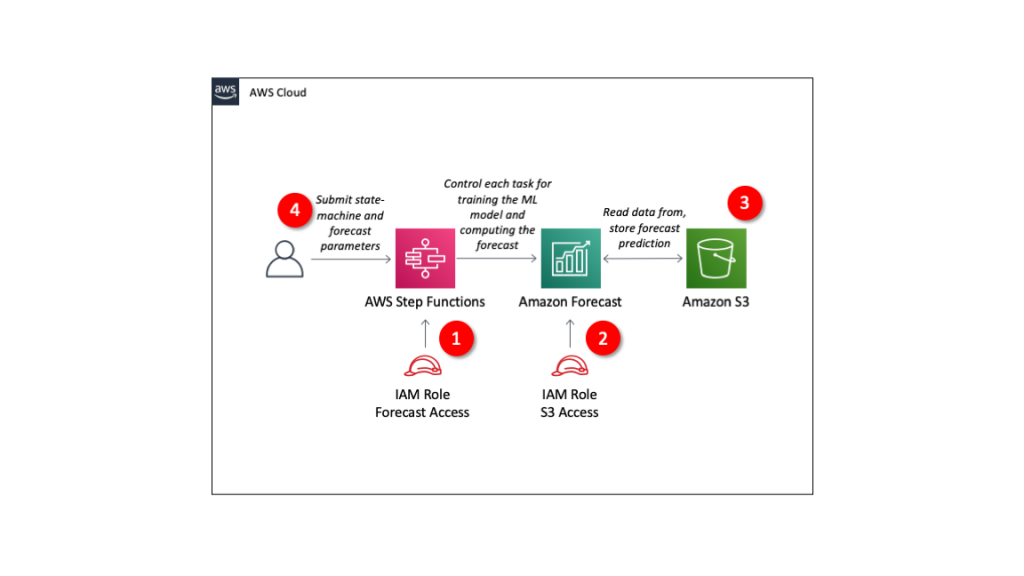
The solution includes four components:

Solution architecture

  1. IAM role granting Step Functions control over Forecast.
  2. IAM role granting Forecast access to S3 storage locations.
  3. S3 bucket with input data
  4. Define Step Functions state machine and parameters for Forecast.

The repo provides an AWS SAM template to deploy these resources in your AWS account.

Understanding Amazon Forecast

Amazon Forecast is a fully managed service for time series forecasting. Forecast uses machine learning to combine time series data with additional variables to build forecasts.

Using Amazon Forecast involves steps that may take from minutes to hours. Instead of executing each step and waiting for its completion, you use Step Functions to define the steps of the forecasting process.

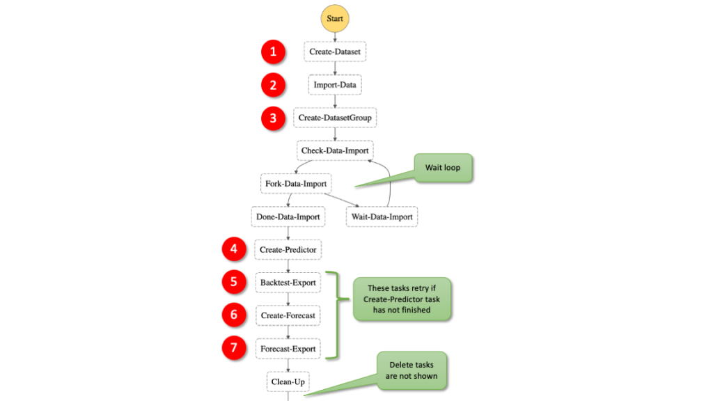
These are the individual steps of the Step Functions workflow:

Step Functions workflow

  1. Create a dataset: In Forecast, there are three types of datasets, target time series, related time series, and item metadata. The target time series is required and the others provide additional context with certain algorithms.
  2. Import data: This moves the information from S3 into a storage volume where the data is used for training and validation.
  3. Create a dataset group: This is the large box that isolates models and the data they are trained on from each other.
  4. Train a model: Forecast automates this process for you but you can also select algorithms. You can provide your own hyper parameters or use hyperparameter optimization (HPO) to determine the most performant values.
  5. Export back-test results: this creates a detailed table of the model performance.
  6. Deploy a predictor to deploy the model to use it to generate a forecast.
  7. Export forecast to create future predictions.

For more details, read the documentation of the Forecast APIs.

Example dataset

This example uses the individual household electric power consumption dataset. This dataset is available from the UCI Machine Learning Repository. We have aggregated the usage data to hourly intervals.

The dataset has three columns: the timestamp, value, and item ID. These are the minimum required to generate a forecast with Amazon Forecast.

Read more about the data and parameters in https://github.com/aws-samples/amazon-forecast-samples/tree/master/notebooks/basic/Tutorial.

Step Functions AWS SDK integrations

The AWS SDK integrations of Step Functions reduce the need for Lambda functions that call the Forecast APIs. You can call any AWS SDK-compatible service directly from the ASL. Use the following syntax in the resource field of a Step Functions task:

arn:aws:states:::aws-sdk:serviceName:apiAction.[serviceIntegrationPattern]

The following example compares using Step Functions AWS SDK service integrations with calling the boto3 Python method to create a dataset with a corresponding resource in the state machine definition. This is the ASL of a Step Functions state machine:

"States": {
  "Create-Dataset": {
    "Resource": "arn:aws:states:::aws-sdk:forecast:createDataset",
    "Parameters": {
      "DatasetName": "blog_example",
      "DataFrequency": "H",
      "Domain": "CUSTOM",
      "DatasetType": "TARGET_TIME_SERIES",
      "Schema": {
        "Attributes": [
          {
            "AttributeName": "timestamp",
            "AttributeType": "timestamp"
          },
          {
            "AttributeName": "target_value",
            "AttributeType": "float"
          },
          {
            "AttributeName": "item_id",
            "AttributeType": "string"
          }
        ]
      }
    },
    "ResultPath": "$.createDatasetResult",
    "Next": "Import-Data"
  }

The structure is similar to the corresponding boto3 methods. Compare the Python code with the state machine code – it uses the same parameters as calling the Python API:

forecast = boto3.client('forecast')
response = forecast.create_dataset(
             Domain='CUSTOM',
             DatasetType='TARGET_TIME_SERIES',
             DatasetName='blog_example',
             DataFrequency='H', 
             Schema={
               'Attributes': [
                  {
                    'AttributeName': 'timestamp',
                    'AttributeType': 'timestamp'
                  },
                  {
                    'AttributeName': 'target_value',
                    'AttributeType': 'float'
                  },
                  {
                    'AttributeName': 'item_id',
                    'AttributeType': 'string'
                  }
               ]
             }
           )

Handling asynchronous API calls

Several Forecast APIs run asynchronously, such as createDatasetImportJob and createPredictor. This means that your workflow must wait until the import job is completed.

You can use one of two methods in the state machine: create a wait loop, or allow any following task that depends on the completion of the previous task to retry.

In general, it is good practice to allow any task to retry for a few times. For simplicity this example does not include general error handling. Read the blog Handling Errors, Retries, and adding Alerting to Step Function State Machine Executions to learn more about writing robust state machines.

1. State machine wait loop

Wait loop

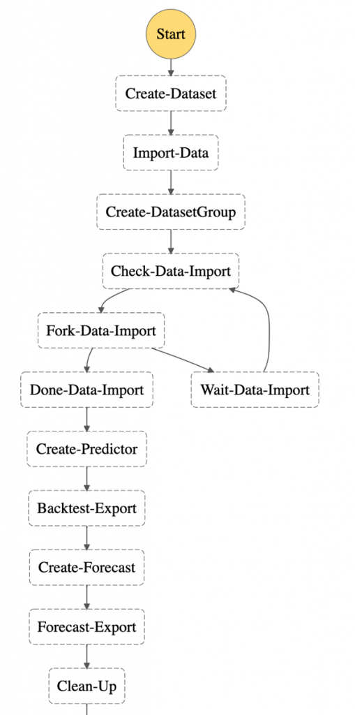
To wait for an asynchronous task to complete, use the services’ Describe* API methods to get the status of current job. You can implement the wait loop with the native Step Function tasks Choice and Wait.

Here, the task “Check-Data-Import” calls the describeDatasetImportJob API to receive a status value of the running job:

"Check-Data-Import": {
  "Type": "Task",
  "Resource": "arn:aws:states:::aws-sdk:forecast:describeDatasetImportJob",
  "Parameters": {
    "DatasetImportJobArn.$": "$.createDatasetImportJobResult.DatasetImportJobArn"
   },
   "ResultPath": "$.describeDatasetImportJobResult",
   "Next": "Fork-Data-Import"
 },
 "Fork-Data-Import": {
   "Type": "Choice",
   "Choices": [
     {
       "Variable": "$.describeDatasetImportJobResult.Status",
       "StringEquals": "ACTIVE",
       "Next": "Done-Data-Import"
     }
   ],
   "Default": "Wait-Data-Import"
 },
 "Wait-Data-Import": {
   "Type": "Wait",
   "Seconds": 60,
   "Next": "Check-Data-Import"
 },
 "Done-Data-Import": {
   "Type": "Pass",
   "Next": "Create-Predictor"
 },

2. Fail and retry

Alternatively, use the Retry parameter to specify how to repeat the API call in case of an error. This example shows how the attempt to create the forecast is repeated if the resource that it depends on is not created. In this case, the preceding task of creating the predictor.

The time between retries is set to 180 seconds and the number of retries must not exceed 100. This means that the workflow waits 3 minutes before trying again. The longest time to wait for the ML training is five hours.

With the BackoffRate set to 1, the wait interval of 3 minutes remains constant. Value greater that 1 may reduce the number of retries but may also add increased wait time for training jobs that run for several hours:

"Create-Forecast": {
  "Type": "Task",
  "Resource": "arn:aws:states:::aws-sdk:forecast:createForecast",
  "Parameters": {
    "ForecastName.$": "States.Format('{}_forecast', $.ProjectName)",
    "PredictorArn.$": "$.createPredictorResult.PredictorArn"
   },
   "ResultPath": "$.createForecastResult",
   "Retry": [
     {
       "ErrorEquals": ["Forecast.ResourceInUseException"],
       "IntervalSeconds": 180,
       "BackoffRate": 1.0,
       "MaxAttempts": 100
     }
   ],
   "Next": "Forecast-Export"
 },

Deploying the workflow

The AWS Serverless Application Model Command Line Interface (AWS SAM CLI) is an extension of the AWS CLI that adds functionality for building and testing serverless applications. Follow the instructions to install the AWS SAM CLI.

To build and deploy the application:

  1. Clone the GitHub repo:
    git clone https://github.com/aws-samples/aws-stepfunctions-examples/tree/main/sam/demo-forecast-service-integration
  2. Change directory to cloned repo.
    cd demo-forecast-service-integration
  3. Enable execute permissions for the deployment script
    chmod 700 ./bootstrap_deployment_script.sh
  4. Execute the script with a stack name of your choosing as parameter.
    ./bootstrap_deployment_script.sh <Here goes your stack name>

The script builds the AWS SAM template and deploys the stack under the given name. The AWS SAM template creates the underlying resources like S3 bucket, IAM policies, and Step Functions workflow. The script also copies the data file used for training to the newly created S3 bucket.

Running the workflow

After the AWS SAM Forecast workflow application is deployed, run the workflow to train a forecast predictor for the energy consumption:

  1. Navigate to the AWS Step Functions console.
  2. Select the state machine named “ForecastWorkflowStateMachine-*” and choose New execution.
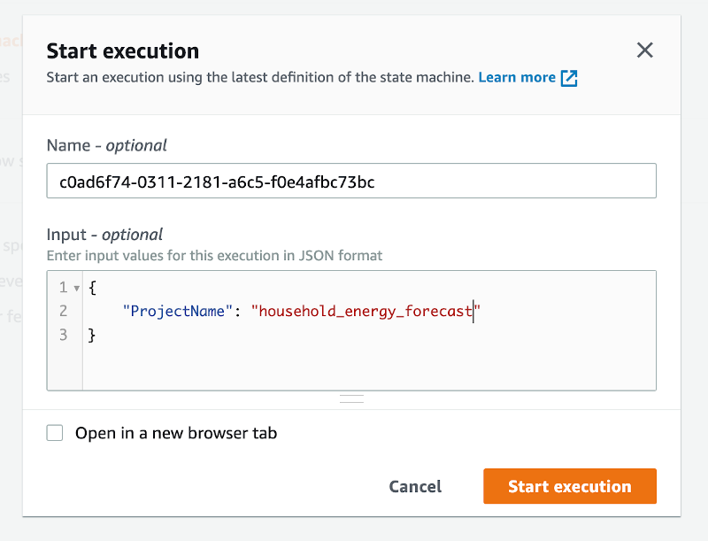
  3. Define the “ProjectName” parameter in form of a JSON structure. The name for the Forecast Dataset group is “household_energy_forecast”.
    Start execution
  4. Choose Start execution.

Viewing resources in the Amazon Forecast console

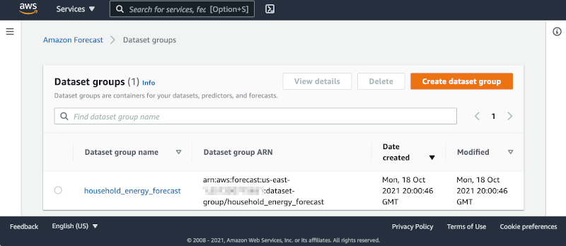
Navigate to the Amazon Forecast console and select the data set group “household_energy_forecast”. You can see the details of the Forecast resource as they are created. The provided state machine executes every step in the workflow and then deletes all resources, leaving the output files in S3.

Amazon Forecast console

You can disable the clean-up process by editing the state machine:

  1. Choose Edit to open the editor.
  2. Find the tasks “Clean-Up” and change the “Next” state from “Delete-Forecast_export” to “SuccessState”.
    "Clean-Up": {
       "Type": "Pass",
       "Next": "SuccessState"
    },
    
  3. Delete all tasks named Delete-*.

Remember to delete the dataset group manually if you bypass the clean-up process of the workflow.

Analyzing Forecast Results

The forecast workflow creates a folder “forecast_results” for all of its output files. In there you find the subfolders “backtestexport” with data produced by Backtest-Export task, and “forecast” with the predicted energy demand forecast produced by the Forecast-Export job.

The “backtestexport” folder contains two tables: “accuracy-metrics-values” with the model performance accuracy metrics, and “forecast-values” with the predicted forecast values of the training set. Read the blog post Amazon Forecast now supports accuracy measurements for individual items for details.

The forecast predictions are stored in the “forecast” folder. The table contains forecasts at three different quantiles: 10%, 50% and 90%.

The data files are partitioned into multiple CSV files. In order to analyze them, first download and merge the files into proper tables. Use the AWS CLI command to download

BUCKET="<your account number>-<your region>-sf-forecast-workflow"
aws s3 cp s3://$BUCKET/forecast_results . –recursive

Alternatively, you may import and analyze the data into Amazon Athena.

Cleaning up

To delete the application that you created, use the AWS SAM CLI.

sam delete --stack-name <Here goes your stack name>

Also delete the data files in the S3 bucket. If you skipped the clean-up tasks in your workflow, you must delete the dataset group from the Forecast console.

Important things to know

Here are things know, that will help you to use AWS SDK service integration:

  • Call AWS SDK services directly from the ASL in the resource field of a task state. To do this, use the following syntax: arn:aws:states:::aws-sdk:serviceName:apiAction.[serviceIntegrationPattern]
  • Use camelCase for apiAction names in the Resource field, such as “copyObject”, and use PascalCase for parameter names in the Parameters field, such as “CopySource”.
  • Step Functions cannot generate IAM policies for most AWS SDK service integrations. You must add those to the IAM role of the state machine explicitly.

Learn more about this new capability by reading its documentation.

Conclusion

This post shows how to create a Step Functions workflow for Forecast using AWS SDK service integrations, which allows you to use over 200 with AWS API actions. It shows two patterns for handling asynchronous tasks. The first pattern queries the describe-* API repeatedly and the second pattern uses the “Retry” option. This simplifies the development of workflows because in many cases they can replace Lambda functions.

For more serveless learning resources, visit Serverless Land.

Improving Retail Forecast Accuracy with Machine Learning

Post Syndicated from Soonam Jose original https://aws.amazon.com/blogs/architecture/improving-retail-forecast-accuracy-with-machine-learning/

The global retail market continues to grow larger and the influx of consumer data increases daily. The rise in volume, variety, and velocity of data poses challenges with demand forecasting and inventory planning. Outdated systems generate inaccurate demand forecasts. This results in multiple challenges for retailers. They are faced with over-stocking and lost sales, and often have to rely on increased levels of safety stock to avoid losing sales.

A recent McKinsey study indicates that AI-based forecasting improves forecasting accuracy by 10–20 percent. This translates to revenue increases of 2–3 percent. An accurate forecasting system can also help determine ideal inventory levels and better predict the impact of sales promotions. It provides a single view of demand across all channels and a better customer experience overall.

In this blog post, we will show you how to build a reliable retail forecasting system. We will use Amazon Forecast, and an AWS-vetted solution called Improving Forecast Accuracy with Machine Learning. This is an AWS Solutions Implementation that automatically produces forecasts and generates visualization dashboards. This solution can be extended to use cases across a variety of industries.

Improving Forecast Accuracy solution architecture

This post will illustrate a retail environment that has an SAP S/4 HANA system for overall enterprise resource planning (ERP). We will show a forecasting solution based on Amazon Forecast to predict demand across product categories. The environment also has a unified platform for customer experience provided by SAP Customer Activity Repository (CAR). Replenishment processes are driven by SAP Forecasting and Replenishment (F&R), and SAP Fiori apps are used to manage forecasts.

The solution is divided into four parts: Data extraction and preparation, Forecasting and monitoring, Data visualization, and Forecast import and utilization in SAP.

Figure 1. Notional architecture for improving forecasting accuracy solution and SAP integration

Figure 1. Notional architecture for improving forecasting accuracy solution and SAP integration

­­Data extraction and preparation

Historical demand data such as sales, web traffic, inventory numbers, and resource demand are extracted from SAP and uploaded to Amazon Simple Storage Service (S3). There are multiple ways to extract data from an SAP system into AWS. As part of this architecture, we will use operational data provisioning (ODP) extraction. ODP acts as a data source for OData services, enabling REST-based integrations with external applications. The ODP-Based Data Extraction via OData document details this approach. The steps involved are:

  1. Create a data source using transaction RSO2, allow Change Data Capture for specific data to be extracted
  2. Create an OData service using transaction SEGW
  3. Create a Data model for ODP extraction, which refers to the defined data source, then register the service
  4. Initiate the service from SAP gateway client
  5. In the AWS Management Console, create an AWS Lambda function to extract data and upload to S3. Check out the sample extractor code using Python, referenced in the blog Building data lakes with SAP on AWS

Related data that can potentially affect demand levels can be uploaded to Amazon S3. These could include seasonal events, promotions, and item price. Additional item metadata, such as product descriptions, color, brand, size may also be uploaded. Amazon Forecast provides built-in related time series data for holidays and weather. These three components together form the forecast inputs.

Forecasting and monitoring

An S3 event notification will be initiated when new datasets are uploaded to the input bucket. This in turn, starts an AWS Step Functions state machine. The state machine combines a series of AWS Lambda functions that build, train, and deploy machine learning models in Amazon Forecast. All AWS Step Functions logs are sent to Amazon CloudWatch. Administrators will be notified with the results of the AWS Step Functions through Amazon Simple Notification Service (SNS).

An AWS Glue job combines raw forecast input data, metadata, predictor backtest exports, and forecast exports. These all go into an aggregated view of forecasts in an S3 bucket. It is then translated to the format expected by the External Forecast import interface. Amazon Athena can be used to query forecast output in S3 using standard SQL queries.

Data visualization

Amazon QuickSight analyses can be created on a per-forecast basis. This provides users with forecast output visualization across hierarchies and categories of forecasted items. It also displays item-level accuracy metrics. Dashboards can be created from these analyses and shared within the organization. Additionally, data scientists and developers can prepare and process data, and evaluate Forecast outputs using an Amazon SageMaker Notebook Instance.

Forecast import and utilization in SAP

Amazon Forecast outputs located in Amazon S3 will be imported into the Unified Demand Forecast (UDF) module within the SAP Customer Activity Repository (CAR). You can read here about how to import external forecasts. An AWS Lambda function will be initiated when aggregated forecasts are uploaded to the S3 bucket. The Lambda function performs a remote function call (RFC) to the SAP system through the official SAP JCo Library. The SAP RFC credentials and connection information may be stored securely inside AWS Secrets Manager and read on demand to establish connectivity.

Once imported, forecast values from the solution can be retrieved by SAP Forecasting and Replenishment (F&R). They will be consumed as an input to replenishment processes, which consist of requirements calculation and­­­­­ requirement quantity optimization. SAP F&R calculates requirements based on the forecast, the current stock, and the open purchase orders. The requirement quantity then may be improved in accordance with optimization settings defined in SAP F&R.

­­­

Additionally, you have the flexibly to adjust the system forecast as required by the demand situation or analyze forecasts via respective SAP Fiori Apps.

Sample use case: AnyCompany Stores, Inc.

To illustrate how beneficial this solution can be for retail organizations, let’s consider AnyCompany Stores, Inc. This is a hypothetical customer and leader in the retailer industry with 985 stores across the United States. They struggle with issues stemming from their existing forecasting implementation. That implementation only understands certain categories and does not factor in the entire product portfolio. Additionally, it is limited to available demand history and does not consider related information that may affect forecasts. AnyCompany Stores is looking to improve their demand forecasting system.

Using Improving Forecast Accuracy with Machine Learning, AnyCompany Stores can easily generate AI-based forecasts at appropriate quantiles to address sensitivities associated with respective product categories. This mitigates inconsistent inventory buys, overstocks, out-of-stocks, and margin erosion. The solution also considers all relevant related data in addition to the historical demand data. This ensures that generated forecasts are accurate for each product category.

The generated forecasts may be used to complement existing forecasting and replenishment processes. With an improved forecasting solution, AnyCompany Stores will be able to meet demand, while holding less inventory and improving customer experience. This also helps ensure that potential demand spikes are accurately captured, so staples will always be in stock. Additionally, the company will not overstock expensive items with short shelf lives that are likely to spoil.

Conclusion

In this post, we explored how to implement an accurate retail forecasting solution using a ready-to-deploy AWS Solution. We use generated forecasts to drive inventory replenishment optimization and improve customer experience. The solution can be extended to inventory, workforce, capacity, and financial planning.

We showcase one of the ways in which Improving Forecast Accuracy with Machine Learning may be extended for a use case in the retail industry. If your organization would like to improve business outcomes with the power of forecasting, explore customizing this solution to fit your unique needs.

Further reading: