Post Syndicated from Kevin Guthrie original https://blog.cloudflare.com/loving-performance-measurements/
⚠️ WARNING ⚠️ This blog post contains graphic depictions of probability. Reader discretion is advised.
Measuring performance is tricky. You have to think about accuracy and precision. Are your sampling rates high enough? Could they be too high?? How much metadata does each recording need??? Even after all that, all you have is raw data. Eventually for all this raw performance information to be useful, it has to be aggregated and communicated. Whether it’s in the form of a dashboard, customer report, or a paged alert, performance measurements are only useful if someone can see and understand them.
This post is a collection of things I’ve learned working on customer performance escalations within Cloudflare and analyzing existing tools (both internal and commercial) that we use when evaluating our own performance. A lot of this information also comes from Gil Tene’s talk, How NOT to Measure Latency. You should definitely watch that too (but maybe after reading this, so you don’t spoil the ending). I was surprised by my own blind spots and which assumptions turned out to be wrong, even though they seemed “obviously true” at the start. I expect I am not alone in these regards. For that reason this journey starts by establishing fundamental definitions and ends with some new tools and techniques that we will be sharing as well as the surprising results that those tools uncovered.
So … what is performance? Alright, let’s start with something easy: definitions. “Performance” is not a very precise term because it gets used in too many contexts. Most of us as nerds and engineers have a gut understanding of what it means, without a real definition. We can’t really measure it because how “good” something is depends on what makes that thing good. “Latency” is better … but not as much as you might think. Latency does at least have an implicit time unit, so we can measure it. But … what is latency? There are lots of good, specific examples of measurements of latency, but we are going to use a general definition. Someone starts something, and then it finishes — the elapsed time between is the latency.

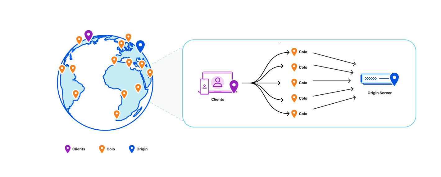
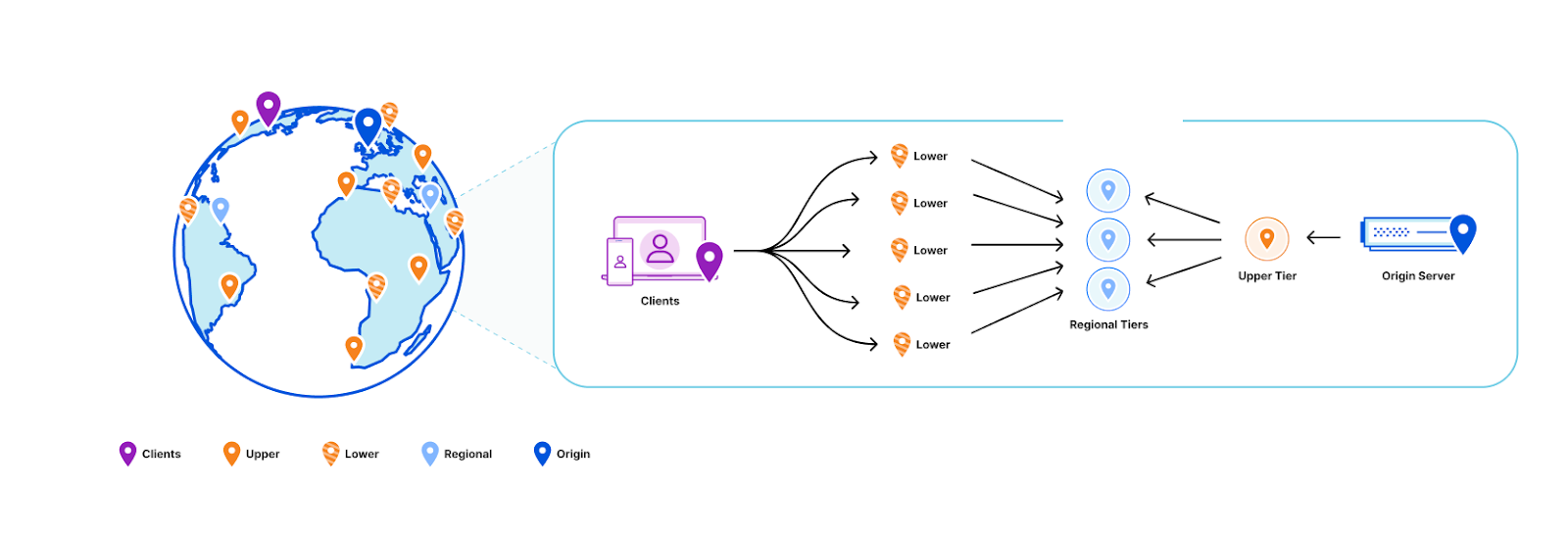
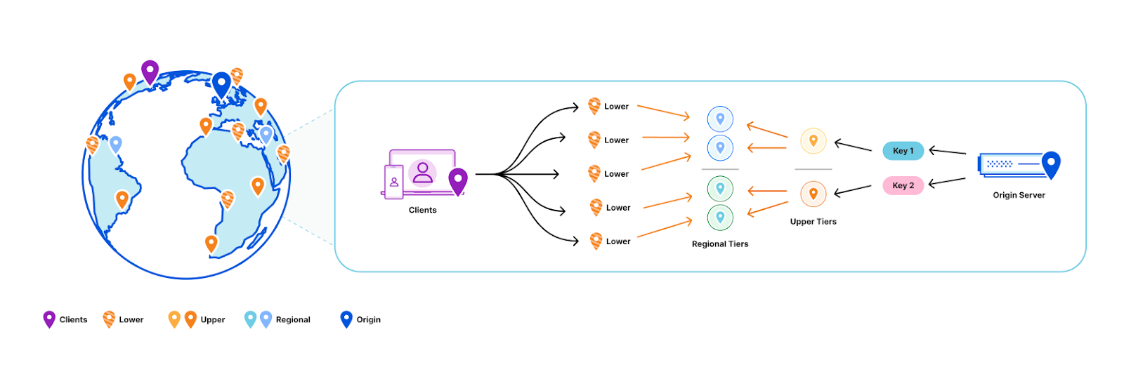
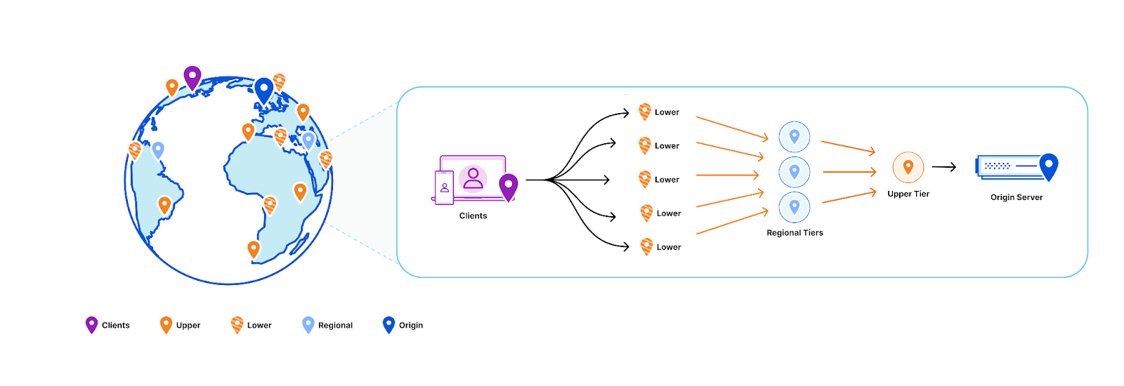
This seems a bit reductive, but it’s a surprisingly useful definition because it gives us a key insight. This fundamental definition of latency is based around the client’s perspective. Indeed, when we look at our internal measurements of latency for health checks and monitoring, they all have this one-sided caller/callee relationship. There is the latency of the caching layer from the point of view of the ingress proxy. There’s the latency of the origin from the cache’s point of view. Each component can measure the latency of its upstream counterparts, but not the other way around.
This one-sided nature of latency observation is a real problem for us because Cloudflare only exists on the server side. This makes all of our internal measurements of latency purely estimations. Even if we did have full visibility into a client’s request timing, the start-to-finish latency of a request to Cloudflare isn’t a great measure of Cloudflare’s latency. The process of making an HTTP request has lots of steps, only a subset of which are affected by us. Time spent on things like DNS lookup, local computation for TLS, or resource contention do affect the client’s experience of latency, but only serve as sources of noise when we are considering our own performance.
There is a very useful and common metric that is used to measure web requests, and I’m sure lots of you have been screaming it in your brains from the second you read the title of this post. ✨Time to first byte✨. Clearly this is the answer, right?! But … what is “Time to first byte”?
Time to first byte (TTFB) on its face is simple. The name implies that it’s the time it takes (on the client’s side) to receive the first byte of the response from the server, but unfortunately, that only describes when the timer should end. It doesn’t say when the timer should start. This ambiguity is just one factor that leads to inconsistencies when trying to compare TTFB across different measurement platforms … or even across a single platform because there is no one definition of TTFB. Similar to “performance”, it is used in too many places to have a single definition. That being said, TTFB is a very useful concept, so in order to measure it and report it in an unambiguous way, we need to pick a definition that’s already in use.
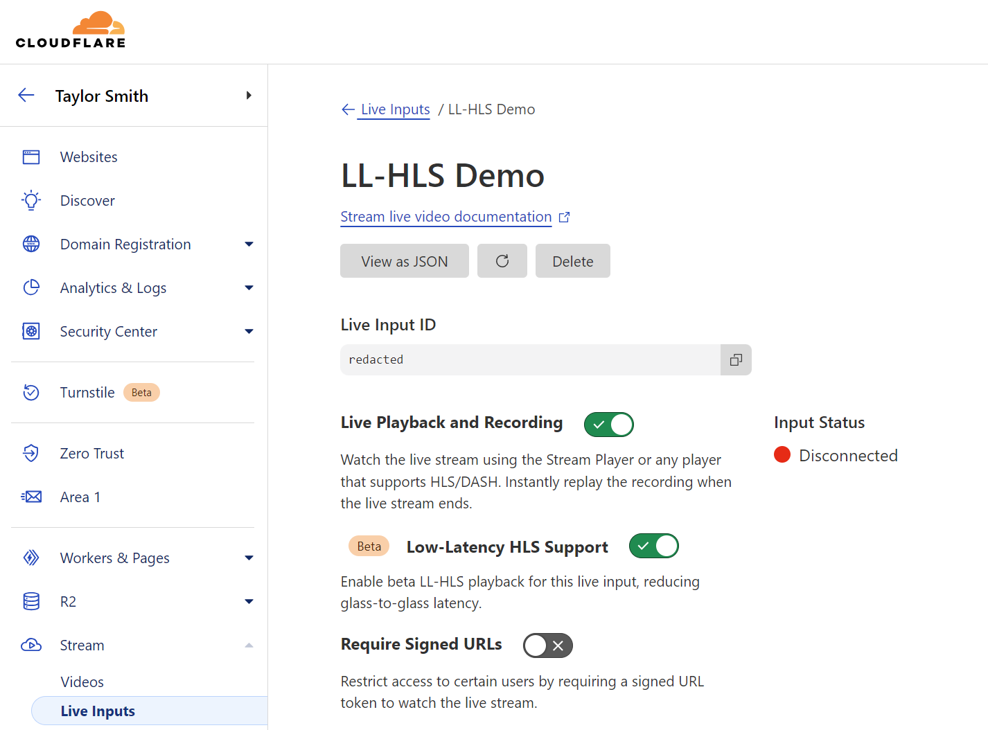
We have mentioned TTFB in other blog posts, but this one sums up the problem best with “Time to first byte isn’t what it used to be.” You should read that article too, but the gist is that one popular TTFB definition used by browsers was changed in a confusing way with the introduction of early hints in June 2022. That post and others make the point that while TTFB is useful, it isn’t the best direct measurement for web performance. Later on in this post we will derive why that’s the case.
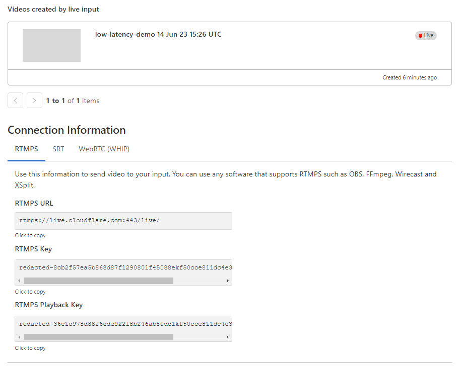
One common place we see TTFB used is our customers’ analysis comparing Cloudflare’s performance to our competitors through Catchpoint. Customers, as you might imagine, have a vested interest in measuring our latency, as it affects theirs. Catchpoint provides several tools built on their global Internet probe network for measuring HTTP request latency (among other things) and visualizing it in their web interface. In an effort to align better with our customers, we decided to adopt Catchpoint’s terminology for talking about latency, both internally and externally.
While Catchpoint makes things like TTFB easy to plot over time, the visualization tool doesn’t give a definition of what TTFB is, but after going through all of their technical blog posts and combing through thousands of lines of raw data, we were able to get functional definitions for TTFB and other composite metrics. This was an important step because these metrics are how our customers are viewing our performance, so we all need to be able to understand exactly what they signify! The final report for this is internal (and long and dry), so in this post, I’ll give you the highlights in the form of colorful diagrams, starting with this one.

This diagram shows our customers’ most commonly viewed client metrics on Catchpoint and how they fit together into the processing of a request from the server side. Notice that some are directly measured, and some are calculated based on the direct measurements. Right in the middle is TTFB, which Catchpoint calculates as the sum of the DNS, Connect, TLS, and Wait times. It’s worth noting again that this is not the definition of TTFB, this is just Catchpoint’s definition, and now ours.
This breakdown of HTTPS phases is not the only one commonly used. Browsers themselves have a standard for measuring the stages of a request. The diagram below shows how most browsers are reporting request metrics. Luckily (and maybe unsurprisingly) these phases match Catchpoint’s very closely.

There are some differences beyond the inclusion of things like AppCache and Redirects (which are not directly impacted by Cloudflare’s latency). Browser timing metrics are based on timestamps instead of durations. The diagram subtly calls this out with gaps between the different phases indicating that there is the potential for the computer running the browser to do things that are not part of any phase. We can line up these timestamps with Catchpoint’s metrics like so:

Now that we, our customers, and our browsers (with data coming from RUM) have a common and well-defined language to talk about the phases of a request, we can start to measure, visualize, and compare the components that make up the network latency of a request.
Now that we have defined what our key values for latency are, we can record numbers and put them in a chart and watch them roll by … except not directly. In most cases, the systems we use to record the data actively prevent us from seeing the recorded data in its raw form. Tools like Prometheus are designed to collect pre-aggregated data, not individual samples, and for a good reason. Storing every recorded metric (even compacted) would be an enormous amount of data. Even worse, the data loses its value exponentially over time, since the most recent data is the most actionable.
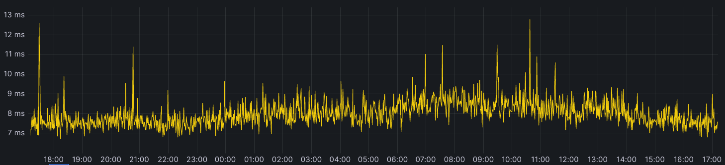
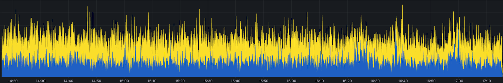
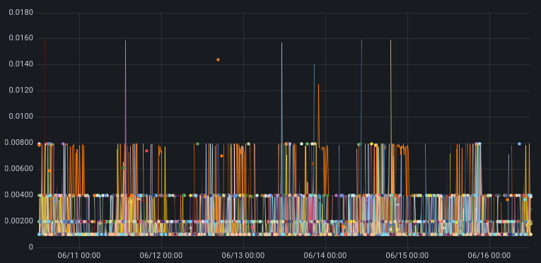
The unavoidable conclusion is that some aggregation has to be done before performance data can be visualized. In most cases, the aggregation means looking at a series of windowed percentiles over time. The most common are 50th percentile (median), 75th, 90th, and 99th if you’re really lucky. Here is an example of a latency visualization from one of our own internal dashboards.

It clearly shows a spike in latency around 14:40 UTC. Was it an incident? The p99 jumped by 1300% (500ms to 6500
ms) for multiple minutes while the p50 jumped by more than 13600% (4.4ms to 600ms). It is a clear signal, so something must have happened, but what was it? Let me keep you in suspense for a second while we talk about statistics and probability.
Let me start with a quote from my dear, close, personal friend @ThePrimeagen:

It’s a good reminder that while statistics is a great tool for providing a simplified and generalized representation of a complex system, it can also obscure important subtleties of that system. A good way to think of statistical modeling is like lossy compression. In the latency visualization above (which is a plot of TTFB over time), we are compressing the entire spectrum of latency metrics into 4 percentile bands, and because we are only considering up to the 99th percentile, there’s an entire 1% of samples left over that we are ignoring!
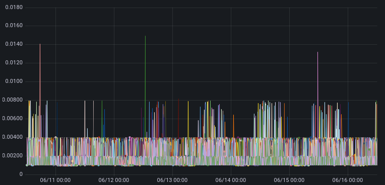
“What?” I hear you asking. “P99 is already well into perfection territory. We’re not trying to be perfectionists. Maybe we should get our p50s down first”. Let’s put things in perspective. This zone (www.cloudflare.com) is getting about 30,000 req/s and the 99th percentile latency is 500 ms. (Here we are defining latency as “Edge TTFB”, a server-side approximation of our now official definition.) So there are 300 req/s that are taking longer than half a second to complete, and that’s just the portion of the request that we can see. How much worse than 500 ms are those requests in the top 1%? If we look at the 100th percentile (the max), we get a much different vibe from our Edge TTFB plot.

Viewed like this, the spike in latency no longer looks so remarkable. Without seeing more of the picture, we could easily believe something was wrong when in reality, even if something is wrong, it is not localized to that moment. In this case, it’s like we are using our own statistics to lie to ourselves.
Maybe you’re still not convinced. It feels more intuitive to focus on the median because the latency experienced by 50 out of 100 people seems more important to focus on than that of 1 in 100. I would argue that is a totally true statement, but notice I said “people” and not “requests.” A person visiting a website is not likely to be doing it one request at a time.
Taking www.cloudflare.com as an example again, when a user opens that page, their browser makes more than 70 requests. It sounds big, but in the world of user-facing websites, it’s not that bad. In contrast, www.amazon.com issues more than 400 requests! It’s worth noting that not all those requests need to complete before a web page or application becomes usable. That’s why more advanced and browser-focused metrics exist, but I will leave a discussion of those for later blog posts. I am more interested in how making that many requests changes the probability calculations for expected latency on a per-user basis.
Here’s a brief primer on combining probabilities that covers everything you need to know to understand this section.
-
The probability of two things happening is the probability of the first happening multiplied by the probability of the second thing happening. $$P(X\cap Y )=P(X) \times P (Y)$$
-
The probability of something in the $X^{th}$ percentile happening is $X\%$. $$P(pX) = X\%$$
Let’s define $P( pX_{N} )$ as the probability that someone on a website with $N$ requests experiences no latencies >= the $X^{th}$ percentile. For example, $P(p50_{2})$ would be the probability of getting no latencies greater than the median on a page with 2 requests. This is equivalent to the probability of one request having a latency less than the $p50$ and the other request having a latency less than the $p50$. We can use the first identities above.
$$\begin{align}
P( p50_{2}) &= P\left ( p50 \cap p50 \right ) \\
&= P( p50) \times P\left ( p50 \right ) \\
&= 50\%^{2} \\
&= 25\%
\end{align}$$
We can generalize this for any percentile and any number of requests. $$P( pX_{N}) = X\%^{N}$$
For www.cloudflare.com and its 70ish requests, the percentage of visitors that won’t experience a latency above the median is
$$\begin{align}
P( p50_{70}) &= 50\%^{70} \\
&\approx 0.000000000000000000001\%
\end{align}$$
This vanishingly small number should make you question why we would value the $p50$ latency so highly at all when effectively no one experiences it as their worst case latency.
So now the question is, what request latency percentile should we be looking at? Let’s go back to the statement at the beginning of this section. What does the median person experience on www.cloudflare.com? We can use a little algebra to solve for that.
$$\begin{align}
P( pX_{70}) &= 50\% \\
X^{70} &= 50\% \\
X &= e^{ \frac{ln\left ( 50\% \right )}{70}} \\
X &\approx 99\%
\end{align}$$
This seems a little too perfect, but I am not making this up. For www.cloudflare.com, if you want to capture a value that’s representative of what the median user can expect, you need to look at $p99$ request latency. Extending this even further, if you want a value that’s representative of what 99% of users will experience, you need to look at the 99.99th percentile!
Okay, this is where we bring everything together, so stay with me. So far, we have only talked about measuring the performance of a single system. This gives us absolute numbers to look at internally for monitoring, but if you’ll recall, the goal of this post was to be able to clearly communicate about performance outside the company. Often this communication takes the form of comparing Cloudflare’s performance against other providers. How are these comparisons done? By plotting a percentile request “latency” over time and eyeballing the difference.

With everything we have discussed in this post, it seems like we can devise a better method for doing this comparison. We saw how exposing more of the percentile spectrum can provide a new perspective on existing data, and how impactful higher percentile statistics can be when looking at a more complete user experience. Let me close this post with an example of how putting those two concepts together yields some intriguing results.
Below is a comparison of the latency (defined here as the sum of the TLS, Connect, and Wait times or the equivalent of TTFB – DNS lookup time) for the customer when viewed through Cloudflare and a competing provider. This is the same data represented in the chart immediately above (containing 90,000 samples for each provider), just in a different form called a CDF plot, which is one of a few ways we are making it easier to visualize the entire percentile range. The chart shows the percentiles on the y-axis and latency measurements on the x-axis, so to see the latency value for a given percentile, you go up to the percentile you want and then over to the curve. Interpreting these charts is as easy as finding which curve is farther to the left for any given percentile. That curve will have the lower latency.

It’s pretty clear that for nearly the entire percentile range, the other provider has the lower latency by as much as 30ms. That is, until you get to the very top of the chart. There’s a little bit of blue that’s above (and therefore to the left) of the green. In order to see what’s going on there more clearly, we can use a different kind of visualization. This one is called a QQ-Plot, or quantile-quantile plot. This shows the same information as the CDF plot, but now each point on the represents a specific quantile, and the 2 axes are the latency values of the two providers at that percentile.

This chart looks complicated, but interpreting it is similar to the CDF plot. The blue is a dividing marker that shows where the latency of both providers is equal. Points below the line indicate percentiles where the other provider has a lower latency than Cloudflare, and points above the line indicate percentiles where Cloudflare is faster. We see again that for most of the percentile range, the other provider is faster, but for percentiles above 99, Cloudflare is significantly faster.
This is not so compelling by itself, but what if we take into account the number of requests this page issues … which is over 180. Using the same math from above, and only considering half the requests to be required for the page to be considered loaded, yields this new effective QQ plot.

Taking multiple requests into account, we see that the median latency is close to even for both Cloudflare and the other provider, but the stories above and below that point are very different. A user has about an even chance of an experience where Cloudflare is significantly faster and one where Cloudflare is slightly slower than the other provider. We can show the impact of this shift in perspective more directly by calculating the expected value for request and experienced latency.
|
Latency Kind |
Cloudflare (ms) |
Other CDN (ms) |
Difference (ms) |
|
Expected Request Latency |
141.9 |
129.9 |
+12.0 |
|
Expected Experienced Latency Based on 90 Requests |
207.9 |
281.8 |
-71.9 |
Shifting the focus from individual request latency to user latency we see that Cloudflare is 70 ms faster than the other provider. This is where our obsession with reliability and tail latency becomes a win for our customers, but without a large volume of raw data, knowledge, and tools, this win would be totally hidden. That is why in the near future we are going to be making this tool and others available to our customers so that we can all get a more accurate and clear picture of our users’ experiences with latency. Keep an eye out for more announcements to come later in 2025.