Apache Airflow orchestrates data pipelines ranging from data ingestion and machine learning to SQL-based analytics. Some analytical workloads, such as daily rollups and usage reports, process bounded datasets and can run within the resources of a single worker. For these workloads, deploying a distributed query cluster can add unnecessary infrastructure and operational complexity.
DuckDB is an open source in-process analytical database that runs within an application without requiring a separate database server. Its columnar, vectorized execution engine supports analytical SQL operations, including scans, joins, and aggregations.
Amazon Managed Workflows for Apache Airflow (Amazon MWAA) runs Apache Airflow as a managed service, so you can schedule, run, and monitor workflows without managing the underlying Airflow infrastructure. Combined with DuckDB, you can add SQL transformations to your pipelines that run inside the Airflow task itself.
In this post, you learn how to run DuckDB with an Amazon MWAA Provisioned environment.
How DuckDB and Amazon MWAA work together
In Apache Airflow, a directed acyclic graph (DAG) defines tasks and their dependencies, along with scheduling, retry, and concurrency settings. Amazon MWAA runs the tasks on workers and publishes configured task logs to Amazon CloudWatch Logs.
DuckDB runs in the Airflow task process, using the CPU, memory, and local storage of the Amazon MWAA worker container. Amazon MWAA orchestrates the workflow, while DuckDB performs the SQL processing.
This walkthrough uses DuckDB 2.0.0, which includes asynchronous I/O for reading from object storage and first-class VARIANT support for semi-structured data. DuckDB 2.0.0 also supports a client-server mode through the Quack protocol, which lets other processes connect to a DuckDB database over the network. This walkthrough runs DuckDB in-process because each Airflow task performs a self-contained transformation.
Introducing the Apache Airflow DuckDB provider
The Apache Airflow DuckDB provider provides the DuckDBExecuteQueryOperator. The operator runs DuckDB locally in the worker container and executes SQL without starting a separate query service.
The DuckDB integration in the Amazon provider adds the AWS aware duckdb_aws connection type. On supported Amazon MWAA Provisioned environments, the DuckDB packages are preinstalled, and Amazon MWAA creates the default connection, as described later in this post.
Solution overview
An engineering team operates a shared inference service that product teams use for their applications. As usage grows, the team needs to understand which applications and teams are driving inference activity and the estimated cost of that usage. Showback provides an itemized view of usage and estimated cost without charging teams directly.
To build the showback pipeline without a separate analytics cluster, the team uses Amazon MWAA to orchestrate Airflow tasks that run DuckDB. DuckDB reads source files from Amazon Simple Storage Service (Amazon S3), performs SQL transformations, and publishes the results as Apache Iceberg tables in Amazon S3 Tables. This pattern suits bounded, SQL-oriented workloads that run reliably within the resources of a single worker.
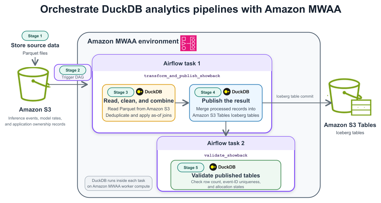
Figure 1: Amazon MWAA orchestrates two DuckDB tasks across five stages, from reading Parquet data in Amazon S3 through publishing and validating Iceberg tables in Amazon S3 Tables
The workflow has five logical stages, implemented by two Airflow tasks, as shown in Figure 1.
Stage 1: Store the source data – An Amazon S3 bucket stores the Parquet files for inference events, model rates, and application ownership records.
Stage 2: Trigger the DAG – A manual action starts this example DAG. Amazon MWAA orchestrates both tasks, tracks their status, and sends task logs to Amazon CloudWatch Logs. You can configure a schedule for recurring runs.
Stage 3: Read, clean, and combine the records – The transform_and_publish_showback task uses DuckDB to read the Parquet files directly from Amazon S3, deduplicate events, and apply the model rate and ownership record effective at each invocation timestamp.
Stage 4: Publish the result – In the same transform_and_publish_showback task, DuckDB merges the processed records into the costed_invocations Iceberg table in Amazon S3 Tables and commits the update. The task also creates the daily_application_showback and team_budget_status summary tables.
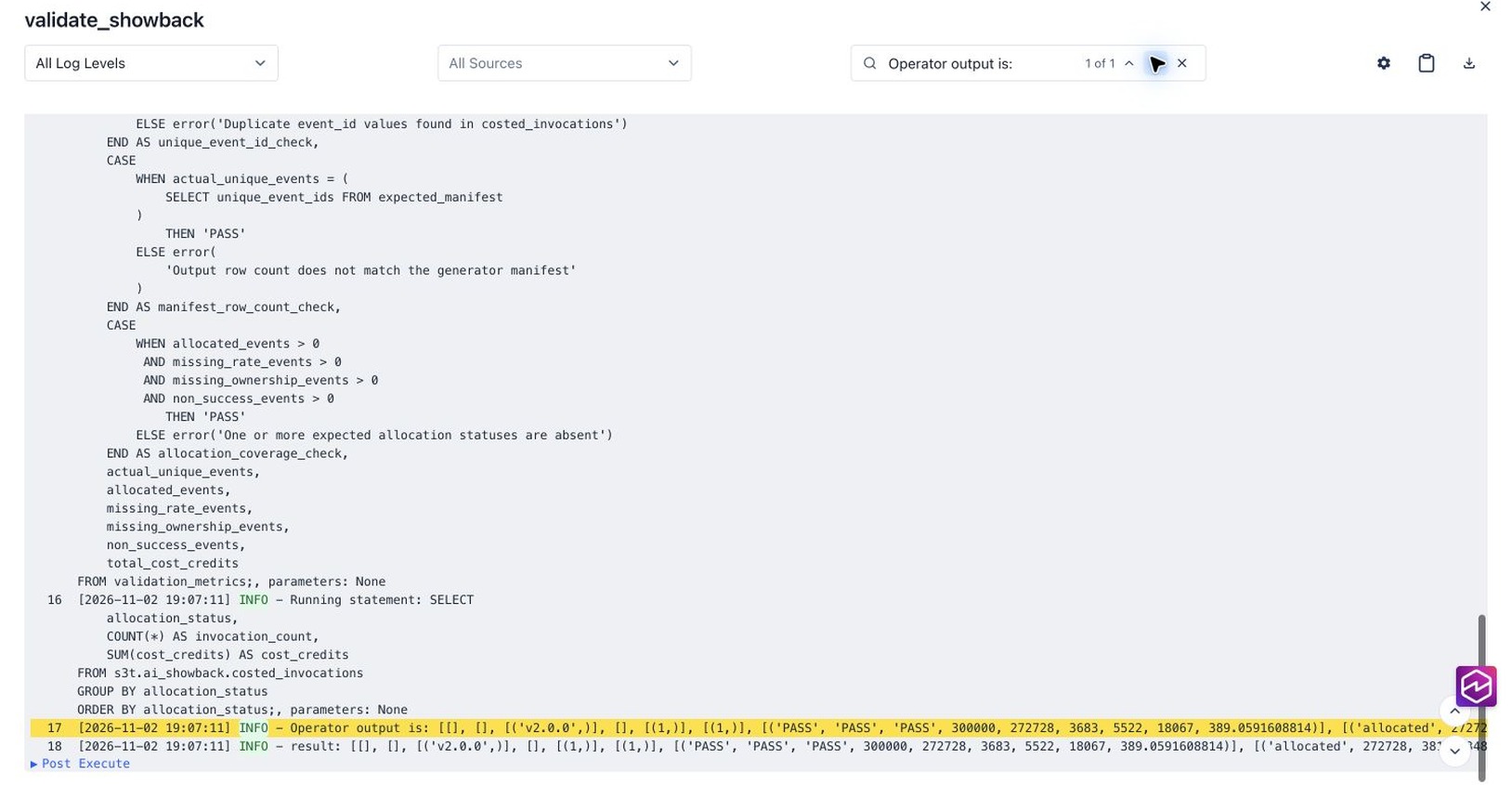
Stage 5: Validate published tables – After publication, the second Airflow task, validate_showback, uses DuckDB to check the row count, confirm that event IDs are unique, and verify the expected allocation states.
The sample rates and cost_credits values are synthetic and are provided only to demonstrate allocation logic. They do not represent AWS pricing, Amazon Bedrock charges, or customer billing records.
Prerequisites
Before you begin, make sure you have the following resources and permissions:
An Amazon MWAA Provisioned environment running Apache Airflow 3.3.1 with Python 3.12. See Apache Airflow versions on Amazon MWAA for the currently supported versions.
An Amazon S3 bucket for the source Parquet files and an Amazon S3 Tables table bucket for the outputs.
An Amazon MWAA execution role with read access to the source bucket and permissions to create, read, and update tables and table data in the target table bucket. For the required actions, see Accessing Amazon S3 Tables using open source applications. If the table bucket uses a customer managed AWS Key Management Service (AWS KMS) key, the role also needs permission to use that key.
Network connectivity from the Amazon MWAA private subnets to Amazon S3 and Amazon S3 Tables. This sample installs the DuckDB Iceberg extension at runtime, so it also requires access to the official DuckDB extension repository unless the matching extension is already available.
The sample bundle containing the DAG, SQL, and synthetic-data generator used in this walkthrough.
Python 3, the dependencies listed in generator-requirements.txt, and the AWS Command Line Interface (AWS CLI) configured on the workstation where you generate and upload the sample data.
In the test environment used for this post, Amazon MWAA included apache-airflow-providers-amazon 9.38.0, apache-airflow-providers-duckdb 0.2.0, and DuckDB 2.0.0. These versions might change in future Amazon MWAA releases.
Use the built-in DuckDB providers and connection
Amazon MWAA Provisioned environments running Apache Airflow 3.3.1 include DuckDB, the Apache Airflow DuckDB provider, and the DuckDB integration in the Amazon provider. Amazon MWAA also creates a connection named duckdb_default with the connection type duckdb_aws. You do not need to add packages to requirements.txt or create the connection manually.
To confirm that the connection exists, choose Admin, then Connections in the Airflow UI. Look for duckdb_default.
Note: When a DuckDBExecuteQueryOperator task doesn’t specify conn_id, it uses duckdb_default. The AWS aware hook obtains temporary credentials from the Amazon MWAA execution role and creates a DuckDB S3 secret for the task. Don’t put AWS access keys in the DAG or create a separate S3 secret in the SQL, because doing so can conflict with the secret the hook creates. If duckdb_default doesn’t appear under Admin, Connections, update your Amazon MWAA environment without changing any settings to apply the latest Amazon MWAA image.
Prepare the sample data
Use generate_ai_inference_data.py from the sample bundle to create Parquet files containing inference events, model rates, and application ownership records. A fixed random seed makes the input reproducible. The dataset includes duplicate events and changes to rates and ownership, allowing you to demonstrate deduplication and effective-dated attribution.
Run the generator and upload the resulting files to Amazon S3:
The default settings generate approximately 300,000 unique events across daily partitions. The generated manifest.json records the expected unique-event count for subsequent validation.
Build the DuckDB transformation
See publish_showback.sql in the sample bundle for the complete transformation SQL. The following excerpts highlight three operations used in the pipeline.
Read Parquet files and remove duplicates
The read_parquet function reads daily Parquet partitions directly from Amazon S3. The union_by_name option aligns columns across files with different schemas. A ROW_NUMBER window function retains the record with the most recent ingestion timestamp for each event ID.
CREATE OR REPLACE TEMP TABLE latest_events AS
SELECT *
FROM read_parquet(
    's3://<SOURCE-BUCKET>/ai-showback/'
    'inference_events/ingest_date=*/*.parquet',
    hive_partitioning = true,
    union_by_name = true
)
QUALIFY ROW_NUMBER() OVER (
    PARTITION BY event_id
    ORDER BY ingested_at DESC
) = 1;
Apply rates and ownership at the event time
Model rates and application ownership can change over time. Using only the current reference record would misattribute historical events. The DuckDB ASOF LEFT JOIN selects the latest reference record whose effective timestamp is no later than the event timestamp.
CREATE OR REPLACE TEMP TABLE events_with_rates AS
SELECT
    e.*,
    r.input_credits_per_million,
    r.output_credits_per_million
FROM latest_events AS e
ASOF LEFT JOIN read_parquet(
    's3://<SOURCE-BUCKET>/ai-showback/reference/model_rates.parquet'
) AS r
ON e.model_id = r.model_id
AND e.event_ts >= r.effective_from;

CREATE OR REPLACE TEMP TABLE costed_batch AS
SELECT
    e.*,
    o.team_id,
    o.cost_center,
    (
        e.input_tokens * e.input_credits_per_million
        + e.output_tokens * e.output_credits_per_million
    ) / 1000000.0 AS cost_credits
FROM events_with_rates AS e
ASOF LEFT JOIN read_parquet(
    's3://<SOURCE-BUCKET>/ai-showback/'
    'reference/application_ownership.parquet'
) AS o
ON e.application_id = o.application_id
AND e.event_ts >= o.effective_from;
The full sample retains events without matching reference records and assigns an allocation status. This makes missing rate or ownership data visible during validation rather than excluding those events.
Publish retry-safe Iceberg output
Set the DuckDB session timezone to UTC, attach the Amazon S3 Tables table bucket as an Iceberg catalog, then merge the transformed records using a stable event ID:
INSTALL iceberg;
LOAD iceberg;
SET TimeZone = 'UTC';

ATTACH 'arn:aws:s3tables:<REGION>:<ACCOUNT-ID>:bucket/<TABLE-BUCKET>'
AS s3t (TYPE iceberg, ENDPOINT_TYPE s3_tables);

CREATE SCHEMA IF NOT EXISTS s3t.ai_showback;

MERGE INTO s3t.ai_showback.costed_invocations AS target
USING costed_batch AS source
ON target.event_id = source.event_id
WHEN MATCHED THEN UPDATE SET
    ingested_at = source.ingested_at,
    team_id = source.team_id,
    cost_center = source.cost_center,
    cost_credits = source.cost_credits
WHEN NOT MATCHED THEN INSERT BY NAME;
For daily_application_showback, use every grouped dimension in the MERGE condition. Use null-safe comparisons for nullable dimensions so that a retry cannot match multiple grouped source rows to one target row:
ON target.usage_date = source.usage_date
AND target.application_id = source.application_id
AND target.team_id IS NOT DISTINCT FROM source.team_id
AND target.cost_center IS NOT DISTINCT FROM source.cost_center
AND target.model_id = source.model_id
AND target.use_case IS NOT DISTINCT FROM source.use_case
The sample uses an unpartitioned tutorial table because support for update and delete operations can vary by DuckDB and Iceberg version. Validate table creation, the write pattern, partition design, partial-failure behavior, and reruns with the versions you deploy. An Iceberg snapshot commit is atomic for one table, but commits to the three output tables are not a single transaction.
Create the Amazon MWAA DAG
The duckdb_ai_inference_showback.py file in the sample bundle contains the complete Apache Airflow 3.3.1 DAG. It uses the public airflow.sdk import and a timezone-aware start date. Because schedule=None, you trigger it manually. You can add a schedule for recurring runs. The publication task runs before validation. Setting max_active_runs=1 prevents overlapping runs of this DAG. The detailed-table merge matches on event_id to avoid duplicate inserts during unchanged-input retries. Test partial failures, summary-table updates, and external concurrent writers separately.
# PUBLISH_SQL, VALIDATE_SQL, and the URI constants are defined in the sample bundle.
import pendulum

from airflow.sdk import DAG
from airflow.providers.duckdb.operators.duckdb import (
    DuckDBExecuteQueryOperator,
)

with DAG(
    dag_id="duckdb_ai_inference_showback",
    start_date=pendulum.datetime(2026, 9, 1, tz="UTC"),
    schedule=None,
    catchup=False,
    max_active_runs=1,
) as dag:
    # Transform the source records and publish the Iceberg output.
    transform_and_publish = DuckDBExecuteQueryOperator(
        task_id="transform_and_publish_showback",
        sql=PUBLISH_SQL,
        split_statements=True,
        params={
            "events_uri": EVENTS_URI,
            "rates_uri": RATES_URI,
            "ownership_uri": OWNERSHIP_URI,
            "table_bucket_arn": TABLE_BUCKET_ARN,
        },
        hook_params={
            "memory_limit": "2GB",
            "threads": 2,
            "temp_directory": "/tmp/duckdb-ai-showback-spill",
        },
        retries=1,
    )

    # Verify the detailed and summary outputs after publication.
    validate = DuckDBExecuteQueryOperator(
        task_id="validate_showback",
        sql=VALIDATE_SQL,
        split_statements=True,
        retries=1,
    )

    transform_and_publish >> validate
Because the operators omit conn_id, they use the built-in duckdb_default connection. The hook_params settings only limit DuckDB memory and threads and select a local spill directory.
In duckdb_ai_inference_showback.py, replace the source bucket and table bucket ARN placeholders, then upload the file to the Amazon S3 DAG folder configured for your Amazon MWAA environment.
Run and validate the pipeline
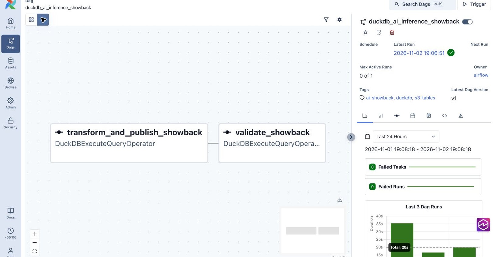
See validate_showback.sql in the sample bundle for the complete validation SQL. In the Airflow user interface, unpause duckdb_ai_inference_showback and trigger the DAG manually. The graph should show transform_and_publish_showback running before validate_showback.
The validation checks the row count and logical-key uniqueness of both summary tables in addition to the detailed-table manifest, event-ID uniqueness, and allocation-state checks. These assertions make an unchanged-input rerun fail if it creates duplicate summary rows.
Figure 2: The Airflow DAG runs transformation and publication before validation
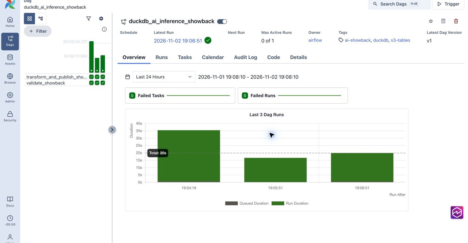
We tested the walkthrough on a new mw1.small Amazon MWAA Provisioned environment in the Canada (Central) Region. The environment had no requirements or plugins file. In the representative run, the pipeline processed 303,543 source rows, removed 3,543 later-arriving duplicates, and published 300,000 unique events. The transform-and-publish task completed in about 11 seconds, and validation completed in about 6 seconds. These measurements describe this test run. Performance varies with worker capacity, data layout, and concurrent workloads.
Figure 3: The representative run and two unchanged-input reruns completed successfully
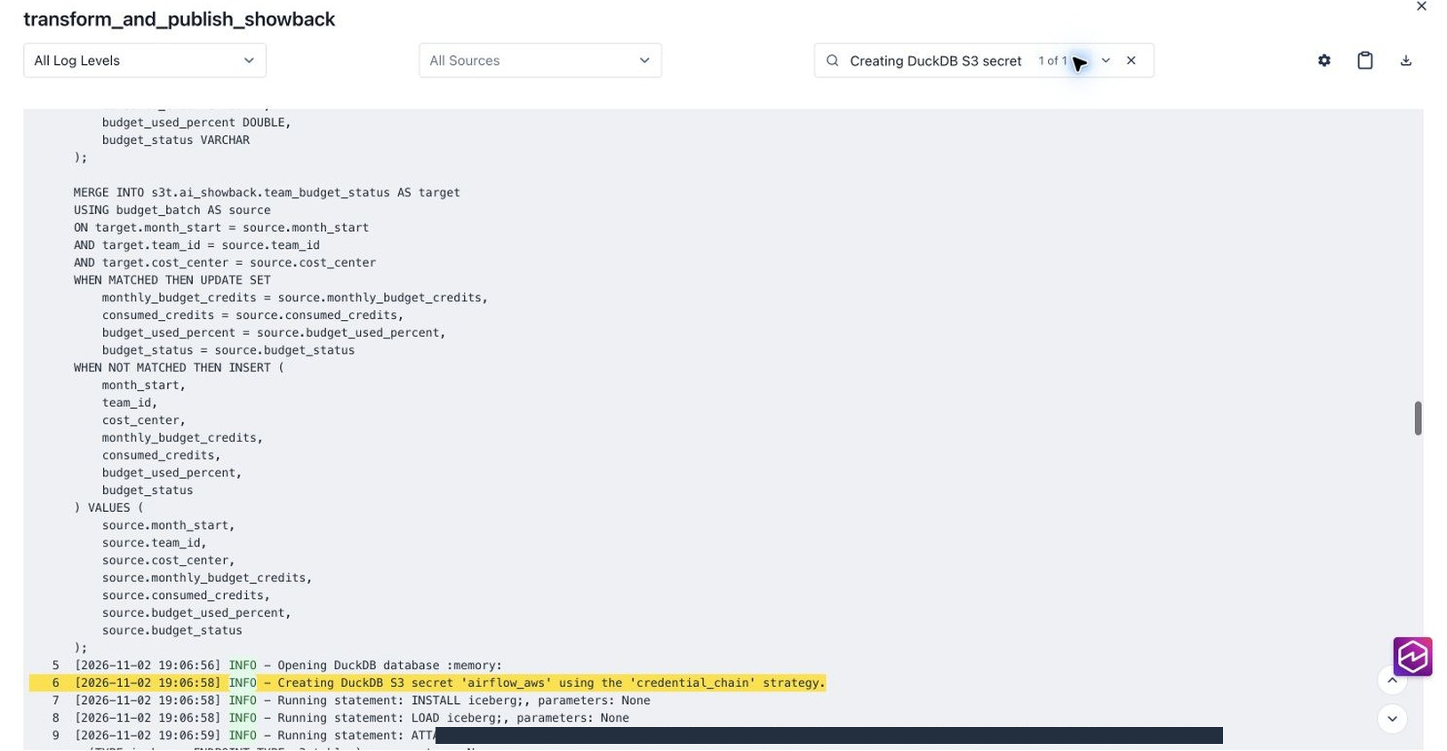
Review the transform-and-publish task log to confirm that DuckDB loaded the required extensions, read the inputs, and committed the Iceberg tables.
Figure 4: The AWS aware hook creates the DuckDB S3 secret from temporary Amazon MWAA execution-role credentials before publication
The validation task confirmed unique event IDs, a detailed row count matching the generator manifest, all expected allocation states, and unique logical keys in both summary tables. The result contained 272,728 allocated events, 3,683 events missing a rate, 5,522 events missing ownership, and 18,067 non-success events. The summary tables contained 8,949 daily application rows and 9 team budget rows.
Figure 5: The validation task reports PASS for uniqueness, row count, and allocation coverage
Trigger the DAG twice more without changing the source files. In our test, all three runs retained 300,000 unique events, 8,949 daily application rows, 9 team budget rows, the same allocation counts, and zero duplicate logical keys. This demonstrates repeatability for unchanged input, but does not establish recovery from partial failures or concurrent external writes.
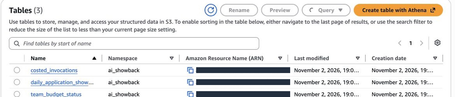
The pipeline published a detailed costed_invocations table and two summary tables, daily_application_showback and team_budget_status, in the ai_showback namespace.
Figure 6: Amazon S3 Tables contains the detailed output and two summary tables
When you run DuckDB with Amazon MWAA, each task runs in an Amazon MWAA worker container whose CPU and memory depend on the environment class. Because Amazon MWAA uses the Celery executor, a single worker can run multiple Airflow tasks concurrently. Keep the following in mind:
Worker capacity: Set the DuckDB memory limit, thread count, and temporary spill space, then test with representative data. Joins, sorting, and data skew can affect peak resource use more than compressed input size alone.
Concurrency: Concurrent tasks on a worker share its CPU and memory, and each DuckDB task can also use multiple threads. Use Airflow pools and max_active_runs to limit how many DuckDB tasks run together and to prevent overlapping writes to the same tables.
Processing boundary: Use this pattern when SQL processing completes reliably within one worker. If a step needs horizontal scaling, high write concurrency, or more resources than one worker provides, run it with AWS Glue or Amazon EMR. Amazon MWAA can continue to orchestrate it.
To avoid ongoing charges, pause the DAG and remove its file from the Amazon MWAA DAG folder. Delete the synthetic source data and drop the tutorial Iceberg tables. Remove the table bucket, source bucket, and Amazon MWAA environment only if you created them exclusively for this walkthrough. Remove any tutorial-specific permissions that are no longer needed.
Conclusion
In this post, you used Amazon MWAA to orchestrate an embedded DuckDB analytics pipeline. DuckDB ran inside the Airflow tasks to transform Parquet data from Amazon S3, publish the results as Apache Iceberg tables in Amazon S3 Tables, and validate the output. The DAG defined the task dependencies, while Amazon MWAA ran and monitored the tasks.
This pattern suits bounded, SQL-oriented transformations that fit within one worker. Start with representative data, set DuckDB memory and thread limits, and test retries, concurrency, and multi-table write behavior. If a task outgrows one worker, Amazon MWAA can continue orchestrating the workflow while a distributed service performs that step.
We thank Kamen Sharlandjiev (Principal Specialist Solutions Architect) and Aritra Ghosh (Senior Product Manager) for their contributions to this post.
Today, we are announcing the general availability of Amazon OpenSearch Memory, a new capability built on Amazon OpenSearch Serverless for adding persistent memory to AI agents. OpenSearch Memory stores agent interactions as searchable events, derives useful memories, and retrieves relevant context across sessions. You can give agents long-term memory without provisioning infrastructure or building separate extraction, indexing, consolidation, and retrieval systems.
AI agents need memory when an interaction depends on information from an earlier session. A support agent might recall a customer’s open case and product configuration, a coding agent needs repository conventions and prior decisions, and a personal assistant keeps a user’s preferences. An agent that restarts or hands off a conversation also needs the exact turns that came before. Passing the complete conversation history to the model becomes slower and more expensive as that history grows, and the relevant information can be difficult to find.
Building a memory system requires more than storing transcripts. You must capture events, extract facts and summaries, generate embeddings, reconcile new information with existing memories, retrieve the right context, isolate data, and enforce retention and deletion policies. You must also operate the infrastructure and evaluate whether the retrieved memories improve agent responses.
OpenSearch Memory manages these functions as one serverless capability. Your application writes conversation events after each turn and searches for relevant memories and events before generating a response. OpenSearch Memory stores the original events verbatim, makes them searchable within seconds, and asynchronously derives structured memories. It handles extraction, embedding, indexing, consolidation, retrieval, data isolation, and retention.
How OpenSearch Memory works
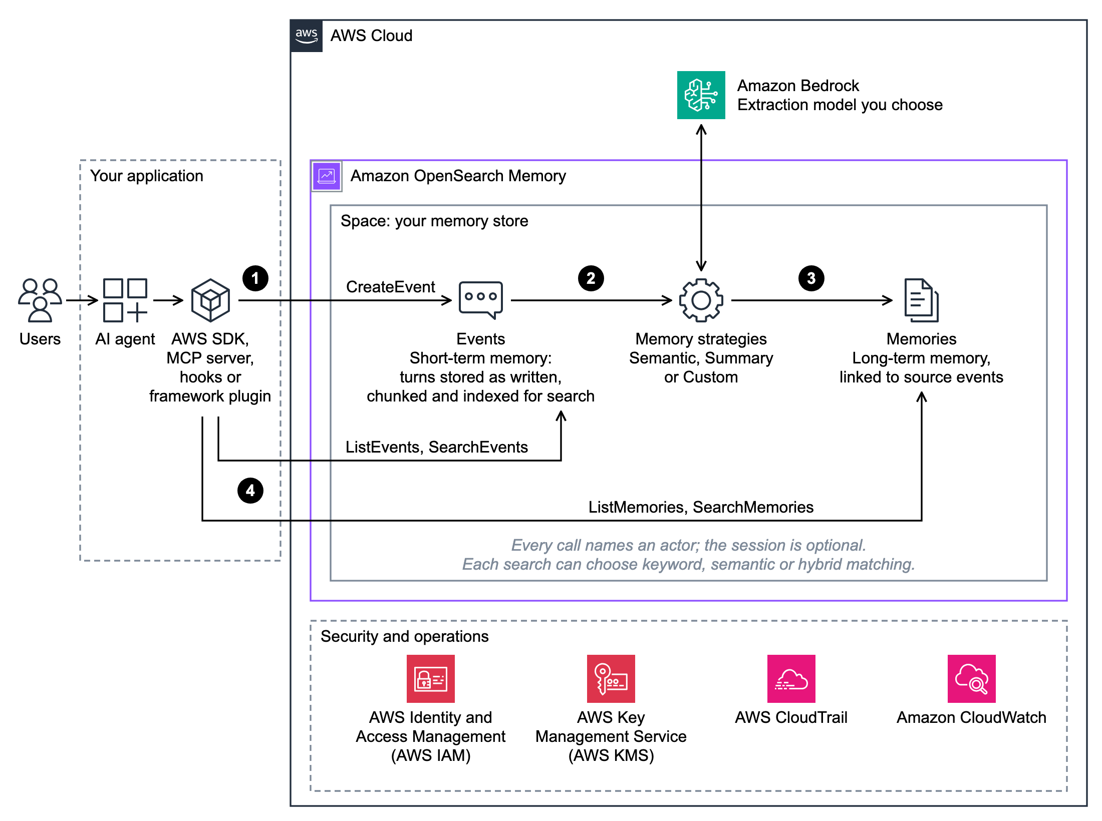
The architecture has two boundaries: your application and OpenSearch Memory. Your AI agent connects through an AWS SDK, an AWS Model Context Protocol (MCP) server, a hook, or a supported framework integration. The following diagram shows how your application writes events to a space, how OpenSearch Memory derives memories using an Amazon Bedrock model that you choose, and how your application retrieves context. Extraction and embedding costs are included in OpenSearch Memory pricing. For details, see Amazon OpenSearch Service pricing.
Figure 1: How an application writes events to an Amazon OpenSearch Memory space, derives memories with an Amazon Bedrock model, and retrieves context
OpenSearch Memory organizes data in a space, the AWS resource that serves as a memory store. A space contains the following:
Events, which are the original interactions written by your application.
Memories, which are facts, preferences, and summaries derived from those events.
Every request names an actor, the end user the data belongs to. An optional session ID groups events from one conversation. A condition key on the agent’s AWS Identity and Access Management (IAM) role can limit which actors the agent can act for, and event reads and searches can be limited to one session. Data in a space is encrypted with AWS Key Management Service (AWS KMS), and you can use your own customer managed key. AWS CloudTrail logs API calls to a space, and Amazon CloudWatch reports its metrics.
The write and retrieval paths operate independently:
After each interaction, your application writes the conversation turn to a space as an event. OpenSearch Memory stores the event verbatim (CreateEvent) and indexes it for keyword, semantic, and hybrid search. Events are available to read immediately and become searchable within seconds.
In the background, the memory strategies configured on the space extract memories from these events.
OpenSearch Memory compares each new memory with the existing ones and adds, updates, or skips it, so stored memories stay current.
Before the agent responds, your application retrieves context: memories about the user from past conversations, the exact turns of the current or earlier conversations, or both. Your application adds the retrieved context to the model’s prompt.
Benchmarking OpenSearch Memory with LongMemEval
In this evaluation, the configured OpenSearch Memory workflow gave the answering model about one-twelfth as many input tokens as the full conversation history (about 13,500 compared with 167,000 per question). It preserved most of its answer accuracy: 93.0% compared with 95.2%.
We used LongMemEval-S to evaluate whether a complete memory workflow could help an AI assistant answer questions that depend on earlier conversations. The public benchmark contains 500 questions about information distributed across approximately 50 chat sessions for one user (Wu et al., ICLR 2025). It evaluates the final answers produced using retrieved memories, rather than memory extraction alone.
For this evaluation, we configured the OpenSearch Memory workflow as follows:
We wrote the benchmark conversations to OpenSearch Memory as events.
The space’s default memory strategies, for facts and session summaries, derived and consolidated memories from those events.
For each question, the answering model received the top 30 memories and events from hybrid search.
Claude Opus 5.5 answered each question from those results and, in a separate call, graded each answer against the benchmark’s reference answer.
Claude Haiku 5.5 extracted memories, and Amazon Titan Text Embeddings created the embeddings. Each result comes from one run, with a 95% confidence range of 2 to 3 points either way. To limit grading bias, Opus 5.5 graded each answer in a separate call that saw only the question, the reference answer, and the answer.
We compared the OpenSearch Memory workflow with two baselines: retrieving raw conversation turns with BM25 keyword search, and supplying the complete conversation history to the answering model. Claude Opus 5.5 answered and graded all three.
Context supplied to the answering model
What the comparison measures
Answer accuracy
Context tokens per question
OpenSearch Memory: top 30 results from memories and events
The configured extraction, consolidation, and hybrid retrieval workflow
93.0%
Approximately 13,500
BM25: top 30 raw conversation turns
Keyword retrieval without memory extraction or consolidation
88.6%
Approximately 22,700
Full conversation history
Answering with all conversation turns
95.2%
Approximately 167,000
For agents with long-running conversations, this approach can reduce model input costs and preserve room in the context window without discarding information from earlier sessions. The workflow also scored 4.4 percentage points higher than BM25 retrieval over raw conversation turns. These results reflect the tested setup, including its memory strategies, models, and retrieval settings, and do not represent every possible OpenSearch Memory configuration.
Getting started with Amazon OpenSearch Memory
You can create your first space from the Amazon OpenSearch Service console or the AWS SDK. The following sections walk through both.
Launch OpenSearch Memory from the console
You can create a space and inspect its events and memories in the Amazon OpenSearch Service console. The following video shows the steps.
In the Amazon OpenSearch Service console, under Memory, choose Spaces, and then choose Create Space.
Choose Easy create, enter a space name, and choose Create Space. Easy create adds a Semantic and a Summary strategy and uses service defaults for encryption and expiry. Choose Standard create to set these yourself.
Wait for the status to change from Creating to Active. The Memory strategies tab shows the strategies on the space.
After your agent writes events, open the Events tab and enter an actor ID to see each conversation. The Memories tab shows the memories extracted from those events.
Walkthrough with the AWS SDK
This walkthrough adds memory to a customer support agent. The agent needs to remember account details, prior case history, and user preferences across sessions.
Prerequisites
To follow this walkthrough, you need the following:
An AWS account with permissions to create and use OpenSearch Memory spaces.
Python 3.10 or later and the AWS SDK for Python (Boto3) 1.44.4 or later.
One of the supported AWS Regions: US East (N. Virginia), US West (Oregon), Asia Pacific (Tokyo), or Europe (Frankfurt).
1. Create a space
You start by creating a space for the support agent. This is a one-time setup. The space defines what the service extracts, how long it keeps data, and how it encrypts it.
import boto3

REGION = "us-east-1"
osm = boto3.client("opensearchmemory", region_name=REGION)

space = osm.create_space(
    name="customer-support-agent",
    memoryStrategies=[
        {"type": "SEMANTIC", "name": "facts-and-preferences"},
        {"type": "SUMMARY", "name": "session-summaries"},
    ],
    eventExpiryDays=90,       # keep raw events for 90 days (1-365)
    memoryExpiryDays=365,     # keep memories for 1 year (0 = never expire)
    # extractionModelId="anthropic.claude-opus-5-5",  # optional; Claude Haiku 5.5 by default
    # encryptionConfiguration={"kmsKeyArn": "..."},  # optional customer managed AWS KMS key; can only be set here
)
space_id = space["spaceId"]

# The space starts in CREATING. The waiter returns once it is ACTIVE and raises if it reaches FAILED.
osm.get_waiter("space_active").wait(spaceId=space_id)
2. Write events after each turn
After each agent turn, you write an event. The call returns after the event is stored, and extraction runs in the background.
def conversational(turns):
    """Build a CreateEvent payload from [(role, text), ...]."""
    return {"conversational": {"unified": {"source": {"object": {
        "messages": [{"role": role, "content": {"text": text}} for role, text in turns]
    }}}}}

event = osm.create_event(
    spaceId=space_id,
    actorId="user-42",           # the end user
    sessionId="session-007",     # one stable ID per conversation
    payload=conversational([
        ("USER", "I'm calling again about Case #78234. It's still not resolved."),
        ("ASSISTANT", "I've escalated Case #78234 to billing. Your reference is ESC-5521, and billing will reply within 48 hours."),
    ]),
    metadata={"channel": "phone"},   # optional metadata, copied onto derived memories
)
event_id = event["event"]["eventId"]
Extraction freshness: Memories appear after the service processes the events in the background, so for a brand-new user, a memory search (step 3) can return nothing at first. Events don’t wait. They are readable as soon as the write returns and searchable within seconds. An agent that restarts or hands off the conversation can resume the session from its events right away. Use ListEvents to find the session’s recent events, and BatchGetEvent or GetEvent to read them. By default, ListEvents returns a session’s events newest first, so the following slice reads the most recent turns. Pass the sort parameter to return them oldest first instead.
# Resume the session: read its latest turns
recent = osm.list_events(spaceId=space_id, actorId="user-42", sessionId="session-007")
turns = osm.batch_get_event(
    spaceId=space_id,
    eventIds=[e["eventId"] for e in recent["events"][:10]],   # up to 10 IDs per call
)
Writing memories directly: You can also write a memory directly with CreateMemory. Use it to import what you already know, such as preferences from an existing customer relationship management (CRM) system, or to let the agent save its own findings. The service embeds and stores the memory under the strategy that you name.
# Import a preference from your CRM
osm.create_memory(
    spaceId=space_id,
    name="facts-and-preferences",   # a strategy name declared on the space
    actorId="user-42",
    content="The user prefers to be contacted by email.",
)

# Let the agent save its own finding about this user's case
osm.create_memory(
    spaceId=space_id,
    name="facts-and-preferences",
    actorId="user-42",
    content="Case #78234 is waiting on a manager approval code for the annual-plan refund.",
    metadata={"writtenBy": "support-agent"},   # marks agent-written memories so you can review or correct them later
)
The added metadata here keeps a record of which memories the agent wrote, so you can audit them later. Agent-written memories persist across sessions and feed later prompts, so review or correct them, for example by filtering on the writtenBy metadata, before you rely on them.
3. Search memories before each response
Before generating a response, you search the space for memories about this user and add them to the agent’s system prompt.
results = osm.search_memories(
    spaceId=space_id,
    actorId="user-42",            # every search is scoped to one actor
    query={
        "hybrid": {
            "queries": [
                {"match": {"memory_text": "Case #78234 open cases and account status"}},
                {"neural": {"memory_vector": {
                    "query_text": "open cases and account status", "k": 10}}},
            ]
        }
    },
    maxResults=10,
)

context = "\n".join(m["content"] for m in results["memories"])
# Add `context` to the agent's system prompt
In this support scenario, the keyword half of the query surfaces the exact case number from a prior session. The semantic half retrieves related context, such as the user’s preferred contact method and what the case is waiting on. The user doesn’t need to repeat themselves. Each turn adds two calls to your agent loop: one search before it responds, one write after.
Each result also carries sourceEventIds, the events the memory was derived from, so you can trace any fact back to the conversation that produced it.
Search the conversation itself: Memories capture what a conversation means. Events keep the conversation itself: every turn, verbatim, with who said it. To find an exact phrase, such as a commitment the agent made earlier in the conversation, search the events:
hits = osm.search_events(
    spaceId=space_id,
    actorId="user-42",
    sessionIds=["session-007"],   # optional: search only this conversation
    query={"match_phrase": {"text": "reply within 48 hours"}},
    maxResults=5,
)
snippets = [e["matchedContent"] for e in hits["events"]]   # the exact turns, with who said what
4. Let consolidation keep facts current
Users’ facts change. Consolidation handles the change without extra code.
# Session 1
osm.create_event(spaceId=space_id, actorId="user-42", sessionId="s-001",
    payload=conversational([("USER", "I'm based in New York.")]))

# Session 10, weeks later, after the user moves
osm.create_event(spaceId=space_id, actorId="user-42", sessionId="s-010",
    payload=conversational([("USER", "I just relocated to Seattle last week.")]))

# Once session 10 is processed, SearchMemories returns one updated memory,
# "The user was based in New York and relocated to Seattle ...",
# instead of keeping the old and new facts side by side.
Consolidation is on by default for every strategy. To keep an append-only history instead, set consolidationEnabled to False in the strategy’s configuration:
Amazon OpenSearch Memory is generally available today in four AWS Regions: US East (N. Virginia), US West (Oregon), Asia Pacific (Tokyo), and Europe (Frankfurt). For pricing, including storage, retrieval, and extraction, see Amazon OpenSearch Service pricing. To start building, use the AWS SDK, the MCP server, or the OpenSearch Memory skills for Kiro, Claude Code, and Codex.
With OpenSearch Memory, your agents keep context across sessions without you building or operating a memory system.
To learn more, see OpenSearch Memory in the Amazon OpenSearch Service Developer Guide.
Aderant, a global provider of business management software for the legal industry, modernized the data pipeline powering its Stridyn analytics tool using Apache Iceberg, AWS Lambda, and AWS Glue. The new architecture delivers near real-time data availability for 700 client environments across 266 source tables. It replaces a batch-oriented pipeline that took 15 minutes per processing cycle with an event-driven system that processes change data capture (CDC) events in single-digit seconds.
In this post, we share how Aderant redesigned its multilayer data pipeline using a medallion architecture (bronze, silver, and gold layers) built on Apache Iceberg tables. This approach achieved 10–26x faster query performance and a 77 percent cost reduction compared to alternative approaches. We include architecture details, performance benchmarks, and the decision framework so that analytics teams managing multi-tenant SaaS tools can apply the same pattern.
The challenge: Batch processing limiting analytics freshness
Aderant’s Stridyn analytics application serves 700 client environments running Expert Sierra, its cloud-based legal practice management solution. The tool processes data from 266 source tables in Microsoft SQL Server databases, delivering financial reports, billing analytics, and operational dashboards to law firms globally.
The existing pipeline faced several challenges:
Slow processing times. A full data processing cycle took approximately 15 minutes, with batch job overhead adding latency before data transformation could begin.
Limited real-time data availability. Clients experienced delays between operational changes and analytics visibility, impacting time-sensitive billing and matter management decisions.
Performance issues with complex queries. Reports involving window functions, joins across multiple fact tables, and common table expressions (CTEs) suffered from slow response times when querying external tables through Amazon Redshift Spectrum.
Scalability constraints. The architecture struggled to handle custom data, schema changes, and a growing volume of CDC events that already reached 380 million per month across all tenants.
The catalyst for modernization came from Aderant’s commitment to delivering near real-time data availability, making sure data is accessible within minutes from source to target without changing the end-user experience.
The solution: Event-driven medallion architecture with Apache Iceberg
Aderant built a new data pipeline using a medallion architecture with three distinct layers (bronze, silver, and gold), all built on Apache Iceberg tables stored in Amazon Simple Storage Service (Amazon S3). The architecture uses AWS Lambda for event-driven CDC processing, AWS Glue for transformations, and Amazon Redshift for the final analytics serving layer.
How it works: The lifecycle of a data change
The following steps describe what happens when a record changes in a client’s source database.
CDC capture and delivery.AWS Database Migration Service (AWS DMS) captures changes from Microsoft SQL Server databases and writes Parquet files to an S3 landing zone, organized by table and tenant.
Event-driven ingestion (raw to bronze). An S3 event notification triggers an Amazon Simple Queue Service (Amazon SQS) message, which invokes a Lambda function that processes the CDC payload and writes to bronze-layer Iceberg tables in single-digit seconds per event.
Bronze-to-silver transformation. AWS Glue jobs read incremental data from bronze tables using Amazon DynamoDB-based watermarking, apply normalization and deduplication through Iceberg MERGE operations, and produce current-state silver tables with ACID adherence.
Silver-to-gold aggregation. The gold layer uses two approaches based on table complexity: incremental AWS Glue jobs for 77 standard gold tables, and materialized views with Iceberg snapshot comparison for 34 tables with complex query patterns that cannot be easily incrementalized.
Gold-to-Amazon Redshift delivery. Delta changesets from materialized view snapshots are written to native Amazon Redshift tables, where columnar storage, zone maps, and sort keys deliver sub-100-millisecond query performance for end-user dashboards.
Why Apache Iceberg
Aderant chose Apache Iceberg as the table format across all pipeline layers for three reasons.
ACID transactions for concurrent operations. With 700 tenants generating CDC events simultaneously, Iceberg’s snapshot isolation helps prevent conflicts when multiple Lambda functions write to the same tables concurrently.
Time travel and snapshot comparison. For the 34 complex gold tables, Iceberg’s snapshot metadata identifies deltas without manual watermarking. The system compares consecutive snapshots to determine exactly which rows changed, then writes only those deltas to Amazon Redshift.
Schema evolution without pipeline disruption. As Aderant onboards new data sources and clients customize their schemas, Iceberg handles column additions and type changes without requiring full table rebuilds.
Why AWS Lambda for CDC processing
After evaluating three architectural approaches, the team chose Lambda based on cost, latency, and operational simplicity. The Docker container image deployment model (using Amazon Elastic Container Registry) accommodates the large library dependencies required for Iceberg operations, including PyIceberg and pandas. The pay-per-invocation model also aligns naturally with CDC workloads, where event volume fluctuates throughout the day, scaling to zero during quiet periods and handling 10x seasonal spikes without pre-provisioned capacity.
Architecture
The following diagram illustrates the end-to-end data flow from source databases through the medallion layers to the analytics serving layer.
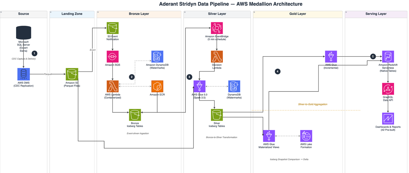
Figure 1: End-to-end data flow through the medallion architecture, from source databases to the Amazon Redshift serving layer
The pipeline begins at the source layer, where AWS DMS replicates CDC events from Microsoft SQL Server databases into an Amazon S3 landing zone as Parquet files. When new files arrive, Amazon S3 Event Notifications publish messages to an Amazon SQS queue. The queue serves as a buffer to handle burst traffic and provides dead-letter queue capabilities for failed events.
AWS Lambda functions, deployed as Docker containers through Amazon Elastic Container Registry (Amazon ECR), consume messages from the SQS queue and write to bronze-layer Iceberg tables in Amazon S3. These Lambda functions use the PyIceberg library to perform ACID-aligned writes, and Amazon DynamoDB stores watermark state to track processing progress and help prevent duplicate writes. The AWS Glue Data Catalog registers Iceberg table metadata across the bronze, silver, and gold layers.
Amazon EventBridge triggers the next stage on a 5-minute schedule, invoking a decision Lambda function that checks whether bronze-to-silver AWS Glue jobs should run based on data availability. When new data is present, AWS Glue 5.0 jobs (running Apache Spark 3.5 on Python 3.11) read incrementally from bronze tables. These jobs apply MERGE operations for deduplication and normalization, then write clean records to silver-layer Iceberg tables. DynamoDB watermarks make sure each AWS Glue job processes only new data since its last successful run.
The silver-to-gold transition follows two paths. For the 77 standard gold tables, Amazon EventBridge detects the completion of bronze-to-silver jobs and triggers a second decision Lambda. That Lambda launches incremental AWS Glue jobs that write directly to Amazon Redshift native tables through the Amazon Redshift Data API. For the 34 complex gold tables, AWS Glue materialized views perform the transformation in SQL. A separate AWS Glue job compares Iceberg snapshots to extract only the changed rows and writes those delta changesets to Amazon Redshift native tables.
Amazon Redshift Serverless serves as the final analytics layer, where native tables with columnar storage, zone maps, and sort keys deliver sub-100-millisecond query latency. A GraphQL Data API layer sits between Amazon Redshift and the end-user dashboards, serving 42 pre-built reports including financial statements, billing analytics, and firm overview dashboards.
Amazon CloudWatch provides end-to-end observability across pipeline components, with custom metrics tracking processing latency, error rates, and throughput per tenant. AWS Identity and Access Management (IAM) enforces least-privilege access, and S3 data is encrypted using AWS Key Management Service (AWS KMS) with server-side encryption. The entire infrastructure is defined in Terraform and deployed through GitHub Actions continuous integration and continuous delivery (CI/CD) pipelines.
Materialized views: Solving the complex query problem
A notable aspect of the architecture is how Aderant handles the 34 gold tables that involve complex SQL patterns: LAG/window functions, joins across multiple fact tables, UNIONs with aggregations, and CTEs.
For these tables, traditional incremental processing would require redesigning each query’s logic. Instead, the team uses AWS Glue materialized views as an intermediate step:
Create materialized views using standard Spark SQL (CREATE MATERIALIZED VIEW AS SELECT ...) against silver-layer Iceberg tables.
Automatic change tracking through Apache Iceberg, which monitors source table changes without manual watermarking.
Scheduled refresh every 2–5 minutes through AWS Glue jobs (bypassing the 1-hour minimum for automatic refresh).
Delta extraction by comparing Iceberg snapshots between refreshes.
Write to Amazon Redshift only the changed rows as native table updates.
This approach alleviates the need to rewrite complex analytical queries while still achieving incremental processing. The materialized view handles the computational complexity, and Iceberg’s snapshot comparison identifies what changed.
Quantifiable results
The architecture improvements delivered measurable gains across three dimensions: query performance, pipeline latency, and infrastructure cost.
Query performance
The team benchmarked 16 analytical queries, ranging from simple aggregations to complex pivots over 9 million rows, comparing Amazon Redshift native tables against external tables queried through Amazon Redshift Spectrum. Across all query types, native tables delivered 10–26x faster response times, consistently returning results in under 100 milliseconds regardless of dataset size. The largest improvement came on smaller, frequently accessed datasets (25.8x speedup), while complex pivot queries with window functions still achieved a 13.7x improvement. These benchmarks were conducted on Amazon Redshift Serverless at 16 RPU, meaning provisioned clusters with dedicated compute and persistent caching would perform even better.
The team also validated Amazon S3 Express One Zone for workloads that remain on S3-based Iceberg tables without Amazon Redshift. It reduced query latency by 31–78 percent compared to Amazon S3 Standard, with the greatest gains on complex queries involving multiple table scans.
Pipeline latency
The largest operational improvement is end-to-end processing time. The previous pipeline required approximately 15 minutes per full processing cycle. The new event-driven ingestion layer processes CDC events without batch job overhead. CDC events now flow from source database to bronze-layer Iceberg tables in single-digit seconds. Gold layer refreshes complete in under 5 minutes for initial loads and under 1 minute for incremental updates. The system sustains throughput of 186,000+ events per second across all 266 tables and 700 tenants.
Infrastructure cost
By choosing Lambda-based event processing over streaming alternatives, Aderant achieved a 77 percent reduction in pipeline compute costs. The serverless, pay-per-invocation model scales to zero during quiet periods and handles 10x seasonal spikes without pre-provisioned capacity, keeping costs proportional to actual data volume rather than reserved infrastructure.
In production: Multi-tenant operations
The architecture runs in production today, processing data for 700 client environments across 266 source tables. Three aspects of the implementation stand out.
Tenant isolation with shared infrastructure. Each tenant’s CDC events flow through the same Lambda functions and AWS Glue jobs, but Iceberg’s partition-by-tenant structure maintains data isolation. Configuration files drive per-tenant behavior without code changes.
Graceful handling of complex reports. The Expert Bill Report, one of Aderant’s most complex analytical outputs involving multiple dimension tables and fact aggregations, processes 900,000 records in approximately 5 minutes for initial load, with subsequent incremental runs handling only changed records in seconds.
Self-healing watermark management. DynamoDB-based watermarks track the last processed timestamp per table per tenant. If a Lambda function fails, the watermark remains unchanged, and the next invocation reprocesses from the correct point, providing exactly-once semantics without complex distributed transaction logic.
Looking ahead
Aderant plans to continue expanding the tool’s capabilities.
Streaming analytics for high-volume tenants. The Lambda-based architecture supports a hybrid model where tenants with the highest event volumes can migrate to Amazon Kinesis streaming for sub-second latency, while standard tenants remain on the cost-effective Lambda path.
AI-powered analytics. Integration with Amazon Bedrock for natural language querying of the gold layer, so law firm users can ask questions about their billing and matter data conversationally.
Automated data quality. Expanding the validation framework to continuously monitor data consistency between pipeline layers, with automated alerting when discrepancies are detected.
Conclusion
Aderant’s journey from batch-oriented data processing to an event-driven, Iceberg-based pipeline demonstrates what is possible when you combine modern open table formats with serverless compute. The new architecture processes CDC events in single-digit seconds instead of 15-minute batch cycles. It delivers 10–26x faster query performance through native Amazon Redshift tables and reduces infrastructure costs by 77 percent compared to streaming alternatives.
The key insight is that not every table needs the same processing strategy. Aderant uses incremental AWS Glue jobs for straightforward tables and materialized views with Iceberg snapshot comparison for complex analytical patterns. This approach delivers near real-time freshness across all 111 gold tables without rewriting complex SQL logic.
For analytics teams managing multi-tenant SaaS tools, Aderant’s experience shows the value of Apache Iceberg. Its ACID alignment, time-travel capabilities, and schema evolution support make it a strong foundation for production data pipelines at scale.
This post is co-authored with Tunde Fowora, Principal Architect at United Airlines. United Airlines, headquartered in Chicago, IL, United States, is the world’s largest airline based on revenue passenger miles, according to United Airlines.
In this post, we explore how United Airlines adopted Apache Iceberg for large-scale data processing while managing near-real-time data synchronization from transactional databases.
United Airlines needed to replicate frequently changing reference data in near-real-time from an operational Amazon Aurora MySQL-Compatible Edition (Aurora MySQL) database to a new cloud-native analytics system built on Apache Iceberg, during a multi-year modernization. Until that migration completed, changes in the source database still had to reach analysts and downstream systems within minutes. The legacy batch process could not keep pace, so teams analyzed market patterns on stale data, which delayed business decisions.
To meet that need, United Airlines built a near-real-time Change Data Capture (CDC) pipeline using Amazon Kinesis Data Streams (Kinesis Data Streams), AWS Lambda (Lambda), Amazon Data Firehose (Firehose), and Apache Iceberg on Amazon Simple Storage Service (Amazon S3) to ingest database change events emitted from a database CDC engine. At United, database CDC is implemented using the AWS Database Migration Service (AWS DMS) CDC engine. Moving to Iceberg removed the scalability limits of the legacy SQL databases. Queries scanning more than 10 million rows no longer hit those bottlenecks, and several hundred business analysts could run complex queries across a broader data domain. In United’s testing, average query latency improved 5x. Because those queries run inside downstream AWS Glue extract, transform, and load (ETL) jobs, total job processing time dropped 2x while reducing billed AWS Glue run time. Once landed in Iceberg tables, the data is queryable from AWS Glue, Amazon Redshift, and Amazon Athena. Any Iceberg-compatible engine can access the data.
The streaming layer is what keeps this pattern straightforward to operate. Amazon Data Firehose reads the change events from Kinesis Data Streams, writes them to the Iceberg table as Parquet files, applies each insert, update, and delete, and commits a new table snapshot. You don’t build a separate application or manage servers for that delivery step. Kinesis Data Streams can also run in on-demand mode, which scales capacity automatically as change volume grows.
In this post, you’ll learn how to reproduce this approach for your own high-volume CDC requirements, including AWS CloudFormation automation, Amazon CloudWatch monitoring, and performance trade-offs. This architecture is valuable for any industry that needs near-real-time analytics on transactional data, such as financial services, retail inventory management, and travel and hospitality revenue optimization.
Note on this walkthrough: The following is grounded in United Airlines’ pre-production implementation but is intentionally simplified so you can reproduce it quickly. Read these points before you begin:
CDC engine: United Airlines runs this pipeline on standard (provisioned) AWS DMS. Use any CDC engine that can write change events to Kinesis Data Streams and supports your source database. For simplicity, this walkthrough and the accompanying template use AWS DMS Serverless, which removes replication-instance sizing and management. In this walkthrough, AWS DMS writes each change to Kinesis Data Streams as a record that holds the row data plus metadata such as the schema name, table name, and operation type. The downstream pipeline, from Kinesis Data Streams through Iceberg, stays the same whatever engine you pick. The AWS Lambda transform is the one engine-specific piece: it parses the CDC engine’s record format and emits the destination database, table, and operation that Firehose needs to route each record (Route incoming records to different Iceberg tables), so you rewrite it when you change engines.
Query engine: At United Airlines, analysts primarily use Amazon Redshift Serverless. This walkthrough uses only Amazon Athena for validation, to keep the steps focused. Because the data lands in open Apache Iceberg tables cataloged in the AWS Glue Data Catalog, the same data layer is queryable from multiple engines, including AWS Glue, Amazon Redshift, and Amazon Athena.
Scope of the template: The provided AWS CloudFormation template is a simplified, representative view of what United Airlines built, not the complete production solution. Its purpose is to give you a working starting point that you can adapt and make your own. It is not intended to cover every automation, hardening, or operational requirement.
Operational settings: The template uses demo values, not production-tuned ones. It logs at debug level in the CDC engine and uses four provisioned Kinesis shards with 24-hour retention that aren’t sized for a specific throughput. For variable workloads, consider on-demand capacity mode. The Firehose Iceberg destination uses a 1 MB, 3-second buffer and a 300-second retry duration so results appear quickly in the demo. A short buffer commits a snapshot and delete files every few seconds. Before production use, review buffering, error handling, and monitoring in Set up the Firehose stream, Handle failure in data transformation, and Considerations and limitations for Apache Iceberg tables.
Single-table scope: The provided template replicates one source table (a single CDC engine selection rule mapped to one Iceberg destination table). Replicating additional tables requires extending the template. Use it at your own discretion.
Schema evolution: Enterprise workloads often need to handle source schema changes made with data definition language (DDL) statements over time. That is not covered by this walkthrough. Firehose handles source schema changes as described in Considerations and limitations for Apache Iceberg tables. If a source record has a new field that isn’t in the table, but all other column names and data types match, Firehose skips the new field. If column names or data types don’t match, Firehose returns an error and sends the record to the S3 error bucket. At United Airlines, schema evolution is handled outside of this architecture pattern, not in the Lambda transform.
Solution walkthrough
The following demonstrates how to implement near-real-time Change Data Capture (CDC) replication from Aurora MySQL to Apache Iceberg using AWS managed services. The solution uses a managed, event-driven architecture. CloudFormation automates the replication pipeline, while you manually configure the source and destination endpoints.
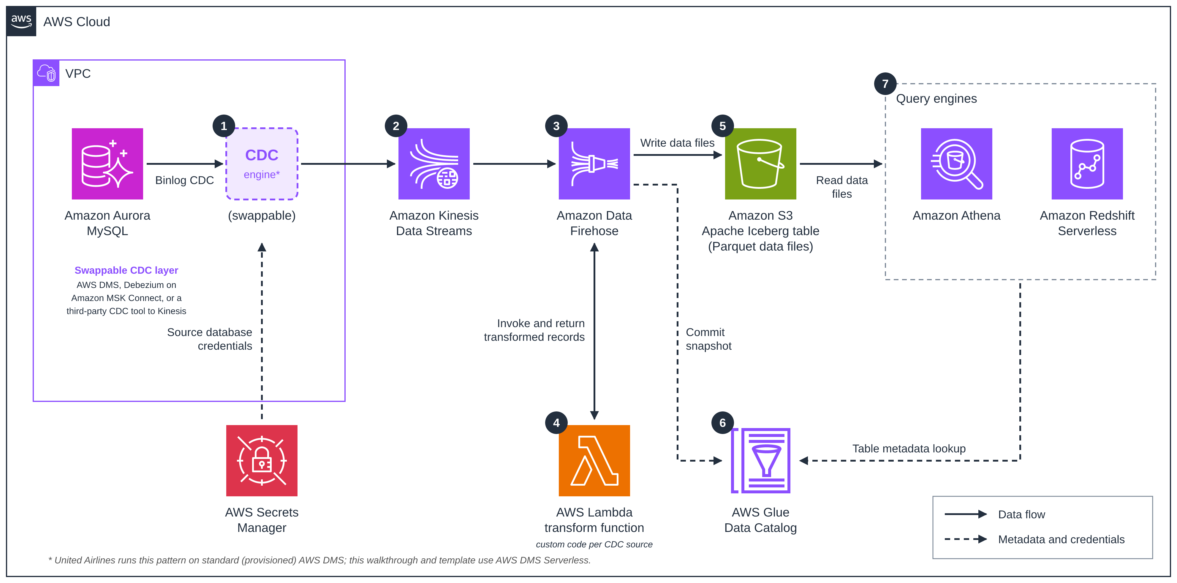
Figure 1 shows the services that make up the near-real-time data replication pipeline:
Figure 1: Architecture overview
Data flow:
The CDC engine captures changes from Aurora MySQL by reading the binary log.
Amazon Kinesis Data Streams receives and buffers the CDC events.
Amazon Data Firehose reads from the stream and batches records.
Firehose invokes an AWS Lambda function, coded for the CDC engine’s record format, to transform each batch.
Firehose writes Parquet data files to the Apache Iceberg table in Amazon S3.
Firehose commits each write as a new Iceberg snapshot, which updates the table’s metadata pointer in the AWS Glue Data Catalog.
Amazon Athena and Amazon Redshift Serverless look up table metadata in the Data Catalog and read the data files from Amazon S3.
The solution architecture can be divided into the following areas:
Data ingestion and streaming
The CDC engine captures changes from an Aurora MySQL database with minimal impact on the source database. Changes stream continuously to Amazon Kinesis Data Streams, which provides durable, scalable real-time data streaming and acts as a buffer between source replication and downstream processing.
Amazon Data Firehose consumes data from Kinesis Data Streams, performing data transformation and batching to prepare data for efficient storage. It reduces infrastructure management overhead while batching records efficiently based on the configured buffer size and interval.
The Firehose buffer interval sets the trade-off between latency and cost. In a low-volume test of about 120 rows, United set the buffer interval to 1 second and saw end-to-end latency as low as 10 seconds. For a large initial load of about 1.5 million rows, United used a 60-second interval in their environment to balance latency, cost, and file size, and the load completed in about 2 hours 22 minutes (about 176 rows per second). United measured these latencies manually against average row throughput.
Processing and storage
An AWS Lambda function processes streaming data in near-real-time. It works in tandem with Amazon Data Firehose (Firehose) to parse CDC event records, extract operation types (INSERT/UPDATE/DELETE), and convert records to the Iceberg-compatible format with the appropriate operation field. Amazon Data Firehose then commits the writes as ACID-compliant (Atomicity, Consistency, Isolation, and Durability) Iceberg snapshots using optimistic concurrency control, updating table metadata automatically. Lambda and Firehose scale with the stream, but the template’s provisioned Kinesis shards and DMS capacity range (1–2 DMS capacity units (DCUs)) are fixed limits.
Firehose applies CDC operations to the Iceberg table using the merge-on-read (MOR) approach: an UPDATE or DELETE is written as a delete file plus, for an update, a new data file, which the query engine merges at read time to resolve the current row state (see Prerequisites to use Apache Iceberg Tables as a destination). This requires the Iceberg table to be format-version 2 and a unique key, which the template sets on the delivery stream.
The template defines no DMS partition-key rule, so DMS uses the schema and table name as the Kinesis partition key and every change for the table lands on one shard, so the other three shards stay idle and throughput is limited to what one shard supports. To spread load and keep per-row order, set the partition key to the table’s primary key in a DMS object-mapping rule (Kinesis as a DMS target). The Lambda function in the template passes each row through and adds the destination table and operation that Firehose uses to insert, update, or delete it.
The self-managed Apache Iceberg tables on Amazon S3 store data in columnar Parquet format, providing durability, scalability, and cost-effective storage. United Airlines pre-creates the Iceberg tables using Amazon Athena, which now hold over 2 TB of data.
Metadata and analytics
AWS Glue Data Catalog serves as the centralized metadata repository, storing Apache Iceberg table metadata, maintaining schema versions and partition information, and supporting schema evolution and governance across the organization.
Amazon Redshift Serverless queries the same Iceberg tables through the AWS Glue Data Catalog. You can reference the table through the auto-mounted awsdatacatalog database (awsdatacatalog.market_db.market_rule) or create an external schema on the Glue database. See Referencing Iceberg tables in Amazon Redshift.
Amazon Athena queries the same tables through the Glue Data Catalog (Query Apache Iceberg tables), with pay-per-query SQL access for ad hoc analysis and data validation and no infrastructure to manage. In our walkthrough test, an UPDATE and a DELETE at the source returned the correct current rows from both Athena and Redshift Serverless.
Solution creation
Prerequisites
Before you begin, make sure you have:
Source database: An Amazon Aurora MySQL cluster with binary logging enabled. Extensibility to other database engines depends on the CDC engine choice. In this example, AWS DMS supports DMS-compatible sources such as PostgreSQL, Oracle, SQL Server, and others. See AWS DMS source documentation. Also, create a secret using AWS Secrets Manager to connect to the database. The secret must contain the Aurora connection details (username, password, host, and port). Note its Amazon Resource Name (ARN), which you will use in Step 2 and as the DmsSourceSecretArn CloudFormation parameter. Create it manually because the Aurora-managed secret omits host and port and will not work with DMS. Also create an IAM access role that DMS can assume to read this secret: give it a trust policy allowing the regional DMS service principal dms..amazonaws.com (for example, dms.us-east-1.amazonaws.com) to assume it, and a permissions policy granting secretsmanager:GetSecretValue on the secret’s ARN. You will attach this role to the source endpoint in Step 2. This walkthrough and template implement the CDC layer with AWS DMS, so the Secrets Manager secret and access role here are DMS-specific. A different CDC engine may authenticate differently and would need corresponding changes.
Network connectivity: A virtual private cloud (VPC) with private subnets where the Aurora MySQL cluster and the replication resources can reach each other, with security group rules allowing access on the database port (3306). Because DMS Serverless runs inside your VPC with no public IP, create a Kinesis Data Streams VPC interface endpoint (com.amazonaws..kinesis-streams) so the replication can reach the Kinesis target. Because the source endpoint authenticates with a Secrets Manager secret, also create a Secrets Manager interface endpoint (com.amazonaws..secretsmanager). Finally, the Aurora cluster’s own security group must allow inbound MySQL (TCP 3306) from the replication’s security group, since the cluster is outside the CloudFormation stack.
AWS permissions: AWS Identity and Access Management (IAM) permissions to create the resources in the stack: the DMS target endpoint and Serverless replication config, Kinesis stream, Lambda function, Firehose delivery stream, CloudWatch log groups, an AWS Key Management Service (AWS KMS) key, and the three IAM service roles (requires CAPABILITY_NAMED_IAM) plus the CloudFormation stack itself. Because the stack creates IAM roles, the deploying identity also needs iam:CreateRole/PutRolePolicy and iam:PassRole so CloudFormation can attach roles to their respective resources during creation.
AWS Command Line Interface (AWS CLI): Installed and configured with appropriate credentials.
Step 1: Configure source database
Assumption: You have an existing Amazon Aurora MySQL cluster. This step is not automated by CloudFormation. This walkthrough was tested on Aurora MySQL version 3.08.0 (compatible with MySQL 8.0).
All SQL in this step (the binlog retention command, the verification query, and the schema and seed statements) runs against your Aurora MySQL database as the admin user, using any MySQL client (or the RDS Data API if the cluster is private). The parameter-group settings in items 1–2 are configured in the RDS console or CLI.
Configure binary logging:
1. In a custom DB cluster parameter group, set binlog_format = ROW, binlog_row_image = FULL, and binlog_checksum = NONE. On Aurora MySQL these come from the cluster parameter group and cannot be set with SET GLOBAL.
2. Associate the parameter group with your cluster if it isn’t already, then reboot the writer instance. binlog_format is a static parameter, so binary logging turns on only after the reboot.
3. Set the binlog retention window on the writer: CALL mysql.rds_set_configuration('binlog retention hours', 24); Set this longer than the longest time the replication might be stopped. Aurora MySQL version 3 allows up to 2,160 hours, or 90 days (Setting up binary log replication). DMS Serverless doesn’t support custom CDC start points (AWS DMS Serverless limitations), so if the replication stays stopped longer than this window, you must restart it with a full reload.
4. Make sure the DMS database user has the REPLICATION CLIENT and REPLICATION SLAVE privileges (see the following note).
Note: For simplicity this walkthrough uses the Aurora admin user for both the Step 1 SQL and the DMS source endpoint, so the “DMS user” in the preceding step is that same admin user, which already holds these privileges. In production, create separate least-privilege users per job. For example, a dedicated DMS replication user with only REPLICATION CLIENT, REPLICATION SLAVE, and SELECT on the source table.
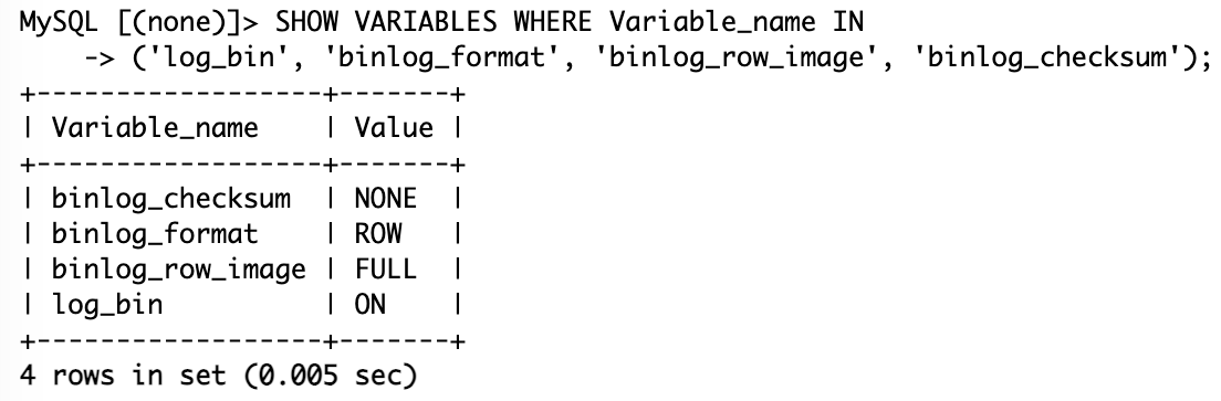
After the reboot, confirm the settings on the writer:
SHOW VARIABLES WHERE Variable_name IN
('log_bin', 'binlog_format', 'binlog_row_image', 'binlog_checksum');
Expect log_bin = ON, binlog_format = ROW, binlog_row_image = FULL, and binlog_checksum = NONE. The log_bin = ON check is the important one as it confirms binary logging is actually active (which requires the reboot to have taken effect), not merely that the format is configured. If log_bin is OFF, confirm the parameter group is associated with the cluster and reboot the writer before continuing.
If your database and tables are not already created in the source database, you may create them using the following SQL commands:
CREATE DATABASE market_db;
USE market_db;

CREATE TABLE market_rule (
    rule_id INT AUTO_INCREMENT PRIMARY KEY,
    name VARCHAR(120) NOT NULL,
    weight INT NOT NULL DEFAULT 0,
    status VARCHAR(10) NOT NULL DEFAULT 'DRAFT',
    effective_from DATETIME(6) NOT NULL,
    market_from VARCHAR(30) NOT NULL,
    market_to VARCHAR(30) NOT NULL,
    created_at DATETIME(6),
    updated_at DATETIME(6)
);
Insert two sample rows so the full-load phase has data to replicate and the Step 6 validation returns results:
Note: For non-MySQL sources, refer to source-specific CDC configuration in the CDC engine documentation (AWS DMS documentation in this example).
Figure 2 shows how to verify the results of Step 1:
Figure 2: Confirmation of binlog activation
Step 2: Create CDC engine source endpoint
Assumption: Your VPC networking and security groups allow the replication resources to reach the Aurora MySQL cluster on port 3306 (see Prerequisites). This step is manual and must be completed before you deploy the CloudFormation stack.
Navigate to AWS DMS Console, then Endpoints, then Create endpoint.
Configure:
Endpoint type: Source endpoint
Endpoint identifier: mysql-source-endpoint
Source engine: Amazon Aurora MySQL
Server name: Your Aurora cluster writer endpoint
Port: 3306 (or appropriate port)
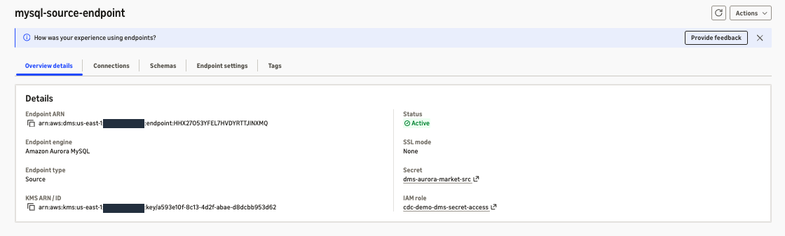
User credentials: reference the Secrets Manager secret and the access role you created in Prerequisites (recommended). Alternatively, you enter the username and password directly on the endpoint instead of using a secret and role.
SSL mode: This walkthrough leaves SSL mode at none, the default for Aurora MySQL endpoints, so the connection between the DMS CDC engine and Aurora isn’t encrypted. For production, set SSL mode to verify-ca or verify-full and attach the Amazon RDS CA certificate (Using SSL with AWS Database Migration Service). On Aurora MySQL version 8.4, require_secure_transport is on by default and rejects SSL mode none, so you must enable SSL.
Figure 3: Confirmation of DMS endpoint connection
Save the endpoint ARN. You’ll need it as the DmsSourceEndpointArn CloudFormation parameter. You’ll also need the ARN of the Secrets Manager secret this endpoint uses (from Prerequisites) as the DmsSourceSecretArn parameter.
Step 3: Set up VPC infrastructure
Assumption: You have an existing VPC with private subnets. These resources are not created by CloudFormation.
First-time DMS setup: If you have never created a DMS subnet group in this account, AWS requires a service role named exactly dms-vpc-role (with a trust policy for dms.amazonaws.com and the AWS-managed policy AmazonDMSVPCManagementRole) so DMS can manage the replication network interfaces. Create it once before the next step. Without it, creating the subnet group fails with an “IAM Role dms-vpc-role is not configured properly” error. The AWS Management Console usually creates this role automatically the first time. If you use the CLI or API, create it explicitly.
Create DMS subnet group:.
DMS Console, then Subnet groups, then Create subnet group
Select at least 2 private subnets in different Availability Zones
Save the subnet group ARN (arn:aws:dms:<region>:<account-id>:subgrp:<subnet-group-name>)
Create security group (for the DMS replication):.
EC2 Console, then Security Groups, then Create security group
Inbound: HTTPS (443) from your VPC CIDR, so the replication can reach the interface endpoints
Outbound: allow HTTPS (443) to AWS services and MySQL (3306) to the Aurora cluster (the default “all traffic” outbound also works)
Save the security group ID
Then, on the Aurora cluster’s security group, add an inbound rule: MySQL (3306) from this DMS security group
Create VPC endpoints (required because the replication runs privately with no internet access):.
VPC Console, then Endpoints, then Create endpoint
Create an interface endpoint for Kinesis Data Streams: service com.amazonaws..kinesis-streams. Select your private subnets. Attach the DMS security group. Enable Enable DNS name (private DNS)
Create an interface endpoint for Secrets Manager: service com.amazonaws..secretsmanager. Same subnets, same security group, private DNS enabled
The interface endpoints show Pending briefly, then Available
Step 4: Create destination infrastructure
Assumption: These resources must exist before CloudFormation deployment. They are not automated. Athena must be set up with a results bucket prior to executing these steps. If the table’s S3 location is registered with AWS Lake Formation, create the table before you register it. Athena doesn’t support DDL on Iceberg tables whose location is registered with Lake Formation (Considerations and limitations for querying data registered with Lake Formation).
The commands in items 1 and 2 are run from the AWS CLI.
1. Create the S3 bucket: Replace amzn-s3-demo-bucket throughout with a globally unique bucket name of your own as S3 bucket names are global, so the literal example name will not be available. Use that same name in the Glue table LOCATION (step 3) and in the CloudFormation S3BucketName parameter (Step 5)
2. Create the AWS Glue Data Catalog database: Note this is a different resource from the Aurora market_db you created in Step 1. The names match by convention, but the Aurora database holds your source data while this Glue Data Catalog database registers the Iceberg destination table:
3. Create Iceberg table: Run the following in the Amazon Athena query editor (this is Athena DDL, not MySQL). Athena creates the Iceberg table and registers it in the AWS Glue Data Catalog:
After Step 4, the AWS console should look like Figure 4.
Figure 4: Confirmation of Iceberg table creation
Step 5: Deploy CloudFormation stack
What CloudFormation automates: The template provisions the complete replication pipeline: the Kinesis stream, DMS Serverless replication, Lambda function, Firehose delivery stream, IAM roles, and CloudWatch logs.
What CloudFormation does NOT create: Source endpoint, VPC infrastructure, S3 bucket, AWS Glue database, or Iceberg table (created in steps 1–4).
Lake Formation prerequisite: If your account uses AWS Lake Formation permissions for the AWS Glue Data Catalog instead of the IAM-only default (Changing the default settings for your data lake), the Firehose delivery stream’s role must be authorized in Lake Formation to access the Iceberg table created earlier. Otherwise stack creation can fail. In that case, before deploying, either grant the Firehose role Lake Formation ALL (in production, stick to granting only the minimum permissions needed rule) permissions on market_db.market_rule, or switch that database and table to IAM-based access by granting IAM_ALLOWED_PRINCIPALS ALL permissions. With IAM_ALLOWED_PRINCIPALS, IAM policies alone control access to those resources, which weakens Lake Formation governance.
Lambda Function (Python 3.14) for CDC transformation.
Data Firehose Delivery Stream with Iceberg destination.
IAM Roles.
KMS Key (CloudWatch log encryption)
CloudWatch Log Groups.
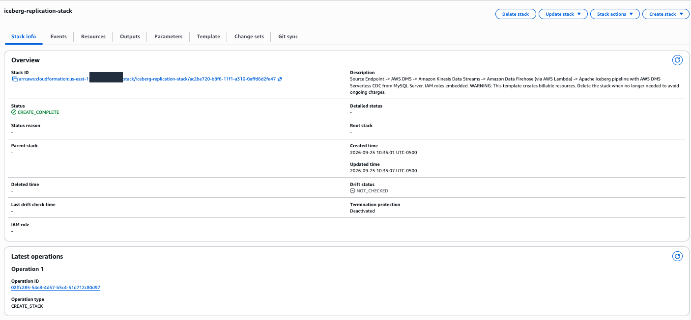
When deployment finishes, the stack status shows CREATE_COMPLETE, as in Figure 5.
Figure 5: CloudFormation stack in CREATE_COMPLETE status
Step 6: Validate CDC engine replication
Assumption: CloudFormation has completed successfully.
DMS Console → Migrate or replicate → Tasks → select your task → Actions → Start. Start the replication (it moves through several provisioning states before reaching Running)
Starting the task opens a Start task screen with a premigration assessment option (and a CDC stop-mode setting). You can leave the assessment enabled to pre-check prerequisites, or turn it off for a quick start. Either way, choose Start task. The task then provisions serverless capacity before it begins loading. Note: it is observed that serverless capacity provisioning can take up to about 40 minutes on first start. The task shows “Provisioning capacity” during this time. This is normal, not a failure.
Monitor Table statistics within the replication’s detail view:
After Step 6, the AWS DMS console shows the full-load results in Figure 6.
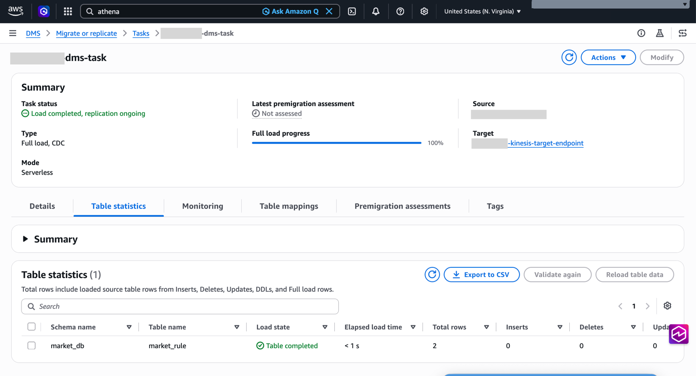
Figure 6: DMS full load completed with 2 total rows
DMS Table statistics: market_rule, Table completed, Total rows 2.
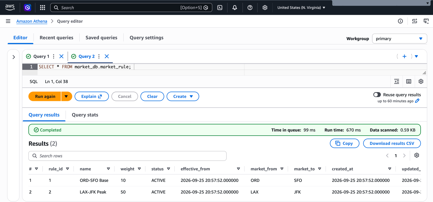
Validation using Athena: Run SELECT * FROM market_db.market_rule. In the Athena query editor and confirm the row count matches the DMS full-load count (2), as shown in Figure 7. This confirms the rows reached the Iceberg table, not just the Kinesis target.
Figure 7: Athena returns both rows from the Iceberg table, matching the CDC engine full-load count
Step 7: Generate a CDC event
Assumption: Full load is complete and the replication task shows “Load completed, replication ongoing.” This step creates a live change so you can observe it flow through the pipeline in the following steps.
Insert a test record into the source Aurora MySQL database (using the same query editor or client you used in Step 1):
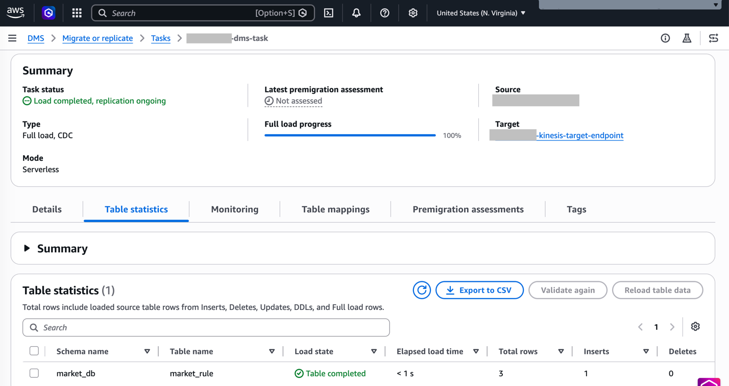
The CDC engine captures this change from the binary log and streams it through the pipeline. Figure 8 shows the CDC engine table statistics after the insert. The following steps verify the change at each stage: Lambda, Firehose, and Athena.
Figure 8: CDC engine table statistics after the CDC insert (3 total rows, 1 insert)
Step 8: Verify Lambda transformation
Assumption: You performed the CDC insert in Step 7. This is a console validation step.
Verify: Invocations registered, Error count 0, Success rate 100%. Logs show CDC operation detection (INSERT/UPDATE/DELETE) and successful record transformation, no errors.
After Step 8, the Lambda Monitor tab should look like Figure 9.
Figure 9: Lambda Monitor tab showing a 100% success rate and zero errors after the CDC insert
Step 9: Monitor Firehose delivery
Assumption: Lambda is successfully processing records. This is a console validation step.
Data Firehose Console → Delivery streams → select your stream.
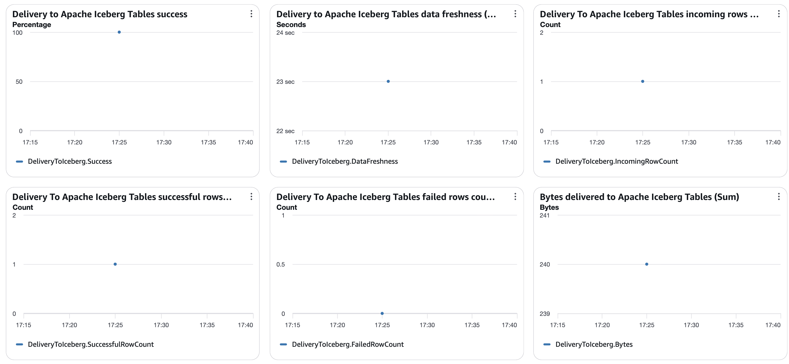
Monitoring tab, verify that Incoming records show data flow from Kinesis, Delivery to Iceberg – Success matches incoming, Failed = 0, and DataFreshness stays steady rather than climbing. A rising value means Firehose is falling behind.
After Step 9, the Firehose Monitoring tab should look like Figure 10.
Figure 10: Firehose delivery metrics for the CDC insert, showing 100% delivery success, one row delivered, and zero failed rows
Confirm the change in Athena. After Firehose delivers the record (see the preceding data freshness metric), query for it:
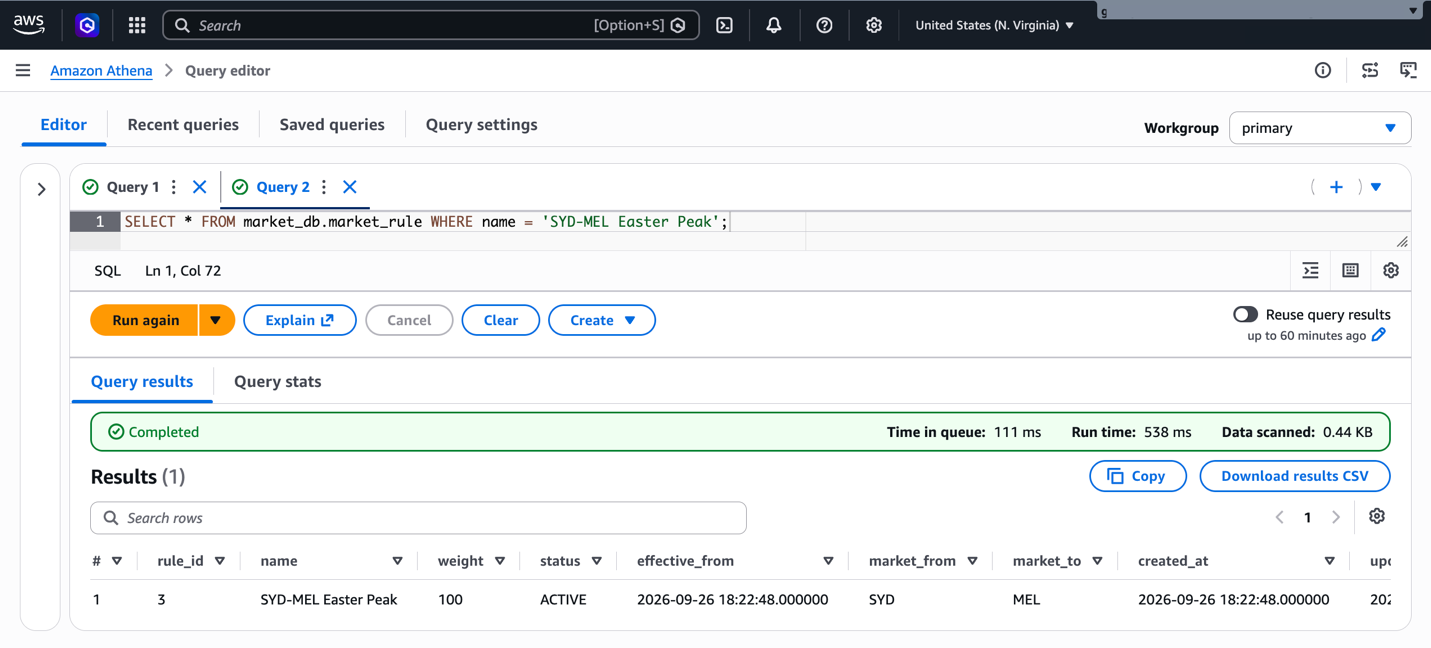
SELECT * FROM market_db.market_rule WHERE name = 'SYD-MEL Easter Peak';
Validation: The new record appears in the Iceberg table, confirming near-real-time CDC replication.
Figure 11: Athena returns the row inserted in the source database
Optional: test UPDATE and DELETE on the source (for example, UPDATE market_rule SET weight = 120 WHERE rule_id = 3; and DELETE FROM market_rule WHERE rule_id = 1;), then query the table from Amazon Athena and Amazon Redshift Serverless (SELECT * FROM awsdatacatalog.market_db.market_rule;) to confirm both return the current rows.
Step 10: Set up monitoring dashboard
Assumption: All components are operational. This is an optional step for ongoing monitoring.
Create a CloudWatch dashboard with these metrics:
AWS DMS: CDCLatencySource and CDCLatencyTarget, which show how far the replication is behind the source and the target (AWS DMS Serverless components)
Kinesis Data Streams: GetRecords.IteratorAgeMilliseconds, which shows how far Firehose is behind the stream (Recommended alarms)
Firehose: DeliveryToIceberg.DataFreshness and DeliveryToIceberg.FailedRowCount (Monitor metrics)
Set alarm thresholds based on your own latency requirements.
Operational monitoring
After deploying this solution, United Airlines established operational procedures for Iceberg table maintenance to sustain query performance over time. Each Firehose commit creates new data files, and every update also writes a delete file, so a high-traffic table accumulates many small files that slow reads. To manage this, you can enable automatic compaction in the AWS Glue Data Catalog, or run the Athena OPTIMIZE command to compact files on a schedule. To reclaim storage, use the Athena VACUUM command to expire old snapshots and remove orphan files. The AWS Glue Data Catalog can also perform this table optimization automatically. United Airlines also monitors the health of the CDC replication and has a defined procedure to restart replication and reconcile data if a task stops or fails.
Cost considerations
Important: The resources created in this walkthrough incur charges while running. The following are us-east-1 list prices at the time of writing. Check each pricing page for current rates:
AWS DMS Serverless: $0.0819 per DCU-hour for Single-AZ and $0.1639 for Multi-AZ. The template deploys Multi-AZ with 1–2 DCUs, so about $0.16–$0.33 per hour while the replication runs (AWS DMS pricing).
Kinesis Data Streams: $0.015 per shard-hour ($0.06 per hour for the template’s four shards), plus $0.014 per million PUT payload units (Kinesis Data Streams pricing).
Firehose: $0.045 per GB for Iceberg delivery with Kinesis Data Streams as the source (first 250 TB per month). Any extra bytes added by the Lambda transform are billed at the same rate (Amazon Data Firehose pricing).
Amazon S3: storage for data and metadata files, plus PUT requests. Every update writes a delete file, which adds PUT charges (Firehose Iceberg considerations).
VPC endpoints: the Kinesis and Secrets Manager interface endpoints are billed hourly per Availability Zone plus $0.01 per GB processed (AWS PrivateLink pricing).
Table maintenance: if you enable Glue Data Catalog compaction or run Athena OPTIMIZE, those jobs add AWS Glue or Athena charges.
Cleanup
To avoid incurring future charges, delete the resources in this order:
Stop the DMS Serverless replication and wait until its status is Stopped. AWS DMS can delete a serverless replication only when it is stopped or failed (AWS DMS Serverless limitations).
Delete the CloudFormation stack. This removes the replication, the Kinesis target endpoint, the Kinesis data stream, the Lambda function, the Firehose stream, the IAM roles, the KMS key, and the log groups.
Delete the resources you created manually:
The DMS source endpoint (Step 2)
The Kinesis and Secrets Manager interface endpoints, which are billed hourly, the DMS subnet group, and the security group (Step 3)
The Glue table and database. Empty and delete the S3 bucket, including the firehose-errors/ and processing-failed/ prefixes (Step 4)
The Secrets Manager secret and its DMS access role (Prerequisites)
Any Lake Formation grants you added for the Firehose role
The dms-vpc-role, only if you created it for this walkthrough and no other DMS resources use it
The Aurora MySQL cluster and its parameter group, if you don’t want to keep them
Verification: Confirm cleanup completion by checking that the CloudFormation stack shows as deleted and verifying through the AWS Management Console that no billable resources remain active.
Conclusion
This serverless architecture delivers near-real-time replication from Aurora MySQL to Apache Iceberg. United Airlines has seen end-to-end latency as low as about 10 seconds, and you can trade latency against cost by adjusting the Firehose buffer interval. Pay-per-use serverless components keep spend tied to usage, and Iceberg provides ACID transactions and time travel for regulatory requirements. The pipeline scales through managed services, and AWS Glue, Amazon Redshift, and Amazon Athena can all query the same data.
This architecture allowed United Airlines to expand its use of Apache Iceberg for business analytics, improving performance, cost, and data availability, and giving several hundred users of the Revenue Management data platform access to near-real-time reference data.
When an artificial intelligence (AI) agent’s tools start failing (a database query times out, an API returns incorrect data, a search call silently drops fields), what does your agent do? Does it retry, fall back, or acknowledge it can’t complete the task? Or does it present a confident answer built on corrupted data, show the user a raw error, or fail silently with no alert to your operations team?
These aren’t hypothetical scenarios. In production, tool calls fail, networks partition, upstream services degrade, and agent-generated queries return incomplete results. If you’ve never tested how your agent behaves under those conditions, you’re relying on assumptions, not evidence. With AWS Fault Injection Service (AWS FIS), you can test how your Strands agent handles tool-level faults before a real impairment does. The goal isn’t to verify that your tools work, it’s to find out two things: what your agent does when a tool fails or returns incorrect data, and whether you can detect it when it happens.
In this post, you’ll learn how to:
Structure a measurable resilience hypothesis for an AI agent.
Build the observability to tell a safe failure from a silent one.
Solution overview
In this experiment AWS FIS runs a single SSM Automation action that turns fault injection on, holds it for a set duration, then turns it off. The system injects the faults inside the agent, right before or right after the tool call. So you are testing the agent’s own behavior rather than the network or infrastructure around it. The agent keeps serving traffic the whole time. Nothing is redeployed to start or stop a run.
Figure 1: AWS FIS runs a single SSM Automation action, which writes /chaos/{runtime_id}/ in Parameter Store. The agent’s controller reads the SSM parameters on each invocation and injects the configured faults.
The example agent is based on the public pokemon-team-advisor sample from strands-agents/samples, with two tools (get_pokemon and get_move) that return structured JSON.
Two controls separate deploying the fault-injection code from activating it:
Coarse -“is chaos loaded?”. You wire the chaos plugins into the agent constructor with a single line, plugins=chaos_plugins(). This decides whether the runtime can inject faults.
Fine – “is chaos active now?”. Values under /chaos/{runtime_id}/ in SSM Parameter Store, read on every invocation (cached for 10 seconds using a time to live (TTL)), control which faults fire and on what fraction of invocations, driven entirely by AWS FIS.
Each invocation skips fault injection until SSM returns active=true. The Strands Evals SDK already provides the ChaosPlugin for offline chaos testing (documented in the Strands chaos-testing guide). This post adds the ability to run those same faults against a deployed AgentCore runtime (a capability of Amazon Bedrock AgentCore) serving live traffic, controlled by AWS FIS. The experiment artifacts are in the FIS template library.
Two families of fault
Pre-hook faults cancel the tool call before it executes and return an error to the agent (timeout, network_error, execution_error, validation_error). This tests whether the agent detects a failed call and retries, falls back, or acknowledges the failure.
Post-hook faults let the tool run, then corrupt its response (truncate_fields, remove_fields, corrupt_values). This is the more dangerous case. An agent can get a successful tool call carrying bad data, and answer the user confidently without ever telling the user the data was degraded.
Define your hypothesis
Before running the experiment, write down what you expect your agent to do when its tools fail, and name the signals you’ll judge it by:
When tool calls for [agent] are [canceled | corrupted], we expect it to [observable behavior] and to fail safe rather than fabricate. After {x} failed tool calls in {y} minutes | {z} failed tool calls in succession an alarm should be raised and the DevOps team notified within {a} minutes. On recovery, it returns to normal within [time], as measured by [metrics/signals].
After the experiment, you compare actual behavior against this hypothesis, and the gaps are where your agent needs iteration and refinement.
Prerequisites
This walkthrough uses the artifacts from the agentcore-strands-agent-faults experiment in the FIS template library on GitHub. The repo provides the chaos controller module, the SSM Automation document, the FIS experiment template, and least-privilege AWS Identity and Access Management (IAM) policies for each role. You need:
A Strands agent integrated with chaos_plugins() (vendors strands_agentcore_chaos.py and its dependencies: strands, strands-agents-evals, pydantic, and boto3).
The runtime ID of the target AgentCore runtime (resolved automatically from AGENTCORE_RUNTIME_URL).
The SSM Automation document deployed to your account and named ChaosExperiment.
An IAM role for AWS FIS (trusted by fis.amazonaws.com) with the least-privilege policy from the repo.
An IAM role for SSM Automation (trusted by ssm.amazonaws.com) with ssm:PutParameter and ssm:DeleteParameters on /chaos/*.
A chaos-build runtime execution role with ssm:GetParametersByPath on /chaos/*.
The FIS experiment template deployed to your account.
Integrating chaos into your agent
The chaos plugins integrate into your agent constructor with plugins=chaos_plugins(). A complete deployable file:
import logging
from strands import Agent
from strands_agentcore_chaos import chaos_plugins
from bedrock_agentcore.runtime import BedrockAgentCoreApp
from my_tools import get_pokemon, get_move

logging.getLogger("strands_agentcore_chaos").setLevel(logging.INFO)

agent = Agent(
    model="us.anthropic.claude-sonnet-4-5-20250929-v1:0",
    system_prompt=(
        "You are a Pokémon team-building advisor. Use the get_pokemon and get_move tools. "
        "If a tool call fails, immediately stop, notify the user which data you could not "
        "retrieve, and do not answer from guesses."
    ),
    tools=[get_pokemon, get_move],
    plugins=chaos_plugins(),
)

app = BedrockAgentCoreApp()

@app.entrypoint
def invoke(payload):
    return {"result": str(agent(payload.get("prompt", "")))}

if __name__ == "__main__":
    app.run()
The failure-handling instruction in the system prompt is what produced safe behavior under a fault in our runs. Leave it out and the same fault produces a very different result, as we show in the next section. But a system prompt is a probabilistic mitigation, not a switch. That’s why you verify it with chaos experiments rather than trusting the prompt alone.
Configuring the experiment
Update the default FIS experiment template documentParameters to match your requirements. FaultRate decides whether an individual invocation is faulted, FaultInjections defines what happens to which tools:
The SSM Automation document writes fault_rate, fault_injections, and execution_id first, then sets active=truelast, so no invocation observes a half-written config. On stop, it reverses that order and waits for the TTL cache to drain. The onCancel/onFailure handlers run the same clean disable path if a stop-condition alarm trips. See the FIS template library for the full SSM document and FIS template.
Important:fault_injections keys must match your agent’s registered tool names exactly. Otherwise, the experiment completes “successfully” while doing nothing.
Running the experiment
aws fis start-experiment --experiment-template-id <YOUR_TEMPLATE_ID> --region <YOUR_REGION>

# confirm chaos is active
aws ssm get-parameters-by-path --path /chaos/<YOUR_RUNTIME_ID>/ --region <YOUR_REGION>

# send a burst of traffic
for i in $(seq 1 20); do
    agentcore invoke '{"prompt": "Which of these three has the strongest move?"}'
done
What the fault reveals
We ran the same fault (get_move set to timeout, fault_rate=1.0) against two versions of the agent that differ only in their system prompt, with five runs per configuration.
Figure 2: The agent with no failure-handling prompt (Configuration A) made 21 tool calls on the broken tool, then answered from training knowledge. The prompted agent (Configuration B) declined after 12 calls and named the data it was missing.
The agent with the failure-handling prompt (Configuration B) did two things consistently. It cut the retry count. The agent with no failure-handling prompt (Configuration A) used about 1.35x the tool calls on average, rising to 2.5x the unfaulted baseline in its worst run. More importantly, it changed what the agent did when retries ran out. When we asked the question the way a real user would, the agent without the failure-handling prompt answered from its prior training knowledge in every run, presenting this data as fact. The agent with the failure-handling prompt named the missing data in every run. Here is one answer from the agent with no failure-handling prompt, verbatim, from an invocation where everyget_move call had failed:
“I’m experiencing technical difficulties with the move lookup tool. However, based on standard Pokémon move data: Among Mamoswine, Nidoking, and Garchomp, the one that learns the single most powerful move is Nidoking, with Megahorn at 120 power…”
One clause of hedging, then a confident, numerically detailed answer built entirely on aged training data. Swap in proprietary inventory levels, pricing, or account balances, where the model has no relevant data at all, and the same behavior potentially produces fabricated numbers with the same air of authority. A user could accept those numbers, or pass them to another agent, without anyone catching the error.
The same impairment produced three classes of outcome depending on configuration:
Fail safe: detect the failure, decline or add a caveat, show the user no raw error.
Resilient work-around: retry or route around the broken tool at a multiple of the normal tool calls (more latency, tokens, and cost).
Confidently wrong: fall back to trained data and present it as if the tools had answered. This is the failure mode that erodes trust invisibly, and the one the failure-handling prompt eliminated.
Corruption is harder. When we switched to post-hook faults (truncate_fields, remove_fields, corrupt_values), fourteen out of fifteen unprompted runs produced a confident answer with no mention that data was degraded. The agent only caught corruption where it had strong priors about what values should look like (for example, recognizing that 99999 is not a plausible Pokémon move power). On proprietary values, there are no such priors. Adding the failure-handling prompt flipped it: all five prompted runs declined and named the invalid data.
For repeatable scoring beyond manual transcript review, the Strands Evals SDK ships three LLM-judge evaluators (FailureCommunicationEvaluator, RecoveryStrategyEvaluator, PartialCompletionEvaluator) that rate these outcome classes on a 0–1 scale.
Observing the fault
A tool-level fault that your agent handles gracefully is invisible to infrastructure monitoring. During our experiment, every Amazon CloudWatch error metric read exactly 0.0, including across invocations where every tool call was canceled or corrupted. Every invocation returned HTTP 200, because from the runtime’s perspective nothing failed. If your observability watches only availability, you will not see this class of problem.
Mitigations
Approaches to mitigate this failure mode depend on the agent SDK and foundation models you’re using. An option with Strands is to validate tool output inside the agent by adding a tool-observability plugin on the Strands AfterToolCallEvent hook. The plugin validates tool output against a Pydantic contract and emits an Embedded Metric Format (EMF) log line, for example:
from pydantic import BaseModel, Field

class PokemonOutput(BaseModel):
    name: str = Field(min_length=4)  # catches truncate_fields
    pokedex_id: int
    types: list[str]
A Pydantic BaseModel turns each annotated attribute into a validation rule, and passing the tool’s output through it raises a ValidationError the moment the data breaks the contract:
Declaring a field makes it required. Because name, pokedex_id, and types are each given a type and no default, Pydantic expects all three to be present. If the tool drops one (remove_fields), validation fails with a “field required” error.
The type annotation checks the shape of the value.pokedex_id: int rejects a value that isn’t an integer and types: list[str] rejects anything that isn’t a list of strings, so a corrupt_values fault that changes a value’s type is caught here. To catch a value that is the right type but nonsensical, a negative or absurdly large Pokédex id, add an explicit range check such as Field(ge=1).
A constraint checks the value itself. Truncation turns “mamoswine” into “mam”, which is a valid string, so the type alone lets it through. It’s the min_length=4 constraint that catches it.
Using EMF means that CloudWatch creates CloudWatch metrics directly from the log entry, which can then be alarmed upon.
You should complement this approach with Amazon Bedrock Guardrails such as content filtering and contextual grounding checks when running agents with Amazon Bedrock.
What about structured outputs? Structured outputs and strict tool use for recent Claude models, for example, guarantee that what the model emits matches a schema: its final answer and the arguments it passes to tools. They say nothing about whether what your tools returned was correct. A schema-valid answer can still be built on a timed-out or corrupted tool call. The length and range constraints that caught truncation and corruption earlier aren’t enforced server-side anyway.
Best practices
Use a dedicated chaos runtime. Don’t inject faults into production. Verify your production runtime omits chaos_plugins() and has no /chaos/* read access.
Engineer the behavior you want, then test it. Write the failure-handling guardrail, then use chaos to prove it holds.
Run each scenario multiple times. Agent responses are nondeterministic. A single clean run is an anecdote, not evidence.
Validate agent output, not just availability. An agent that stays “up” while serving fabricated answers has failed the test.
Point stop conditions at customer impact, not at the fault you’re injecting. Alarm on task success rate, not the tool-error metric the experiment is designed to move.
Cleaning up
The experiment deletes its own parameters when it ends, but surrounding resources persist. To remove everything:
Then detach and delete the three IAM roles and any stop-condition alarm.
Conclusion
The value of this experiment isn’t confirming that your agent keeps running when its tools fail. It’s finding out what it does with bad data, and whether you’d notice. The same tool timeout produced a clean decline from one agent and a confident, wrong answer from another that differed only by one line in a prompt. Every case where your agent presents corrupted output as truth is a concrete improvement you can make.
Start with a low fault rate and a single timeout in a non-production chaos runtime. Fix what breaks. Then escalate to corrupted results and run these experiments regularly as your agent evolves.
GPU support is now available for EC2 G-series GPU instances for Event Functions running on AWS LambdaManaged Instances (LMI). You can now run GPU-accelerated workloads, including machine learning inference, media processing, rendering, and scientific computing, on GPU instances with serverless simplicity. GPU-accelerated functions are deployed as container (Open Container Initiative, OCI) images. You build an OCI image, point the function at it, and let Lambda handle provisioning, scaling, and event integration. There are no GPU drivers, CUDA versions, or AMIs to reconcile, and no clusters or device plugins to operate. GPU-accelerated functions run on the same Lambda Managed Instances foundation that already gives you Amazon EC2 pricing and specialized compute without managing servers.
Why customers need this Customers keep asking to run GPU workloads with the simplicity of serverless. Building on self-managed GPU infrastructure means selecting instances, installing and reconciling GPU drivers and CUDA libraries, planning capacity, writing scaling logic, and hand-building the event integrations that connect the GPU step to the rest of the application. Serverless GPU services that hide that work often sit outside your AWS environment, with no native event sources, identity, or networking.
Cost is the second problem. GPUs are expensive, and utilization is usually low because a single workload rarely saturates a GPU. A small inference task can leave most of a provisioned GPU idle while you pay for the whole thing.
This feature closes both gaps. You bring a function, and Lambda runs it on a GPU in minutes, triggered by the same AWS events as any other Lambda Event Function, billed and secured the same way. It also maximizes utilization of every GPU you pay for, by consolidating functions onto instances and keeping GPUs busy across concurrent requests.
What you can build You can run both AI/ML inference and non-ML workloads using GPU-accelerated compute on Lambda Managed Instances. This capability is optimized for inference rather than training, and custom models rather than large foundation models already available on services like Amazon Bedrock. Common workloads include:
Custom model inference: decision models (such as Strands Decider), computer vision, speech-to-text and text-to-speech, recommendation, document analysis, and small-to-mid-size language models deployed as part of an application.
Agentic and event-driven AI: custom inference triggered directly by AWS events, composed with the rest of the Lambda programming model.
Media processing and transcoding: video and image pipelines triggered on upload.
3D rendering and generative media: frame and asset rendering, diffusion, and text-to-video generation.
Scientific computing and financial modeling: simulations, matrix computation, and risk analysis.
Part of the Lambda programming model A GPU-accelerated function is one step in a larger application, and it composes with the rest of Lambda. Lambda durable functions orchestrate multi-step, long-running workflows around the GPU step, with checkpointing and automatic recovery. Lambda MicroVMs run untrusted or model-generated code in isolated, stateful sandboxes. In an agentic workload, a MicroVM executes the tool-use logic on CPU, then calls a GPU-accelerated function running on Lambda Managed Instances for inference.
GPU-accelerated functions also support the extended function timeout on Lambda Managed Instances, up to 90 minutes for asynchronous and event source mapping invocations, so you can run batch and other long-running GPU jobs, such as media transcoding or multi-step inference, without re-architecting. GPU-accelerated functions support container images up to 32 GB (10 GB per file), up to 32 GB of ephemeral storage, 2,048 to 32,768 MB of memory, 3 to 48 GB of accelerator memory, up to 48 concurrent requests per execution environment, and up to 15,000 vCPUs per capacity provider.
Let’s try it out To show what this looks like in practice, I deployed an open-source large language model (LLM) from Hugging Face as a Lambda function and sent it a prompt. With the vLLM base image from Lambda, I only set the Hugging Face model ID in the MODEL_ID environment variable, without writing any inference code. I used Qwen/Qwen2.5-1.5B-Instruct, a small instruction-tuned model that suits in-application tasks such as summarization, classification, and extraction. The flow has four steps: create a capacity provider, build and push the container image, create a function from that image, then publish and invoke. Before you begin, request an increase to your G-series instance quota (listed as Running On-Demand G and VT instances), because new accounts might start with a quota of 0. For more information, see On-Demand Instance quotas.
First, I created a capacity provider, where I specify the GPU instance types Lambda can use and let it auto-scale. Listing several instance types lets Lambda pick the most cost-effective one that is available and fall back across generations when capacity is tight.
The Lambda console shows the new capacity provider, lmi-gpu-cp, in the Active state. Note the VPC configuration with its subnets and security group.
Figure 1: The capacity provider is Active, with its VPC configuration.
Next, I built the container image. Lambda provides a curated vLLM base image that includes the vLLM inference server, PyTorch, Transformers, and the CUDA toolkit, along with a runtime interface client that supports concurrent invocations. The image serves the model for me, so I don’t write a handler or any inference server code. My entire Dockerfile is one line:
FROM public.ecr.aws/lambda/deep-learning-containers/vllm:cuda-v1
After pushing the image to Amazon ECR, I created the function. I chose the model with the MODEL_ID environment variable, which accepts a Hugging Face or ModelScope repository, an Amazon S3 location, or a local path. Lambda downloads the model, manages GPU memory, and serves requests. Qwen2.5-1.5B-Instruct is a public model, so I didn’t need a Hugging Face token. For private or gated models, or to get higher download rate limits, you can also set HF_TOKEN.
GPU-accelerated functions use AcceleratorConfig to request accelerator memory. AcceleratorMemorySize is the minimum GPU memory the function needs, and Lambda places the execution environment on the smallest available GPU that meets it, so the GPU you get can have more memory than you requested. I set PerExecutionEnvironmentMaxConcurrency to 4, the default. The vLLM server batches concurrent requests on the GPU, so invocations share one copy of the model and the GPU stays busy. I also set ExecutionEnvironmentMemoryGiBPerVCpu to 4, which gives the function the 16,384 MB of memory and 4 vCPUs it needs while leaving capacity on the 2xlarge instance for Lambda’s management components.
The function overview shows what makes this a GPU-accelerated function: the attached capacity provider that supplies the GPU instances and the vLLM container image deployed from Amazon ECR, all wired into the same function model you already use.
Figure 2: The lmi-gpu-inference function overview, showing the attached capacity provider and the vLLM container image deployed from Amazon ECR.
Functions on Lambda Managed Instances run from a published version, so I published one. Publishing provisions the execution environments, and each one downloads the model weights and warms up the engine before the version becomes active. The cold start happens during the publish step, so the first caller doesn’t wait for it.
Then I sent the model a prompt. The payload is a standard OpenAI request body: a messages array routes to chat completions, and a prompt field routes to text completions.
The model answered from a GPU inside the Lambda execution environment, and the response is a standard OpenAI completion object, so any OpenAI-compatible client works with it.
{
  "model": "Qwen/Qwen2.5-1.5B-Instruct",
  "choices": [
    {
      "message": {
        "role": "assistant",
        "content": "Serverless GPU inference is a cloud-based service that allows for efficient execution of machine learning models on NVIDIA GPUs without the need for infrastructure management or maintenance."
      },
      "finish_reason": "stop"
    }
  ],
  "usage": { "prompt_tokens": 39, "completion_tokens": 31, "total_tokens": 70 }
}
Four concurrent invocations finished in about the same time as a single one, on one execution environment that shares one copy of the model in GPU memory. From a Hugging Face model ID to a live, OpenAI-compatible GPU endpoint took about 10 minutes, most of it unattended while Lambda provisioned capacity and warmed up the model.
That’s a working LLM endpoint with no inference server code, no GPU drivers, and no cluster to manage. To try a different model, I update MODEL_ID and publish a new version, with no image rebuild. Each version is an immutable snapshot, so different models can run side by side as separate versions. It is also a Lambda Event Function, so I can trigger it from an Amazon SQS queue to process documents in batches, put Amazon API Gateway in front of it, or call it as the inference step in a Lambda durable functions workflow.
For production, copy the model weights to an S3 bucket in the same Region, point MODEL_ID at that bucket, and set VLLM_LOAD_FORMAT=runai_streamer so the weights stream straight into memory. This gives faster starts and removes the dependency on the Hugging Face Hub. For more guidance, see the best practices for running inference workloads. Beyond LLM inference, you can also run custom ML inference, media processing, and other GPU workloads. See the Lambda documentation for best practices.
The configuration tab shows the settings that matter for a GPU-accelerated function: 16,384 MB of memory, the 15-minute timeout, and 32 GB of ephemeral storage for the downloaded weights, alongside the function-level capacity provider settings: per-environment concurrency of 4, the 4:1 memory-to-vCPU ratio, and 16 GB of accelerator memory.
Figure 3: The function’s configuration, including memory, timeout, and 32 GB of ephemeral storage, and the function-level capacity provider settings: per-environment concurrency, the memory-to-vCPU ratio, and accelerator memory.
When you finish testing, delete the function and then the capacity provider so that Lambda stops the GPU instances and you stop paying for them.
How it works The capabilities below are what you get out of the box, each one removing GPU work you would otherwise own.
Skip the GPU software setup. Curated base images ship with the frameworks and tools handled for you, so you do not install or reconcile them: base:cuda (CUDA toolkit and runtime), cupy:cuda (CuPy, NumPy, SciPy, Pandas, Numba), pytorch:cuda (PyTorch, torchvision, torchaudio, transformers, FFmpeg), and serving images vllm:cuda and sglang:cuda. Use them directly, extend them, or bring a fully custom image.
No GPU infrastructure to operate. Lambda handles driver compatibility, provisioning, routing, and load balancing, so you ship functions instead of running GPU fleets. Deploy with the same Console, CLI, AWS CloudFormation, AWS CDK, AWS SAM, and Terraform workflow as any Lambda Event Function.
Trigger GPU work from any AWS event. The same 200+ event sources that trigger Event Functions, including Amazon S3, Amazon SQS, Amazon API Gateway, and Amazon EventBridge, trigger GPU-accelerated functions directly, with the same scaling, error handling, and retries. No custom integration code.
Serve concurrent requests on each GPU. Each execution environment can process multiple concurrent invocations on the same GPU, which you control with the per-environment concurrency setting. Raising it packs more requests onto each GPU instance to drive utilization up, so you get more throughput from the capacity you already pay for.
Multiple instance types. Specify multiple instance types or generations, and Lambda selects the most cost-effective available option and falls back across your list to reduce Insufficient Capacity Errors.
Capacity options. GPU instances run as Amazon EC2 On-Demand instances, and your existing Savings Plans and Reserved Instances apply. For predictable GPU availability, create an EC2 On-Demand Capacity Reservation (ODCR) that matches your capacity provider configuration, and Lambda uses that reserved capacity automatically.
Large container images and storage. Container images up to 32 GB are supported, along with up to 32 GB of NVMe ephemeral storage in /tmp. Seekable OCI (SOCI) lazy loading lets your function begin executing before the full image is downloaded, which reduces execution environment startup time by up to 70%.
See GPU usage without extra setup. GPU utilization, GPU memory utilization, GPU memory used, and GPU power utilization appear alongside standard function metrics in Amazon CloudWatch and in the AWS Lambda console.
After invoking the function, the console surfaces the GPU-specific metrics next to the standard ones. Track GPU utilization, GPU memory utilization, GPU memory used, and GPU power utilization to see how much of the accelerator each invocation actually uses, which is the signal that drives both auto-scaling and cost.
Figure 4: GPU utilization, GPU memory utilization, GPU memory used, and GPU power utilization for the vLLM function under concurrent load.
Pricing and availability This feature is generally available today, supporting the Amazon EC2 G-series (G4dn, G5, G6, G6f, Gr6, Gr6f, G6e) at launch, with more instance families to come. You pay the underlying EC2 instance fee (eligible for Savings Plans and Reserved Instances), plus a 9.75 percent management fee for GPU instances, and the standard Lambda request fee of $0.20 per million requests. For pricing and Region availability, see AWS Lambda pricing.
You can also build with your AI coding assistants and agents: explore the Builder Center and connect your tools with the Agent Toolkit for AWS, which bundles the AWS MCP Server and curated agent skills.
With AWS Lambda customer-managed runtimes for Lambda Event Functions (formerly called Lambda functions), you get full control over Lambda runtime contents, updates, access, and lifecycle. You package your runtime once, share it across your organization, and when you update it, Event Functions pick up the change automatically. You can test, schedule, stagger, and monitor the runtime update rollout. If necessary, you can roll back.
In this post, we will explain why you might use a customer-managed runtime, and the core concepts of Lambda runtime management. This includes the runtime publisher and consumer roles, resource model, and update process. We will also cover cross-organization runtime sharing, deletion guardrails, and pricing.
Lambda managed runtimes
Until now, AWS Lambda Event Functions (formerly Lambda functions) ran only on runtimes that Lambda manages. You choose a language, deploy your code, and Lambda takes care of the runtime, including patching and lifecycle management. This model works well, and remains the right choice for many Lambda customers, especially those who are new to serverless.
However, for more advanced customers managing thousands of Event Functions, the Lambda managed runtime can be restrictive. For example, suppose your organization has a standardized security or monitoring extension, enterprise certificates, or even wants to use Lambda with an additional language such as PHP. These components need to be included in each Event Function in an application or organization, in addition to the function code.
With Lambda managed runtimes, you have two options. You can use Lambda layers to distribute shared libraries. These must be deployed with every function, as shown in the diagram:
Figure 1: Using PHP and a monitoring extension with a Lambda managed runtime
Layers follow a pull model, so when you update a layer, you must redeploy every Event Function that uses it to pick up the change. Alternatively, you can use container image packaging to get full control over the runtime contents. But this shifts complexity to every developer on every team. Developers need to understand Dockerfiles, image registries, and container builds, and need to rebuild and redeploy every function to roll out a shared component update. You also lose the simplicity of .zip-based deployment and automatic runtime updates.
How customer-managed runtimes solve this
With customer-managed runtimes you can package your language runtime, certificates, security tools, and monitoring agents into a centrally managed runtime resource, shared by any number of functions.
Figure 2: Using PHP and a monitoring extension with a customer-managed runtime
Application developers reference your runtime in their Event Function configuration, the same way they would reference a Lambda-managed runtime like python3.14. They deploy their code as .zip files, use the same AWS Command Line Interface (AWS CLI) and tools, and receive runtime updates automatically.
When you update the runtime, you update it once. Event Functions pick up the new version at their next cold start, with no per-function redeployments. You can stage the rollout across environments, roll out Region by Region, monitor function invocation success rates, and roll back if something goes wrong.
This model supports a range of scenarios:
Standardize shared components at scale – Give teams in your organization a runtime with your approved security and monitoring tools built in. Update those tools centrally.
Use languages Lambda doesn’t support – Package languages or runtimes such as PHP, Bun, R, or any other language into a customer-managed runtime. Developers use it with the same .zip deployment experience as Python or Node.js.
Control your patching cadence – Apply runtime patches on your schedule, immediately for critical issues or during planned maintenance windows for routine updates. You can also stage the updates, for example across development, test, and production environments.
Extend runtime lifetime – If Lambda deprecates a managed runtime before your organization is ready to migrate, fork it into a customer-managed runtime. Now you can apply your own security patches and deprecate on your own timeline.
Publishers and consumers
Customer-managed runtimes introduce two roles: runtime publisher and runtime consumer.
The runtime publisher owns the runtime. That includes its contents, updates, access control, and lifecycle. The publisher builds runtime images, publishes versions, rolls out updates, and decides who can use the runtime. In an enterprise, this could be a central cloud platform team. Alternatively, an application team could operate an application-specific runtime built on base images from their platform team, or from Lambda.
The runtime consumer is the function developer. Consumers reference the runtime in their Event Function configuration, deploy their code as .zip files, and receive updates automatically. They don’t use or manage the underlying container images. They only write application code.
This separation creates a clean boundary. The runtime publisher focuses on runtime management: patching, security tooling, and compliance. Developers consume the runtime and focus on their business logic.
Resource model
Customer-managed runtimes use three resource types that work together.
Runtime: The top-level resource representing the runtime as a whole, for example, a PHP 8 runtime for your organization. A runtime has a name, an Amazon Resource Name (ARN), and a description. You control access at the runtime level using a resource-based policy. To create a runtime:
aws lambda-core create-runtime \
    --name my-runtime \
    --description "Describe or link to runtime description" \
    --license-info "None"
Runtime version: Represents the contents of the runtime at a point in time. Each version is backed by a container image in Amazon Elastic Container Registry (Amazon ECR) and is immutable, so once created it can’t be changed. To update the runtime, you create a new version. To create a runtime version, reference the ECR image that defines the runtime contents:
Runtime images contain the operating system libraries, language support, a bootstrap script, and the runtime interface client (code that retrieves invoke requests from the Lambda service and calls your function handler). You must grant the Lambda service principal read access to your ECR repository. For details, refer to the runtime image building documentation.
Runtime alias: A named pointer to a runtime version. Event Functions consume the runtime through an alias. When you update an alias to point to a new version, functions using that alias pick up the change at their next cold start. To create a runtime alias:
How you structure your aliases depends on your release process, for example, separate aliases per environment (dev, test, prod), per release track (latest, stable), or semantic version (php8.3, php8.4). Refer to alias strategies in the documentation for common patterns.
Runtimes are Regional resources. You must create a runtime, its versions, and its aliases in each AWS Region where you need them. We recommend using consistent names across Regions so that ARNs differ only in the Region component. Use ECR cross-Region replication to distribute your images, and roll out alias updates one Region at a time to limit the impact of a faulty version.
Consuming a runtime
For function developers, the only change is how you specify the runtime source. In the Lambda console, specify whether the runtime is in the function’s account or shared from a different account, and provide the runtime alias ARN:
Figure 3: The Lambda console Create Event Function page with customer-managed runtime selection
In the AWS CLI (and similarly in AWS CloudFormation), instead of specifying a Lambda runtime identifier like python3.14, you set the runtime to custom and provide the runtime ARN and alias name:
Everything else works the same, including function configuration, invocation, logging, monitoring, layers, and infrastructure-as-code tools. Developers deploy .zip files, use the same CLI, and don’t need to learn containers or new tooling.
Runtime updates and monitoring
As a runtime publisher, you own the update process. Lambda doesn’t patch customer-managed runtimes for you. If you build your runtime from a Lambda base image, you get the operating system, language runtime, and Lambda runtime interface client as a starting point. AWS regularly updates the base images with security patches. You can also build your runtime image from scratch for maximum control.
To patch your runtime, first rebuild your runtime image from the updated base image. You then publish a new runtime version referencing the new image, test it, and roll out the new version by updating your runtime aliases. To create a new runtime version and update an alias:
Lambda publishes two Amazon CloudWatch metrics in the runtime publisher’s account: RuntimeInvocations (total invocations of functions using the runtime) and RuntimeInvocationErrors (invocations that result in errors). You can view these by runtime, runtime version, or runtime alias.
Your runtime updates need to be backward-compatible with existing functions. Lambda strives to provide backward-compatible updates to its base images, which you can use as your starting point. However, as with any change, there’s always the possibility of an unexpected compatibility issue. During a rollout, you can compare the error rate of the new runtime version against the previous version. If the new version shows a higher error rate under similar traffic, it’s a signal to pause or roll back by re-pointing the alias to the previous runtime version. You can also track rollout progress as Lambda replaces execution environments, shifting invocations from the old version to the new one. We recommend creating a CloudWatch alarm on the error rate of each alias and configuring your deployment pipeline to halt when an alarm fires.
Cross-account sharing and trust
For customer-managed runtimes, we expect most usage to be cross-account: the runtime publisher shares a runtime with runtime consumer accounts by applying a resource-based policy on the runtime. You can share with individual AWS accounts, an AWS Organizations organization or organizational unit, or publicly. Consumers in shared accounts also need an identity-based policy granting lambda:AssociateRuntimeAlias permission. Both the resource-based and identity-based policies must allow the action for cross-account access to work. To allow consumers to use runtime management controls to roll back a function to a specific runtime version, they also need lambda:AssociateRuntimeVersion permission. For details and example policies, refer to Sharing and controlling access to customer-managed runtimes.
A runtime publisher can push code into the execution environments of every function that uses their runtime. This is by design. It’s how runtime updates work. The runtime publisher can also ship updates that break your functions, or delete the runtime causing your functions to fail. This means you must trust the runtime publisher the same way you would trust anyone managing your application or running code with your permissions.
Organization administrators can use service control policies (SCPs) to govern which runtimes are allowed in their organization. For example, allowing only runtimes from specific trusted accounts, or blocking all external runtimes entirely. To consume a third-party runtime, you may wish to retain control by using their container images to build a customer-managed runtime that you manage. The image-centric model means you can use standard container tooling for vulnerability scanning, compliance checks, and supply chain security. These are the same tools you already use for your other container workloads.
Deletion guardrails
Deleting a runtime resource can break many functions, including functions in other accounts. Because of this, Lambda enforces built-in guardrails to help prevent and recover from accidental deletion:
Deletion isn’t immediate. Lambda schedules the runtime, version, or alias for deletion with a waiting period you choose, from 7–30 days (default 30). During this period, you can restore the resource.
You can’t delete a runtime version while an alias points to it.
You can’t delete a runtime while it has versions or aliases that aren’t scheduled for deletion. You must delete aliases first, then versions, then the runtime.
When a runtime alias or version is deleted (or scheduled for deletion), functions that use it enter the Inactive state and invocations fail on cold start. If you restore the resource during the waiting period, functions recover automatically, with no redeployment needed.
Before deleting any runtime resource, check the RuntimeInvocations metric to verify usage. You can monitor runtime metrics during the scheduled for deletion window to check whether the pending deletion is causing function invocations to fail.
To manage the runtime lifecycle, you can set a release lifecycle stage (Preview, GenerallyAvailable, or Deprecated) and optionally block new function creation or function updates after a specified date. Refer to runtime lifecycle management in the documentation for details.
Pricing
There’s no additional charge for customer-managed runtimes. Event Functions that use a customer-managed runtime cost the same as functions that use a Lambda-managed runtime. There’s no charge for creating runtime versions or aliases. However, runtime publishers must keep the container image for each runtime version in Amazon ECR for as long as the version exists. Standard Amazon ECR storage pricing applies to these images.
Conclusion
With customer-managed runtimes, platform teams have central control over the Lambda runtimes used across their organization. As runtime publishers, they control the runtime contents, updates, access, and lifecycle. Alternatively, they can publish base images that application teams use to build and manage their own runtimes. Developers keep the .zip deployment experience they’re familiar with and receive runtime updates automatically.
To get started, visit the customer-managed runtimes documentation and the step-by-step tutorial. Customer-managed runtimes are available today across commercial AWS Regions through the Lambda console, AWS Command Line Interface, and AWS CloudFormation.
We would love to hear how you use customer-managed runtimes. Share your feedback in the comments, in the Lambda public roadmap, or reach out through AWS re:Post.
Blocking DNS threats at the lookup stage helps you interrupt malware delivery, command-and-control channels, and data exfiltration. Attackers use domain names to reach your network and to move data out of it. With Amazon Route 53 Resolver DNS Firewall (DNS Firewall), you can already filter outbound DNS queries from your Amazon Virtual Private Cloud (Amazon VPC) resources, but keeping domain lists current takes ongoing effort.
Infoblox Threat Defense is now available in preview in DNS Firewall, providing partner-managed DNS threat intelligence directly in your rule groups. You subscribe in AWS Marketplace from the DNS Firewall rule workflow, and Infoblox maintains the threat data for you.
In this post, we show you how to add an Infoblox managed rule to a DNS Firewall rule group, test it in alert mode, and then move to blocking. We also cover how to monitor matches and how to clean up resources if you are evaluating the solution.
Solution overview
Figure 1 shows the architecture of the solution. Workloads, such as Amazon Elastic Compute Cloud (Amazon EC2) instances, in your VPC send DNS queries to Amazon Route 53 Resolver. Route 53 Resolver passes each outbound query to DNS Firewall for inspection. DNS Firewall evaluates the query against your rule group, which includes the Infoblox managed rule. DNS Firewall matches are recorded in the Resolver query logs, which you deliver to Amazon CloudWatch Logs. Outside your VPC, Infoblox supplies threat intelligence to the managed rule, and AWS Marketplace supplies the managed rules to the rule group.
Figure 1: Architecture of the solution
The solution has six components:
Workloads in your Amazon VPC send DNS queries to Route 53 Resolver.
Route 53 Resolver passes each outbound query to DNS Firewall.
A DNS Firewall rule group that you associate with your VPC holds your rules, including the Infoblox managed rule.
Infoblox threat intelligence supplies the domain categories that the managed rule matches against. Infoblox updates this data automatically, so you do not maintain feeds or domain lists.
AWS Marketplace handles your subscription. DNS Firewall generates metering records for the rule groups you subscribe to, and the charges appear on your AWS bill.
CloudWatch Logs stores the Route 53 Resolver query logs that you use to review matches.
Subscription and billing through AWS Marketplace
You discover, subscribe to, and manage the Infoblox protections in the same DNS Firewall workflow you already use. You can manage rule groups with the AWS Management Console, the AWS Command Line Interface (AWS CLI), or the AWS SDKs. Because metering is built in, you do not need a separate billing system with Infoblox. Usage appears alongside your other AWS costs, so cloud, security, procurement, and finance teams can work from one purchasing and reporting model.
An Amazon VPC with workloads that use Route 53 Resolver.
A DNS Firewall rule group, or permission to create one.
The Infoblox managed rule requires the DNS Firewall Advanced pricing option and a subscription through AWS Marketplace. For details, see Cost considerations later in this post.
Required IAM permissions
Your IAM role or user needs the following actions. Use least-privilege permissions in production and scope resources where the service supports it. For the full list of actions, see Actions, resources, and condition keys for Amazon Route 53 Resolver in the Service Authorization Reference.
DNS Firewall rule groups and rules:route53resolver:CreateFirewallRuleGroup, route53resolver:GetFirewallRuleGroup, route53resolver:ListFirewallRuleGroups, route53resolver:DeleteFirewallRuleGroup, route53resolver:CreateFirewallRule, route53resolver:UpdateFirewallRule, route53resolver:ListFirewallRules, route53resolver:DeleteFirewallRule.
Domain lists for the allow list:route53resolver:CreateFirewallDomainList, route53resolver:UpdateFirewallDomains, route53resolver:ListFirewallDomains, route53resolver:GetFirewallDomainList, route53resolver:ListFirewallDomainLists, route53resolver:DeleteFirewallDomainList.
VPC association and fail-open setting:route53resolver:AssociateFirewallRuleGroup, route53resolver:DisassociateFirewallRuleGroup, route53resolver:GetFirewallRuleGroupAssociation, route53resolver:ListFirewallRuleGroupAssociations, route53resolver:GetFirewallConfig, route53resolver:ListFirewallConfigs, route53resolver:UpdateFirewallConfig, ec2:DescribeVpcs.
CloudWatch Logs log delivery (if you choose a log group as the destination):logs:CreateLogGroup, logs:DescribeLogGroups, logs:CreateLogDelivery, logs:GetLogDelivery, logs:UpdateLogDelivery, logs:DeleteLogDelivery, logs:ListLogDeliveries, logs:PutResourcePolicy, logs:DescribeResourcePolicies.
DNS Firewall Advanced: You pay an hourly charge for each rule group that contains Advanced rules, for each VPC that the rule group is associated with. If you also add a custom domain list for exceptions, DNS Firewall charges for the queries it inspects against that list and for each domain it stores.
AWS Marketplace fee: The Infoblox subscription in AWS Marketplace is available at no cost during preview. The offer on the Infoblox listing in AWS Marketplace shows the pricing and terms, and the charge appears on your AWS bill.
Query logging: Route 53 does not charge for Resolver query logs. You pay for the destination that you choose, which is Amazon CloudWatch Logs, Amazon S3, or Amazon Data Firehose.
Add the Infoblox managed rule
To add the managed rule, complete the following steps:
Open the Amazon VPC console. In the navigation pane, under DNS Firewall, choose Rule groups.
Choose your rule group, then choose Add rule.
Under Rule details, enter a Name and select the Advanced pricing option.
Under Rule configurations, for Rule type, choose Partner managed DNS threat protection. For Vendor, choose Infoblox.
If you are not yet subscribed, choose View subscription options, review the pricing and terms, and choose Subscribe. When you subscribe, you authorize AWS to share DNS query metadata with Infoblox, as described after these steps. The form updates when the subscription is active.
For DNS security categories, choose the threat feeds for this rule. Infoblox organizes protections into risk-based domain lists (Critical, High, Medium, Low, and Informational). You can start in detect-only mode and later move to blocking, beginning with the Critical and High risk categories.
For the action, choose ALERT so you can review matches before you block anything.
Choose Add rule.
Figure 2 shows the Add rule page with the Advanced tier and the Partner managed DNS rule type selected. Infoblox is selected as the vendor, and a banner confirms that the subscription succeeded. The DNS security categories list shows five Infoblox categories: Informational, Low Risk, Medium Risk, High Risk, and Critical Risk.
Figure 2: The Add rule page with the Infoblox rule type and DNS security categories
Data shared with Infoblox. When you subscribe, you authorize AWS to share DNS query metadata with Infoblox. This metadata is the domain names that an Infoblox rule checks, and it is anonymized, as it is with the Palo Alto Networks partner managed rule. For the terms that apply, see the Infoblox listing in AWS Marketplace and review them before you subscribe.
Associate the rule group with VPCs
A rule group only takes effect on VPCs you associate with it. To associate the rule group, complete the following steps:
On the Rule groups page, choose your rule group, then choose View details.
On the Associated VPCs tab, choose Associate VPC.
Select one or more VPCs, then choose Associate.
Wait for the association Status to change from Updating to Complete.
You can expand protection later by associating additional VPCs with the same rule group.
Fail-open and fail-closed behavior. By default, the firewall configuration for a VPC fails closed. If DNS Firewall does not respond, Route 53 Resolver blocks the query and returns a SERVFAIL response, so a DNS Firewall issue can interrupt name resolution for your workloads. To favor availability over security, enable FirewallFailOpen for the VPC by editing its DNS Firewall configuration in the Route 53 Resolver console or by calling UpdateFirewallConfig. For more information, see DNS Firewall VPC configuration in the Amazon Route 53 Developer Guide.
Turn on query logging
Monitoring depends on Route 53 Resolver query logs, so turn on query logging for your VPC before you test in alert mode. To configure query logging, complete the following steps:
Open the Route 53 console. In the navigation pane, under Resolver, choose Query logging.
Choose the AWS Region of your VPC, then choose Configure query logging.
Enter a Query logging configuration name. For Query logs destination, choose a CloudWatch Logs log group, an Amazon S3 bucket, or an Amazon Data Firehose delivery stream. Create a new destination or choose an existing one in the same Region.
Under VPCs to log queries for, select the VPCs that you associated with the rule group.
Choose Configure query logging.
Query logs usually start to appear within a few minutes. Route 53 Resolver logs only unique queries, so queries that it answers from its cache do not create new entries. The firewall fields in each log entry, such as firewall_rule_action and firewall_rule_group_id, are populated only when a query matches a rule whose action is ALERT or BLOCK. For the full list of fields, see Values that appear in VPC Resolver query logs. For more information about configuring logging, see Managing Resolver query logging configurations.
Monitor matches and start blocking
Route 53 Resolver sends query logs to the destination that you chose: a CloudWatch Logs log group, an Amazon S3 bucket, or an Amazon Data Firehose delivery stream. From there, you can route the logs to your security information and event management (SIEM) or security orchestration, automation, and response (SOAR) tools.
Review the alerts for a period that matches your workload patterns. Investigate each match. For domains that you approve, add an exception by following the steps in this section.
DNS Firewall does not support the ALLOW action on Advanced rules. Instead, create a custom domain list that contains the approved domains, and add a rule with the ALLOW action at a lower priority number than the Infoblox rule. DNS Firewall evaluates rules from the lowest priority number to the highest and stops at the first match, so the ALLOW rule takes effect before the Infoblox rule. For more information, see Rule actions in DNS Firewall.
To add an exception for an approved domain, complete the following steps:
In the Amazon VPC console, under DNS Firewall, choose Domain lists, then choose Add domain list.
Enter a name, add the domains that you approve, and choose Add domain list.
Under Rule groups, choose the rule group that contains the Infoblox rule, then choose Add rule.
Enter a Name and select the Foundational pricing option. The ALLOW action is not available with the Advanced option.
For Rule type, choose Custom domain list, and then choose the domain list that you created.
For the action, choose ALLOW.
Set the rule priority to a number lower than the priority of the Infoblox rule. For example, if the Infoblox rule has priority 100, use 10.
Choose Add rule.
When the results look right, edit the Infoblox rule and change the action to BLOCK.
Clean up resources
If you are running an evaluation, remove the resources when you finish testing to avoid incurring future costs:
Disassociate the VPCs from the rule group.
Delete the Infoblox rule, and delete the rule group if you created it for this test.
Delete the ALLOW rule and the custom domain list if you created them for this test.
Delete the query logging configuration and the log destination if you created them for this test.
Cancel your subscription in AWS Marketplace.
Conclusion
With Infoblox managed rules in DNS Firewall, you add curated DNS threat intelligence to the controls you already run, and you manage it with the same tools, access controls, and AWS bill. In this post, we showed you how to subscribe, add the managed rule, test in alert mode, and move to blocking.
With Amazon EMR Serverless and AWS Glue ETL, you can run Apache Spark applications without provisioning or managing clusters. You submit jobs, the service allocates the compute, scales it during execution, and releases it when the job finishes. Both services deliver a balanced performance profile by default. However, because of different datasets and transformations, customers who want to push further on cost or performance still need to tune Spark settings. Investigating why a specific job is slow or expensive often requires deep Spark expertise: analyzing Spark History Server timelines, shuffle metrics, executor sizes, and task distributions. That work falls to the few Spark experts on the team, and their time is often the bottleneck.
Today we are announcing the general availability of the Apache Spark optimization agent for Amazon EMR Serverless and AWS Glue ETL. The agent analyzes completed Spark job runs and delivers optimization recommendations in minutes, replacing hours of manual analysis by Spark experts. Any engineer can select a cost or performance goal and receive specific configuration changes grounded in evidence from the job’s own Spark telemetry. The agent supports single job-run analysis as well as comparison against a known-good baseline job run.
The Apache Spark optimization agent is available at no additional charge.
In this post, we explain what the agent does, how it works, and how to use it.
What the Apache Spark optimization agent does
The optimization agent analyzes Spark jobs and recommends changes that reduce cost, improve performance, or both. You can access the agent from the EMR Studio UI, AWS Glue Studio UI, or through the Amazon SageMaker Unified Studio MCP Server using any MCP-compatible client such as Kiro. You point it at a completed job run, choose either cost or performance as the intent, and receive recommendations that cite the specific metrics from that run. Often tuning for faster performance also lowers resource usage and cost, but in some cases a faster job requires more resources, which increases cost. The agent optimizes for the goal you choose, cost or performance, and makes sure the one you did not pick does not get noticeably worse. For example, a cost recommendation can make a job run slightly longer, but no more than the normal variation between runs. For larger and more expensive jobs, the agent tightens the threshold further.
There are two ways to analyze a Spark job:
Single job-run analysis. The agent examines one completed run and identifies common sources of inefficiency: data skew, memory pressure, excessive shuffle and disk spill, undersized or oversized workers, suboptimal join strategies, and input layout issues such as small files. Each recommendation shows the Spark properties to change, the current and proposed values, and the telemetry evidence behind the suggestion.
Baseline comparison. When a job that used to meet its targets starts running longer or costing more, compare it against a run that performed well. Provide the current run and the earlier baseline, and the agent compares their configuration, metrics, and stage behavior to pinpoint what changed.
The agent is read-only. It does not change your code or job settings. You decide which recommendations to apply.
How the Apache Spark optimization agent works
The following diagram shows how a request flows from the AWS console or your MCP-compatible client to the remote MCP server, through feature extraction and the recommendation engine, and back to you as recommendations.
Figure 1: How a request flows from the console or MCP client through the recommendation engine and back as recommendations
The workflow consists of the following steps:
State your intent in plain language, such as performance or cost for a completed job run.
Your MCP client or the AWS console sends the job run to the remote MCP server.
The agent reads the run’s Spark History Server telemetry, configuration, logs, and cost through existing APIs, over TLS-encrypted connections, and uses them for feature extraction and context building.
A recommendation engine combines rule-based investigations, intent-based deterministic models, and a knowledge base to find the bottleneck and determine the fix.
You get back labeled recommendations, each with the evidence behind it.
The agent approaches each request with the objective to optimize either performance or cost. It then uses read-only access through AWS APIs and the Persistent Spark History Server or AWS Glue Apache Spark Web UI to gather the Spark configuration and telemetry. Additionally, the configuration inspector collects the job’s settings and compares them against a baseline run when one is provided.
The investigation and recommendation engine looks at these artifacts together to find what is driving runtime and cost. A slow stage may stem from too little parallelism, a skewed join key, memory pressure that forces spill, or a slow upstream read. High cost might come from idle executors or capacity well beyond what the job uses.
Rule-based investigations and an intent-based deterministic model calculate the recommended values. An AI model combines the findings with a knowledge base of the settings most often tuned across millions of Spark jobs on AWS. The agent only recommends changing a setting when the evidence supports it. When cost and runtime trade off against each other, the agent optimizes for the metric you choose and keeps any impact on the other within defined limits.
Note: The agent does not use customer data to train or build the knowledge base.
The Spark optimization agent includes built-in guardrails for personally identifiable information (PII), sensitive data, security, and cost thresholds to make sure recommendations are safe.
Each recommendation is labeled with what it changes:
[infra]: the compute resources your job runs on, such as the EMR Serverless application’s pre-initialized and maximum capacity, the worker vCPU and memory size, or the AWS Glue worker type and number of workers.
[config]: Spark configuration, such as spark.sql.shuffle.partitions, spark.executor.memory, or an Adaptive Query Execution (AQE) setting.
[data]: a change to the underlying data’s physical layout, such as repartitioning a table on a different key or compacting small files.
Each category needs a different level of review. A [config] change can typically be validated in the next run without any code change. A [data] change modifies the job’s actual behavior, or the data it depends on, and should go through the same review and testing discipline as any other production change before it ships.
How to use the Apache Spark optimization agent
You can run the optimization agent from the AWS console or from any MCP-compatible client, such as Kiro, Claude Code, or Codex, through the analyze_spark_workload tool on the Amazon SageMaker Unified Studio remote MCP server. From an MCP client, ask in plain language, and words like “faster” or “cheaper” set the goal. For setup steps, see Use Spark Optimization Agent.
The following steps show how to use the agent in the AWS console.
EMR Serverless
In EMR Studio, select your Application, and choose the Batch job that you want to optimize.
Choose Analyze with AI.
Figure 2: Choosing Analyze with AI for a batch job in EMR Studio
You can select to optimize for Performance or Cost. If you have a previous job run that was faster, you can also choose to Compare with a baseline job. Then, choose View Recommendations.
Review the recommendations in the AI Analysis tab and apply them to the next run.
Figure 3: AI Analysis tab in EMR Studio showing the agent’s recommendations
AWS Glue
Go to the AWS Glue console.
Under ETL jobs, choose the AWS Glue ETL job that you want to optimize.
Choose the Runs tab, select the succeeded job run and choose Analyze with AI.
Figure 4: Selecting a succeeded run on the AWS Glue console Runs tab and choosing Analyze with AI
You can select to optimize for Performance or Cost. If you have a previous job run that was faster, you can also choose to Compare with a baseline job.
Once the AI Analysis has completed, you can view the recommendations, apply the changes, and perform the next run.
Figure 5: Reviewing the agent’s recommendations in the AI Analysis tab on the AWS Glue console
Use cases
The agent works across many situations. The following table shows sample prompts for each goal. In an MCP-compatible client, include the job run ID, and for a comparison, the baseline run ID.
Goal
Sample prompts
Performance
“My job is slow. How do I make this job faster?”
Cost
“My bill is too high.” / “Reduce spend without impacting reliability.”
Baseline comparison
“Why is my job running slowly today?” / “My job used to finish in 10 minutes but now it takes an hour.”
The following three use cases are common situations that data teams run into. Each one describes a scenario, the Spark issues that the agent looks for, and what you get back. They apply to both Amazon EMR Serverless and AWS Glue ETL.
My job is missing its SLA. How do I make it finish sooner?
A nightly orders pipeline that feeds an 8 AM dashboard takes longer as time goes on, and adding more compute power is not always a good practice. You ask the agent to optimize the run for performance. It identifies the bottleneck and then recommends the exact settings to change for that stage so the job finishes sooner.
How can I make this job cheaper?
The bill keeps rising, but every job finishes on time, so the jobs rarely get reviewed for optimization. You ask the agent to optimize the run for cost without significantly affecting the runtime. It compares the executors a job held with what its stages kept busy, exposing over-provisioning, such as a minimum executor count set too high or dynamic allocation left uncapped. It then sizes capacity to actual use. Before you apply these changes, it shows the runtime trade-off between cost and performance. For example, reducing the number of executors can improve resource utilization and lower cost but can also increase the job’s runtime.
Why is this run slower than my baseline run?
A job now takes several times as long on the same datasets compared to previous runs. This is a baseline comparison scenario. You give the agent the slow run and an earlier run that finished on time. Instead of tuning the slow run in isolation, the agent compares the two runs side by side, covering their configuration, metrics, and stage behavior. It isolates the differences that explain the regression, and tells you which settings to restore to get back to baseline performance.
Optimization results
The agent tunes every recommendation to the specified goal and checks to confirm it does not regress the other dimension beyond tolerance.
We tested the Apache Spark optimization agent across hundreds of workloads on Amazon EMR Serverless and AWS Glue ETL. The tests included industry benchmarks (derived from TPC-DS and TPC-H) at various scale factors, along with customer-representative workloads shared by enterprise AWS Glue and Amazon EMR customers.
The evaluation set is made up of Spark workloads that follow common patterns from multiple different industries such as ecommerce, industrial telemetry, manufacturing, and more. Each workload copies the structure of a typical production job, including its join strategies, shuffle sizes, and skew, so the agent’s recommendations can be checked against realistic performance. Together, the workloads cover most production ETL patterns: ingestion, multi-way joins, upserts, slowly changing dimensions, rollups, and full query benchmarks. They run on several open table formats and on standard columnar storage.
The following table shows the ranges of cost improvement observed when invoking the agent with the cost intent and the performance improvement observed with the performance intent. Across hundreds of workloads, the agent reduced cost by 24-31% with the cost intent and improved performance by 23-49% with the performance intent.
Workload
Cost improvement
Performance improvement
Aggregate (across 100+ workloads)
24–31%
23–49%
TPC-DS 3 TB
30–78%
32–44%
TPC-H 3 TB
10–64%
19–33%
The ranges in the table reflect testing across different versions of Amazon EMR Serverless and AWS Glue ETL.
Note: The cost or performance improvement you see depends on your workload, its current configuration, and the version of Amazon EMR Serverless or AWS Glue ETL you are running.
Conclusion
In this post, we introduced the Apache Spark optimization agent for Amazon EMR Serverless and AWS Glue ETL. We showed how the agent analyzes successful Spark runs and recommends changes that reduce cost and improve runtime, how it explains why a run regressed against earlier faster runs, and how each recommendation points back to the measurement behind it. We also walked through how the agent works and different ways to use it.
If a job run fails, the Apache Spark troubleshooting agent under the same MCP endpoint analyzes the run’s logs and Spark event data, identifies the root cause, and explains it in plain language.
To get started, pick a job that you run often or that you want to optimize, and ask the agent how to optimize it for cost or performance. Validate the recommendations in a test run before you apply them in production. If you already use the Apache Spark troubleshooting agent, you can start right away because both agents use the same MCP server.
Cold data storage is a lower-cost cloud storage tier for data you rarely read, like old backups, finished projects, and compliance records. It shrinks your monthly storage bill, but it moves cost and delay to the moment you need that data back. This guide gives you a test for when cold storage pays off, the costs that erase the savings, and the data that should never go cold.
What is cold storage in cloud computing?
Cold storage in cloud computing is a storage tier priced for data you need to keep but rarely touch. You pay less per gigabyte to store it and more—in fees, time, or both—to read it back.
Providers create cold tiers assuming infrequent access. Some return data instantly but charge per read, while others take minutes or hours to restore data. Many also stipulate a minimum storage duration, which may lead to additional costs if you delete, move, or overwrite data before this storage period concludes. Cold storage leads to trade-offs between cost, data access speed, and data retrieval requirements.
Hot vs. cold vs. archive storage: how do they compare?
Hot storage is for data you use or need to access regularly, and cold storage is for data you rarely read. Archive storage is the far end of cold, built for data you need for regulatory compliance, historical records, or legal documentation. Warm tiers sit in between hot and cold storage in terms of access, cost, and performance. Lower-cost tiers may correlate to slower data retrieval, and they may also lead to fees for data retrieval and mandate minimum storage periods (also impacting the cost).
Hot vs. warm vs. cold storage
Attribute
Hot
Warm
Cold
Typical data
Active apps, recent backups, media in production
Recent projects, periodic reports, older backups
Old backups, completed projects, compliance records
Storage price per GB
Higher storage rate*
Lower storage rate
Lowest storage rate
Access
Immediate
May be a slight delay, minutes to hours
Typically delayed: minutes to days
Retrieval fees
Usually none
Often charged per GB
Charged per GB, usually at higher rates
Minimum storage duration
Usually none**
Sometimes
Common
*Typically, hot tiers have a higher storage rate than cooler tiers, but providers like Backblaze offer hot storage at a much lower rate than some warm and cold services. ** Usually, but not always. Some cloud providers do include minimum retention duration on their hot storage.
Note: These are typical trade-offs within a provider’s tier structure; names, prices, and access characteristics vary, and not every cloud provider offers every tier. Some, like Backblaze, offer hot tiers only, and some may only offer cold tiers, for example.
Some archive tiers push cold economics further, with the lowest storage prices, the longer retrieval times, and the strict storage duration minimums. For more on how the tiers differ, see this breakdown of hot storage vs. cold storage.
When should you move data to cold storage?
Move data to cold storage only when it passes all four of these tests:
Expected access is infrequent enough to make the total cost worthwhile.
Retrieval delays won’t break your recovery time objective (RTO).
You’ll keep the data past the minimum storage duration period.
Restores are rare enough to absorb retrieval fees.
Restore size, frequency, and data retrieval time all impact the cost of cold storage. An occasional large restore can still be economical. However, frequent access or strict recovery deadlines can make cold storage an impractical option. Cold storage can support disaster recovery when retrieval times, costs, and availability meet your recovery requirements; critical workloads may need a faster-access copy or another recovery path.
How long does it take to retrieve cold storage data?
Access ranges from milliseconds to hours or days, depending on the service and retrieval option. Rehydration delays consume part of your recovery window; transfer time and application recovery add to it. Some cold tiers serve reads on demand at a higher price per access. Others keep data on slower or offline media and need a restore job before you can read anything.
Delays hurt most during an outage. If your recovery plan depends on data that takes hours to thaw, your storage tier sets your RTO, not your team. Backblaze offers a guide to disaster recovery with hot, warm, and cold sites that shows how recovery speed shapes the rest of your plan.
What are cold storage retrieval fees?
Cold storage retrieval fees are per-gigabyte charges for reading data from a cold tier, and they rarely come alone. Cold storage fees vary by provider and storage tier (or class) and typically include some combination of:
Data retrieval charges, based on the volume retrieved
Request charges, based on the number and type of operations
Temporary storage charges for restored copies, where applicable
Expedited-retrieval premiums, when you can’t wait for a standard restore
Egress fees, charged on top when data leaves the provider’s network
Early deletion charges, billed when you delete or move data before the minimum storage duration period ends
One unplanned restore can wipe out the savings that made cold storage attractive in the first place.
When is cold storage a poor fit?
Cold storage is a poor fit when retrieval costs outweigh storage savings, retrieval delays miss your deadlines, or data changes before the minimum storage duration ends. Keep these on hot storage:
Backups needed to meet recovery deadlines that the selected cold tier cannot support
Recent backups, which are the ones you’re most likely to restore
Data your apps, analytics, or AI pipelines read on a regular basis
Media and project files that teams return to unpredictably
Training datasets you reprocess as models change
Data you might delete or replace before a storage duration minimum ends
Cold data storage only saves money when your data stays cold
Cold data storage is the right choice when data truly stays cold: rarely read, rarely needed in a hurry, and kept past its storage duration minimum. When data fails any of those tests, the discount turns into fees and delays.
You can also skip the trade-off. Backblaze B2 Cloud Storage is always-hot storage with straightforward pricing. Backblaze B2 cloud storage pricing starts at $6.95/TB per month, with no minimum storage duration fees, free egress up to three times your average monthly storage, and the first 10GB free. Every file stays immediately readable, whether you open it daily or once a decade.
Your data shouldn’t have to choose between cheap and ready. Keep it all hot, pay cold storage prices, and start with 10GB free. Start Free on Backblaze B2.
We also obtained a root shell on the host in a setup where nginx was running in
a Docker container. On many Linux distributions, the SCTP module is installed by
default and the kernel loads it automatically the first time a program opens an
SCTP socket. Whether SCTP is reachable on a given host still depends on the
kernel, the available modules, and the container’s restrictions. Where it is
reachable, the attacker can take over the host kernel. Since all containers on
the host share that kernel, this gives the attacker control of the host and
every container on it.
Xint recommends updating to NGINX
1.31.9, which was just released, and to
block the SCTP module on hosts that do not need it until a kernel fix is
available. See the mitigations
section of their report for more information.
Version 1.13 of Julia was released
on September 10, 2026. Julia is a general-purpose language especially well
suited to high-performance numerical computing. Its expressiveness, speed, and composability have made it increasingly popular with scientists and mathematicians.
We last looked at Julia one year ago, in a
review of the 1.12 release. The newest version features an enhanced
read-eval-print loop (REPL), a GUI for installation, a smoother developer experience, and an assortment of performance improvements.
To provide the best experiences, we use technologies like cookies to store and/or access device information. Consenting to these technologies will allow us to process data such as browsing behavior or unique IDs on this site. Not consenting or withdrawing consent, may adversely affect certain features and functions.
Functional
Always active
The technical storage or access is strictly necessary for the legitimate purpose of enabling the use of a specific service explicitly requested by the subscriber or user, or for the sole purpose of carrying out the transmission of a communication over an electronic communications network.
Preferences
The technical storage or access is necessary for the legitimate purpose of storing preferences that are not requested by the subscriber or user.
Statistics
The technical storage or access that is used exclusively for statistical purposes.The technical storage or access that is used exclusively for anonymous statistical purposes. Without a subpoena, voluntary compliance on the part of your Internet Service Provider, or additional records from a third party, information stored or retrieved for this purpose alone cannot usually be used to identify you.
Marketing
The technical storage or access is required to create user profiles to send advertising, or to track the user on a website or across several websites for similar marketing purposes.