Real-time analytics with Amazon Redshift streaming ingestion

Post Syndicated from Sam Selvan original https://aws.amazon.com/blogs/big-data/real-time-analytics-with-amazon-redshift-streaming-ingestion/

Amazon Redshift is a fast, scalable, secure, and fully managed cloud data warehouse that makes it simple and cost-effective to analyze all your data using standard SQL. Amazon Redshift offers up to three times better price performance than any other cloud data warehouse. Tens of thousands of customers use Amazon Redshift to process exabytes of data per day and power analytics workloads such as high-performance business intelligence (BI) reporting, dashboarding applications, data exploration, and real-time analytics.

We’re excited to launch Amazon Redshift streaming ingestion for Amazon Kinesis Data Streams, which enables you to ingest data directly from the Kinesis data stream without having to stage the data in Amazon Simple Storage Service (Amazon S3). Streaming ingestion allows you to achieve low latency in the order of seconds while ingesting hundreds of megabytes of data into your Amazon Redshift cluster.

In this post, we walk through the steps to create a Kinesis data stream, generate and load streaming data, create a materialized view, and query the stream to visualize the results. We also discuss the benefits of streaming ingestion and common use cases.

The need for streaming ingestion

We hear from our customers that you want to evolve your analytics from batch to real time, and access your streaming data in your data warehouses with low latency and high throughput. You also want to enrich your real-time analytics by combining them with other data sources in your data warehouse.

Use cases for Amazon Redshift streaming ingestion center around working with data that is generated continually (streamed) and needs to be processed within a short period (latency) of its generation. Sources of data can vary, from IoT devices to system telemetry, utility service usage, geolocation of devices, and more.

Before the launch of streaming ingestion, if you wanted to ingest real-time data from Kinesis Data Streams, you needed to stage your data in Amazon S3 and use the COPY command to load your data. This usually involved latency in the order of minutes and needed data pipelines on top of the data loaded from the stream. Now, you can ingest data directly from the data stream.

Solution overview

Amazon Redshift streaming ingestion allows you to connect to Kinesis Data Streams directly, without the latency and complexity associated with staging the data in Amazon S3 and loading it into the cluster. You can now connect to and access the data from the stream using SQL and simplify your data pipelines by creating materialized views directly on top of the stream. The materialized views can also include SQL transforms as part of your ELT (extract, load and transform) pipeline.

After you define the materialized views, you can refresh them to query the most recent stream data. This means that you can perform downstream processing and transformations of streaming data using SQL at no additional cost and use your existing BI and analytics tools for real-time analytics.

Amazon Redshift streaming ingestion works by acting as a stream consumer. A materialized view is the landing area for data that is consumed from the stream. When the materialized view is refreshed, Amazon Redshift compute nodes allocate each data shard to a compute slice. Each slice consumes data from the allocated shards until the materialized view attains parity with the stream. The very first refresh of the materialized view fetches data from the TRIM_HORIZON of the stream. Subsequent refreshes read data from the last SEQUENCE_NUMBER of the previous refresh until it reaches parity with the stream data. The following diagram illustrates this workflow.

Setting up streaming ingestion in Amazon Redshift is a two-step process. You first need to create an external schema to map to Kinesis Data Streams and then create a materialized view to pull data from the stream. The materialized view must be incrementally maintainable.

Create a Kinesis data stream

First, you need to create a Kinesis data stream to receive the streaming data.

  1. On the Amazon Kinesis console, choose Data streams.
  2. Choose Create data stream.
  3. For Data stream name, enter ev_stream_data.
  4. For Capacity mode, select On-demand.
  5. Provide the remaining configurations as needed to create your data stream.

Generate streaming data with the Kinesis Data Generator

You can synthetically generate data in JSON format using the Amazon Kinesis Data Generator (KDG) utility and the following template:

{
    
   "_id" : "{{random.uuid}}",
   "clusterID": "{{random.number(
        {   "min":1,
            "max":50
        }
    )}}", 
    "connectionTime": "{{date.now("YYYY-MM-DD HH:mm:ss")}}",
    "kWhDelivered": "{{commerce.price}}",
    "stationID": "{{random.number(
        {   "min":1,
            "max":467
        }
    )}}",
      "spaceID": "{{random.word}}-{{random.number(
        {   "min":1,
            "max":20
        }
    )}}",
 
   "timezone": "America/Los_Angeles",
   "userID": "{{random.number(
        {   "min":1000,
            "max":500000
        }
    )}}"
}

The following screenshot shows the template on the KDG console.

Load reference data

In the previous step, we showed you how to load synthetic data into the stream using the Kinesis Data Generator. In this section, you load reference data related to electric vehicle charging stations to the cluster.

Download the Plug-In EVerywhere Charging Station Network data from the City of Austin’s open data portal. Split the latitude and longitude values in the dataset and load it in to a table with the following schema.

CREATE TABLE ev_station
  (
     siteid                INTEGER,
     station_name          VARCHAR(100),
     address_1             VARCHAR(100),
     address_2             VARCHAR(100),
     city                  VARCHAR(100),
     state                 VARCHAR(100),
     postal_code           VARCHAR(100),
     no_of_ports           SMALLINT,
     pricing_policy        VARCHAR(100),
     usage_access          VARCHAR(100),
     category              VARCHAR(100),
     subcategory           VARCHAR(100),
     port_1_connector_type VARCHAR(100),
     voltage               VARCHAR(100),
     port_2_connector_type VARCHAR(100),
     latitude              DECIMAL(10, 6),
     longitude             DECIMAL(10, 6),
     pricing               VARCHAR(100),
     power_select          VARCHAR(100)
  ) DISTTYLE ALL

Create a materialized view

You can access your data from the data stream using SQL and simplify your data pipelines by creating materialized views directly on top of the stream. Complete the following steps:

  1. Create an external schema to map the data from Kinesis Data Streams to an Amazon Redshift object:
    CREATE EXTERNAL SCHEMA evdata FROM KINESIS
    IAM_ROLE 'arn:aws:iam::0123456789:role/redshift-streaming-role';

  2. Create an AWS Identity and Access Management (IAM) role (for the policy, see Getting started with streaming ingestion).

Now you can create a materialized view to consume the stream data. You can choose to use the SUPER datatype to store the payload as is in JSON format or use Amazon Redshift JSON functions to parse the JSON data into individual columns. For this post, we use the second method because the schema is well defined.

  1. Create the materialized view so it’s distributed on the UUID value from the stream and is sorted by the approximatearrivaltimestamp value:
    CREATE MATERIALIZED VIEW ev_station_data_extract DISTKEY(5) sortkey(1) AS
        SELECT approximatearrivaltimestamp,
        partitionkey,
        shardid,
        sequencenumber,
        json_extract_path_text(from_varbyte(data, 'utf-8'),'_id')::character(36) as ID,
        json_extract_path_text(from_varbyte(data, 'utf-8'),'clusterID')::varchar(30) as clusterID,
        json_extract_path_text(from_varbyte(data, 'utf-8'),'connectionTime')::varchar(20) as connectionTime,
        json_extract_path_text(from_varbyte(data, 'utf-8'),'kWhDelivered')::DECIMAL(10,2) as kWhDelivered,
        json_extract_path_text(from_varbyte(data, 'utf-8'),'stationID')::DECIMAL(10,2) as stationID,
        json_extract_path_text(from_varbyte(data, 'utf-8'),'spaceID')::varchar(100) as spaceID,
        json_extract_path_text(from_varbyte(data, 'utf-8'),'timezone')::varchar(30) as timezone,
        json_extract_path_text(from_varbyte(data, 'utf-8'),'userID')::varchar(30) as userID
        FROM evdata."ev_station_data";

  2. Refresh the materialized view:
    REFRESH MATERIALIZED VIEW ev_station_data_extract;

The materialized view doesn’t auto-refresh while in preview, so you should schedule a query in Amazon Redshift to refresh the materialized view once every minute. For instructions, refer to Scheduling SQL queries on your Amazon Redshift data warehouse.

Query the stream

You can now query the refreshed materialized view to get usage statistics:

SELECT to_timestamp(connectionTime, 'YYYY-MM-DD HH24:MI:SS') as connectiontime
,SUM(kWhDelivered) AS Energy_Consumed
,count(distinct userID) AS #Users
from ev_station_data_extract
group by to_timestamp(connectionTime, 'YYYY-MM-DD HH24:MI:SS')
order by 1 desc;

The following table contains the results.

connectiontime energy_consumed #users
2022-02-27 23:52:07+00 72870 131
2022-02-27 23:52:06+00 510892 998
2022-02-27 23:52:05+00 461994 934
2022-02-27 23:52:04+00 540855 1064
2022-02-27 23:52:03+00 494818 999
2022-02-27 23:52:02+00 491586 1000
2022-02-27 23:52:01+00 499261 1000
2022-02-27 23:52:00+00 774286 1498
2022-02-27 23:51:59+00 505428 1000
2022-02-27 23:51:58+00 262413 500
2022-02-27 23:51:57+00 486567 1000
2022-02-27 23:51:56+00 477892 995
2022-02-27 23:51:55+00 591004 1173
2022-02-27 23:51:54+00 422243 823
2022-02-27 23:51:53+00 521112 1028
2022-02-27 23:51:52+00 240679 469
2022-02-27 23:51:51+00 547464 1104
2022-02-27 23:51:50+00 495332 993
2022-02-27 23:51:49+00 444154 898
2022-02-27 23:51:24+00 505007 998
2022-02-27 23:51:23+00 499133 999
2022-02-27 23:29:14+00 497747 997
2022-02-27 23:29:13+00 750031 1496

Next, you can join the materialized view with the reference data to analyze the charging station consumption data for the last 5 minutes and break it down by station category:

SELECT to_timestamp(connectionTime, 'YYYY-MM-DD HH24:MI:SS') as connectiontime
,SUM(kWhDelivered) AS Energy_Consumed
,count(distinct userID) AS #Users
,st.category
from ev_station_data_extract ext
join ev_station st on
ext.stationID = st.siteid
where approximatearrivaltimestamp > current_timestamp -interval '5 minutes'
group by to_timestamp(connectionTime, 'YYYY-MM-DD HH24:MI:SS'),st.category
order by 1 desc, 2 desc

The following table contains the results.

connectiontime energy_consumed #users category
2022-02-27 23:55:34+00 188887 367 Workplace
2022-02-27 23:55:34+00 133424 261 Parking
2022-02-27 23:55:34+00 88446 195 Multifamily Commercial
2022-02-27 23:55:34+00 41082 81 Municipal
2022-02-27 23:55:34+00 13415 29 Education
2022-02-27 23:55:34+00 12917 24 Healthcare
2022-02-27 23:55:34+00 11147 19 Retail
2022-02-27 23:55:34+00 8281 14 Parks and Recreation
2022-02-27 23:55:34+00 5313 10 Hospitality
2022-02-27 23:54:45+00 146816 301 Workplace
2022-02-27 23:54:45+00 112381 216 Parking
2022-02-27 23:54:45+00 75727 144 Multifamily Commercial
2022-02-27 23:54:45+00 29604 55 Municipal
2022-02-27 23:54:45+00 13377 30 Education
2022-02-27 23:54:45+00 12069 26 Healthcare

Visualize the results

You can set up a simple visualization using Amazon QuickSight. For instructions, refer to Quick start: Create an Amazon QuickSight analysis with a single visual using sample data.

We create a dataset in QuickSight to join the materialized view with the charging station reference data.

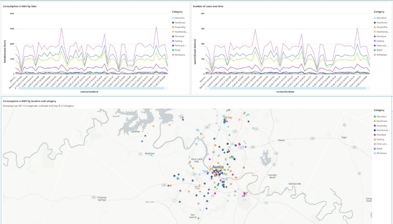
Then, create a dashboard showing energy consumption and number of connected users over time. The dashboard also shows the list of locations on the map by category.

Streaming ingestion benefits

In this section, we discuss some of the benefits of streaming ingestion.

High throughput with low latency

Amazon Redshift can handle and process several gigabytes of data per second from Kinesis Data Streams. (Throughput is dependent on the number of shards in the data stream and the Amazon Redshift cluster configuration.) This allows you to experience low latency and high bandwidth when consuming streaming data, so you can derive insights from your data in seconds instead of minutes.

As we mentioned earlier, the key differentiator with the direct ingestion pull approach in Amazon Redshift is lower latency, which is in seconds. Contrast this to the approach of creating a process to consume the streaming data, staging the data in Amazon S3, and then running a COPY command to load the data into Amazon Redshift. This approach introduces latency in minutes due to the multiple steps involved in processing the data.

Straightforward setup

Getting started is easy. All the setup and configuration in Amazon Redshift uses SQL, which most cloud data warehouse users are already familiar with. You can get real-time insights in seconds without managing complex pipelines. Amazon Redshift with Kinesis Data Streams is fully managed, and you can run your streaming applications without requiring infrastructure management.

Increased productivity

You can perform rich analytics on streaming data within Amazon Redshift and using existing familiar SQL without needing to learn new skills or languages. You can create other materialized views, or views on materialized views, to do most of your ELT data pipeline transforms within Amazon Redshift using SQL.

Streaming ingestion use cases

With near-real time analytics on streaming data, many use cases and industry verticals applications become possible. The following are just some of the many application use cases:

  • Improve the gaming experience – You can focus on in-game conversions, player retention, and optimizing the gaming experience by analyzing real-time data from gamers.
  • Analyze clickstream user data for online advertising – The average customer visits dozens of websites in a single session, yet marketers typically analyze only their own websites. You can analyze authorized clickstream data ingested into the warehouse to assess your customer’s footprint and behavior, and target ads to your customers just-in-time.
  • Real-time retail analytics on streaming POS data – You can access and visualize all your global point of sale (POS) retail sales transaction data for real-time analytics, reporting, and visualization.
  • Deliver real-time application insights – With the ability to access and analyze streaming data from your application log files and network logs, developers and engineers can conduct real-time troubleshooting of issues, deliver better products, and alert systems for preventative measures.
  • Analyze IoT data in real time – You can use Amazon Redshift streaming ingestion with Amazon Kinesis services for real-time applications such as device status and attributes such as location and sensor data, application monitoring, fraud detection, and live leaderboards. You can ingest streaming data using Kinesis Data Streams, process it using Amazon Kinesis Data Analytics, and emit the results to any data store or application using Kinesis Data Streams with low end-to-end latency.

Conclusion

This post showed how to create Amazon Redshift materialized views to ingest data from Kinesis data streams using Amazon Redshift streaming ingestion. With this new feature, you can easily build and maintain data pipelines to ingest and analyze streaming data with low latency and high throughput.

The streaming ingestion preview is now available in all AWS Regions where Amazon Redshift is available. To get started with Amazon Redshift streaming ingestion, provision an Amazon Redshift cluster on the current track and verify your cluster is running version 1.0.35480 or later.

For more information, refer to Streaming ingestion (preview), and check out the demo Real-time Analytics with Amazon Redshift Streaming Ingestion on YouTube.


About the Author

Sam Selvan is a Senior Analytics Solution Architect with Amazon Web Services.

Amazon EMR on Amazon EKS provides up to 61% lower costs and up to 68% performance improvement for Spark workloads

Post Syndicated from Melody Yang original https://aws.amazon.com/blogs/big-data/amazon-emr-on-amazon-eks-provides-up-to-61-lower-costs-and-up-to-68-performance-improvement-for-spark-workloads/

Amazon EMR on Amazon EKS is a deployment option offered by Amazon EMR that enables you to run Apache Spark applications on Amazon Elastic Kubernetes Service (Amazon EKS) in a cost-effective manner. It uses the EMR runtime for Apache Spark to increase performance so that your jobs run faster and cost less.

Amazon EMR on Amazon EKS is a deployment option offered by Amazon EMR that enables you to run Apache Spark applications on Amazon Elastic Kubernetes Service (Amazon EKS) in a cost-effective manner. It uses the EMR runtime for Apache Spark to increase performance so that your jobs run faster and cost less.

In our benchmark tests using TPC-DS datasets at 3 TB scale, we observed that Amazon EMR on EKS provides up to 61% lower costs and up to 68% improved performance compared to running open-source Apache Spark on Amazon EKS via equivalent configurations. In this post, we walk through the performance test process, share the results, and discuss how to reproduce the benchmark. We also share a few techniques to optimize job performance that could lead to further cost-optimization for your Spark workloads.

How does Amazon EMR on EKS reduce cost and improve performance?

The EMR runtime for Spark is a performance-optimized runtime for Apache Spark that is 100% API compatible with open-source Apache Spark. It’s enabled by default with Amazon EMR on EKS. It helps run Spark workloads faster, leading to lower running costs. It includes multiple performance optimization features, such as Adaptive Query Execution (AQE), dynamic partition pruning, flattening scalar subqueries, bloom filter join, and more.

In addition to the cost benefit brought by the EMR runtime for Spark, Amazon EMR on EKS can take advantage of other AWS features to further optimize cost. For example, you can run Amazon EMR on EKS jobs on Amazon Elastic Compute Cloud (Amazon EC2) Spot Instances, providing up to 90% cost savings when compared to On-Demand Instances. Also, Amazon EMR on EKS supports Arm-based Graviton EC2 instances, which creates a 15% performance improvement and up to 30% cost savings when compared a Graviton2-based M6g to M5 instance type.

The recent graceful executor decommissioning feature makes Amazon EMR on EKS workloads more robust by enabling Spark to anticipate Spot Instance interruptions. Without the need to recompute or rerun impacted Spark jobs, Amazon EMR on EKS can further reduce job costs via critical stability and performance improvements.

Additionally, through container technology, Amazon EMR on EKS offers more options to debug and monitor Spark jobs. For example, you can choose Spark History Server, Amazon CloudWatch, or Amazon Managed Prometheus and Amazon Managed Grafana (for more details, refer to the Monitoring and Logging workshop). Optionally, you can use familiar command line tools such as kubectl to interact with a job processing environment and observe Spark jobs in real time, which provides a fail-fast and productive development experience.

Amazon EMR on EKS supports multi-tenant needs and offers application-level security control via a job execution role. It enables seamless integrations to other AWS native services without a key-pair set up in Amazon EKS. The simplified security design can reduce your engineering overhead and lower the risk of data breach. Furthermore, Amazon EMR on EKS handles security and performance patches so you can focus on building your applications.

Benchmarking

This post provides an end-to-end Spark benchmark solution so you can get hands-on with the performance test process. The solution uses unmodified TPC-DS data schema and table relationships, but derives queries from TPC-DS to support the Spark SQL test case. It is not comparable to other published TPC-DS benchmark results.

Key concepts

Transaction Processing Performance Council-Decision Support (TPC-DS) is a decision support benchmark that is used to evaluate the analytical performance of big data technologies. Our test data is a TPC-DS compliant dataset based on the TPC-DS Standard Specification, Revision 2.4 document, which outlines the business model and data schema, relationship, and more. As the whitepaper illustrates, the test data contains 7 fact tables and 17 dimension tables, with an average of 18 columns. The schema consists of essential retailer business information, such as customer, order, and item data for the classic sales channels: store, catalog, and internet. This source data is designed to represent real-world business scenarios with common data skews, such as seasonal sales and frequent names. Additionally, the TPC-DS benchmark offers a set of discrete scaling points (scale factors) based on the approximate size of the raw data. In our test, we chose the 3 TB scale factor, which produces 17.7 billion records, approximately 924 GB compressed data in Parquet file format.

Test approach

A single test session consists of 104 Spark SQL queries that were run sequentially. To get a fair comparison, each session of different deployment types, such as Amazon EMR on EKS, was run three times. The average runtime per query from these three iterations is what we analyze and discuss in this post. Most importantly, it derives two summarized metrics to represent our Spark performance:

  • Total execution time – The sum of the average runtime from three iterations
  • Geomean – The geometric mean of the average runtime

 Test results

In the test result summary (see the following figure), we discovered that the Amazon EMR-optimized Spark runtime used by Amazon EMR on EKS is approximately 2.1 times better than the open-source Spark on Amazon EKS in geometric mean and 3.5 times faster by the total runtime.

The following figure breaks down the performance summary by queries. We observed that EMR runtime for Spark was faster in every query compared to open-source Spark. Query q67 was the longest query in the performance test. The average runtime with open-source Spark was 1019.09 seconds. However, it took 150.02 seconds with Amazon EMR on EKS, which is 6.8 times faster. The highest performance gain in these long-running queries was q72—319.70 seconds (open-source Spark) vs. 26.86 seconds (Amazon EMR on EKS), a 11.9 times improvement.

Test cost

Amazon EMR pricing on Amazon EKS is calculated based on the vCPU and memory resources used from the time you start to download your EMR application Docker image until the Amazon EKS pod terminates. As a result, you don’t pay any Amazon EMR charges until your application starts to run, and you only pay for the vCPU and memory used during a job—you don’t pay for the full amount of compute resources in an EC2 instance.

Overall, the estimated benchmark cost in the US East (N. Virginia) Region is $22.37 per run for open-source Spark on Amazon EKS and $8.70 per run for Amazon EMR on EKS – that’s 61% cheaper due to the 68% quicker job runtime. The following table provides more details.

Benchmark Job Runtime (Hour) Estimated Cost Total EC2 Instance Total vCPU Total Memory (GiB) Root Device (EBS)
Amazon EMR on EKS 0.68 $8.70 6 216 432 20 GiB gp2
Open-Source Spark on Amazon EKS 2.13 $22.37 6 216 432 20 GiB gp2

Amazon EMR on Amazon EC2

(1 primary and 5 core nodes)

0.80 $8.80 6 196 424 20 GiB gp2

The cost estimate doesn’t account for Amazon Simple Storage Service (Amazon S3) storage, or PUT and GET requests. The Amazon EMR on EKS uplift calculation is based on the hourly billing information provided by AWS Cost Explorer.

Cost breakdown

The following is the cost breakdown for the Amazon EMR on EKS job ($8.70): 

  • Total uplift on vCPU – (126.93 * $0.01012) = (total number of vCPU used * per vCPU-hours rate) = $1.28
  • Total uplift on memory – (258.7 * $0.00111125) = (total amount of memory used * per GB-hours rate) = $0.29
  • Total Amazon EMR uplift cost – $1.57
  • Total Amazon EC2 cost – (6 * $1.728 * 0.68) = (number of instances * c5d.9xlarge hourly rate * job runtime in hour) = $7.05
  • Other costs – ($0.1 * 0.68) + ($0.1/730 * 20 * 6 * 0.68) = (shared Amazon EKS cluster charge per hour * job runtime in hour) + (EBS per GB-hourly rate * root EBS size * number of instances * job runtime in hour) = $0.08 

The following is the cost breakdown for the open-source Spark on Amazon EKS job ($22.37): 

  • Total Amazon EC2 cost – (6 * $1.728 * 2.13) = (number of instances * c5d.9xlarge hourly rate * job runtime in hour) = $22.12
  • Other costs – ($0.1 * 2.13) + ($0.1/730 * 20 * 6 * 2.13) = (shared EKS cluster charge per hour * job runtime in hour) + (EBS per GB-hourly rate * root EBS size * number of instances * job runtime in hour) = $0.25

The following is the cost breakdown for the Amazon EMR on Amazon EC2 ($8.80):

  • Total Amazon EMR cost – (5 * $0.27 * 0.80) + (1 * $0.192 * 0.80) = (number of core nodes * c5d.9xlarge Amazon EMR price * job runtime in hour) + (number of primary nodes * m5.4xlarge Amazon EMR price * job runtime in hour) = $1.23
  • Total Amazon EC2 cost – (5 * $1.728 * 0.80) + (1 * $0.768 * 0.80) = (number of core nodes * c5d.9xlarge instance price * job runtime in hour) + (number of primary nodes * m5.4xlarge instance price * job runtime in hour) = $7.53
  • Other Cost – ($0.1/730 * 20 GiB * 6 * 0.80) + ($0.1/730 * 256 GiB * 1 * 0.80) = (EBS per GB-hourly rate * root EBS size * number of instances * job runtime in hour) + (EBS per GB-hourly rate * default EBS size for m5.4xlarge * number of instances * job runtime in hour) = $0.041

Benchmarking considerations

In this section, we share some techniques and considerations for the benchmarking.

Set up an Amazon EKS cluster with Availability Zone awareness

Our Amazon EKS cluster configuration looks as follows:

apiVersion: eksctl.io/v1alpha5
kind: ClusterConfig
metadata:
  name: $EKSCLUSTER_NAME
  region: us-east-1
availabilityZones:["us-east-1a"," us-east-1b"]  
managedNodeGroups: 
  - name: mn-od
    availabilityZones: ["us-east-1b"] 

In the cluster configuration, the mn-od managed node group is assigned to the single Availability Zone b, where we run the test against.

Availability Zones are physically separated by a meaningful distance from other Availability Zones in the same AWS Region. This produces round trip latency between two compute instances located in different Availability Zones. Spark implements distributed computing, so exchanging data between compute nodes is inevitable when performing data joins, windowing, and aggregations across multiple executors. Shuffling data between multiple Availability Zones adds extra latency to the network I/O, which therefore directly impacts Spark performance. Additionally, when data is transferred between two Availability Zones, data transfer charges apply in both directions.

For this benchmark, which is a time-sensitive workload, we recommend running in a single Availability Zone and using On-Demand instances (not Spot) to have a dedicated compute resource. In an existing Amazon EKS cluster, you may have multiple instance types and a Multi-AZ setup. You can use the following Spark configuration to achieve the same goal:

--conf spark.kubernetes.node.selector.eks.amazonaws.com/capacityType=ON_DEMAND
--conf spark.kubernetes.node.selector.topology.kubernetes.io/zone=us-east-1b

Use instance store volume to increase disk I/O

Spark data shuffle, the process of reading and writing intermediate data to disk, is a costly operation. Besides the network I/O speed, Spark demands high performant disk to support a large amount of data redistribution activities. I/O operations per second (IOPS) is an equally important measure to baseline Spark performance. For instance, the SQL queries 23a, 23b, 50, and 93 are shuffle-intensive Spark workloads in TPC-DS, so choosing an optimal storage strategy can significantly shorten their runtime. General speaking, the recommended options are either attaching multiple EBS disk volumes per node in Amazon EKS or using the d series EC2 instance type, which offers high disk I/O performance within a compute family (for example, c5d.9xlarge is the d series in the c5 compute optimized family).

The following table summarizes the hardware specification we used:

Instance On-Demand Hourly Price vCPU Memory (GiB) Instance Store Networking Performance (Gbps) 100% Random Read IOPS Write IOPS
c5d.9xlarge $1.73 36 72 1 x 900GB NVMe SSD 10 350,000 170,000

To simplify our hardware configuration, we chose the AWS Nitro System EC2 instance type c5d.9xlarge, which comes with a NVMe-based SSD instance store volume. As of this writing, the built-in NVMe SSD disk requires less effort to set up and provides optimal disk performance we need. In the following code, the one-off preBoostrapCommand is triggered to mount an instance store to a node in Amazon EKS:

managedNodeGroups: 
  - name: mn-od
    preBootstrapCommands:
      - "sleep 5; sudo mkfs.xfs /dev/nvme1n1;sudo mkdir -p /local1;sudo echo /dev/nvme1n1 /local1 xfs defaults,noatime 1 2 >> /etc/fstab"
      - "sudo mount -a"
      - "sudo chown ec2-user:ec2-user /local1"

Run as a predefined job user, not a root user

For security, it’s not recommended to run Spark jobs as a root user. But how can you access the NVMe SSD volume mounted to the Amazon EKS cluster as a non-root Spark user?

An init container is created for each Spark driver and executor pods in order to set the volume permission and control the data access. Let’s check out the Spark driver pod via the kubectl exec command, which allows us execute into the running container and have an interactive session. We can observe the following:

  • The init container is called volume-permission.
  • The SSD disk is called /ossdata1. The Spark driver has stored some data to the disk.
  • The non-root Spark job user is called hadoop.

This configuration is provided in a format of a pod template file for Amazon EMR on EKS, so you can dynamically tailor job pods when Spark configuration doesn’t support your needs. Be aware that the predefined user’s UID in the EMR runtime for Spark is 999, but it’s set to 1000 in open-source Spark. The following is a sample Amazon EMR on EKS driver pod template:

apiVersion: v1
kind: Pod
spec:
  nodeSelector:
    app: sparktest
  volumes:
    - name: spark-local-dir-1
      hostPath:
        path: /local1  
  initContainers:  
  - name: volume-permission
    image: public.ecr.aws/y4g4v0z7/busybox
    # grant volume access to "hadoop" user with uid 999
    command: ['sh', '-c', 'mkdir /data1; chown -R 999:1000 /data1'] 
    volumeMounts:
      - name: spark-local-dir-1
        mountPath: /data1
  containers:
  - name: spark-kubernetes-driver
    volumeMounts:
      - name: spark-local-dir-1
        mountPath: /data1

In the job submission, we map the pod templates via the Spark configuration:

"spark.kubernetes.driver.podTemplateFile": "s3://'$S3BUCKET'/pod-template/driver-pod-template.yaml",
"spark.kubernetes.executor.podTemplateFile": "s3://'$S3BUCKET'/pod-template/executor-pod-template.yaml",

Spark on k8s operator is a popular tool to deploy Spark on Kubernetes. Our open-source Spark benchmark uses the tool to submit the job to Amazon EKS. However, the Spark operator currently doesn’t support file-based pod template customization, due to the way it operates. So we embed the disk permission setup into the job definition, as in the example on GitHub.

Disable dynamic resource allocation and enable Adaptive Query Execution in your application

Spark provides a mechanism to dynamically adjust compute resources based on workload. This feature is called dynamic resource allocation. It provides flexibility and efficiency to manage compute resources. For example, your application may give resources back to the cluster if they’re no longer used, and may request them again later when there is demand. It’s quite useful when your data traffic is unpredictable and an elastic compute strategy is needed at your application level. While running the benchmarking, our source data volume (3 TB) is certain and the jobs were run on a fixed-size Spark cluster that consists of six EC2 instances. You can turn off the dynamic allocation in EMR on EC2 as shown in the following code, because it doesn’t suit our purpose and might add latency to the test result. The rest of Spark deployment options, such as Amazon EMR on EKS, has the dynamic allocation off by default, so we can ignore these settings.

--conf spark.dynamicAllocation.enabled=false 
--conf spark.shuffle.service.enabled=false

Dynamic resource allocation is a different concept from automatic scaling in Amazon EKS, such as the Cluster Autoscaler. Disabling the dynamic allocation feature only fixes our 6-node Spark cluster size per job, but doesn’t stop the Amazon EKS cluster from expanding or shrinking automatically. It means our Amazon EKS cluster is still able to scale between 1 and 30 EC2 instances, as configured in the following code:

managedNodeGroups: 
  - name: mn-od
    availabilityZones: ["us-east-1b"] 
    instanceType: c5d.9xlarge
    minSize: 1
    desiredCapacity: 1
    maxSize: 30

Spark Adaptive Query Execution (AQE) is an optimization technique in Spark SQL since Spark 3.0. It dynamically re-optimizes the query execution plan at runtime, which supports a variety of optimizations, such as the following:

  • Dynamically switch join strategies
  • Dynamically coalesce shuffle partitions
  • Dynamically handle skew joins

The feature is enabled by default in EMR runtime for Spark, but disabled by default in open-source Apache Spark 3.1.2. To provide the fair comparison, make sure it’s set in the open-source Spark benchmark job declaration:

  sparkConf:
    # Enable AQE
    "spark.sql.adaptive.enabled": "true"
    "spark.sql.adaptive.localShuffleReader.enabled": "true"
    "spark.sql.adaptive.coalescePartitions.enabled": "true"
    "spark.sql.adaptive.skewJoin.enabled": "true"

Walkthrough overview

With these considerations in mind, we run three Spark jobs in Amazon EKS. This helps us compare Spark 3.1.2 performance in various deployment scenarios. For more details, check out the GitHub repository.

In this walkthrough, we show you how to do the following:

  • Produce a 3 TB TPC-DS complaint dataset
  • Run a benchmark job with the open-source Spark operator on Amazon EKS
  • Run the same benchmark application with Amazon EMR on EKS

We also provide information on how to benchmark with Amazon EMR on Amazon EC2.

Prerequisites

Install the following tools for the benchmark test:

Provision resources

The provision script creates the following resources:

  • A new Amazon EKS cluster
  • Amazon EMR on EKS enabler
  • The required AWS Identity and Access Management (IAM) roles
  • The S3 bucket emr-on-eks-nvme-${ACCOUNTID}-${AWS_REGION}, referred to as <S3BUCKET> in the following steps

The provisioning process takes approximately 30 minutes.

  1. Download the project with the following command:
    git clone https://github.com/aws-samples/emr-on-eks-bencharmk.git
    cd emr-on-eks-bencharmk

  2. Create a test environment (change the Region if necessary):
    export EKSCLUSTER_NAME=eks-nvme
    export AWS_REGION=us-east-1
    
    ./provision.sh

Modify the script if needed for testing against an existing Amazon EKS cluster. Make sure the existing cluster has the Cluster Autoscaler and Spark Operator installed. Examples are provided by the script.

  1. Validate the setup:
    # should return results
    kubectl get pod -n oss | grep spark-operator
    kubectl get pod -n kube-system | grep nodescaler

Generate TPC-DS test data (optional)

In this optional task, you generate TPC-DS test data in s3://<S3BUCKET>/BLOG_TPCDS-TEST-3T-partitioned. The process takes approximately 80 minutes.

The job generates TPC-DS compliant datasets with your preferred scale. In this case, it creates 3 TB of source data (approximately 924 GB compressed) in Parquet format. We have pre-populated the source dataset in the S3 bucket blogpost-sparkoneks-us-east-1 in Region us-east-1. You can skip the data generation job if you want to have a quick start.

Be aware of that cross-Region data transfer latency will impact your benchmark result. It’s recommended to generate the source data to your S3 bucket if your test Region is different from us-east-1.

  1. Start the job:
    kubectl apply -f examples/tpcds-data-generation.yaml

  2. Monitor the job progress:
    kubectl get pod -n oss
    kubectl logs tpcds-data-generation-3t-driver -n oss

  3. Cancel the job if needed:
    kubectl delete -f examples/tpcds-data-generation.yaml

The job runs in the namespace oss with a service account called oss in Amazon EKS, which grants a minimum permission to access the S3 bucket via an IAM role. Update the example .yaml file if you have a different setup in Amazon EKS.

Benchmark for open-source Spark on Amazon EKS

Wait until the data generation job is complete, then update the default input location parameter (s3://blogpost-sparkoneks-us-east-1/blog/BLOG_TPCDS-TEST-3T-partitioned) to your S3 bucket in the tpcds-benchmark.yaml file.. Other parameters in the application can also be adjusted. Check out the comments in the yaml file for details. This process takes approximately 130 minutes.

If the data generation job is skipped, run the following steps without waiting.

  1. Start the job:
    kubectl apply -f examples/tpcds-benchmark.yaml

  2. Monitor the job progress:
    kubectl get pod -n oss
    kubectl logs tpcds-benchmark-oss-driver -n oss

  3. Cancel the job if needed:
    kubectl delete -f examples/tpcds-benchmark.yaml

The benchmark application outputs a CSV file capturing runtime per Spark SQL query and a JSON file with query execution plan details. You can use the collected metrics and execution plans to compare and analyze performance between different Spark runtimes (open-source Apache Spark vs. EMR runtime for Spark).

Benchmark with Amazon EMR on EKS

Wait for the data generation job finish before starting the benchmark for Amazon EMR on EKS. Don’t forget to change the input location (s3://blogpost-sparkoneks-us-east-1/blog/BLOG_TPCDS-TEST-3T-partitioned) to your S3 bucket. The output location is s3://<S3BUCKET>/EMRONEKS_TPCDS-TEST-3T-RESULT. If you use the pre-populated TPC-DS dataset, start the Amazon EMR on EKS benchmark without waiting. This process takes approximately 40 minutes.

  1. Start the job (change the Region if necessary):
    export EMRCLUSTER_NAME=emr-on-eks-nvme
    export AWS_REGION=us-east-1
    
    ./examples/emr6.5-benchmark.sh

Amazon EKS offers multi-tenant isolation and optimized resource allocation features, so it’s safe to run two benchmark tests in parallel on a single Amazon EKS cluster.

  1. Monitor the job progress in real time:
    kubectl get pod -n emr
    #run the command then search "execution time" in the log to analyze individual query's performance
    kubectl logs YOUR_DRIVER_POD_NAME -n emr spark-kubernetes-driver

  2. Cancel the job (get the IDs from the cluster list on the Amazon EMR console):
    aws emr-containers cancel-job-run --virtual-cluster-id <YOUR_VIRTUAL_CLUSTER_ID> --id <YOUR_JOB_ID>

The following are additional useful commands:

#Check volume status
kubectl exec -it YOUR_DRIVER_POD_NAME -c spark-kubernetes-driver -n emr -- df -h

#Login to a running driver pod
kubectl exec -it YOUR_DRIVER_POD_NAME -c spark-kubernetes-driver -n emr – bash

#Monitor compute resource usage
watch "kubectl top node"

Benchmark for Amazon EMR on Amazon EC2

Optionally, you can use the same benchmark solution to test Amazon EMR on Amazon EC2. Download the benchmark utility application JAR file from a running Kubernetes container, then submit a job via the Amazon EMR console. More details are available in the GitHub repository.

Clean up

To avoid incurring future charges, delete the resources generated if you don’t need the solution anymore. Run the following cleanup script (change the Region if necessary):

cd emr-on-eks-bencharmk

export EKSCLUSTER_NAME=eks-nvme
export AWS_REGION=us-east-1

./deprovision.sh

Conclusion

Without making any application changes, we can run Apache Spark workloads faster and cheaper with Amazon EMR on EKS when compared to Apache Spark on Amazon EKS. We used a benchmark solution running on a 6-node c5d.9xlarge Amazon EKS cluster and queried a TPC-DS dataset at 3 TB scale. The performance test result shows that Amazon EMR on EKS provides up to 61% lower costs and up to 68% performance improvement over open-source Spark 3.1.2 on Amazon EKS.

If you’re wondering how much performance gain you can achieve with your use case, try out the benchmark solution or the EMR on EKS Workshop. You can also contact your AWS Solution Architects, who can be of assistance alongside your innovation journey.


About the Authors

Melody Yang is a Senior Big Data Solution Architect for Amazon EMR at AWS. She is an experienced analytics leader working with AWS customers to provide best practice guidance and technical advice in order to assist their success in data transformation. Her areas of interests are open-source frameworks and automation, data engineering and DataOps.

Kinnar Kumar Sen is a Sr. Solutions Architect at Amazon Web Services (AWS) focusing on Flexible Compute. As a part of the EC2 Flexible Compute team, he works with customers to guide them to the most elastic and efficient compute options that are suitable for their workload running on AWS. Kinnar has more than 15 years of industry experience working in research, consultancy, engineering, and architecture.

[Security Nation] Whitney Merrill on the Crypto & Privacy Village (and the Latest in Data Privacy)

Post Syndicated from Rapid7 original https://blog.rapid7.com/2022/04/27/security-nation-whitney-merrill-on-the-crypto-privacy-village-and-the-latest-in-data-privacy/

[Security Nation] Whitney Merrill on the Crypto & Privacy Village (and the Latest in Data Privacy)

In this episode of Security Nation, Jen and Tod chat with Whitney Merrill, Data Protection Officer at Asana, about her work on the Crypto & Privacy Village and data privacy more broadly. She talks about how she keeps up with both the excitement and the effort of running the village, a mainstay at DEF CON each year – including the curveballs thrown by COVID-19. Whitney also takes Jen and Tod’s questions about the major data privacy topics of the day, touching on everything from vaccine passports to new legislation in California, targeted advertising, and the overlap between security and privacy.

Stick around for our Rapid Rundown, where Tod and Jen talk about psychic signatures in Java – which doesn’t involve ghosts, but does involve Dr. Who.

Whitney Merrill

[Security Nation] Whitney Merrill on the Crypto & Privacy Village (and the Latest in Data Privacy)

Whitney Merrill is Asana’s Data Protection Officer and heads up the growing privacy team. Previously she was Privacy, eCommerce & Consumer Protection Counsel at Electronic Arts (EA) and an attorney at the Federal Trade Commission. In her spare time, she runs the Crypto & Privacy Village, a nonprofit, which appears at DEF CON & BSidesSF each year.

Show notes

Interview links

Rapid Rundown links

Like the show? Want to keep Jen and Tod in the podcasting business? Feel free to rate and review with your favorite podcast purveyor, like Apple Podcasts.

Want More Inspiring Stories From the Security Community?

Subscribe to Security Nation Today

Cloudflare blocks 15M rps HTTPS DDoS attack

Post Syndicated from Omer Yoachimik original https://blog.cloudflare.com/15m-rps-ddos-attack/

Cloudflare blocks 15M rps HTTPS DDoS attack

Cloudflare blocks 15M rps HTTPS DDoS attack

Earlier this month, Cloudflare’s systems automatically detected and mitigated a 15.3 million request-per-second (rps) DDoS attack — one of the largest HTTPS DDoS attacks on record.

While this isn’t the largest application-layer attack we’ve seen, it is the largest we’ve seen over HTTPS. HTTPS DDoS attacks are more expensive in terms of required computational resources because of the higher cost of establishing a secure TLS encrypted connection. Therefore it costs the attacker more to launch the attack, and for the victim to mitigate it. We’ve seen very large attacks in the past over (unencrypted) HTTP, but this attack stands out because of the resources it required at its scale.

The attack, lasting less than 15 seconds, targeted a Cloudflare customer on the Professional (Pro) plan operating a crypto launchpad. Crypto launchpads are used to surface Decentralized Finance projects to potential investors. The attack was launched by a botnet that we’ve been observing — we’ve already seen large attacks as high as 10M rps matching the same attack fingerprint.

Cloudflare customers are protected against this botnet and do not need to take any action.

Cloudflare blocks 15M rps HTTPS DDoS attack

The attack

What’s interesting is that the attack mostly came from data centers. We’re seeing a big move from residential network Internet Service Providers (ISPs) to cloud compute ISPs.

This attack was launched from a botnet of approximately 6,000 unique bots. It originated from 112 countries around the world. Almost 15% of the attack traffic originated from Indonesia, followed by Russia, Brazil, India, Colombia, and the United States.

Cloudflare blocks 15M rps HTTPS DDoS attack

Within those countries, the attack originated from over 1,300 different networks. The top networks included the German provider Hetzner Online GmbH (Autonomous System Number 24940), Azteca Comunicaciones Colombia (ASN 262186), OVH in France (ASN 16276), as well as other cloud providers.

Cloudflare blocks 15M rps HTTPS DDoS attack

How this attack was automatically detected and mitigated

To defend organizations against DDoS attacks, we built and operate software-defined systems that run autonomously. They automatically detect and mitigate DDoS attacks across our entire network — and just as in this case, the attack was automatically detected and mitigated without any human intervention.

Our system starts by sampling traffic asynchronously; it then analyzes the samples and applies mitigations when needed.

Sampling

Initially, traffic is routed through the Internet via BGP Anycast to the nearest Cloudflare data centers that are located in over 250 cities around the world. Once the traffic reaches our data center, our DDoS systems sample it asynchronously allowing for out-of-path analysis of traffic without introducing latency penalties.

Analysis and mitigation

The analysis is done using data streaming algorithms. HTTP request samples are compared to conditional fingerprints, and multiple real-time signatures are created based on dynamic masking of various request fields and metadata. Each time another request matches one of the signatures, a counter is increased. When the activation threshold is reached for a given signature, a mitigation rule is compiled and pushed inline. The mitigation rule includes the real-time signature and the mitigation action, e.g. block.

Cloudflare customers can also customize the settings of the DDoS protection systems by tweaking the HTTP DDoS Managed Rules.

You can read more about our autonomous DDoS protection systems and how they work in our deep-dive technical blog post.

Helping build a better Internet

At Cloudflare, everything we do is guided by our mission to help build a better Internet. The DDoS team’s vision is derived from this mission: our goal is to make the impact of DDoS attacks a thing of the past. The level of protection that we offer is unmetered and unlimited — It is not bounded by the size of the attack, the number of the attacks, or the duration of the attacks. This is especially important these days because as we’ve recently seen, attacks are getting larger and more frequent.

Not using Cloudflare yet? Start now with our Free and Pro plans to protect your websites, or contact us for comprehensive DDoS protection for your entire network using Magic Transit.

Security updates for Wednesday

Post Syndicated from original https://lwn.net/Articles/892802/

Security updates have been issued by Mageia (virtualbox), Red Hat (container-tools:2.0, container-tools:3.0, gzip, kernel, kernel-rt, kpatch-patch, mariadb:10.3, mariadb:10.5, maven-shared-utils, polkit, vim, xmlrpc-c, and zlib), Scientific Linux (maven-shared-utils), SUSE (ant, go1.17, go1.18, kernel, and xen), and Ubuntu (fribidi, git, libcroco, libsepol, linux, linux-gcp, linux-ibm, linux-lowlatency, openjdk-17, and openjdk-lts).

Registering SMS Sender IDs in Singapore

Post Syndicated from Brent Meyer original https://aws.amazon.com/blogs/messaging-and-targeting/registering-sms-sender-ids-in-singapore/

A few weeks ago, we published a blog post about the process of registering alphanumeric Sender IDs. Today, we’re announcing support for registering Sender IDs in Singapore.

About Sender ID registration in Singapore

Singapore’s Infocomm Media Development Authority (IMDA) has created a Sender ID registry to protect consumers from fraudulent and malicious SMS messages. This registry is called the Singapore SMS Sender ID Registry (SSIR).

The government of Singapore encourages all government agencies and financial institutions to register with SSIR. Organizations and businesses outside of these industries can also register with SSIR.

Currently, there is no requirement to register your Sender ID. However, when you register with the SSIR, your Sender ID becomes a “Protected Sender ID.” Protected Sender IDs help to protect you and your customers by preventing other senders from using your Sender ID.

Note that in order to complete this registration process, your business or organization must have a Unique Entity Number (UEN). Businesses and other organizations receive a UEN when they register with Singapore’s Accounting and Corporate Regulatory Authority.

Registering your Sender ID

The first step in the registration process is to create a Protected Sender ID through the Singapore Network Information Centre (SGNIC). To initiate the registration process, send an email to [email protected]. In your message, include the name of your business, the Sender IDs that you want to register, and a description of your use case. SGNIC may contact you for additional information.

After you register with SGNIC, open a ticket in the AWS Support Center. You can find the procedure for opening a case in the Amazon Pinpoint User Guide. The AWS Support team will respond to your case within 24 hours. Their response includes a template for a letter that shows your intent to register a Sender ID.

The next step is to modify the contents of this letter. The regulatory groups in Singapore require a copy of this letter in order to allow AWS to send messages using your Sender ID. Begin by placing the contents of the letter on your company’s letterhead. Next, modify the fields that are highlighted in yellow. These fields include the following:

  • <Place>: The address of your company or organization.
  • <Brand Owner Company Name>: The name of your company or organization.
  • <Number>: Your Unique Entity Number.
  • <Signature>, <Name>, <Title>: The personal signature, name, and job title of the person who is submitting the request on behalf of your company or organization.
  • <ExampleSenderId1>, <ExampleSenderId2>: The Sender IDs that you intend to register with SGNIC. You can add or remove lines here depending on how many Sender IDs you plan to register.

Once you finish modifying the letter, submit it by attaching it to your existing case in the AWS Support Center.

What happens next?

IMDA regularly sends us lists of new Sender ID registrations. When we receive confirmation that your Sender ID has been registered, we update your account to allow it to send SMS messages through your Sender ID. We will also comment on your Support case to indicate that the process is complete.

Wrapping up

We continue to monitor changes to Sender ID registration requirements around the world. We’re working closely with carriers and organizations around the world to make the registration processes as straightforward as possible for our customers. Check in on this blog regularly to learn more about future regulatory changes.

For more information about registering Sender IDs in Singapore, see Special requirements for Singapore in the Amazon Pinpoint User Guide.

[$] Super Python (part 2)

Post Syndicated from original https://lwn.net/Articles/892080/

Python’s super()
built-in function
can be somewhat confusing, as highlighted by a huge
python-ideas thread that we started looking
at
last week. It is used by methods in class hierarchies to access
methods and attributes in a parent class, but exactly which class
that super() resolves to is perhaps a bit unclear in multiple-inheritance hierarchies.
The discussion in the second “half” of the thread further highlighted some
lesser-known parts of the language.

Testing my System Code in /usr/ Without Modifying /usr/

Post Syndicated from original https://0pointer.net/blog/testing-my-system-code-in-usr-without-modifying-usr.html

I recently
blogged

about how to run a volatile systemd-nspawn container from your
host’s /usr/ tree, for quickly testing stuff in your host
environment, sharing your home drectory, but all that without making a
single modification to your host, and on an isolated node.

The one-liner discussed in that blog story is great for testing during
system software development. Let’s have a look at another systemd
tool that I regularly use to test things during systemd development,
in a relatively safe environment, but still taking full benefit of my
host’s setup.

Since a while now, systemd has been shipping with a simple component
called
systemd-sysext. It’s
primary usecase goes something like this: on one hand OS systems with
immutable /usr/ hierarchies are fantastic for security, robustness,
updating and simplicity, but on the other hand not being able to
quickly add stuff to /usr/ is just annoying.

systemd-sysext is supposed to bridge this contradiction: when
invoked it will merge a bunch of “system extension” images into
/usr/ (and /opt/ as a matter of fact) through the use of read-only
overlayfs, making all files shipped in the image instantly and
atomically appear in /usr/ during runtime — as if they always had
been there. Now, let’s say you are building your locked down OS, with
an immutable /usr/ tree, and it comes without ability to log into,
without debugging tools, without anything you want and need when
trying to debug and fix something in the system. With systemd-sysext
you could use a system extension image that contains all this, drop it
into the system, and activate it with systemd-sysext so that it
genuinely extends the host system.

(There are many other usecases for this tool, for example, you could
build systems that way that at their base use a generic image, but by
installing one or more system extensions get extended to with
additional more specific functionality, or drivers, or similar. The
tool is generic, use it for whatever you want, but for now let’s not
get lost in listing all the possibilites.)

What’s particularly nice about the tool is that it supports
automatically discovered dm-verity images, with signatures and
everything. So you can even do this in a fully authenticated,
measured, safe way. But I am digressing…

Now that we (hopefully) have a rough understanding what
systemd-sysext is and does, let’s discuss how specficially we can
use this in the context of system software development, to safely use
and test bleeding edge development code — built freshly from your
project’s build tree – in your host OS without having to risk that the
host OS is corrupted or becomes unbootable by stuff that didn’t quite
yet work the way it was envisioned:

The images systemd-sysext merges into /usr/ can be of two kinds:
disk images with a file system/verity/signature, or simple, plain
directory trees. To make these images available to the tool, they can
be placed or symlinked into /usr/lib/extensions/,
/var/lib/extensions/, /run/lib/extensions/ (and a bunch of
others). So if we now install our freshly built development software
into a subdirectory of those paths, then that’s entirely sufficient to
make them valid system extension images in the sense of
systemd-sysext, and thus can be merged into /usr/ to try them out.

To be more specific: when I develop systemd itself, here’s what I do
regularly, to see how my new development version would behave on my
host system. As preparation I checked out the systemd development git
tree first of course, hacked around in it a bit, then built it with
meson/ninja. And now I want to test what I just built:

sudo DESTDIR=/run/extensions/systemd-test ninja -C build install &&
        sudo systemd-sysext refresh --force

Explanation: first, we’ll install my current build tree as a system
extension into /run/extensions/systemd-test/. And then we apply it
to the host via the systemd-sysext refresh command. This command
will search for all installed system extension images in the
aforementioned directories, then unmount (i.e. “unmerge”) any
previously merged dirs from /usr/ and then freshly mount
(i.e. “merge”) the new set of system extensions on top of /usr/. And
just like that, I have installed my development tree of systemd into
the host OS, and all that without actually modifying/replacing even a
single file on the host at all. Nothing here actually hit the disk!

Note that all this works on any system really, it is not necessary
that the underlying OS even is designed with immutability in
mind. Just because the tool was developed with immutable systems in
mind it doesn’t mean you couldn’t use it on traditional systems where
/usr/ is mutable as well. In fact, my development box actually runs
regular Fedora, i.e. is RPM-based and thus has a mutable /usr/
tree. As long as system extensions are applied the whole of /usr/
becomes read-only though.

Once I am done testing, when I want to revert to how things were without the image installed, it is sufficient to call:

sudo systemd-sysext unmerge

And there you go, all files my development tree generated are gone
again, and the host system is as it was before (and /usr/ mutable
again, in case one is on a traditional Linux distribution).

Also note that a reboot (regardless if a clean one or an abnormal
shutdown) will undo the whole thing automatically, since we installed
our build tree into /run/ after all, i.e. a tmpfs instance that is
flushed on boot. And given that the overlayfs merge is a runtime
thing, too, the whole operation was executed without any
persistence. Isn’t that great?

(You might wonder why I specified --force on the systemd-sysext
refresh
line earlier. That’s because systemd-sysext actually does
some minimal version compatibility checks when applying system
extension images. For that it will look at the host’s
/etc/os-release file with
/usr/lib/extension-release.d/extension-release.<name>, and refuse
operaton if the image is not actually built for the host OS
version. Here we don’t want to bother with dropping that file in
there, we know already that the extension image is compatible with
the host, as we just built it on it. --force allows us to skip the
version check.)

You might wonder: what about the combination of the idea from the
previous blog story (regarding running container’s off the host
/usr/ tree) with system extensions? Glad you asked. Right now we
have no support for this, but it’s high on our TODO list (patches
welcome, of course!). i.e. a new switch for systemd-nspawn called
--system-extension= that would allow merging one or more such
extensions into the container tree booted would be stellar. With that,
with a single command I could run a container off my host OS but with
a development version of systemd dropped in, all without any
persistence. How awesome would that be?

(Oh, and in case you wonder, all of this only works with distributions
that have completed the /usr/ merge. On legacy distributions that
didn’t do that and still place parts of /usr/ all over the hierarchy
the above won’t work, since merging /usr/ trees via overlayfs is
pretty pointess if the OS is not hermetic in /usr/.)

And that’s all for now. Happy hacking!

Evolution of ML Fact Store

Post Syndicated from Netflix Technology Blog original https://netflixtechblog.com/evolution-of-ml-fact-store-5941d3231762

by Vivek Kaushal

At Netflix, we aim to provide recommendations that match our members’ interests. To achieve this, we rely on Machine Learning (ML) algorithms. ML algorithms can be only as good as the data that we provide to it. This post will focus on the large volume of high-quality data stored in Axion — our fact store that is leveraged to compute ML features offline. We built Axion primarily to remove any training-serving skew and make offline experimentation faster. We will share how its design has evolved over the years and the lessons learned while building it.

Terminology

Axion fact store is part of our Machine Learning Platform, the platform that serves machine learning needs across Netflix. Figure 1 below shows how Axion interacts with Netflix’s ML platform. The overall ML platform has tens of components, and the diagram below only shows the ones that are relevant to this post. To understand Axion’s design, we need to know the various components that interact with it.

Figure 1: Netflix ML Architecture
  • Fact: A fact is data about our members or videos. An example of data about members is the video they had watched or added to their My List. An example of video data is video metadata, like the length of a video. Time is a critical component of Axion — When we talk about facts, we talk about facts at a moment in time. These facts are managed and made available by services like viewing history or video metadata services outside of Axion.
  • Compute application: These applications generate recommendations for our members. They fetch facts from respective data services, run feature encoders to generate features and score the ML models to eventually generate recommendations.
  • Offline feature generator: We regenerate the values of the features that were generated for inferencing in the compute application. Offline Feature Generator is a spark application that enables on-demand generation of features using new, existing, or updated feature encoders.
  • Shared feature encoders: Feature encoders are shared between compute applications and offline feature generators. We make sure there is no training/serving skew by using the same data and the code for online and offline feature generation.

Motivation

Five years ago, we posted and talked about the need for a ML fact store. The motivation has not changed since then; the design has. This post focuses on the new design, but here is a summary of why we built this fact store.

Our machine learning models train on several weeks of data. Thus, if we want to run an experiment with a new or modified feature encoder, we need to build several weeks of feature data with this new or modified feature encoder. We have two options to collect features using this updated feature encoder.

The first is to log features from the compute applications, popularly known as feature logging. We can deploy updated feature encoders in our compute applications and then wait for them to log the feature values. Since we train our models on several weeks of data, this method is slow for us as we will have to wait for several weeks for the data collection.

An alternative to feature logging is to regenerate the features with updated feature encoders. If we can access the historical facts, we can regenerate the features using updated feature encoders. Regeneration takes hours compared to weeks taken by the feature logging. Thus, we decided to go this route and started storing facts to reduce the time it takes to run an experiment with new or modified features.

Design evolution

Axion fact store has four components — fact logging client, ETL, query client, and data quality infrastructure. We will describe how the design evolved in these components.

Evolution of Fact Logging Client

Compute applications access facts (members’ viewing history, their likes and my list information, etc.) from various grpc services that power the whole Netflix experience. These facts are used to generate features using shared feature encoders, which in turn are used by ML models to generate recommendations. After generating the recommendations, compute applications use Axion’s fact logging client to log these facts.

At a later stage in the offline pipelines, the offline feature generator uses these logged facts to regenerate temporally accurate features. Temporal accuracy, in this context, is the ability to regenerate the exact set of features that were generated for the recommendations. This temporal accuracy of features is key to removing the training-serving skew.

The first version of our logger library optimized for storage by deduplicating facts and optimized for network i/o using different compression methods for each fact. Then we started hitting roadblocks while optimizing the query performance. Since we were optimizing at the logging level for storage and performance, we had less data and metadata to play with to optimize the query performance.

Eventually, we decided to simplify the logger. Now we asynchronously collect all the facts and metadata into a protobuf, compress it, and send it to the keystone messaging service.

Evolution of ETL and Query Client

ETL and Query Client are intertwined, as any ETL changes could directly impact the query performance. ETL is the component where we experiment for query performance, improving data quality, and storage optimization. Figure 2 shows components of Axion’s ETL and its interaction with the query client.

Fig 2: Internal components of Axion

Axion’s fact logging client logs facts to the keystone real-time stream processing platform, which outputs data to an Iceberg table. We use Keystone as it is easy to use, reliable, scalable, and provides aggregation of facts from different cloud regions into a single AWS region. Having all data in a single AWS region exposes us to a single point of failure but it significantly reduces the operational overhead of our ETL pipelines which we believe makes it a worthwhile trade-off. We currently send all the facts into a single Keystone stream which we have configured to write to a single Iceberg table. We plan to split these Keystone streams into multiple streams for horizontal scalability.

The Iceberg table created by Keystone contains large blobs of unstructured data. These large unstructured blogs are not efficient for querying, so we need to transform and store this data in a different format to allow efficient queries. One might think that normalizing it would make storage and querying more efficient, albeit at the cost of writing more complex queries. Hence, our first approach was to normalize the incoming data and store it in multiple tables. We soon realized that, while space-optimized, it made querying very inefficient for the scale of data we needed to handle. We ran into various shuffle issues in Spark as we were joining several big tables at query time.

We then decided to denormalize the data and store all facts and metadata in one Iceberg table using nested Parquet format. While storing in one Iceberg table was not as space-optimized, Parquet did provide us with significant savings in storage costs, and most importantly, it made our Spark queries succeed. However, Spark query execution remained slow. Further attempts to optimize query performance, like using bloom filters and predicate pushdown, were successful but still far away from where we wanted it to be.

Why was querying the single Iceberg table slow?

What’s our end goal? We want to train our ML models to personalize the member experience. We have a plethora of ML models that drive personalization. Each of these models are trained with different datasets and features along with different stratification and objectives. Given that Axion is used as the defacto Fact store for assembling the training dataset for all these models, it is important for Axion to log and store enough facts that would be sufficient for all these models. However, for a given ML model, we only require a subset of the data stored in Axion for its training needs. We saw queries filtering down an input dataset of several hundred million rows to less than a million in extreme cases. Even with bloom filters, the query performance was slow because the query was downloading all of the data from s3 and then dropping it. As our label dataset was also random, presorting facts data also did not help.

We realized that our options with Iceberg were limited if we only needed data for a million rows — out of several hundred million — and we had no additional information to optimize our queries. So we decided not to further optimize joins with the Iceberg data and instead move to an alternate approach.

Low-latency Queries

To avoid downloading all of the fact data from s3 in a spark executor and then dropping it, we analyzed our query patterns and figured out that there is a way to only access the data that we are interested in. This was achieved by introducing an EVCache, a key-value store, which stores facts and indices optimized for these particular query patterns.

Let’s see how the solution works for one of these query patterns — querying by member id. We first query the index by member id to find the keys for the facts of that member and query those facts from EVCache in parallel. So, we make multiple calls to the key-value store for each row in our training set. Even when accounting for these multiple calls, the query performance is an order of magnitude faster than scanning several hundred times more data stored in the Iceberg table. Depending on the use case, EVCache queries can be 3x-50x faster than Iceberg.

The only problem with this approach is that EVCache is more expensive than Iceberg storage, so we need to limit the amount of data stored. So, for the queries that request data not available in EVCache, our only option is to query Iceberg. In the future, we want to store all facts in EVCache by optimizing how we store data in EVCache.

How do we monitor the quality of data?

Over the years, we learned the importance of having comprehensive data quality checks for our datasets. Corruption in data can significantly impact production model performance and A/B test results. From the ML researchers’ perspective, it doesn’t matter if Axion or a component outside of Axion corrupted the data. When they read the data from Axion, if it is bad, it is a loss of trust in Axion. For Axion to become the defacto fact store for all Personalization ML models, the research teams needed to trust the quality of data stored. Hence, we designed a comprehensive system that monitors the quality of data flowing through Axion to detect corruptions, whether introduced by Axion or outside Axion.

We bucketed data corruptions observed when reading data from Axion on three dimensions:

  • The impact on a value in data: Was the value missing? Did a new value appear (unintentionally)? Was the value replaced with a different value?
  • The spread of data corruption: Did data corruption have a row or columnar impact? Did the corruption impact one pipeline or multiple ML pipelines?
  • The source of data corruption: Was data corrupted by components outside of Axion? Did Axion components corrupt data? Was data corrupted at rest?

We came up with three different approaches to detect data corruption, wherein each approach can detect corruption along multiple dimensions described above.

Aggregations

Data volume logged to Axion datastore is predictable. Compute applications follow daily trends. Some log consistently every hour, others log for a few hours every day. We aggregate the counts on dimensions like total records, compute application, fact counts etc. Then we use a rule-based approach to validate the counts are within a certain threshold of past trends. Alerts are triggered when counts vary outside these thresholds. These trend-based alerts are helpful with missing or new data; row-level impact, and pipelines impact. They help with column-level impact only on rare occasions.

Consistent sampling

We sample a small percentage of the data based on a predictable member id hash and store it in separate tables. By consistent sampling across different data stores and pipelines, we can run canaries on this smaller subset and get output quickly. We also compare the output of these canaries against production to detect unintended changes in data during new code deployment. One downside of consistent sampling is that it may not catch rare issues, especially if the rate of data corruption is significantly lower than our sampling rate. Consistent sampling checks help detect attribute impact — new, missing, or replacement; columnar impact, and single pipeline issues.

Random sampling

While the above two strategies combined can detect most data corruptions, they do occasionally miss. For those rare occasions, we rely on random sampling. We randomly query a subset of the data multiple times every hour. Both hot and cold data, i.e., recently logged data and data logged a while ago, are randomly sampled. We expect these queries to pass without issues. When they fail, it is either due to bad data or issues with the underlying infrastructure. While we think of it as an “I’m feeling lucky” strategy, it does work as long as we read significantly more data than the rate of corrupted data.

Another advantage to random sampling is maintaining the quality of unused facts. Axion users do not read a significant percentage of facts logged to Axion, and we need to make sure that these unused facts are of good quality as they can be used in the future. We have pipelines that randomly read these unused facts and alert when the query does not get the expected output. In terms of impact, these random checks are like winning a lottery — you win occasionally, and you never know how big it is.

Results from monitoring data quality

We deployed the above three monitoring approaches more than two years ago, and since then, we have identified more than 95% of data issues early. We have also significantly improved the stability of our customer pipelines. If you want to know more about how we monitor data quality in Axion, you can check our spark summit talk and this podcast.

Learnings from Axion’s evolution

We learned from designing this fact store to start with a simple design and avoid premature optimizations that add complexity. Pay the storage, network, and compute cost. As the product becomes available to the customers, new use cases will pop up that will be harder to support with a complex design. Once the customers have adopted the product, start looking into optimizations.

While “keep the design simple” is a frequently shared learning in software engineering, it is not always easy to achieve. For example, we learned that our fact logging client can be simple with minimal business logic, but our query client needs to be functionality-rich. Our learning is that if we need to add complexity, add it in the least number of components instead of spreading it out.

Another learning is that we should have invested early into a robust testing framework. Unit tests and integration tests only took us so far. We needed scalability testing and performance testing as well. This scalability and performance testing framework helped stabilize the system because, without it, we ran into issues that took us weeks to clean up.

Lastly, we learned that we should run data migrations and push the breaking API changes as soon as possible. As more customers adopt Axion, running data migrations and making breaking API changes are becoming harder and harder.

Conclusion and future work

Axion is our primary data source that is used extensively by all our Personalization ML models for offline feature generation. Given that it ensures that there is no training/serving skew and that it has significantly reduced offline feature generation latencies we are now starting to make it the defacto Fact store for other ML use cases within Netflix.

We do have use cases that are not served well with the current design, like bandits, because our current design limits storing a map per row creating a limitation when a compute application needs to log multiple values for the same key. Also, as described in the design, we want to optimize how we store data in EVCache to enable us to store more data.

If you are interested in working on similar challenges, join us.


Evolution of ML Fact Store was originally published in Netflix TechBlog on Medium, where people are continuing the conversation by highlighting and responding to this story.

Two voting days, a debate and a polling rule in France impacts the Internet

Post Syndicated from João Tomé original https://blog.cloudflare.com/french-elections-2022-runoff/

Two voting days, a debate and a polling rule in France impacts the Internet

Two voting days, a debate and a polling rule in France impacts the Internet

We blogged previously about some trends concerning the first round of the 2022 French presidential election, held on April 10. Here we take a look at the run-off election this Sunday, April 24, that ended up re-electing Emmanuel Macron as President of France.

First, the two main trends: French-language news sites outside France were clearly impacted by the local rule that states that exit polls can only be published after 20:00.

And Internet traffic was similar on both the election days (April 10 and 24) and that includes the increase in use of mobile devices and interest in news websites — there we also saw a clear interest in the Macron-Le Pen debate on April 20.

We have discussed before that election days usually don’t have a major impact on overall Internet traffic. Let’s compare April 10 with 24, the two Sundays when the elections were held. The trends throughout the day are incredibly similar (with a slight increase in traffic on April 24), even with a two-week gap between them.

Two voting days, a debate and a polling rule in France impacts the Internet

Another election-day trend is the use of mobile devices to access the Internet, mainly at night. The largest spikes in number of requests made using mobile devices in France during April seemed to be all election-related:

Two voting days, a debate and a polling rule in France impacts the Internet

#1. April 10 (first round of the election), 21:00 local time. 58% of traffic by mobile devices.

#2. April 24 (second round of the  election), 22:00. 57% mobile traffic.

#3. April 20 (presidential debate), 22:00. 56% mobile traffic.

Not only did both the election Sundays (after the polling stations were closed) have an impact on mobile traffic in France, but the presidential debate (Wednesday, April 20) had the same type of impact, increasing requests from mobile devices.

The TV debate was seen by 15.6 million viewers in France and lasted between 21:00 and 22:45, local time; at the same time mobile traffic was higher than in any other Wednesday and was the #3 spike of April, with 10% more mobile requests than in the previous Wednesday at the same time.

The special case of French-language news sites

For the elections, local rules state that French media is barred from publishing partial results or polls of any kind until 20:00, the time when voting stations in metropolitan France officially close. So, that means that French news outlets have to wait for the allotted hour to give official projections.

Given that, we looked at French-language news websites from French-speaking countries like Switzerland and Belgium. They aren’t bound by French law and can show information about exit polls earlier (bear in mind that in most French cities polling stations close at 19:00 and only in the bigger cities does it go on until 20:00).

For example, the Swiss Le Temps published exit polls at 19:30.

Two voting days, a debate and a polling rule in France impacts the Internet

We can clearly see that requests to French-language news sites outside France clearly spiked earlier than those in France. News websites in France had spikes after 20:00 local time on both elections days, but Belgian and Swiss news sites had major increases in traffic at 19:00 on April 10 (1857% more than the previous Sunday!). For the runoff elections on April 24, the biggest spike of the month was at 18:00 (3100% more requests than the previous Sunday), but it was also higher than on previous days one hour later, at 19:00 (3080% higher).

There are no spikes at all related to the French debate (April 20), so that seems to show that those Belgian and Swiss news sites had a huge increase of French citizens eager to see the polls before 20:00.

Election results change online patterns

We saw two weeks ago that official election websites had a clear spike in requests on April 10, the first round of the elections. Here we’re looking at DNS request trends to get a sense of traffic to Internet properties.

Official French election-related websites had an increase in traffic throughout the week prior to the first round, after Monday, April 4, but it’s no surprise that the two major spikes were on both the elections’ day. How much? Here is the breakdown by bigger spikes in traffic:

Two voting days, a debate and a polling rule in France impacts the Internet

#1. April 10 (first round of the election), 00:00 local time. 925% more requests than the previous Sunday (at the same time).

#2. April 24  (second round of the election), 20:00. 707% more requests.

#3. April 10 (first round of the election), 20:00. 370% more requests.

#3. April 11, 10:00. 115% more requests than the previous Monday.

(there’s a draw at these last two spikes)

News sites go up after polling stations close

Regarding the main French news websites, as we saw two weeks ago, 20:00 local time, after the polling stations are all closed, and the first major polls are revealed continues to be the time of the biggest spikes of the whole month.

The biggest spike of the month in our aggregate DNS chart, that shows trends from 12 news websites, was definitely on April 10, the first round election day, around 20:00 local time, when those domains had 116% more traffic than at the same time on the previous Sunday. And the second-biggest spike was the runoff election day, on April 24, at the same time (20:00 local time), with an increase of 142% in traffic compared to the previous Sunday at the same time.

Two voting days, a debate and a polling rule in France impacts the Internet

Very close to those two spikes is Monday morning, April 11, after the first round of the elections. At 10:00 local time requests were 45% higher than in the previous Monday. The Macron-Le Pen debate on Wednesday, April 20, also had a spike. At 21:00, when it was starting, requests were 56% higher than on the previous Wednesday.

The same trend is seen on the major French TV station websites, with a clear isolated spike on April 10 (the first round election day) at 20:00 local time, with a 472% increase in traffic compared to the previous Sunday, when the main exit polls were announced. Something similar, at the same time (20:00), on April 24, with a 375% increase in requests compared to the previous Sunday.

Two voting days, a debate and a polling rule in France impacts the Internet

That’s only matched, again, by the April 20 debate. At 21:00 traffic was 308% higher than the previous Wednesday, so people were clearly taking notice of the debate and checking news outlets and TV station websites — there were French sites like france.tv that transmitted via streaming.

Conclusion

When people are really eager to see something as important as election results, they go and search where the first polls are (in this case, before 20:00 local time, they are outside France).

Also, in two different election moments in France separated by two weeks, there are clear similarities in Internet trends that show the way people use the Internet during election periods. That’s more clear when results start to arrive, but also a debate as important for a presidential election as the Le Pen-Macron one, also impacts not only the Internet traffic but also the attention to news and TV websites.

You can keep an eye on these trends using Cloudflare Radar.

Deux jours de vote, un débat et une réglementation concernant les élections en France impactent l’Internet

Post Syndicated from João Tomé original https://blog.cloudflare.com/french-elections-2022-runoff-fr-fr/

Deux jours de vote, un débat et une réglementation concernant les élections en France impactent l'Internet

Deux jours de vote, un débat et une réglementation concernant les élections en France impactent l'Internet

Nous avons publié un article de blog consacré à certaines tendances concernant le premier tour de l’élection présidentielle française de 2022, qui s’est déroulé le 10 avril. Nous nous intéressons ici au second tour de l’élection, qui a eu lieu le dimanche 24 avril et a abouti à la réélection d’Emmanuel Macron à la présidence de la France.

Tout d’abord, les deux principales tendances : les sites d’information francophones situés hors de France ont été clairement impactés par la réglementation locale, qui stipule que les estimations ne peuvent être publiées qu’après 20 heures.

Le trafic Internet a été similaire les deux jours de l’élection (les 10 et 24 avril), et cela inclut l’augmentation de l’utilisation des appareils mobiles et l’intérêt pour les sites d’actualités – – là aussi, nous avons constaté un net intérêt pour le débat Macron-Le Pen du 20 avril.

Nous avons déjà évoqué le fait que les jours d’élections n’ont généralement pas un impact majeur sur le trafic Internet global. Comparons les journées des 10 et 24 avril, les deux dimanches où ont eu lieu les élections. Les tendances tout au long de la journée sont incroyablement similaires (avec une légère augmentation du trafic le 24 avril), même à deux semaines d’intervalle.

Deux jours de vote, un débat et une réglementation concernant les élections en France impactent l'Internet

Une autre tendance des jours d’élection est l’utilisation d’appareils mobiles pour accéder à l’internet, principalement la nuit. Les plus importants pics du nombre de requêtes transmises depuis des appareils mobiles en France au mois d’avril semblent être tous liés aux élections :

Deux jours de vote, un débat et une réglementation concernant les élections en France impactent l'Internet

N°1. 10 avril (premier tour de l’élection), 21 heures, heure locale. 58 % du trafic provenait d’appareils mobiles.

N°2. 24 avril (deuxième tour de l’élection), 22 heures. 57 % de trafic mobile.

N°3. 20 avril (débat présidentiel), 22 heures. 56 % de trafic mobile.

Les deux dimanches de l’élection (après la fermeture des bureaux de vote) ont eu un impact sur le trafic mobile en France, et le débat présidentiel (mercredi 20 avril) a eu un impact semblable, entraînant une augmentation des requêtes provenant d’appareils mobiles.

Le débat télévisé a été regardé par 15,6 millions de téléspectateurs en France et a été diffusé de 21 heures à 22h45, heure locale ; au même moment, le trafic mobile a été plus élevé que tout autre mercredi et a constitué le pic n°3 du mois d’avril, avec une augmentation de 10 % des requêtes mobiles par rapport au mercredi précédent à la même heure.

Le cas particulier des sites d’actualités en langue française

Pour les élections, la réglementation locale stipule que les médias français ne peuvent pas publier de résultats partiels ou de sondages de quelque nature que ce soit avant 20 heures, heure de fermeture officielle des bureaux de vote en France métropolitaine. Cela signifie donc que les médias français doivent attendre l’heure prévue pour annoncer les estimations officielles.

Nous avons donc consulté les sites web d’actualités en langue française de pays francophones tels que la Suisse et la Belgique. Ces sites ne sont pas liés par la loi française et peuvent diffuser plus tôt des informations concernant les estimations (n’oubliez pas que dans la plupart des villes françaises, les bureaux de vote ferment à 19 heures, et qu’ils ne restent ouverts jusqu’à 20 heures que dans les grandes villes).

Par exemple, le site suisse Le Temps a publié les estimations à 19h30.

Deux jours de vote, un débat et une réglementation concernant les élections en France impactent l'Internet

Nous voyons clairement que les requêtes transmises aux sites d’actualités francophones situés hors de France ont connu un pic plus tôt dans la journée que celles transmises aux sites situés en France. Les sites d’actualités situés en France ont connu des pics après 20 heures, heure locale, lors des deux jours des élections, mais les sites d’information belges et suisses ont connu des hausses de trafic importantes à 19 heures le 10 avril (1857 % de plus que le dimanche précédent !). Pour le second tour des élections le 24 avril, le pic le plus important du mois a été enregistré à 18 heures (3100 % de requêtes en plus par rapport au dimanche précédent), mais il était également plus élevé que les jours précédents une heure plus tard, à 19 heures (3080 % de plus).

Aucun pic n’est lié au débat français (20 avril), ce qui semble indiquer que les sites d’actualités belges et suisses ont connu une forte augmentation de la fréquentation due au nombre de citoyens français désireux de consulter les sondages avant 20 heures.

Les résultats des élections modifient les modèles en ligne

Nous avons constaté, il y a deux semaines, que les sites web officiels des élections ont connu un pic de requêtes clairement visible le 10 avril, date du premier tour des élections. Nous examinons ici les tendances des requêtes DNS pour évaluer le trafic circulant vers les propriétés Internet.

Les sites officiels français dédiés aux élections ont connu une augmentation du trafic tout au long de la semaine précédant le premier tour, après le lundi 4 avril, mais c’est sans surprise que les deux pics majeurs ont été observés le jour des élections. Quel volume ? Voici la répartition en fonction des plus grands pics de trafic :

Deux jours de vote, un débat et une réglementation concernant les élections en France impactent l'Internet

N°1. 10 avril (premier tour de l’élection), minuit, heure locale. 925 % de requêtes en plus par rapport au dimanche précédent (à la même heure).

N°2. 24 avril (deuxième tour de l’élection), 20 heures. 707 % de requêtes en plus.

N°3. 10 avril (premier tour de l’élection), 20 heures. 370 % de requêtes en plus.

N°3. 11 avril 10 heures. 115 % de requêtes en plus par rapport au lundi précédent.

(Ces deux derniers pics sont égaux)

La fréquentation des sites d’actualités augmente après la fermeture des bureaux de vote

En ce qui concerne les principaux sites d’actualités français, comme nous l’avons vu il y a deux semaines, c’est à 20 heures, heure locale, après la fermeture de tous les bureaux de vote et la révélation des premiers grands sondages que les plus importants pics mensuels continuent d’être observés.

Le plus important pic du mois sur notre graphique DNS agrégé, qui présente les tendances de 12 sites d’actualités, a sans conteste été observé le 10 avril, jour du premier tour des élections, vers 20 heures, heure locale, lorsque ces domaines ont enregistré un trafic 116 % supérieur au dimanche précédent à la même heure. Le deuxième pic le plus important a été enregistré le jour du second tour des élections, le 24 avril, à la même heure (20 heures, heure locale), avec une augmentation de 142 % du trafic par rapport au dimanche précédent à la même heure.

Deux jours de vote, un débat et une réglementation concernant les élections en France impactent l'Internet

Très proche de ces deux pics se trouve le lundi matin du 11 avril, après le premier tour des élections. À 10 heures, heure locale, le nombre de requêtes était supérieur de 45 % à celui enregistré le lundi précédent. Le débat Macron-Le Pen, le mercredi 20 avril, a également provoqué un pic. À 21 heures, heure de début du débat, le nombre de requêtes était 56 % plus élevé que le mercredi précédent.

On observe la même tendance sur les sites des grandes chaînes de télévision françaises, avec un pic clair et isolé à 20 h, heure locale, le 10 avril (jour du premier tour des élections) et une augmentation de 472 % du trafic par rapport au dimanche précédent, lors de l’annonce des principales estimations. Un pic semblable est constaté à la même heure (20 heures), le 24 avril, avec une augmentation de 375 % des demandes par rapport au dimanche précédent.

Deux jours de vote, un débat et une réglementation concernant les élections en France impactent l'Internet

Ce pic n’est égalé, une fois encore, que par le débat du 20 avril. À 21 heures, le trafic était 308 % plus élevé que le mercredi précédent, ce qui signifie que le public était clairement attentif au débat et consultait les sites des médias et des chaînes de télévision. Certains sites français, comme france.tv, diffusaient en streaming.

Conclusion

Lorsque les personnes sont vraiment impatientes de consulter une information aussi importante que les résultats d’une élection, ils cherchent les sites sur lesquels sont diffusées les premiers estimations (dans ce cas, avant 20 heures, heure locale, ils sont situés hors de France).

Par ailleurs, lors de deux échéances électorales différentes en France, à deux semaines d’intervalle, on observe de nettes similitudes dans les tendances Internet qui montrent de quelle façon les personnes utilisent l’Internet en période électorale. Cela devient plus clair lorsque les résultats commencent à arriver, mais un débat aussi important pour une élection présidentielle que le débat Le Pen-Macron a également un impact non seulement sur le trafic Internet, mais également sur l’attention portée aux sites d’information et de télévision.

Vous pouvez garder un œil sur ces tendances grâce à Cloudflare Radar.

Extend your pre-commit hooks with AWS CloudFormation Guard

Post Syndicated from Joaquin Manuel Rinaudo original https://aws.amazon.com/blogs/security/extend-your-pre-commit-hooks-with-aws-cloudformation-guard/

Git hooks are scripts that extend Git functionality when certain events and actions occur during code development. Developer teams often use Git hooks to perform quality checks before they commit their code changes. For example, see the blog post Use Git pre-commit hooks to avoid AWS CloudFormation errors for a description of how the AWS Integration and Automation team uses various pre-commit hooks to help reduce effort and errors when they build AWS Quick Starts.

This blog post shows you how to extend your Git hooks to validate your AWS CloudFormation templates against policy-as-code rules by using AWS CloudFormation Guard. This can help you verify that your code follows organizational best practices for security, compliance, and more by preventing you from commit changes that fail validation rules.

We will also provide patterns you can use to centrally maintain a list of rules that security teams can use to roll out new security best practices across an organization. You will learn how to configure a pre-commit framework by using an example repository while you store Guard rules in both a central Amazon Simple Storage Service (Amazon S3) bucket or in versioned code repositories (such as AWS CodeCommit, GitHub, Bitbucket, or GitLab).

Prerequisites

To complete the steps in this blog post, first perform the following installations.

  1. Install AWS Command Line Interface (AWS CLI).
  2. Install the Git CLI.
  3. Install the pre-commit framework by running the following command.
    pip install pre-commit
  4. Install the Rust programming language by following these instructions.
  5. (Windows only) Install the version of Microsoft Visual C++ Build Tools 2019 that provides just the Visual C++ build tools. 

Solution walkthrough

In this section, we walk you through an exercise to extend a Java service on an Amazon EKS example repository with Git hooks by using AWS CloudFormation Guard. You can choose to upload your Guard rules in either a separate GitHub repository or your own S3 bucket.

First, download the sample repository that you will add the pre-commit framework to.

To clone the test repository

  • Clone the repo to a local directory by running the following command in your local terminal.

    git clone https://github.com/aws-samples/amazon-eks-example-for-stateful-java-service.git

Next, create Guard rules that reflect the organization’s policy-as-code best practices and store them in an S3 bucket.

To set up an S3 bucket with your Guard rules

  1. Create an S3 bucket by running the following command in the AWS CLI.

    aws s3 mb s3://<account-id>-cfn-guard-rules --region <aws-region>

    where <account-id> is the ID of the AWS account you’re using and <aws-region> is the AWS Region you want to use.

  2. (Optional) Alternatively, you can follow the Getting started with Amazon S3 tutorial to create the bucket and upload the object (as described in step 4 that follows) by using the AWS Management Console.

    When you store your Guard rules in an S3 bucket, you can make the rules accessible to other member accounts in your organization by using the aws:PrincipalOrgID condition and setting the value to your organization ID in the bucket policy.

  3. Create a file that contains a Guard rule named rules.guard, with the following content.
    let eks_cluster = Resources.* [ Type == 'AWS::EKS::Cluster' ]
    rule eks_public_disallowed when %eks_cluster !empty {
          %eks_cluster.Properties.ResourcesVpcConfig.EndpointPublicAccess == false
    }

    This rule will verify that public endpoints are disabled by checking that resources that are created by using the AWS::EKS::Cluster resource type have the EndpointPublicAccess property set to false. For more information about authoring your own rules using Guard domain-specific language (DSL), see Introducing AWS CloudFormation Guard 2.0.

  4. Upload the rule set to your S3 bucket by running the following command in the AWS CLI.

    aws s3 cp rules.guard s3://<account-id>-cfn-guard-rules/rules/rules.guard

In the next step, you will set up the pre-commit framework in the repository to run CloudFormation Guard against code changes.

To configure your pre-commit hook to use Guard

  1. Run the following command to create a new branch where you will test your changes.
    git checkout -b feature/guard-hook
  2. Navigate to the root directory of the project that you cloned earlier and create a .pre-commit-config.yaml file with the following configuration.
    repos:
      - repo: local
        hooks:
          -   id: cfn-guard-rules
              name: Rules for AWS
              description: Download Organization rules
              entry: aws s3 cp --recursive s3://<account-id>-cfn-guard-rules/rules  guard-rules/org-rules/
              language: system
              pass_filenames: false
          -   id: cfn-guard
              name: AWS CloudFormation Guard
              description: Validate code against your Guard rules
              entry: bash -c 'for template in "$@"; do cfn-guard validate -r guard-rules -d "$template" || SCAN_RESULT="FAILED"; done; if [[ "$SCAN_RESULT" = "FAILED" ]]; then exit 1; fi'
              language: rust
              files: \.(json|yaml|yml|template\.json|template)$
              additional_dependencies:
                - cli:cfn-guard

    You will need to replace the <account-id> placeholder value with the AWS account ID you entered in the To set up an S3 bucket with your Guard rules procedure.

    This hook configuration uses local pre-commit hooks to download the latest version of Guard rules from the bucket you created previously. This allows you to set up a centralized set of Guard rules across your organization.

    Alternatively, you can create and use a code repository such as GitHub, AWS CodeCommit, or Bitbucket to keep your rules in version control. To do so, replace the command in the Download Organization rules step of the .pre-commit-config.yaml file with:

    bash -c ‘if [ -d guard-rules/org-rules ]; then cd guard-rules/org-rules && git pull; else git clone <guard-rules-repository-target> guard-rules/org-rules; fi’

    Where <guard-rules-repository-target> is the HTTPS or SSH URL of your repository. This command will clone or pull the latest rules from your Git repo by using your Git credentials.

    The hook will also install Guard as an additional dependency by using a Rust hook. Using Guard, it will run the code changes in the repository directory against the downloaded rule set. When misconfigurations are detected, the hook stops the commit.

    You can further extend your organization rules with your own Guard rules by adding them to the cfn-guard-rules folder. You should commit these rules in your repository and add cfn-guard-rules/org-rules/* to your .gitignore file.

  3. Run a pre-commit install command to install the hooks you just created.

Finally, test that the pre-commit’s Guard hook fails commits of code changes that do not follow organizational best practices.

To test pre-commit hooks

  1. Add EndpointPublicAccess: true in cloudformation/eks.template.yaml, as shown following. This describes the test-only intent (meaning that you want to detect and flag errors in your rule) of adding public access to the Amazon Elastic Kubernetes Service (Amazon EKS) cluster.
      EKSCluster:
        Type: AWS::EKS::Cluster
        Properties:
          Name: java-app-demo-cluster
          ResourcesVpcConfig:
            EndpointPublicAccess: true
            SecurityGroupIds:
              - !Ref EKSControlPlaneSecurityGroup

  2. Add your changes with the git add command.

    git add .pre-commit-config.yaml

    git add cloudformation/eks.template.yaml

  3. Commit changes with the following command.

    git commit -m bad config

    You should see the following error that disallows the commit to the local repository and shows which one of your Guard rules failed.

    amazon-eks-controlplane.template.yaml Status = FAIL
    		
    FAILED rules
    		
    rules.guard/eks_public_disallowed    FAIL
    		
    ---
    		
    Evaluation of rules rules.guard against data amazon-eks-controlplane.template.yaml
    		
    ---
    		
    Property
    [/Resources/EKS/Properties/ResourcesVpcConfig/EndpointPublicAccess] in data
    [eks.template.yaml] is not compliant with [rules.guard/eks_public_disallowed] 
    because provided value [true] did not match expected value [false]. 
    Error Message []

  4. (Optional) You can also test hooks before committing by using the pre-commit run command to see similar output.

Cleanup

To avoid incurring ongoing charges, follow these cleanup steps to delete the resources and files you created as you followed along with this blog post.

To clean up resources and files

  1. Remove your local repository.
    rm -rf /path/to/repository
  2. Delete the S3 bucket you created by running the following command.
    aws s3 rb s3://<account-id>-cfn-guard-rules --force
  3. (Optional) Remove the pre-commit hooks framework by running this command.
    pip uninstall pre-commit

Conclusion

In this post, you learned how to use AWS CloudFormation Guard with the pre-commit framework locally to validate your infrastructure-as-code solutions before you push remote changes to your repositories.

You also learned how to extend the solution to use a centralized list of security rules that is stored in versioned code repositories (GitHub, Bitbucket, or GitLab) or an S3 bucket. And you learned how to further extend the solution with your own rules. You can find examples of rules to use in Guard’s Github repository or refer to write preventative compliance rules for AWS CloudFormation templates the cfn-guard way. You can then further configure other repositories to prevent misconfigurations by using the same Guard rules.

 
If you have feedback about this post, submit comments in the Comments section below. If you have questions about this post, start a new thread on the KMS re:Post or contact AWS Support.

Want more AWS Security news? Follow us on Twitter.

Author

Joaquin Manuel Rinaudo

Joaquin is a Senior Security Architect with AWS Professional Services. He is passionate about building solutions that help developers improve their software quality. Prior to AWS, he worked across multiple domains in the security industry, from mobile security to cloud and compliance related topics. In his free time, Joaquin enjoys spending time with family and reading science-fiction novels.

The collective thoughts of the interwebz