Multiply pre-recorded streams with Amazon Managed Service for Apache Flink

Post Syndicated from Sivaprasad Mahamkali original https://aws.amazon.com/blogs/big-data/multiply-pre-recorded-streams-with-amazon-managed-service-for-apache-flink/

Validating a streaming pipeline beyond current peak takes production-scale test data, and you can get it by multiplying pre-recorded streams with Amazon Managed Service for Apache Flink. You typically observe backpressure, growing checkpoint durations, and shard hot-spotting when you test under sustained load. Reproducing them in a pre-production environment takes a data source that matches both the volume and the statistical characteristics of production traffic. Customer compliance teams often decide against replaying real production data directly because they want to avoid exposing sensitive fields. Existing approaches to generating that test load each solve for part of this problem while leaving a gap. As a result, teams either test at a fraction of expected load and discover the limits in production, or maintain a bespoke generator whose output gradually drifts from real production distributions.

With the stream multiplier pattern, a relatively small sample from Amazon Kinesis Data Streams is enough. With appropriate configuration, the pattern can help preserve the statistical properties of real traffic. You control output volume through a single parameter, multiple.factor.

This post covers why at-scale testing is difficult, where existing approaches fall short, how the multiplier works, and how it performs.

Understanding streaming workloads and the need for at-scale testing

Streaming applications process high-throughput data continuously. In production, they ingest several thousands to millions of events per minute and maintain stateful computations across operators. They write results to downstream sinks without interruption.

You typically see their critical failure modes under sustained, high-volume load. Checkpoint stalls, growing checkpoint durations, state backend pressure, application restarts, and state loss are problems that compound over time and under volume. Persistent high utilization of streaming resources does the same. A pipeline that runs cleanly at a fraction of its target throughput provides no evidence that it will behave the same way at full production rate.

The remaining question is where the test data comes from.

Challenges with existing approaches to at-scale testing of streaming applications

One approach to testing at production scale is to replay a full-volume pre-recorded stream. You capture live traffic from a production Kinesis data stream into a non-production stream over a defined window. You then replay it through your pipeline under test at the original rate. The data and field distributions are real, so you can compare the results with production behavior. However, at 50,000 records per second, a two-hour recording window holds 360 million records (50,000 × 7,200 seconds). You would need to capture and retain a recording at every throughput tier you validate. That becomes an operational and cost burden as the target volume grows.

Synthetic data generators take the opposite approach. Tools such as DataFaker or custom Kinesis producers remove the dependency on pre-recorded data. They emit records at any target rate from a schema definition, bounded only by the producer’s compute capacity. The limitation lies in data fidelity: generated records follow configured distributions, not observed ones.

Generators can model individual field distributions and known correlations. They can’t reproduce the natural skew, micro-bursts, and cross-field dependencies of real user behavior.

For pipelines whose correctness depends on realistic data, that gap can mask the exact problems the test is designed to expose.

A third option is to validate directly against live production traffic using canary deployments, shadow pipelines, or percentage-based traffic splitting. The data is real because it is production data, but you are limited to current production throughput. Testing at 5x or 10x that rate means waiting for organic traffic growth or building a separate load injection path into production.

Each of these approaches solves for either fidelity or volume, but not both at the target scale. The stream multiplier pattern addresses that gap.

Solution overview

Consider a ride-hailing company, AnyCompany Rides, that runs a real-time analytics pipeline on Apache Flink. The pipeline ingests trip events from a Kinesis data stream, computes fare estimates, driver matching scores, and surge pricing signals, and writes the results to a downstream Kinesis data stream. It processes approximately 15,000 events per second at peak. The team expects a regional expansion to increase peak traffic by 5x. Before launch, it needs to validate that the pipeline sustains 75,000 events per second without checkpoint degradation or backpressure.

The team has a ten-hour, sanitized recording of production traffic captured at 15,000 events per second. Replaying it at the original rate only validates current load. The team can’t capture a recording at 75,000 events per second because that traffic doesn’t exist yet. A synthetic generator that reproduces the trip types, fare ranges, and geographic patterns of the original stream would take significant modeling effort, with no guarantee of accuracy.

Using the stream multiplier pattern, the team sets a multiplication factor of 5x on the existing recording. For each event, the multiplier emits the original unchanged plus four synthetic variants. Each variant replaces the fields you configure with DataFaker values and preserves business keys such as trip ID. The output stream delivers approximately 75,000 events per second, and fields you don’t configure for replacement keep the distributions of the original recording.

The following diagram illustrates this architecture.
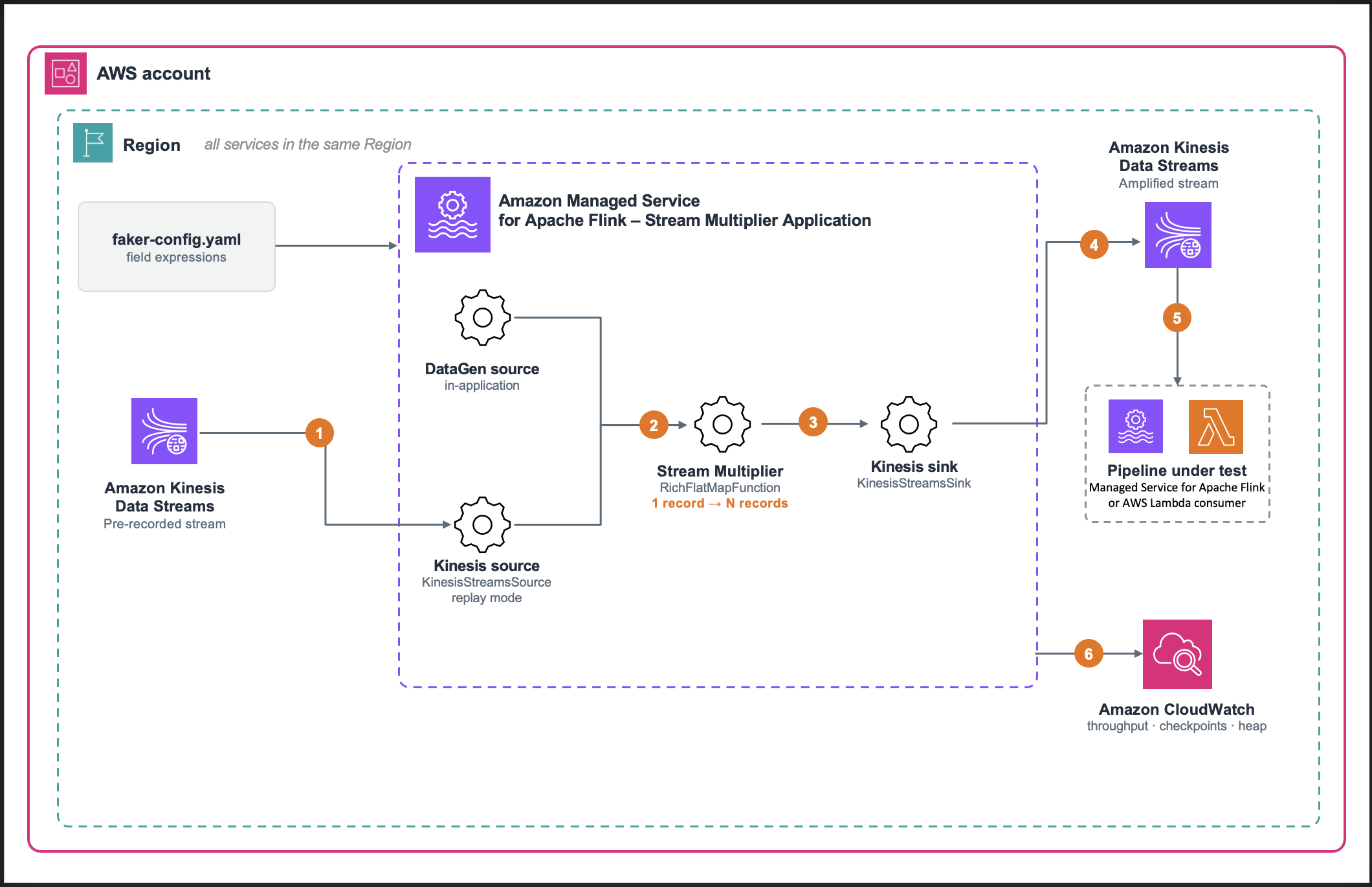
Architecture diagram. A pre-recorded Kinesis data stream, or an in-application DataGen source, feeds the stream multiplier on Managed Service for Apache Flink, which writes an amplified Kinesis stream to the pipeline under test.

Figure 1: Stream multiplier solution architecture

The solution uses three AWS services and one open source library:

  • Amazon Kinesis Data Streams holds the pre-recorded data stream on the source side, and carries the amplified stream to the pipeline under test on the sink side.
  • Amazon Managed Service for Apache Flink runs the multiplier, a RichFlatMapFunction that emits the original record plus N−1 variants.
  • Amazon CloudWatch collects the metrics that tell you whether the generator itself is healthy: throughput, backpressure, checkpoint duration, and heap.
  • DataFaker, an open source Java library for generating realistic synthetic values, produces the replacement values for mutated fields, driven by expressions you declare in faker-config.yaml rather than in code. It is declared as a build dependency and packaged into the application JAR, so there’s nothing to install separately.
  • The pattern is schema-agnostic: it operates on whichever fields you nominate as keys and whichever you nominate as mutable. In this sample, changing those fields is a configuration change. Adopting a different schema also requires updating the event model and the JSON serializers.

Prerequisites to deploy the stream multiplier

  • An AWS account with permissions to create Managed Service for Apache Flink applications, Kinesis data streams, Amazon Simple Storage Service (Amazon S3) buckets, and Amazon CloudWatch log groups.
  • A local build environment with Java Development Kit (JDK) 17 and sbt 1.9.9.
  • A source Kinesis data stream holding the pre-recorded data, and a sink stream sized for source throughput × multiplication factor.
  • An S3 bucket for the packaged application JAR.
  • AWS Command Line Interface (AWS CLI) version 2, configured.
  • An AWS Identity and Access Management (IAM) execution role with read access to the source stream and write access to the sink stream.

We tested the sample against these versions. The build.sbt file declares everything except the build tools, and sbt assembly bundles it into the JAR.

  • JDK : 17.
  • sbt : 1.9.9.
  • Scala : 2.12.20.
  • Apache Flink : 2.3.0.
  • Amazon Managed Service for Apache Flink runtime environment : FLINK-2_3.
  • aws-kinesisanalytics-runtime: 1.2.0.
  • Apache Flink Amazon Kinesis Streams connector : 6.0.1-2.0.
  • DataFaker : 2.7.0.
  • Jackson : 2.15.2.
  • Log4j : 2.24.3.

The Kinesis connector version is paired to the Flink version (6.0.1-2.0 targets Flink 2.x), and Flink 2.x requires Java 17 and uses the Java DataStream APIs, because the Scala DataStream APIs are no longer available.

A note on source data: This pattern doesn’t perform data masking, anonymization, or removal of personally identifiable information (PII). Fields that you don’t list in updatable.fields pass through unchanged. You are responsible for using only open data, or data that you sanitized, as the pre-recorded data stream. The walkthrough uses the public NYC taxi trip schema, which has the same shape as the AnyCompany Rides trip events.

Deploy the solution

The sample-datastream-multiplier repository includes an AWS CloudFormation template that creates the Kinesis data streams, the Managed Service for Apache Flink application, the IAM role, and the CloudWatch log group. It also creates an AWS Key Management Service (AWS KMS) key for log encryption and an AWS Lambda function that seeds the source stream with sample records.

  1. Build the uber-JAR with sbt assembly and upload it to your S3 bucket.
  2. Deploy infrastructure/cfn-template.yaml as a stack named data-stream-multiplier with aws cloudformation deploy, passing S3BucketArn and S3Key, and set MultipleFactor, KeyFields, and UpdatableFields as stack parameters.
  3. Start the application with aws kinesisanalyticsv2 start-application.
  4. Begin at a factor of 2x or 3x, confirm the output is correct, then raise the factor while monitoring CPU and backpressure.

The template encrypts both Kinesis data streams at rest with the AWS managed key (alias/aws/kinesis), and the CloudWatch log group with a customer managed AWS KMS key. To use your own key, pass EncryptionKmsKeyArn. If you reuse an existing source stream (CreateInputStream=false), you’re responsible for confirming that it has server-side encryption enabled. Amazon S3 encrypts the application JAR with SSE-S3 by default, and the AWS SDK uses TLS in transit.

Two ways to produce the stream

The multiplier reads from one of two sources, which you select with the source.type runtime property, and both feed the same multiplication operator. Amplification mode (source.type=kinesis) is the focus of this post. It replays a pre-recorded data stream, so fields you don’t replace keep the distributions of real traffic. Throughput is the source rate multiplied by multiple.factor. Pure synthetic mode (source.type=datagen) uses the Apache Flink DataGen connector to generate records in the application from faker-config.yaml, with no real data involved. It is useful for validating the pipeline end to end before you have a pre-recorded stream.

How it works

In amplification mode, the multiplier processes each incoming event in five steps:

  1. Read and deserialize the event from the source Kinesis data stream.
  2. Emit the original event unchanged.
  3. Compute a deterministic hash from the configured key fields combined with a per-iteration random seed.
  4. Generate synthetic values for the fields listed in updatable.fields, using that hash as the DataFaker seed and the expressions in faker-config.yaml. The key fields stay unchanged, so variants keep the same keys as the original.
  5. Serialize and write all records, original plus variants, to the sink stream.

Managed Service for Apache Flink application runtime properties drive the behavior, so the same artifact serves both modes regardless of schema:

Property Purpose
source.type kinesis for amplification mode, datagen for pure synthetic mode
multiple.factor Total records emitted per input record: 1 original plus N−1 variants
key.fields Business identifiers preserved across variants, and hashed to seed generation
updatable.fields Fields replaced with synthetic values in each variant
random.seeds One seed per multiplication iteration, so variants differ from each other
rate.limit.per.second Caps generated throughput in pure synthetic mode

The multiplication operator

The fan-out itself is deliberately small. A trait defines the contract, and flatMap is designed to emit the original followed by N−1 variants:

override def flatMap(value: IN, out: Collector[OUT]): Unit = {
  if (isValidEvent(value)) {
    emitOriginalEvent(value, out)
    for (i <- 1 until multiplier) {
      emitMultipliedEvent(value, out, i)
    }
  }
}

A multiplication factor of 3 produces three records: the original and two variants. The application validates the factor at startup and rejects values outside a range of 1 to 100. A mistyped factor can generate enough output to exhaust the sink’s shard capacity or the application’s heap. Bounding it in code helps prevent a configuration error from overwhelming the test environment.

Field generation with DataFaker

You define which fields become synthetic, and how, outside the code. Each entry pairs a DataFaker expression with a type:

trip_generation:
  from_location_name:
    expression: "#{options.option 'Manhattan - Times Square','Brooklyn - Williamsburg','JFK Airport','Harlem'}"
    expressionType: "string"

  distance:
    expression: "#{number.randomDouble '2','0','20'}"
    expressionType: "float"

  amount:
    expression: "#{number.randomDouble '2','5','150'}"
    expressionType: "float"

With key.fields=tripId and five updatable.fields, one input trip fans out into variants that share its identity but differ in the nominated fields. Three of the ten variants of a single trip, read back off the amplified stream during a 10x run:

{"tripId":8801,"timestamp":1789627092733,"fromLocationName":"Brooklyn - Williamsburg","toLocationName":"Manhattan - Central Park","distance":18.9,"amount":22.75,"category":"1"}
{"tripId":8801,"timestamp":1789627092733,"fromLocationName":"Bronx - Yankee Stadium","toLocationName":"Upper West Side","distance":0.1,"amount":69.85,"category":"2"}
{"tripId":8801,"timestamp":1789627092733,"fromLocationName":"Tribeca","toLocationName":"Tribeca","distance":4.29,"amount":128.88,"category":"3"}

tripId is identical on every variant because it is a key field, and timestamp because it appears in neither list and passes through untouched. The five updatable.fields differ in each. A consumer that groups by tripId still sees a coherent entity, because the key travels with every variant regardless of which shard carries it.
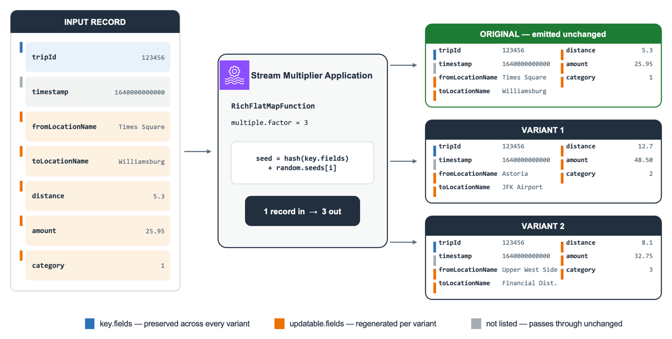
Diagram of one input record becoming three. tripId and timestamp stay the same in every output, while the multiplier regenerates location, distance, amount, and category per variant from the key-field hash plus random.seeds[i].

Figure 2: Inside the multiplier: the key field and untouched fields are identical on every variant, while the nominated fields are regenerated from a per-variant seed

The choice of
updatable.fields controls the trade-off between variant diversity and preservation of production distributions.

A repeatable, deterministic generator

If the generator produces different data on every run, a change in throughput or checkpoint duration between runs tells you nothing. The multiplier is therefore designed to be deterministic: the same pre-recorded data stream and the same configuration generate the same variant values on every run. After a failure and restore, replayed records regenerate the values they had before. The at-least-once Kinesis sink can still write some of them twice. Each variant’s values come from a seed built from the record’s key fields and a per-iteration seed from random.seeds, so variants are reproducible but still differ from one another. Because the generator is reseeded for every record, the values don’t depend on replay order after a restore or on which subtask processes the record. That holds only while every generated value comes from the seeded generator. Values such as wall-clock time or UUID.randomUUID() would break it.

What this looks like in practice

This section shows how the multiplier performed in our tests: first its throughput ceiling and resource use across factors, then how the sink’s shard count changes what you measure.

We ran a factor sweep on Managed Service for Apache Flink in the US West (Oregon) AWS Region (us-west-2). We deliberately over-provisioned the sink so that the multiplier itself was the only limit. The application ran at parallelism 2 with automatic scaling off, on 3 Kinesis Processing Units (KPUs): 2 for processing and 1 for orchestration. Records used the NYC taxi trip schema, averaging about 181 bytes, with key.fields=tripId, five updatable.fields, and one seed per variant. To hold the input rate constant, we used the pure synthetic (datagen) source with rate.limit.per.second and scaled the sink to 240 shards. Per-variant field generation, the compute-intensive path, runs the same code in both modes. Your results will vary with record size, schema, and configuration.

Throughput and capacity

Factor Input rec/s Output rec/s Output per processing KPU
5x ~25,600 ~128,000 ~64,000
10x ~14,300 ~143,000 ~71,500
15x ~11,300 ~169,000 ~84,500
20x ~8,600 ~171,000 ~85,500
25x ~7,040 ~176,000 ~88,000

Stability and resource utilization

Factor CPU % avg/max Backpressure Checkpoint duration Checkpoint size Heap % avg/max
5x 99 / 100 0 ~460 ms ~17 KB 31 / 63
10x 96 / 100 0 ~272 ms ~73 KB 34 / 65
15x 99.6 / 100 0 ~258 ms ~46 KB 35 / 59
20x 99.7 / 100 0 ~226 ms ~57 KB 38 / 66
25x 99.7 / 100 0 ~333 ms ~57 KB 36 / 63
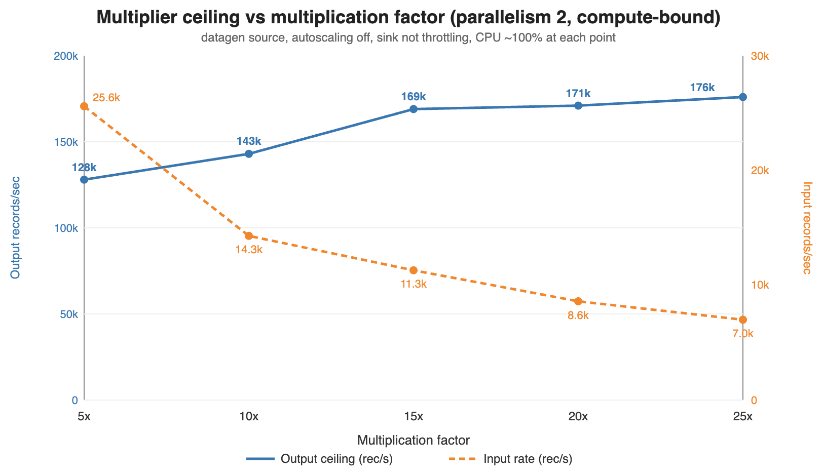
Line chart across factors 5x to 25x. Output rises from about 128,000 to 176,000 records per second and flattens, while the input rate the application consumes falls from about 25,600 to 7,040 records per second.

Figure 3: Output ceiling rises toward an asymptote as the factor increases, while the input rate the application can consume falls

Output throughput rises with the factor. Between 5x and 25x in our sweep, output climbed from approximately 128,000 to approximately 176,000 records per second while the input rate the application consumed fell from approximately 25,600 to approximately 7,040. Each input record carries a fixed cost to read and deserialize, and each output record carries the per-variant field generation cost. Raising the factor amortizes the fixed cost over more outputs, so output flattens near approximately 176,000 records per second.

CPU is the binding constraint, not memory and not state. CPU sits at 96–100 percent in every row, so in this configuration these plateaus are the multiplier’s ceiling. Heap stays in a narrow 31–38 percent average band with no upward trend. The job turns on Flink object reuse and reseeds one DataFaker instance per subtask instead of creating one per record. Checkpoints stay tiny, 17–73 KB completing in 226–460 ms, because the stateless flatMap has nothing to snapshot beyond source offsets.

For capacity planning, size from output per processing KPU: roughly 64,000 records per second at 5x, rising to approximately 88,000 at high factors.

Per-factor CloudWatch views show output rate in blue and sink throttling in red. The flat red line at zero indicates each plateau is compute-bound rather than sink-limited:
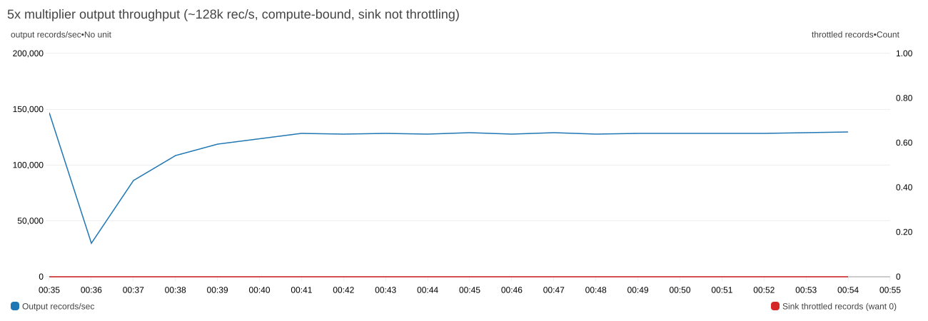
CloudWatch chart at 5x. After a brief dip at startup, output throughput holds steady near 128,000 records per second, while sink throttled records stay at zero throughout.

Figure 4: At 5x, output plateaus at ~128,000 records per second with zero sink throttling
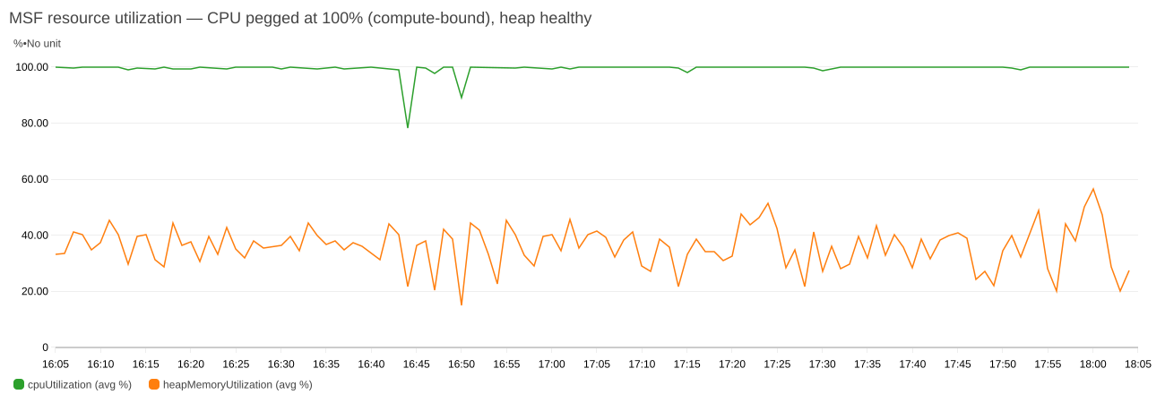
CloudWatch chart at 20x and 25x. CPU utilization stays near 100% for two hours apart from two brief dips, while heap memory utilization fluctuates between about 20% and 60%.

Figure 5: CPU pegged near 100% while heap stays comfortable. This is the signature of a compute-bound plateau

Your sink decides your throughput, not the multiplier

That ceiling is only reachable if the sink can absorb it. Holding the factor at 10x and changing nothing but the sink’s shard count shows where the real limit usually sits:

Sink shards Sink capacity rec/s Observed output rec/s Throttling CPU % Limited by
20 20,000 ~20,505 heavy ~16 sink
60 60,000 ~62,000–70,000 heavy ~48 sink
120 120,000 ~122,000–123,000 mild ~86 sink (marginal)
180 180,000 ~143,000 none ~96 compute (ceiling)

At 20 shards the application ran at 14 percent of its capability with CPU at 16 percent, waiting on the sink. Only at 180 shards does throttling disappear and CPU saturate, so you are measuring the multiplier rather than your Kinesis provisioning.

A shard accepts 1,000 records or 1 MB per second on writes, whichever limit you reach first. For records under about 1 KB, like the approximately 181-byte trip events here, the record limit applies first. The sink needs roughly target output rate ÷ 1,000 shards before any factor comparison is meaningful. For larger records, size by bytes: one shard per MBps of target output. Under-provision it and every factor reports the same throughput: the shard limit.

The async KinesisStreamsSink re-queues and retries throttled records. Across our sweep, transient per-attempt failures stayed at 73 or fewer in a window against tens of millions of records, and we observed no permanent loss. Write latency held at approximately 40–54 ms average with occasional approximately 1.1 s spikes.

Shard load also stays even as the factor rises, because the partition key comes from the record’s hash rather than the multiplication factor. In our 25x run across 240 open shards, every shard carried between 671 and 678 records per second, within about 0.5 percent of the approximately 675 average.

Validating a run

Before you trust the load test, confirm that the multiplier is doing what you expect:

  1. Measure throughput on the Kinesis side, not the application side. Flink chains the source, the multiplier, and the sink into a single operator. As a result, the application-level numRecordsInPerSecond and numRecordsOutPerSecond don’t cleanly separate input from output. Use GetRecords.Records on the source stream and IncomingRecords on the sink stream. Their ratio is the true fan-out and should equal your multiplication factor. In our 10x amplification run, it measured 2,056 records per second in against 20,505 out, a ratio of 9.97.
  2. Key preservation. Sample the sink stream and confirm that variants share key-field values and that fields outside both lists are unchanged.

Troubleshooting

If the amplified stream isn’t what you expect, check these first:

  • All variants of a record are identical. random.seeds has fewer entries than the multiplication factor requires.
  • Output rate is below factor × input rate. Check WriteProvisionedThroughputExceeded on the sink and backPressuredTimeMsPerSecond on the operator, and provision at least target output rate ÷ 1,000 sink shards for records under about 1 KB.
  • The source falls behind. Watch millisBehindLatest on the application or GetRecords.IteratorAgeMilliseconds on the source stream. If the lag climbs during a live run, add source shards or use Enhanced Fan-Out and watch SubscribeToShardEvent.MillisBehindLatest instead.
  • The application crash-loops after switching source.type. Switching modes changes the job graph, so restoring the previous snapshot fails with a KinesisShardSplitSerializer EOFException. Start the application with SKIP_RESTORE_FROM_SNAPSHOT. The multiplier is stateless, so there is no application state to restore. Property changes, including source.type, take effect only after an application update.

Performance considerations and limitations

The multiplier inherits the timing of the pre-recorded data rather than synthesizing it. Amplification multiplies volume and keeps the sample’s timing shape, so bursts in the pre-recorded data carry through at higher amplitude. Injecting bursts that are not in the sample, spreading variants over an interval rather than emitting them together, and simulating late arrival all need extra logic. The sample uses WatermarkStrategy.noWatermarks() because the multiplier has no event-time operators. Flink also doesn’t write watermarks into Kinesis records, so the watermark setting in the multiplier has no effect on the pipeline under test. Each variant keeps the original timestamp in its payload. The pipeline under test assigns its own watermarks from that field, as it does in production.

Generated fields are independent of each other. Each entry in faker-config.yaml is evaluated on its own, so in the trip example, distance is drawn from 0–20 and amount from 5–150 with no relationship between them. A 0.5-mile trip can be assigned a $150 fare. Ordering is preserved within a partition but not across partitions, so if the pipeline under test depends on global ordering, the amplified stream won’t provide it.

The sample assumes that the source and sink streams are in the same AWS account. For a stream in another account, grant the application’s execution role access with a resource-based policy on that stream. The sample also reads and writes JSON. Because the multiplier works on deserialized objects, supporting Apache Avro or Protocol Buffers means replacing JsonDeserializationSchema and JsonSerializationSchema. The multiplication logic is unchanged.

Cost considerations

You pay for Kinesis shard-hours, PUT payload units, and extended retention, and for Managed Service for Apache Flink KPU-hours and running application storage. Amazon CloudWatch Logs and AWS KMS add smaller charges. The following estimates are approximate and use on-demand prices in US West (Oregon) as of October 2026. Prices vary by AWS Region and change over time, so check Amazon Kinesis Data Streams pricing, Amazon Managed Service for Apache Flink pricing, or the AWS Pricing Calculator for your Region.

Default deployment. The template runs three shards with seven-day retention and 3 KPUs, two for processing and one for orchestration. That comes to about $0.45 per hour, or about $11 per day if you leave it running, plus PUT payload units for the records you write. Automatic scaling is on by default and can add KPUs under load.

The 25x run in this post. Two hours at 25x, with 240 sink shards and about 176,000 records per second, uses about 1.3 billion PUT payload units ($17.75), 480 sink shard-hours ($7.20), and 6 KPU-hours ($0.66), for about $26. Seven-day retention adds about $9.60, for about $35. Lower factors write fewer records and cost less.

To keep costs down, set StreamRetentionHours to 24 unless you plan to replay the amplified stream. Size the sink to your target output rate, keep test windows short, and follow the clean-up steps as soon as you finish.

Clean up

To avoid ongoing charges, stop the application, wait until it reports READY, then delete the stack:

aws kinesisanalyticsv2 stop-application --application-name DataStreamMultiplier --force
aws cloudformation delete-stack --stack-name data-stream-multiplier

Deleting the stack removes the Kinesis data streams, the application, the IAM role, the producer Lambda function, and the log group. If the stack created the AWS KMS key, AWS CloudFormation schedules it for deletion after a 30-day waiting period. Delete the JAR from your S3 bucket separately.

Conclusion

Validating a streaming pipeline at production scale requires a data source that delivers both realistic data and sustained volume. With the stream multiplier pattern, real distributions come from the pre-recorded capture, and you control volume through a single parameter, multiple.factor, rather than through storage. To get started, clone the sample-datastream-multiplier repository and follow the steps in Deploy the solution, starting at a factor of 2x or 3x. For more on building and running applications on the service, see the Amazon Managed Service for Apache Flink Developer Guide.


About the authors

Siva Mahamkali

Siva Mahamkali

Siva is a Senior Streaming Data Consultant at Amazon Web Services (AWS). He specializes in real-time data streaming, stream processing with Apache Flink, and data platform modernization, and applies generative AI and agentic AI to help organizations build streaming solutions on AWS that scale reliably to production volumes.

Mitali Sheth

Mitali Sheth

Mitali is a Streaming Data Engineer at AWS Professional Services, where she helps enterprise customers build real-time analytics solutions and event-driven architectures. She specializes in Amazon Managed Streaming for Apache Kafka, Amazon Managed Service for Apache Flink, AWS Glue, and AWS Lake Formation. She holds an M.S. in Computer Science from the University of Florida.

Nagesh Honnalli

Nagesh Honnalli

Nagesh is a Principal Engineer at Amazon Web Services (AWS) with 15 years of experience building distributed systems. He leads the technical strategy and execution for Amazon Managed Service for Apache Flink, Amazon Managed Streaming for Apache Kafka (Amazon MSK), and Amazon MSK Connect. He has helped build and launch several AWS streaming services, including Amazon Managed Service for Apache Flink, Amazon Kinesis Data Analytics for SQL, and Amazon Data Firehose. When he isn’t working, he enjoys biking, cooking, and his favorite job: being dad to his 7-year-old daughter.

Ryan Braley

Ryan Braley

Ryan is an Engineering Leader at Amazon Web Services (AWS). He leads engineering teams, guiding them in designing and implementing scalable, high-performance data and AI platforms for AWS customers. With expertise spanning distributed systems, real-time and batch data architectures, and cloud-native infrastructure, he drives technical strategy and engineering excellence across teams. He is passionate about raising the bar on engineering practices and solving large-scale problems at the intersection of data and business impact.

Satish Gutta

Satish Gutta

Satish is a Delivery Consultant at Amazon Web Services. He specializes in distributed data processing using Apache Flink and Apache Spark, with deep expertise in streaming architectures. He partners with customers across diverse industries to design and deliver scalable real-time and batch data solutions, helping them turn complex data challenges into reliable, production-ready pipelines.

[$] Synaptics patent claims stop work on DisplayLink drivers

Post Syndicated from jzb original https://lwn.net/Articles/1102549/

Mike Lothian owns a docking station (or dock) that uses a DisplayLink chipset
that had, at least in his opinion, subpar performance on Linux. He
decided to try improving the Linux driver, with LLM assistance, but ran into one
problem that he could not solve—so he asked for help, hoping that
Synaptics’s developers would lend a hand. (DisplayLink was acquired by
Synaptics
in 2022.) Rather than help him in improving the
driver, however, the Synaptics legal team responded with patent infringement
claims, a demand
that he cease unauthorized implementation of DisplayLink technology, and threats
of expensive legal penalties. For now, it appears that Linux users of the
company’s docks will have to continue to live without feature parity with other
platforms.

Critical vulnerabilities in N-able N-central prompt hosted shutdown

Post Syndicated from Rapid7 original https://www.rapid7.com/blog/post/etr-critical-vulnerabilities-in-n-able-n-central-prompt-hosted-shutdown

Overview

On November 9, 2026, N-able announced that it was responding to the public disclosure of critical vulnerabilities affecting N-central, its remote monitoring and management (RMM) platform.

In a public disclosure titled Able2Shell, an independent researcher has published details and proof-of-concept (PoC) code covering 33 issues. According to the disclosure, the issues include unauthenticated remote code execution (RCE), privilege escalation to root, credential disclosure, and unauthorized account creation. One unauthenticated chain combines XML external entity (XXE) and session-handling weaknesses to execute code as the nable service account. Other demonstrated chains involve an administrator viewing malicious patch metadata or use ProductAdmin credentials. Rapid7 Intelligence is currently triaging the newly published details.

Before the hotfix release on November 10, N-able reported scanning activity associated with the published PoC code and said it had no evidence that any customer environment had been successfully exploited. The vendor advised keeping N-central deployments offline while it developed and validated a hotfix. Hosted N-central classic environments were offline, according to the same notice. That notice did not yet include CVE identifiers or CVSS scores.

N-central is used by managed service providers (MSPs) and enterprise IT teams to administer endpoints and infrastructure. Compromise of an RMM server can put downstream managed environments at risk. N-central has previously been targeted through separate vulnerabilities, including an authentication bypass covered by Rapid7 in August 2026. Given the platform’s administrative reach and the availability of public exploit code, Rapid7 recommends treating the current disclosure as an emergency.

Update #1: On November 10, 2026, N-able released N-central 2026.4 Hotfix 2 (build 2026.4.1.26), addressing seven CVEs. The vendor plans a follow-up hotfix with further security updates. On November 11, N-able confirmed that hosted N-central servers across all regions had been successfully upgraded.

Mitigation guidance

Rapid7 strongly recommends that organizations operating on-premises N-central servers upgrade to N-central 2026.4 Hotfix 2 (build 2026.4.1.26) on an emergency basis outside of normal patching cycles, and keep servers offline until successfully upgraded. Hosted servers are upgraded by N-able.

Customers in both hosted and on-premises environments must also upgrade their Agents and Probes. To maintain communication, upgrade Agents first, then Probes, following the vendor’s compatibility guidance for the Patch Management Engine (PME).

  • Affected versions: The researcher reports testing N-central Appliance 2026.4.0.31. N-able’s current notice does not specify the full affected-version range.

  • Fixed versions: N-central 2026.4 Hotfix 2 (build 2026.4.1.26) addresses the seven CVEs listed below.

According to N-able’s release notes, the hotfix addresses:

CVE

Description

CVE-2026-125883

Multiple XXE vulnerabilities

CVE-2026-125878

Multiple OGNL injection vulnerabilities

CVE-2026-125879

Local privilege escalation to root through nable-writable syslog-ng configuration

CVE-2026-125880

Stored XSS through MMS3 patch metadata in an administrator context

CVE-2026-125881

Schema-hint SSRF through service-import schema validation

CVE-2026-125882

RCE through file-repository upload path traversal; credited to Nate Fair, Sprocket Security

CVE-2026-91000

Local privilege escalation through insecure IPC channels

Further security updates are planned in a follow-up hotfix. Organizations should monitor the vendor’s guidance and apply subsequent fixes as they become available.

Rapid7 also recommends reviewing N-central servers and downstream managed systems for signs of compromise and engaging incident responders if suspicious activity is identified.

For the latest mitigation guidance, please refer to N-able’s security incident notice.

Rapid7 customers

Exposure Command, Vulnerability Management, and Nexpose

Exposure Command, Vulnerability Management, and Nexpose customers can identify N-able N-central “potential” vulnerabilities based on presence of software with remote unauthenticated checks with the release on November 11th, 2026. Note that potential check type must be enabled in the scan template before scanning.

Unauthenticated checks that validate vulnerable versions are in development.

Intelligence Hub

Customers leveraging Rapid7’s Intelligence Hub can access Suricata detection rules for CVE-2026-125883, CVE-2026-125878, CVE-2026-125879, CVE-2026-125880, CVE-2026-125881, and CVE-2026-125882.

Updates

  • November 10, 2026: Initial publication.

  • November 11, 2026: Added hotfix availability, seven CVE identifiers, hosted upgrade confirmation, and updated remediation guidance. Noted the planned follow-up hotfix.
  • November 11, 2026: Added availability of Suricata detection rules within Intelligence Hub.
  • November 11, 2026: Added Exposure Command, Vulnerability Management, and Nexpose subsection under the Rapid7 customers section.

Five Signs Your MDR is All Alert, No Action

Post Syndicated from Rapid7 original https://www.rapid7.com/blog/post/five-signs-your-mdr-is-all-alert-no-action

Your managed detection and response (MDR) provider flags suspicious activity, and your analyst spends the next hour finding the account, checking logs, and deciding whether anything needs to happen. By the time the investigation is underway, the alert feels less like help and more like a task assignment. 

MDR should bring your team capacity and expertise when it needs them. If the service keeps handing the hardest work back to your analysts, these five signs can help you work out where the arrangement is falling short.

1. Every alert arrives with homework

If your analysts are still sorting through the same recurring false positives, the extra coverage may be creating more work than it removes. Even an alert worth investigating is only so useful when your team has to gather the basic context before it can make a decision. Take a few recent alerts and look at what your provider had already checked when it contacted you. You should be able to see how it separated routine activity from a credible threat, and what it did to stop familiar noise from coming back.

2. It spots the fire, but cannot see the fuel

A suspicious login involving an account with broad access deserves a different response from the same activity on a tightly restricted account. The systems within reach, their importance to the business, and any known weaknesses all help determine what needs attention first. When your MDR leaves your team to assemble that picture during an investigation, valuable time goes into finding context that could have informed the response from the start. Find out how your provider uses information about assets, identities, vulnerabilities, and current threats, including what it can help you address before an incident occurs.

3. Your team gets incident updates, but few useful lessons

When a provider contains a threat and closes the case, your team should come away with more than a record of what happened. Consider the last significant investigation: did it lead to a clearer detection, a stronger response plan, or a better understanding of how an attacker moved through your environment? If similar activity appears three months later and your analysts have to work through the same questions, the service has missed a chance to make them better prepared. Expertise is most useful when your team can apply some of it next time.

4. Your response support has a spending limit

If an incident is still developing when your included response hours run out, continued specialist support may require another purchasing decision. Limits on hours, incident scope, or responder involvement can turn an agreed service into an unplanned budget request under pressure.

Ask what happens when an investigation expands across systems or continues longer than expected. Establish whether incident response is unlimited, which activities that includes, how long specialists stay involved, and what could trigger additional charges. When business operations and leadership confidence are already at stake, uncertainty about continued support adds financial and operational pressure at the point you need a clear path forward.

5. Your provider’s reports prove it was busy

A monthly report might show hundreds of alerts reviewed and dozens of investigations opened. That gives you a sense of volume, though it says little about what the provider found or did. Choose a closed investigation and follow it from the initial signal through to the outcome: what evidence was considered, what was ruled out, what action was taken, and when did your team become involved? If you need several calls to piece together that story, the charts are doing a better job of showing activity than the service is of showing its work.

If several of these signs feel familiar, bring a few real alerts and investigations to your next service review. Ask your provider to show what it investigated, which actions it took, and what improved afterward. The answers will give you a clearer view of the work your MDR is taking on and the work that still lands with your team.

For more questions to use when reviewing your service, explore the MDR buyer’s guide.

Security updates for Tuesday

Post Syndicated from jzb original https://lwn.net/Articles/1106522/

Security updates have been issued by AlmaLinux (curl, dpdk, glibc, kernel, nodejs-nodemon, nodejs22, nodejs24, nodejs:18, nodejs:22, patch, qt5, qt5-qtdeclarative, ruby, ruby4.0, ruby:3.3, ruby:4.0, squid:4, tomcat, util-linux, and webkit2gtk3), Debian (symfony and tomcat10), Fedora (bind, dnf5, kernel, kernel-headers, libmodulemd, maturin, perl-CGI, perl-Net-IDN-Encode, perl-Starlet, python-jiter, python-pydantic-core, python-pysequoia, python3-docs, python3.14, python3.15, ruff, rust-afterburn, rust-astral_async_zip, rust-clearscreen, rust-jiter, rust-lzma-rust2, rust-mailparse, rust-pyo3-introspection, rust-python-pkginfo, rust-serde_json, rust-testresult, rust-zip, selenium-manager, ty, and uutils-coreutils), Mageia (glibc, packages, php-smarty, python-aiohttp, and thunderbird), Oracle (curl, firefox, gdb, glibc, kernel, oVirt 4.5 ovirt-engine-wildfly, perl-YAML:1.24, and tesseract), Slackware (krb5), SUSE (ansible-core, apr-util, aspell, buildpacks-cli, dpdk22, firefox, git-bug, glib2, google-cloud-sap-agent, haproxy, jsoup, kernel, krb5, libjxl, librsvg, libruby4_0-4_0, libunbound8, libXtst, nodejs24, nvidia-open-driver-G07-signed, PackageKit, perl-XS-Parse-Keyword, poppler, python, python-Brotli, rsyslog, tekton-cli, tomcat, tomcat10, tomcat11, trivy, udisks2, xen, zchunk, and zk), and Ubuntu (apache2, ca-certificates, fetchmail, freerdp3, kernel, libgphoto2, libheif, libnfs, libsoup3, linux, linux-aws, linux-aws-5.15, linux-aws-fips, linux-azure, linux-azure-5.15, linux-azure-fde-5.15, linux-azure-fips, linux-gcp, linux-gcp-5.15, linux-gcp-fips, linux-gke, linux-gkeop, linux-hwe-5.15, linux-ibm, linux-ibm-5.15, linux-intel-iot-realtime, linux-intel-iotg, linux-intel-iotg-5.15, linux-kvm, linux-lowlatency, linux-lowlatency-hwe-5.15, linux-nvidia, linux-nvidia-tegra, linux-nvidia-tegra-5.15, linux-oracle, linux-oracle-5.15, linux-realtime, linux, linux-aws, linux-aws-fips, linux-aws-hwe, linux-azure, linux-azure-4.15, linux-azure-fips, linux-fips, linux-gcp, linux-gcp-4.15, linux-gcp-fips, linux-hwe, linux-kvm, linux-oracle, linux, linux-aws, linux-aws-fips, linux-azure, linux-azure-5.4, linux-azure-fips, linux-bluefield, linux-fips, linux-gcp, linux-gcp-5.4, linux-gcp-fips, linux-hwe-5.4, linux-ibm, linux-ibm-5.4, linux-iot, linux-kvm, linux-oracle, linux-oracle-5.4, linux-xilinx-zynqmp, linux, linux-aws, linux-azure, linux-azure-fips, linux-gcp, linux-gke, linux-ibm, linux-lowlatency, linux-oracle, linux-vmware, linux, linux-aws, linux-gcp, linux-ibm, linux-oem-7.0, linux-oracle, linux, linux-aws, linux-kvm, linux-lts-xenial, linux-aws, linux-aws-5.4, linux-raspi, linux-raspi-5.4, linux-aws-6.8, linux-gcp-6.8, linux-ibm-6.8, linux-lowlatency-hwe-6.8, linux-nvidia, linux-realtime-6.8, linux-aws-7.0, linux-azure-fde, linux-azure-fde-7.0, linux-gcp-7.0, linux-gke, linux-oracle-7.0, linux-realtime, linux-aws-fips, linux-gcp-fips, linux-gkeop, linux-realtime, linux-azure, linux-azure-6.8, linux-azure-fde-6.8, linux-azure-fde, linux-oracle-6.8, linux-raspi, linux-raspi-realtime, linux-raspi, openjdk-17, openjdk-21, openjdk-25, openjdk-27, openjdk-8, openjdk-lts, perl, and pyasn1).

New OpenSSH Vulnerability

Post Syndicated from Bruce Schneier original https://www.schneier.com/blog/archives/2026/11/new-openssh-vulnerability.html

It’s a bad one, and it’s been in the code for a decade:

A newly disclosed flaw involving OpenSSH and musl, dubbed “*sshole,” allows attackers to log in to certain Alpine Linux and other musl-based Linux accounts configured to block password authentication simply by entering an oversized password.

“Oversized” means longer than 256 bytes. Details.

Slashdot thread. And another news article.

Automate ETL pipeline creation with Amazon Bedrock AgentCore and AWS Glue

Post Syndicated from Mike Brouwers original https://aws.amazon.com/blogs/big-data/automate-etl-pipeline-creation-with-amazon-bedrock-agentcore-and-aws-glue/

If you run data pipelines, you know how much work they can take to set up, sometimes only to break without you realizing. That doesn’t even include data from sources too small to justify a project of their own, such as instrument exports, partner CSV files, and database tables. Each one can take an engineer days to map, code, test, and provision, and the work needs to be repeated when the schema changes.

Agentic Data Ingestion, the solution referenced in this post, automates that work with agentic AI. You point it at a file or a database table, and foundation models (FMs) propose the field mapping and write the transformation code. The agent tests that code on Apache Spark before it deploys the code as an AWS Glue job, and you approve or reject the result at the mapping or code testing step. In our test deployment, a run at sample scale costs about USD $0.10–0.25, and the idle deployment about USD $15–20 a month. For more information, see Cost to run the solution.

To see it in action before you deploy, try the interactive demo.

In this solution, the FMs run on Amazon Bedrock, which is a fully managed service that provides foundation models, and the agents, built with the open-source Strands Agents SDK, run on Amazon Bedrock AgentCore, which hosts and operates AI agents. AWS Step Functions, which provides serverless workflow orchestration, manages each run, and AWS Glue, which provides serverless data integration capabilities, runs the generated jobs. You deploy the whole solution with the AWS Cloud Development Kit (AWS CDK). Before you begin, review the Prerequisites.

Solution overview

The following diagram shows the architecture.

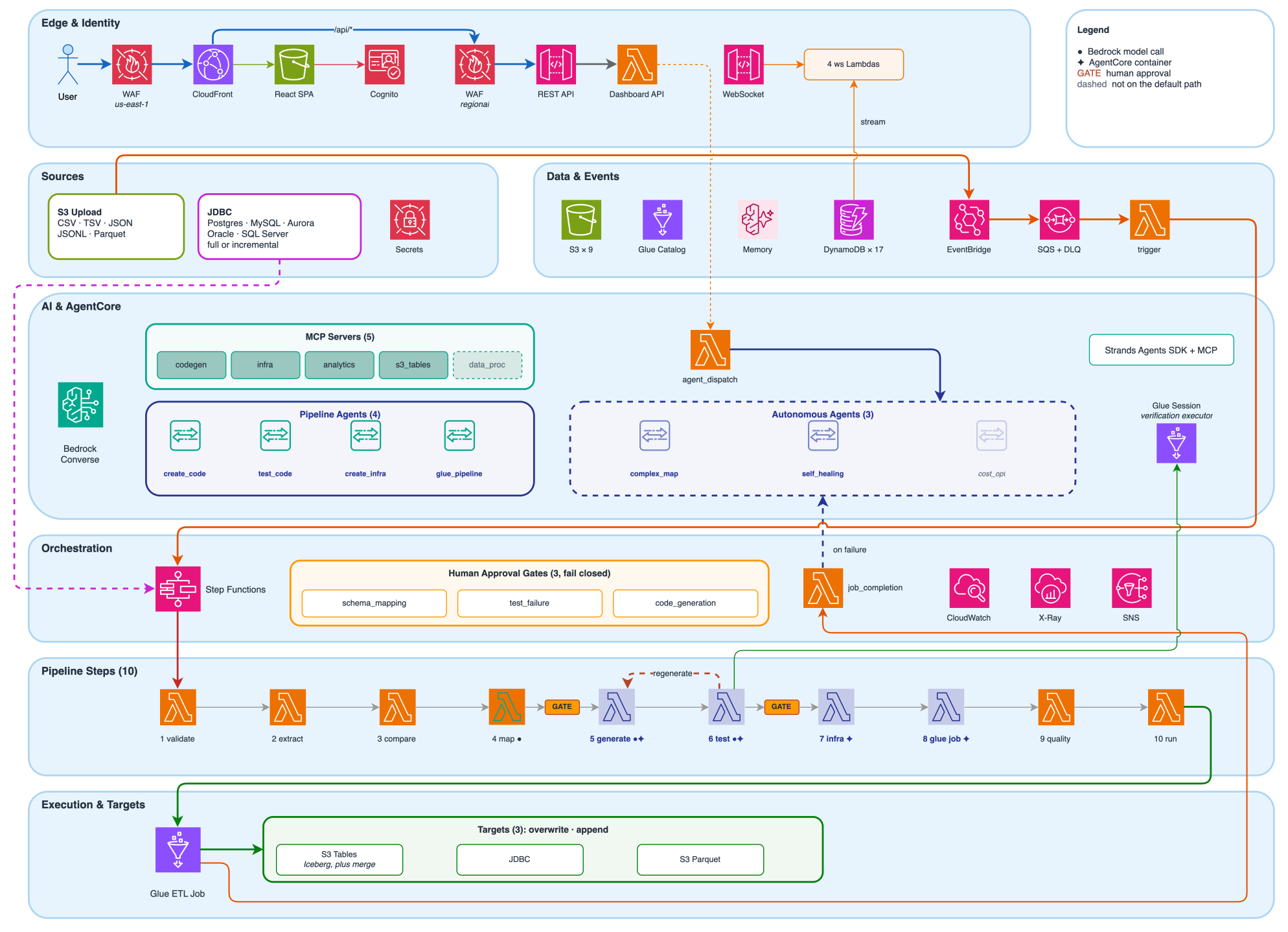
Agentic Data Ingestion architecture, showing six layers: edge and identity, sources, data and events, AI and AgentCore, orchestration, and execution and targets

Figure 1: Solution architecture, from sign-in and the data sources through the agents and Step Functions orchestration to the AWS Glue job and its targets

The solution includes a React dashboard that shows each run’s progress and the approval gates. An upload to the source Amazon Simple Storage Service (Amazon S3) bucket travels through Amazon EventBridge and Amazon Simple Queue Service (Amazon SQS), an event bus and a message queue, to a trigger function on AWS Lambda, which provides serverless compute capabilities, starts a 10-step Step Functions workflow:

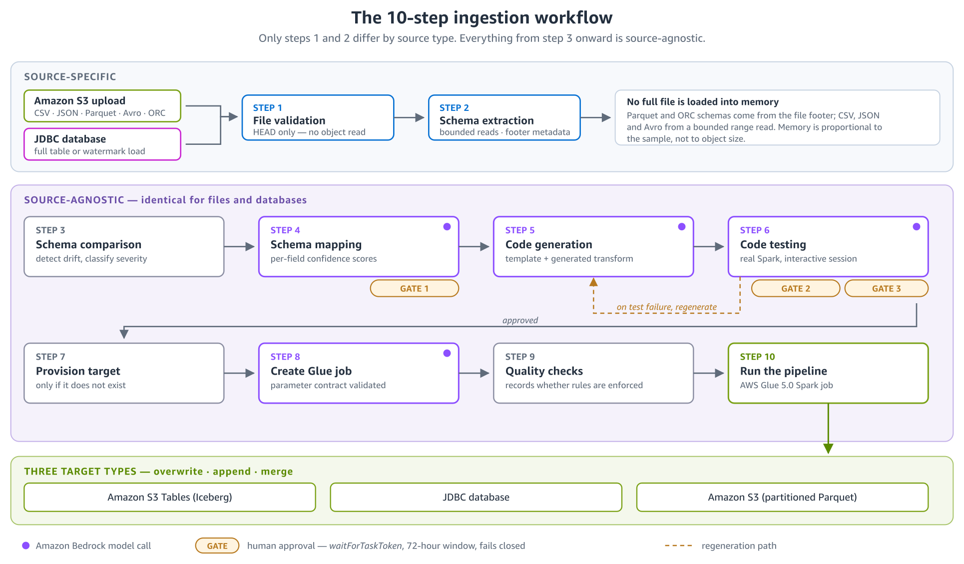
  1. File validation – Check format and size from object metadata.
  2. Schema extraction – Infer field names and types.
  3. Schema comparison – Detect drift against the target schema.
  4. Schema mapping – An FM maps source to target fields with confidence scores. (Approval gate).
  5. Code generation – Generate the PySpark transform and data quality rules.
  6. Code testing – Run the transform on Spark and check its output. (Approval gate, plus a forced review if tests keep failing).
  7. Infrastructure provisioning – Create the target if it doesn’t exist.
  8. AWS Glue job creation – Create the job with a validated configuration.
  9. Quality checks – Record which data quality rules the job will enforce.
  10. Run pipeline – Run the AWS Glue job.

The data quality rules, for AWS Glue Data Quality, a capability of AWS Glue, come from the approved mappings and run inside the job, which quarantines failing rows before it writes. They’re on by default for file uploads into Amazon S3 Tables, a capability of Amazon S3, which stores Apache Iceberg tables, and optional for the other targets.

The 10-step workflow. Steps 1 and 2 are source-specific. Steps 3 through 10 are source-agnostic. Approval gates sit after step 4 and after step 6, and a failing test returns to step 5 for regeneration

Figure 2: The 10-step workflow. Steps 1 and 2 depend on the source type, approval gates follow steps 4 and 6, a failing test returns to step 5, and the job writes to one of three target types

Supported sources and targets

Source Details
Amazon S3 upload CSV (including TSV and pipe-delimited), JSON, Parquet, Avro, ORC, and Excel (.xlsx, one worksheet per run). Each file starts its own run.
JDBC database PostgreSQL, Amazon Aurora, MySQL, MariaDB, Oracle, or SQL Server through the AWS Glue Java Database Connectivity (JDBC) connector, on demand or on a schedule. Incremental loads read only rows newer than the last run, keyed on a timestamp or numeric watermark column.
Target Details
Amazon S3 Tables Apache Iceberg tables (append, overwrite, or merge), queryable from Amazon Athena, Amazon EMR, and Amazon Redshift after you enable the analytics integration.
JDBC database Relational databases, including Amazon Relational Database Service (Amazon RDS). Credentials come from AWS Secrets Manager at run time.
Amazon S3 (Parquet) Partitioned Parquet in a bucket you own.

How we made generated code reviewable and repeatable

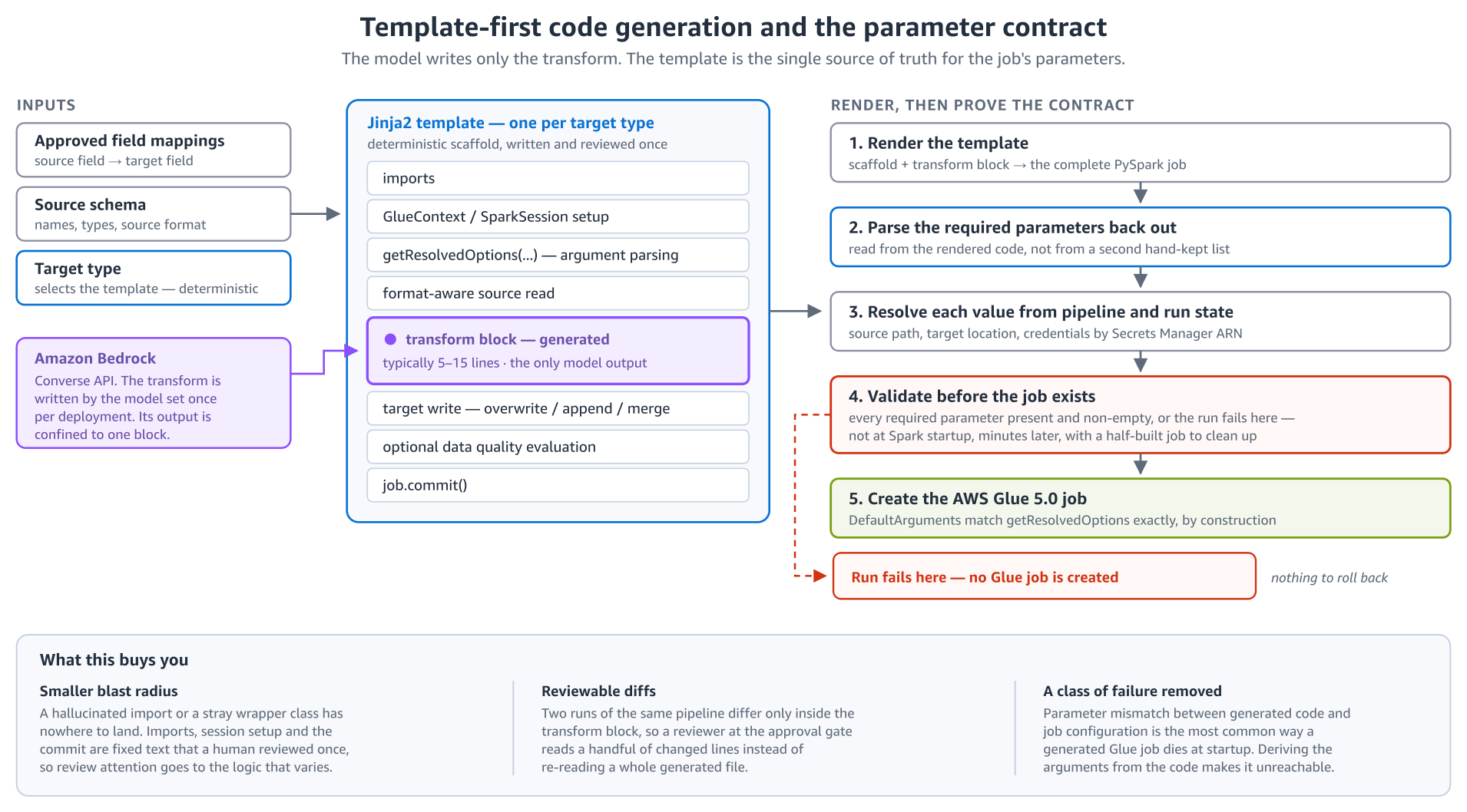
In our very first attempt, we asked the model to create the whole AWS Glue script, more than 500 lines on each run. Reviewing that each time wasn’t sustainable. It failed for random reasons, and because the model is non-deterministic, the next run could fail somewhere new no matter how much we optimized the prompt. To solve this, we made the job as deterministic as we could. A human-written/reviewed Jinja2 template for each target type now supplies the scaffold, and the FM writes only the transformation block, typically 5–15 lines for these samples, which is checked against an allowlist of permitted constructs before the job is created.

In our next iteration, these jobs failed inconsistently with GlueArgumentError because different parts of the code used different names for the same job arguments. We made the code itself consistent, but not how the arguments were named. The solution parses the parameters that the rendered code reads with getResolvedOptions, resolves a value for each, and refuses to create the job if one is missing.

Template-first code generation. Inputs feed a Jinja2 template whose transform block is model-generated. The rendered job is then parsed for required parameters, each value resolved, and all parameters validated before the AWS Glue job is created

Figure 3: Template-first code generation. The model writes only the transform block, and the job’s parameters are validated before the job is created

When we first started testing, we translated the PySpark into pandas, which we thought would simplify testing. But this approach couldn’t express everything PySpark can. It failed inconsistently and could never guarantee the script would work, which defeats the purpose of testing. So now the transform runs in an AWS Glue interactive session on the same Spark version as the job, against a 100-row sample of the source file. Its output is checked for record counts, nulls, and schema compliance. Database sources are tested on rows generated from the schema instead, because the test session in the workflow has no access to your databases.

Human approval gates

To review the results before continuing while you build trust in the pipeline, two gates pause a normal run and wait for approval, one after schema mapping and one after the code passes its tests. A mapping skips review only when each field pair is high-confidence and corroborated by a name match, and a reused mapping goes to review by default.

The gates fail closed, so if the workflow can’t tell whether a step needs review, it waits for a person. A run left waiting at a gate for 72 hours fails, and approvals and rejections are recorded with the reviewer’s identity. Two agents can help along the way. When mapping confidence is low, a complex-mapping agent adds sample values and specific questions to the mapping review. When an AWS Glue job fails, a self-healing agent starts one new run, which regenerates the code after a schema or type error or uses a larger worker after an out-of-memory error. It skips the retry when a second run could duplicate data the failed job already wrote, or when a retry can’t fix the error, such as a permissions problem. The run then stays failed, with the agent’s diagnosis on its detail page. For the full rules, see Approval Gates and the agents guide.

Customer perspective: Montai Therapeutics

Montai Therapeutics applies the same pattern to scientific data. Rather than hand-writing a parser for each new assay format, the team embedded an agent that generates the parser into the ingestion application they already had.

“We have implemented agentic parser generation to ingest semi-structured or variably formatted scientific data into our schema-controlled system of record. Embedding the parser function generation agent into our existing ingestion app has brought lead time to onboard and deploy new assays and protocols to near zero (5 to 10 minutes for parser generation and output checking on an agent runtime), where before there could be days to weeks of developer time spent scripting bespoke parsing functions that may only be used a few times.

The biggest business impact has been the proportion of experimental data that now lands in our data lake rather than in people’s inboxes, which will funnel into improving our drug specificity and efficacy predictive models. Time spent by scientists troubleshooting data formatting issues is now relegated to solving the scientific problems at the core of our business strategy.”

— Kevin Klicki, Senior Engineer – Bioinformatics, Montai Therapeutics

Security considerations

Generated code runs in an isolated test session under a read-only role before an AWS Glue job exists. The solution creates dedicated AWS Identity and Access Management (IAM) roles for pipeline jobs, scoped to that pipeline and bounded by a permissions boundary, with separate roles for agent runtimes. Data is encrypted at rest and in transit, and JDBC credentials are referenced only by their Secrets Manager Amazon Resource Name (ARN), so they don’t appear in job arguments.

You sign in through Amazon Cognito, with multi-factor authentication (MFA) required by default. The dashboard is served through Amazon CloudFront behind an AWS WAF web access control list (web ACL) with managed rules and a rate limit. A second web ACL admits only API requests that come through CloudFront. By default, signed-in users have full dashboard access. The solution doesn’t include identity federation or role-based access, which the README’s Hardening for real data section lists as next steps for production.

Cost to run the solution

We measured these figures on our test deployment in the US West (Oregon) AWS Region (us-west-2) with the repository’s sample files, which have seven or eight columns, and priced the usage at public list prices.

Idle, the solution costs about USD $15–20 per month. About USD $14 is the two AWS WAF web ACLs and their rules, up to USD $5 is Amazon CloudWatch monitoring, depending on your free tier, and storage and one secret add about USD 1. Everything else bills per use.

A run at sample scale costs about USD $0.10–0.25:

Component Grows with Per run, measured Basis
Amazon Bedrock, Claude Sonnet 4.6 Number of fields and model calls USD $0.05–0.14 About 10,500 tokens over three model calls on a clean run, up to 32,000 with regeneration, at USD $3.30 and USD $16.50 per million input and output tokens (us. inference profile)
AWS Glue interactive session (testing) Test attempts USD $0.01–0.02 per attempt Two G.1X workers at USD 0.44 per data processing unit (DPU) hour
AWS Glue job Data volume About USD $0.02 About 0.04 DPU hours
Amazon Bedrock AgentCore runtime, Step Functions, Amazon DynamoDB, Amazon S3, CloudWatch Number of runs Under USD $0.05 Amazon Bedrock AgentCore runtime at USD $0.0895 per vCPU hour and USD $0.00945 per GB hour

The AI cost depends on the number of fields rather than rows, because prompts carry schemas and at most 100 sample rows. A scheduled pipeline repeats most AI steps on each run and skips only the mapping call when the schema is unchanged. We haven’t yet measured a wider source or a lower-cost model such as Amazon Nova Pro. For current prices, see Amazon Bedrock, AWS Glue, Amazon Bedrock AgentCore, and AWS WAF pricing.

Prerequisites

You don’t need prior experience with Amazon Bedrock AgentCore or Strands Agents. You need the following:

  • An AWS account, with credentials that can create IAM roles and the solution’s resources in your Region and in US East (N. Virginia) (us-east-1). The AWS WAF stack deploys to us-east-1 because CloudFront requires its web ACL there, so service control policies (SCPs) that restrict Regions must allow it.
  • Access to Anthropic Claude Sonnet 4.6 in Amazon Bedrock. See Enable the Claude model.
  • Node.js 20 or later, Python 3.12 or later, the AWS Command Line Interface (AWS CLI), and Docker. The deployment script installs the AWS CDK CLI for you.
  • A host that can build linux/arm64 images, because Amazon Bedrock AgentCore runtime supports only ARM64 containers, with about 100 GB of free disk, mostly for the Docker images. Apple silicon or an AWS Graviton instance such as a t4g.large with a 100 GB gp3 volume builds them natively (see the EC2 build host guide). An x86 host needs QEMU emulation, which ./deploy.sh --check detects. The browser-based AWS CloudShell can’t build the project, because it has no Docker daemon.
  • An authenticator app for MFA.
  • Note: This solution uses the us.anthropic.claude-sonnet-4-6 cross-Region inference profile, which is available only from US AWS Regions. If you deploy outside the US, update the model ID in the configuration before deploying.

We tested the solution in us-west-2. Other Regions need the same Amazon Bedrock models and inference profiles, AgentCore, AWS Glue 5.0, and, for S3 Tables targets, Amazon S3 Tables.

Deploy the solution

The deployment script checks the prerequisites, builds the container images, bootstraps both Regions, and deploys eight AWS CloudFormation stacks.

Note: Stack names end in -dev. If you deploy with ./deploy.sh --environment <name>, use -<name> in the commands that follow.

To deploy the solution:

  1. Clone the repository:
    git clone https://github.com/aws-samples/sample-agentic-data-ingestion.git
    cd sample-agentic-data-ingestion

  2. Set your AWS profile and Region:
    export AWS_PROFILE=<your-profile>
    export AWS_REGION=us-west-2

  3. (Optional) Check the prerequisites without changing anything. The script prints All prerequisite checks passed. or lists each problem with its fix.
    ./deploy.sh --check

  4. Deploy the solution. A first deployment can take up to roughly 20 minutes on a t4g.large, mostly to build container images.
    ./deploy.sh

  5. Confirm that the script exits without an error and its last line reads All 8 stacks present and healthy. If a stack is MISSING or failed, check its Events tab in the AWS CloudFormation console, fix the error, and run ./deploy.sh again.

Run the remaining commands in a shell where AWS_PROFILE and AWS_REGION are still set. Self-sign-up is disabled, so you create the first user yourself.

To create your first user and sign in:

  1. Create a user with a random temporary password, replacing <your-email-address> with your email address. The temporary password expires after 24 hours.
    EMAIL=<your-email-address>
    USER_POOL_ID=$(aws cloudformation describe-stacks --stack-name AgenticDataIngestion-Auth-dev \
      --query "Stacks[0].Outputs[?OutputKey=='UserPoolId'].OutputValue" --output text)
    TEMP_PASSWORD=$(aws secretsmanager get-random-password \
      --password-length 24 --require-each-included-type --output text)
    aws cognito-idp admin-create-user --user-pool-id "$USER_POOL_ID" \
      --username "$EMAIL" \
      --user-attributes Name=email,Value="$EMAIL" Name=email_verified,Value=true \
      --temporary-password="$TEMP_PASSWORD"
    echo "Temporary password: $TEMP_PASSWORD"

  2. Get the dashboard URL:
    aws cloudformation describe-stacks --stack-name AgenticDataIngestion-Hosting-dev \
      --query "Stacks[0].Outputs[?OutputKey=='CloudFrontUrl'].OutputValue" --output text

  3. Open the dashboard URL and sign in with your email address and the temporary password. Set your own password, then enroll your authenticator app.

Enable the Claude model

The AI steps call the default model, Claude Sonnet 4.6, which needs a one-time setup per account. The first call to the model enables it, and that call needs AWS Marketplace permissions that the solution’s roles deliberately don’t have, so you make it with your own credentials.

To enable the Claude model:

  1. Submit Anthropic’s one-time use case details, either by choosing an Anthropic model in the model catalog of the Amazon Bedrock console or with the PutUseCaseForModelAccess API. For details, see Request access to models.
  2. Call the model once:
    aws bedrock-runtime converse --region us-west-2 \
      --model-id us.anthropic.claude-sonnet-4-6 \
      --messages '[{"role":"user","content":[{"text":"Hello"}]}]' \
      --query 'output.message.content[0].text' --output text

  3. Confirm that you get a text reply. If you get AccessDeniedException right after submitting the use case details, wait a few minutes and try again.

Without this setup, the deployment still works, but the AI steps fail with AccessDeniedException.

Run a pipeline

Next, you create a pipeline that loads a sample customer file into a new Amazon S3 Tables table, then review the run. With the sample file, a run takes roughly 5–15 minutes plus the time you spend at the gates. The following interactive demo shows the same steps, and Human approval gates describes what each gate checks.

Interactive demo: Agentic Data Ingestion dashboard walkthrough.

To create a pipeline:

  1. On the dashboard, choose Create Pipeline. On Name & Description, enter a Pipeline Name, and choose Next.
  2. On Source, for Source Type, choose S3 Upload, and choose Next.
  3. On Target Destination, for Target Type, choose S3 Table Bucket, and then choose Create new.
  4. Enter a Bucket name, Namespace, and Table name. The bucket name must be unique in your account and Region (see the naming rules). For Write Mode, keep the default, Append, and choose Next.
  5. On Target Schema, for Schema Source, choose Upload, then use Choose file to select tests/test-data/target_schema.json from your local clone of the repository. Choose Next.
  6. On AI Model & Options, for AI Model, choose Claude Sonnet 4.6. Keep the approval and data quality settings at their defaults, and choose Next.
  7. On Review & Create, check the settings, and choose Create Pipeline.

To run and review the pipeline:

  1. On the pipeline’s overview page, choose Upload File.
  2. Select tests/test-data/customer_data_4.csv from your local clone, and choose Upload. The upload starts a run. The file’s column names differ from the target schema (for example, email_address instead of email), which gives the mapping step something to decide.
  3. When the run pauses at a gate, choose Approvals in the navigation bar.
  4. Choose Review next to the pending approval, check the mapping or the code, optionally add a comment, and choose Approve or Reject. Repeat steps 3 and 4 for each gate the run reaches.
  5. When the run completes, open it from Recent Runs on the pipeline’s overview page, and review the Step Flow, Code, and Data Quality tabs.

Note: The mapping review lists each field pair with its Confidence, and the code review shows the transform with its Test Report.

To read from a database instead, choose JDBC Database as the Source Type. You need a Secrets Manager secret with username and password keys, an Amazon S3 gateway endpoint in the database’s subnet, and a security group that allows traffic from itself on the database port. The JDBC source guide covers the details.

Clean up

Delete your pipelines first, while the dashboard is still deployed.

To clean up the deployed resources:

  1. For each pipeline, choose Archive Pipeline on its overview page. Then choose Archived in the navigation bar, choose Delete next to the pipeline, and confirm with Continue and Permanently Delete. This removes the pipeline’s AWS Glue job, rules, and uploaded files, and for a database source the AWS Glue connections and crawler it created.
  2. From the repository root, list what the teardown script would delete. Without --force, it deletes nothing.
    ./destroy.sh --profile <your-profile> --region us-west-2

  3. Delete the stacks. If you deployed with --environment, pass the same option. The script also deletes the DynamoDB tables the Data stack retains and the project’s IAM roles and policies across the account, because IAM is global.
    ./destroy.sh --profile <your-profile> --region us-west-2 --force

  4. Delete what your pipelines created at run time: the S3 Tables resources, which hold the ingested data and bill for storage, and any AWS Glue databases or secrets left with the project’s name prefix. Find the table bucket ARN with aws s3tables list-table-buckets, and the leftover names with the two list commands.
    aws s3tables delete-table --table-bucket-arn <bucket-arn> --namespace <namespace> --name <table>
    aws s3tables delete-namespace --table-bucket-arn <bucket-arn> --namespace <namespace>
    aws s3tables delete-table-bucket --table-bucket-arn <bucket-arn>
    aws glue get-databases --query "DatabaseList[?starts_with(Name,'agentic_data_ingestion')].Name"
    aws glue delete-database --name <database-name>
    aws secretsmanager list-secrets --query "SecretList[?starts_with(Name,'agentic-data-ingestion')].Name"
    aws secretsmanager delete-secret --secret-id <secret-name>

The CDK bootstrap stack, CDKToolkit, stays in both Regions. Delete it only if nothing else in the account deploys with CDK.

Conclusion

The approval gates are where this gets interesting in practice. The mapping review in particular surfaces assumptions about your data that are worth catching before a job runs in production. We’ve seen how the model sometimes picks a reasonable mapping that’s technically wrong for the business context, which is exactly why the human review step exists. We’ve only measured our own files and sources so far. If you run it on a wide source, say, 100 columns from a production instrument export, we’d genuinely like to know whether the mapping and costs held up.

It’s a reference solution, so the next step is adding your own sources, targets, data quality rules, approval policies, and production identity setup.

The Amazon Bedrock AgentCore Developer Guide, AWS Glue Developer Guide, Strands Agents documentation, and the solution repository have the details for extending the solution beyond what we’ve covered here.

Try out the solution in your account with one of your sources and let us know what you built in the comments.


About the authors

Mike Brouwers

Mike Brouwers

Mike is a Senior Startup Solutions Architect at Amazon Web Services (AWS) based in New York City. He works with startups in regulated industries, particularly FinTech, helping them modernize their architectures, scale their platforms, and adopt generative and agentic AI. He has more than 20 years of experience in software engineering and cloud architecture, and focuses on taking emerging technology from prototype to production.

Kevin Klicki

Kevin Klicki

Kevin is a Senior Engineer – Bioinformatics on Montai Therapeutics’ Platform Engineering team, building the internal tools and infrastructure that connect Montai scientists to the data they generate. From assay data ingestion pipelines to analysis applications built on Montai’s data lake, he is dedicated to removing friction from scientific workflows so that the team spends less time wrangling files and more time making decisions.

David Pasha

David Pasha

David is a Senior Healthcare and Life Sciences (HCLS) Technical Account Manager at Amazon Web Services (AWS) with 16 years of expertise in analytics. As an active member of the Analytics Technical Field Community (TFC), he specializes in designing and implementing scalable data warehouse solutions for customers in the cloud.

Sundeep Kumar

Sundeep Kumar

Sundeep is a Sr. Specialist Solutions Architect at Amazon Web Services (AWS), helping customers build data lake and analytics platforms and solutions. When not building and designing data lakes, Sundeep enjoys listening to music and playing guitar.

Introducing the Workday Data Cloud integration with AWS

Post Syndicated from Poornima Chand original https://aws.amazon.com/blogs/big-data/introducing-the-workday-data-cloud-integration-with-aws/

Connecting enterprise systems to modern analytics and AI platforms often requires building brittle pipelines, duplicating data, or sacrificing the governance and business context that makes the data trustworthy. Today we’re introducing the integration of Workday Data Cloud with AWS. With this integration you get bi-directional, zero-copy access to Workday’s governed people and money data from the AWS analytics and AI services that you already use.

Workday Data Cloud overview

Workday Data Cloud is an open, secure, and headless data platform that makes Workday’s people and money data available in the tools where developers build, with its semantic definitions, permission models, metric logic, and audit controls intact. It provides a curated, unified view of people and money data through the Workday Data Lake, bi-directional zero-copy access to that data through Workday Data Connect using Apache Iceberg, and near real-time SQL access for applications and AI agents through Workday Live Data Query.

AWS analytics overview

AWS provides a comprehensive set of analytics and AI services that work together for data engineering, analytics, and machine learning. Here’s how the key services come together in the context of the Workday Data Cloud integration:

Amazon SageMaker Unified Studio

Amazon SageMaker Unified Studio (SMUS) is a unified development environment for data analytics and AI. It brings together data access, querying, visualization, and notebook-based development in one place. With SMUS, developers can connect to Workday Data Cloud, explore datasets interactively, run SQL queries, and build machine learning models, all without switching between multiple tools or interfaces.

Amazon Athena

Amazon Athena is a serverless, interactive query service to analyze data directly in Amazon Simple Storage Service (Amazon S3) using standard SQL. With the Workday Data Cloud integration, analysts and developers can run ad hoc queries against Workday data stored as Iceberg tables without needing to set up or manage infrastructure.

Amazon Redshift

Amazon Redshift is a cloud data warehouse that delivers fast query performance on structured and semi-structured data using SQL. Organizations already using Amazon Redshift for their analytics workloads can now incorporate Workday people and money data through the Glue Data Catalog federation for cross-domain analytics without data movement.

AWS Glue Data Catalog

AWS Glue Data Catalog serves as the central metadata repository that makes Workday data discoverable across the supported AWS analytics services. Through the integration, Workday’s Iceberg REST Catalog is registered as a federated catalog in AWS Glue, which means any AWS service that reads from the AWS Glue Data Catalog such as Amazon Athena, Amazon Redshift, Amazon EMR, and Amazon SageMaker AI can automatically discover and query Workday datasets without additional configuration.

Glue Data Catalog also works in the other direction, letting Workday query data that lives in AWS. Customers can register the Iceberg REST Catalog endpoint of the AWS Glue Data Catalog as an external catalog in Workday Data Cloud. Workday users can then browse and query Apache Iceberg tables stored in Amazon S3 in near real-time, without copying the data into Workday.

AWS Lake Formation

With AWS Lake Formation, you can set up and manage a secure data lake. In this integration, AWS Lake Formation provides the fine-grained permission layer that governs who can access Workday data within the AWS environment, complementing the governance that Workday already applies at its data layer. Administrators can scope each analyst or application to specific databases, tables, rows, or columns.

Amazon S3

Amazon S3 is the foundational storage layer for data lakes on AWS. In the context of this integration, Amazon S3 stores Apache Iceberg tables that can be queried from Workday, so organizations can query and analyze data in AWS alongside their Workday data.

Workday Data Cloud and AWS integration overview

The integration between Workday Data Cloud and AWS enables bi-directional, zero-copy data access. This means data doesn’t need to be copied or replicated between Workday and AWS. Instead, each platform can query the other’s data in place, respecting existing governance and security controls on both sides.

Accessing data in AWS from Workday

Workday applications and AI agents can access data stored in AWS, enriching HR and finance workflows with external business data. Developers building agents or analytics within the Workday platform can query Apache Iceberg tables stored on Amazon S3 by registering the Iceberg REST Catalog endpoint of the AWS Glue Data Catalog as an external catalog in Workday Data Cloud.

Zero-copy federation

Workday Data Cloud federates to the AWS Glue Data Catalog using OAuth 2.0 authentication. After registration, Workday users can discover and query Iceberg tables backed by AWS directly from within Workday Data Cloud without copying data. AWS Lake Formation defines which databases and tables the Workday connection can read, whereas Workday’s Configurable Security controls which individual Workday principals can access the federated tables. This means an AI agent handling workforce planning in Workday can pull in revenue forecasts from an Iceberg table on AWS. Combining those financial projections with headcount data gives HR planners hiring recommendations to review, accounting for both business growth and budget constraints.

Accessing data in Workday from AWS

AWS analytics and AI services can access Workday’s governed people and money data. There are two primary patterns for AWS to query Workday data, each optimized for different use cases:

Live Data Query

Some use cases require near real-time access to Workday data, such as an AI agent checking current headcount or a dashboard showing today’s financial close status. For these, developers can use Workday Live Data Query. From Amazon SageMaker Unified Studio, Amazon Athena, Amazon EMR, or AWS Glue, users connect to Workday through the Live Data Query connector and execute SQL queries directly against live Workday datasets. The query runs within Workday’s governed environment and results flow back in near real-time. This is ideal for operational AI agents, near real-time dashboards, and any application where data freshness is critical.

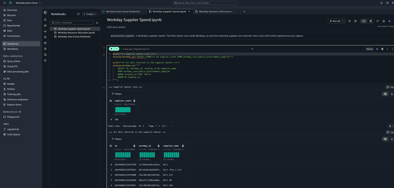
Amazon SageMaker Unified Studio notebook querying live Workday supplier data with Workday Live Data Query

Figure 1: Querying live Workday supplier data from an Amazon SageMaker Unified Studio notebook with Workday Live Data Query

Zero-copy federation with Apache Iceberg

For near real-time analytics, machine learning (ML) training, and large-scale data exploration, developers access Workday data through Workday Data Connect’s Apache Iceberg integration. By registering the Workday Iceberg REST Catalog in AWS Glue Data Catalog or AWS Lake Formation, all Workday datasets appear as standard Iceberg tables discoverable by any AWS analytics service. The compute runs on the customer’s AWS environment (using Athena, Amazon Redshift, Amazon EMR, or SageMaker AI) while the data stays in Workday Data Cloud.

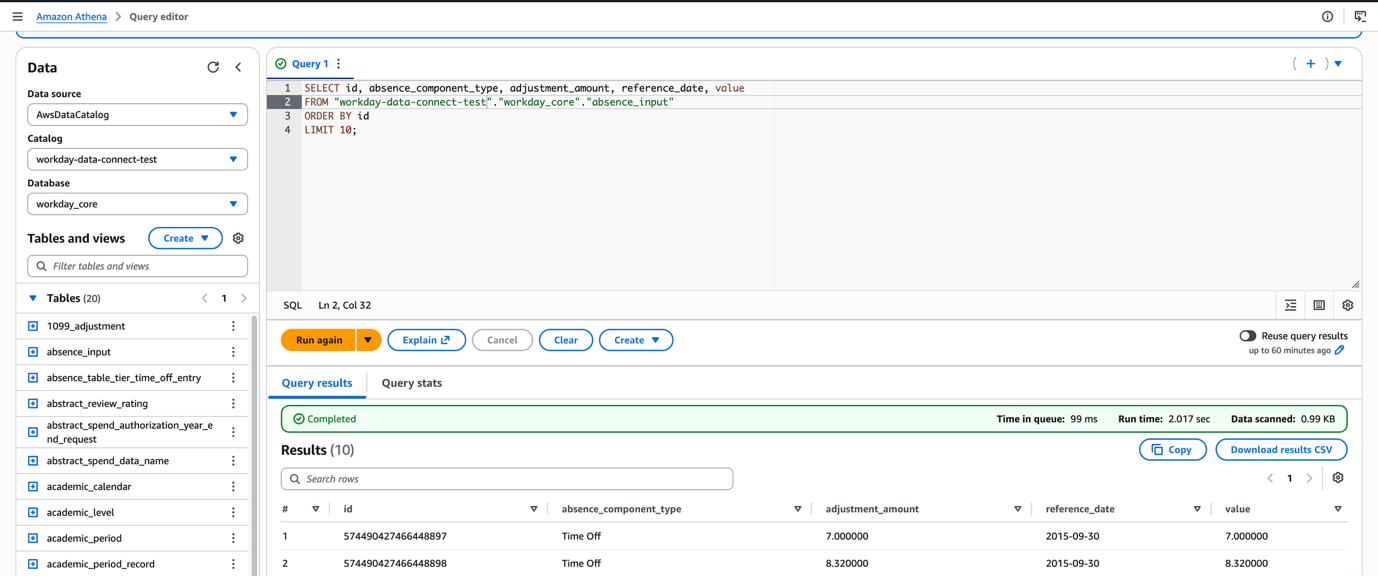
Amazon Athena query editor running standard SQL against a Workday Data Connect Iceberg table

Figure 2: Querying a Workday Data Connect Iceberg table with standard SQL in the Amazon Athena query editor

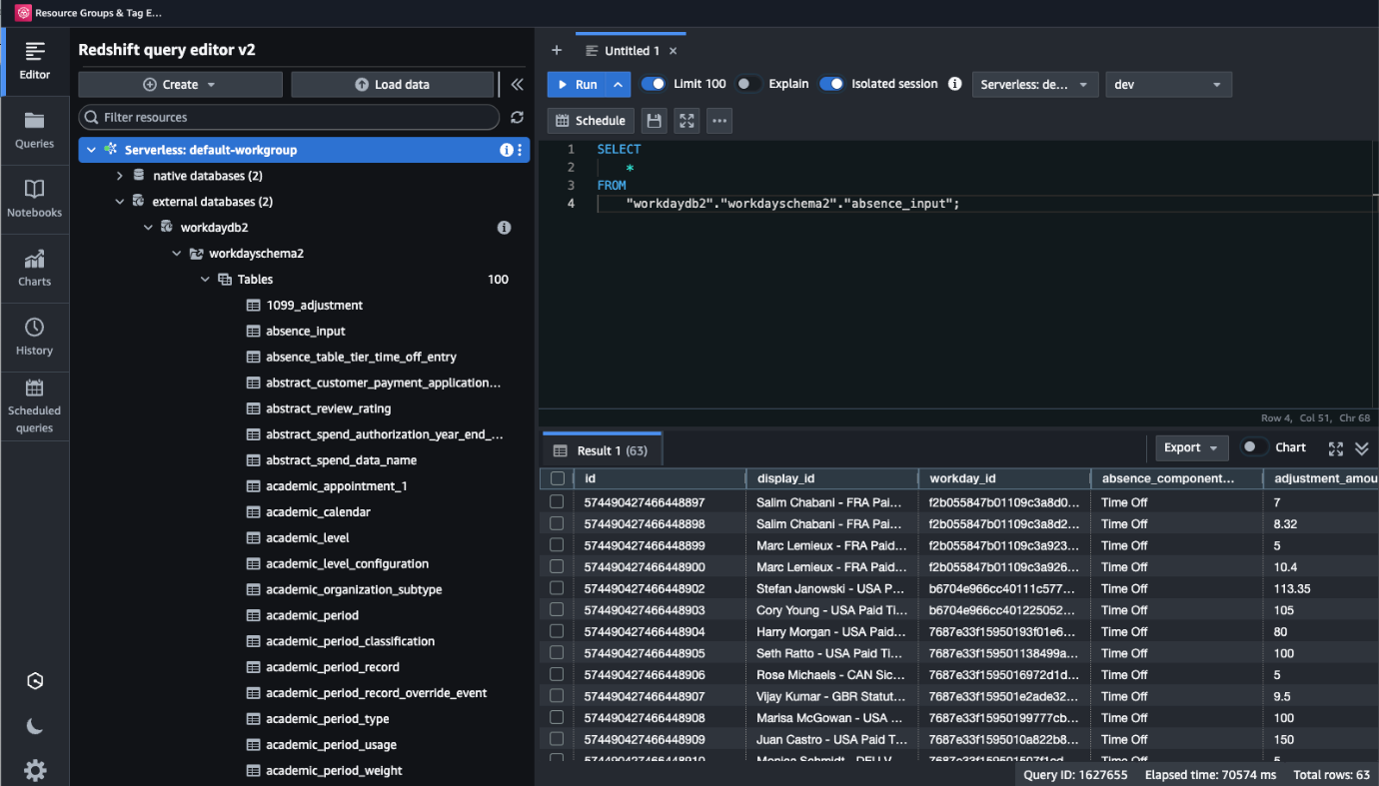
Querying a Workday Data Connect Iceberg table with standard SQL in the Amazon Athena query editor

Figure 3: Querying a Workday Data Connect Iceberg table with standard SQL in Amazon Redshift Query Editor v2.

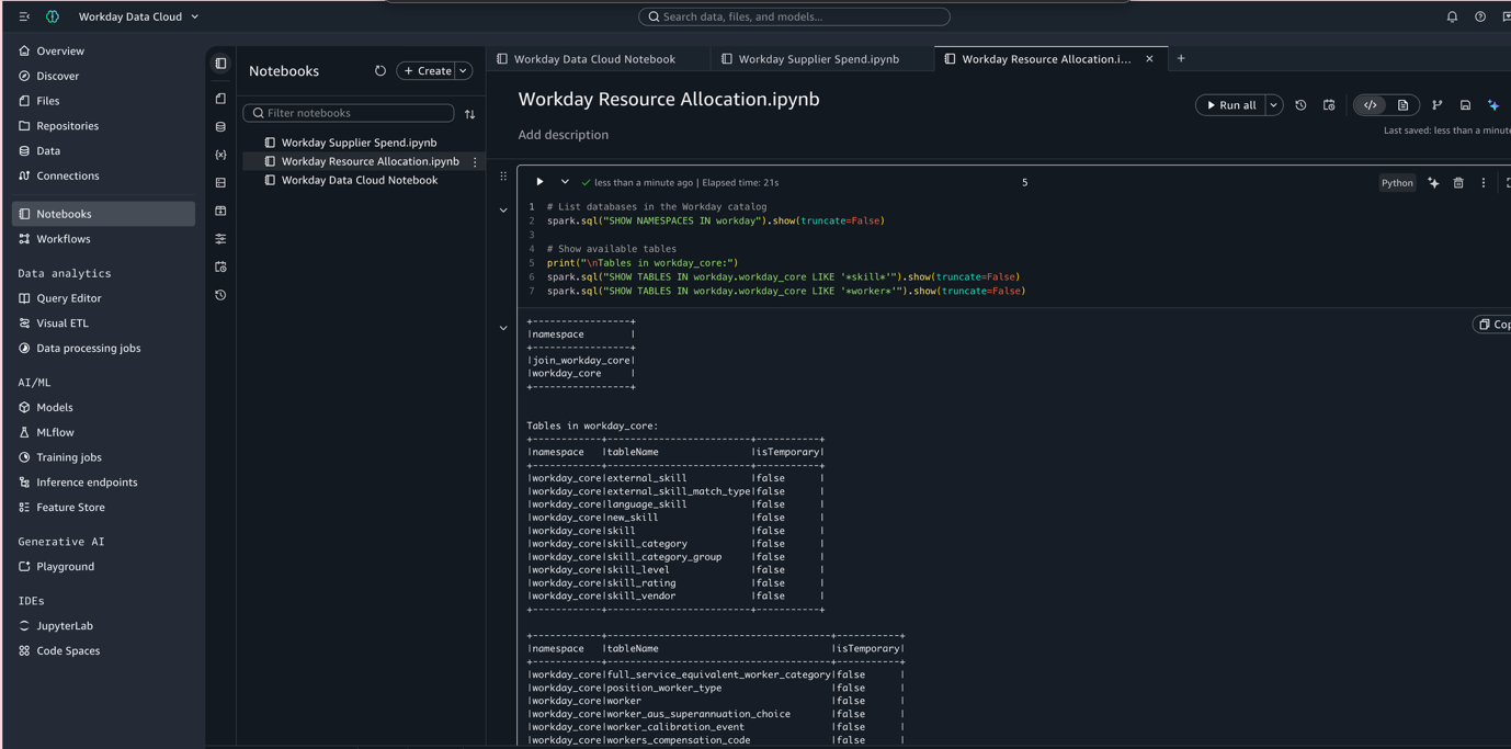
SageMaker Unified Studio notebook using PySpark to browse Workday Iceberg tables through Workday Data Connect

Figure 4: Browsing Workday Iceberg tables with PySpark in a SageMaker Unified Studio notebook using Workday Data Connect

What this means for customers

This integration changes how organizations work with their people and money data for analytics and AI. Here’s what it unlocks:

  • Organizations no longer need to build and maintain complex extract, transform, and load (ETL) pipelines to get Workday data into their analytics environment, which removes data silos without duplicating data. The data stays where it lives, governed and accurate, while remaining fully accessible for analysis and AI.
  • When AI agents and models can access Workday data with its full business context, developers spend less time reverse-engineering business logic and rebuilding permission models. That context includes who has access to what, what a metric actually means, and how calculations are defined.
  • Workday’s permission model, audit controls, and business logic travel with the data, and AWS Lake Formation adds governance on the AWS side. The result is data access that is both open and controlled, which is exactly what regulated industries and enterprise security teams require.
  • Instead of building pipelines, monitoring data freshness, and reconciling duplicates, data teams can focus on building analytics and machine learning applications that drive business outcomes.

Use case walkthrough: AI-powered workforce analytics

Consider a Chief People Officer who wants to understand the relationship between employee engagement scores, compensation benchmarks, and attrition patterns across the organization. Today, this requires extracting data from Workday, loading it into a separate analytics platform, joining it with market data, and building custom reports. This process takes weeks and produces stale results.

With the Workday Data Cloud and AWS integration, a data team can perform the following steps:

  1. Connect to Workday Data Cloud from AWS Glue using the pre-built Workday connector.
  2. Explore workforce datasets such as compensation, tenure, engagement, and performance directly, with full semantic context (job levels, org hierarchies, and tenure calculations) already defined.
  3. Join Workday people data with market compensation benchmarks and recruiting pipeline data stored as Iceberg tables on Amazon S3, all through standard SQL in Athena or SageMaker AI notebooks.
  4. Build a machine learning model in SageMaker AI that predicts attrition risk based on the combined dataset.
  5. Deploy an AI agent that flags high-risk attrition patterns for HR business partners to review and act on. The agent uses Live Data Query for near real-time signals and batch Iceberg access for historical trend analysis.

The entire workflow runs without any data leaving its governed environment, without any custom pipelines to maintain, and with full auditability at every step.

Getting started

The Workday Data Cloud integration with AWS is generally available.

  • Amazon SageMaker Unified Studio users can connect to Workday Data Cloud directly through the Workday Live Data Query connector or the Workday Iceberg REST Catalog connector.
  • Workday Live Data Query connections can also be created in the AWS Glue console, and users can query live Workday data from Amazon Athena, Amazon EMR, and AWS Glue ETL jobs.
  • AWS Glue and AWS Lake Formation users can register the Workday Iceberg REST Catalog as a federated catalog to make Workday datasets discoverable across AWS analytics services.
  • Workday users seeking to query AWS data can register their Glue Data Catalog Iceberg REST endpoint as an external catalog in Workday Data Cloud.

For deeper technical walkthroughs and step-by-step configuration guides, refer to the following resources:

This integration represents a new model for enterprise data access, where governed data flows freely between platforms without compromising security, accuracy, or business context. We are excited to see what customers build with Workday Data Cloud and AWS together.


About the authors

Poornima Chand

Poornima Chand

Poornima is a Principal Solutions Architect at AWS, where she works with customers to solve their unique challenges using AWS technology solutions. She is passionate about driving innovation in agentic AI and helping enterprises build intelligent, scalable, and secure solutions. Outside of work, she enjoys traveling, reading, painting, and spending time in nature.

Archana Bansal

Archana Bansal

Archana is a Senior Manager of Product Management for Workday Data Cloud, helping organizations unlock more value from their enterprise data and AI. Over more than six years, she has shaped the platform’s strategy and product direction, with a focus on data interoperability. She brings 20+ years of product leadership across enterprise data, analytics, and financial platforms at some of the industry’s largest product companies.

Avijit Goswami

Avijit Goswami

Based in California, Avijit is a Principal Data & Applied AI Architect at AWS who partners with customers to design and build robust data foundations and agentic AI solutions. When he’s not working, he loves hitting new trails, discovering new destinations, cheering on his favorite teams, listening to music, and trying out new recipes in the kitchen.

Will Cavin

Will Cavin

Will Cavin is a Principal Technical Product Manager working across the Data and Analytics teams at AWS. He has a passion for helping customers scale their analytics workloads. Prior to AWS, Will served as a cryptologist in the United States Navy. Based in Northern Virginia, he likes to long-distance run and mountain bike with his wife and son in his free time.

Tej Nagabhatla

Tej Nagabhatla

Tej is a Senior Solutions Architect at AWS. He has years of experience guiding numerous Fortune 500 companies along their technology journeys. He specializes in providing architectural guidance across a wide range of topics around AI/ML, security, storage, containers, and serverless technologies. In his free time, Tej enjoys spending time with family, playing basketball, and traveling.

Google TPU 8tx Pairs AMD EPYC Turin Hosts with Confidential Computing while TPU 8i Max Doubles Memory Bandwidth

Post Syndicated from Vic A original https://www.servethehome.com/google-tpu-8tx-8i-max-amd-epyc-turin/

The new Google TPU 8tx pairs AMD EPYC Turin hosts with confidential computing while TPU 8i Max doubles memory bandwidth for inference

The post Google TPU 8tx Pairs AMD EPYC Turin Hosts with Confidential Computing while TPU 8i Max Doubles Memory Bandwidth appeared first on ServeTheHome.

Transforming fleet analytics for Novus Hi-Tech through agentic AI

Post Syndicated from Sameer Shrivastava original https://aws.amazon.com/blogs/architecture/transforming-fleet-analytics-for-novus-hi-tech-through-agentic-ai/

Fleet analytics sounds straightforward until you have thousands of vehicles streaming dashcam footage, driver alerts, GPS pings, and speed warnings across 10 countries, all at the same time. At that scale, no team can manually triage every drowsiness alert or investigate every over-speeding event before it becomes a real incident. With over 120 enterprise customers relying on their fleet, Novus Hi-Tech needed a system that would act on the data, not only show it. With AI-powered automation, they achieved a 46 percent reduction in road-behavior violations and a 55 percent drop in drowsiness alerts per 1,000 km.

In this post, we walk you through how Novus Hi-Tech, in collaboration with the AWS Prototyping and AI Customer Engineering (PACE) team, designed and implemented an agentic AI solution called FleetGPT. We architected the multi-agent system using Strands Agents SDK and AWS managed AI services, turning IoT data into real-time safety interventions through natural language querying, automated investigation, and AI-powered voice calls to drivers.

For years, extracting value from fleet telemetry required significant manual effort. When a drowsiness alert triggered, operators had to validate video footage, assess severity across multiple signals, contact the driver, and log the outcome. Existing fixed dashboards showed the same views regardless of what teams actually needed to know.

At scale, this model breaks down because one can’t staff enough operators to catch every warning in real time, and manual analysis becomes the bottleneck. The cost of a missed warning could be a preventable accident.

Novus Hi-Tech needed a system that understood the difference between what a fleet manager needs to know, what a customer success analyst is looking for, and what a Command Center operator must act on immediately.

The bottleneck

The friction between question and answer wasn’t uniform. It created different bottlenecks depending on what teams were trying to accomplish.

Every warning that reached the Command Center demanded the same judgment calls. Operators cycled through this decision tree hundreds of times per shift.

On the other hand, fleet managers didn’t need individual event response, but pattern recognition: which drivers are trending toward accidents, which routes carry disproportionate risk, which fleets are drifting on safety compliance.

Both roles shared the same friction: the time between asking a question and getting an answer. Operators spent too long investigating individual events. Fleet managers couldn’t analyze trends fast enough. Neither could move from question to insight without switching tools or waiting on data teams.

Solution overview

FleetGPT replaces fixed dashboards with a natural language interface for dynamic querying, investigation, and insight generation. It surfaces video evidence, driver history, and policy in single interactions. Beyond analytics, FleetGPT automates real-time safety interventions. When a critical event occurs, such as repeated drowsiness, over-speeding, or an SOS trigger, the system initiates a two-way AI-powered voice call in the driver’s native language, with user approval. It tracks acknowledgment and escalates when necessary.

FleetGPT is built with two core capabilities.

  1. Analyst: A conversational intelligence layer where operators and fleet managers query the fleet data, retrieve video evidence, and search policy documents through natural language.
  2. Intervention engine: An agentic layer that monitors incoming events, evaluates severity, and executes driver interventions with human approval.

Analyst: Natural language intelligence

Novus Hi-Tech’s data landscape included separate systems for telemetry, video, and policy documents. FleetGPT unifies these through a single data layer accessed by an agentic conversational interface.

Data storage and processing layer

Data store Role Key design choice
Amazon Aurora PostgreSQL Structured data Stores structured telemetry data
Amazon DynamoDB High velocity event stream from devices Low latency read-write operations with composite keys optimized for agentic query patterns
Amazon Bedrock Knowledge Bases Implement RAG with agentic system Vector embeddings stored in Aurora PostgreSQL with pgvector for semantic retrieval

Amazon Aurora PostgreSQL manages the structured analytical backbone. It stores per-vehicle daily aggregates covering distance, fuel, safety scores, event counts, and GPS statistics, plus live snapshots of current vehicle status. It’s the primary target for the Text-to-SQL pipeline. A YAML schema file with column aliases, descriptions, and worked examples is injected into every SQL generation prompt. This grounds the large language model (LLM) on the actual schema and reduces hallucination on column names and join paths.

Amazon DynamoDB handles the high-velocity warning event stream. The warning event table uses a composite sort key of warning_code + datetime, enabling efficient range queries by warning type and time window without full table scans. A Global Secondary Index on fleet_id supports fleet-scoped queries without touching data from other tenants. A separate device registry table maps vehicle IDs to country metadata which is the source of truth for language routing in audio alerts.

Amazon Bedrock Knowledge Bases, the fully managed RAG capability, indexes unstructured documents including SOPs, compliance policies, product documentation which are stored in Amazon Simple Storage Service (Amazon S3). The embeddings are generated using Amazon Titan Text Embeddings V2 for storage in Amazon Aurora PostgreSQL with pgvector. This gives operators and fleet managers a single interface for both data questions and policy questions, with no context switching.

Orchestration: Strands Agents

FleetGPT multi-agent architecture over Amazon Aurora, DynamoDB, and Amazon Bedrock Knowledge Bases

Figure 1: Solution architecture

The system uses a multi-agent architecture built with Strands Agents, where each agent has a distinct role and model assignment based on the complexity of its task.

At the top sits the Supervisor agent, running on Claude Sonnet 4.6 (for model availability by AWS Region, refer to Region availability by models), which handles intent decomposition and multi-step reasoning. It decides what kind of question the user is asking and routes it to the right sub-agent. The Supervisor uses a SummarizingConversationManager from Strands Agents, which preserves the last six messages verbatim while summarizing older turns. This keeps context window usage bounded without losing conversational continuity.

For structured data queries, the Supervisor delegates to a Text-to-SQL sub-agent (also Claude Sonnet 4.6). This agent follows a plan-and-execute approach: it first classifies the query type (vehicle data, driver behavior, or operational metrics), then extracts key entities and maps them to database tables and columns. From there, it generates a query plan outlining the relevant tables and operations, and finally produces and executes the SQL. If an error occurs, the agent retries with the error message, original plan, and failed query included in the prompt for self-correction.

Text-to-SQL sub-agent flow: classify the query, extract entities, map to tables, generate a plan, then produce and run SQL

Figure 2: Text-to-SQL sub-agent flow

When a query needs computation beyond SQL (correlation analysis, statistical profiling, trend detection), the Supervisor delegates to a Data Processing sub-agent running on Claude Haiku 3.0 (for model availability by AWS Region, refer to Region availability by models). Rather than pushing complex processing onto the database, this agent generates executable Python, runs it through a Python REPL tool, and returns the shaped results to the orchestrator. Claude Haiku 3.0, a smaller model than Claude Sonnet 4.6, helps keep the inference cost down for this tier of the pipeline.

Each agent has a focused tool surface and scoped system prompt, reducing hallucination and making failures straightforward to isolate.

The agent is hosted on AWS Fargate for Amazon Elastic Container Service (Amazon ECS), which provides a serverless container environment. An Application Load Balancer (ALB) serves as the entry point, routing incoming requests to the ECS-hosted application.

Video evidence retrieval

Video retrieval demonstrates the practical impact of this architecture. Earlier retrieving dashcam footage required operators to know vehicle IDs, navigate a separate system, and apply filters manually.

Operators now retrieve video using natural language, specifying fleet, vehicle, warning type, date range, speed, or city. The agent resolves these parameters into a DynamoDB query using the composite sort key, applies the remaining criteria as in-memory filters, and returns a paginated result set with vehicle ID, timestamp, GPS coordinates, and a streamable video link in a single conversation.

Multi-tenancy and conversation persistence

Multi-tenancy is enforced at the data layer. Every query is scoped to the authenticated user’s authorized fleet IDs, injected into the agent’s context at session initialization. This helps reduce the risk of cross-tenant data access, whether through natural language, prompt injection, or direct tool calls.

Conversation history is stored in DynamoDB with a composite key of user_id + conversation_id + timestamp, to support per-user time-ordered retrieval. At session start, the system also injects live operational context including today’s warning counts, the latest critical events and the currently open video. This gives the agent situational awareness along with the conversation history.

Intervention engine: Automated event response

The intervention agent acts on critical events. When warnings such as drowsiness, dangerous speeding, or SOS arrive, the system evaluates severity and queues interventions for user approval.

Real-time event push through Amazon DynamoDB Streams

ADAS (Advanced Driver Assistance Systems) edge devices send warning events to DynamoDB. Amazon DynamoDB Streams capture these events, which a background worker forwards to the notification API for delivery to the Command Center.

The worker uses exponential backoff on idle periods: if no new events are found, the poll interval doubles up to a maximum of five minutes, then resets to the base interval on the next event. A fallback polling job provides redundancy, scanning a configurable recent time window on a fixed schedule in case the stream worker misses an event.

Two-way AI voice calling

When a safety event needs direct driver contact, the system automatically initiates a fresh conversation session that is pre-configured with the driver’s language. The LLM system prompt, STT/TTS voice model, and language hint are all set at session start. You can refer to Sample Indic Language Voicebot for reference implementation.

The voice calling pipeline operates in real time:

  1. Speech-to-Text: The driver’s voice is captured through the in-cabin microphone and transcribed by a high-accuracy multilingual STT (Speech-to-Text) model, with the language hint set at the beginning of the session for accuracy across regional fleets.
  2. LLM Processing: Transcriptions are sent to an LLM on Amazon Bedrock that generates contextually appropriate responses in the driver’s native language.
  3. Text-to-Speech and delivery: Responses are synthesized using a multilingual TTS (Text-to-Speech) model and streamed to the vehicle’s IVI (In-Vehicle Infotainment) head unit over WebSocket.
  4. Interrupt handling: VAD (Voice Activity Detection) monitors for driver speech during system responses, immediately canceling active streams to allow natural conversation flow.

Key design decisions

Building FleetGPT required deliberate choices about frameworks, data stores, and agent architecture. The following sections explain the reasoning behind the decisions that shaped the system.

Why Strands Agents?

Strands Agents was chosen for fine-grained control over tool invocation, conversation lifecycle management, and per-session agent state within a Python-native environment. Capabilities such as summarizing conversation memory, multi-model routing, and caching intermediate tool outputs are easier to implement and tune directly at the SDK level than through higher-level abstraction layers.

DynamoDB

Amazon DynamoDB provides the low-latency reads and stream processing needed for real-time fleet monitoring. The composite sort key design deliberately matches agent query patterns to allow efficient filtering without table scans. A Global Secondary Index on fleet_id helps provide tenant isolation. Amazon DynamoDB Streams trigger the intervention pipeline so the system reacts to critical safety events within seconds.

Amazon Bedrock

Amazon Bedrock provides the foundation model infrastructure for FleetGPT, offering access to multiple models. Amazon Bedrock Knowledge Bases handles the complete RAG pipeline for policy and documentation retrieval, alleviating the need for custom RAG infrastructure while maintaining the security and access controls already established for structured data.

Sub-agent delegation for specialization without coupling

The three-tier data analysis chain exists because each step requires fundamentally different reasoning. Consolidating these responsibilities into a single agent would degrade performance across multiple dimensions.

A monolithic agent must balance competing concerns in its system prompt, reducing effectiveness for each task. It must select from a larger tool inventory, increasing decision complexity and error rates. And when failures occur, diagnosing the root cause becomes significantly harder.

Separating these concerns means each agent can be prompted, tested, and improved independently, with clear failure boundaries at each tier.

Atomic system prompts for maintainability and debugging

System prompts are structured as composable, tagged instruction blocks rather than a monolithic string. Each instruction is a discrete, auditable unit which is tagged by category, named, and independently editable. When two instruction blocks produce conflicting behavior, the tag and block name tell you exactly where to look, without having to reason about the prompt as a whole. This made iterating on specific behaviors fast and safe.

Results

FleetGPT has delivered measurable operational impact across Novus Hi-Tech’s customer base:

  1. 46 percent annual reductions in road-behavior violations.
  2. Insights from data led to a 3–6 percent increase in fuel efficiency.
  3. 55 percent reduction in drowsiness alerts per 1,000 km.

These improvements stem from four key operational transformations:

  1. Warning validation time dropped from minutes to seconds: Investigating a single warning previously meant navigating multiple dashboard screens, manually filtering video feeds, cross-referencing driver history in separate tools, and looking up policy documents. Now it’s a single conversational query that surfaces video evidence, driver history, and fleet context together.
  2. Real-time alert delivery within seconds: The DynamoDB Streams based pipeline replaced a polling-based system with multi-minute latency. Command Center operators now receive critical warnings within seconds of an event being recorded by an edge device in the field.
  3. Self-service analytics for fleet managers: Fleet managers generate driver performance reports, fleet health summaries, and trend analyses without engaging the data team. Questions that once took hours or days are now answered in conversational turns.
  4. Improved driver response rates in multilingual fleets: Delivering audio alerts in each driver’s native language has measurably improved acknowledgment rates across regional fleet segments, where a single-language approach previously left a significant portion of drivers underserved.

Conclusion and next steps

FleetGPT demonstrates how agentic AI can transform operational workflows when applied to domain-specific problems. By combining natural language interfaces with automated intervention systems, Novus Hi-Tech moved from reactive dashboard monitoring to proactive, context-aware fleet management.

Looking ahead, Novus Hi-Tech is expanding FleetGPT’s capabilities in three directions:

Amazon Bedrock AgentCore: Host the developed agent on Amazon Bedrock AgentCore, a platform to build, connect, and optimize agents at scale, with any framework or model.

Predictive risk scoring: The dataset now carries enough behavioral history to surface vehicles trending toward incidents before they occur. The next capability will score drivers against their own baselines and flag deteriorating patterns proactively.

Embedded chart and visualization generation: Fleet managers think visually. Rather than returning tabular data, the agent will embed generated charts directly in responses for trend queries which will close the gap between insight and presentation without a separate business intelligence tool in the loop.

If you manage real-time operational data across distributed systems, FleetGPT offers a blueprint: start with the questions your teams ask most often, build agents that can answer them reliably, and then extend those agents to act on the answers.

For more information and relevant reads, see the following resources:


About the authors

Define metrics once and keep them correct with the dbt Semantic Layer on Amazon Redshift

Post Syndicated from Isabelly Rocha original https://aws.amazon.com/blogs/big-data/define-metrics-once-and-keep-them-correct-with-the-dbt-semantic-layer-on-amazon-redshift/

Most analytics stacks model data into a curated gold layer and call the result a semantic layer. For a lot of workloads, that’s a perfectly good one. The business logic lives in version-controlled models, every consumer reads the same tables over SQL, and there’s no extra product to run. The honest position is that a well-modeled gold layer is a semantic layer for standardizing metrics, and reaching for a dedicated tool before you need one is over-engineering.

This post is about the point where that stops being true: when users need to compute a metric across arbitrary combinations of dimensions, chosen at query time, and some of those metrics are non-additive. We will first show, with real numbers, why pre-aggregated gold tables produce silently wrong results in that case. Then we will build a working solution on Amazon Redshift using the open-source dbt Semantic Layer (powered by MetricFlow), define average_order_value once, and prove it stays correct whether you slice it by day, by week, or by store.

A quick note on where this fits on AWS. Semantic and metric definitions on AWS have generally lived downstream of the warehouse rather than inside it. Amazon Quick Sight Topics define metrics for Quick Sight dashboards and Amazon Q. The newer AWS Context service builds a knowledge-graph layer over the AWS Glue Data Catalog to attach business meaning to data assets for agents and downstream tools (overview). Those are the places to watch as that story matures. This post stays deliberately narrow on a different, less-documented need: a governed metric layer you define once in Git, right next to your Amazon Redshift models, and query correctly from any tool. You build it with open-source dbt and MetricFlow.

The problem: Where a gold layer stops short

Limitation 1: The combinatorial wall

A gold table is pre-aggregated at one grain. To let users slice a metric by any combination of dimensions, you need a pre-built table per combination, and that count explodes as 2ⁿ:

Dimensions you let users mix Pre-aggregated shapes you’d need
2 (region, week) 4
3 (+ channel) 8
5 (+ product category, segment) 32
7 (+ device, campaign) 128

Nobody builds 128 tables. You build the dozen someone asked for and field a ticket for every new slice. The escape hatch is to expose one wide fact table and let each business intelligence (BI) tool do its own GROUP BY. That restores flexibility, and it walks straight into the second, nastier problem.

Limitation 2: The metric is wrong, and nobody notices

Many everyday BI metrics are non-additive: you can’t roll them up by averaging the sub-totals. Average order value is the one nearly every dashboard has.

Suppose one store had these orders in a week:

day order amount
Mon #1 $1,000
Tue #2 $100
Tue #3 $100
Tue #4 $100
Tue #5 $100

Your gold table is pre-aggregated to a daily grain, because that’s what the daily sales dashboard needed:

day orders revenue avg_order_value
Mon 1 $1,000 $1,000
Tue 4 $400 $100

Now someone asks a new question: “What was the average order value this week?” The BI tool only has the daily gold table, so it averages the two daily numbers:

($1,000 + $100) / 2  =  $550     [WRONG] looks fine, is wrong

The real answer, from the actual orders, is:

total revenue / total orders  =  $1,400 / 5  =  $280     [CORRECT] the truth

The naive rollup reports $550, nearly double the real $280. Nobody sees the error, because $550 is a plausible-looking number. The daily averages were each correct. Averaging them was the mistake. The weekly figure has to be recomputed as SUM(revenue) / COUNT(orders) at the week grain, and a pre-aggregated daily table doesn’t carry what’s needed to do that. Conversion rate, profit margin, cost per acquisition, and distinct counts all share this trap.

The requirement, then, isn’t “standardize the columns.” It’s: define the metric and its aggregation rules once, and compute them correctly on the fly for any dimensions a user picks. That’s exactly what the dbt Semantic Layer does, and the rest of this post builds it on Amazon Redshift.

Solution overview

We will put the metric definition in a dbt project, with Amazon Redshift as the warehouse. dbt builds the gold model. MetricFlow turns metric definitions in YAML into correct, grain-aware SQL at query time.

Architecture diagram showing dbt building the fct_orders model on Amazon Redshift and the dbt Semantic Layer (MetricFlow) generating grain-aware SQL for the mf query CLI, generated SQL, and BI tools such as Lightdash and Amazon Quick Sight

Figure 1: Architecture of the dbt Semantic Layer on Amazon Redshift

We keep the dataset deliberately tiny: only the five orders shown earlier. You can verify every number by hand and watch the week-grain result come back as $280, not $550.

The full dbt project and the AWS Cloud Development Kit (AWS CDK) app used in this walkthrough live in the companion repository, sample-dbt-semantic-layer-on-amazon-redshift: the dbt project under dbt/ and the Redshift Serverless CDK app under infra/. The repo also ships deploy, destroy, and end-to-end test scripts. See its README for a one-command runbook.

Prerequisites

  • An AWS account with permission to create an Amazon Redshift Serverless workgroup (or an existing Amazon Redshift cluster) and query it.
  • An Amazon Redshift database and schema you can write to, plus the connection endpoint, user, and password. (AWS Identity and Access Management (IAM), or IAM, authentication also works. This walkthrough uses a user and password for brevity.)
  • Python 3.9–3.12 and pip.
  • Basic familiarity with the command line and dbt.

Estimated cost: A Redshift Serverless workgroup with 8 RPUs (Redshift Processing Units) bills about $3/hour of active query time (metered per second, with a 60-second minimum per query), so a short walkthrough like this typically costs under a dollar. Follow the Clean up section to avoid ongoing charges.

Step 1: Provision Amazon Redshift and note the connection details

If you don’t already have an Amazon Redshift endpoint, create a Redshift Serverless workgroup from the console (Amazon Redshift → Redshift Serverless → Create workgroup). Note the workgroup’s endpoint, the database name (default dev), and the admin user and password you set.

Amazon Redshift Serverless workgroup page showing the endpoint and database name

Figure 2: The Redshift Serverless workgroup detail page with its endpoint, port 5439, and database dev

If you prefer infrastructure-as-code, use the AWS CDK app in the companion repo’s infra/. Set your target account and AWS Region, then run the provided deploy script, which scopes inbound access to your current IP:

export CDK_DEFAULT_ACCOUNT=<your-account-id> CDK_DEFAULT_REGION=<your-region>
./scripts/deploy.sh

Read the generated admin password from AWS Secrets Manager (the script prints the secret name). An overly broad CIDR such as 0.0.0.0/0 is rejected unless you explicitly opt in. The preceding console steps remain valid.

Open Query Editor v2 and create a schema for this project:

CREATE SCHEMA IF NOT EXISTS semantic_demo;

Step 2: Set up the dbt project

Create and activate a virtual environment, then install the dbt adapter for Amazon Redshift and MetricFlow. Installing dbt-redshift brings a compatible dbt-core (1.9+ is required for the time-spine YAML used later), and dbt-metricflow adds the mf CLI:

python -m venv .venv
source .venv/bin/activate
pip install "dbt-redshift==1.9.5" "dbt-metricflow==0.11.0"

These versions are pinned so the walkthrough matches the output shown here. dbt-metricflow currently resolves dbt-core to the 1.10.x line. Newer dbt-core releases print a deprecation notice during dbt debug but behave the same for this project. If you prefer to stay current, install the latest dbt-redshift and dbt-metricflow. The metric definitions in Step 4 are unchanged.

Initialize a project:

dbt init aov_demo
cd aov_demo

Want the exact runnable project used here instead of building from scratch? Clone the companion repo. Its dbt project and profile are both named semantic_demo. Copy dbt/profiles.example.yml to ~/.dbt/profiles.yml rather than running dbt init aov_demo. You can also reproduce the entire walkthrough end to end with ./scripts/e2e-test.sh.

Configure the connection in ~/.dbt/profiles.yml (replace the placeholders with your workgroup values):

aov_demo:
  target: dev
  outputs:
    dev:
      type: redshift
      host: <your-workgroup>.<account>.<region>.redshift-serverless.amazonaws.com
      user: admin
      password: "{{ env_var('REDSHIFT_PASSWORD') }}"
      port: 5439
      dbname: dev
      schema: semantic_demo
      threads: 4
      sslmode: require

Export the password and confirm the connection:

export REDSHIFT_PASSWORD='<your-password>'
dbt debug
Terminal showing dbt debug with all connection checks passing

Figure 3: The dbt debug command confirms the Amazon Redshift connection, with all checks passing

Add dbt_utils (used for the time spine MetricFlow needs) in packages.yml:

packages:
  - package: dbt-labs/dbt_utils
    version: [">=1.0.0", "<2.0.0"]
dbt deps

Step 3: Seed the sample orders and build the gold model

Create seeds/raw_orders.csv with the exact five orders from the problem section (Jan 5, 2026 is a Monday and Jan 6 a Tuesday, in the same ISO week):

order_id,store,ordered_at,amount
1,downtown,2026-01-05,1000
2,downtown,2026-01-06,100
3,downtown,2026-01-06,100
4,downtown,2026-01-06,100
5,downtown,2026-01-06,100

Load it into Amazon Redshift:

dbt seed

Create the gold model models/marts/fct_orders.sql:

{{ config(materialized='table') }}

select
    order_id,
    store,
    cast(ordered_at as date) as ordered_at,
    amount
from {{ ref('raw_orders') }}

Create the time spine MetricFlow uses to reason about dates, models/marts/metricflow_time_spine.sql:

{{ config(materialized='table') }}

with days as (
    {{ dbt_utils.date_spine(
        datepart="day",
        start_date="cast('2026-01-01' as date)",
        end_date="cast('2026-02-01' as date)"
    ) }}
)

select cast(date_day as date) as date_day
from days

Register the time spine in models/marts/_models.yml:

models:
  - name: metricflow_time_spine
    time_spine:
      standard_granularity_column: date_day
    columns:
      - name: date_day
        granularity: day

Build everything:

dbt run
Query Editor v2 showing the fct_orders table with five rows

Figure 4: The five seeded orders in the fct_orders table, queried from Amazon Redshift Query Editor v2

Step 4: Define the semantic model and the metric (once)

This is the heart of it. Create models/marts/sem_orders.yml. The semantic model declares the entities, dimensions, and measures. The metric declares average_order_value as a ratio of two metrics (total_revenue over order_count), so MetricFlow always computes it as SUM(amount) / COUNT(orders) at whatever grain is requested:

semantic_models:
  - name: orders
    model: ref('fct_orders')
    defaults:
      agg_time_dimension: ordered_at
    entities:
      - name: order
        type: primary
        expr: order_id
    dimensions:
      - name: store
        type: categorical
      - name: ordered_at
        type: time
        type_params:
          time_granularity: day
    measures:
      - name: order_total
        description: Sum of order amounts.
        agg: sum
        expr: amount
      - name: order_count
        description: Number of orders.
        agg: count
        expr: order_id

metrics:
  - name: average_order_value
    label: Average order value
    description: Average revenue per order. Non-additive ratio.
    type: ratio
    type_params:
      numerator: total_revenue
      denominator: order_count
  - name: total_revenue
    label: Total revenue
    description: Total order revenue.
    type: simple
    type_params:
      measure: order_total
  - name: order_count
    label: Order count
    description: Count of orders.
    type: simple
    type_params:
      measure: order_count

Parse the project so MetricFlow picks up the definitions, then validate them:

dbt parse
mf validate-configs
mf list metrics
Terminal showing mf list metrics with average_order_value, total_revenue, order_count

Figure 5: The mf list metrics command showing the three governed metrics and the dimensions each can be sliced by

Step 5: Query the metric at two grains (the payoff)

First, average order value by day:

mf query --metrics average_order_value --group-by metric_time__day --order metric_time__day
metric_time__day    average_order_value
-------------------  --------------------
2026-01-05           1000.00
2026-01-06           100.00

Now the same metric by week, which is the exact question that broke the gold table earlier:

mf query --metrics average_order_value --group-by metric_time__week
metric_time__week    average_order_value
-------------------  --------------------
2026-01-05           280.00

$280, not $550. You changed one word (day → week) and the metric stayed correct, because MetricFlow recomputed SUM(amount) / COUNT(orders) at the week grain instead of averaging daily averages. Show the supporting numbers to make it obvious:

mf query --metrics total_revenue,order_count,average_order_value --group-by metric_time__week
metric_time__week    total_revenue    order_count    average_order_value
-------------------  ---------------  -------------  --------------------
2026-01-05           1400.00          5              280.00

And the combinatorial point: the same metric sliced by a completely different dimension, with no new table built:

mf query --metrics average_order_value --group-by order__store
Terminal showing the day-grain and week-grain mf query results side by side

Figure 6: The same metric by day ($1,000 and $100) and by week ($280), recomputed from the raw orders rather than averaged from the daily values

Step 6: See the generated SQL and consume the metric

To see that MetricFlow is doing the right thing, ask it for the SQL instead of the result:

mf query --metrics average_order_value --group-by metric_time__week --explain

The rendered SQL (abbreviated) sums and counts at the requested grain rather than averaging a pre-aggregate:

select
    date_trunc('week', ordered_at)        as metric_time__week,
    sum(amount)                            as order_total,
    count(order_id)                        as order_count,
    sum(amount) / nullif(count(order_id), 0) as average_order_value
from semantic_demo.fct_orders
group by 1

Because this is dbt Core (open source), consumption options are:

  • The mf query CLI shown earlier — for validation, notebooks, and scripts.
  • mf query --explain to lift the generated SQL into any tool, scheduler, or materialized model.
  • A BI tool that reads the MetricFlow semantic manifest (semantic_manifest.json, produced by dbt parse), for example Lightdash’s dbt MetricFlow integration, so dashboards query the governed metric instead of re-deriving it.
  • A BI tool with no first-class Semantic Layer connector, such as Amazon Quick Sight: materialize the metric back into Amazon Redshift and point the tool at it. In open-source dbt you can wrap MetricFlow’s generated SQL (mf query --explain) in a dbt model. On dbt Cloud, a saved query with an export writes the result to a table or view on a schedule. Either way the metric is still defined once in the semantic layer. Quick Sight only reads an ordinary Amazon Redshift table.

The fully hosted dbt Semantic Layer API requires dbt Cloud. This is the API that BI tools like Tableau and Power BI connect to over a JDBC/GraphQL endpoint. The metric definitions are identical. Only the serving layer differs. If you later move to dbt Cloud, the YAML from Step 4 is unchanged.

Clean up

To avoid ongoing charges:

  1. Drop the demo schema in Amazon Redshift:
    DROP SCHEMA IF EXISTS semantic_demo CASCADE;

  2. If you created a Redshift Serverless workgroup solely for this walkthrough, delete it. With the companion repo, run ./scripts/destroy.sh --yes (or make destroy). From the console: Amazon Redshift → Redshift Serverless → select the workgroup → Delete, then delete its namespace.
  3. Deactivate or remove the local virtual environment if you no longer need it.

Conclusion

A well-modeled gold layer is a legitimate semantic layer, and for stable, additive metrics it’s the right, low-cost default. The clear trigger to add a query-time semantic layer is the case we built here: metrics sliced across many dimensions in combinations you can’t pre-enumerate, where non-additive measures silently break when a BI tool rolls them up. The dbt Semantic Layer removes the choice between combinatorial table sprawl and wrong numbers. You define average_order_value once, in version-controlled YAML, and MetricFlow generates correct SQL on Amazon Redshift for every grain and dimension.

From here you can add more metrics (cumulative, derived, conversion), wire the semantic manifest into an open source BI tool, or graduate to dbt Cloud for the hosted API that major BI tools connect to directly. None of this changes the metric definitions.

Further reading


About the author

Isabelly Rocha

Isabelly Rocha

Isabelly is a Solutions Architect at AWS based in Zurich, Switzerland, where she helps enterprise customers design and build scalable, high-performing analytics solutions. She holds a PhD in Computer Science, where her research focused on distributed systems and cloud computing — work she later applied directly during three years as a Software Development Engineer on the Amazon Redshift team. She is passionate about helping customers get the most out of their data on AWS.

How DeepL keeps closest-exit routing during maintenance with AWS Cloud WAN

Post Syndicated from Guzman Freigedo original https://aws.amazon.com/blogs/architecture/how-deepl-keeps-closest-exit-routing-during-maintenance-with-aws-cloud-wan/

DeepL is a Language AI company that builds written and real-time AI voice translation products used by more than 200,000 business teams worldwide. Its infrastructure spans multiple AWS Regions across Europe, North America and Asia, with hybrid connectivity back to two European data centers.

Taking a single AWS Direct Connect link out of service for planned maintenance is a routine task, but in a multi-Region hybrid network it demands care. DeepL connects its AWS Regions to its data centers through Direct Connect and relies on the default closest-exit egress behavior to keep latency low. For maintenance, the team’s goal was to drain one link while every other Region continued using its local exit.

This post describes how DeepL does this with AWS Cloud WAN and a Direct Connect gateway attached natively to the core network. An AS_PATH prepend on the link being maintained moves only that Region’s traffic to another location, and the other Regions keep their local exit. It also covers the trade-offs, including inter-Region data transfer while a link is drained.

This post is for network architects and cloud platform teams who operate hybrid connectivity at scale, who are evaluating AWS Cloud WAN for global routing, or who are working through Direct Connect traffic engineering across Regions.

DeepL’s hybrid architecture

DeepL runs workloads in multiple AWS Regions, including three in Europe (eu-west-1 in Ireland, eu-central-1 in Frankfurt, and eu-north-1 in Stockholm), two in the United States (us-east-1 and us-west-2), and one in Tokyo (ap-northeast-1). Each Region has multiple virtual private clouds (VPCs) and accounts. On premises, two European data centers connect over a resilient Multiprotocol Label Switching (MPLS) network with dedicated fiber between the sites.

The connectivity design is built for geographic redundancy:

  • Three AWS Direct Connect locations (Dublin, Copenhagen, and Stockholm), each with a hosted 25 Gbps connection through AWS Direct Connect Partner Megaport.
  • An AWS Cloud WAN core network with a core network edge (CNE) in multiple Regions that connects the VPCs and accounts in that Region.
  • One global Direct Connect gateway, linked to all three Direct Connect locations and attached natively to the core network. Native Direct Connect gateway attachments for AWS Cloud WAN have been available since November 2024.
  • The same prefixes advertised from the on-premises routers in both data centers, so that the Direct Connect gateway learns them over all three Direct Connect locations (simplified here to a single /16).

The following diagram shows this architecture.

DeepL’s hybrid architecture: AWS Regions connected through an AWS Cloud WAN core network, a Direct Connect gateway, three Direct Connect locations, and two on-premises data centers advertising the same /16

Figure 1: DeepL’s hybrid architecture with AWS Cloud WAN

In steady state, DeepL runs no additional traffic engineering. By default, egress traffic leaves AWS through the Direct Connect location closest to where it originated: traffic from eu-west-1 leaves through Dublin, traffic from eu-central-1 through Copenhagen, and traffic from eu-north-1 through Stockholm. This closest-exit behavior keeps latency low and avoids extra configuration.

DeepL wanted to take the router at one Direct Connect location out of service for a maintenance window. Traffic had to move off that single link while the other two locations kept serving their Regions as before. This is a common requirement for enterprises running multiple Direct Connect locations.

Where the egress decision is made

Before changing any Border Gateway Protocol (BGP) attribute, it helps to know which component makes the egress decision, because that determines which attributes influence it. With Direct Connect attached to an AWS Cloud WAN core network, path selection happens in two places:

  • The Direct Connect gateway.
  • Each core network edge.

Path selection on the Direct Connect gateway

For a prefix reachable through multiple Direct Connect locations, the Direct Connect gateway prefers the path with the highest BGP local preference. By default, AWS sets a medium local preference (community 7224:7200) on the Direct Connect locations associated with the Region where the traffic originates, and a lower value on other locations. Local preference is evaluated before AS_PATH. Setting a local preference community on a prefix applies one ranking to every Region the gateway serves, which suits designs that want the same preferred location everywhere.

The important detail is where local preference sits in the BGP best-path order. When a router has more than one route to the same destination, it walks an ordered list of tie-breakers and stops at the first one that produces a winner. On the AWS side, the first few steps are:

  1. Longest prefix match.
  2. Highest local preference (the closest-exit decision is made here).
  3. Shortest AS_PATH.
  4. Lowest MED.

Local preference is evaluated before AS_PATH. As the Direct Connect documentation states: “Local preference BGP community tags are evaluated before any AS_PATH attribute.” Because the default local preference already selects the Dublin location for eu-west-1 traffic, a longer AS_PATH on the Dublin path doesn’t change the gateway’s choice. The drain takes effect on the core network edge instead, as the next section shows.

Path selection on the core network edge

Each core network edge receives the on-premises path from the Direct Connect gateway with the AS_PATH preserved. Direct Connect BGP communities are only relevant to the Direct Connect gateway and don’t influence core network routing decisions. Each edge also learns the same prefix from its peer edges across the core network, and each of those paths is one AS hop longer because the peer edge adds its own autonomous system number (ASN). The core network edge evaluates AS_PATH length first, so by default each edge prefers the path through the Direct Connect gateway instead of the path from a peer edge. For the three European Regions in DeepL’s environment, that is the path through the Region’s local Direct Connect location. See Direct Connect gateway attachments in AWS Cloud WAN.

The following diagram shows how the eu-west-1 core network edge selects its exit in steady state.

The eu-west-1 core network edge receives the Dublin path from the Direct Connect gateway and a one-AS-hop-longer path from peer edges, so it selects the shorter path through Dublin

Figure 2: Path selection on the eu-west-1 core network edge

This gives DeepL a per-Region lever. An on-premises AS_PATH prepend that makes one location’s path longer changes the decision only on the core network edge that uses that location.

Why DeepL doesn’t use local preference for the drain: By default, the Direct Connect gateway gives each Region its own preferred locations: the Direct Connect locations associated with that Region. That default is what gives each Region its closest exit, and it applies only while the prefix carries no local preference community. As soon as you tag a prefix, your ranking replaces the default and applies to every Region at once. DeepL advertises the same /16 from both data centers, so lowering the preference on the Dublin advertisement would change the exit for all Regions, not only eu-west-1. The Regions that aren’t being drained would lose their closest exit. A different ranking per Region would require more-specific prefixes per location, which is the per-link configuration DeepL wanted to avoid.

The maintenance drain in practice

To drain the Dublin link, DeepL prepends its prefixes on the Dublin virtual interface from its on-premises routers. This has two effects:

  • With at least two prepends, the path that the eu-west-1 edge receives from the Direct Connect gateway is longer than the paths it learns from the eu-central-1 and eu-north-1 edges. The eu-west-1 edge now prefers a peer path. When two peer edges offer identical routes, AWS Cloud WAN selects one of them. The eu-west-1 traffic then crosses the core network and leaves through either the Copenhagen or the Stockholm Direct Connect location.
  • The eu-central-1 and eu-north-1 edges are untouched. Their local path from the Direct Connect gateway is still the shortest, so closest exit is preserved everywhere except in the Region being drained.

The following diagram shows egress during a drain of the Dublin link.

Draining the Dublin Direct Connect link with an AS_PATH prepend. The eu-west-1 edge egresses through Copenhagen (Stockholm is equally possible) while the other European Regions keep their local exit

Figure 3: Draining the Dublin Direct Connect link with an on-premises AS_PATH prepend

All BGP sessions stay up during the drain. The prepend makes the Dublin path less preferred, so traffic moves before the link is taken down. Because no routes are withdrawn, DeepL avoids the convergence gap that a route withdrawal causes. Of the three European edges, only the eu-west-1 edge changes its decision.

Validate each step in a non-production environment first.

  1. Confirm steady state: each Region’s core network edge egresses through its local Direct Connect location.
  2. Apply the on-premises AS_PATH prepend (at least two prepends, and DeepL uses five) to DeepL’s prefixes advertised on the Dublin Direct Connect virtual interface, so that the path the eu-west-1 edge receives from the Direct Connect gateway is longer than the paths it learns from its peer edges.
  3. Lower the BGP local preference on the Dublin sessions on DeepL’s on-premises routers, so that traffic toward AWS also moves to the Copenhagen and Stockholm Direct Connect locations.
  4. Verify that the eu-west-1 edge now selects a path learned from the eu-central-1 or eu-north-1 edge, and confirm that those two edges still egress locally.
  5. Confirm that traffic in both directions has shifted off the Dublin link and is stable.
  6. Perform the physical or router maintenance on the drained Dublin link.
  7. Reverse the change: remove the prepend, restore the local preference on the Dublin sessions, and confirm the eu-west-1 edge returns to its local Dublin path.

Considerations

Plan for the following before you use this pattern:

  • Inter-Region data transfer: While the drain is in place, eu-west-1 traffic crosses Regions on the core network. Plan for inter-Region data transfer charges for the duration of the maintenance window.
  • Prepend count: Use at least two prepends. A single prepend only ties the path length with the peer paths, and on a tie AWS Cloud WAN prefers the route propagated from the Direct Connect gateway, so the drained location would still be used. DeepL uses five prepends for margin.
  • Fallback location: With default path selection, AWS Cloud WAN chooses between equal peer paths, so you don’t control whether Copenhagen or Stockholm takes the displaced traffic. Routing policies, covered in the next section, address this.
  • Traffic toward AWS: The prepend only steers traffic leaving AWS. Traffic from the data centers toward AWS is chosen by DeepL’s own routers. During a drain, DeepL lowers BGP local preference on its routers for routes learned over the Dublin sessions, so this traffic also moves off the drained link, and restores it afterward. This setting only affects DeepL’s own routers. It is separate from the Direct Connect local preference communities described earlier, which DeepL doesn’t use. Because the two directions are chosen independently, traffic can leave AWS through one location and return through another. If a stateful firewall sits in the path, traffic must be symmetric, so make sure both directions use the same fallback location.
  • Regions without a local Direct Connect location: Check egress for Regions that have no local Direct Connect location, such as the US and Tokyo Regions in DeepL’s case, before and during the drain, and confirm that none of them still uses the drained link.

What’s next for DeepL: AWS Cloud WAN routing policies

The maintenance drain uses the default path selection of AWS Cloud WAN and doesn’t need a routing policy. Going forward, DeepL plans to adopt routing policies.

AWS Cloud WAN routing policies are priority-ordered rules that give explicit control over route propagation and BGP path attributes inside the core network. Two use cases are on DeepL’s roadmap:

  • Deterministic maintenance failover: With default path selection, AWS Cloud WAN chooses which remaining location takes the displaced traffic. With a routing policy, DeepL can set an explicit preference, so a drained Region’s traffic lands on a location that DeepL chooses.
  • Route filtering and summarization: As DeepL adds locations, a routing policy can summarize routes in the core network instead of DeepL hand-crafting more-specific routes per link. This keeps the number of advertised routes manageable.

Conclusion

For multi-Region enterprises that rely on default closest-exit egress, it helps to identify where the egress decision is made before changing BGP attributes. With Direct Connect attached natively to AWS Cloud WAN, each core network edge makes that decision based on the preserved on-premises AS_PATH. DeepL uses this to drain a single Direct Connect link with an AS_PATH prepend while every other Region keeps its local exit. As a next step, DeepL plans to use AWS Cloud WAN routing policies to choose the fallback location and to summarize routes.

If you operate multi-Region Direct Connect at scale, review Direct Connect gateway attachments in AWS Cloud WAN, Simplify global hybrid connectivity with AWS Cloud WAN and AWS Direct Connect integration, and Direct Connect routing policies and BGP communities, and validate the drain in a test environment before your next maintenance window.

To learn more about AWS Cloud WAN, visit the AWS Cloud WAN product page.

Acknowledgements

We thank the DeepL networking team for partnering on this post and for sharing their architecture and operational experience with the community.


About the authors

Guzman Freigedo

Guzman Freigedo

Guzman is a Senior Network Engineer at DeepL in Amsterdam, operating the company’s data center, global WAN, and internet edge networks. Guzman led DeepL’s adoption of AWS Cloud WAN and works on automating manual operations across DeepL’s network.

Oliver Geiselhardt-Herms

Oliver Geiselhardt-Herms

Oliver is the Lead Network Architect at DeepL, where he has led the architecture, global expansion, and automation of DeepL’s end-to-end network infrastructure since 2023. He has more than 12 years of experience building and operating large-scale infrastructure at companies including Google and Cloudflare, and holds a Computer Science degree with a specialization in Telecommunications. At DeepL, Oliver leads core routing, global WAN, and hybrid cloud connectivity for the company’s AI platforms.

Toni Gharib

Toni Gharib

Toni is a Technical Account Manager at Amazon Web Services based in Germany, where he partners with enterprise customers on networking, hybrid connectivity, and cloud architecture. He collaborated with the DeepL networking team to document this pattern for Direct Connect maintenance across Regions. Outside of work, Toni enjoys spending time with his son playing football.

Rojda Müller

Rojda Müller

Rojda is a Technical Account Manager in the AWS ISV organization. She partners with SaaS companies across Germany on their AWS environments. She advises on cost optimization, networking, resiliency, and automation, and helps customers design systems that meet their business requirements. Her recent work includes supporting the DeepL networking team on their AWS Cloud WAN adoption.

Assess and track your Amazon Redshift RA3 to RG modernization with CUDOS

Post Syndicated from Alex Peshekhonov original https://aws.amazon.com/blogs/big-data/assess-and-track-your-amazon-redshift-ra3-to-rg-modernization-with-cudos/

Amazon Redshift is a fully managed, AI-powered cloud data warehouse used by tens of thousands of customers to analyze exabytes of data with industry-leading price-performance. With the launch of Graviton-based RG instances, every Amazon Redshift RA3 customer now has a clear path to even better price-performance. But turning that opportunity into an executed, measurable migration across an organization takes visibility. In this post, we show how the CUDOS dashboard, part of the AWS open-source Cloud Intelligence Dashboards (CID) framework, helps you assess the cost-efficiency opportunity of moving from RA3 to RG, track adoption as it progresses, and quantify the benefits you have already realized.

We walk through the new Amazon Redshift RA3-to-RG section of the CUDOS dashboard. These visuals estimate migration cost efficiency from your current RA3 usage, show how your instance-generation mix is shifting over time, and measure the gains achieved on RG. We also show you how to deploy CUDOS in your own organization.

Amazon Redshift Graviton-based RG instances

On May 12, 2026, Amazon Redshift launched Graviton-based RG instances, a new generation of provisioned nodes that raise the price-performance bar for RA3 customers. RG delivers up to 2.2x faster performance for data warehouse workloads and up to 2.4x faster for data lake workloads, all at 30 percent lower price per vCPU than RA3. RG instances support every data lake format that RA3 supports, and they remove per-TB scanning charges for Amazon Redshift Spectrum. Running data lake queries can be cost-neutral or cheaper even as you add nodes. Amazon Redshift now also meters manual snapshot storage based on the unique data blocks stored across cluster snapshots, which results in lower manual snapshot costs. Because RG maintains full feature parity with RA3, you can modernize without giving up functionality. We recommend that RA3 customers plan their move to RG to maximize price-performance, whether their workloads are compute-intensive or I/O-intensive. For migration candidates, node mapping, prerequisites, migration approaches, fallback, and AWS Database Migration Service (AWS DMS), Zero-ETL, and data-sharing considerations, see Modernize Amazon Redshift: RA3 to RG Migration best practices.

CUDOS dashboard and Cloud Intelligence Dashboards framework

CUDOS (Cost and Usage Dashboard Operations Solution) dashboard is one of the Cloud Intelligence Dashboards (CID), a framework of dashboards built entirely on data from the AWS Cost and Usage Report (CUR). CUDOS is the in-depth, granular, recommendation-driven member of the family: it pairs high-level executive summaries with drill-down all the way to resource-level detail, so executives, FinOps practitioners, product owners, and engineering teams can act on auto-generated optimization recommendations out of the box. Built on fast Amazon Quick Sight SPICE datasets, it organizes cost and usage into dedicated tabs (Executive summaries, Compute, Databases, Storage, AI/ML, Analytics, Security, Data Transfer, and more). It surfaces spend trends, idle-resource waste, Reserved Instance and AWS Savings Plans commitment tracking, and a built-in Taxonomy Explorer for grouping and filtering by tags and account mappings. This is the dashboard that now carries the Amazon Redshift RA3-to-RG modernization insights, turning the migration into a data-driven, trackable optimization effort.

Amazon Redshift RA3-to-RG insights in CUDOS

CUDOS version 5.10 introduces a dedicated Amazon Redshift RA3-to-RG section that transforms your modernization into a data-driven optimization strategy. The section is organized around three questions: “What could we save?”, “How is our migration progressing?”, and “What have we already gained?”.

Estimate the cost-efficiency opportunity from current RA3 usage

The following figure shows the Monthly Cost Savings Opportunities key performance indicator (KPI) and the resource-level savings table.

CUDOS Monthly Cost Savings Opportunities KPI with the RA3 resource-level savings table

Figure 1: Monthly Cost Savings Opportunities KPI and the resource-level savings table in the CUDOS RA3-to-RG section

A single headline KPI ([Visual-1] “Monthly Cost Savings Opportunities with Migration to Redshift RG”, last 30 days) shows the total estimated monthly savings available if your eligible RA3 resources migrate to RG. Alongside it, the resource-level savings table ([Visual-2] “Amazon Redshift RA3: Cost Savings Opportunities with migration to RG”) breaks that number down in an expandable hierarchy of account, cluster, purchase type, and resource line item. Three columns (Current Cost on RA3, Estimated Cost on RG, and Estimated Savings on RG) show which accounts and clusters offer the most savings potential, and a total row ties back to the KPI. As with all list-price-based estimates, actual savings vary and exclude performance, data-transfer, and other usage-specific factors.

Track adoption as your instance-generation mix shifts

[Visual-3] shows the “Amazon Redshift: RA3 to RG: Cost Breakdown” chart, a 100% stacked column that tracks the share of cost across instance generations month over month. As migration progresses, you can watch the mix shift from the prior generation to RG, giving leadership a clear visual adoption-tracking signal across the organization.

Quantify the benefits already achieved on RG

[Visual-4] shows the “Amazon Redshift RG: Achieved Cost Efficiency Gains vs RA3” chart, a column chart of realized monthly efficiency gains with the 4xlarge node-decrease ratio applied from the Modernize Amazon Redshift: RA3 to RG Migration best practices blog. Where the savings KPI estimates the opportunity ahead of you, this visual quantifies the gains you have already achieved as clusters move to RG. You can use it to demonstrate the return on your modernization effort over time.

Tailor the estimates with in-place filters

With two in-place filters, you can tailor the estimates to your environment:

  • Purchase Option: A menu to model savings under On-Demand or Reserved pricing. Use the Reserved option for informational purposes only, because changing a cluster’s node type doesn’t change the underlying Reservations automatically. If you have an active RA3 Reservation that you want to modify for RG, contact Billing Support or your AWS account team.
  • Incremental Snapshot Size: A slider to set the estimated percentage of data that changes between manual snapshots, which refines the snapshot-cost portion of the estimate according to the Amazon Redshift reduces manual snapshot cost for Serverless and RG instances announcement.

Deploying CUDOS

CUDOS is deployed with AWS CloudFormation (or a CID Terraform module) into a dedicated data collection account. We recommend keeping this account separate from your management or payer account. The deployment has three main steps:

  1. Create the CUR destination [Data Collection Account]. Launch the first CloudFormation stack to create an Amazon Simple Storage Service (Amazon S3) bucket (with a policy allowing the AWS Data Exports service to write to it) plus the AWS Glue and Amazon Athena tables. Set the destination account ID and list your source account IDs. Usual deployment time is 5–15 minutes.
  2. Create CUR 2.0 in each source account [Management/Payer/Source Account]. Launch the second stack in every source account, pointing it at your Data Collection Account as the destination. Usual deployment time is 5 minutes each. The first Data Exports delivery typically takes about 24 hours (up to 72), and you can open a Billing support case to backfill up to 14 months of historical data.
  3. Deploy the dashboards [Data Collection Account]. Prepare Amazon Quick Sight (sign up, choose the right Region, and allocate about 40 GB of SPICE capacity), then launch the CID dashboards stack and select CUDOS (and optionally the Cost Intelligence and KPI dashboards).

Using the automation, setup takes roughly 15–30 minutes of hands-on work, though the first CUR data refresh can take up to 24 hours to appear. Make sure every stack is deployed in the same Region to avoid cross-Region data-transfer charges. For detailed, step-by-step deployment instructions, see Deployment in Global Regions.

If you already have CUDOS deployed, you can update it to version 5.10 by following the Update Dashboards guide.

Conclusion

Amazon Redshift Graviton-based RG instances give RA3 customers a path to better price-performance: up to 2.2x faster for data warehouse workloads and up to 2.4x faster for data lake workloads, at 30% lower price per vCPU, with full feature parity and no per-TB Spectrum scanning charges. To turn that opportunity into an executed, measurable migration across your organization, you can use the CUDOS dashboard’s new Amazon Redshift RA3-to-RG section to:

  • Assess the monthly cost-efficiency opportunity from your current RA3 usage, down to the individual account, cluster, and resource.
  • Track adoption as your instance-generation mix shifts from RA3 to RG over time.
  • Quantify the efficiency gains you have already achieved on RG.

To get started, follow RA3 to RG Migration best practices to plan your migration, and deploy CUDOS using Deployment in Global Regions guide to assess, track, and quantify your modernization every step of the way.


About the author

Alex Peshekhonov

Alex Peshekhonov

Alex is a Senior Technical Account Manager at AWS. He partners with enterprise customers to architect and execute complex cloud migrations and modernization strategies. His work focuses on analytics and database technologies as well as cloud infrastructure optimization and operational excellence. He is bridging the gap between AWS services and customer engineering teams to deliver seamless, large-scale migrations.

The collective thoughts of the interwebz