AWS publishes PiTuKri ISAE3000 Type II Attestation Report for Finnish customers

Post Syndicated from Niyaz Noor original https://aws.amazon.com/blogs/security/aws-publishes-pitukri-isae3000-type-ii-attestation-report-for-finnish-customers/

Gaining and maintaining customer trust is an ongoing commitment at Amazon Web Services (AWS). Our customers’ industry security requirements drive the scope and portfolio of compliance reports, attestations, and certifications we pursue. AWS is pleased to announce the issuance of the Criteria to Assess the Information Security of Cloud Services (PiTuKri) ISAE 3000 Type 2 attestation report. The scope of this report includes 141 AWS services and associated AWS global infrastructure, such as Regions and Edge Locations supporting these services.

Criteria for Assessing the Information Security of Cloud Services (PiTuKri) is a guidance document published by the Finnish Transport and Communications Agency (Traficom) Cyber Security Centre for assessing the security of cloud computing services, such as AWS. The PiTuKri criteria covers a total of 11 subdivisions such as security management, personnel security and physical security which cloud service providers are expected to implement. AWS has engaged with an independent third-party audit firm to examine whether the AWS control environment is appropriately designed and implemented to align with PiTuKri requirements. Additionally, the report provides customers with important guidance on complementary user entity controls (CUECs), which customers should consider implementing as part of the shared responsibility model to help them comply with PiTuKri requirements. The report covers the period from October 1, 2020 to September 30, 2021. A full list of certified services and Regions is presented within the published PiTuKri ISAE3000 report.

The alignment of AWS with PiTuKri requirements demonstrates our continuous commitment to meeting the heightened expectations for cloud service providers set by Traficom. Customers can use the AWS’ PiTuKri ISAE 3000 report as a tool to conduct their due diligence on AWS, which may minimize the effort and costs required for compliance. The report is now available free of charge to AWS customers from AWS Artifact. More information on how to download the report is available here.

As always, AWS is committed to bringing new services into the scope of our PiTuKri program in the future, based on customers’ architectural and regulatory needs. Please reach out to your AWS account team if you have questions about the PiTuKri report. You can also download this blog post translated into Finnish.

 
If you have feedback about this post, submit comments in the Comments section below.

Want more AWS Security news? Follow us on Twitter.

Author

Niyaz Noor

Niyaz is the Security Audit Program Manager at AWS. Niyaz leads multiple security certification programs across Europe and other regions. During his professional career, he has helped multiple cloud service providers in obtaining global and regional security certification. He is passionate about delivering programs that build customers’ trust and provide them assurance on cloud security.

2021 FINMA ISAE 3000 Type 2 attestation report for Switzerland now available on AWS Artifact

Post Syndicated from Niyaz Noor original https://aws.amazon.com/blogs/security/2021-finma-isae-3000-type-2-attestation-report-for-switzerland-now-available-on-aws-artifact/

AWS is pleased to announce the issuance of a second Swiss Financial Market Supervisory Authority (FINMA) ISAE 3000 Type 2 attestation report. The latest report covers the period from October 1, 2020 to September 30, 2021, with a total of 141 AWS services and 23 global AWS Regions included in the scope.

A full list of certified services and Regions are presented within the published FINMA report; customers can download the latest report from AWS Artifact.

The FINMA ISAE 3000 Type 2 report, conducted by an independent third-party audit firm, provides Swiss financial industry customers with the assurance that the AWS control environment is appropriately designed and implemented to address key operational risks, as well as risks related to outsourcing and business continuity management.

FINMA circulars

The report covers the five core FINMA circulars applicable to Swiss banks and insurers in the context of outsourcing arrangements to the cloud. These FINMA circulars are intended to assist Swiss-regulated financial institutions in understanding approaches to due diligence, third-party management, and key technical and organizational controls that should be implemented in cloud outsourcing arrangements, particularly for material workloads.

The report’s scope covers, in detail, the requirements of the following FINMA circulars:

  • 2018/03 Outsourcing – banks, insurance companies and selected financial institutions under FinIA;
  • 2008/21 Operational Risks – Banks – Principle 4 Technology Infrastructure (31.10.2019);
  • 2008/21 Operational Risks – Banks – Appendix 3 Handling of electronic Client Identifying Data (31.10.2019);
  • 2013/03 Auditing – Information Technology (04.11.2020);
  • 2008/10 Self-regulation as a minimum standard – Minimum Business Continuity Management (BCM) minimum standards proposed by the Swiss Insurance Association (01.06.2015) and Swiss Bankers Association (29.08.2013);

Customers can continue to use the detailed FINMA workbooks that include detailed control mappings for each FINMA circular covered under this audit report; these workbooks are available on AWS Artifact. Where applicable, under the AWS shared responsibility model, these workbooks provide best practices guidance using AWS Well-Architected to assist Swiss customers in their own preparation for alignment with FINMA circulars.

As always, AWS is committed to bringing new services into the future scope of our FINMA program based on customers’ architectural and regulatory needs. Please reach out to your AWS account team if you have questions or feedback about the FINMA report.

If you have feedback about this post, submit comments in the Comments section below.

Want more AWS Security news? Follow us on Twitter.

Author

Niyaz Noor

Niyaz is the Security Audit Program Manager at AWS. Niyaz leads multiple security certification programs across Europe and other regions. During his professional career, he has helped multiple cloud service providers in obtaining global and regional security certification. He is passionate about delivering programs that build customers’ trust and provide them assurance on cloud security.

Automating Index State Management for Amazon OpenSearch Service (successor to Amazon Elasticsearch Service)

Post Syndicated from Gene Alpert original https://aws.amazon.com/blogs/big-data/automating-index-state-management-for-amazon-opensearch-service-successor-to-amazon-elasticsearch-service/

When it comes to time-series data, it’s more common to access new data than existing data, such as the last four hours or one day. Often, application teams must maintain multiple indexes for diverse data workloads, which bring new requirements to set up a custom solution to manage the index lifecycles. This becomes tedious as the indexes grow, and it results in housekeeping overhead.

Amazon OpenSearch Service (successor to Amazon Elasticsearch Service) enables you to automate recurring index management activities. This avoids having to use any additional tools to manage the index lifecycles. Index State Management (ISM) lets you create a policy that automates these operations based on index age, size, and other conditions, all from within your Amazon OpenSearch Service domain.

In this post, we discuss how you can implement a policy to automate routine index management tasks and apply them to indexes and index patterns.

Prerequisites

Before you get started, make sure to complete the following prerequisites:

  1. Have Elasticsearch 6.8 or later (required to use ISM and UltraWarm) or Set up a new Amazon OpenSearch Service domain with UltraWarm enabled.
  2. Register a manual snapshot repository for your new domain.
  3. Make sure that your user role has sufficient permissions to access the Kibana console of the Amazon OpenSearch Service domain. If required, validate and configure the access to your domains.

Use case

Amazon OpenSearch Service supports three storage tiers: the default “hot” for active writing and low-latency analytics, UltraWarm for read-only data up to three petabytes at one-tenth of the hot tier cost, and cold for unlimited long-term archival. Although hot storage is used for indexing and providing the fastest access, UltraWarm complements the hot storage tier by providing less expensive storage for older and less-frequently accessed data. This is done while maintaining the same interactive analytics experience. Rather than attached storage, UltraWarm nodes use Amazon Simple Storage Service (Amazon S3) and a sophisticated caching solution to improve performance.

To demonstrate the functionality, we present a sample use case of handling time-series data in daily indices. In this use case, we automatically snapshot each index after 24 hours, then we migrate the index from the default hot state to UltraWarm storage after two days, cold storage after 30 days, and finally delete the index after 60 days.

After you create the Amazon OpenSearch Service domain and register a snapshot repository, complete the following steps:

  1. Wait for the domain status to turn active and choose the Kibana endpoint.
  2. Log in using the Kibana UI endpoint.
  3. On Kibana’s splash page, add all of the sample data listed by choosing Try our sample data and choosing Add data.
  4. After adding the data, choose Index Management (the IM icon on the left navigation pane), which lands into the Index Policies page.
  5. Choose Create policy.
  6. For Name policy, enter ism-policy-example.
  7. Replace the default policy with the following policy:
{
    "policy": {
        "description": "Demonstrate a hot-snapshot-warm-cold-delete workflow.",
        "default_state": "hot",
        "states": [
            {
                "name": "hot",
                "actions": [],
                "transitions": [
                    {
                        "state_name": "snapshot",
                        "conditions": {
                            "min_index_age": "24h"
                        }
                    }
                ]
            },
            {
                "name": "snapshot",
                "actions": [
                    {
                        "retry": {
                            "count": 5,
                            "backoff": "exponential",
                            "delay": "30m"
                        },
                        "snapshot": {
                            "repository": "snapshot-repo",
                            "snapshot": "ism-snapshot"
                        }
                    }
                ],
                "transitions": [
                    {
                        "state_name": "warm",
                        "conditions": {
                            "min_index_age": "2d"
                        }
                    }
                ]
            },
            {
                "name": "warm",
                "actions": [
                    {
                        "retry": {
                            "count": 5,
                            "backoff": "exponential",
                            "delay": "1h"
                        },
                        "warm_migration": {}
                    }
                ],
                "transitions": [
                    {
                        "state_name": "cold",
                        "conditions": {
                            "min_index_age": "30d"
                        }
                    }
                ]
            },
            {
                "name": "cold",
                "actions": [
                    {
                        "retry": {
                            "count": 5,
                            "backoff": "exponential",
                            "delay": "1h"
                        },
                        "cold_migration": {
                            "start_time": null,
                            "end_time": null,
                            "timestamp_field": "@timestamp",
                            "ignore": "none"
                        }
                    }
                ],
                "transitions": [
                    {
                        "state_name": "delete",
                        "conditions": {
                            "min_index_age": "60d"
                        }
                    }
                ]
            },
            {
                "name": "delete",
                "actions": [
                    {
                        "cold_delete": {}
                    }
                ],
                "transitions": []
            }
        ],
        "ism_template": [
            {
                "index_patterns": [
                    "index-*"
                ],
                "priority": 100
            }
        ]
    }
}    

Note that the last section of the policy, “ism_template”, is used to automatically attach the ISM policy to any newly created index that matches the index_patterns. You can define multiple patterns.

Furthermore, you can use the  ISM API to programmatically work with policies and managed indexes.

  1. Choose Create. You can now see your index policy on the Index Policies page.
  2. On the Indices page, search for kibana_sample, which should list all of the sample data indexes that you added earlier.
  3. Select all of the indexes and choose Apply policy.
  4. From the Policy ID drop-down menu, choose the policy created in the previous step.
  5. Choose Apply.

The policy is now assigned and starts managing the indexes. On the Managed Indices page, you can observe the status as Initializing.

When initialization is complete, the status changes to Running.

You can also set a refresh frequency to refresh the managed indexes’ status information.

Demystifying the policy

In this section, we explain the index policy and its structure.

Policies are JSON documents that define the following:

  • The states an index can be in
  • Any actions that you want the plugin to take when an index enters the state
  • Conditions that must be met for an index to move or transition into a new state

The policy document begins with basic metadata such as description, the default_state that the index should enter, and finally a series of state definitions.

state is the status that the managed index is currently in. A managed index can only be in one state at a time. Each state has associated actions that are run sequentially upon entering a state, and transitions that are checked after all of the actions are complete.

The first state is hot. In this use case, no actions are defined in this hot state. Moreover, the managed indexes land in this state initially, and then transition to snapshot, warm, cold, and finally delete. Transitions define the conditions that must be met for a state to change (in this case, change to snapshot after the index crosses 24 hours).

We can quickly verify the status in the Index Managemet section of Kibana. Each index will have state details listed under Policy managed indices.

You can also verify this on the Amazon OpenSearch Service console under the Ultrawarm Storage usage and Cold Storage usage columns.

The last state of the policy document marks the indexes to delete based on the actions. This policy state assumes that your index is non-critical and no longer receiving write requests. Having zero replicas carries some risk of data loss.

Among other actions, you can also configure the notification to send policy action information to Chime, Slack, or a webhook URL. Complete details can be found here.

The following screenshot shows the index status on the console.

Additional information on ISM policies

If you have an existing Amazon OpenSearch Service domain with no UltraWarm support (because of any missing prerequisites), you can use policy operations read_only and reduces_replicas to replace the warm state. The following code is the policy template for these two states:

{
                "name": "reduce_replicas",
                "actions": [{
                  "replica_count": {
                    "number_of_replicas": 0
                  }
                }],
                "transitions": [{
                  "state_name": "read_only",
                  "conditions": {
                    "min_index_age": "2d"
                  }
                }]
            },
            {
                "name": "read_only",
                "actions": [
                    {
                        "read_only": {}
                      }
                ],
                "transitions": [
                    {
                        "state_name": "delete",
                        "conditions": {
                            "min_index_age": "3d"
                        }
                    }
                ]
            },

Summary

In this post, you learned how to use the ISM feature with UltraWarm and cold storage tiers for Amazon OpenSearch Service. The walkthrough illustrated how to manage indexes using this plugin with a sample lifecycle policy.

For more information about the ISM plugin, see Index State Management. If you need enhancements or have other feature requests, then please file an issue. To get involved with the project, see Contributing Guidelines.

A big takeaway for me as I evaluated the ISM plugin in Amazon OpenSearch Service was that the ISM plugin is fully compatible and works on any deployment of the open source OpenSearch software. For more information, see the Index State Management in OpenSearch documentation.


About the Author

Gene Alpert is a Big Data and Analytics Consultant with Amazon Web Services. He helps AWS customers optimize their cloud data operations.

The Linux Foundation’s report on diversity, equity, and inclusion in open source

Post Syndicated from original https://lwn.net/Articles/879379/rss

The Linux Foundation has announced
the posting of a report on its research into diversity, equity, and
inclusion in open-source communities.

The research shows that while
a majority of respondents feel welcome in open source, many in
underrepresented communities do not. We hope that the data and insights
that this project provides will be a catalyst for strengthening existing
DEI initiatives and creating new ones.

The full report can be downloaded from this page.

Testing Your Ransomware Readiness

Post Syndicated from Molly Clancy original https://www.backblaze.com/blog/testing-your-ransomware-readiness/

Every eleven seconds. That’s how frequently ransomware attacks were predicted to happen this year according to Cybersecurity Ventures. And if U.S. Treasury predictions are correct, the payouts from those attacks will exceed a billion dollars by the end of the year.

Despite taking steps to be better prepared, many companies still end up paying ransoms because the cost of extended downtime to restore from backups with limited resources exceeds the ransom demand. Even then, assuming the decryption key even works, there’s no reason to assume threat actors won’t make additional modifications, leave backdoors they can exploit again, or use exfiltrated data against you.

But, you don’t have to let that be your story. Today, we’re explaining the reasons for testing your security stance, different testing strategies and best practices including penetration testing and recovery testing, and steps you can take to develop a testing protocol.

Ransomware is on the rise. Level up your security practices along with it.

First, Implement a Strong Backup Practice

Backups are a critical piece of your ransomware defense strategy. Before thinking about testing, take the time to shore up your ransomware defenses by implementing at least a 3-2-1 backup strategy, if not a more comprehensive strategy like 3-2-1-1-0 or 4-3-2.

If you’re unfamiliar with these strategies, they advise keeping at least three copies of your data on two different media with at least one off-site. Strategies like 3-2-1-1-0 and 4-3-2 go a step further, advising you to keep a copy offline or protected by Object Lock, ensure your data has zero errors, and/or keeping additional backup copies for good measure.

Ransomware Readiness Resources

The National Cybersecurity Center of Excellence (NCCoE), a part of the National Institute of Standards and Technology (NIST), publishes a set of guidelines that support the development of secure information systems. These controls cover operational, technical, and management practices for information security teams, including:

What Is the National Cybersecurity Center of Excellence?

NCCoE is a collaboration between industry organizations, government agencies, and academic institutions that work together to address the most important cybersecurity challenges facing businesses today. NCCoE develops modular, adaptable example cybersecurity solutions that demonstrate how to apply standards and best practices using commercially available technology.

The Cybersecurity and Infrastructure Agency (CISA) also offers a module, the Cybersecurity Evaluation Tool, that guides network administrators through a process to evaluate the cybersecurity practices on their networks. When it comes to evaluating your cybersecurity defensive stance, these resources are a good place to start.

Why Test Your Ransomware Defenses?

Weathering a ransomware incident depends on how prepared you are before the attack. First, by establishing a solid backup strategy. Second, by analyzing your vulnerabilities in a penetration test. And third, by testing recovery procedures to prepare and familiarize your team with your defense systems and your recovery plans. While there are many, the biggest reasons for testing your ransomware defenses include:

  1. Shifting threats: Cybersecurity threats are always evolving and changing. Regularly evaluating potential vulnerabilities and testing your recovery practices prepares you for unforeseen situations.
  2. Compliance: Companies in certain industries are required to show proof of vulnerability assessments and recovery testing in order to comply with regulations.
  3. Creating a culture of preparedness: Familiarizing your staff with testing and recovery procedures better prepares them if the real thing happens. In the moment, they’ll know exactly what to do.
  4. Prioritizing budgets: Identifying threats and potential vulnerabilities helps your team prioritize spending around the most mission critical efforts to protect your company.

Maybe your backup system is functioning well, but the effort to test recovery scenarios or analyze your environment for vulnerabilities is lower priority than day-to-day demands. Or maybe you’ve looked into vulnerability testing or recovery planning, but it’s out of scope for your organization—you may not need enterprise-scale solutions.

Either way, if you need any more justification to implement a vulnerability testing program or recovery solution, look no further than the many companies scrambling to respond to the Log4j vulnerability. A security engineer from a major software company explained it well in a WIRED article, “Security-mature organizations will start trying to assess their exposure within hours of an exploit like this, but some organizations will take a few weeks, and some will never look at it.” Any amount of time you can spend on preparation brings you that much closer to security maturity.

Testing Your Cybersecurity Readiness

Two security practices that security-mature organizations regularly undertake include penetration testing and disaster recovery testing. When thinking about your overall cybersecurity readiness, it helps to have an understanding of these key practices.

What Is Penetration Testing?

Penetration testing or pen testing is a broad term that covers many different levels of testing from phishing assessments, to vulnerability identification, to full on adversarial hacking simulations. Most organizations will choose to work with an outside consultant to conduct penetration testing and will scope out the depth and breadth of the testing procedures. Ideally, you want to work with someone with little or no knowledge of your systems so they can uncover vulnerabilities you might not see.

Those vulnerabilities are the output of a pen test, and they help organizations identify and prioritize steps to address in order to implement security upgrades.

What Is Disaster Recovery Testing?

Disaster recovery testing involves going through a simulated recovery scenario to make sure you can recover quickly and completely from backups. In the event of a ransomware attack or identification of a breach, the last thing you want is chaos. Regularly testing your recovery protocols helps you and your team build familiarity with the procedures. If you ever are attacked by ransomware, you’ll be much more comfortable knowing exactly what to do to bring your systems safely back up.

Disaster Recovery With a Single Command

If you’re using Veeam to manage backups, you can use Backblaze Instant Recovery in Any Cloud to quickly recover your systems without the overhead of an enterprise-scale solution. Instant Recovery in Any Cloud is an infrastructure as code package that makes ransomware recovery into a VMware/Hyper-V based cloud easy to plan and execute. Read more here.

The Testing Process

Whether you’re approaching a pen test or a recovery test, the overall steps in the process are generally similar:

  1. Design test objectives: Testing consumes time and resources, so it is essential to be thoughtful about what exactly you decide to test. If you are new to cybersecurity testing, you might find it helpful to start by running a simple small-scale test. At a minimum, define the business function you’re testing, the test duration, test method, the test objective, and any secondary objectives.
  2. Execute the test: Make early decisions about execution, including when you’ll conduct the test, if the test will interrupt production, and whether you’ll make employees aware of the test. There are pros and cons to most execution methods, so it really depends on your overall objectives.
  3. Analyze test results: When analyzing test results, identify both technical issues and business impacts. Did the process substantially disrupt production resulting in extensive downtime? How can you work to minimize that business impact?
  4. Implement continuous improvements: If you find gaps in your process during testing, celebrate that fact. You now know where you need to boost defenses or strengthen your recovery protocol before a real attack comes along. Generally speaking, focus your continuous improvement efforts on two principles: impact and likelihood. For example, a vulnerability capable of taking your payment system offline would have a high impact. If that vulnerability is also highly likely, addressing this issue may be a top priority.
  5. Schedule the next test: In IT security, there is no such thing as “done” because threats are constantly evolving. Tomorrow’s threats may require different safeguards. That’s why experts advise conducting annual testing of cybersecurity programs and recovery procedures as a starting point.

You Can Reduce Your Security Risk

By using regular testing and continuous improvement, you can reduce the likelihood of a severe IT security incident. Of course, there are other ways you can enhance your safeguards. If you’re looking for more detailed information on ransomware and how to protect data, identify threats, and recover from an attack, download our Complete Guide to Ransomware.

The post Testing Your Ransomware Readiness appeared first on Backblaze Blog | Cloud Storage & Cloud Backup.

Security updates for Tuesday

Post Syndicated from original https://lwn.net/Articles/879360/rss

Security updates have been issued by Mageia (log4j), openSUSE (chromium, log4j, netdata, and nextcloud), Oracle (kernel and kernel-container), Red Hat (kernel, kernel-rt, log4j, openssl, postgresql:12, postgresql:13, and virt:rhel and virt-devel:rhel), Slackware (httpd), SUSE (xorg-x11-server), and Ubuntu (firefox).

Излезе от печат сборникът „Ще ви разкажа за моя спасител”

Post Syndicated from original https://bivol.bg/%D0%B8%D0%B7%D0%BB%D0%B5%D0%B7%D0%B5-%D0%BE%D1%82-%D0%BF%D0%B5%D1%87%D0%B0%D1%82-%D1%81%D0%B1%D0%BE%D1%80%D0%BD%D0%B8%D0%BA%D1%8A%D1%82-%D1%89%D0%B5-%D0%B2%D0%B8-%D1%80%D0%B0%D0%B7%D0%BA.html

вторник 21 декември 2021


Излезе от печат сборникът „Ще ви разкажа за моя спасител” с творби, получили награди и номинации на Международния литературен ученически конкурс „Който спаси един човешки живот, спасява цяла вселена”, организиран…

Raspberry Pi computers are speeding to the International Space Station

Post Syndicated from Olympia Brown original https://www.raspberrypi.org/blog/astro-pi-rocket-launch-21-space-raspberry-pi-computer/

This morning, our two new Astro Pi units launched into space. Actual, real-life space. The new Astro Pi units each consist of a Raspberry Pi computer with a Raspberry Pi High Quality Camera and a host of sensors, all housed inside a special space-ready case that makes the hardware suitable for the International Space Station (ISS).

Astro Pi MK II hardware.

The journey to space for two special Raspberry Pi computers

Today’s launch is the culmination of a huge piece of work we’ve done for the European Space Agency to get the new Astro Pi units ready to become part of the European Astro Pi Challenge.

Logo of the European Astro Pi Challenge.

After lift-off from Launch Complex 39A at Kennedy Space Center in Florida, the new Astro Pi units are currently travelling on a SpaceX Falcon 9 rocket carrying the Dragon 2 spacecraft, the module atop the rocket. You can watch the launch again here.

SpaceX’s Falcon 9 rocket carrying the Crew Dragon spits fire as it lifts off from Kennedy Space Center in Florida.
A SpaceX rocket is delivering the special Raspberry Pi computers to the ISS today. © SpaceX

Also travelling with our Astro Pi units are food and some Christmas presents for the astronauts on board the ISS, materials for a study of the delivery of cancer drugs; a bioprinter for experiments investigating wound healing; and materials for a study of how detergents work in microgravity.

The Dragon 2 spacecraft will berth with the ISS tomorrow, with NASA astronauts Raja Chari and Tom Marshburn monitoring its arrival. ESA astronaut Matthias Maurer and another colleague will be there to unpack its cargo. You can watch the process of unpacking tomorrow, Wed 22 December, at 8.30am GMT / 9.30am CET. In the new year, Matthias will be switching our Astro Pi units on and getting them ready to run the code written by young people participating in the European Astro Pi Challenge. The new Astro Pi units will replace Astro Pi units Ed and Izzy, which have been on the ISS for 6 years — ever since the very first Astro Pi Challenge with British ESA astronaut Tim Peake in 2015.

The International Space Station.
The International Space Station, where the special Raspberry Pi computers will arrive tomorrow, © ESA–L. Parmitano, CC BY-SA 3.0 IGO

We’re looking forward to seeing the amazing experiments this year’s Astro Pi Mission Space Lab teams will perform on the new hardware, and what they’ll discover about life on Earth and in space. We also can’t wait to see what the young people participating in Astro Pi Mission Zero will name the new Astro Pi units!

Building space-ready Astro Pi units

None of us on the team working on the Astro Pi Challenge here at the Foundation are aerospace engineers. While building the new Astro Pi units, we’ve learned so much.

Animation of how the components of the Mark 2 Astro Pi hardware unit fit together.

To get the Astro Pis ready to be loaded onto the rocket has been a project of more than three years. That’s because, in addition to manufacturing the Astro Pi units, we also had to ensure they pass the necessary safety and certification process. The official name for this is the Safety Gate process. It’s been set up by ESA and NASA to ensure that any items sent to the ISS are safe to operate on board the station.

For the three separate safety panels the Astro Pi units needed to get through, we put the units through different tests and completed various safety reports. The tests included:

  • A vibration test: To make sure the Astro Pi units survive the rigours of the launch, we tested them using the sophisticated rigs at Airbus in Portsmouth. These rigs are capable of simulating the vibrations produced by various different launch vehicles. We needed to test all possible options, because the Astro Pi units didn’t have a confirmed vehicle to travel to the ISS yet.
A vibration test of the new Raspberry Pi-powered Astro Pi units at Airbus in Portsmouth
  • A thermal test: To make sure no harm can possibly come to the crew from the Astro Pi units, we needed to check that the touch temperature of the Astro Pi units’ surface is never above 45°C.
  • A test for sharp edges: Each Astro Pi unit also needed to be manually inspected by someone wearing a latex glove who carefully feels the case for sharp edges.
Testing the new Raspberry Pi-powered Astro Pi units for sharp edges using a latex glove.
  • Stringent, military-grade electromagnetic emissions and susceptibility tests: These are required to guarantee that the Astro Pi units won’t interfere with any ISS systems, and that the units themselves are not affected by other equipment on board.
  • We built two additional Astro Pi units and sent them to NASA so that they could test that plugging the units into the ISS power grid wouldn’t cause a power overload. 

For almost all of these tests, we created custom software to do things like stress the Astro Pi units’ processors, saturate the network links, and generally make the units work as hard as possible. 

To accompany these safety and test reports, we also had to create the Flight Safety Data Package (FSDP), which contains exact technical information about every component of the Astro Pi hardware, and about all the necessary safety controls to qualify the use of certain materials and safely manage operation of the units. The current FSDP paperwork stands at over 700 pages, which thankfully we haven’t had to actually print out!

Young people’s code will run on the new Astro Pi units next year — is yours on board?

All of this work culminated today in the Astro Pis being launched up into space from Cape Canaveral. And we’re doing all this so that more young people can take part in the European Astro Pi Challenge and send messages to the ISS astronauts using code as part of Mission Zero, or write code for new, ambitious experiments to run on the ISS as part of Mission Space Lab.

Young people can take part in Astro Pi Mission Zero right now! Mission Zero is a beginners’ coding activity for all young people under the age of 19 in ESA member and associate states. It gives them the chance to write code to show their own message to the astronauts on board the ISS using the Astro Pi units. And this time, Mission Zero participants can also vote to name the new Astro Pi units!

To participate, young people follow our step-by-step instructions to write their Mission Zero code. As an adult supporting a young person on Mission Zero, all you need to do is sign up as a mentor to get them a registration code for their Mission Zero entry. Once your young person’s code has run in space, we’ll send you a special certificate for them showing where the ISS, and the Astro Pi computers, were when their code ran.

Inspire a young person to learn about coding and space science today with Astro Pi Mission Zero!

The post Raspberry Pi computers are speeding to the International Space Station appeared first on Raspberry Pi.

[$] Content blockers and Chrome’s Manifest V3

Post Syndicated from original https://lwn.net/Articles/879063/rss

A clarion call from the Electronic Frontier Foundation (EFF) warning about upcoming changes to the Chrome
browser’s extension API was not the first such—from the EFF or from
others. The time of the switch to Manifest
V3
, as the new API is known, is growing closer; privacy advocates are
concerned that it will preclude a number of techniques that browser
extensions use for features like ad and tracker blocking. Part of the
concern stems from the fact that Google is both the developer of a popular
web browser and the operator of an enormous advertising network so its
incentives seem, at least, plausibly misaligned.

Our Response to the Log4j Vulnerability

Post Syndicated from Mark Potter original https://www.backblaze.com/blog/our-response-to-the-log4j-vulnerability/

When the director of the Cybersecurity and Infrastructure Agency calls a vulnerability “one of the most serious I’ve seen in my entire career, if not the most serious,” ears perk up.

The director was referring to the Apache Log4j vulnerability that was discovered this month. Some more colorful phrases used to describe the Log4j incident include: “a grave threat,” “a design failure of catastrophic proportions,” something that will “haunt the internet for years.”

The vulnerability proceeded to set off five-alarm fires in IT, security, and operations departments around the world. Or should have, at least. Researchers estimate at least 840,000 attacks have since been launched via the vulnerability since it was discovered. That is to say, if you’re using a software or cloud vendor that hasn’t made some kind of statement or taken corrective action, you should be asking them why not.

At Backblaze, we made the decision to take our servers temporarily offline in order to hunt down potential threats, apply the appropriate security patches, and test those patches to help prevent our systems from being compromised. This post explains why we made the decision, outlines the actions we took to meet our objective of securing customer data as well as our environment, and provides more insight into our process.

What Is the Log4j Vulnerability?

As reported by ArsTechnica, a zero-day vulnerability was discovered in the Apache Log4j logging library that enables attackers to take control of vulnerable servers. Though it may not be an immediately recognizable name, Log4j is widely used throughout the world by companies like Apple, Twitter, and Tesla as well as the game Minecraft. The library allows developers to easily log application events. The Cybersecurity & Infrastructure Security Agency (CISA) urged users to apply patches immediately to address the vulnerabilities.

Our Decision

Upon learning of the Log4j vulnerability, our team took swift action to investigate and assess available options to address the potential impacts since Log4j is leveraged widely in our environment. As part of our investigation, our internal team used a nondestructive form of the exploit to confirm our vulnerability. We also noted close to 80,000 unsuccessful Log4j exploit attempts on our sites in a 12-hour period. The level of activity, along with our success using the exploit (albeit with internal knowledge of our own systems), was very concerning to us.

Although we were not aware of any unauthorized access to our systems due to the Log4j vulnerability, out of an abundance of caution, we decided it was in our customers’ best interest to take systems offline until they could be patched. The decision to take our systems offline was not one we took lightly. However, our Incident Management Guidelines are quite clear. In a crisis where tradeoffs must be made, our descending list of priorities (all of which are very important to us) is as follows:

  1. Health & Safety.
  2. Data Integrity & Confidentiality.
  3. Service Availability.
  4. Service Performance.

Protecting customer data integrity is second only to health and safety and above service availability. That said, the decision to temporarily bring all services down was unprecedented in the 14-year history of Backblaze. This was an extraordinary case where we made a decision to take a necessary action to address an imminent risk of a vulnerability with a Common Vulnerability Scoring System (CVSS) score of 10.0—the highest possible score. We believe that we needed to take preventative steps to protect customer data by temporarily taking our services offline until the security patching process was complete.

What Actions Have We Taken?

A recap of recent actions is outlined below:

  • Upon learning of the Log4j vulnerability, our Security team took immediate action to investigate.
  • Based on our assessment of the potential threat, we decided to temporarily take our services offline to apply a security patch to prevent our systems from potentially being compromised.
  • We announced our systems had been taken offline at 5:20 p.m. PT on December 10, 2021.*
  • We announced our systems were back online and functioning normally at 3:01 a.m. PT on December 11, 2021.
  • Based on our investigation, we also determined that there was no evidence of our systems being compromised or unauthorized access to customer data or files due to the Log4j vulnerability.

*We decided not to announce downtime publicly until after our systems were offline to avoid any elevation of priority to those targeting our services. Accordingly, we did not make a public announcement until after the servers were disconnected.

Was Backblaze Compromised?

We have not found any evidence of system compromise or unauthorized access to customer data or files at this time.

Next Steps

As is part of our incident response process, we always look for ways to do better and identify areas for improvement. In this case, two top priorities moving forward would be to improve how we can apply security patches faster and reduce downtime.

Thank you to our customers for your understanding as we navigated this challenging incident.

The post Our Response to the Log4j Vulnerability appeared first on Backblaze Blog | Cloud Storage & Cloud Backup.

Beware The CopyLEFT Trolls (Techdirt)

Post Syndicated from original https://lwn.net/Articles/879263/rss

Techdirt looks
at the problem of copyleft trolls
, and those who target users of
Creative Commons materials in particular.

However, in the end, they are still licenses, and those licenses
are still backed by copyright — which means that if you don’t
abide by the specifics of the Creative Commons license, you could
very much be liable for copyright infringement. Enter the copyleft
trolls. They search for those using CC-licensed works, but not
following the exact terms of the license, and then resort to the
typical copyright troll shakedown game.

Build a modern data architecture on AWS with Amazon AppFlow, AWS Lake Formation, and Amazon Redshift.

Post Syndicated from Dr. Yannick Misteli original https://aws.amazon.com/blogs/big-data/build-a-modern-data-architecture-on-aws-with-amazon-appflow-aws-lake-formation-and-amazon-redshift/

This is a guest post written by Dr. Yannick Misteli, lead cloud platform and ML engineering in global product strategy (GPS) at Roche.

Recently the Roche Data Insights (RDI) initiative was launched to achieve our vision using new ways of working and collaboration in order to build shared, interoperable data & insights with federated governance. Furthermore, a simplified & integrated data landscape shall be established in order to empower insights communities. One of the first domains to engage in this program is the Go-to-Market (GTM) area which comprises sales, marketing, medical access and market affairs in Roche. GTM domain enables Roche to understand customers and to ultimately create and deliver valuable services that meet their needs. GTM as a domain extends beyond health care professionals (HCPs) to a larger healthcare ecosystem consisting of patients, communities, health authorities, payers, providers, academia, competitors, so on and so forth. Therefore, Data & Analytics are key in supporting the internal and external stakeholders in their decision-making processes through actionable insights.

Roche GTM built a modern data and machine learning (ML) platform on AWS while utilizing DevOps best practices. The mantra of everything as code (EaC) was key in building a fully automated, scalable data lake and data warehouse on AWS.

In this this post, you learn about how Roche used AWS products and services such as Amazon AppFlow, AWS Lake Formation, and Amazon Redshift to provision and populate their data lake; how they sourced, transformed, and loaded data into the data warehouse; and how they realized best practices in security and access control.

In the following sections, you dive deep into the scalable, secure, and automated modern data platform that Roche has built. We demonstrate how to automate data ingestion, security standards, and utilize DevOps best practices to ease management of your modern data platform on AWS.

Data platform architecture

The following diagram illustrates the data platform architecture.

The architecture contains the following components:

Lake Formation security

We use Lake Formation to secure all data as it lands in the data lake. Separating each data lake layer into distinct S3 buckets and prefixes enables fine-grained access control policies that Lake Formation implements. This concept also extends to locking down access to specific rows and columns and applying policies to specific IAM roles and users. Governance and access to data lake resources is difficult to manage, but Lake Formation simplifies this process for administrators.

To secure access to the data lake using Lake Formation, the following steps are automated using the AWS CDK with customized constructs:

  1. Register the S3 data buckets and prefixes, and corresponding AWS Glue databases with Lake Formation.
  2. Add data lake administrators (GitLab runner IAM deployment role and administrator IAM role).
  3. Grant the AWS Glue job IAM roles access to the specific AWS Glue databases.
  4. Grant the AWS Lambda IAM role access to the Amazon AppFlow databases.
  5. Grant the listed IAM roles access to the corresponding tables in the AWS Glue databases.

AWS Glue Data Catalog

The AWS Glue Data Catalog is the centralized registration and access point for all databases and tables that are created in both the data lake and in Amazon Redshift. This provides centralized transparency to all resources along with their schemas and the location of all data that is referenced. This is a critical aspect for any data operations performed within the lake house platform.

Data sourcing and ingestion

Data is sourced and loaded into the data lake through the use of AWS Glue jobs and Amazon AppFlow. The ingested data is made available in the Amazon Redshift data warehouse through Amazon Redshift Spectrum using external schemas and tables. The process of creating the external schemas and linking it to the Data Catalog is outlined later in this post.

Amazon AppFlow Salesforce ingestion

Amazon AppFlow is a fully-managed integration service that allows you to pull data from sources such as Salesforce, SAP, and Zendesk. Roche integrates with Salesforce to load Salesforce objects securely into their data lake without needing to write any custom code. Roche also pushes ML results back to Salesforce using Amazon AppFlow to facilitate the process.

Salesforce objects are first fully loaded into Amazon S3 and then are flipped to a daily incremental load to capture deltas. The data lands in the raw zone bucket in Parquet format using the date as a partition. The Amazon AppFlow flows are created through the use of a YAML configuration file (see the following code). This configuration is consumed by the AWS CDK deployment to create the corresponding flows.

appflow:
  flow_classes:
    salesforce:
      source: salesforce
      destination: s3
      incremental_load: 1
      schedule_expression: "rate(1 day)"
      s3_prefix: na
      connector_profile: roche-salesforce-connector-profile1,roche-salesforce-connector-profile2
      description: appflow flow flow from Salesforce
      environment: all
  - name: Account
    incremental_load: 1
    bookmark_col: appflow_date_str
  - name: CustomSalesforceObject
    pii: 0
    bookmark_col: appflow_date_str
    upsert_field_list: upsertField
    s3_prefix: prefix
    source: s3
    destination: salesforce
    schedule_expression: na
    connector_profile: roche-salesforce-connector-profile

The YAML configuration makes it easy to select whether data should be loaded from an S3 bucket back to Salesforce or from Salesforce to an S3 bucket. This configuration is subsequently read by the AWS CDK app and corresponding stacks to translate into Amazon AppFlow flows.

The following options are specified in the preceding YAML configuration file:

  • source – The location to pull data from (Amazon S3, Salesforce)
  • destination – The destination to put data to (Amazon S3, Salesforce)
  • object_name – The name of the Salesforce object to interact with
  • incremental_load – A Boolean specifying if the load should be incremental or full (0 means full, 1 means incremental)
  • schedule_expression – The cron or rate expression to run the flow (na makes it on demand)
  • s3_prefix – The prefix to push or pull the data from in the S3 bucket
  • connector_profile – The Amazon AppFlow connector profile name to use when connecting to Salesforce (can be a CSV list)
  • environment – The environment to deploy this Amazon AppFlow flow to (all means deploy to dev and prod, dev means development environment, prod means production environment)
  • upsert_field_list – The set of Salesforce object fields (can be a CSV list) to use when performing an upsert operation back to Salesforce (only applicable when loaded data back from an S3 bucket back to Salesforce)
  • bookmark_col – The name of the column to use in the Data Catalog for registering the daily load date string partition

Register Salesforce objects to the Data Catalog

Complete the following steps to register data loaded into the data lake with the Data Catalog and link it to Amazon Redshift:

  1. Gather Salesforce object fields and corresponding data types.
  2. Create a corresponding AWS Glue database in the Data Catalog.
  3. Run a query against Amazon Redshift to create an external schema that links to the AWS Glue database.
  4. Create tables and partitions in the AWS Glue database and tables.

Data is accessible via the Data Catalog and the Amazon Redshift cluster.

Amazon AppFlow dynamic field gathering

To construct the schema of the loaded Salesforce object in the data lake, you invoke the following Python function. The code utilizes an Amazon AppFlow client from Boto3 to dynamically gather the Salesforce object fields to construct the Salesforce object’s schema.

import boto3

client = boto3.client('appflow')

def get_salesforce_object_fields(object_name: str, connector_profile: str):
    """
    Gathers the Salesforce object and its corresponding fields.

    Parameters:
        salesforce_object_name (str) = the name of the Salesforce object to consume.
        appflow_connector_profile (str) = the name of AppFlow Connector Profile.

    Returns:
        object_schema_list (list) =  a list of the object's fields and datatype (a list of dictionaries).
    """
    print("Gathering Object Fields")

    object_fields = []

    response = client.describe_connector_entity(
        connectorProfileName=connector_profile,
        connectorEntityName=object_name,
        connectorType='Salesforce'
    )

    for obj in response['connectorEntityFields']:
        object_fields.append(
            {'field': obj['identifier'], 'data_type': obj['supportedFieldTypeDetails']['v1']['fieldType']})

    return object_fields

We use the function for both the creation of the Amazon AppFlow flow via the AWS CDK deployment and for creating the corresponding table in the Data Catalog in the appropriate AWS Glue database.

Create an Amazon CloudWatch Events rule, AWS Glue table, and partition

To add new tables (one per Salesforce object loaded into Amazon S3) and partitions into the Data Catalog automatically, you create an Amazon CloudWatch Events rule. This function enables you to query the data in both AWS Glue and Amazon Redshift.

After the Amazon AppFlow flow is complete, it invokes a CloudWatch Events rule and a corresponding Lambda function to either create a new table in AWS Glue or add a new partition with the corresponding date string for the current day. The CloudWatch Events rule looks like the following screenshot.

The invoked Lambda function uses the Amazon SageMaker Data Wrangler Python package to interact with the Data Catalog. Using the preceding function definition, the object fields and their data types are accessible to pass to the following function call:

import awswrangler as wr

def create_external_parquet_table(
    database_name: str, 
    table_name: str, 
    s3_path: str, 
    columns_map: dict, 
    partition_map: dict
):
    """
    Creates a new external table in Parquet format.

    Parameters:
        database_name (str) = the name of the database to create the table in.
        table_name (str) = the name of the table to create.
        s3_path (str) = the S3 path to the data set.
        columns_map (dict) = a dictionary object containing the details of the columns and their data types from appflow_utility.get_salesforce_object_fields
        partition_map (dict) = a map of the paritions for the parquet table as {'column_name': 'column_type'}
    
    Returns:
        table_metadata (dict) = metadata about the table that was created.
    """

    column_type_map = {}

    for field in columns_map:
        column_type_map[field['name']] = field['type']

    return wr.catalog.create_parquet_table(
        database=database_name,
        table=table_name,
        path=s3_path,
        columns_types=column_type_map,
        partitions_types=partition_map,
        description=f"AppFlow ingestion table for {table_name} object"
    )

If the table already exists, the Lambda function creates a new partition to account for the date in which the flow completed (if it doesn’t already exist):

import awswrangler as wr

def create_parquet_table_date_partition(
    database_name: str, 
    table_name: str, 
    s3_path: str, 
    year: str, 
    month: str, 
    day: str
):
    """
    Creates a new partition by the date (YYYY-MM-DD) on an existing parquet table.

    Parameters:
        database_name (str) = the name of the database to create the table in.
        table_name (str) = the name of the table to create.
        s3_path (str) = the S3 path to the data set.
        year(str) = the current year for the partition (YYYY format).
        month (str) = the current month for the partition (MM format).
        day (str) = the current day for the partition (DD format).
    
    Returns:
        table_metadata (dict) = metadata about the table that has a new partition
    """

    date_str = f"{year}{month}{day}"
    
    return wr.catalog.add_parquet_partitions(
        database=database_name,
        table=table_name,
        partitions_values={
            f"{s3_path}/{year}/{month}/{day}": [date_str]
        }
    )
    
def table_exists(
    database_name: str, 
    table_name: str
):
    """
    Checks if a table exists in the Glue catalog.

    Parameters:
        database_name (str) = the name of the Glue Database where the table should be.
        table_name (str) = the name of the table.
    
    Returns:
        exists (bool) = returns True if the table exists and False if it does not exist.
    """

    try:
        wr.catalog.table(database=database_name, table=table_name)
        return True
    except ClientError as e:
        return False

Amazon Redshift external schema query

An AWS Glue database is created for each Amazon AppFlow connector profile that is present in the preceding configuration. The objects that are loaded from Salesforce into Amazon S3 are registered as tables in the Data Catalog under the corresponding database. To link the database in the Data Catalog with an external Amazon Redshift schema, run the following query:

CREATE EXTERNAL SCHEMA ${connector_profile_name}_ext from data catalog
database '${appflow_connector_profile_name}'
iam_role 'arn:aws:iam::${AWS_ACCOUNT_ID}:role/RedshiftSpectrumRole'
region 'eu-west-1';

The specified iam_role value must be an IAM role created ahead of time and must have the appropriate access policies specified to query the Amazon S3 location.

Now, all the tables available in the Data Catalog can be queried using SQL locally in Amazon Redshift Spectrum.

Amazon AppFlow Salesforce destination

Roche trains and invokes ML models using data found in the Amazon Redshift data warehouse. After the ML models are complete, the results are pushed back into Salesforce. Through the use of Amazon AppFlow, we can achieve the data transfer without writing any custom code. The schema of the results must match the schema of the corresponding Salesforce object, and the format of the results must be written in either JSON lines or CSV format in order to be written back into Salesforce.

AWS Glue Jobs

To source on-premises data feeds into the data lake, Roche has built a set of AWS Glue jobs in Python. There are various external sources including databases and APIs that are directly loaded into the raw zone S3 bucket. The AWS Glue jobs are run on a daily basis to load new data. The data that is loaded follows the partitioning scheme of YYYYMMDD format in order to more efficiently store and query datasets. The loaded data is then converted into Parquet format for more efficient querying and storage purposes.

Amazon EKS and KubeFlow

To deploy ML models on Amazon EKS, Roche uses Kubeflow on Amazon EKS. The use of Amazon EKS as the backbone infrastructure makes it easy to build, train, test, and deploy ML models and interact with Amazon Redshift as a data source.

Firewall Manager

As an added layer of security, Roche takes extra precautions through the use of Firewall Manager. This allows Roche to explicitly deny or allow inbound and outbound traffic through the use of stateful and stateless rule sets. This also enables Roche to allow certain outbound access to external websites and deny websites that they don’t want resources inside of their Amazon VPC to have access to. This is critical especially when dealing with any sensitive datasets to ensure that data is secured and has no chance of being moved externally.

CI/CD

All the infrastructure outlined in the architecture diagram was automated and deployed to multiple AWS Regions using a continuous integration and continuous delivery (CI/CD) pipeline with GitLab Runners as the orchestrator. The GitFlow model was used for branching and invoking automated deployments to the Roche AWS accounts.

Infrastructure as code and AWS CDK

Infrastructure as code (IaC) best practices were used to facilitate the creation of all infrastructure. The Roche team uses the Python AWS CDK to deploy, version, and maintain any changes that occur to the infrastructure in their AWS account.

AWS CDK project structure

The top level of the project structure in GitLab includes the following folders (while not limited to just these folders) in order to keep infrastructure and code all in one location.

To facilitate the various resources that are created in the Roche account, the deployment was broken into the following AWS CDK apps, which encompass multiple stacks:

  • core
  • data_lake
  • data_warehouse

The core app contains all the stacks related to account setup and account bootstrapping, such as:

  • VPC creation
  • Initial IAM roles and policies
  • Security guardrails

The data_lake app contains all the stacks related to creating the AWS data lake, such as:

  • Lake Formation setup and registration
  • AWS Glue database creation
  • S3 bucket creation
  • Amazon AppFlow flow creation
  • AWS Glue job setup

The data_warehouse app contains all the stacks related to setting up the data warehouse infrastructure, such as:

  • Amazon Redshift cluster
  • Load balancer to Amazon Redshift cluster
  • Logging

The AWS CDK project structure described was chosen to keep the deployment flexible and to logically group together stacks that relied on each other. This flexibility allows for deployments to be broken out by function and deployed only when truly required and needed. This decoupling of different parts of the provisioning maintains flexibility when deploying.

AWS CDK project configuration

Project configurations are flexible and extrapolated away as YAML configuration files. For example, Roche has simplified the process of creating a new Amazon AppFlow flow and can add or remove flows as needed simply by adding a new entry into their YAML configuration. The next time the GitLab runner deployment occurs, it picks up the changes on AWS CDK synthesis to generate a new change set with the new set of resources. This configuration and setup keeps things dynamic and flexible while decoupling configuration from code.

Network architecture

The following diagram illustrates the network architecture.

We can break down the architecture into the following:

  • All AWS services are deployed in two Availability Zones (except Amazon Redshift)
  • Only private subnets have access to the on-premises Roche environment
  • Services are deployed in backend subnets
  • Perimeter protection using AWS Network Firewall
  • A network load balancer publishes services to the on premises environment

Network security configurations

Infrastructure, configuration, and security are defined as code in AWS CDK, and Roche uses a CI/CD pipeline to manage and deploy them. Roche has an AWS CDK application to deploy the core services of the project: VPC, VPN connectivity, and AWS security services (AWS Config, Amazon GuardDuty, and AWS Security Hub). The VPC contains four network layers deployed in two Availability Zones, and they have VPC endpoints to access AWS services like Amazon S3, Amazon DynamoDB, and Amazon Simple Queue Service (Amazon SQS). They limit internet access using AWS Network Firewall.

The infrastructure is defined as code and the configuration is segregated. Roche performed the VPC setup by running the CI/CD pipeline to deploy their infrastructure. The configuration is in a specific external file; if Roche wants to change any value of the VPC, they need to simply modify this file and run the pipeline again (without typing any new lines of code). If Roche wants to change any configurations, they don’t want to have to change any code. It makes it simple for Roche to make changes and simply roll them out to their environment, making the changes more transparent and easier to configure. Traceability of the configuration is more transparent and it makes it simpler for approving the changes.

The following code is an example of the VPC configuration:

"test": {
        "vpc": {
            "name": "",
            "cidr_range": "192.168.40.0/21",
            "internet_gateway": True,
            "flow_log_bucket": shared_resources.BUCKET_LOGGING,
            "flow_log_prefix": "vpc-flow-logs/",
        },
        "subnets": {
            "private_subnets": {
                "private": ["192.168.41.0/25", "192.168.41.128/25"],
                "backend": ["192.168.42.0/23", "192.168.44.0/23"],
            },
            "public_subnets": {
                "public": {
                    "nat_gateway": True,
                    "publics_ip": True,
                    "cidr_range": ["192.168.47.64/26", "192.168.47.128/26"],
                }
            },
            "firewall_subnets": {"firewall": ["192.168.47.0/28", "192.168.47.17/28"]},
        },
        ...
         "vpc_endpoints": {
            "subnet_group": "backend",
            "services": [
                "ec2",
                "ssm",
                "ssmmessages",
                "sns",
                "ec2messages",
                "glue",
                "athena",
                "secretsmanager",
                "ecr.dkr",
                "redshift-data",
                "logs",
                "sts",
            ],
            "gateways": ["dynamodb", "s3"],
            "subnet_groups_allowed": ["backend", "private"],
        },
        "route_53_resolvers": {
            "subnet": "private",
        ...

The advantages of this approach are as follows:

  • No need to modify the AWS CDK constructor and build new code to change VPC configuration
  • Central point to manage VPC configuration
  • Traceability of changes and history of the configuration through Git
  • Redeploy all the infrastructure in a matter of minutes in other Regions or accounts

Operations and alerting

Roche has developed an automated alerting system if any part of the end-to-end architecture encounters any issues, focusing on any issues when loading data from AWS Glue or Amazon AppFlow. All logging is published to CloudWatch by default for debugging purposes.

The operational alerts have been built for the following workflow:

  1. AWS Glue jobs and Amazon AppFlow flows ingest data.
  2. If a job fails, it emits an event to a CloudWatch Events rule.
  3. The rule is triggered and invokes an Lambda function to send failure details to an Amazon Simple Notification Service (Amazon SNS) topic.
  4. The SNS topic has a Lambda subscriber that gets invoked:
    1. The Lambda function reads out specific webhook URLs from AWS Secrets Manager.
    2. The function fires off an alert to the specific external systems.
  5. The external systems receive the message and the appropriate parties are notified of the issue with details.

The following architecture outlines the alerting mechanisms built for the lake house platform.

Conclusion

The GTM (Go-To-Market) domain has been successful in enabling their business stakeholders, data engineers and data scientists providing a platform that is extendable to many use-cases that Roche faces. It is a key enabler and an accelerator for the GTM organization in Roche. Through a modern data platform, Roche is now able to better understand customers and ultimately create and deliver valuable services that meet their needs. It extends beyond health care professionals (HCPs) to a larger healthcare ecosystem. The platform and infrastructure in this blog help to support and accelerate both internal and external stakeholders in their decision-making processes through actionable insights.

The steps in this post can help you plan to build a similar modern data strategy using AWS managed services to ingest data from sources like Salesforce, automatically create metadata catalogs and share data seamlessly between the data lake and data warehouse, and create alerts in the event of an orchestrated data workflow failure. In part 2 of this post, you learn about how the data warehouse was built using an agile data modeling pattern and how ELT jobs were quickly developed, orchestrated, and configured to perform automated data quality testing.

Special thanks go to the Roche team: Joao Antunes, Krzysztof Slowinski, Krzysztof Romanowski, Bartlomiej Zalewski, Wojciech Kostka, Patryk Szczesnowicz, Igor Tkaczyk, Kamil Piotrowski, Michalina Mastalerz, Jakub Lanski, Chun Wei Chan, Andrzej Dziabowski for their project delivery and support with this post.


About The Authors

Dr. Yannick Misteli, Roche – Dr. Yannick Misteli is leading cloud platform and ML engineering teams in global product strategy (GPS) at Roche. He is passionate about infrastructure and operationalizing data-driven solutions, and he has broad experience in driving business value creation through data analytics.

Simon Dimaline, AWS – Simon Dimaline has specialised in data warehousing and data modelling for more than 20 years. He currently works for the Data & Analytics team within AWS Professional Services, accelerating customers’ adoption of AWS analytics services.

Matt Noyce, AWS – Matt Noyce is a Senior Cloud Application Architect in Professional Services at Amazon Web Services. He works with customers to architect, design, automate, and build solutions on AWS for their business needs.

Chema Artal Banon, AWS – Chema Artal Banon is a Security Consultant at AWS Professional Services and he works with AWS’s customers to design, build, and optimize their security to drive business. He specializes in helping companies accelerate their journey to the AWS Cloud in the most secure manner possible by helping customers build the confidence and technical capability.

A special Thank You goes out to the following people whose expertise made this post possible from AWS:

  • Thiyagarajan Arumugam – Principal Analytics Specialist Solutions Architect
  • Taz Sayed – Analytics Tech Leader
  • Glenith Paletta – Enterprise Service Manager
  • Mike Murphy – Global Account Manager
  • Natacha Maheshe – Senior Product Marketing Manager
  • Derek Young – Senior Product Manager
  • Jamie Campbell – Amazon AppFlow Product Manager
  • Kamen Sharlandjiev – Senior Solutions Architect – Amazon AppFlow
  • Sunil Jethwani Principal Customer Delivery Architect
  • Vinay Shukla – Amazon Redshift Principal Product Manager
  • Nausheen Sayed – Program Manager

Simplify setup of Amazon Detective with AWS Organizations

Post Syndicated from Karthik Ram original https://aws.amazon.com/blogs/security/simplify-setup-of-amazon-detective-with-aws-organizations/

Amazon Detective makes it easy to analyze, investigate, and quickly identify the root cause of potential security issues or suspicious activities by collecting log data from your AWS resources. Amazon Detective simplifies the process of a deep dive into a security finding from other AWS security services, such as Amazon GuardDuty and AWS SecurityHub. Detective uses machine learning, statistical analysis, and graph theory to build a linked set of data that enables customers to easily conduct faster and more efficient security investigations.

In this post you will learn about the new AWS Organizations integration with Amazon Detective, where new and existing Detective customers can delegate any account in their organization to be the delegated Detective administrator account, and can centrally manage the Detective behavior graph database for an organization with up to 1,200 accounts.

Customers tell us that they want to manage security findings and investigations across multiple AWS Accounts. Depending on the customer this can be 100s or 1000s of accounts. AWS Organizations integration with security services, including GuardDuty, Security Hub and AWS IAM Access Analyzer comes in handy by helping customers centralize management and governance of their environments as they scale and grow their AWS accounts and resources. Adding to the list, Detective is now integrated with AWS Organizations to simplify security posture management across all existing and future AWS accounts across an organization. Organizations integration is available in all AWS Regions that Detective supports.

Detective is aware of your existing delegated administrator accounts for other AWS Security services such as GuardDuty or Security Hub. Using this awareness, Detective recommends that you choose the same account as the administrator account for Detective, as shown in Figure 1. For a more complete walk though of how to enable your accounts, visit the AWS Detective Documentation.

Figure 1. Setting delegated administrator

Figure 1. Setting delegated administrator

You can then use the same account to manage all of your security services. AWS recommends you align your Detective administrator account with your GuardDuty and SecurityHub administrator accounts, to enable seamless integration between Detective and those services.

  • In GuardDuty or Security Hub, when viewing details for a GuardDuty finding, you can pivot from the finding details to the Detective finding profile.
  • In Detective, when investigating a GuardDuty finding, you can choose the option to archive that finding.

Once designated, the chosen account becomes the administrator account for the organization behavior graph. They can enable any organization account as a member account in the organization behavior graph, and can configure Detective to automatically enable organization accounts when they join the organization.

Figure 2. Auto-enabling Organization accounts

Figure 2. Auto-enabling Organization accounts

The Detective administrator account can also manually invite other accounts to join the organization behavior graph.

Figure 3. Inviting accounts to join the Organization behavior graph

Figure 3. Inviting accounts to join the Organization behavior graph

From Detective, the administrator account can centrally conduct security investigations across the organization

Considerations for AWS Organizations support

Some considerations and recommendations around Organizations support for Detective:

  1. Detective allows up to 1,200 member accounts in each behavior graph.
  2. The Detective administrator account becomes the administrator account for the organization’s behavior graph.
  3. An account can be a member account of multiple behavior graphs in the same Region. An account can accept multiple invitations. An organization account can be enabled as a member account in the organization behavior graph, and can then also accept invitations to other behavior graphs.
  4. An account can only be the administrator account of one behavior graph per Region, but can be an administrator account in different Regions.
  5. Changes to an organization are not immediately reflected in Detective. For most changes, such as new and removed organization accounts, it can take up to an hour for Detective to be notified.

Other recent updates from Amazon Detective

Additional support for all GuardDuty findings

With the recent expansion of security investigation support for Amazon Simple Storage Service (S3) and DNS-related findings on Amazon GuardDuty, Amazon Detective now provides full coverage of all detections from GuardDuty. Security analysts can now easily investigate and analyze the root cause of all GuardDuty findings using Detective, using the Investigate in Detective option in GuardDuty and Security Hub for further investigation.

New resource focused view

In addition to these integrations with AWS Organization and GuardDuty, Detective now makes it even easier for a security analyst to investigate entities and behaviors using a revamped user experience as seen in Figure 4. Amazon Detective presents a unified view of user and resource interactions over time, with all the context and details in one place, to help you quickly analyze the root cause of a security finding.

Figure 4. New resource focused view

Figure 4. New resource focused view

New finding overview

The new finding overview provides an expanded set of details for each finding, and provides links to the profiles for each involved entity as seen in the right panel in Figure 4. With this unified view, you can visualize all of the details and context in one place, while identifying the underlying reasons for the findings. This resource-focused view helps you understand the connections between resources affected by a security finding, and further helps you drill down into relevant historical activity to quickly determine the root cause.

Integration with Splunk

Amazon Detective, in coordination with the Splunk Trumpet project, has released the ability to pivot from an Amazon GuardDuty finding in Splunk directly to an Amazon Detective entity profile. Customers can now quickly identify the root cause of potential security issues or suspicious activities. This setting can be enabled on the Splunk Trumpet project installation page by selecting Detective GuardDuty URLs from the AWS CloudWatch Events dropdown.

Amazon Detective’s interactive visualizations make it easy to investigate and analyze issues more thoroughly and effectively, with minimal effort. Using these visualizations, customers can easily filter large sets of event data into specific timelines, with all the details, context, and guidance needed to help you to investigate quickly. For example; Amazon Detective enables you to view login attempts on a geolocation map, drill down into relevant historical activity, quickly determine a root cause, and if necessary, take action to resolve the issue.

Amazon Detective makes it easy to analyze, investigate, and quickly identify the root cause of potential security issues. To get started, enable a 30-day free trial of Amazon Detective with just a few clicks in the AWS Management console. See the AWS Regions page for a list of all Regions where Detective is available. To learn more, visit the Amazon Detective product page.

 
If you have feedback about this post, submit comments in the Comments section below.

Want more AWS Security news? Follow us on Twitter.

Karthik Ram

Karthik Ram

Karthik is a Senior Solutions Architect with Amazon Web Services based in Columbus, Ohio. He has a background in Networking and Infrastructure architecture. At AWS, Karthik helps customers build secure and innovative cloud solutions, solving their business problems using data driven approaches. Karthik’s Area of Depth is Cloud Security with a focus on Threat Detection and Incident Response (TDIR).

Author

Ross Warren

Ross Warren is a Senior Solution Architect at AWS based in Northern Virginia. Prior to his work at AWS, Ross’ areas of focus included cyber threat hunting and security operations. Ross has worked at a handful of startups and has enjoyed the transition to AWS because he can continue to build solutions for customers on today’s most innovative platform.

New features from Apache Hudi 0.7.0 and 0.8.0 available on Amazon EMR

Post Syndicated from Udit Mehrotra original https://aws.amazon.com/blogs/big-data/new-features-from-apache-hudi-0-7-0-and-0-8-0-available-on-amazon-emr/

Apache Hudi is an open-source transactional data lake framework that greatly simplifies incremental data processing and data pipeline development by providing record-level insert, update, and delete capabilities. This record-level capability is helpful if you’re building your data lakes on Amazon Simple Storage Service (Amazon S3) or Hadoop Distributed File System (HDFS). You can use it to comply with data privacy regulations and simplify data ingestion pipelines that deal with late-arriving or updated records from streaming data sources, or to ingest data using change data capture (CDC) from transactional systems. Apache Hudi is integrated with open-source big data analytics frameworks like Apache Spark, Apache Hive, Presto, and Trino. It allows you to maintain data in Amazon S3 or HDFS in open formats like Apache Parquet and Apache Avro.

Starting with release version 5.28.0, Amazon EMR installs the Hudi component by default when you install Spark, Hive, Presto, or Trino. Since the inclusion of Apache Hudi within Amazon EMR, there has been several improvements and bug fixes that have been added to Apache Hudi. Apache Hudi graduated as a top-level Apache project on June 2020.

In this post, we provide a summary of some of the key new features and capabilities included since Apache Hudi release versions 0.7.0 and 0.8.0. These new features and capabilities of Hudi are available since Amazon EMR releases 5.33.0 and 6.3.0:

  • Clustering
  • Metadata-based file listing
  • Amazon CloudWatch integration
  • Optimistic Concurrency Control
  • Amazon EMR configuration support and improvements
  • Apache Flink integration
  • Kafka commit callbacks
  • Other improvements

Clustering

We see more use cases that need high throughput ingestion to data lakes. However, faster data ingestion often leads to smaller data file sizes that often adversely affects query performance, because a large number of small files increases the costly I/O operations required to return results. Another concern that we see is that the organization of data during ingestion is different from the organization that would be most efficient when querying the data. For example, it’s convenient to ingest ecommerce orders by OrderDate as they come in, but when queried, it’s better if orders for a single customer are stored together.

Apache Hudi version 0.7.0 introduces a new feature that allows you to cluster the Hudi tables. Clustering in Hudi is a framework that provides a pluggable strategy to change and reorganize the data layout while also optimizing the file sizes. With clustering, you can now optimize query performance without having to trade-off data ingest throughput.

You can use clustering to rewrite the data using different methods as per the different use case requirements:

  • Improve query performance with data locality – This changes the data layout on disk by sorting the data on one or many user-specified columns. With this approach, we can improve query performance by using the Parquet file format’s ability to perform predicate push-down and skip the unwanted files and Parquet row groups. This strategy can also control the file size to avoid small files.
  • Improve data freshness – This requirement assumes that the data locality is not important or taken care of already at the time of ingestion. It’s ideal for use cases where fresh data is important, where data is ingested using several small files and stitched or merged later using the clustering framework.

You can run the clustering table service asynchronously or synchronously. It also introduces the new action type REPLACE, which identifies the clustering action in the Hudi metadata timeline.

In the following example, we create two Copy on Write (CoW) Hudi tables: amazon_reviews and amazon_reviews_clustered using Amazon EMR release version 6.3.0.

We use spark-shell to create the Hudi tables. Start the Spark shell by running the following on the Amazon EMR primary node:

spark-shell --conf "spark.serializer=org.apache.spark.serializer.KryoSerializer" --conf "spark.sql.hive.convertMetastoreParquet=false" --jars /usr/lib/hudi/hudi-spark-bundle.jar

We then create the Hudi table amazon_reviews using the BULK_INSERT operation and without clustering enabled:

import org.apache.hudi.DataSourceWriteOptions
import org.apache.hudi.config.HoodieWriteConfig
import org.apache.hudi.HoodieDataSourceHelpers
import org.apache.spark.sql.SaveMode

val srcPath = "s3://amazon-reviews-pds/parquet/"
val tableName = "amazon_reviews"
val tablePath = "s3://emr-hudi-test-data/hudi/hudi_080/" + tableName

val inputDF = spark.read.format("parquet").load(srcPath)

inputDF.write.format("hudi")
  .option(HoodieWriteConfig.TABLE_NAME, tableName)
  .option(DataSourceWriteOptions.OPERATION_OPT_KEY, DataSourceWriteOptions.BULK_INSERT_OPERATION_OPT_VAL)
  .option(DataSourceWriteOptions.TABLE_TYPE_OPT_KEY, DataSourceWriteOptions.COW_TABLE_TYPE_OPT_VAL)
  .option(DataSourceWriteOptions.RECORDKEY_FIELD_OPT_KEY, "review_id")
  .option(DataSourceWriteOptions.PARTITIONPATH_FIELD_OPT_KEY, "product_category")
  .option(DataSourceWriteOptions.PRECOMBINE_FIELD_OPT_KEY, "review_date")
  .option(DataSourceWriteOptions.HIVE_SYNC_ENABLED_OPT_KEY, "true")
  .option(DataSourceWriteOptions.HIVE_DATABASE_OPT_KEY, "hudi_test")
  .option(DataSourceWriteOptions.HIVE_TABLE_OPT_KEY, tableName)
 .option(DataSourceWriteOptions.HIVE_PARTITION_FIELDS_OPT_KEY, "product_category")
.option(DataSourceWriteOptions.HIVE_PARTITION_EXTRACTOR_CLASS_OPT_KEY, "org.apache.hudi.hive.MultiPartKeysValueExtractor")
  .mode(SaveMode.Overwrite)
  .save(tablePath)

We then create the Hudi table amazon_reviews_clustered using BULK_INSERT operation and inline clustering enabled and sorted by columns star_rating and total_votes:

import org.apache.hudi.DataSourceWriteOptions
import org.apache.hudi.config.HoodieWriteConfig
import org.apache.hudi.config.HoodieClusteringConfig
import org.apache.hudi.HoodieDataSourceHelpers
import org.apache.spark.sql.SaveMode

val srcPath = "s3://amazon-reviews-pds/parquet/"
val tableName = "amazon_reviews_clustered"
val tablePath = "s3://emr-hudi-test-data/hudi/hudi_080/" + tableName

val inputDF = spark.read.format("parquet").load(srcPath)

inputDF.write
  .format("hudi")
  .option(HoodieWriteConfig.TABLE_NAME, tableName)
  .option(DataSourceWriteOptions.OPERATION_OPT_KEY, DataSourceWriteOptions.BULK_INSERT_OPERATION_OPT_VAL)
  .option(DataSourceWriteOptions.TABLE_TYPE_OPT_KEY, DataSourceWriteOptions.COW_TABLE_TYPE_OPT_VAL)
  .option(DataSourceWriteOptions.RECORDKEY_FIELD_OPT_KEY, "review_id")
  .option(DataSourceWriteOptions.PARTITIONPATH_FIELD_OPT_KEY, "product_category")
  .option(DataSourceWriteOptions.PRECOMBINE_FIELD_OPT_KEY, "review_date")
  .option(HoodieClusteringConfig.INLINE_CLUSTERING_PROP, "true")
.option(HoodieClusteringConfig.INLINE_CLUSTERING_MAX_COMMIT_PROP, "0")
  .option(HoodieClusteringConfig.CLUSTERING_TARGET_PARTITIONS, "43")
  .option(HoodieClusteringConfig.CLUSTERING_MAX_NUM_GROUPS, "100")
.option(HoodieClusteringConfig.CLUSTERING_SORT_COLUMNS_PROPERTY, "star_rating,total_votes")
  .option(DataSourceWriteOptions.HIVE_SYNC_ENABLED_OPT_KEY, "true")
  .option(DataSourceWriteOptions.HIVE_DATABASE_OPT_KEY, "hudi_test")
  .option(DataSourceWriteOptions.HIVE_TABLE_OPT_KEY, tableName)
 .option(DataSourceWriteOptions.HIVE_PARTITION_FIELDS_OPT_KEY, "product_category")
.option(DataSourceWriteOptions.HIVE_PARTITION_EXTRACTOR_CLASS_OPT_KEY, "org.apache.hudi.hive.MultiPartKeysValueExtractor")
  .mode(SaveMode.Overwrite)
  .save(tablePath)

Let’s query these two tables and validate performance difference. To validate the performance, we will use Spark SQL CLI – a convenient tool to run the Hive metastore service in local mode and execute queries input from the command line. To start the Spark SQL CLI, we execute the following command:

spark-sql --conf "spark.serializer=org.apache.spark.serializer.KryoSerializer" —conf "spark.hadoop.mapreduce.input.pathFilter.class=org.apache.hudi.hadoop.HoodieROTablePathFilter" —jars /usr/lib/hudi/hudi-spark-bundle.jar

We restart the Spark SQL CLI (spark-sql) session between each run in order to avoid caching or warm executors, which may impact query performance.

Let’s run the query against the non-clustered Hudi table by running the following in the spark-sql interface:

spark-sql> USE hudi_test;
spark-sql> select review_id from amazon_reviews where star_rating > 3 and total_votes > 10;

Let’s also run the same query on our clustered table from the spark-sql interface:

spark-sql> USE hudi_test;
spark-sql> select review_id from amazon_reviews_clustered where star_rating > 3 and total_votes > 10;

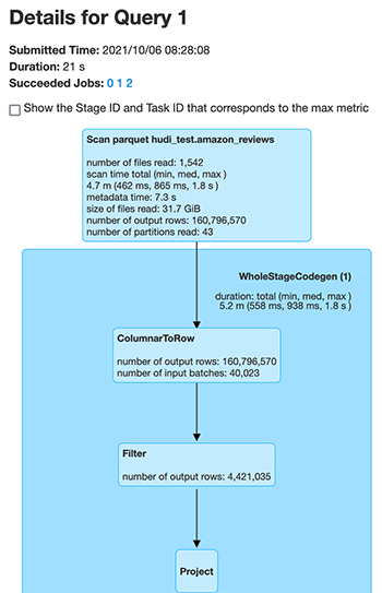
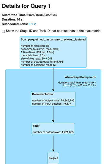
Let’s compare the underlying file scan performance for the two different Hudi tables. The following screenshot is the output from the Spark UI, which shows the changes in the files scanned for the same number of output rows. First we see the files scanned for the unclustered Hudi table.

Next, we see the files scanned for the clustered Hudi table.

The number of files scanned by Spark dropped from 1,542 files for the unclustered Hudi dataset to 85 files for the clustered Hudi dataset for the exact same data. Also, the number of records scanned reduced from 160,796,570 to 78,845,795.

We compared the performance of the preceding query for the amazon_reviews (non-clustered) and amazon_reviews_clustered (clustered) Hudi dataset, across Spark SQL, Hive, and PrestoDB. The cluster configuration used was 1 leader (m5.4xlarge) and 2 cores (m5.4xlarge).

The following chart provides the query performance comparison using different engines for the Hudi table, which are unclustered, and for the Hudi table, which is clustered.

We found that with clustering enabled for the Hudi table, the query performance increased for all three query engines, ranging from 28% to 63%. The following table provides the details for the query performance for the Hudi table, both with clustering enabled and disabled.

Query Engine Non-clustered Table Clustered Table Query Runtime Improvement
Time (in seconds) Time (in seconds)
Spark SQL 21.6 15.4 28.7 %
Hive 96.3 47 51.3 %
PrestoDB 11.7 4.3 63.25 %

Metadata-based file listing

Hudi write operations like compaction, cleaning, and global index, as well as queries, perform a file system listing to get the current view of the partitions and files in the dataset. For small datasets, this shouldn’t impact the performance drastically. However, when working with large data, this listing operation can impact the performance negatively when reading the files. For example, with HDFS as the underlying data store, the list operation for a large number of files or partitions can overwhelm HDFS NameNode and affect the stability of job. In cases where Amazon S3 is used as the underlying data store, O(N) calls for N partitions with a large number of files is time-consuming and can also result in throttling errors.

With Apache Hudi version 0.7.0, you can change this behavior by enabling metadata-based listing for Hudi tables. This partitions and files list is stored in an internal metadata table, which is implemented using a Hudi Merge on Read (MoR) table. This metadata table can take all the advantages of the Hudi MoR table, which includes the capability of low-latency updates, and the ability to atomically commit metadata updates and easily roll back if write fails. It also makes it easy to keep metadata in sync with the Hudi table because both use a timeline for traceability. This index of the file list is stored using HFiles for base and log file format for delta updates. The HFile format allows point-lookups of specific records based on record key. The goal is to reduce O(N) list calls for N partitions to O(1) get call to read the metadata.

We compared query performance for a Hudi dataset with metadata listing enabled vs. not enabled. For this example, we used a larger dataset of 3 TB with Amazon EMR release version 6.3.0. We used the following code snippet to create the metadata enabled and not enabled dataset by setting the HoodieMetadataConfig.METADATA_ENABLE_PROP (hoodie.metadata.enable) config:

val srcPath = "s3://gbrahmi-demo/3-tb-data_store_sales-parquet/"
val tableName = "tpcds_store_sales_3TB_hudi_080"
val tablePath = "s3://emr-hudi-test-data/hudi/hudi_080/" + tableName

val inputDF = spark.read.format("parquet").load(srcPath)

inputDF.write
  .format("hudi")
  .option(HoodieWriteConfig.TABLE_NAME, tableName)
  .option(HoodieMetadataConfig.METADATA_ENABLE_PROP, "true")
  .option(DataSourceWriteOptions.OPERATION_OPT_KEY, DataSourceWriteOptions.BULK_INSERT_OPERATION_OPT_VAL)
  .option(DataSourceWriteOptions.TABLE_TYPE_OPT_KEY, DataSourceWriteOptions.COW_TABLE_TYPE_OPT_VAL)
  .option(DataSourceWriteOptions.RECORDKEY_FIELD_OPT_KEY, "ss_item_sk,ss_ticket_number")
  .option(DataSourceWriteOptions.PARTITIONPATH_FIELD_OPT_KEY, "ss_sold_date_sk")
  .option(DataSourceWriteOptions.PRECOMBINE_FIELD_OPT_KEY, "ss_ticket_number")
  .option(DataSourceWriteOptions.KEYGENERATOR_CLASS_OPT_KEY, "org.apache.hudi.keygen.ComplexKeyGenerator")
  .option(DataSourceWriteOptions.HIVE_SYNC_ENABLED_OPT_KEY, "true")
  .option(DataSourceWriteOptions.HIVE_DATABASE_OPT_KEY, "hudi_test")
  .option(DataSourceWriteOptions.HIVE_TABLE_OPT_KEY, tableName)
 .option(DataSourceWriteOptions.HIVE_PARTITION_FIELDS_OPT_KEY, "ss_sold_date_sk")
.option(DataSourceWriteOptions.HIVE_PARTITION_EXTRACTOR_CLASS_OPT_KEY, "org.apache.hudi.hive.MultiPartKeysValueExtractor")
  .mode(SaveMode.Overwrite)
  .save(tablePath)

On the query engine side, we can enable it via the following methods:

  • Spark data source:
    spark.read.format("hudi")
      .option(HoodieMetadataConfig.METADATA_ENABLE_PROP, "true")
      .load(tablePath + "/*")

  • Spark SQL CLI:
    spark-sql --conf "spark.hadoop.hoodie.metadata.enable=true"
     --jars /usr/lib/hudi/hudi-spark-bundle.jar

  • Hive:
    hive> SET hoodie.metadata.enable = true;

  • PrestoDB:
    presto:default> set session hive.prefer_metadata_to_list_hudi_files=true;

We used the following query to compare query performance via Hive and PrestoDB:

select count(*) from tpcds_store_sales_3TB_hudi_080 where ss_quantity > 50;

The following chart provides the query performance comparison.

We found that with metadata listing, query execution runtime decreased by around 25% for the Hive engine, and by around 32% for PrestoDB. The following table provides the details of query execution runtime with and without metadata listing.

Query Engine Metadata Disabled Metadata Enabled Query Runtime Improvement
Time (in seconds) Time (in seconds)
Hive 415.28533 310.02367 25.35%
Presto 72 48.6 32.50%

Metadata listing considerations

With Hudi 0.7.0 and 0.8.0, you may not observe noticeable improvements for queries via Spark SQL (with metadata listing), because Hudi relies on Spark’s InMemoryFileIndex to do the actual file listing and can’t use the metadata. You may observe improvements because HoodieROPathFilter uses the metadata for its filtering. However, with Hudi release 0.9.0, we’re introducing a custom FileIndex implementation for Hudi to use metadata for file listing instead of relying on Spark. Therefore, from 0.9.0, you will observe noticeable performance improvements for Spark SQL queries.

Amazon CloudWatch integration

Apache Hudi provides MetricsReporter implementations like JmxMetricsReporter, MetricsGraphiteReporter, and DatadogMetricsReporter, which you can use to publish metrics to user-specified sinks. Amazon EMR, with its release 6.4.0 having Hudi 0.8.0, has introduced CloudWatchMetricsReporter, which you can use to publish these metrics to Amazon CloudWatch. It helps publish Hudi writer metrics like commit duration, rollback duration, file-level metrics (number of files added or deleted per commit), record-level metrics (records inserted or updated per commit) and partition-level metrics (partitions inserted or updated per commit). This is useful in debugging Hudi jobs, as well as making decisions around cluster scaling.

You can enable the CloudWatch metric via the following configurations:

hoodie.metrics.on = true
hoodie.metrics.reporter.type = CLOUDWATCH

The following table summarizes additional configurations that you can change if needed.

Configuration Description Value
hoodie.metrics.cloudwatch.report.period.seconds Frequency (in seconds) at which to report metrics to CloudWatch Default value is 60 seconds, which is fine for the default 1-minute resolution offered by CloudWatch
hoodie.metrics.cloudwatch.metric.prefix Prefix to be added to each metric name Default value is empty (no prefix)
hoodie.metrics.cloudwatch.namespace CloudWatch namespace under which metrics are published Default value is Hudi
hoodie.metrics.cloudwatch.maxDatumsPerRequest Maximum number of datums to be included in one request to CloudWatch Default value is 20, which is same as the CloudWatch default

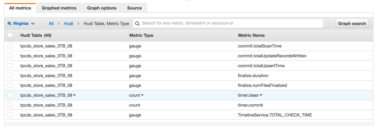
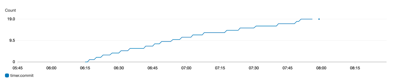
The following screenshot shows some of the metrics published for a particular Hudi table, including the type of metric and its name. These are dropwizard metrics; gauge represents the exact value at a point in time, and counter represents a simple incrementing or decrementing integer.

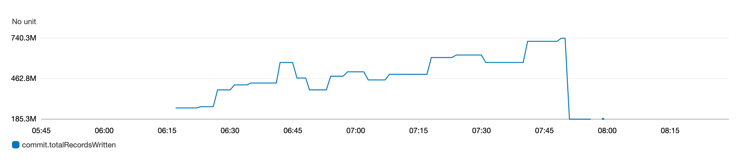
The following graph of the gauge metric represents the total records written to a table over time.

The following graph of the counter metric represents the number of commits increasing over time.

Optimistic Concurrency Control

A major feature that has been introduced with Hudi 0.8.0, and available since Amazon EMR release 6.4.0, is Optimistic Concurrency Control (OCC) to enable multiple writers to concurrently ingest data into the same Hudi table. This is file-level OCC, which means that for any two commits (or writers) happening to the same table at the same time, both are allowed to succeed if they don’t have writes to overlapping files. The feature requires acquiring locks, for which you can use either Zookeeper or HiveMetastore. For more information about the guarantees provided, see Concurrency Control.

Amazon EMR clusters have Zookeeper installed, which you can use as a lock provider to perform concurrent writes from the same cluster. To make it easier to use, Amazon EMR preconfigures the lock provider in the newly introduced /etc/hudi/conf/hudi-defaults.conf file (see the next section) via the following properties:

hoodie.write.lock.provider=org.apache.hudi.client.transaction.lock.ZookeeperBasedLockProvider
hoodie.write.lock.zookeeper.url=<EMR Zookeeper URL>
hoodie.write.lock.zookeeper.port=<EMR Zookeeper Port>
hoodie.write.lock.zookeeper.base_path=/hudi

Although the lock provider is preconfigured, enabling of OCC still needs to be handled by the users either via Hudi job options or at cluster level via the Amazon EMR Configurations API:

hoodie.write.concurrency.mode = optimistic_concurrency_control
hoodie.cleaner.policy.failed.writes = LAZY (Performs cleaning of failed writes lazily instead of inline with every write)
hoodie.write.lock.zookeeper.lock_key = <Key to uniquely identify the Hudi table> (Table Name is a good option)

Amazon EMR configuration support and improvements

Amazon EMR release 6.4.0 has introduced the ability to configure and reconfigure Hudi via the configurations feature. Hudi configurations that are needed across jobs and tables can now be configured at cluster level via the hudi-defaults classification or /etc/hudi/conf/hudi-defaults.conf file, similar to other applications like Spark and Hive. The following code is an example of the hudi-defaults classification to enable metadata-based listing and CloudWatch metrics:

[{
  "Classification": "hudi-defaults",
  "Properties": {
    "hoodie.metadata.enable": "true",
    "hoodie.metadata.insert.parallelism": "3000",
    "hoodie.metrics.on": "true",
    "hoodie.metrics.reporter.type": "CLOUDWATCH"
  }
}]

Amazon EMR automatically configures suitable defaults for a few configs, to improve the user experience by removing the need for customers having to pass them:

  • HIVE_URL_OPT_KEY is configured to the cluster’s Hive server URL and no longer needs to be specified. This is particularly useful when running a job in Spark cluster mode, where users previously had to determine and themselves specify the Amazon EMR primary IP.
  • HBase specific configurations, which are useful for using HBase index with Hudi.
  • Zookeeper lock provider specific configuration, as discussed under concurrency control, which makes it easier to use OCC.

Additional changes have been introduced to reduce the number of configurations that users need to pass, and to infer automatically where possible:

Apache Flink integration

Apache Hudi started off with a very tight integration with Apache Spark. With release version 0.7.0, we now have integrations available to ingest data using Apache Flink. It required decoupling Spark from the internal table format, writers, and table services code in a way that can be used by other evolving engines in the industry like Flink.

Hudi 0.7.0 provides initial Flink support via HooodieFlinkStreamer, which you can use to write CoW tables by streaming data from a Kafka topic using Apache Flink. For example, you can use the following Flink command to start reading the topic ExampleTopic from the Kafka brokers broker-1, broker-2, and broker-3 running on port 9092:

./bin/flink run -c org.apache.hudi.HoodieFlinkStreamer \
  -m yarn-cluster -d -yjm 1024 -ytm 1024 -p 4 -ys 3 \
  -ynm hudi_on_flink_example \
  /usr/lib/hudi/hudi-flink-bundle.jar \
  --kafka-topic ExampleTopic \
  --kafka-group-id <kafka-group-id> \
  --kafka-bootstrap-servers broker-1:9092,broker-2:9092,broker-3:9092 \
  --table-type COPY_ON_WRITE \
  --target-table hudi_flink_table \
  --target-base-path s3://emr-hudi-test-data/hudi/hudi_070/hudi_flink_table \
  --props hdfs:///hudi/flink/config/hudi-jobConf.properties \
  --checkpoint-interval 6000 \
  --flink-checkpoint-path hdfs:///hudi/hudi-flink-checkpoint-dir

With Hudi 0.8.0, there have been major improvements in Flink integration performance and scalability, as well as the introduction of new features like SQL connector for both source and sink, writer for MoR, batch reader for CoW and MoR, streaming reader for MoR, and state-backed indexing with bootstrap support. For more information about Flink integration design, see Apache Hudi meets Apache Flink. To get started with Flink SQL, see Flink Guide.

Kafka commit callbacks

The previous version (0.6.0) of Apache Hudi introduced write commit callback functionality. With this functionality, Hudi can send a callback message every time a successful commit arrives to the Hudi dataset. The write commit callback supported HTTP method in the previous release. With Apache Hudi release version 0.7.0, Hudi now supports write commit callback for Kafka as well. Using Kafka for sending the callback messages for every successful commit can now enable you to build asynchronous data pipelines or business processing logic every time the Hudi dataset sees a new commit. You can now build incremental ETL pipelines for processing new events that arrive in the Hudi data lake.

The implementation of Kafka commit callback uses HoodieWriteCommitKafkaCallback as the hoodie.write.commit.callback.class. Besides setting the commit callback class, you can also set up additional parameters for the Kafka bootstrap servers and the topic configurations.

The following is a code snippet where commit callback messages are published to the Kafka topic ExampleTopic hosted on the Kafka brokers b-1.demo-hudi.xxxxxx.xxx.kafka.us-east-1.amazonaws.com, b-2.demo-hudi.xxxxxx.xxx.kafka.us-east-1.amazonaws.com, and b-3.demo-hudi.xxxxxx.xxx.kafka.us-east-1.amazonaws.com when writing to a Hudi dataset:

import org.apache.hudi.QuickstartUtils._
import scala.collection.JavaConversions._
import org.apache.spark.sql.SaveMode._
import org.apache.hudi.DataSourceReadOptions._
import org.apache.hudi.DataSourceWriteOptions._
import org.apache.hudi.config.HoodieWriteConfig._
 
val tableName = "trips_data_kafka_callback"
val tablePath = "s3://gbrahmi-sample-bucket/hudi-dataset/hudi_kafka_callback/" + tableName
 
val dataGen = new DataGenerator(Array("2021/05/01"))
val updates = convertToStringList(dataGen.generateInserts(10))
 
val df = spark.read.json(spark.sparkContext.parallelize(updates, 1))
 
df.write.format("hudi").
  option(TABLE_NAME, tableName).
  option(PRECOMBINE_FIELD_OPT_KEY, "ts").
  option(RECORDKEY_FIELD_OPT_KEY, "uuid").
  option("hoodie.write.commit.callback.on", "true").
  option("hoodie.write.commit.callback.class", "org.apache.hudi.utilities.callback.kafka.HoodieWriteCommitKafkaCallback").
  option("hoodie.write.commit.callback.kafka.bootstrap.servers", "b-1.demo-hudi.xxxxxx.xxx.kafka.us-east-1.amazonaws.com:9092,b-2.demo-hudi.xxxxxx.xxx.kafka.us-east-1.amazonaws.com:9092,b-3.demo-hudi.xxxxxx.xxx.kafka.us-east-1.amazonaws.com:9092").
  option("hoodie.write.commit.callback.kafka.topic", "ExampleTopic").
  option("hoodie.write.commit.callback.kafka.acks", "all").
  option("hoodie.write.commit.callback.kafka.retries", 3).
  mode(Append).
  save(tablePath)

The following is how the messages appear in your Kafka topic:

{"commitTime":"20210508210230","tableName":"trips_data_kafka_callback","basePath":"s3:// gbrahmi-sample-bucket/hudi-dataset/hudi_kafka_callback/trips_data_kafka_callback"}

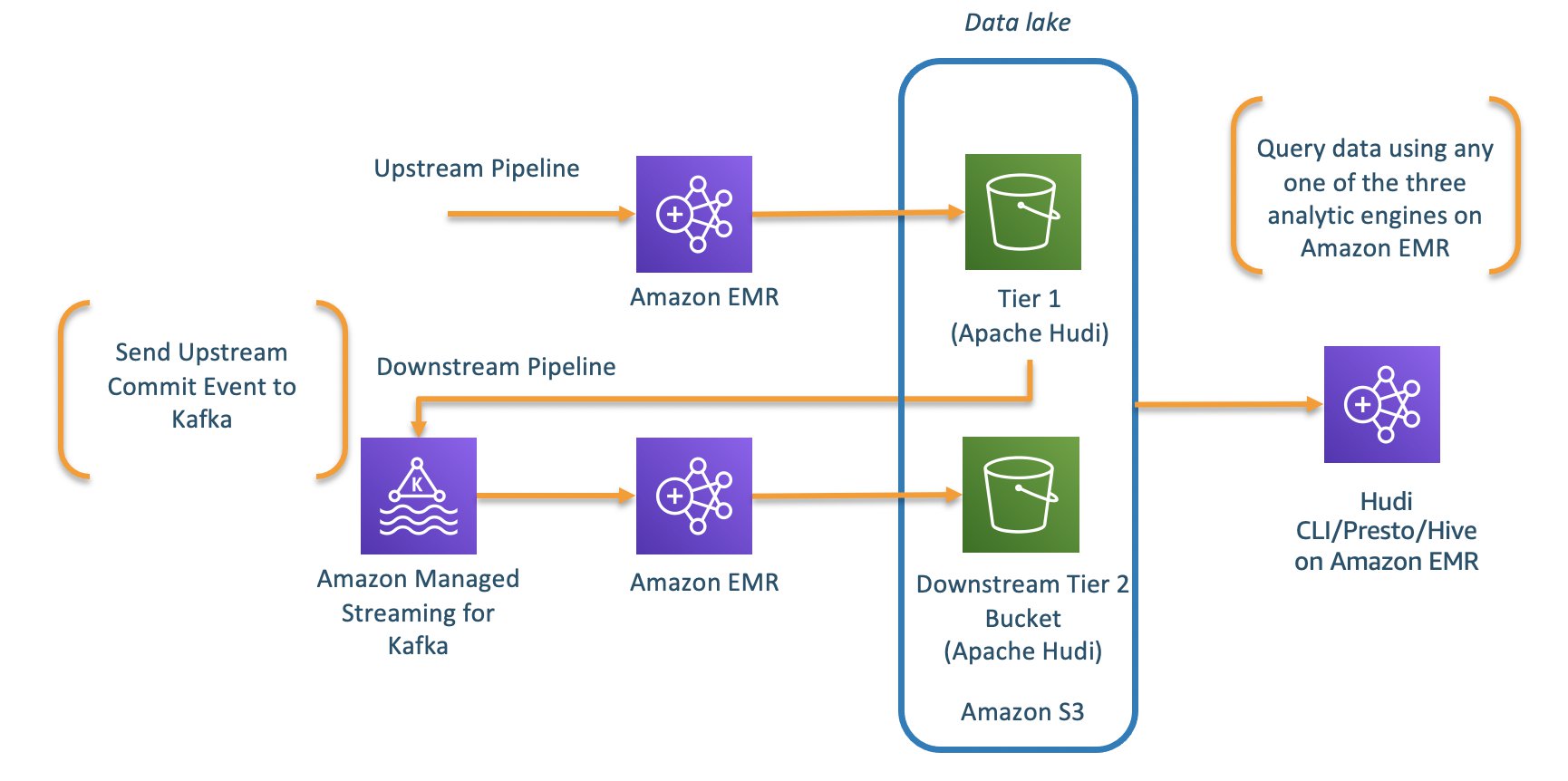
A downstream pipeline can now easily query these events from Kafka and process the incremental data into derived Hudi tables.

Other improvements

Besides the aforementioned improvements, there have been some additional changes worth mentioning. On the writer side, there are the following improvements:

  • Support for Spark 3 – Support for writing and querying the data using Apache Spark 3 is now available with Apache Hudi 0.7.0 onwards. This works with Scala 2.12 bundle for hudi-spark-bundle.
  • Insert overwrite and insert overwrite table write operations – Apache Hudi 0.7.0 introduces two new operations, insert_overwrite and insert_overwrite_table, to support batch ETL jobs where an entire table or partition is overwritten during each execution. You can use these operations instead of the upsert operation, and it’s must cheaper to run.
  • Delete partitions – The new API is now available since 0.7.0 to delete an entire partition. This helps avoid the use of record-level deletes.
  • Java writer support – Hudi 0.7.0 introduced Java-based writing support via the HoodieJavaWriteClient class.

Similarly, on the query integration side, there have been the following improvements:

  • Structured streaming reads – Hudi 0.8.0 introduced a Spark structured streaming source implementation via the HoodieStreamSource class. You can use it to support streaming reads from Hudi tables.
  • Incremental query on MoR – Since Hudi 0.7.0, we now have incremental query support for MoR tables, which you can use to incrementally pull data by downstream applications.

Conclusion

The new features introduced in Apachi Hudi enable you to build decoupled solutions by using features like Kafka commit callback and Flink integration with Apache Hudi with Amazon EMR. You can also improve your overall performance of the Hudi data lake by using the capabilities of clustering and metadata tables.


About the Authors

Udit Mehrotra is a software development engineer at Amazon Web Services and an Apache Hudi PMC member/committer. He works on cutting-edge features of Amazon EMR and is also involved in open-source projects such as Apache Hudi, Apache Spark, Apache Hadoop, and Apache Hive. In his spare time, he likes to play guitar, travel, binge watch, and hang out with friends.

Gagan Brahmi is a Specialist Solutions Architect focused on Big Data & Analytics at Amazon Web Services. Gagan has over 16 years of experience in information technology. He helps customers architect and build highly scalable, performant, and secure cloud-based solutions on AWS.

The collective thoughts of the interwebz