Post Syndicated from Kaituo Li original https://aws.amazon.com/blogs/big-data/detect-anomalies-on-one-million-unique-entities-with-amazon-opensearch-service/
Amazon OpenSearch Service (successor to Amazon Elasticsearch Service) supports a highly performant, integrated anomaly detection engine that enables the real-time identification of anomalies in streaming data. Last year, we released high-cardinality anomaly detection (HCAD) to detect individual entities’ anomalies. With the 1.1 release, we have allowed you to monitor a million entities with steady, predictable performance. HCAD is easiest when described in contrast to the non-HCAD single-stream solution. In a single-stream detector, we detect anomalies for an aggregate entity. For example, we can use a single-stream detector to sift through aggregated traffic across all IP addresses so that users can be notified when unusual spikes occur. However, we often need to identify anomalies in entities, such as individual hosts and IP addresses. Each entity may work on a different baseline, which means its time series’ distribution (measured in parameters such as magnitude, trend, and seasonality, to name a few) are different. The different baselines make it inaccurate to detect anomalies using a single monolithic model. HCAD distinguishes itself from single-stream detectors by customizing anomaly detection models to entities.
Example use cases of HCAD include the following:
- Internet of things – Continuously tracking the temperature of fridges and warning users of temperatures at which food or medicine longevity is at risk, so users can take measures to avoid them. Each entity has specific categorical fields that describe it, and you can think of the categorical fields as characteristics for those entities. A fridge’s serial number is the categorical field that uniquely identifies the fridges. Using a single model generates a lot of false alarms because ambient temperatures can be different. A temperature of 5° C is normal during winter in Seattle, US, but such a temperature in a tropical place during winter is likely anomalous. Also, users may open the door to a fridge several times, triggering a spike in the temperature. The duration and frequency of spikes can vary according to user behavior. HCAD can group temperature data into geographies and users to detect varying local temperatures and user behavior.
- Security – An intrusion detection system identifying an increase in failed login attempts in authentication logs. The user name and host IP are the categorical fields used to determine the user accessing from the host. Hackers might guess user passwords by brute force, and not all users on the same host IP may be targeted. The number of failed login counts varies on a host for a particular user at a specific time of day. HCAD creates a representative baseline per user on each host and adapts to changes in the baseline.
- IT operations – Monitoring access traffic by shard in a distributed service. The shard ID is the categorical field, and the entity is the shard. A modern distributed system usually consists of shards linked together. When a shard experiences an outage, the traffic increases significantly for dependent shards due to retry storms. It’s hard to discover the increase because only a limited number of shards are affected. For example, traffic on the related shards might be as much as 64 times that of normal levels, whereas average traffic across all shards might just grow by a small constant factor (less than 2).
Making HCAD real time and performant while achieving completeness and scalability is a formidable challenge:
- Completeness – Model all or as many entities as possible.
- Scalability – Horizontal and vertical scaling without changing model fidelity. That is, when scaling the machine up or out, an anomaly detector can add models monotonically. HCAD uses the same model and gives the same answer for an entity’s time series as in single-stream detection.
- Performance – Low impact to system resource usage and high overall throughput.
The first release of HCAD in Amazon OpenSearch Service traded completeness and scalability for performance: the anomaly detector limited the number of entities to 1,000. You can change the setting plugins.anomaly_detection.max_entities_per_query to increase the number of monitored entities per interval. However, such a change incurs a non-negligible cost, which opens the door to cluster instability. Each entity uses memory to host models, disk I/O to read and write model checkpoints and anomaly results, CPU cycles for metadata maintenance and model training and inference, and garbage collection for deleted models and metadata. The more entities, the more resource usage. Furthermore, HCAD could suffer a combinatorial explosion of entities when supporting multiple categorical fields (a feature released in Amazon OpenSearch Service 1.1). Imagine a detector with only one categorical field geolocation. Geolocation has 1,000 possible values. Adding another categorical field product with 1,000 allowed values gives the detector 1 million entities.
For the next version of HCAD, we devoted much effort to improving completeness and scalability. Our approach captures sizing a cluster right and combines in-memory model hosting and on-disk model loading. Performance metrics show HCAD doesn’t saturate the cluster with substantial cost and still leaves plenty of room for other tasks. As a result, HCAD can analyze one million entities in 10 minutes and flags anomalies in different patterns. In this post, we will explore how HCAD can analyze one million entities and the technical implementations behind the improvements.
How to size domains
Model management is a trade-off: disk-based solutions that reload-use-stop-store models on every interval offer savings in memory but suffer high overhead and are hard to scale. Memory-based solutions offer lower overhead and higher throughput but typically increase memory requirements. We exploit the trade-off by implementing an adaptive mechanism that hosts models in memory as much as allowed (capped via the cluster setting plugins.anomaly_detection.model_max_size_percent), as required by best performance. When models don’t fit in memory, we process extra model requests by loading models from disks.
The use of memory whenever possible is responsible for the HCAD scalability. Therefore, it is crucial to sizing a cluster right to offer enough memory for HCAD. The main factors to consider when sizing a cluster are:
- Sum of all detectors’ total entity count – A detector’s total entity count is the cardinality of the categorical fields. If there are multiple categorical fields, the number counts all unique combinations of values of these fields present in data. You can decide the cardinality via cardinality aggregation in Amazon OpenSearch Service. If the detector is a single-stream detector, the number of entities is one because there is no defined categorical field.
- Heap size – Amazon OpenSearch Service sets aside 50% of RAM for heap. To determine the heap size of an instance type, refer to Amazon OpenSearch Service pricing. For example, an r5.2xlarge host has 64 GB RAM. Therefore, the host’s heap size is 32 GB.
- Anomaly detection (AD) maximum memory percentage – AD can use up to 10% of the heap by default. You can customize the percentage via the cluster setting
plugins.anomaly_detection.model_max_size_percent. The following update allows AD to use half of the heap via the aforementioned setting:
PUT /_cluster/settings
{
	"persistent": {
		"plugins.anomaly_detection.model_max_size_percent": "0.5"
	}
}
- Entity in-memory model size – An entity’s in-memory model size varies according to shingle size, the number of features, and Amazon OpenSearch Service version as we’re constantly improving. All entity models of the same detector configuration in the same software version have the same size. A safe way to obtain the size is to run a profile API on the same detector configuration on an experimental cluster before creating a production cluster. In the following case, each entity model of detector fkzfBX0BHok1ZbMqLMdu is of size 470,491 bytes:
Enter the following profile request:
GET /_plugins/_anomaly_detection/detectors/fkzfBX0BHok1ZbMqLMdu/_profile/models
We get the following response:
{
	...{
		"model_id": "fkzfBX0BHok1ZbMqLMdu_entity_GOIubzeHCXV-k6y_AA4K3Q",
		"entity": [{
				"name": "host",
				"value": "host141"
			},
			{
				"name": "process",
				"value": "process54"
			}
		],
		"model_size_in_bytes": 470491,
		"node_id": "OcxBDJKYRYKwCLDtWUKItQ"
	}
	...
}
- Storage requirement for result indexes – Real-time detectors store detection results as much as possible when the indexing pressure isn’t high, including both anomalous and non-anomalous results. When the indexing pressure is high, we save anomalous and a random subset of non-anomalous results. OpenSearch Dashboard employs non-anomalous results as the context of abnormal results and plots the results as a function of time. Additionally, AD stores the history of all generated results for a configurable number of days after generating results. This result retention period is 30 days by default, and adjustable via the cluster setting
plugins.anomaly_detection.ad_result_history_retention_period. We need to ensure enough disk space is available to store the results by multiplying the amount of data generated per day by the retention period. For example, consider a detector that generates 1 million result documents for a 10-minute interval detector with 1 million entities per interval. One document’s size is about 1 KB. That’s roughly 144 GB per day, 4,320 GB after a 30-day retention period. The total disk requirement should also be multiplied by the number of shard copies. Currently, AD chooses one primary shard per node (up to 10) and one replica when called for the first time. Because the number of replicas is 1, every shard has two copies, and the total disk requirement is closer to 8,640 GB for the million entities in our example.
- Anomaly detection overhead – AD incurs memory overhead for historical analyses and internal operations. We recommend reserving 20% more memory for the overhead to keep running models uninterrupted.
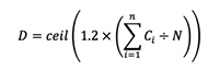
In order to derive the required number of data nodes D, we must first derive an expression for the number of entity models N that a node can host in memory. We define Si to be the entity model size of detector i. If we use an instance type with heap size H where the maximum AD memory percentage is P, N is equal to AD memory allowance divided by the maximum entity model size among all detectors:

We consider the required number of data nodes D as a function of N. Let’s denote by Ci the total entity counts of detector i. Given n detectors, it follows that:

The fact that AD needs an extra 20% memory overhead is expressed by multiplying 1.2 in the formula. The ceil function represents the smallest integer greater than or equal to the argument.
For example, an r5.2xlarge Amazon Elastic Compute Cloud (Amazon EC2) instance has 64 GB RAM, so the heap size is 32 GB. We configure AD to use at most half of the allowed heap size. We have two HCAD detectors, whose model sizes are 471 KB and 403 KB, respectively. To host 500,000 entities for each detector, we need a 36-data-node cluster according to the following calculation:

We also need to ensure there is enough disk space. In the end, we used a 39-node r5.2xlarge cluster (3 primary and 36 data nodes) with 4 TB Amazon Elastic Block Store (EBS) storage on each node.
What if a detector’s entity count is unknown?
Sometimes, it’s hard to know a detector’s entity count. We can check historical data and estimate the cardinality. But it’s impossible to predict the future accurately. A general guideline is to allocate buffer memory during planning. Appropriately used, buffer memory provides room for small changes. If the changes are significant, you can adjust the number of data nodes because HCAD can scale in and out horizontally.
What if the number of active entities is changing?
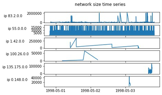
The total number of entities created can be higher than the number of active entities, as evident from the following two figures. The total number of entities in the HTTP logs dataset is 2 million within 2 months, but each entity only appears seven times on average. The number of active entities within a time-boxed interval is much less than 2 million. The following figure presents an example time series of network size of IP addresses from the HTTP logs dataset.

The KPI dataset also shows similar behavior, where entities often appear in a short amount of time during bursts of entity activities.

AD requires large sample sizes to create a comprehensive picture of the data patterns, making it suitable for dense time series that can be uniformly sampled. AD can still train models and produce predictions if the preceding bursty behavior can last a while and provide at least 400 points. However, training becomes more difficult, and prediction accuracy is lower as data gets more sparse.
It’s wasteful to preallocate memory according to the total number of entities in this case. Instead of the total number of entities, we need to consider the maximal active entities within an interval. You can get an approximate number by using a date_histogram and cardinality aggregation pipeline, and sorting during a representative period. You can run the following query if you’re indexing host-cloudwatch and want to find out the maximal number of active hosts within a 10-minute interval throughout 10 days:
GET /host-cloudwatch/_search?size=0
{
	"query": {
		"range": {
			"@timestamp": {
				"gte": "2021-11-17T22:21:48",
				"lte": "2021-11-27T22:22:48"
			}
		}
	},
	"aggs": {
		"by_10m": {
			"date_histogram": {
				"field": "@timestamp",
				"fixed_interval": "10m"
			},
			"aggs": {
				"dimension": {
					"cardinality": {
						"field": "host"
					}
				},
				"multi_buckets_sort": {
					"bucket_sort": {
						"sort": [{
							"dimension": {
								"order": "desc"
							}
						}],
						"size": 1
					}
				}
			}
		}
	}
}
The query result shows that at most about 1,000 hosts are active during a ten-minute interval:
{
	...
	"aggregations": {
		"by_10m": {
			"buckets": [{
				"key_as_string": "2021-11-17T22:30:00.000Z",
				"key": 1637188200000,
				"doc_count": 1000000,
				"dimension": {
					"value": 1000
				}
			}]
		}
	}
	...
}
HCAD has a cache to store models and maintain a timestamp of last access for each model. For each model, an hourly job checks the time of inactivity and invalidates the model if the time of inactivity is longer than 1 hour. Depending on the timing of the hourly check and the cache capacity, the elapsed time a model is cached varies. If the cache capacity isn’t large enough to hold all non-expired models, we have an adapted least frequently used (LFU) cache policy to evict models (more on this in a later section), and the cache time of those invalidated models is less than 1 hour. If the last access time of a model is reset immediately after the hourly check, when the next hourly check happens, the model doesn’t expire. The model can take another hour to expire when the next hourly check comes. So the max cache time is 2 hours.
The upper bound of active entities that detector i can observe is:

This equation has the following parameters:
- Ai is the maximum number of active entities per interval of detector i. We get the number from the preceding query.
- 120 is the number of minutes in 2 hours. ∆Ti denotes detector i’s interval in minutes. The ceil function represents the smallest integer greater than or equal the argument. ceil(120÷∆Ti) refers to the max number of intervals a model is cached.
Accordingly, we should account for Bi in the sizing formula:

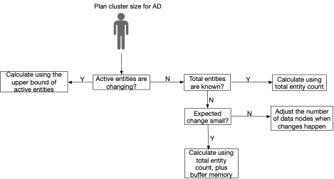
Sizing calculation flow chart
With the definitions of calculating the number of data nodes in place, we can use the following flow chart to make decisions under different scenarios.

What if the cluster is underscaled?
If the cluster is underscaled, AD prioritizes more frequent and recent entities. AD makes its best effort to accommodate extra entities by loading their models on demand from disk without hosting them in the in-memory cache. Loading the models on demand means reloading-using-stopping-storing models at every interval, whose overheads are quite high. The overheads mostly have to do with network or disk I/O, rather than with the cost of model inferencing. Therefore, we did it in a steady, controlled manner. If the system resource usage isn’t heavy and there is enough time, HCAD may finish processing the extra entities. Otherwise, HCAD doesn’t necessarily find all the anomalies it could otherwise find.
Example: Analysis of 1 million entities
In the following example, you will learn how to set up a detector to analyze one million entities.
Ingest data
We generated 10 billion documents for 1 million entities in our evaluation of scalability and completeness improvement. Each entity has a cosine wave time series with randomly injected anomalies. With help from the tips in this post, we created the index host-cloudwatch and ingested the documents into the cluster. host-cloudwatch records elapsed CPU and JVM garbage collection (GC) time by a process within a host. Index mapping is as follows:
{
	...
	"mappings": {
		"properties": {
			"@timestamp": {
				"type": "date"
			},
			"cpuTime": {
				"type": "double"
			},
			"jvmGcTime": {
				"type": "double"
			},
			"host": {
				"type": "keyword"
			},
			"process": {
				"type": "keyword"
			}
		}
	}
	...
}
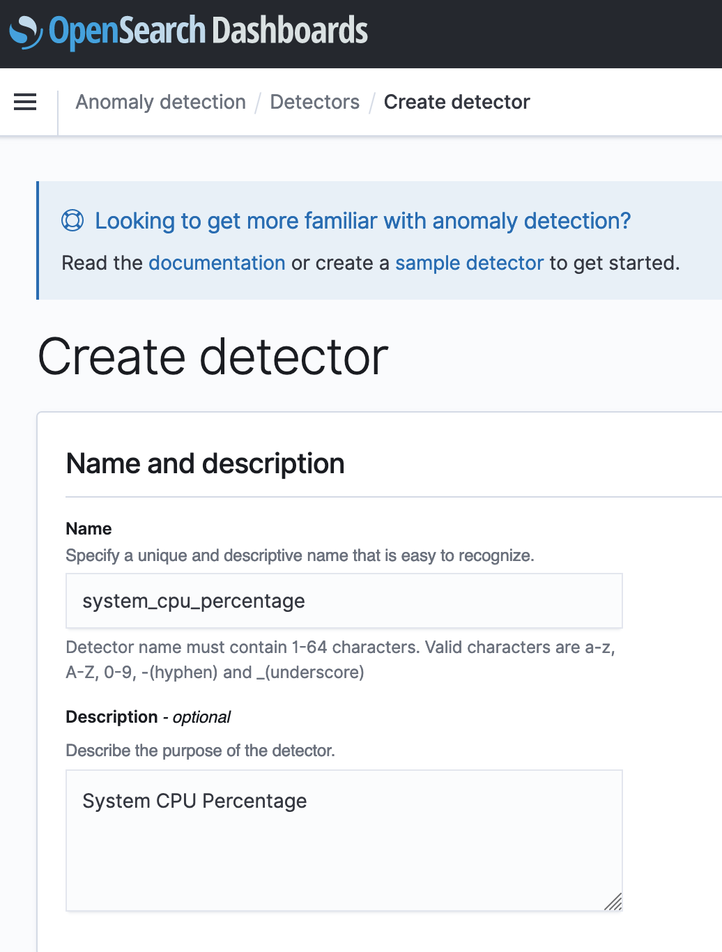
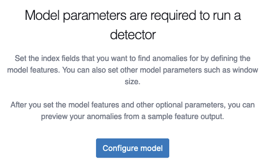
Create a detector
Consider the following factors before you create a detector:
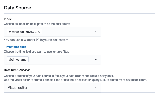
- Indexes to monitor – You can use a group of index names, aliases, or patterns. Here we use the host-cloudwatch index created in the last step.
- Timestamp field – A detector monitors time series data. Each document in the provided index must be associated with a timestamp. In our example, we use the @timetamp field.
- Filter – A filter selects data you want to analyze based on some condition. One example filter selects requests with status code 400 afterwards from HTTP request logs. The 4xx and 5xx classes of HTTP status code indicate that a request is returned with an error. Then you can create an anomaly detector for the number of error requests. In our running example, we analyze all of the data, and thus no filter is used.
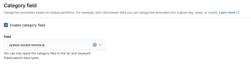
- Category field – Every entity has specific characteristics that describe it. Category fields provide categories of those characteristics. An entity can have up to two category fields as of Amazon OpenSearch Service 1.1. Here we monitor a specific process of a particular host by specifying the process and host field.
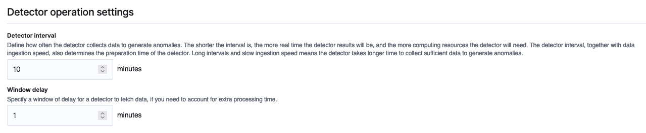
- Detector interval – The detector interval is typically application-defined. We aggregate data within an interval and run models on the aggregated data. As mentioned earlier, AD is suitable for dense time series that can be uniformly sampled. You should at least make sure most intervals have data. Also, different detector intervals require different trade-offs between delay and accuracy. Long intervals smooth out long-term and short-term workload fluctuations and, therefore, may be less prone to noise, resulting in a high delay in detection. Short intervals lead to quicker detection but may find anticipated workload fluctuations instead of anomalies. You can plot your time series with various intervals and observe which interval keeps relevant anomalies while reducing noise. For this example, we use the default 10-minute interval.
- Feature – A feature is an aggregated value extracted from the monitored data. It gets sent to models to measure the degrees of abnormality. Forming a feature can be as simple as picking a field to monitor and the aggregation function that summarizes the field data as metrics. We provide a suite of functions such as min and average. You can also use a runtime field via scripting. We’re interested in the garbage collection time field aggregated via the average function in this example.
- Window delay – Ingestion delay. If the value isn’t configured correctly, a detector might analyze data before the late data arrives at the cluster. Because we ingested all the data in advance, the window delay is 0 in this case.
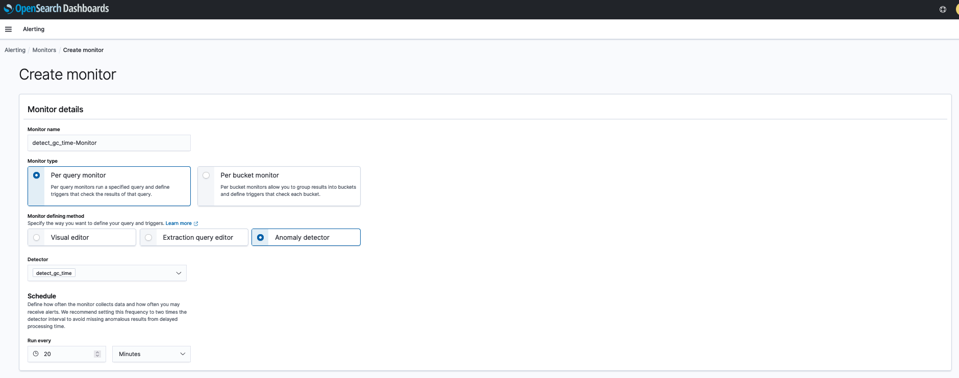
Our detector’s configuration aggregates average garbage collection processing time every 10 minutes and analyzes the average at the granularity of processes on different hosts. The API request to create such a detector is as follows. You can also use our streamlined UI to create and start a detector.
POST _plugins/_anomaly_detection/detectors
{
	"name": "detect_gc_time",
	"description": "detect gc processing time anomaly",
	"time_field": "@timestamp",
	"indices": [
		"host-cloudwatch"
	],
	"category_field": ["host", "process"],
	"feature_attributes": [{
		"feature_name": "jvmGcTime average",
		"feature_enabled": true,
		"importance": 1,
		"aggregation_query": {
			"gc_time_average": {
				"avg": {
					"field": "jvmGcTime"
				}
			}
		}
	}],
	"detection_interval": {
		"period": {
			"interval": 10,
			"unit": "MINUTES"
		}
	},
	"schema_version": 2
}
After the initial training is complete, all models of the 1 million entities are up in the memory, and 1 million results are generated every detector interval after a few hours. To verify the number of active models in the cache, you can run the profile API:
GET /_plugins/_anomaly_detection/detectors/fkzfBX0BHok1ZbMqLMdu/_profile/models
We get the following response:
{
	...
	"model_count": 1000000
}
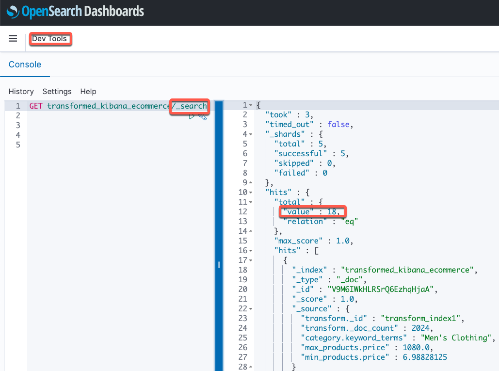
You can observe how many results are generated every detector interval (in our case 10 minutes) by invoking the result search API:
GET /_plugins/_anomaly_detection/detectors/results/_search
{
	"query": {
		"range": {
			"execution_start_time": {
				"gte": 1636501467000,
				"lte": 1636502067000
			}
		}
	},
	"track_total_hits": true
}
We get the following response:
{
	...
	"hits": {
		"total": {
			"value": 1000000,
			"relation": "eq"
		},
		...
	}
	...
}
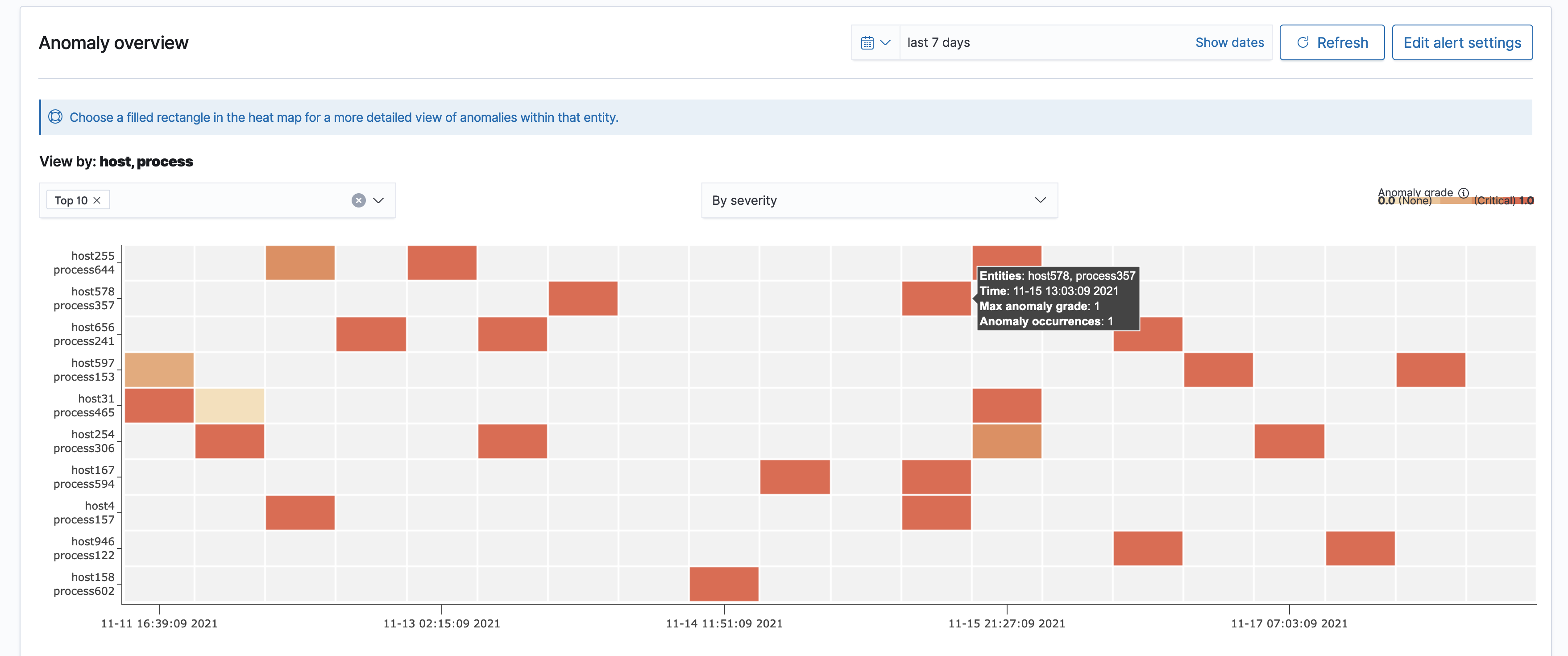
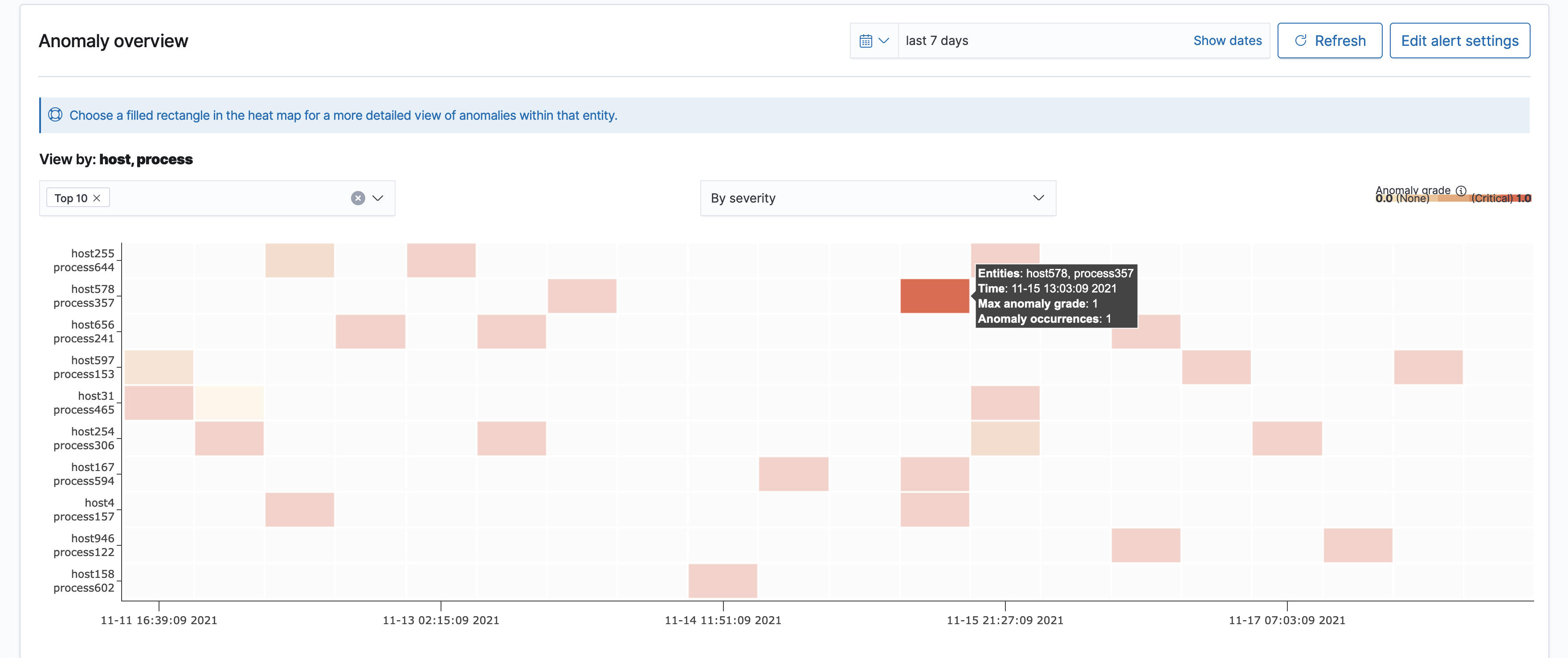
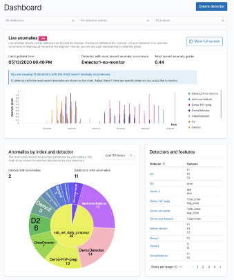
The OpenSearch Dashboard gives an exposition of the top entities producing the most severe or most number of anomalies.

You can choose a colored cell to review the details of anomalies occurring within that given period.

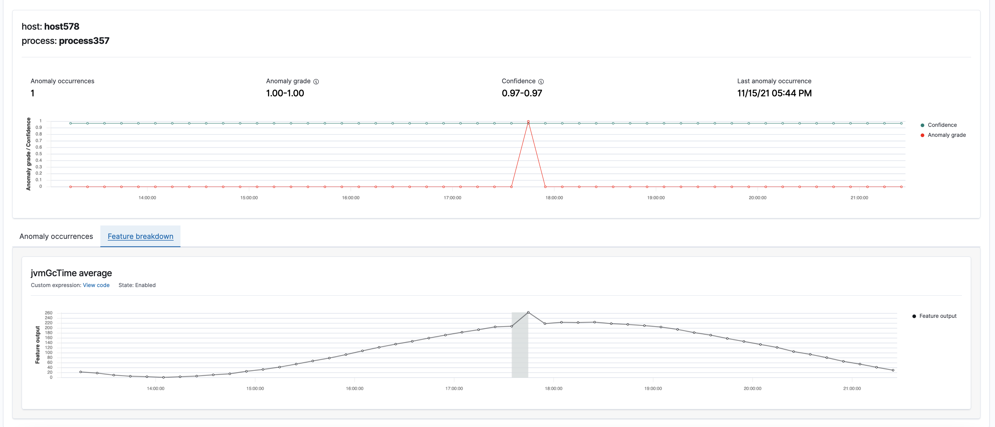
You can view anomaly grade, confidence, and the corresponding features in a shaded area.

Create a monitor
You can create an alerting monitor to notify you of anomalies based on the defined anomaly detector, as shown in the following screenshot.

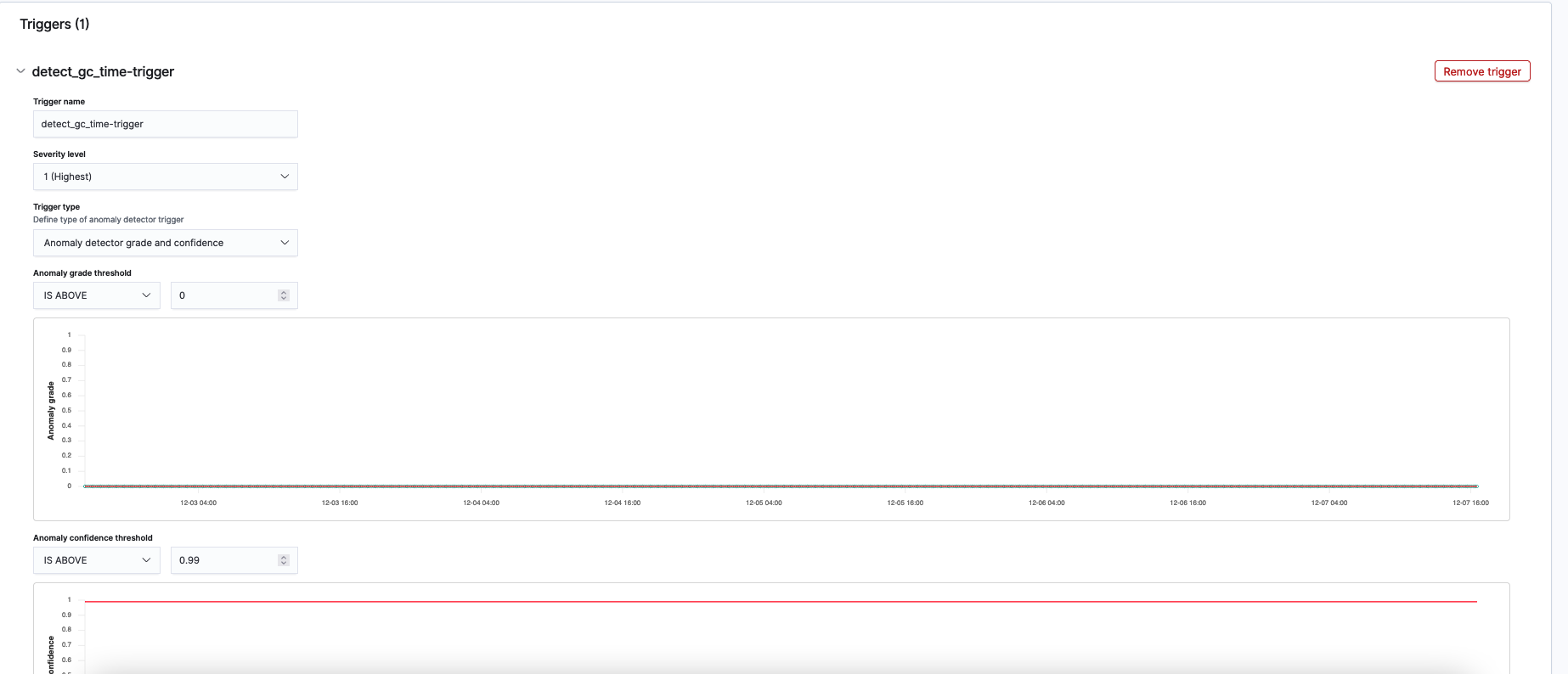
We use anomaly grade and confidence to define a trigger. Both anomaly grade and confidence are values between 0 and 1.
Anomaly grade represents the severity of an anomaly. The closer the grade is to 1, the higher the severity. 0 grade means the corresponding prediction isn’t an anomaly.
Confidence measures whether an entity’s model has observed enough data such that the model contains enough unique, real-world data points. If a confidence value from one model is larger than the confidence of a different model, then the anomaly from the first model has observed more data.
Because we want to receive high fidelity alerts, we configured the grade threshold to be 0 and the confidence threshold to be 0.99.

The final step of creating a monitor is to add an action on what to include in the notification. Our example detector finds anomalies at a particular process in a host. The notification message should contain the entity identity. In this example, we use ctx.results.0.hits.hits.0._source.entity to grab the entity identity.

A monitor based on a detector extracts the maximum grade anomaly and triggers an alert based on the configured grade and confidence threshold. The following is an example alert message:
Attention

Monitor detect_cpu_gc_time2-Monitor just entered alert status. Please investigate the issue.
- Trigger: detect_cpu_gc_time2-trigger
- Severity: 1
- Period start: 2021-12-08T01:01:15.919Z
- Period end: 2021-12-08T01:21:15.919Z
- Entity: {0={name=host, value=host107}, 1={name=process, value=process622}}
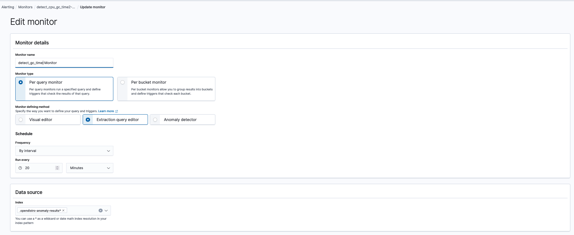
You can customize the extraction query and trigger condition by changing the monitor defining method to Extraction query monitor and modifying the corresponding query and condition. Here is the explanation of all anomaly result index fields you can query.

Evaluation
In this section, we evaluate HCAD’s precision, recall, and overall performance.
Precision and recall
We evaluated precision and recall over the cosine wave data, as mentioned earlier. Such evaluations aren’t easy in the context of real-time processing because only one point is available per entity during each detector interval (10 minutes in the example). Processing all the points takes a long time. Instead, we simulated real-time processing by fast-forwarding the processing in a script. The results are an average of 100 runs. The standard deviation is around 0.12.
The overall average precision, including the effects of cold start using linear interpolation, for the synthetic data is 0.57. The recall is 0.61. We note that no transformations were applied; it’s possible and likely that transformations improve these numbers. The precision is 0.09, and recall is 0.34 for the first 300 points due to interpolated cold start data for training. The numbers pick up as the model observes more real data. After another 5,000 real data points, the precision and recall improve to 0.57 and 0.63, respectively. We reiterate that the exact numbers vary based on the data characteristics—a different benchmark or detection configuration would have other numbers. Further, if there is no missing data, the fidelity of the HCAD model would be the same as that of a single-stream detector.
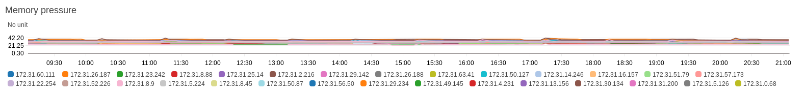
Performance
We ran HCAD on an idle cluster without ingestion or search traffic. Metrics such as JVM memory pressure and CPU of each node are well within the safe zone, as shown in the following screenshot. JVM memory pressure varies between 23–39%. CPU is mostly around 1%, with hourly spikes up to 65%. An internal hourly maintenance job can account for the spike due to saving hundreds of thousands of model checkpoints, clearing unused models, and performing bookkeeping for internal states. However, this can be a future improvement.

Implementation
We next discuss the specifics of the technical work that is germane to HCAD’s completeness and scalability.
RCF 2.0
In Amazon OpenSearch Service 1.1, we integrated with Random Cut Forest library (RCF) 2.0. RCF is based on partitioning data into different bounding boxes. The previous RCF version maintains bounding boxes in memory. However, a real-time detector only uses the bounding boxes when processing a new data point and leaves them dormant most of the time. RCF 2.0 allows for recreating those bounding boxes when required so that bounding boxes are present in memory when processing the corresponding input. The on-demand recreation has led to nine times memory overhead reduction and therefore can support hosting nine times as many models in a node. In addition, RCF 2.0 revamps the serialization module. The new module serializes and deserializes a model 26 times faster using 20 times smaller disk space.
Pagination
Regarding feature aggregation, we switched from getting top hits using terms aggregation to pagination via composite aggregation. We evaluated multiple pagination implementations using a generated dataset with 1 million entities. Each entity has two documents. The experiment configurations can vary according to the number of data nodes, primary shards, and categorical fields. We believe composite queries are the right choice because even though they may not be the fastest in all cases, they’re the most stable on average (40 seconds).
Amortize expensive operations
HCAD can face thundering herd traffic, in which many entities make requests like reading checkpoints from disks at approximately the same time. Therefore, we create various queues to buffer pent-up requests. These queues amortize expensive costs by performing a small and bounded amount of work steadily. Therefore, HCAD can offer predictable performance and availability at scale.
In-memory cache
HCAD appeals to caching to process entities whose memory requirement is larger than the configured memory size. At first, we tried a least recently used cache but experienced thrashing when running the HTTP logs workload: with 100 1-minute interval detectors and millions of entities for each detector, we saw few cache hits (many hundreds) within 7 hours. We were wasting CPU cycles swapping models in and out of memory all the time. As a general rule, a hit-to-miss ratio worse than 3:1 is not worth considering caching for quick model accesses.
Instead, we turned to a modified LFU caching, augmented to include heavy hitters’ approximation. A decayed count is maintained for each model in the cache. The decayed count for a model in the cache is incremented when the model is accessed. The model with the smallest decayed count is the least frequently used model. When the cache reaches its capacity, it invalidates and removes the least frequently used model if the new entity’s frequency is no smaller than the least frequently used entity. This connection between heavy hitter approximation and traditional LFU allows us to make the more frequent and recent models sticky in memory and phase out models with lesser cache hit probabilities.
Fault tolerance
Unrecoverable memory state is limited, and enough information of models is stored on disk for crash resilience. Models are recovered on a different host after a crash is detected.
High performance
HCAD builds on asynchronous I/O: all I/O requests such as network calls or disk accesses are non-blocking. In addition, model distribution is balanced across the cluster using a consistent hash ring.
Summary
We enhanced HCAD to improve its scalability and completeness without altering the fidelity of the computation. As a result of these improvements, I showed you how to size an OpenSearch domain and use HCAD to monitor 1 million entities in 10 minutes. To learn more about HCAD, see anomaly detection documentation.
If you have feedback about this post, submit comments in the comments section below. If you have questions about this post, start a new thread on the Machine Learning forum.
About the Author

Kaituo Li is an engineer in Amazon OpenSearch Service. He has worked on distributed systems, applied machine learning, monitoring, and database storage in Amazon. Before Amazon, Kaituo was a PhD student in Computer Science at University of Massachusetts, Amherst. He likes reading and sports.


 Alexandre Levret is a Professional Services consultant within Amazon Web Services (AWS) dedicated to the public sector in Europe. He aims to build, innovate and inspire his multiple customers which face challenges that cloud computing can help them to resolve.


 Hari Ohm Prasath is a Senior Modernization Architect at AWS, helping customers with their modernization journey to become cloud native. Hari loves to code and actively contributes to the open source initiatives. You can find him in Medium, Github & Twitter @hariohmprasath.
 Ballu Singh is a Principal Solutions Architect at AWS. He lives in the San Francisco Bay area and helps customers architect and optimize applications on AWS. In his spare time, he enjoys reading and spending time with his family.


 Prashant Agrawal is a Specialist Solutions Architect at Amazon Web Services based in Seattle, WA.. Prashant works closely with Amazon OpenSearch team, helping customers migrate their workloads to the AWS Cloud. Before joining AWS, Prashant helped various customers use Elasticsearch for their search and analytics use cases.


 Changbin Gong is a Senior Solutions Architect at Amazon Web Services (AWS). He engages with customers to create innovative solutions that address customer business problems and accelerate the adoption of AWS services. In his spare time, Changbin enjoys reading, running, and traveling.